conceptual design of a pilot-scale pressurized coal-feed

Brigham Young University Brigham Young University

BYU ScholarsArchive BYU ScholarsArchive

Theses and Dissertations

2018-12-01

Conceptual Design of a Pilot-Scale Pressurized Coal-Feed System Conceptual Design of a Pilot-Scale Pressurized Coal-Feed System

Taylor L. Schroedter Brigham Young University

Follow this and additional works at: https://scholarsarchive.byu.edu/etd

Part of the Engineering Commons

BYU ScholarsArchive Citation BYU ScholarsArchive Citation Schroedter, Taylor L., "Conceptual Design of a Pilot-Scale Pressurized Coal-Feed System" (2018). Theses and Dissertations. 7717. https://scholarsarchive.byu.edu/etd/7717

This Thesis is brought to you for free and open access by BYU ScholarsArchive. It has been accepted for inclusion in Theses and Dissertations by an authorized administrator of BYU ScholarsArchive. For more information, please contact [email protected], [email protected].

http://home.byu.edu/home/

http://home.byu.edu/home/

https://scholarsarchive.byu.edu/

https://scholarsarchive.byu.edu/etd

https://scholarsarchive.byu.edu/etd?utm_source=scholarsarchive.byu.edu%2Fetd%2F7717&utm_medium=PDF&utm_campaign=PDFCoverPages

http://network.bepress.com/hgg/discipline/217?utm_source=scholarsarchive.byu.edu%2Fetd%2F7717&utm_medium=PDF&utm_campaign=PDFCoverPages

https://scholarsarchive.byu.edu/etd/7717?utm_source=scholarsarchive.byu.edu%2Fetd%2F7717&utm_medium=PDF&utm_campaign=PDFCoverPages

mailto:[email protected],%[email protected]

Conceptual Design of a Pilot-Scale Pressurized Coal-Feed System

Taylor L Schroedter

A thesis submitted to the faculty of Brigham Young University

in partial fulfillment of the requirements for the degree of

Master of Science

Bradley R. Adams, Chair Brian D. Iverson Dale Reif Tree

Department of Mechanical Engineering

Brigham Young University

Copyright © 2018 Taylor L. Schroedter

All Rights Reserved

ABSTRACT

Conceptual Design of a Pilot-Scale Pressurized Coal-Feed System

Taylor L Schroedter Department of Mechanical Engineering, BYU

Master of Science This thesis discusses the results and insights gained from developing a CFD model of a

pilot-scale pressurized dry coal-feed system using the Barracuda CFD software and modeling various design concepts and operating conditions. The feed system was required to transport approximately 0.00378 kg/s (30 lb/hr) of pulverized coal from a vertical hopper to a 2.07 MPa (20.4 atm or 300 psi) reactor with a CO2-to-coal mass flow ratio of 1-2. Two feed system concepts were developed and tested for coal mass flow, CO2-to-coal mass ratio, steadiness, and uniformity. Piping system components also were evaluated for pressure drop and coal roping.

With the first system concept, Barracuda software model parameters were explored to

observe their effect on gas and particle flow. A mesh sensitivity study revealed there exists too fine of a mesh for dual-phase flow with Barracuda due to the particle initialization process. A relatively coarse mesh was found to be acceptable since the results did not change with increasing mesh refinement. Barracuda sub-model parameters that control particle interaction were investigated. Other than the close pack volume fraction, coal flow results were insensitive to changes in these parameters. Default Barracuda parameters were used for design simulations.

The gravity-fed system (first concept) relied on gravity to transfer coal from a hopper into

the CO2 carrier gas. This design was unable to deliver the required coal mass flow rate due to the cohesion and packing of the particles being greater than the gravity forces acting on the particles. The fluidized bed (second concept) relied on CO2 flow injected at the bottom of the hopper to fluidize the particles and transport them through a horizontal exit pipe. Additional CO2 was added post-hopper to dilute the flow and increase the velocity to minimize particle layout. This concept was shown to decouple the fluidized particle flow and dilution CO2 flow, providing significant design and operating flexibility. A non-uniform mesh was implemented to maintain a high mesh refinement in the 0.635-cm (¼-in) diameter transport pipe with less refinement in the hopper/bed region. The two main hopper diameters evaluated measured 5.08-cm (2-in) and 15.24-cm (6-in). Successful designs were achieved for each with appropriate coal mass flow rates and CO2-to-coal ratios. The particle flow was sufficiently steady for use with a coal burner.

A piping system study was performed to test pneumatic transport and the effects of pipe

length and bend radius. For a 1-to-1 gas-to-particle mass flow, particle layout occurred after 30 cm of travel. Particle roping occurred to various extents depending on the pipe bend radius. Bend radii of 0.318, 60.96, and 182.88 centimeters were simulated. Roping increased with bend radius and high pressure. Greater gas flow rates increased particle flow steadiness and uniformity. A simple methodology was identified to estimate the pressure drop for different piping system configurations based on the piping components simulated.

Keywords: CFD model, pressurized dry-feed system, fluidization, pneumatic transport

ACKNOWLEDGEMENTS

Special thanks and acknowledgements are given to committee members Dale R. Tree,

Brian D. Iverson, and especially committee chair, Bradley R. Adams for his constant

encouragement and discussion of results and progress. Acknowledgements are also given to my

wife, Kaitlyn Schroedter, who provided constant support during the early mornings, long days,

and late nights. Acknowledgements are also given to Sam Clark from CPFD as well as CPFD

Support in learning and interpreting results from Barracuda CPFD. Acknowledgements are also

given to my parents, siblings, and friends, as well as funding from the U. S. Department of

Energy.

“This material is based upon work supported by the U.S. Department of Energy under

Award Number DE-FE0029157.” Program Manager Steve Markovich.

Disclaimer: “This report was prepared as an account of work sponsored by an agency of

the United States Government. Neither the United States Government nor any agency thereof,

nor any of their employees, makes any warranty, express or implied, or assumes any legal

liability or responsibility for the accuracy, completeness, or usefulness of any information,

apparatus, product, or process disclosed, or represents that its use would not infringe privately

owned rights. Reference herein to any specific commercial product, process, or service by trade

name, trademark, manufacturer, or otherwise does not necessarily constitute or imply its

endorsement, recommendation, or favoring by the United States Government or any agency

thereof. The views and opinions of authors expressed herein do not necessarily state or reflect

those of the United States Government or any agency thereof.”

iv

TABLE OF CONTENTS

List of Tables ................................................................................................................................. vi

List of Figures ............................................................................................................................... vii

1 Introduction ............................................................................................................................. 1

1.1 Feed System Components ..................................................................................... 2

1.2 Objective ............................................................................................................... 3

2 Background .............................................................................................................................. 6

1.2. Fluidization............................................................................................................ 7

2.1 Horizontal Pneumatic Transport ......................................................................... 11

2.2 Barracuda CFD Software .................................................................................... 16

3 Model Development .............................................................................................................. 20

3.1 Initial Geometry .................................................................................................. 21

3.2 Barracuda Model Parameters .............................................................................. 22

3.3 Mesh Sensitivity .................................................................................................. 24

3.4 Sub-Model Parameter Sensitivity........................................................................ 33

3.5 Sampling Rate and Averaging............................................................................. 39

4 Gravity-Fed System ............................................................................................................... 43

4.1 Initial Gravity-Fed Design .................................................................................. 43

4.2 Modified Gravity-Fed Design ............................................................................. 50

5 Fluidized Bed System ............................................................................................................ 54

5.1 Fluidized Bed Geometry ..................................................................................... 55

5.2 Fluidization Tests ................................................................................................ 56

5.3 Fluidized Bed Designs ........................................................................................ 62

v

6 Piping System ........................................................................................................................ 71

6.1 Horizontal Pipe Behavior .................................................................................... 71

6.2 Bend Radius Impact ............................................................................................ 81

6.2.1 Horizontal-to-Horizontal Bend ...................................................................... 84

6.2.2 Horizontal-to-Upward Vertical Bend ............................................................ 87

6.2.3 Horizontal-to-Downward Vertical Bend ........................................................ 91

6.2.4 Very Large Bend Radius ................................................................................ 95

6.2.5 Pressure Effects on Roping .......................................................................... 103

6.3 Sample Design Calculations.............................................................................. 106

7 Pressurized Feed System Design ......................................................................................... 110

7.1 Conceptual Pilot-Scale Feed System Design .................................................... 110

7.2 Guidelines for Pressurized System Design ....................................................... 111

8 Conclusion ........................................................................................................................... 113

References .................................................................................................................................. 120

vi

LIST OF TABLES

Table 3-1: Simulation Values for Varying Mesh Sizes ........................................................................ 26

Table 3-2: Sub-Model Sensitivity Parameters and Their Effect on Coal Mass Flow Rate Exiting the Pipe ............................................................................................................................................... 35

Table 3-3: Results from Varying the Close Pack Volume Fraction with No Recirculation and Compared with the Recirculation Results..................................................................................... 38

Table 3-4: Averaged-Down Data of a Fluidized Bed Case .................................................................. 41

Table 4-1: Results of Sphericity Tests ................................................................................................. 43

Table 4-2: Gravity-Fed System Results with Varying Diameter ......................................................... 44

Table 4-3: Gravity-Fed System Results with Varying Pressure........................................................... 46

Table 4-4: Gravity-Fed System Results with 75-µm Sized-Particles and Varying the CO2 Mass Flow Rate ............................................................................................................................................... 47

Table 4-5: Gravity-Fed System Results with a PSD and Varying the CO2 Mass Flow Rate .............. 47

Table 4-6: Modified Gravity-Fed System Results with Varying CO2 Mass Flow Rate ...................... 51

Table 5-1: Results from Adjusting Inlet A, Outlet C, and Inlet B Independently................................ 64

Table 5-2: Steadiness and Uniformity Results For Fluidized Bed Results – Adjusting Inlet A, Outlet C, and Inlet B Independently ........................................................................................................ 65

Table 5-3: Flow Results From the 15-cm Diameter Hopper and the Transitional 5-to-15-cm Diameter Hopper........................................................................................................................................... 67

Table 5-4: Steadiness Results for 15-cm Diameter Hopper and the Transitional 5-to-15 Diameter Hopper........................................................................................................................................... 68

Table 6-1: Comparison of the Original Data and Averaged-Down Data for the Coal Mass Flow Rate for the 60.96-cm Horizontal Pipe.................................................................................................. 74

Table 6-2: Horizontal-to-Horizontal Bend Test Results ...................................................................... 84

Table 6-3: Horizontal-to-Upward Vertical Bend Test Results ............................................................. 88

Table 6-4: Horizontal-to-Downward Vertical Bend Test Results ........................................................ 92

Table 6-5: Roping Effects on All Bend Tests ...................................................................................... 98

Table 6-6: Roping Results with Varying Pressure ............................................................................. 104

vii

LIST OF FIGURES

Figure 1-1: Schematic of the feed system including the hopper, piping system, and reactor. ....... 3

Figure 2-1: Forces on a single particle in a fluidized bed. .............................................................. 7

Figure 2-2: Stages of fluidization in a vertical riser [35]. ............................................................... 8

Figure 2-3: Various particle views that result in a no-particle-flow condition. .............................. 9

Figure 2-4: Three zones model identifying particle pickup and non-pickup regimes as a function of modified Reynolds number and Archimedes number [14]. .............................................. 13

Figure 2-5: Model of flow regimes observed for horizontal pneumatic conveying including pickup and saltation regimes with the Froude versus Reynolds numbers [16]. .................... 14

Figure 2-6: Various mesh sizes for a circular pipe ranging from coarse (left) to fine (right). ..... 17

Figure 2-7: Example of what the GMV post-processing window looks like for Barracuda. ....... 18

Figure 3-1: Schematic of the gravity-fed system (all dimensions are in cm). .............................. 22

Figure 3-2: Snapshots of the meshing for each case: a) Case M1, b) Case M2, c) Case M3. ...... 25

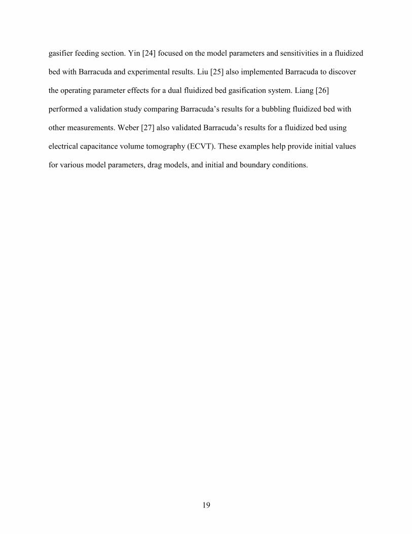
Figure 3-3: Two plots from each case showing the variation of the mass flow rate of the coal with respect to time (first column) and a histogram of the probability density of the coal mass flow rate with respect to coal mass flow rate over entire time period through a flux plane at the end of the system (second column). Top row: Case M1. Middle row: Case M2. Bottom row: Case M3. .......................................................................................................... 30

Figure 3-4: Particle volume fraction screen-shot and cross section view of Case M1 after running for 10 seconds. ....................................................................................................................... 31

Figure 3-5: Particle and gas velocity profiles at the exit of the system for Case M1. .................. 31

Figure 3-6: Comparison of the initial test case (left) and the updated test case (right) to simulate a more realistic starting condition. The remaining vertical and horizontal sections are cut off in these schematics. ............................................................................................................... 33

Figure 3-7. a) Mass flow rate of coal versus time. b) A histogram plot on the probability density versus the mass flow rate of coal. .......................................................................................... 34

Figure 3-8: Coal mass flow rate exiting the pipe versus time....................................................... 40

Figure 3-9: All plots are exiting coal mass flow rate with respect to time. Top-left: averaging every 10 points. Top-right: averaging every 100 points. Bottom-left: averaging every 1000 points. Bottom-right: averaging every 10000 points. ............................................................ 41

Figure 4-1: Plots of coal mass remaining in the system versus time. ........................................... 49

viii

Figure 4-2: Geometry of the angled hopper with the same amount of mass and same boundary and initial conditions as the original gravity-fed system discussed in Section 4.1. .............. 50

Figure 4-3: The initial gravity-fed geometry is shown in the top image and the particles are shown mid-simulation. The modified geometry with the angled conical hopper is shown in the bottom image with the particles also shown mid-simulation. The operating pressure was 2.0 MPa and the CO2 mass flow rate was 0.004 kg/s ............................................................ 52

Figure 5-1: CAD geometry of the fluidized bed system. .............................................................. 55

Figure 5-2: Non-uniform mesh of the fluidized bed with a uniform inlet. Smaller cells were implemented in the 0.635-cm diameter pipe with larger cells in the 5.08-cm diameter hopper. ................................................................................................................................... 56

Figure 5-3: Two geometries used to test fluidization: Uniform inlet (left, Case F1) and concentrated central inlet (right, Case F2). ........................................................................... 57

Figure 5-4: Inside look (geometry cut in half) at the particle volume fraction in the first geometry looking at fluidization and the particle characteristics every second from zero to seven seconds. ................................................................................................................................. 58

Figure 5-5: Same case as Figure 5-3, but with a bigger pressure boundary condition for the outlet of CO2 at the top of the hopper. ............................................................................................. 60

Figure 5-6: Look inside of the particle volume fraction for the second geometry, Case F2, (0.635-cm diameter inlet) every second from zero to seven seconds. .............................................. 61

Figure 5-7: Modified geometry of the fluidized bed to test exiting coal mass flow rates and CO2-to-coal mass ratios. The uniform inlet (left) and concentrated central inlet (right) are shown. ............................................................................................................................................... 63

Figure 5-8: Geometries for the: a) 15-cm diameter hopper and b) the transitional 5-to-15-cm diameter hopper. .................................................................................................................... 66

Figure 5-9: Central cross-section of Case F13 (Uniform, left), Case F14 (1 Jet, middle), and Case F15 (5 Jets, right) and their respective particle volume fractions after 30 seconds of simulation. The inlet boundary condition is shown to the left of each respective geometry. 69

Figure 6-1: Geometry of the 60.96-cm long system. .................................................................... 72

Figure 6-2: Case P1 snapshot of the 60.96-cm long pipe mid-simulation. The bottom zoomed out image depicts the layout of particles as the flow continues towards the exit. The top zoomed- in portion portrays the last 10-cm of the pipe and formation of two dunes. .......... 73

Figure 6-3: Snapshot of the 121.92-cm long system mid-simulation. The right hand side of the pipes is the end of the system. The left side of the pipes continue on to the rest of the system. The bottom pipe represents about the last 10-cm with the top pipe representing the last 40-cm of the system. ....................................................................................................... 75

ix

Figure 6-4: Original data for the mass flow rates of coal (black) and CO2 (light gray) versus time at the exit of the system for the 60.96-cm long pipe (left) and the 121.92-cm long pipe (right). .................................................................................................................................... 76

Figure 6-5: Averaged-down data shown to compare with the data recorded in Figure 6-4) The 60.96-cm horizontal pipe test is on the left and the 121.92-cm horizontal pipe is on the right. ............................................................................................................................................... 77

Figure 6-6: Comparing the 121.91-cm long pipe for two different CO2 mass flow rates causing 1-to-1 and 2-to-1 gas loading ratios. ......................................................................................... 79

Figure 6-7: Particle size distribution for the coal used in most simulations. ................................ 80

Figure 6-8: View of the particle radius looking down the end of pipe (last 7.62 cm) with the flow coming out of the page. Top, side, and bottom views are also shown with the flow direction indicated with arrows. ........................................................................................................... 80

Figure 6-9: Schematic showing orientation of the three sharp 90° bends (left) and the three larger bend radii (right) mapped on a Cartesian coordinate system. ............................................... 82

Figure 6-10: Particle flow showing roping around a 90° downward bend in a 0.635-cm diameter pipe. Particles are flowing from the left to the right and downward. .................................... 83

Figure 6-11: Particles of Case HH1 mid-simulation with the front view particles flowing from left to right (top) and back view particles flowing from right to left (bottom) shown of the horizontal 90° bend. .............................................................................................................. 86

Figure 6-12: Snapshot of the particles at the end of the bend after ten seconds of simulation of Case HH3 (left) and Case HH4 (right). Left of each gray circle is where the bend ends. This view is looking straight into the exit of the pipe with particles and gas coming out of the page........................................................................................................................................ 87

Figure 6-13: Particles in the entire pipe shown for Case HU5 as well as the cross-section at beginning of the pipe (bottom left) and at the end of the pipe (top right). ............................ 90

Figure 6-14: Particle volume fraction comparison of each of the horizontal-to-upward vertical tests looking down at the exit and into the pipe 7.62 cm. ..................................................... 91

Figure 6-15: Particle volume fraction of the entire pipe shown for Case HD9. The inlet (left) and outlet (right) cross-section are also shown to observe the roping effects of at the outlet. Gravity is in the negative Z-direction. ................................................................................... 93

Figure 6-16: Particle volume fraction comparison of each of the horizontal-to-downward vertical tests looking up at the exit and into the pipe 7.62 cm. .......................................................... 94

Figure 6-17: A side view of the particle volume fraction for Cases HD11-HD14. Cases HD11 and HD12 are the 60.96-cm bend radius and Cases HD13 and HD14 are the 182.88-cm bend radius. .................................................................................................................................... 95

x

Figure 6-18: Cross-section view of the mesh for each pipe exit. Each color represents the area where a flux plane was placed to record results. ................................................................... 96

Figure 6-19: Coal mass flow rate plotted versus the vertical area section in the pipe for the horizontal-to-horizontal bend tests (Cases HH1-4). ............................................................ 100

Figure 6-20: Coal mass flow rate plotted versus the vertical area section in the pipe for the horizontal-to-upward vertical bend tests (Cases HU5-8). ................................................... 101

Figure 6-21: Coal mass flow rate plotted versus the vertical area section in the pipe for the horizontal-to-downward vertical bend tests (Cases HD9-14). ............................................ 102

Figure 6-22: Schematic for new geometry looking at roping effects with changing pressure. .. 104

Figure 6-23: Coal mass flow rate plotted versus the vertical area section in the pipe for extended horizontal-to-downward vertical bend with varying pressures. .......................................... 106

Figure 6-24: Geometry of the two-bend system with the flow directions indicated. ................. 108

1

1 INTRODUCTION

Coal combustion has been widely used since the 1800s to generate power. Even with the

dawning of inexpensive natural gas, coal continues to be a major source of electricity in the

United States [1]. One of the challenges with coal combustion is the greenhouse gases created

and released into the environment, primarily carbon dioxide (CO2) [2]. A potential approach to

reduce CO2 emissions involves the use of oxy-coal combustion, where coal is burned with pure

oxygen, rather than air as is commonly done [3]. This process creates a higher purity CO2 flue

gas stream which is readily captured for recirculation, storage, or industrial use. A challenge with

oxy-coal combustion is decreased plant efficiency due to parasitic power losses associated with

the production of oxygen. Inefficiencies associated with oxygen firing may be partially offset by

the use of pressurized oxy-coal (POC) combustion. Combustion of oxygen and coal at high

pressures can provide higher efficiency power cycles due to enhanced thermal energy recovery

[3] [4].

Current industrial coal combustors and feed systems usually operate at atmospheric

pressure. At this pressure the coal is fed into the reactor typically with a screw-feeder or a

gravity-fed system. At high pressures, a slurry method which mixes coal and water is utilized to

feed coal into a combustor. This approach is efficient in transporting the coal, but energy is lost

in the combustor because of the water that needs to be heated up and evaporated during the

combustion process [5] [6]. A pressurized oxy-coal combustor with a pressurized dry feed

2

system will maximize combustion and cycle efficiency. This system uses pressurized CO2 to

transport coal to the combustor and feed it into the pressurized combustor. Such a system has not

been designed and tested in industry. This project seeks to guide the design of a pressurized dry

coal-feed system for a pilot-scale POC reactor using computational fluid dynamics simulations.

A POC reactor is being constructed at Brigham Young University with funding from the

U.S. Department of Energy (DOE) to study design and performance issues related to pressurized

oxy-coal combustion, including a dry coal-feed system. This reactor is designed to operate at

2.07 MPa (20.4 atm or 300 psi), with a 100 kWt firing rate. Based on bituminous coal with a

higher heating value of 26.5 kJ/kg the coal mass flow rate should be 0.00378 kg/s and the gas-to-

coal mass flow ratio should be anywhere from 1 to 2. Coal particles are conveyed to the reactor

with carbon dioxide (CO2) and combusted with oxygen (O2). The first step of the reactor process,

a feed system, is required to produce a steady and uniformly dispersed flow of coal into the

reactor at pressure. To produce a steady and uniformly dispersed flow, coal particles in a

pressurized pipe must be pneumatically transported from a stationary packed bed and into the

reactor.

1.1 Feed System Components

This section outlines key components of the pressurized coal-feed system. The feed

system needs to deliver coal particles and gas (CO2) to the reactor from a pressurized hopper of

stationary particles. As shown in Figure 1-1, the reactor is downward firing and the coal and CO2

enter from the top of the reactor and create a downward flame. The feed piping should transport

a sufficient amount of coal from the hopper to the reactor. Coal flow sufficient to produce a 100

kWt flame was required. The hopper size and shape were flexible, but needed to allow pilot-scale

3

operation for at least eight hours. Since the hopper will be located in a fuel room adjacent to the

reactor, the piping system will include multiple 90-degree bends and horizontal and vertical runs.

1.2 Objective

The objective of this research is to develop and use a computational model to design a

conceptual, pilot-scale pressurized coal-feed system. Both a steady and uniformly dispersed flow

were desired in the coal-feed coming into the reactor. A steady flow is a flow that does not

change with time. It is important for a feed system to deliver a steady amount of fuel and gas to a

reactor to ensure complete combustion and constant flame length. A uniform or uniformly

Figure 1-1: Schematic of the feed system including the hopper, piping system, and reactor.

g

4

dispersed flow is a flow that fills up the entirety of the feed pipe cross-section. The flow should

be homogenous meaning the flow is uniform within the pipe. If the flow is not uniform and there

is a build-up of coal on a particular side of the inlet, this can affect flame length and stability and

contribute to incomplete mixing of the coal particles with the oxidant (O2).

The research objective was accomplished by completing the following tasks:

• Identify the appropriate Barracuda software model settings to represent flow

behavior in the pressurized dense particle system,

• Evaluate the ability of two different feed system designs to deliver steady coal

flow from a vertical packed coal bed to a pilot-scale POC reactor at desired carrier

gas and coal mass flow rates,

• Quantify the coal particle distribution and pressure drop for different piping system

components,

• Recommend conceptual feed system design and summarize key design principles

that can be applied to future pressurized dry-feed systems.

The flow rate exiting a piping section was considered steady if the standard deviation of

the coal flow rate was less than or equal to 5%, or 0.05 of the average coal mass flow rate. For

flame and burner stability, this value was chosen to provide an adequately steady flow of coal

into the reactor. The mass flow rate of coal can fluctuate coming into the reactor, but it should be

steady enough to allow continuous coal combustion. Based on conversations with the research

group designing the burner, the burner can allow fluctuations on the order of one second. Thus

the metric for steady flow was a ratio of standard deviation to average coal mass flow rate less

than 0.05 at a time average of one second.

5

While steadiness was the primary performance metric, coal flow uniformity exiting a

piping section was also measured. The flow was uniformly dispersed if there was 50% of the

mass flow rate on both halves of the pipe, or a 50-50 dispersed flow. The acceptable limit for

uniformity was 60-40, where there was 60% of the flow on one-half of the pipe and the

remaining 40% of the flow was on the other half. If more than 60% of the coal was in one-half of

the pipe at the burner, there was increased potential for a non-uniform flame in the reactor.

Depending on the direction of the flow, the two halves of the pipe to measure uniformity could

be the top and bottom, or left and right. The uniformity metric is not as significant as the

steadiness metric because the coal dispersion will vary through the piping system before

reaching the burner and the coal inlet area at the burner is 32 times smaller than the combustor

cross-sectional area, so biases in the coal inlet will be small relative to the flame location in the

reactor.

6

2 BACKGROUND

The feed system involves two main flow processes: vertically oriented fluidization and

horizontal pneumatic transport. Vertical fluidization is important in the beginning of the feed

system to allow the particles inside of the hopper to fluidize and exit the hopper. Fluidization

helps the coal particles flow as if it were a fluid causing the particle and gas mixture to more

easily exit the hopper into the piping system. Once the particles are in the piping system, they are

transported to the reactor using horizontal as well as vertical transport.

When the hopper, or bed of particles, is fluidized a steady flow rate of coal is expected to

exit the hopper. This coal mass flow rate can be adjusted using the mass flow controllers for the

amount of CO2 that is used to fluidize the hopper. The ratio of CO2-to-coal required for

fluidization is likely smaller than the desired ratio entering the reactor. This is desirable as it

allows additional CO2 to be added to the carrier gas to dilute the flow and enhance horizontal

transport while acquiring a desirable gas-to-particle flow rate ratio prior to entering the reactor.

The design key is to start on the low end of CO2-to-coal ratio and ensure that the entire hopper

(coal bed) is fluidized yielding a coal mass flow rate greater than or equal to the CO2 mass flow

rate exiting the hopper. Additional CO2 can then be added post-hopper exit to control pneumatic

transport to the POC.

7

1.2. Fluidization

Fluidization of a bed of particles depends on several factors, including particle properties,

gas properties, and feed system geometry. Fluidization is utilized in industry with circulating

fluidized beds (CFBs) for coal gasification, combustion, fluid catalytic cracking (FCC), and

chemical looping. Many current applications are in vertical chambers or risers. Fluidization is

defined as the operation through which granular solids, or a bed of particles, is transformed into a

fluid-like state through contact with either a gas or a liquid [7]. The fluid being pumped into the

bed needs to have a high enough velocity/flow rate to overcome the particles’ weight with an

upward drag force as shown in Figure 2-1.

The fluid velocity required to initiate fluidization is termed the ‘minimum fluidization

velocity.’ It is a function of the densities of the fluid and particles, gravity, particle diameter,

viscosity of the fluid, and the bed void fraction. As the gas velocity is increased beyond the

minimum fluidization velocity, the particles in the bed are pneumatically transported. This

Figure 2-1: Forces on a single particle in a fluidized bed.

8

increased velocity minimizes the potential for clogging of particles. Clogging is where particles

stick together usually due to moisture content of the particles. If clogging occurs the coal mass

flow rate will stop indefinitely. Of the six stages depicted in Figure 2-2, anywhere from a

fluidized bed (Stage 3) to a fluidized bed in good condition (Stage 4) is desired in the feed

system to ensure a constant movement of coal particles. Although Stage 2 is the minimum

fluidization state and should be able to transport enough coal, to be sure that clogging, bridging,

or ratholing do not occur in the system, Stage 3, or the minimum bubbling state is the target.

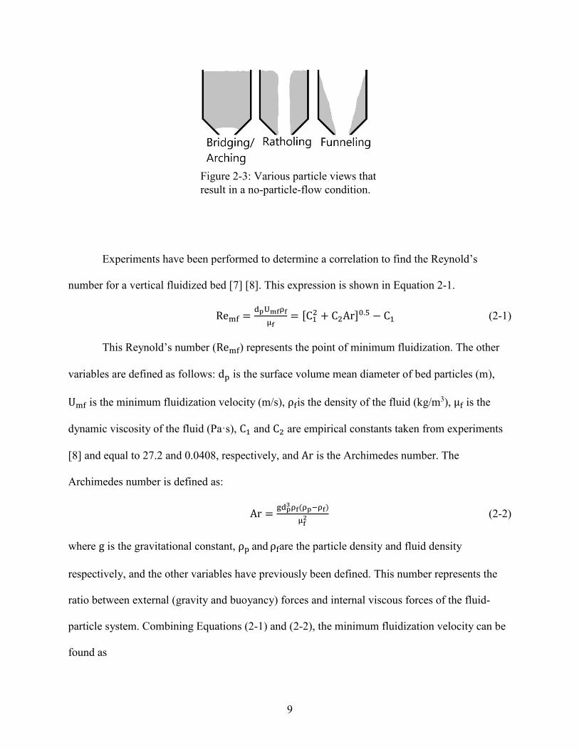
Figure 2-3 exhibits bridging, ratholing, and funneling. Bridging, or arching is similar to clogging

and causes a bridge, or arch from one wall of the hopper to the other and no particles drop from

that blockade. Ratholing is where a hole is formed in the middle of the hopper keeping the

surrounding particles in place. A less severe form of ratholing is funneling where particles are

still left on the sides and they form a funnel from the top of the hopper down to the bottom. All

of these conditions can lead to the undesirable occurance of a large quantity of coal suddenly

dropping into a feed system.

Figure 2-2: Stages of fluidization in a vertical riser [35].

9

Experiments have been performed to determine a correlation to find the Reynold’s

number for a vertical fluidized bed [7] [8]. This expression is shown in Equation 2-1.

Remf = dpUmfρfμf

= [C12 + C2Ar]0.5 − C1 (2-1)

This Reynold’s number (Remf) represents the point of minimum fluidization. The other

variables are defined as follows: dp is the surface volume mean diameter of bed particles (m),

Umf is the minimum fluidization velocity (m/s), ρfis the density of the fluid (kg/m3), μf is the

dynamic viscosity of the fluid (Pa·s), C1 and C2 are empirical constants taken from experiments

[8] and equal to 27.2 and 0.0408, respectively, and Ar is the Archimedes number. The

Archimedes number is defined as:

Ar = gdp3ρf(ρp−ρf)μf2 (2-2)

where g is the gravitational constant, ρp and ρfare the particle density and fluid density

respectively, and the other variables have previously been defined. This number represents the

ratio between external (gravity and buoyancy) forces and internal viscous forces of the fluid-

particle system. Combining Equations (2-1) and (2-2), the minimum fluidization velocity can be

found as

Figure 2-3: Various particle views that result in a no-particle-flow condition.

10

Umf = μfρfdp

�C12 + C2 �gdp3ρf�ρp−ρf�

μf2 ��

0.5− C1 (2-3)

Once the minimum fluidization velocity is solved for in Equation 2-1, the bubbling

velocity (Umb) can be solved for in the equation given by Abrahamsen and Geldart [9]:

UmbUmf

= 2300μf0.523ρg0.126e(0.716F)

dp0.8g0.934�ρp−ρg�0.934 (2-4)

All the variables have previously been defined except for F which is the mass fraction of

particles less than 45 μm, g is the acceleration due to gravity (m/s2), and ρp is the density of a

bed particle (kg/m3). The bubbling velocity represents the point at which bubbles of gas will start

to form in the bed and move upwards. This velocity is larger than the minimum fluidization

velocity.

In fluidization research, silica particles are typically used because they are spherical, or

have a sphericity approximately equal to one. Sphericity is a measure of how spherical an object

is and is defined as the ratio of the surface area of a sphere (with the same volume as the given

particle) to the surface area of the particle. Compared with silica, coal is non-spherical and

requires a greater velocity to be pneumatically transported. The random bumps and edges of non-

spherical particles cause a randomness in the flow and can lead to difficulty in developing

relations and predictions of the flow. For non-spherical particles, there is a significant increase in

the contact points between particles-to-particles and particles-to-wall and this leads to an

increase in cohesive forces and thus a greater velocity is needed to fluidize and transport the

particles [10].

Shabanian and Chaouki [11] focused on how temperature, pressure, and inter-particle

forces affect the hydrodynamics of gas-solid fluidized beds. They found that increasing pressure

reduces the minimum fluidization velocity for particles larger than 200 µm. At this size, inertial

11

effects begin to dominate and with larger sized-particles the effect is more pronounced.

Approximately 10-15% of the coal particles are expected to exceed 200 µm and high pressures

may lead to lower gas flow rates needed to fluidize and transport the particles. As pressure

increases, for a constant mass flow rate (m), the density (ρ) increases and the velocity (v)

decreases assuming the same cross-sectional area (A) as shown in Equation 2-5.

m = ρfvA (2-5)

2.1 Horizontal Pneumatic Transport

Horizontal pneumatic transport is a step past fluidization. It is the moment when particles

start to physically be picked up and moved along a pipe. Horizontal particle flow requires a

greater gas velocity compared to a vertical flow to maintain uniformity of the coal particle

distribution across the pipe because of layout in the pipe. One of the characteristics of horizontal

two-phase flow (gas and solid) is that larger particles tend to group on the bottom of the pipe

whereas the smaller particles tend to stay uniformly dispersed in the pipe and flow more easily

[12].

The Reynolds number is a non-dimensional number typically used for categorizing the

pipe flow as laminar or turbulent. For dual-phase flow, the Reynolds number, Re , is defined as:

Re = ρfvdpμf

(2-6)

where ρf is the fluid density, v is the velocity of the fluid, sometimes referred to as the superficial

velocity, dp is the particle diameter, and μf is the fluid viscosity. Researchers have developed

relationships between the Archimedes and Reynolds numbers with slight modifications to the

latter to define three zones which describe the superficial velocity in a particle-fluid system and

12

the corresponding type of flow [13]. The Archimedes number and modified Reynolds number

relations for the three zones are shown in Figure 2-4.

The three zones deal with varying pickup velocity, particle diameter, and inter-particle

cohesive forces. The three zones are: Zone 1) where the particle pickup velocity increases as the

particle diameter increases due to an increase of the gravity force; Zone 2) where the pickup

velocity increases as the particle diameter decreases due to an increase in cohesive forces; and

Zone 3) where powders (small particles) are so cohesive that the particles move as agglomerates

rather than single particles [13] [14]. The modified Reynolds number plotted in Figure 2-4, Rep∗ ,

is defined as:

Rep∗ = ρfUpud

μ�1.4−0.8∙exp�−DD501.5 ��

(2-7)

The variables include ρf for fluid density, Upu is the pickup velocity (gas velocity when pickup

from a layer of particles begins), d is the particle diameter, μ is the gas dynamic viscosity, D is

the pipe inside diameter or wind tunnel height, D50 is the pipe inside diameter of the experiment,

or 50-mm [13]. This experiment was run specifically to find the pickup, or critical velocity of

particles in a 50-mm diameter pipe. Of the multiple correlations that exist in the literature, this is

the correlation that seemed to best correspond to the geometry and conditions in the pilot-scale

feed system. Cabrejos and Klinzing [15] have used experimental data to predict the minimum

pickup velocity based on a model for the initial motion of a single particle, the boundary layer

thickness, and the Archimedes number.

Kalman et al. [23] established the relations in Figure 2-4 by combining others data and

their own and found 90% of the measured points were within the limits of ±30% of the

correlations [13] [16]. The three relations as seen on Figure 2-4 are valid over a wide range of

13

particle properties, including when: 0.5<Rep*<5400, 2 x 10-5<Ar<8.7 x 107, 0.53<d<3675 μm,

1119<ρp<8785 kg/m3, and 1.18<ρ<2.04 kg/m3. The problem with these relations is that they do

not apply at high pressures. A relation was sought for higher pressures, but most relations apply

at atmospheric pressure (0.101 MPa). Knowing the relationships were meant for lower pressures,

the graph in Figure 2-4 and previously defined equations were used in the research as an estimate

of the Reynolds number and a pickup velocity was calculated. This number was used to guide

the flow rates tested to see if similar behavior ensued.

A visual overview of dual-phase horizontal flow is shown in Figure 2-5, which plots flow

regimes as a function of particle Froude number and the particle Reynolds number. Both Froude

Figure 2-4: Three zones model identifying particle pickup and non-pickup regimes as a function of modified Reynolds number and Archimedes number [14].

14

and Reynolds numbers here are based on the particle diameter. The Froude number is a ratio of

inertial and gravitational forces while the Reynolds number is a ratio of inertial to viscous forces.

The regime sought after is the ‘homogenous gas-solids flow.’ This type of flow would provide

both a uniform and steady flow of gas and solids to the reactor.

If the velocity of the fluid is too low, then the flow encounters an undesired type of flow

as shown in Figure 2-5, including: stratified flow, pulsating flow, moving dune-flow, saltation

flow, flow over a settled layer, and minimal pickup flow. The saltation point, or saltation

velocity for horizontal pneumatic conveyance is the minimum velocity of the fluid needed to

transport all the particles. The gas velocity needs to be greater than the saltation velocity to

Figure 2-5: Model of flow regimes observed for horizontal pneumatic conveying including pickup and saltation regimes with the Froude versus Reynolds numbers [16].

15

achieve a steady and uniform flow of gas and solids. Otherwise, the particles start to layout along

the bottom of the pipe. To achieve minimal layout, the pickup velocity was calculated. Various

correlations exist for the pickup velocity and it was helpful to find these equations gave pickup

velocities that were on the same order of magnitude [13] [17]. The pickup velocity equations are

as follows. For a single small particle on a flat plate in shear flow, Hayden et al. [18] found that:

Upu = 2.62ν�1321�D�

321�

μ821

�π6

g�ρp − ρg� + 1.302∙10−6

d2�821. (2-8)

As a preliminary result matching their experiments, Kalman et al. [13] found that:

Upu = 2.66μAr0.474

ρgd. (2-9)

Kalman’s experiments consisted of a rectangular wind tunnel that had a cross section of 0.1 x 0.1

m. Air was used as the conveying gas and various particles were used such as glass, zirconium,

alumina, iron, and salt. Combining their findings with other results published in the literature,

Kalman et al. adjusted their equation to be:

Upu =Rep

∗ μ�1.4−0.8∙exp�−DD501.5 ��

ρfd , (2-10)

which is a different form of Equation (2-7). These equations provided ranges of what the

horizontal velocity needed to be to pick up and transport the coal particles in the feed system.

The path from the coal hopper to the reactor requires different bends, or turns in the

piping system. The coal and CO2 travels horizontally or vertically and depending on the bend

direction and radius, the dual-phase flow behaves differently. When particle laden flow travels

around any type of bend, or turn in a pipe, roping often occurs. Roping is the physical

phenomena of particles coalescing on the far side of the bend. A number of researchers have

16

published information on the layout of particles and the effect of bend radius on flow, roping and

downstream behavior [19] [20] [21]. This is covered in greater detail in Chapter 6.

2.2 Barracuda CFD Software

Barracuda Virtual Reactor 17 is a software package from CPFD Software (Computational

Particle Fluid Dynamics) that specializes in modeling gas-solid flows, particularly dense phase

flows [22]. Barracuda was utilized in the running of all simulations. Commercial computational

fluid dynamics (CFD) software such as Fluent, Star-CCM+, and OpenFOAM typically look at

one fluid flow or multiple fluids with reactions in, over, and around various objects. Barracuda

incorporates particles into their fluid flow and tracks the fluid as well as the particles in a

particular geometry. This software is useful for testing different scenarios and systems without

building multiple hardware configurations to run experiments. Simulations are useful for

screening different design concepts and narrowing design and operating possibilities. This

information can then be used to guide the design of prototype experiments as well as the final

system design and operating conditions.

A geometry is created in a CAD (Computer Aided Design) software and is imported into

Barracuda as an STL (stereolithography) file. A mesh, or grid, is created to fit the geometry and

must be fine enough to capture the physics but relatively coarse to have a reasonable run time. A

two-dimensional mesh is shown in Figure 2-6. Specific to Barracuda, the mesh is a structured

grid which implies that all the cells created are square or rectangular. A mesh is needed in the

code to breakdown a large geometry into a finite number of cells, and solve the flow equations

for each cell. Barracuda incorporates an Eulerian-Lagrangian approach for simulating particle-

fluid flow. The particles are modeled as discrete Lagrangian points and the fluid is modeled on

an Eulerian grid of cells. After the mesh is generated, global settings like gravity and temperature

17

are defined. The initial conditions (fluids and particles) and boundary conditions (fluid flow,

particle flow, pressure) are defined and the case is ready to run.

Sub-model parameters are defined according to the type of flow and media flowing.

These parameters include the close pack volume fraction, the maximum momentum redirection

from particle-to-particle collisions, and the normal-to-wall momentum retention and tangent-to-

wall momentum retention for the particle-to-wall interactions. Particles and fluids are imported

from libraries or created and defined. A drag model (e.g., Constant, Stokes, Wen-Yu, Ergun,

WenYu-Ergun, Turton-Levenspiel, etc.) [22] is selected based on the type of particles and type

of flow. Depending on the size of the geometry and mesh, runtimes for cases can last anywhere

from a couple of hours to a couple of days.

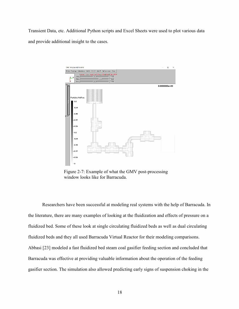
After cases were run to completion, the results were studied looking at the mass flow of

particles and gas, gas velocity, particle volume fraction, gas density, drag, etc. using the

Barracuda post-processing tool called GMV, or General Mesh Viewer. An example of what the

GMV window looks like is shown in Figure 2-7. This tool helped visualize the geometry and the

flow of the system. Other data outputs were used including Flux Planes, Averages, 2D Plots,

Figure 2-6: Various mesh sizes for a circular pipe ranging from coarse (left) to fine (right).

18

Transient Data, etc. Additional Python scripts and Excel Sheets were used to plot various data

and provide additional insight to the cases.

Researchers have been successful at modeling real systems with the help of Barracuda. In

the literature, there are many examples of looking at the fluidization and effects of pressure on a

fluidized bed. Some of these look at single circulating fluidized beds as well as dual circulating

fluidized beds and they all used Barracuda Virtual Reactor for their modeling comparisons.

Abbasi [23] modeled a fast fluidized bed steam coal gasifier feeding section and concluded that

Barracuda was effective at providing valuable information about the operation of the feeding

gasifier section. The simulation also allowed predicting early signs of suspension choking in the

Figure 2-7: Example of what the GMV post-processing window looks like for Barracuda.

19

gasifier feeding section. Yin [24] focused on the model parameters and sensitivities in a fluidized

bed with Barracuda and experimental results. Liu [25] also implemented Barracuda to discover

the operating parameter effects for a dual fluidized bed gasification system. Liang [26]

performed a validation study comparing Barracuda’s results for a bubbling fluidized bed with

other measurements. Weber [27] also validated Barracuda’s results for a fluidized bed using

electrical capacitance volume tomography (ECVT). These examples help provide initial values

for various model parameters, drag models, and initial and boundary conditions.

20

3 MODEL DEVELOPMENT

A computational fluid dynamics (CFD) model of the coal-feed system is needed to

evaluate the performance of different system designs and operating conditions that would be

difficult or expensive to test experimentally. To develop confidence in such a model, it is useful

to assess the impacts of different model parameters such as mesh sensitivity and particle sub-

models. The development of a baseline model also helps identify which model outputs are most

valuable in assessing predicted results. This chapter describes the development of a gravity-fed

model which was assumed would be an effective design to transport the coal. Within the gravity-

fed model, mesh sensitivity and sub-model parameter sensitivity studies were performed and

methods for assessing transport performance were identified.

The key assumptions in modeling the feed system were as follows.

• All hopper and piping walls were assumed to be smooth. Particle-wall interactions

assumed smooth walls and there was no pressure drop due to rough surfaces.

• All particles were assumed to be spherical (see discussion in Section 3.2).

• There was no particle attrition in the model. Initial particle size and particle size

distribution in the hopper remained constant throughout the simulation. In reality,

small pieces of non-spherical coal particles will break off as the particles collide

with each other and the walls.

• Coal particles had zero moisture content. Bridging and cohesion effects due to

moisture were not modeled.

21

• The CO2 gas was treated as an ideal gas at all pressures. The gas and particle flow

was isothermal and non-reactive. Any energy dissipated between particle-wall or

particle-particle interactions did not change the gas or particle temperature.

• Simulations were run until the coal hopper was empty or for about 20 to 30

seconds. It was assumed that when the coal mass flow rate leveled out and was

unchanging, the flow was steady state. At this point, flow rates, steadiness, and

particle dispersion were assumed to continue indefinitely based on the values at

the end of the simulation.

• A time-averaged rate of one second was used to quantify the steadiness of the

flow (see discussion in Section 3.5).

3.1 Initial Geometry

The geometry of the first model investigated consists of an L-shaped pipe as seen in

Figure 3-1 and hereafter will be referred to as the gravity-fed system. The initial vertical section

was 12.7 centimeters (cm) in height. The vertical standpipe connected with a longer horizontal

section. The horizontal section, to the right of the standpipe was 30.5 cm long and to the left was

0.76 cm long. The CO2 entered from the left side of the horizontal section and exited out the

right side. The interior diameter of all pipes was 0.635 cm. In this gravity-fed system, the coal

was initially positioned in the vertical standpipe and allowed to drop into the horizontal flow of

CO2. The purpose for this design was to let gravity do the work and only have need of one CO2

inlet to transport the dropping coal.

22

3.2 Barracuda Model Parameters

Barracuda creates a computational mesh based on a distribution of three-dimensional

uniform square cells or prisms. The spacing and sizing of the mesh can be changed, but it

remains rectangular prisms. Because a cylindrical geometry is being broken up into cubes, it was

important to have enough cells to accurately represent the round duct shape. Barracuda creates

both real and null cells around the geometry, and this creates a 30.5 cm x 12.7 cm x 0.635 cm

rectangular “box” to encapsulate the entire feed system. Cells within the pipe flow are

considered real cells. Those outside the pipe are null cells. Calculations are performed only in

real cells, not in null cells.

The simulations were run at a constant temperature of 300 K with a bituminous

Pittsburgh coal and carbon dioxide (CO2). Each coal particle had a diameter of 75 µm and a

density of 1300 kg/m3, and was assumed spherical (sphericity, or ψ = 1). The carbon dioxide

Figure 3-1: Schematic of the gravity-fed system (all dimensions are in cm).

23

(CO2), which had a density of 1.782 kg/m3 at 0.101 MPa, had a density 35.29 kg/m3 at 2 MPa.

Regarding the particle-to-particle interaction, the close pack volume fraction was equal to 0.6

and the initial packing fraction was equal to 0.4. The maximum momentum redirection from

collision was 40%. For particle-to-wall interaction, the normal-to-wall momentum retention as

well as the tangent-to-wall momentum retention was 0.8 with a diffuse bounce of zero. Friction

and restitution values will affect particle velocity, solid concentration (particle volume fraction),

and pressure drop considerably [28] [29].

The particle drag model was important as it defines the main interaction between gas and

particles. There are many choices for a drag model in Barracuda. The Wen-Yu-Ergun drag model

was selected as the most fitting for this research based on its accuracy in prediction of gas-

particle behavior for the particle diameters and flow conditions studied here. Its performance has

been documented in previous experiments and simulations in the literature [23] [26] [30] [31].

The Wen-Yu model is appropriate for dilute-phase flow and the Ergun model is appropriate for

dense-phase flow. This combined drag model assumes a particle sphericity equal to one.

While sphericity can play an important role in particle behavior, it was not a major focus

in this study. A few simulations were run with only changing the sphericity and are discussed in

Chapter 4.Gomes [10], Chhabra [32], and Militzer [33] have each performed in depth studies of

sphericity and the effect it has on drag and the pickup velocity of particles. They found that as

the sphericity decreased, or as the particles were less spherical (ψ < 1), the pickup velocity

increased. For Reynolds numbers less than 100, non-spherical particles had a higher coefficient

of drag and thus, more drag than spherical particles. The Reynolds number for one-to-one coal-

to-gas flow (both at 0.00378 kg/s) at 2 MPa would be equal to 0.376 which corresponds to a

laminar flow. Because the flow is laminar, the velocities taken from the simulations should be

24

expected to be higher than the actual velocity from the real system. This is because of sphericity.

A coal particle is not a perfect sphere, but has lots of rough edges and sharp points. These edges

and point will catch with the pipe wall and other particles and will not move in the same way as

spherical particles do. This will lead to added momentum losses and a slower particle velocity.

To compensate for the sphericity of particles in actual experiments and to achieve the same

particle flow behavior as seen in these cases, additional flow will be needed than predicted.

3.3 Mesh Sensitivity

A mesh sensitivity test was performed to determine how fine of a mesh was needed for

the interior of the pipe. The mesh refinement impacts the following aspects of the computations:

the starting mass of coal particles, the coal mass flow rate exiting the system, and the pressure

drop in the system. This study was important because the results of the simulation may change

depending on the mesh. The mesh chosen was ascertained based on comparing the results with

other meshes that were coarser or finer.

Three different meshes were tested to observe the differences in coal flow steadiness. In

each case, all other model parameters were kept the same except for the number of mesh cells.

Figure 3-2 shows the computational meshes at the junction of the standpipe and horizontal duct

for each of the three cases. For Case M1, each interior cell size was equal to 0.50 mm and across

the diameter of the pipe there were 13 cells; vertically there were 257 cells and horizontally there

were 618 cells. For Case M2, each interior cell was equal to 0.40 mm and across the diameter of

the pipe there were 16 cells; vertically there were 324 cells and horizontally there were 778 cells.

For Case M3, each interior cell was equal to 0.32 mm and across the diameter of the pipe there

were 20 cells; vertically there were 408 cells and horizontally there were 981 cells. These cases

25

are referred to with an ‘M’ signifying a case in the model development chapter. The cell size is

important to know because it defines the limits of how many particles are able to fit inside one

cell. The cell size does not have to be significantly larger than the largest particle size, but it

should allow for four to five particles across the cell. Case M3 has the smallest cell size and

pushes the limit of the cell size to particle size ratio. Dividing the 0.32 mm cell size by the 0.075

mm particle diameter, this results in 4.3 particles per cell.

The pressure was kept at 2 MPa for Cases M1, M2, and M3. Case M1 was considered the

base case. Case M2 kept the same volume of the pipe occupied by particles, but the mesh was

refined to double the amount of Case M1 cells. Case M3 quadrupled the amount of cells in the

base case (Case M1). Case M2 and Case M3 increased the number of cells in all directions (x, y,

and z). To double or quadruple the number of cells, the cell size decreased from 0.50mm (Case

M1) to 0.40mm (Case M2) to 0.32mm (Case M3). Each mesh incorporated a uniform spacing

and an equal size of cells. Table 3-1 summarizes each of the three cases. From left to right, the

columns record the case number, the total number of cells, the number of real cells, the number

of null cells, the number of particles, the total mass of coal particles starting in the system, the

average CO2 mass flow rate exiting the system, the average coal mass flow rate exiting the

a) b)

Figure 3-2: Snapshots of the meshing for each case: a) Case M1, b) Case M2, c) Case M3.

c)

26

system, and the pressure drop calculated from the beginning of the vertical standpipe to the exit

of the system.

Table 3-1: Simulation Values for Varying Mesh Sizes

Case Total

Number of Cells

Real Cells

Null Cells

Particle Count

Total Mass (kg)

Avg. CO2 Mass Flow Rate (kg/s)

Avg. Coal Mass Flow Rate (kg/s)

Pressure Drop (Pa)

M1 1.91E+6 120,000 1.79E+6 7.49E+06 2.15 E-3 4.0 E-3 3.60 E-3 535 M2 3.78E+6 220,000 3.56E+6 7.63E+06 2.19 E-3 4.0 E-3 3.60 E-3 550 M3 7.60E+6 430,000 7.17E+6 9.17E+06 2.63 E-3 4.0 E-3 6.35 E-3 1006

At first it was unclear how there was 22% more starting mass for Case M3 than for Case

M1 when the close pack volume fraction, geometry, and the initial and boundary conditions were

all the same. Coal was specified to fill the entirety of the standpipe and each case should have the

same amount of mass because the same amount of volume was being filled. Despite the particle

volume fraction being set to 0.4 with a close pack volume fraction of 0.6, only Case M3 did not

adhere to this and started with a volume fraction of about 0.5. The case was re-run, but the same

thing happened where the starting volume fraction jumped up from 0.4 to 0.5 for no apparent

reason. It was determined later after talking with Barracuda Technical Support that the mesh was

too fine and caused the code setup to override the user input of 0.4 for the particle volume

fraction.

The flow rate of coal for Case M3, 0.00635 kg/s was almost double the flow rate for

Cases M1 and M2, 0.00360 kg/s. The CO2-to-coal ratio was equal to 1.11 for Case M1 and M2,

and this fell within the 1-2 range of CO2-to-coal ratio that was acceptable for combustion in the

reactor. The CO2-to-coal ratio was equal to 0.630 for Case M3 and this was also acceptable

27

because additional CO2 could be added downstream to increase the CO2-to-coal ratio. To

simulate a reactor that would run for hours at a time, a Barracuda feature was used that allowed a

boundary condition connection to be put in attaching the outlet of the system to the inlet of the

system. This meant that all the coal and CO2 leaving the system would be recirculated back into

the top of the standpipe. In hindsight, this approach led to too high of flow rates and an over-

prediction of how the flow would actually perform.

For an accurate mesh, it is important to capture all the important geometry. This

geometry was simple and no special mesh refinement or precautions needed to be taken. Another

important meshing characteristic is to have enough resolution to accurately calculate the gas-

particle dynamics. A mesh should not have more cells than necessary to produce accurate results.

But a mesh must also avoid being too coarse in the number of cells it contains. For confirmation

that the case chosen was a satisfactory baseline, additional cases were run with one half (1E+6)

and one quarter (5E+5) the cell count as Case M1 (2E+6 cells) resulting in 53,000 and 28,000

real cells for the half and quarter cell count. With these cases, the volume that particles occupied

in the vertical standpipe was reduced which resulted in less mass starting in the system (0.00205

kg and 0.00200 kg respectively compared to 0.00215 kg for Case M1). With the slight changes

in the geometry because of the coarser meshes, the flow rates were also slower (0.00336 kg/s and

0.00319 kg/s respectively). Based on these decreases with the starting mass and exiting mass

flow rates, the baseline, Case M1 was a good case with which to compare the other cases. As a

guideline for choosing the right mesh, the mesh chosen should be when the flow stops changing

with increased refinement in the next mesh (e.g., Case M2 has the same mass flow rate as Case

M1).

28

For each of the three main cases the average flow rate of the coal was approximately the

same for Case M1 and Case M2, but was significantly different for Case M3 (see Table 3-1). The

pressure drop recorded in the table was the difference of the average pressure over the course of

the ten simulated seconds. There was no coal initially in the horizontal section and each case

took about 1.5 to 2 seconds to reach a steady state flow condition. Plots of interest were the coal

mass flow rate and a histogram plot of the coal mass flow rate at steady state and the plots from

all three cases are shown in Figure 3-3. The first plot depicts the coal and CO2 mass flow rates.

These flow rates were then put into bins to create a histogram plot of the probability density

versus the mass flow rate. The thinner the histogram plot, the steadier the flow. If the histogram

plot had a wide spreading distribution, this would show that the system was not steady because

the mass flow rate of coal would fluctuate. Pulsing, or variations in the flow rates always occur

with gas-particle flow, but based on the histogram plots, it was safe to assume that the flow was

steady state. It was not a normal distribution, but it is close to one with some higher flow rates

being seen after the peak. This skewed distribution where there are higher flow rates indicate

layout in the pipe. Particles are clumping together and leaving the system at the same time

resulting in a high coal mass flow rate. This high flow rates fluctuate quite a bit from 0.008 kg/s

to 0.012 kg/s while the lower flow rates always remain around 0.001 kg/s to 0.002 kg/s.

From the histogram plots, well over the majority of the flow rates recorded fell within the

range of 0.002 to 0.005 kg/s. A flow rate above 0.005 kg/s was caused by increased particle

layout and a stratified flow. Again, Case M3 was the exception and most of the flow fell within

the range from 0.004 to 0.008 kg/s. Variations in particle flow rate were attributable to particle

layout in the pipe meaning that coal particles were grouping on the bottom of the pipe as shown

in Figure 3-4. At the beginning of the horizontal section, there are turquoise and green colors at

29

the top of the pipe. Then, towards the middle the particles are all a dark blue meaning the

particles are spread apart and not densely packed. Moving towards the end of the pipe, green

pockets (particle volume fraction of 0.3) start to form on the bottom of the pipe signifying a

buildup of particles and layout in the pipe.

The velocity profiles of the coal and CO2 were plotted at the exit of the system after the

horizontal 30-cm of transport and can be seen in Figure 3-5. These profiles were created omitting

the zero values of particle velocity that occurred in cells throughout the computational domain.

The coal and CO2 profiles match each other within the accuracy of the discretization and

averaging technique. For categorizing the flow, the Reynold’s number of the CO2 was calculated

and equaled 59,600 (ρg = 35.28 kg/m3, v = 4.1 m/s, D = 0.00635 m, and µg = 1.541 x 10-5). This

corresponds to a turbulent flow in the pipe. The velocity values are lower at the bottom of the

pipe and higher at the top of the pipe because of the particles starting to group on the bottom of

the pipe. The buildup of particles on the bottom of the pipe slows down the CO2. Mass

conservation then requires that the CO2 speed up at the top of the pipe. Note that the coal

velocity profile in Figure 3-5 is quite different from the coal mass flow profile suggested by

Figure 3-4, which would be high along the bottom of the pipe and very low at the top of the pipe.

30

Figure 3-3: Two plots from each case showing the variation of the mass flow rate of the coal with respect to time (first column) and a histogram of the probability density of the coal mass flow rate with respect to coal mass flow rate over entire time period through a flux plane at the end of the system (second column). Top row: Case M1. Middle row: Case M2. Bottom row: Case M3.

31

Figure 3-4: Particle volume fraction screen-shot and cross section view of Case M1 after running for 10 seconds.

Particles starting to layout

Last two inches

Cross-section view of the last two inches

Figure 3-5: Particle and gas velocity profiles at the exit of the system for Case M1.

32

Regarding computational run times, Case M1 and Case M2 both took a little less than a

day to run the full 10 seconds, about 20 hours for each one. Because of the number of cells for

Case M3, it took 2.5 days to simulate 5 seconds of the system running. With regards to other

simulations from the literature, Case M3 is a very refined mesh. Abbasi [23], Liang [26], and

Wang [31] have been able to match simulations with their experiments with much coarser

meshes. This refined mesh for Case M3 may be the cause of the longer run times and too fine of

meshes should be avoided for skewed results as well as long run times. Typically, with most

CFD (computational fluid dynamics) codes and simulations, the finer the mesh, the better the

results. This seems to not be the case based on the trends found from Cases M1, M2, and M3.

After consulting with Barracuda Technical Support, it was determined that for dual-phase

flow with finite particle diameters, there can exist too fine of a mesh. The reason for this is the

smallest cell size approaches the computational particle size, or group of particles. When this

happens the smallest cell can only hold one computational particle. For the Barracuda program to

work effectively, the multiphase particle-in-cell (MP-PIC) method relies on treating multiple

computational particles fitting inside one cell of the mesh. For non-linear geometry, it is

important to have a mesh that captures the important aspects, but does not allow too small of

cells to be created. The refined mesh in Case M3 created this condition which resulted in

inaccurate initialization of coal particles. The mesh chosen as a suitable mesh was the coarsest of

the three meshes, Case M1. This mesh was chosen because the results did not change when the

mesh was refined (Case M2), and the mesh allowed for accurate initialization of the coal

particles (unlike Case M3).

33

3.4 Sub-Model Parameter Sensitivity

After the mesh sensitivity study was concluded, a sensitivity analysis was performed

validating the default parameters used in Barracuda Virtual Reactor as discussed in Section 3.1.

This analysis was done to assure that the default options were valid at a higher pressure of 2

MPa. The most coarse mesh, which had thirteen cells across the diameter was refined with one

change to create a new base case: the particles in the vertical portion of the standpipe were

initialized to fill up the entire vertical section as well as the part of the horizontal section as seen

in Figure 3-6 to simulate a realistic start-up where the particles would drop down and fill up part

of the horizontal section of the pipe. Note the difference in the initial positions of coal particles

(solid black regions) at the intersection of the vertical and horizontal pipes. Hereafter, Case M1

refers to this updated case with a more accurate depiction of how the particles would settle

before start-up.

The sub-model parameters that were changed included the close pack volume fraction,

maximum momentum redirection from collision, the normal-to-wall momentum retention, and

Figure 3-6: Comparison of the initial test case (left) and the updated test case (right) to simulate a more realistic starting condition. The remaining vertical and horizontal sections are cut off in these schematics.

34

the tangent-to-wall momentum retention values. The close pack volume fraction specifies the

maximum volume fraction of particles when they are packed randomly. The maximum

momentum redirection from collision is a percentage and occurs when a particle approaches a

close-packed region and is redirected in a random direction based on the particle stress tensor

and particle incidence angle. The normal-to-wall momentum retention is the percentage of the

momentum retained in the normal direction after a collision with the wall and the tangent-to-wall

momentum is a similar percentage but in the tangent direction.

These sub-model parameter values were varied to see if they had an effect on the mass

flow rate of the coal leaving the pipe. The steadiness of the coal flow was measured graphically

as seen in Figure 3-7. To measure steadiness, the mass flow rates of coal leaving the system were

compared. The variation could be seen graphically in the mass flow rate versus time and a

histogram plot on the probability density versus the mass flow rate of coal. The variation in the

coal mass flow rate was also measured with a standard deviation and compared with the average

coal mass flow rate. To measure uniformity, the pipe was split into two halves and the percent of

the coal mass flow rate was recorded for each half.

Figure 3-7. a) Mass flow rate of coal versus time. b) A histogram plot on the probability density versus the mass flow rate of coal.

a) b)

35

As observed from Table 3-2, with the exception of Cases M1H and M1I, the variations in

sub-model parameters do not have a large effect on the exiting mass flow rate. The parameters

summarized in the table include the close-pack volume fraction, maximum momentum

redirection from collision, normal-to-wall momentum retention, and tangent-to-wall momentum

retention and their effect on the coal mass flow rate, and starting mass of the coal. This

sensitivity analysis was done at a higher pressure (2.0 MPa) than typical combustion feed system

to test the effect each of these parameters had on the flow of the system.

Table 3-2: Sub-Model Sensitivity Parameters and Their Effect on Coal Mass Flow Rate Exiting the Pipe

When looking at the normal-to-wall and tangent-to-wall momentum retention values

(Cases M1, M1A, and M1B), the coal mass flow rate slightly increases when these values

approach one. Case M1B, with values of 0.65, had a coal mass flow rate of 0.004211 kg/s. Case

Case Close Pack

Volume Fraction

Maximum Momentum Redirection

from Collision

Normal-to-Wall

Momentum Retention

Tangent-to-Wall

Momentum Retention

Coal Mass Flow Rate

(kg/s)

Starting Mass of Coal (kg)

M1 0.6 0.4 0.8 0.8 4.223 E-3 2.344 E-3 M1A 0.6 0.4 0.95 0.95 4.302 E-3 2.344 E-3 M1B 0.6 0.4 0.65 0.65 4.211 E-3 2.344 E-3 M1C 0.6 0.4 0.8 0.95 4.288 E-3 2.344 E-3 M1D 0.6 0.4 0.8 0.65 4.229 E-3 2.344 E-3 M1E 0.6 0.95 0.8 0.8 4.236 E-3 2.344 E-3 M1F 0.6 0.6 0.8 0.8 4.245 E-3 2.344 E-3 M1G 0.6 0.2 0.8 0.8 4.236 E-3 2.344 E-3 M1H 0.4 0.4 0.8 0.8 17.062 E-3 2.137 E-3 M1I 0.5 0.4 0.8 0.8 11.389 E-3 2.347 E-3 M1J 0.7 0.4 0.8 0.8 4.065 E-3 2.344 E-3

M1K 0.8 0.4 0.8 0.8 3.930 E-3 2.339 E-3

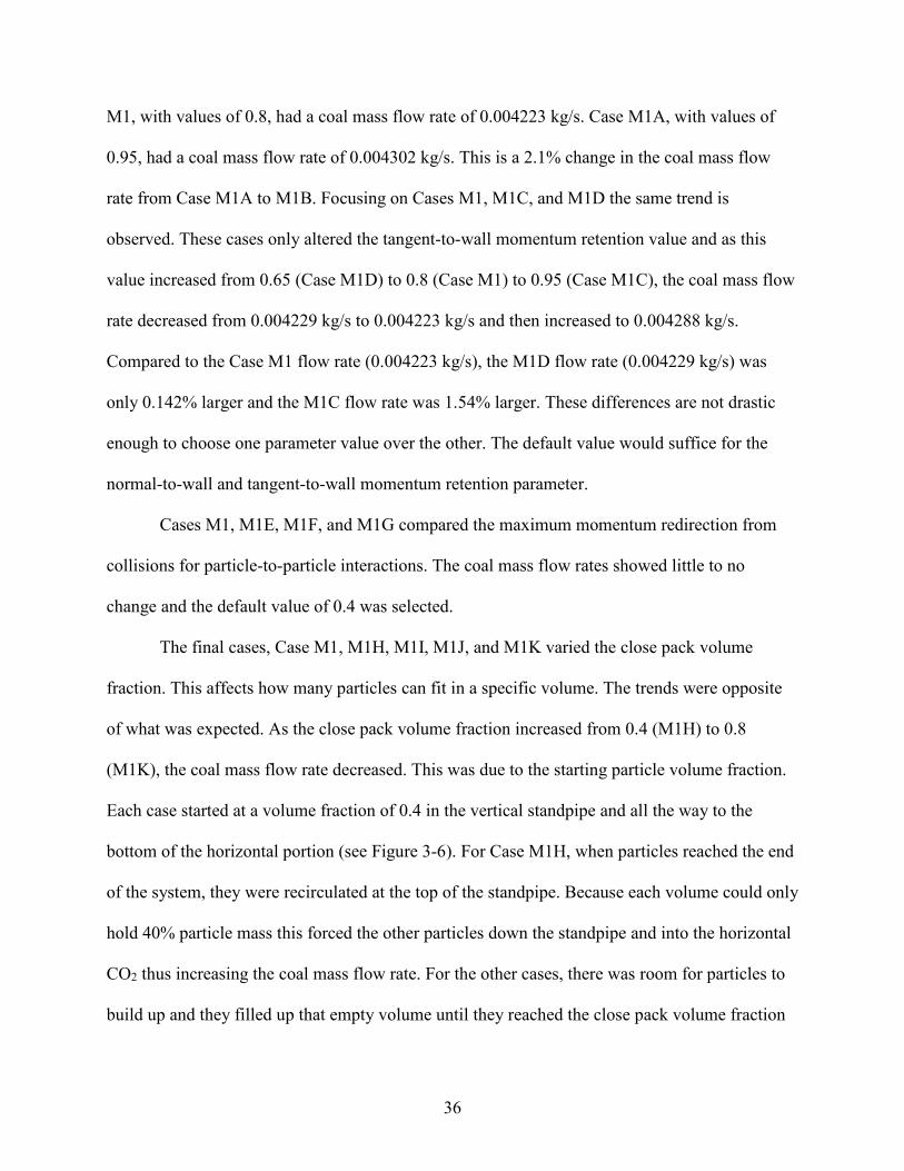
36

M1, with values of 0.8, had a coal mass flow rate of 0.004223 kg/s. Case M1A, with values of

0.95, had a coal mass flow rate of 0.004302 kg/s. This is a 2.1% change in the coal mass flow

rate from Case M1A to M1B. Focusing on Cases M1, M1C, and M1D the same trend is

observed. These cases only altered the tangent-to-wall momentum retention value and as this

value increased from 0.65 (Case M1D) to 0.8 (Case M1) to 0.95 (Case M1C), the coal mass flow

rate decreased from 0.004229 kg/s to 0.004223 kg/s and then increased to 0.004288 kg/s.

Compared to the Case M1 flow rate (0.004223 kg/s), the M1D flow rate (0.004229 kg/s) was

only 0.142% larger and the M1C flow rate was 1.54% larger. These differences are not drastic

enough to choose one parameter value over the other. The default value would suffice for the

normal-to-wall and tangent-to-wall momentum retention parameter.

Cases M1, M1E, M1F, and M1G compared the maximum momentum redirection from

collisions for particle-to-particle interactions. The coal mass flow rates showed little to no

change and the default value of 0.4 was selected.

The final cases, Case M1, M1H, M1I, M1J, and M1K varied the close pack volume

fraction. This affects how many particles can fit in a specific volume. The trends were opposite

of what was expected. As the close pack volume fraction increased from 0.4 (M1H) to 0.8

(M1K), the coal mass flow rate decreased. This was due to the starting particle volume fraction.

Each case started at a volume fraction of 0.4 in the vertical standpipe and all the way to the

bottom of the horizontal portion (see Figure 3-6). For Case M1H, when particles reached the end

of the system, they were recirculated at the top of the standpipe. Because each volume could only

hold 40% particle mass this forced the other particles down the standpipe and into the horizontal

CO2 thus increasing the coal mass flow rate. For the other cases, there was room for particles to

build up and they filled up that empty volume until they reached the close pack volume fraction

37

limit or reached the bottom of the vertical standpipe and then went on to flow with the horizontal

CO2.

After turning off the recirculation boundary condition connection, Cases M1, M1H, and

M1K were re-run to test if the cause of the increased coal mass flow rates were due to the

recirculation boundary condition. Case M1nr is similar to Case M1, Case M1Hnr is similar to

Case M1H, and Case M1Knr is similar to Case M1K. The difference between each of the cases

are that the original cases (M1, M1H, M1K) utilized the recirculation boundary condition and the

second set of cases (M1nr, M1Hnr, M1Knr) did not utilize the recirculation boundary condition.

Hence, the ‘nr’ means ‘no recirculation.’ Table 3-3 summarizes the results from these three cases

that were re-run and compares the results to the recirculation cases with the same model settings.

To reemphasize, Case M1nr had a close pack volume fraction of 0.6, Case M1Hnr had a close

pack volume fraction of 0.4, and Case M1Knr had a close pack volume fraction of 0.8. There are

slight changes to the coal mass flow rate between each of these cases, but not nearly as drastic of

change when compared to the previous cases with the recirculation boundary condition. There is

a 4.6% decrease in the coal mass flow rate comparing Case M1nr to Case M1Hnr and a 14.7%

decrease when comparing the coal mass flow rates for Case M1nr to Case M1Knr. From these

no-recirculation-cases, it is clear that the close pack volume fraction does not have a significant

effect on the coal mass flow rate for particles falling down a vertical pipe and into a horizontal

flow. The recirculation boundary condition however, does have an effect and will result in an

overestimate (by an order of magnitude) of the coal mass flow rate.

The average mass flow rate for Cases M1 through M1G (Table 3-2) was 0.004246 kg/s

with a standard deviation of the sample being 3.19 E-5 kg/s. The mass flow rates did not change

by more than 1.88% and this shows that a change in the sub-model parameters do not have a

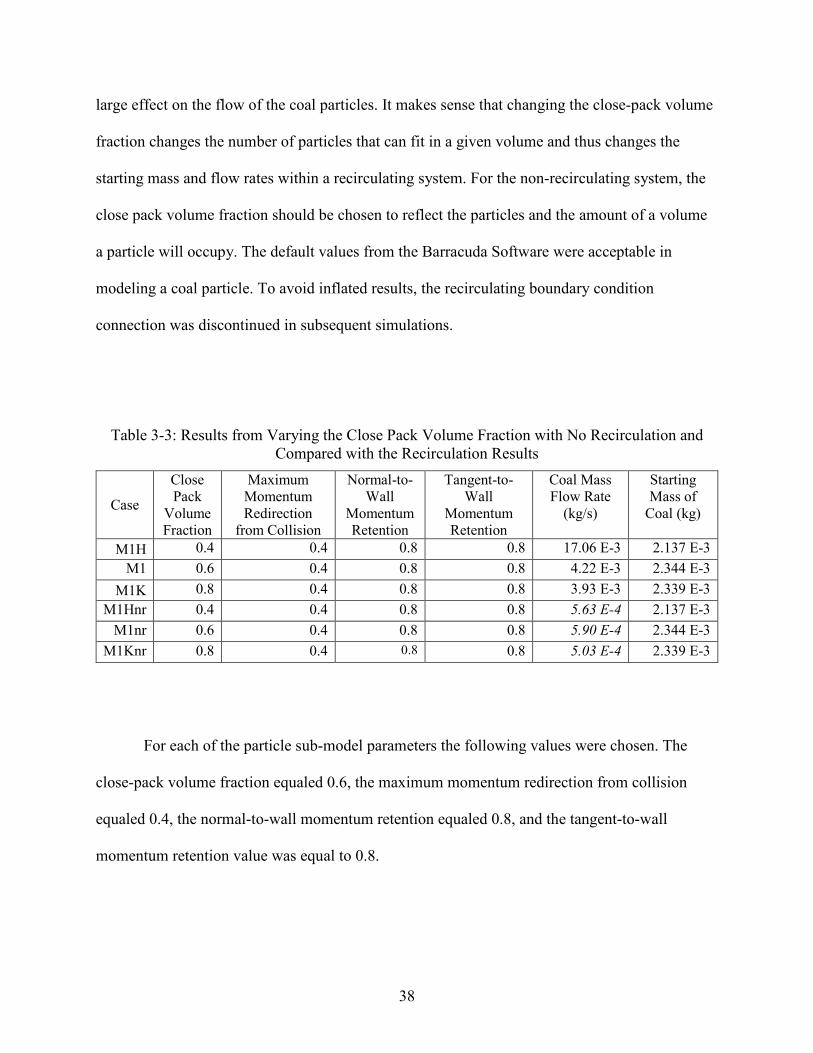
38

large effect on the flow of the coal particles. It makes sense that changing the close-pack volume

fraction changes the number of particles that can fit in a given volume and thus changes the

starting mass and flow rates within a recirculating system. For the non-recirculating system, the

close pack volume fraction should be chosen to reflect the particles and the amount of a volume

a particle will occupy. The default values from the Barracuda Software were acceptable in

modeling a coal particle. To avoid inflated results, the recirculating boundary condition

connection was discontinued in subsequent simulations.

Table 3-3: Results from Varying the Close Pack Volume Fraction with No Recirculation and Compared with the Recirculation Results

Case

Close Pack

Volume Fraction

Maximum Momentum Redirection

from Collision

Normal-to-Wall

Momentum Retention

Tangent-to-Wall

Momentum Retention

Coal Mass Flow Rate

(kg/s)

Starting Mass of

Coal (kg)

M1H 0.4 0.4 0.8 0.8 17.06 E-3 2.137 E-3 M1 0.6 0.4 0.8 0.8 4.22 E-3 2.344 E-3

M1K 0.8 0.4 0.8 0.8 3.93 E-3 2.339 E-3 M1Hnr 0.4 0.4 0.8 0.8 5.63 E-4 2.137 E-3

M1nr 0.6 0.4 0.8 0.8 5.90 E-4 2.344 E-3 M1Knr 0.8 0.4 0.8 0.8 5.03 E-4 2.339 E-3

For each of the particle sub-model parameters the following values were chosen. The

close-pack volume fraction equaled 0.6, the maximum momentum redirection from collision

equaled 0.4, the normal-to-wall momentum retention equaled 0.8, and the tangent-to-wall

momentum retention value was equal to 0.8.

39

3.5 Sampling Rate and Averaging

A sampling rate and averaging analysis was performed on one of the cases for the

fluidized bed system. The original data for the coal mass flow rate versus time obtained from

Barracuda is shown in Figure 3-8. When a case is running in Barracuda, it typically captures over

10,000 data points a second depending on the time step. This varies case to case depending on

the number of particles in the system, the type of flow, the boundary conditions, and the initial

conditions. With taking such a large number of data points, it is clear that nearly every

fluctuation in the coal mass flow rate will be recorded and this can be seen in Figure 3-8. This

portrays the flow rate of the coal exiting the pipe as it changes with time. Whenever there is a

significant increase of coal leaving the system, this is shown by a spike in the flow rate. In a

solid fuel combustion system, flames are sensitive to changes in burner coal flow on a time scale

of approximately one-second intervals. Fluctuations occurring at shorter times tend to be

averaged in the combustion process. To better assess the simulation fluctuations in context of

burner behavior, the data has been time-averaged, reducing the 10,000 data points a second to

one or two data points a second. This time-averaging technique provides a more useful

representation of how a burner would respond to variations in coal flow rate. The results show a

steadier flow of coal that fluctuates less with time. A steady flow in this comparison is a flow

that has the flow rate standard deviation over the flow rate average being less than or equal to

5%, or 0.05.

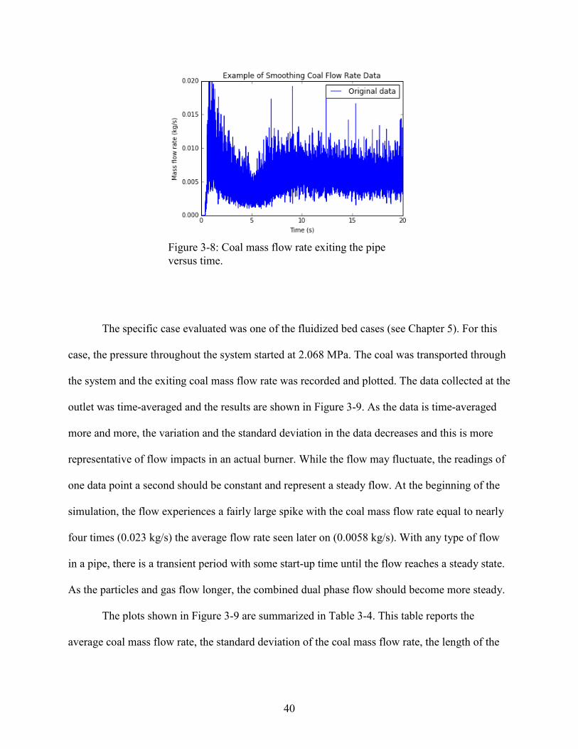
40

The specific case evaluated was one of the fluidized bed cases (see Chapter 5). For this

case, the pressure throughout the system started at 2.068 MPa. The coal was transported through

the system and the exiting coal mass flow rate was recorded and plotted. The data collected at the

outlet was time-averaged and the results are shown in Figure 3-9. As the data is time-averaged

more and more, the variation and the standard deviation in the data decreases and this is more

representative of flow impacts in an actual burner. While the flow may fluctuate, the readings of

one data point a second should be constant and represent a steady flow. At the beginning of the

simulation, the flow experiences a fairly large spike with the coal mass flow rate equal to nearly

four times (0.023 kg/s) the average flow rate seen later on (0.0058 kg/s). With any type of flow

in a pipe, there is a transient period with some start-up time until the flow reaches a steady state.

As the particles and gas flow longer, the combined dual phase flow should become more steady.

The plots shown in Figure 3-9 are summarized in Table 3-4. This table reports the

average coal mass flow rate, the standard deviation of the coal mass flow rate, the length of the

Figure 3-8: Coal mass flow rate exiting the pipe versus time.

41

new averaged vector, and the ratio of the standard deviation of the flow rate (STD) over the

average flow rate (AVG).

Table 3-4: Averaged-Down Data of a Fluidized Bed Case

Averaged Average Coal Mass Flow Rate (kg/s)

Standard Deviation Coal Flow (kg/s)

Length of Flow Rate Vector

STD/AVG (%)

No average 5.7575 E-3 1.4334 E-3 110399 24.90 10-point average 5.7573 E-3 1.3392 E-3 11040 23.26

100-point average 5.7577 E-3 0.8310 E-3 1104 14.43 1000-point average 5.7576 E-3 0.2137 E-3 111 3.71

10000-point average 5.7604 E-3 0.1320 E-3 12 2.29

Figure 3-9: All plots are exiting coal mass flow rate with respect to time. Top-left: averaging every 10 points. Top-right: averaging every 100 points. Bottom-left: averaging every 1000 points. Bottom-right: averaging every 10000 points.

42

For each simulation, two groups of data were averaged-down. For the plots, the data

ranging from the beginning to the end of the simulation was averaged-down and the average in

the left column signifies how many data points in the original data were combined to create the

new data set. In this case the simulation lasted 20 seconds. The second group of data refers to the

flow rates, standard deviations, and the length of the flow rate vector. This data was averaged

and taken from the time range where the flow visually leveled out and doing this omitted the

large spike and or dip in the flow rate at the beginning of the flow. For this case the averaged

were taken from 10-20 seconds. For all simulations, the averages were taken at the seemingly

steady state conditions in the flow.

43

4 GRAVITY-FED SYSTEM

This chapter discusses and analyzes the results of simulations of the gravity-fed system,

as previously introduced in Chapter 3 Model Development.

4.1 Initial Gravity-Fed Design

In addition to the mesh sensitivity and sub-model parameter studies completed with the

gravity-fed design, several additional parameters were studied including sphericity, particle

sizes, different pressures, incoming flow rates of the CO2. The sphericity results are summarized

in Table 4-1 and the particle sizes results are summarized in Table 4-2.

Table 4-1: Results of Sphericity Tests

Case Sphericity CO2 Mass Flow Rate (kg/s)

Coal Mass Flow Rate (kg/s)

Time to Empty* (s)

Starting Mass (kg)

CO2/Coal Mass Ratio

G1 1.0 0.004 5.90E-04 3.999 2.34E-03 6.778 G2 0.9 0.004 5.77E-04 4.043 2.34E-03 6.930 G3 0.8 0.004 5.75E-04 4.147 2.34E-03 6.955 G4 0.7 0.004 5.59E-04 4.194 2.34E-03 7.158 G5 0.6 0.004 5.77E-04 4.108 2.34E-03 6.928

*When mass in pipe gets below 2E-7 kg

44

As the sphericity decreased, the coal mass flow rates slightly decreased, but not

significantly. From the sphericity equal to 1 (Case G1) to a sphericity equal to 0.7 (Case G4), the

coal mass flow rate decreased by 5.25% (5.90E-4 kg/s to 5.59E-4 kg/s). Because of this decrease

in the flow rate, the time to empty the system slight increased from 3.999 seconds to 4.194

seconds, an increase of 4.65%. These changes in mass flow rates and the time to empty are not

drastic if each of these feed systems were to act as the operating feed system. However, the CO2-

to-coal mass ratio ranged from 6.778 to 7.158 which is too high for the targeted operational

region for the reactor.

Table 4-2: Gravity-Fed System Results with Varying Diameter Case Diameter

(µm) CO2 Mass Flow

Rate (kg/s) Coal Mass Flow

Rate (kg/s) Time to

Empty* (s) Starting

Mass (kg) CO2/Coal

Mass Ratio G6 125 0.004 7.86E-04 2.968 2.25E-03 5.091 G7 100 0.004 6.87E-04 3.405 2.27E-03 5.823 G1 75 0.004 5.90E-04 3.999 2.34E-03 6.778 G8 50 0.004 4.27E-04 5.059 2.17E-03 9.368 G9 25 0.004 2.42E-04 9.435 2.15E-03 16.544

*When mass in pipe gets below 2E-7 kg

As the coal particle diameter decreased, the coal mass flow rate also decreased. This is

due to the change in mass. The bigger, or more massive particles dropped faster from the vertical

standpipe into the horizontal pipe than the smaller, or less massive particles. This is reflected in

the time it took to empty the system; as the particle size decreases, the time to empty the system

increases. The larger 125-µm particle had a volume (and mass) 125-times larger than the smaller

45

25-µm particle. To maintain the same flow rate of particles, 125 of the smaller particles would

need to exit the system for every one of the larger particles.

Table 4-3 summarizes the results of CO2 and coal flow with changes in pressure. At a

high pressure of 2 MPa and a CO2 mass flow rate of 0.004 kg/s there is too much CO2 and not

enough coal flowing out the exit (0.0005901 kg/s). The CO2 mass flow rate was rounded to

0.004 kg/s for these simulations from 0.00378 kg/s. This made future percentage increases and

decreases CO2 mass flow rates more convenient. The ratio of the CO2 mass flow rate over the

coal mass flow rate was equal to 6.8 and this was too high for the reactor. A fuel lean

equivalence ratio is desired for combustion (CO2-to-coal ratio greater than one), but since

additional gas is added via other burner inlets, the gas mass flow rate associated with coal

transport must be limited to 1-2 times the coal flow rate. Not only was the ratio excessively fuel

lean, but the coal mass flow rate was a sixth of the targeted flow rate. A coal flow rate of

0.00378 kg/s was targeted for baseline operation. The coal flow rate can fluctuate, but with the

equivalence ratio always staying lean, the combustion of coal should always be complete. At 2

MPa the gravity-fed system could not meet this ratio with the required amount of coal mass flow

rate and a new design was needed. As seen from Table 4-3, at 0.1 MPa on the first row, last

column, the ratio was a little lower than 3-to-1 and this was closer to the desired operating ratio.

As the pressure increases from atmospheric pressure (0.1 MPa) to the reactor operating pressure

(2.0 MPa), the CO2-to-coal mass flow ratios increases, which is not practicable for the reactor.

This implies that this system could be feasible at an atmospheric pressure (0.1 MPa), but at a

higher pressure (2 MPa), another design is needed.

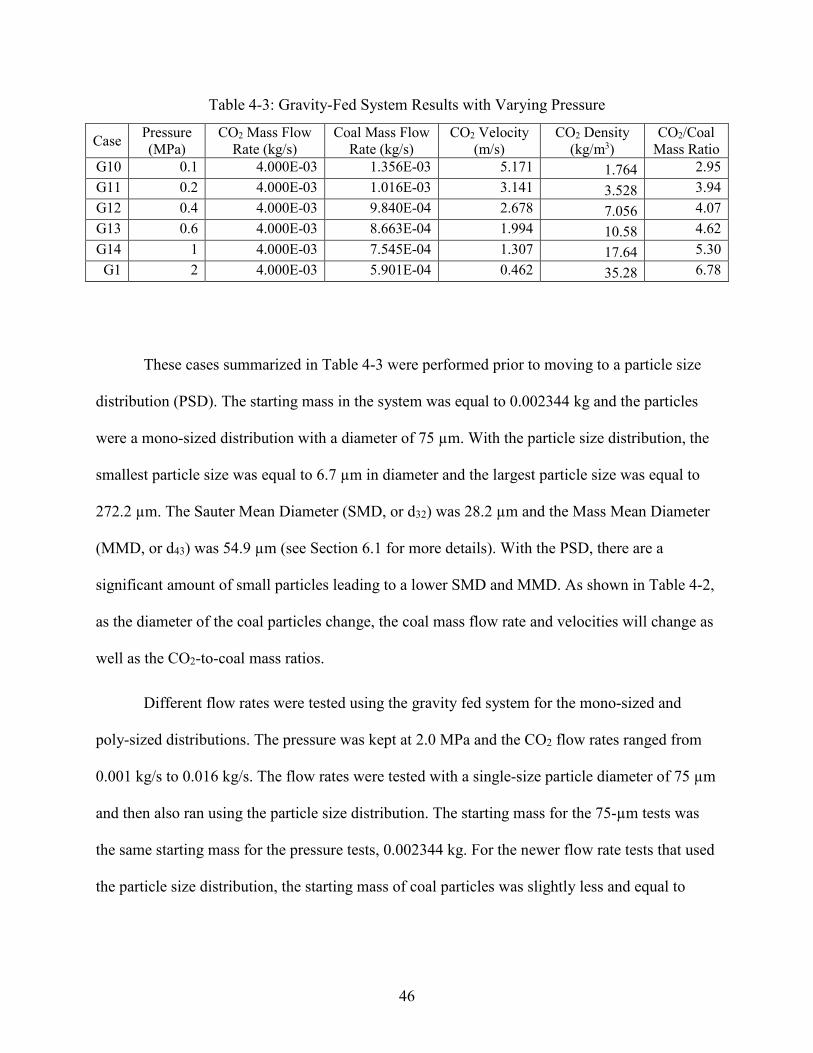
46

Table 4-3: Gravity-Fed System Results with Varying Pressure

These cases summarized in Table 4-3 were performed prior to moving to a particle size

distribution (PSD). The starting mass in the system was equal to 0.002344 kg and the particles

were a mono-sized distribution with a diameter of 75 µm. With the particle size distribution, the

smallest particle size was equal to 6.7 µm in diameter and the largest particle size was equal to

272.2 µm. The Sauter Mean Diameter (SMD, or d32) was 28.2 µm and the Mass Mean Diameter

(MMD, or d43) was 54.9 µm (see Section 6.1 for more details). With the PSD, there are a

significant amount of small particles leading to a lower SMD and MMD. As shown in Table 4-2,

as the diameter of the coal particles change, the coal mass flow rate and velocities will change as

well as the CO2-to-coal mass ratios.

Different flow rates were tested using the gravity fed system for the mono-sized and

poly-sized distributions. The pressure was kept at 2.0 MPa and the CO2 flow rates ranged from

0.001 kg/s to 0.016 kg/s. The flow rates were tested with a single-size particle diameter of 75 µm

and then also ran using the particle size distribution. The starting mass for the 75-µm tests was

the same starting mass for the pressure tests, 0.002344 kg. For the newer flow rate tests that used

the particle size distribution, the starting mass of coal particles was slightly less and equal to

Case Pressure (MPa)

CO2 Mass Flow Rate (kg/s)


CO2 Velocity (m/s)

CO2 Density (kg/m3)

CO2/Coal Mass Ratio

G10 0.1 4.000E-03 1.356E-03 5.171 1.764 2.95 G11 0.2 4.000E-03 1.016E-03 3.141 3.528 3.94 G12 0.4 4.000E-03 9.840E-04 2.678 7.056 4.07 G13 0.6 4.000E-03 8.663E-04 1.994 10.58 4.62 G14 1 4.000E-03 7.545E-04 1.307 17.64 5.30

G1 2 4.000E-03 5.901E-04 0.462 35.28 6.78

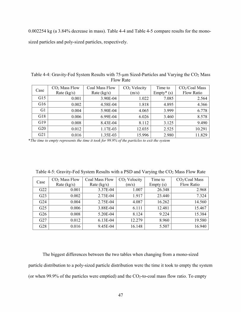
47

0.002254 kg (a 3.84% decrease in mass). Table 4-4 and Table 4-5 compare results for the mono-

sized particles and poly-sized particles, respectively.

Table 4-4: Gravity-Fed System Results with 75-µm Sized-Particles and Varying the CO2 Mass Flow Rate

Case CO2 Mass Flow Rate (kg/s)


CO2 Velocity (m/s)

Time to Empty* (s)

CO2/Coal Mass Flow Ratio

G15 0.001 3.90E-04 1.022 7.085 2.564 G16 0.002 4.58E-04 1.818 4.895 4.366 G1 0.004 5.90E-04 4.065 3.999 6.778

G18 0.006 6.99E-04 6.026 3.460 8.578 G19 0.008 8.43E-04 8.112 3.125 9.490 G20 0.012 1.17E-03 12.035 2.525 10.291 G21 0.016 1.35E-03 15.996 2.980 11.829

*The time to empty represents the time it took for 99.9% of the particles to exit the system

Table 4-5: Gravity-Fed System Results with a PSD and Varying the CO2 Mass Flow Rate



CO2 Velocity (m/s)

Time to Empty (s)

CO2/Coal Mass Flow Ratio

G22 0.001 3.37E-04 1.007 26.348 2.968 G23 0.002 2.73E-04 1.917 23.440 7.324 G24 0.004 2.75E-04 4.087 16.262 14.560 G25 0.006 3.88E-04 6.111 12.481 15.467 G26 0.008 5.20E-04 8.124 9.224 15.384 G27 0.012 6.13E-04 12.279 8.960 19.580 G28 0.016 9.45E-04 16.148 5.507 16.940

The biggest differences between the two tables when changing from a mono-sized

particle distribution to a poly-sized particle distribution were the time it took to empty the system

(or when 99.9% of the particles were emptied) and the CO2-to-coal mass flow ratio. To empty

48

the system for the gravity-fed system, for a CO2 mass flow rate of 0.004 kg/s and system

pressure of 2 MPa, took a little over 16 seconds. If the flow rate was faster, it took less time to

empty the system. The cases that were ran in Table 4-5 used the poly-sized distribution and this

led to longer times to empty the particles. The cases that had the same flow rates were compared

to each other and the results in Figure 4-1 were consistent in that the cases with the particle size

distribution took longer to empty the system. This is because there were smaller particles for the

tests running with the poly-sized distribution for the particle sizes. This agrees with previous

tests (see Table 4-2) that when changing the overall diameter of the particles, the time to empty

the system will change.

For the 75-µm diameter particles, as the CO2 mass flow rate increased from 0.001 kg/s to

0.016 kg/s the CO2-to-coal mass ratio increased in a constant manner from 2.56 to 11.83. For the

PSD, the same changes in the CO2 mass flow rate from 0.001 kg/s to 0.016 kg/s increased the

CO2-to-coal mass ratio in a less constant manner from 2.97 to 16.94. For the PSD, when the CO2

flow rate was 0.004 kg/s, the CO2-to-coal mass ratio was already 14.56. Comparing this to the

75-µm diameter results at a CO2 flow rate of 0.004 kg/s, the CO2-to-coal mass ratio was only

6.78. The CO2-to-coal mass ratio increased quickly for the PSD cases then leveled off at a high

ratio as the CO2 flow rate increased. This ratio leveled off because of the rate at which the

particles dropped into the flow from the vertical standpipe. The higher CO2 flow rates had

slightly higher coal mass flow rates, but not a significant amount. The smaller particles, due to a

lower body force in the PSD, were unable to overcome the cohesion forces in the standpipe,

dropped at a lower rate, and this led to lower coal mass flow rates when compared to the cases

implementing the 75-µm diameter particles.

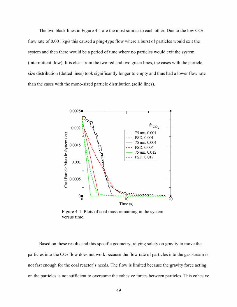
49

The two black lines in Figure 4-1 are the most similar to each other. Due to the low CO2

flow rate of 0.001 kg/s this caused a plug-type flow where a burst of particles would exit the

system and then there would be a period of time where no particles would exit the system

(intermittent flow). It is clear from the two red and two green lines, the cases with the particle

size distribution (dotted lines) took significantly longer to empty and thus had a lower flow rate

than the cases with the mono-sized particle distribution (solid lines).

Based on these results and this specific geometry, relying solely on gravity to move the

particles into the CO2 flow does not work because the flow rate of particles into the gas stream is

not fast enough for the coal reactor’s needs. The flow is limited because the gravity force acting

on the particles is not sufficient to overcome the cohesive forces between particles. This cohesive

Figure 4-1: Plots of coal mass remaining in the system versus time.

50

effect is increased by the high pressure in the system. Any potential entrainment effect by the gas

stream is mitigated by the relatively low velocities (3.38 m/s). In addition to the limited flow

rates, the gravity-fed design is more prone to bridging and ratholing which could cause

intermittent flow or stop the flow of coal indefinitely.

4.2 Modified Gravity-Fed Design

In an attempt to improve the flow of coal from the hopper to the horizontal pipe, a

modified gravity-fed geometry was created turning the vertical standpipe into an angled conical

shape as shown in Figure 4-2. Table 4-6 summarizes the results and this design also proved to be

unsuccessful at supplying a sufficient, steady, and uniform flow of coal out of the system. Coal

particles with the same PSD of approximately the same mass (0.002233 kg) as the original

gravity-fed system was added to the hopper with a little gap between the top of the coal and the

top of the geometry. The gap at the top of the hopper was introduced to allow the particles space

to fluidize in the hopper to introduce more coal into the flow of incoming horizontal CO2.

Figure 4-2: Geometry of the angled hopper with the same amount of mass and same boundary and initial conditions as the original gravity-fed system discussed in Section 4.1.

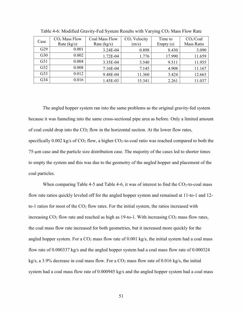
51

Table 4-6: Modified Gravity-Fed System Results with Varying CO2 Mass Flow Rate



CO2 Velocity (m/s)

Time to Empty (s)

CO2/Coal Mass Ratio

G29 0.001 3.24E-04 0.898 8.430 3.090 G30 0.002 1.72E-04 1.776 17.990 11.659 G31 0.004 3.35E-04 3.540 9.511 11.955 G32 0.008 7.16E-04 7.145 4.908 11.167 G33 0.012 9.48E-04 11.360 3.424 12.663 G34 0.016 1.45E-03 15.341 2.261 11.037

The angled hopper system ran into the same problems as the original gravity-fed system

because it was funneling into the same cross-sectional pipe area as before. Only a limited amount

of coal could drop into the CO2 flow in the horizontal section. At the lower flow rates,

specifically 0.002 kg/s of CO2 flow, a higher CO2-to-coal ratio was reached compared to both the

75-µm case and the particle size distribution case. The majority of the cases led to shorter times

to empty the system and this was due to the geometry of the angled hopper and placement of the

coal particles.

When comparing Table 4-5 and Table 4-6, it was of interest to find the CO2-to-coal mass

flow rate ratios quickly leveled off for the angled hopper system and remained at 11-to-1 and 12-

to-1 ratios for most of the CO2 flow rates. For the initial system, the ratios increased with

increasing CO2 flow rate and reached as high as 19-to-1. With increasing CO2 mass flow rates,

the coal mass flow rate increased for both geometries, but it increased more quickly for the

angled hopper system. For a CO2 mass flow rate of 0.001 kg/s, the initial system had a coal mass

flow rate of 0.000337 kg/s and the angled hopper system had a coal mass flow rate of 0.000324

kg/s, a 3.9% decrease in coal mass flow. For a CO2 mass flow rate of 0.016 kg/s, the initial

system had a coal mass flow rate of 0.000945 kg/s and the angled hopper system had a coal mass

52

flow rate of 0.00145 kg/s, a 34.8% increase in the coal mass flow. At the higher flow rates, the

angled hopper system is more effective and moving coal through the piping, but still does not

meet the coal flow rate of 0.00378 kg/s and CO2-to-coal mass ratio requirements of the range

from 1 to 2.

An important comparison is shown regarding the two different gravity-fed systems in

Figure 4-3. The top portion of each image shows the junction of where the particles drop down

from the vertical section into the horizontal section. It is seen for the vertical standpipe that the

particles drop about halfway into the horizontal section and are immediately transported by the

CO2 to the right. For the angled cone hopper, the particles do not drop down as far and are taken

quicker into the horizontal flow than the vertical standpipe orientation. With approximately the

same mass remaining above the intersection of the vertical and horizontal sections of the pipe

and the same mass flow rates, the differences are surprising between the two simulations. The

bottom portion of the image shows where coal particles are leaving. It can be seen that the

particles after 30 cm of traveling horizontally begin to group on the bottom of the pipe.

Figure 4-3: The initial gravity-fed geometry is shown in the top image and the particles are shown mid-simulation. The modified geometry with the angled conical hopper is shown in the bottom image with the particles also shown mid-simulation. The operating pressure was 2.0 MPa and the CO2 mass flow rate was 0.004 kg/s

53

In summary, neither of the gravity-fed systems were able to meet the desired performance

requirements of coal mass flow rate and CO2-to-coal flow mass ratio. This geometry was tested

as a simple concept to determine if it would deliver the appropriate coal mass flow rate and gas-

to-particle mass ratios. Other gravity-fed designs may be able to satisfy the design requirements

but the complexity of the system will increase with the addition of pipe diameter changes,

eductors, etc. Passing no gas flow through the hopper also increases the risk of coal clogging or

bridging in the real system hopper.

54

5 FLUIDIZED BED SYSTEM

This chapter discusses the fluidized bed system as portrayed in Figure 5-1. For this

design concept, the particles are put in a large hopper or bed, the bed is pressurized and then

fluidized with CO2 entering the hopper through Inlet A and a fraction of that CO2 is allowed to

exit through Outlet C. The CO2 and fluidized particles are transported out of the hopper and into

the horizontal pipe, Pipe E. By fluidizing the hopper, this provides a steady flow of CO2 and coal

leaving the hopper through Pipe E. This system is flexible because of an additional inlet of CO2,

Inlet B. This is referred to as the dilution flow because based on the mass flow ratio of CO2-to-

coal leaving the hopper through Pipe E, the ratio can be adjusted to what the reactor requires by

changing Inlet B and its CO2 mass flow rate. Outlet D represents the end of this system and

continues on to the reactor. The coal and CO2 mass flow rates and ratios reported in this chapter

were measured at Outlet D. This fluidized bed design concept was developed in response to the

restricted coal flow rates observed in the gravity-fed system. The goal of the design was to

improve the flow rate of coal by fluidizing the particles before transporting them, thus reducing

the cohesive or packing forces limiting particle flow.

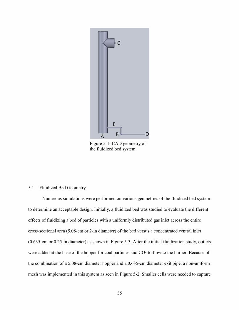
55

5.1 Fluidized Bed Geometry

Numerous simulations were performed on various geometries of the fluidized bed system

to determine an acceptable design. Initially, a fluidized bed was studied to evaluate the different

effects of fluidizing a bed of particles with a uniformly distributed gas inlet across the entire

cross-sectional area (5.08-cm or 2-in diameter) of the bed versus a concentrated central inlet

(0.635-cm or 0.25-in diameter) as shown in Figure 5-3. After the initial fluidization study, outlets

were added at the base of the hopper for coal particles and CO2 to flow to the burner. Because of

the combination of a 5.08-cm diameter hopper and a 0.635-cm diameter exit pipe, a non-uniform

mesh was implemented in this system as seen in Figure 5-2. Smaller cells were needed to capture

Figure 5-1: CAD geometry of the fluidized bed system.

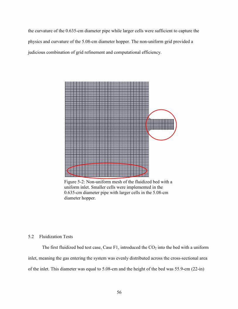
56

the curvature of the 0.635-cm diameter pipe while larger cells were sufficient to capture the

physics and curvature of the 5.08-cm diameter hopper. The non-uniform grid provided a

judicious combination of grid refinement and computational efficiency.

5.2 Fluidization Tests

The first fluidized bed test case, Case F1, introduced the CO2 into the bed with a uniform

inlet, meaning the gas entering the system was evenly distributed across the cross-sectional area

of the inlet. This diameter was equal to 5.08-cm and the height of the bed was 55.9-cm (22-in)

Figure 5-2: Non-uniform mesh of the fluidized bed with a uniform inlet. Smaller cells were implemented in the 0.635-cm diameter pipe with larger cells in the 5.08-cm diameter hopper.

57

with the center of the 0.635-cm diameter outlet being 6.35-cm away from the top of the system.

The mass flow rate of CO2 was equal to 0.004 kg/s, the pressure was equal to 2.0 MPa, yielding

a CO2 density of 35.28 kg/m3 and a velocity of 0.0559 m/s. This velocity is well above the

minimum bubbling velocity and close to the minimum slugging velocity [7]. This ensured that

the bed was fluidized and no bridging would occur. All gas flow entering from the bottom of the

bed exited through the horizontal outlet at the top of the hopper. Snapshots of the flow were

taken every second from zero to seven seconds and the results are shown in Figure 5-4.

Figure 5-3: Two geometries used to test fluidization: Uniform inlet (left, Case F1) and concentrated central inlet (right, Case F2).

Inlet

Outlet

40°

58

After about five seconds, the flow seems to be steady based on the consistent particle

volume fraction between seconds 5, 6, and 7. The particles have been lifted up in the bed well

past the outlet and are close to the top of the system and will remain suspended because of the

incoming CO2 mass flow rate. At the inlet, the particles are all lifted up for a couple centimeters

and on the far right side, the particle volume fraction remains about half (0.3) of what the particle

volume fraction is in the rest of the system (0.6). The pressure drop from the inlet to the outlet

was constantly increasing. At two seconds, the pressure drop was 0.258 MPa. At four seconds,

the pressure drop was 0.626 MPa. At six seconds, the pressure drop was 0.809 MPa. At eight

seconds, the pressure drop was 0.867 MPa. And at ten seconds, the pressure drop was 1.035

MPa. The system started at 2.0 MPa and after 10 seconds, the maximum pressure reached 3.57

Figure 5-4: Inside look (geometry cut in half) at the particle volume fraction in the first geometry looking at fluidization and the particle characteristics every second from zero to seven seconds.

59

MPa a 78.5% increase of pressure. This was caused by the small size of the outlet for CO2 to

leave the system. CO2 was building up in the system and thus increased the pressure by nearly

doubling it in the course of ten seconds.

The case, Case F1, was re-run with a larger outlet for the CO2. This was a pressure

boundary condition and at the end of the first run, the final pressure was equal to 2.54 MPa when

it should have been equal to 2.0 MPa. For the repeat case, but with the better pressure boundary

condition, the final pressure was equal to 2.00 MPa, as expected and the more accurate results

are shown in Figure 5-5. The pressure drop across the fluidized bed was equal to 0.379 MPa, and

while this was a large decrease from the previous case, this was still a significant pressure drop

across a fluidized bed. This large pressure buildup is due to the transient period in the beginning

of the simulation. In the geometry, there is one inlet and one outlet. It is straight forward in that

the CO2 coming into the system should also be leaving the system. Due to compressibility

effects, the CO2 built up and increased the pressure in the first few seconds of the simulation.

After about 5 seconds of simulating, the CO2 exiting the system equaled the CO2 entering the

system and the pressure was stable.

Figure 5-5 shows the fluidization of coal particles. The CO2 prefers to travel up the walls

of the hopper and this can be seen from the bottom of the hopper where the green colored

particles form a boundary and lower particle volume fraction on the walls. Compared to Figure

5-4, the particles are more fluidized in the bottom of the hopper and more densely packed in the

top of the hopper close to the outlet. If the hopper were taller, the particles would have continued

to expand as they fluidized. This test showed the bed was fluidized very well and this design

showed potential for fluidizing and transporting the particles effectively.

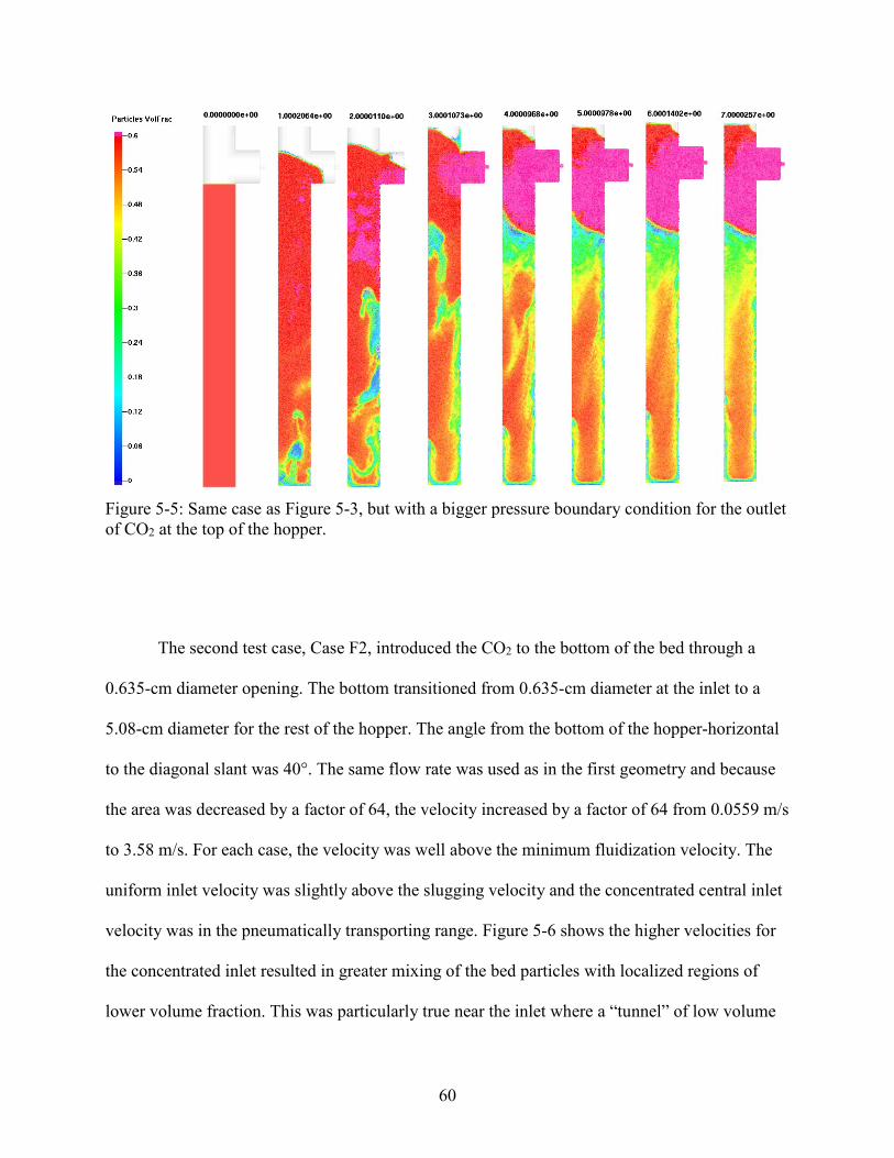
60

The second test case, Case F2, introduced the CO2 to the bottom of the bed through a

0.635-cm diameter opening. The bottom transitioned from 0.635-cm diameter at the inlet to a

5.08-cm diameter for the rest of the hopper. The angle from the bottom of the hopper-horizontal

to the diagonal slant was 40°. The same flow rate was used as in the first geometry and because

the area was decreased by a factor of 64, the velocity increased by a factor of 64 from 0.0559 m/s

to 3.58 m/s. For each case, the velocity was well above the minimum fluidization velocity. The

uniform inlet velocity was slightly above the slugging velocity and the concentrated central inlet

velocity was in the pneumatically transporting range. Figure 5-6 shows the higher velocities for

the concentrated inlet resulted in greater mixing of the bed particles with localized regions of

lower volume fraction. This was particularly true near the inlet where a “tunnel” of low volume

Figure 5-5: Same case as Figure 5-3, but with a bigger pressure boundary condition for the outlet of CO2 at the top of the hopper.

61

fraction particles formed, surrounded by higher volume fraction particles. A region of high

volume fraction particles still remained near the exit at the top of the hopper where expansion

was constricted. Overall, the bed was less uniformly fluidized and was characterized by larger

differences in particle volume fraction in different bed regions. The startup behavior in the bed

was also more turbulent due to the push of the high velocity gas through the particles. Overall,

the resulting fluidization state of the bed appeared less amenable to steady transport of particles

out of the hopper than with the uniform CO2 inlet design.

Figure 5-6: Look inside of the particle volume fraction for the second geometry, Case F2, (0.635-cm diameter inlet) every second from zero to seven seconds.

62

The majority of the bed was much more fluidized in the second case because of the smaller

area and higher velocity of the CO2. The particles were constantly mixing and filled up the

entirety of the geometry. At the beginning of the inlet the particles remained packed (red particle

volume fraction) on the sides of the hopper and the incoming jet of CO2 was concentrated in the

middle of the hopper, after approximately 10 cm the entire hopper was fluidized.

5.3 Fluidized Bed Designs

Once the fluidization was explored in the bed, an outlet was added near the bottom of the

bed. This outlet traveled horizontally, then vertically down, before merging into the main

horizontal transport pipe. A second gas inlet (B) shown in Figure 5-7 was added at the left of the

main horizontal transport pipe. The outlet of this system would then connect to the inlet of the

reactor via a piping system.

For the 5.08-cm diameter hopper (uniform inlet) operating at a pressure of 2 MPa, the

minimum fluidization velocity (from Equation 2-3) was equal to 4.72E-4 m/s and a minimum

fluidization flow rate equal to 3.38E-5 kg/s. After running this case, Case F3, with the minimum

fluidization flow rate, with all the CO2 coming in through Inlet A and leaving through Outlet D,

the exit coal mass flow rate was equal to 0.000669 kg/s giving a CO2-to-coal mass ratio of

0.0504. Compared to the gravity-fed system, where the coal flow rate was always less than the

CO2 flow rate, the fluidized bed system supplies a greater coal flow rate than CO2 flow rate. This

result showed that the fluidized bed concept was effective at moving relatively large amounts of

coal with minimal gas flow. This was very different from the gravity-fed design and confirmed

the initial objectives of the fluidized bed design.

63

The problem with this case, Case F3, where there is only Inlet A and Outlet D is that it

does not entirely fluidize the bed, but the CO2 immediately flows out of the hopper. Outlet C is

needed to fluidize the bed and ensure that clogging of the particles does not occur. Theoretically,

as assumed, the model will work if the coal particles have no moisture. In reality, the coal

particles are more cohesive and can stick together in a packed bed.

Figure 5-7: Modified geometry of the fluidized bed to test exiting coal mass flow rates and CO2-to-coal mass ratios. The uniform inlet (left) and concentrated central inlet (right) are shown.

Second Inlet

A A D D

E E

BB

C C

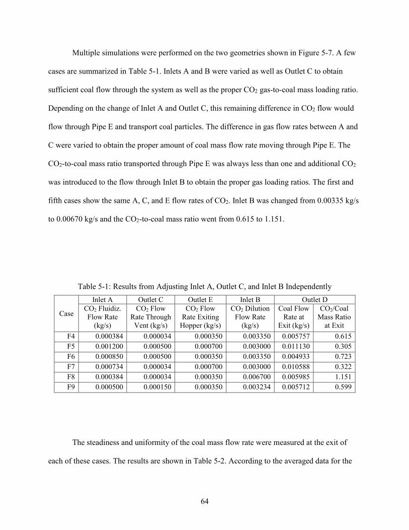
64

Multiple simulations were performed on the two geometries shown in Figure 5-7. A few

cases are summarized in Table 5-1. Inlets A and B were varied as well as Outlet C to obtain

sufficient coal flow through the system as well as the proper CO2 gas-to-coal mass loading ratio.

Depending on the change of Inlet A and Outlet C, this remaining difference in CO2 flow would

flow through Pipe E and transport coal particles. The difference in gas flow rates between A and

C were varied to obtain the proper amount of coal mass flow rate moving through Pipe E. The

CO2-to-coal mass ratio transported through Pipe E was always less than one and additional CO2

was introduced to the flow through Inlet B to obtain the proper gas loading ratios. The first and

fifth cases show the same A, C, and E flow rates of CO2. Inlet B was changed from 0.00335 kg/s

to 0.00670 kg/s and the CO2-to-coal mass ratio went from 0.615 to 1.151.

Table 5-1: Results from Adjusting Inlet A, Outlet C, and Inlet B Independently

Case

Inlet A Outlet C Outlet E Inlet B Outlet D CO2 Fluidiz. Flow Rate

(kg/s)

CO2 Flow Rate Through

Vent (kg/s)

CO2 Flow Rate Exiting

Hopper (kg/s)

CO2 Dilution Flow Rate

(kg/s)

Coal Flow Rate at

Exit (kg/s)

CO2/Coal Mass Ratio

at Exit F4 0.000384 0.000034 0.000350 0.003350 0.005757 0.615 F5 0.001200 0.000500 0.000700 0.003000 0.011130 0.305 F6 0.000850 0.000500 0.000350 0.003350 0.004933 0.723 F7 0.000734 0.000034 0.000700 0.003000 0.010588 0.322 F8 0.000384 0.000034 0.000350 0.006700 0.005985 1.151 F9 0.000500 0.000150 0.000350 0.003234 0.005712 0.599

The steadiness and uniformity of the coal mass flow rate were measured at the exit of

each of these cases. The results are shown in Table 5-2. According to the averaged data for the

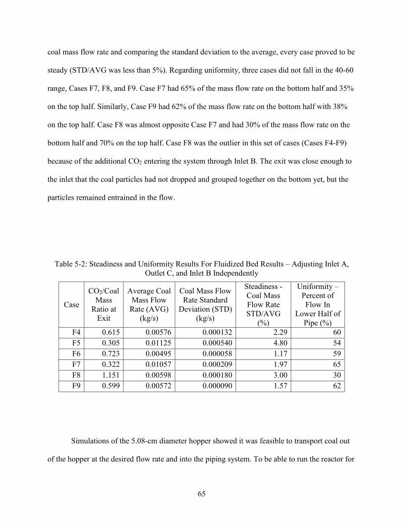
65

coal mass flow rate and comparing the standard deviation to the average, every case proved to be

steady (STD/AVG was less than 5%). Regarding uniformity, three cases did not fall in the 40-60

range, Cases F7, F8, and F9. Case F7 had 65% of the mass flow rate on the bottom half and 35%

on the top half. Similarly, Case F9 had 62% of the mass flow rate on the bottom half with 38%

on the top half. Case F8 was almost opposite Case F7 and had 30% of the mass flow rate on the

bottom half and 70% on the top half. Case F8 was the outlier in this set of cases (Cases F4-F9)

because of the additional CO2 entering the system through Inlet B. The exit was close enough to

the inlet that the coal particles had not dropped and grouped together on the bottom yet, but the

particles remained entrained in the flow.

Table 5-2: Steadiness and Uniformity Results For Fluidized Bed Results – Adjusting Inlet A, Outlet C, and Inlet B Independently

Case

CO2/Coal Mass

Ratio at Exit

Average Coal Mass Flow Rate (AVG)

(kg/s)

Coal Mass Flow Rate Standard

Deviation (STD) (kg/s)

Steadiness - Coal Mass Flow Rate STD/AVG

(%)

Uniformity – Percent of Flow In

Lower Half of Pipe (%)

F4 0.615 0.00576 0.000132 2.29 60 F5 0.305 0.01125 0.000540 4.80 54 F6 0.723 0.00495 0.000058 1.17 59 F7 0.322 0.01057 0.000209 1.97 65 F8 1.151 0.00598 0.000180 3.00 30 F9 0.599 0.00572 0.000090 1.57 62

Simulations of the 5.08-cm diameter hopper showed it was feasible to transport coal out

of the hopper at the desired flow rate and into the piping system. To be able to run the reactor for

66

hours at a time without having to refill the hopper, a larger 15.24-cm (6-in) diameter hopper was

tested as illustrated in Figure 5-8. These simulations focused on the fluidization behavior for

different gas inlet designs and so only included the lower portion of what would be a much taller

hopper in the actual pilot-scale design.

Cases of interest are recorded in Table 5-3. The cases with the 15-cm (15.24-cm)

diameter had a starting mass of 3.053 kg and the transitional 5-to-15-cm (5.08-to-15.24-cm)

diameter had a starting mass of 1.460 kg. The distance from the inlet to the outlet pipe, Pipe E

for the 15-cm diameter cases measured 7.62-cm and for the transitional 5-to-15-cm diameter

cases, this distance measured 5.08-cm. For the transitional 5-to-15-cm diameter cases, the angle

Figure 5-8: Geometries for the: a) 15-cm diameter hopper and b) the transitional 5-to-15-cm diameter hopper.

A A

C C

E

E D

D

a) b)

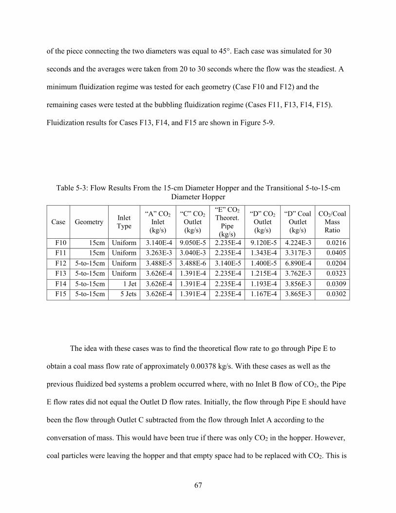
67

of the piece connecting the two diameters was equal to 45°. Each case was simulated for 30

seconds and the averages were taken from 20 to 30 seconds where the flow was the steadiest. A

minimum fluidization regime was tested for each geometry (Case F10 and F12) and the

remaining cases were tested at the bubbling fluidization regime (Cases F11, F13, F14, F15).

Fluidization results for Cases F13, F14, and F15 are shown in Figure 5-9.

Table 5-3: Flow Results From the 15-cm Diameter Hopper and the Transitional 5-to-15-cm Diameter Hopper

Case Geometry Inlet Type

“A” CO2 Inlet (kg/s)

“C” CO2 Outlet (kg/s)

“E” CO2 Theoret.

Pipe (kg/s)

“D” CO2 Outlet (kg/s)

“D” Coal Outlet (kg/s)

CO2/Coal Mass Ratio

F10 15cm Uniform 3.140E-4 9.050E-5 2.235E-4 9.120E-5 4.224E-3 0.0216 F11 15cm Uniform 3.263E-3 3.040E-3 2.235E-4 1.343E-4 3.317E-3 0.0405 F12 5-to-15cm Uniform 3.488E-5 3.488E-6 3.140E-5 1.400E-5 6.890E-4 0.0204 F13 5-to-15cm Uniform 3.626E-4 1.391E-4 2.235E-4 1.215E-4 3.762E-3 0.0323 F14 5-to-15cm 1 Jet 3.626E-4 1.391E-4 2.235E-4 1.193E-4 3.856E-3 0.0309 F15 5-to-15cm 5 Jets 3.626E-4 1.391E-4 2.235E-4 1.167E-4 3.865E-3 0.0302

The idea with these cases was to find the theoretical flow rate to go through Pipe E to

obtain a coal mass flow rate of approximately 0.00378 kg/s. With these cases as well as the

previous fluidized bed systems a problem occurred where, with no Inlet B flow of CO2, the Pipe

E flow rates did not equal the Outlet D flow rates. Initially, the flow through Pipe E should have

been the flow through Outlet C subtracted from the flow through Inlet A according to the

conversation of mass. This would have been true if there was only CO2 in the hopper. However,

coal particles were leaving the hopper and that empty space had to be replaced with CO2. This is

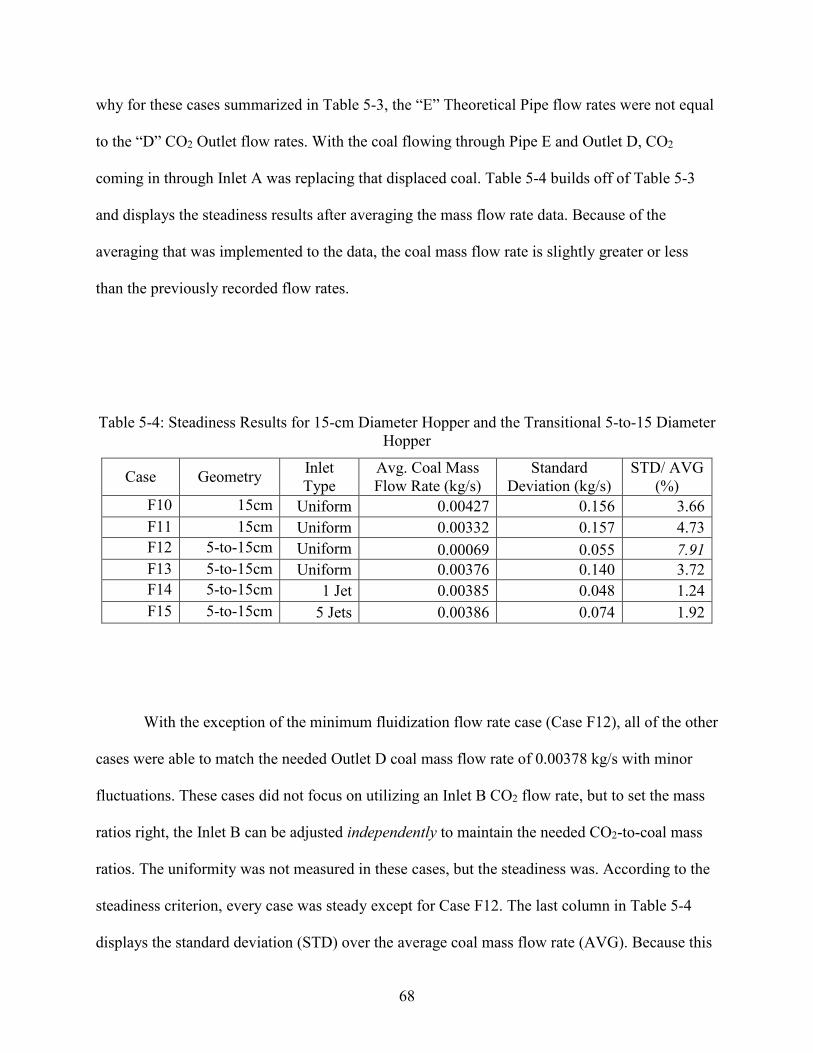
68

why for these cases summarized in Table 5-3, the “E” Theoretical Pipe flow rates were not equal

to the “D” CO2 Outlet flow rates. With the coal flowing through Pipe E and Outlet D, CO2

coming in through Inlet A was replacing that displaced coal. Table 5-4 builds off of Table 5-3

and displays the steadiness results after averaging the mass flow rate data. Because of the

averaging that was implemented to the data, the coal mass flow rate is slightly greater or less

than the previously recorded flow rates.

Table 5-4: Steadiness Results for 15-cm Diameter Hopper and the Transitional 5-to-15 Diameter Hopper

Case Geometry Inlet Type

Avg. Coal Mass Flow Rate (kg/s)

Standard Deviation (kg/s)

STD/ AVG (%)

F10 15cm Uniform 0.00427 0.156 3.66 F11 15cm Uniform 0.00332 0.157 4.73 F12 5-to-15cm Uniform 0.00069 0.055 7.91 F13 5-to-15cm Uniform 0.00376 0.140 3.72 F14 5-to-15cm 1 Jet 0.00385 0.048 1.24 F15 5-to-15cm 5 Jets 0.00386 0.074 1.92

With the exception of the minimum fluidization flow rate case (Case F12), all of the other

cases were able to match the needed Outlet D coal mass flow rate of 0.00378 kg/s with minor

fluctuations. These cases did not focus on utilizing an Inlet B CO2 flow rate, but to set the mass

ratios right, the Inlet B can be adjusted independently to maintain the needed CO2-to-coal mass

ratios. The uniformity was not measured in these cases, but the steadiness was. According to the

steadiness criterion, every case was steady except for Case F12. The last column in Table 5-4

displays the standard deviation (STD) over the average coal mass flow rate (AVG). Because this

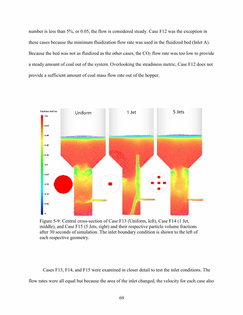
69

number is less than 5%, or 0.05, the flow is considered steady. Case F12 was the exception in

these cases because the minimum fluidization flow rate was used in the fluidized bed (Inlet A).

Because the bed was not as fluidized as the other cases, the CO2 flow rate was too low to provide

a steady amount of coal out of the system. Overlooking the steadiness metric, Case F12 does not

provide a sufficient amount of coal mass flow rate out of the hopper.

Cases F13, F14, and F15 were examined in closer detail to test the inlet conditions. The

flow rates were all equal but because the area of the inlet changed, the velocity for each case also

Figure 5-9: Central cross-section of Case F13 (Uniform, left), Case F14 (1 Jet, middle), and Case F15 (5 Jets, right) and their respective particle volume fractions after 30 seconds of simulation. The inlet boundary condition is shown to the left of each respective geometry.

70

changed. The three geometries and boundary condition for Inlet A are shown in Figure 5-9. The

fluidization of the uniform inlet was similar to that of the 5 Jets case where the fluidization of the

particles seemed to abruptly end once the hopper started expanding from the 5 to the 15 cm. As

previously seen in Figure 5-6 for the centrally concentrated inlet, the CO2 has a greater velocity

and tunnels through the packed bed. The uniform or 5-Jet inlet condition is more appropriate

because it provides a uniform fluidization of the bed. When compared with the larger 15-cm

diameter bed geometry (Case F10 and Case F11), the transitional 5-to-15-cm diameter bed

geometry (Cases F12, F13, F14, and F15) exhibited better fluidization of the entire bed with

exiting coal flow rates more accurate and precise.

71

6 PIPING SYSTEM

This chapter summarizes the tests performed to analyze the layout and roping of particles

moving through long horizontal pipe sections as well as various bend radii. The final piping

geometry is unknown because relative positions of the actual feed hopper and reactor have not

been determined. Therefore, an analysis of individual piping components was completed to give

insight into the flow behavior of components that could be used in various configurations.

6.1 Horizontal Pipe Behavior

A key feature of the feed system is that it delivers coal particles to the reactor in a steady

and uniform manner. For dense-phase flow in a horizontal pipe, the coal moves as a group of

particles. This occurs when the gas velocity is below the saltation velocity. If the velocity is

greater than the saltation velocity, the flow will be a dilute phase flow. The saltation velocity can

be thought of as the minimum velocity of the gas required to move all the particles in a

horizontal pipe [14]. This does not mean all the particles are picked up, suspended, and move in

a uniform manner, but it does ensure that the particles do move down the pipe.

Case P1 was run with a given coal mass flow rate (0.00379 kg/s) and CO2 (0.000379

kg/s) coming down the vertical portion of the geometry as seen in Figure 6-1. This geometry

represents the portion of the feed system after the fluidized bed (hopper) (see Pipe E, Figure 5-1).

Once the coal and CO2 reached the horizontal portion of the system, a horizontal flow of CO2

72

(0.003411 kg/s) conveyed the particles to the end of the system. Adding up the two CO2 mass

flow rates equaled the coal mass flow rate of 0.00379 kg/s and this led to a 1-to-1 ratio of CO2-

to-coal in the horizontal pipe. This CO2 flow rate converts to a velocity of 3.39 m/s and is an

order of magnitude greater than the pickup velocity (0.173 m/s, see Equation 2-10). This is

similar to the gravity-fed system simulated earlier, but instead of allowing particles to drop from

the standpipe, the particles are given a specific mass flow rate ensuring a proper coal mass flow

rate and loading ratio of CO2-to-coal mass flow rates. In the literature, the solids loading ratio

refers to solids flow rate over the fluid flow rate. From here onward, the “gas loading ratio”

refers to the fluid flow rate over the solids flow rate, or the CO2-to-coal mass flow rate ratio.

Simulations were conducted for a flowing period of 15 seconds. Initially, there were no

coal particles in the system. After the coal was introduced at the top of the vertical standpipe, the

coal reached the end of the 60.96-cm (24-in) length of pipe in about 0.25 seconds. As seen in

Figure 6-2, after about 30-cm of transport in the horizontal pipe, the particles started to drop out

and form a stratified flow on the bottom of the pipe. There are also dune formations towards the

end of the pipe above the stratified layer. Visually, these look like waves on the ocean moving

Figure 6-1: Geometry of the 60.96-cm long system.

73

through the pipe. Dune formation is undesired because this can lead to unsteady flows where the

coal builds up and suddenly exits the pipe leading to clumps and then gaps in the flow.

Based on the high definition of the sampling rate of the coal and CO2 exiting the pipe, the

coal mass flow rate never exceeded 0.009 kg/s and never was below 0.00175 kg/s. At this

sampling rate, looking at the times 5-15 seconds, there were 53,049 data points of coal mass flow

rate, the average flow rate was 0.003789 kg/s with a standard deviation of 0.0006849 kg/s. As

seen in Table 6-1, when averaged-down, there were 106 data points over the span of 10 seconds,

the average flow rate was 0.003790 kg/s with a standard deviation of 0.00003694 kg/s. The

standard deviation reduced by an order of magnitude to less than one percent of the average coal

flow rate. This was a steady flow rate of coal based on the ratio of the standard deviation over the

average coal flow rate being less than five percent.

Figure 6-2: Case P1 snapshot of the 60.96-cm long pipe mid-simulation. The bottom zoomed out image depicts the layout of particles as the flow continues towards the exit. The top zoomed- in portion portrays the last 10-cm of the pipe and formation of two dunes.

74

Table 6-1: Comparison of the Original Data and Averaged-Down Data for the Coal Mass Flow Rate for the 60.96-cm Horizontal Pipe

Variable Original Data

Averaged-Down

Percent (%) of Averaged-Down/Original

Data Points 53049 106 0.1998 Mass Flow Rate (kg/s) 3.789E-3 3.790E-3 100.01

Standard Deviation (kg/s) 6.849E-4 3.694E-5 5.394 STD/Mass Flow Rate 0.1807 0.009747 5.393

As a result of averaging down, the average coal mass flow rate remained the same at

0.00379 kg/s, but the standard deviation of the coal mass flow decreased by 94.6% and the ratio

of the standard deviation of the coal mass flow rate over the average coal mass flow rate also

decreased by 94.6%. Because the ratio of the standard deviation over the average flow rate was

equal to 0.009747, or 0.975%, this signified that by averaging down the data to a more realistic

sampling rate of 1 or 2 samples per second, the flow of coal was steadier than previously

observed. In practical terms, the realistic sampling rate was a better representation of how the

burner would respond to variations in coal flow. Flow fluctuations occurring at tenths or

hundredths of seconds would not be significant to burner operation. Conversely, fluctuations

occurring at scales of a half-second or one second would impact burner performance. Thus the

reduced sampling rate was a more practical measure of steadiness for this feed system.

Similar to the 60.96-cm long pipe, a 121.92-cm (48-in) long pipe, Case P2, was simulated

and Figure 6-3 shows particle layout starting at the same location as in the 60.96-cm long pipe

which occurred 30 cm down the pipe. By the end of the pipe, the stratified flow was more

pronounced and visible in the post-processing images. There was dune-flow and few particles

were suspended when exiting the pipe. The biggest change in the 121.92-cm long pipe when

comparing it to the 60.96-cm long pipe is that the standard deviation (0.001120 kg/s) was 29.6%

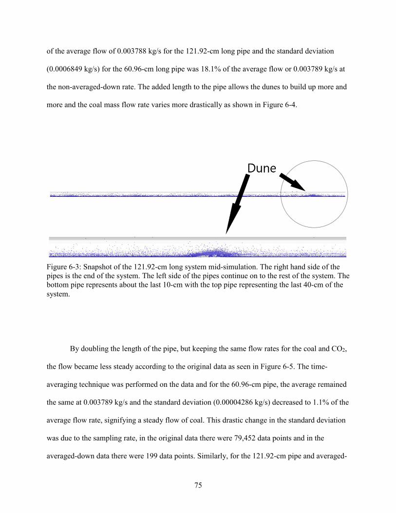
75

of the average flow of 0.003788 kg/s for the 121.92-cm long pipe and the standard deviation

(0.0006849 kg/s) for the 60.96-cm long pipe was 18.1% of the average flow or 0.003789 kg/s at

the non-averaged-down rate. The added length to the pipe allows the dunes to build up more and

more and the coal mass flow rate varies more drastically as shown in Figure 6-4.

By doubling the length of the pipe, but keeping the same flow rates for the coal and CO2,

the flow became less steady according to the original data as seen in Figure 6-5. The time-

averaging technique was performed on the data and for the 60.96-cm pipe, the average remained

the same at 0.003789 kg/s and the standard deviation (0.00004286 kg/s) decreased to 1.1% of the

average flow rate, signifying a steady flow of coal. This drastic change in the standard deviation

was due to the sampling rate, in the original data there were 79,452 data points and in the

averaged-down data there were 199 data points. Similarly, for the 121.92-cm pipe and averaged-

Figure 6-3: Snapshot of the 121.92-cm long system mid-simulation. The right hand side of the pipes is the end of the system. The left side of the pipes continue on to the rest of the system. The bottom pipe represents about the last 10-cm with the top pipe representing the last 40-cm of the system.

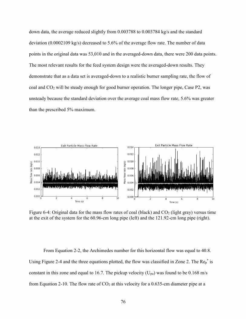
76

down data, the average reduced slightly from 0.003788 to 0.003784 kg/s and the standard

deviation (0.0002109 kg/s) decreased to 5.6% of the average flow rate. The number of data

points in the original data was 53,010 and in the averaged-down data, there were 200 data points.

The most relevant results for the feed system design were the averaged-down results. They

demonstrate that as a data set is averaged-down to a realistic burner sampling rate, the flow of

coal and CO2 will be steady enough for good burner operation. The longer pipe, Case P2, was

unsteady because the standard deviation over the average coal mass flow rate, 5.6% was greater

than the prescribed 5% maximum.

From Equation 2-2, the Archimedes number for this horizontal flow was equal to 40.8.

Using Figure 2-4 and the three equations plotted, the flow was classified in Zone 2. The Rep* is

constant in this zone and equal to 16.7. The pickup velocity (Upu) was found to be 0.168 m/s

from Equation 2-10. The flow rate of CO2 at this velocity for a 0.635-cm diameter pipe at a

Figure 6-4: Original data for the mass flow rates of coal (black) and CO2 (light gray) versus time at the exit of the system for the 60.96-cm long pipe (left) and the 121.92-cm long pipe (right).

77

pressure of 2.068 MPa was equal to 1.938 x 10-4 kg/s. If the CO2 mass flow rate was lower than

this, then the particles would not be picked up. They would be transported, but as a stratified

layer of particles moving along the bottom of the pipe.

To increase the steadiness of the flow, or decrease the fluctuation in the coal mass flow

rate a higher CO2 mass flow rate was needed. The ratio of 1-to-1 is on the low end and likely will

be higher in the real system depending on the burner operation. There will be enough CO2 to

increase the ratio close to 2-to-1, which should decrease the standard deviation in the coal mass

flow rate. This was accomplished by increasing the CO2 flow through the horizontal inlet making

the ratio 2-to-1. For Case P3, the exiting coal mass flow rate was maintained at 0.003790 kg/s

and the standard deviation of coal mass flow rate was decreased from 0.001126 kg/s to 0.000963

kg/s. The ratio of the standard deviation over the average flow rate reduced from 0.297 to 0.254

for the original data. For the averaged-down data, the ratio of the standard deviation over the

Figure 6-5: Averaged-down data shown to compare with the data recorded in Figure 6-4) The 60.96-cm horizontal pipe test is on the left and the 121.92-cm horizontal pipe is on the right.

78

average coal mass flow rate reduced from 5.6% to 2.6%, signifying a steady flow because of the

additional CO2. It is evident that increasing the flow rate of the CO2 increases the steadiness of

the coal mass flow. By increasing the CO2 mass flow rate, the steadiness of the flow increased

and the layout location shifted down to about 50 cm from where the coal is introduced to the

horizontal pipe.

From looking at the 60.96-cm (Case P1) and 121.92-cm horizontal pipes (Case P2 and

P3), it is evident that the 1-to-1 flow will have particle layout on the bottom of the pipe. To

achieve a uniform flow, a faster flow rate of CO2 is needed. A 2-to-1 flow was tested and the

results were compared visually with the 121.92-cm long pipe as seen in Figure 6-6. It is clear

from the images that the 1-to-1 mass flow exhibits more layout than the 2-to-1 mass flow. The

particle volume fraction reached about 0.48 for the 1-to-1 flow and 0.18 for the 2-to-1 flow. In

later tests, flux planes were defined in small areas across the pipe to measure the coal mass flow

rate in each area (see Section 6.2.4 and Figure 6-18). Once measured, the percent flow rate in

each area was calculated and this was how flow uniformity was characterized.

Along with looking at the layout of the particles, the impact of particle radius was

evaluated. Initial simulations were run using a mono-sized distribution, or a constant particle size

diameter of 75 µm. To better reflect possible experiments and an operational environment, a log-

normal poly-disperse distribution typical of pulverized coal was chosen with particle diameters

ranging from 6.7 µm to 272.2 µm. This distribution can be seen in Figure 6-7. The distribution

had a Sauter Mean Diameter (SMD) of 28.2 µm and a Mass Mean Diameter (MMD) of 54.9 µm.

The table inside the figure represents bins where a specific amount of the mass fraction resides.

Therefore, the smaller particles, e.g. the 3.35 µm radius bin containing 0.025 of the mass

fraction, has more particles than the 136.1 µm radius bin also containing 0.025 of the mass

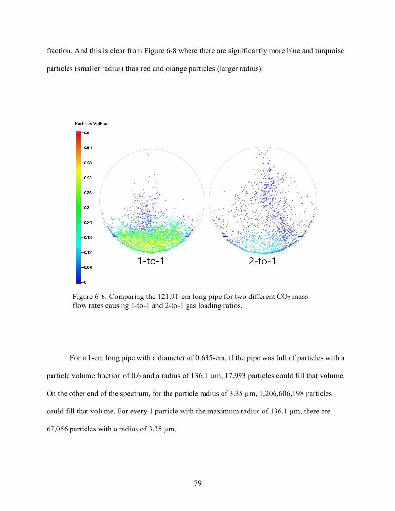
79

fraction. And this is clear from Figure 6-8 where there are significantly more blue and turquoise

particles (smaller radius) than red and orange particles (larger radius).

For a 1-cm long pipe with a diameter of 0.635-cm, if the pipe was full of particles with a

particle volume fraction of 0.6 and a radius of 136.1 µm, 17,993 particles could fill that volume.

On the other end of the spectrum, for the particle radius of 3.35 µm, 1,206,606,198 particles

could fill that volume. For every 1 particle with the maximum radius of 136.1 µm, there are

67,056 particles with a radius of 3.35 µm.

Figure 6-6: Comparing the 121.91-cm long pipe for two different CO2 mass flow rates causing 1-to-1 and 2-to-1 gas loading ratios.

80

From Case P3 that ran the 121.92-cm long pipe with a 2-to-1 ratio of CO2-to-coal, the

particle radius was tracked and a snapshot of the last 7.62-cm of pipe was taken. The view is

Figure 6-8: View of the particle radius looking down the end of pipe (last 7.62 cm) with the flow coming out of the page. Top, side, and bottom views are also shown with the flow direction indicated with arrows.

Figure 6-7: Particle size distribution for the coal used in most simulations.

81

looking into the exit of the pipe and the remaining 114 cm of pipe was removed from view (7.62-

cm showing). Because of this view, it combines 3D data all into a 2D view. Although it appears

there are a lot of particles distributed through the pipe, when looking at the top, side, and bottom

views it is clear that the majority of the particles are on the bottom of the pipe. There is a clear

stratified layer on the bottom of the pipe as well as particles forming dunes above the stratified

layer. The larger particles are gathering on the bottom of the pipe while the smaller particles are

still suspended by the end of the 122 cm.

For any length pipe longer than 30 cm and for a 1-to-1 gas loading ratio where both the

coal and CO2 mass flow rates are equal to 0.00378 kg/s, the particles will start to lay out on the

bottom of the pipe. If particle layout is to be avoided a higher CO2 mass flow rate is needed or

the horizontal portion of the pipe cannot be longer than 30 cm. When comparing the pressure

drops per unit length, for the 61-cm long pipe, the 1-to-1 mass ratio flow had a pressure drop of

1902 Pa/m from the beginning of where the coal particles drop into the horizontal section to the

exit of the system. For the 122-cm long pipe and a 1-to-1 mass ratio, the pressure drop was 1382

Pa/m. For the 2-to-1 mass ratio for the 122-cm long pipe, the pressure drop was 3556 Pa/m.

6.2 Bend Radius Impact

After learning about layout, tests were performed to determine the effect the bend radius

had on pressure drop, flow steadiness, and flow uniformity. The coal-CO2 flow is fed to a burner

at the top of the vertical reactor along with oxygen (O2) and more dilution CO2. This requires the

feed system to move the coal in multiple directions. The coal is expected to exit the bottom of

the hopper and then will need to be fed at the top of the vertical reactor. Multiple turns and

directions changes are likely to connect the outlet of the hopper to the inlet of the burner. Three

82

different bends were tested to determine the behavior of the coal particles flowing around the

bends: a horizontal-to-horizontal bend, a horizontal-to-upward vertical bend, and a horizontal-to-

downward vertical bend. With each of these three bend directions, two CO2 mass flow rates were

tested (1-to-1 flow ratio and 2-to-1 flow ratio) and two bend radii were tested for the 0.635-cm

diameter pipe: a 90° bend (bend radius equal to 0.3175-cm or 0.125-in) and a larger bend (bend

radius equal to 60.96-cm or 24-in). Theses six bends are shown in Figure 6-9.

As a particle-laden flow encounters a pipe bend, roping will occur and the particles will

group together on the far side of the pipe as seen in Figure 6-10. Even after a long ways

downstream from a bend, particles tend to stay grouped on the far side of the pipe. This comes

back to Newton’s First Law: an object in motion wants to stay in motion. The particles want to

Figure 6-9: Schematic showing orientation of the three sharp 90° bends (left) and the three larger bend radii (right) mapped on a Cartesian coordinate system.

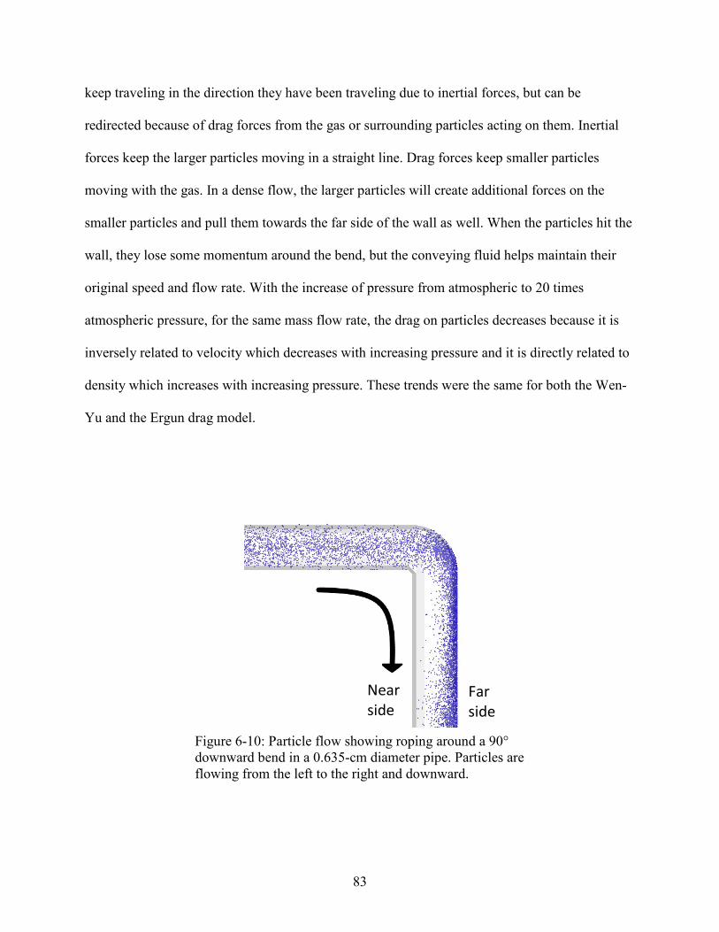
83

keep traveling in the direction they have been traveling due to inertial forces, but can be

redirected because of drag forces from the gas or surrounding particles acting on them. Inertial

forces keep the larger particles moving in a straight line. Drag forces keep smaller particles

moving with the gas. In a dense flow, the larger particles will create additional forces on the

smaller particles and pull them towards the far side of the wall as well. When the particles hit the

wall, they lose some momentum around the bend, but the conveying fluid helps maintain their

original speed and flow rate. With the increase of pressure from atmospheric to 20 times

atmospheric pressure, for the same mass flow rate, the drag on particles decreases because it is

inversely related to velocity which decreases with increasing pressure and it is directly related to

density which increases with increasing pressure. These trends were the same for both the Wen-

Yu and the Ergun drag model.

Figure 6-10: Particle flow showing roping around a 90° downward bend in a 0.635-cm diameter pipe. Particles are flowing from the left to the right and downward.

Near side

Far side

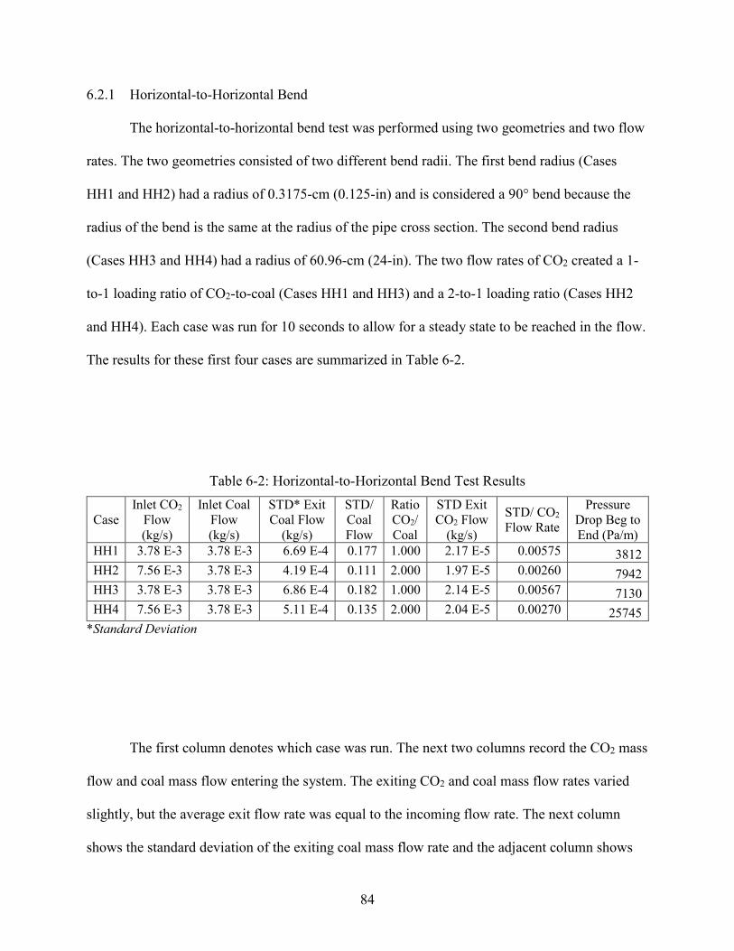
84

6.2.1 Horizontal-to-Horizontal Bend

The horizontal-to-horizontal bend test was performed using two geometries and two flow

rates. The two geometries consisted of two different bend radii. The first bend radius (Cases

HH1 and HH2) had a radius of 0.3175-cm (0.125-in) and is considered a 90° bend because the

radius of the bend is the same at the radius of the pipe cross section. The second bend radius

(Cases HH3 and HH4) had a radius of 60.96-cm (24-in). The two flow rates of CO2 created a 1-

to-1 loading ratio of CO2-to-coal (Cases HH1 and HH3) and a 2-to-1 loading ratio (Cases HH2

and HH4). Each case was run for 10 seconds to allow for a steady state to be reached in the flow.

The results for these first four cases are summarized in Table 6-2.

Table 6-2: Horizontal-to-Horizontal Bend Test Results

Case Inlet CO2

Flow (kg/s)

Inlet Coal Flow (kg/s)

STD* Exit Coal Flow

(kg/s)

STD/ Coal Flow

Ratio CO2/ Coal

STD Exit CO2 Flow

(kg/s)

STD/ CO2 Flow Rate

Pressure Drop Beg to End (Pa/m)

HH1 3.78 E-3 3.78 E-3 6.69 E-4 0.177 1.000 2.17 E-5 0.00575 3812 HH2 7.56 E-3 3.78 E-3 4.19 E-4 0.111 2.000 1.97 E-5 0.00260 7942 HH3 3.78 E-3 3.78 E-3 6.86 E-4 0.182 1.000 2.14 E-5 0.00567 7130 HH4 7.56 E-3 3.78 E-3 5.11 E-4 0.135 2.000 2.04 E-5 0.00270 25745

*Standard Deviation

The first column denotes which case was run. The next two columns record the CO2 mass

flow and coal mass flow entering the system. The exiting CO2 and coal mass flow rates varied

slightly, but the average exit flow rate was equal to the incoming flow rate. The next column

shows the standard deviation of the exiting coal mass flow rate and the adjacent column shows

85

the ratio of the standard deviation over the average exiting coal mass flow rate. The next column

records the mass flow ratios of CO2-to-coal. The next two columns show the standard deviation

of the exiting CO2 mass flow rate and the ratio of the standard deviation over the average exiting

CO2 mass flow rate. The last column records the pressure drop per meter in the system.

A key difference in the two geometries is the distance the particles traveled. For each

case the particles traveled 15.24 cm (6-in) before and after the bend. The difference is the 90°

bend radius was only 0.3175 cm making the extra distance equal to 0.499 cm while the larger

bend (60.96 cm) added an extra 95.756 cm the coal particles had to travel a distance of (2𝜋𝜋𝜋𝜋/4)

around the bend. This extra distance for Cases HH3 and HH4 accounts for the larger pressure

drop in the system. Surprisingly, the extra distance did not increase the standard deviation of the

coal mass flow rate by much. The increase of the standard deviation over the coal mass flow rate

ratio was less than 1% comparing Cases HH1 and HH3 (lower CO2 mass flow rate) and the

increase was about 2.5% from Case HH2 to Case HH4 (higher CO2 mass flow rate).

Looking at Case HH1, the particles start to layout before they reach the pipe bend. When

the particles go around the bend and because of the nature of the bend as seen in Figure 6-11, the

particles swirl around and make their way up the side and up to the top of the pipe. From the

front view, there is a clear gap where very few particles are visible on the bottom of the pipe

right after the bend in the pipe. For Case HH2, where the CO2 mass flow rate was doubled

maintaining the same amount of coal flow, the same swirling effect occurred, but because of the

doubled CO2 mass flow rate, the particles were moving faster, there was less layout, and thus

less particles were swirled around the pipe after the bend.

Swirling will occur in a sharp 90° bend whenever the particles are grouped together

before the bend. For Case HH2, the particles did not lay out and group together as much as Case

86

HH1. Therefore, there was less swirling for Case HH2. For both cases, the particles swirled up to

the top of the pipe and stayed suspended with little drop out until the end of the pipe. With a

longer pipe after the bend, the particles would eventually continue to lay out with the smaller

(less massive) particles remaining suspended in the CO2 flow.

For Cases HH3 and HH4 (larger bend radius), the roping was more gradual and the

swirling effect was minimal. This was due to the bend radius. The bend was more gradual and

the coal particles grouped together on the far side of the pipe. With the 2-to-1 flow rate for Test

HH4, the build-up of particles decreased slightly compared to Case HH3. Because it was a faster

flow rate in Case HH4, the particles can be seen in Figure 6-12 roping higher up the far side of

the pipe. For Case HH3, there were particle volume fractions close to 0.5 and for Case HH4, the

highest the particle volume fraction reached 0.3 to 0.35.

Figure 6-11: Particles of Case HH1 mid-simulation with the front view particles flowing from left to right (top) and back view particles flowing from right to left (bottom) shown of the horizontal 90° bend.

87

If particles are roped on the top side or laid out on the bottom side for a horizontal-to-

horizontal bend, the particles will swirl around the bend if the bend has a small bend radius. To

reduce swirling, a larger bend radius should be implemented, but this will increase roping

effects.

6.2.2 Horizontal-to-Upward Vertical Bend

Of the three different bends tested, the horizontal-to-upward vertical bend was shown to

be the least steady. Table 6-3 shows that all of the averages were consistent, but the fluctuations,

or standard deviations were the greatest in this orientation. Similar to the horizontal-to-horizontal

Figure 6-12: Snapshot of the particles at the end of the bend after ten seconds of simulation of Case HH3 (left) and Case HH4 (right). Left of each gray circle is where the bend ends. This view is looking straight into the exit of the pipe with particles and gas coming out of the page.

88

bends, the flow travelled horizontally for a distance and then went through a 90° bend (smaller or

larger radius) and then travelled upwards in the vertical direction. These tests will be referred to

as Cases HU5, HU6, HU7, and HU8. Cases HU5 and HU6 used the small bend radius of 0.3175

cm (0.125-in), or a sharp 90° bend, and Cases HU7 and HU8 used the larger bend radius of

60.96 cm (24-in). Cases HU5 and HU7 used a 1-to-1 loading ratio of CO2-to-coal and Cases

HU6 and HU8 used a 2-to-1 loading ratio of CO2-to-coal.

As stated in the previous section, the first column denotes which case was run. The next

two columns record the CO2 mass flow and coal mass flow entering the system. The exiting CO2

and coal mass flow rates varied slightly, but the average exit flow rate was equal to the incoming

flow rate. The next column shows the standard deviation of the exiting coal mass flow rate and

the adjacent column shows the ratio of the standard deviation over the average exiting coal mass

flow rate. The next column records the mass flow ratios of CO2-to-coal. The next two columns

show the standard deviation of the exiting CO2 mass flow rate and the ratio of the standard

deviation over the average exiting CO2 mass flow rate. The last column records the pressure drop

per meter in the system.

Table 6-3: Horizontal-to-Upward Vertical Bend Test Results

Case Inlet CO2

Flow (kg/s)


STD* Coal Flow

(kg/s)

STD/ Coal Flow

Ratio CO2/ Coal

STD CO2 Flow (kg/s)

STD/ CO2 Flow Rate

Pressure Drop Beg to End (Pa/m)

HU5 3.78 E-3 3.78 E-3 7.47 E-4 0.198 1.000 2.35E-5 0.00621 3177 HU6 7.56 E-3 3.78 E-3 4.55 E-4 0.120 2.000 1.95E-5 0.00258 4765 HU7 3.78 E-3 3.78 E-3 7.85 E-4 0.208 1.000 2.48E-5 0.00655 7922 HU8 7.56 E-3 3.78 E-3 6.90 E-4 0.183 2.000 2.46E-5 0.00326 22973

*STD – standard deviation without down averaging

89

The biggest difference for these set of tests relative to the horizontal-to-horizontal tests

was that the flow was directly opposite of gravity after the bend. For these tests and all the bend

tests, the force of gravity was in the “-Z” direction. As the particles and gas entered the pipe,

they started to layout and group together on the bottom of the pipe. Once the particles went

through the bend, the majority remained on the far side until the exit. There was no swirling in

this system and by the end of the pipe some particles did redistribute themselves. The

gravitational forces added drag on the particles that the flow had to overcome. The roping effects

were observed at the end of the pipe. The particle volume fraction image can be seen in Figure

6-13. The two large circles in the figure are: 1) Looking down the beginning of the pipe prior to

the bend, and 2) Looking down the end of the pipe downstream after the bend. The pipe is cut at

the 7.62-cm (3-in) mark so half of the pipe is shown for each image in their corresponding

direction to better show the distribution of the particles.

When comparing the end views in Figure 6-14 of all the vertical bend tests, they all look

similar to each other. For the larger bend radius (Cases HU7 and HU8), there is slight

improvement when looking at the particle volume fraction and the distribution of the particles in

the pipe. For the same 1-to-1 flow rates, Case HU7 (large radius) appears to be better than Case

HU5 (small radius). The particles are more disperse, there are lower particle volume fractions,

and there is less roping. And similarly for the 2-to-1 flow rates, Case HU8 (large radius) has a

slightly better distribution of particles than Case HU6 (small radius) when looking at the right

wall (far side) where the roping occurred.

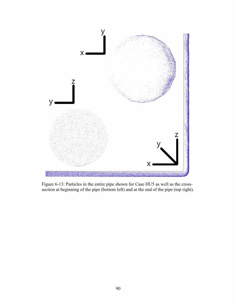
90

Figure 6-13: Particles in the entire pipe shown for Case HU5 as well as the cross-section at beginning of the pipe (bottom left) and at the end of the pipe (top right).

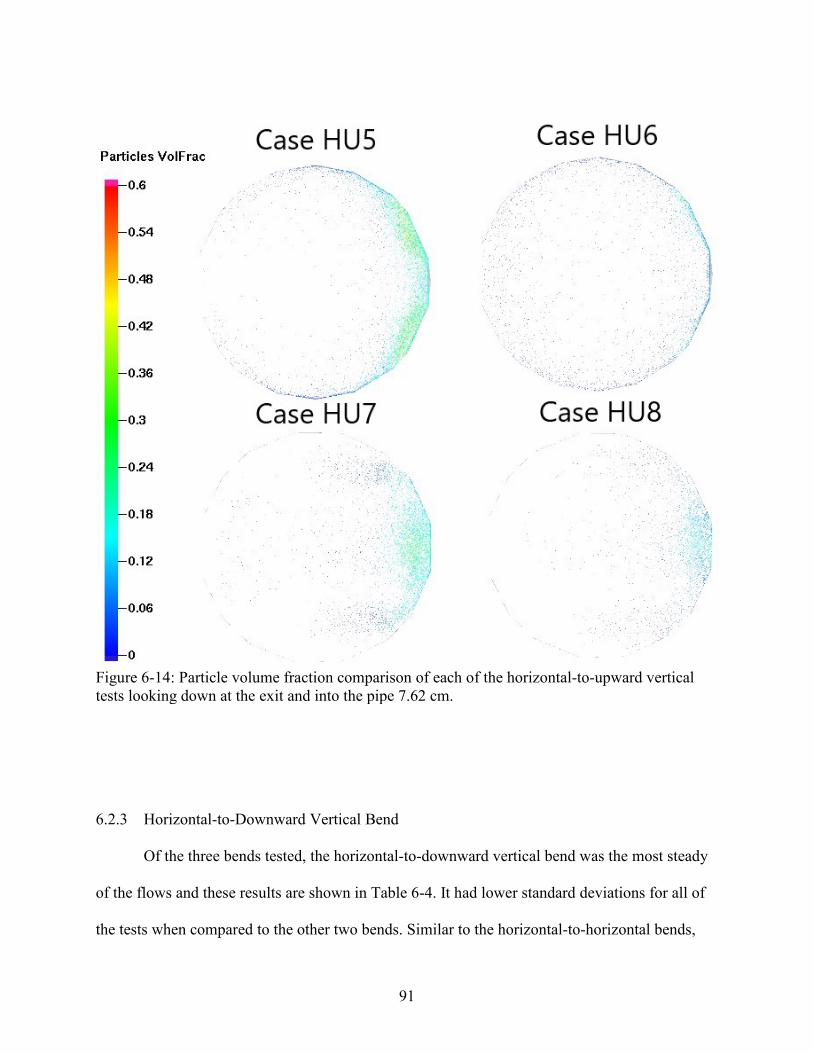
91

6.2.3 Horizontal-to-Downward Vertical Bend

Of the three bends tested, the horizontal-to-downward vertical bend was the most steady

of the flows and these results are shown in Table 6-4. It had lower standard deviations for all of

the tests when compared to the other two bends. Similar to the horizontal-to-horizontal bends,

Figure 6-14: Particle volume fraction comparison of each of the horizontal-to-upward vertical tests looking down at the exit and into the pipe 7.62 cm.

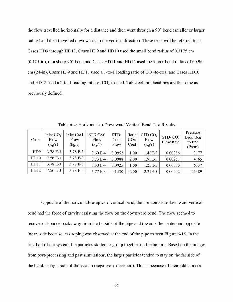
92

the flow travelled horizontally for a distance and then went through a 90° bend (smaller or larger

radius) and then travelled downwards in the vertical direction. These tests will be referred to as

Cases HD9 through HD12. Cases HD9 and HD10 used the small bend radius of 0.3175 cm

(0.125-in), or a sharp 90° bend and Cases HD11 and HD12 used the larger bend radius of 60.96

cm (24-in). Cases HD9 and HD11 used a 1-to-1 loading ratio of CO2-to-coal and Cases HD10

and HD12 used a 2-to-1 loading ratio of CO2-to-coal. Table column headings are the same as

previously defined.

Table 6-4: Horizontal-to-Downward Vertical Bend Test Results

Case Inlet CO2

Flow (kg/s)


STD Coal Flow (kg/s)

STD/ Coal Flow

Ratio CO2/ Coal

STD CO2 Flow (kg/s)

STD/ CO2 Flow Rate

Pressure Drop Beg

to End (Pa/m)

HD9 3.78 E-3 3.78 E-3 3.60 E-4 0.0952 1.00 1.46E-5 0.00386 3177 HD10 7.56 E-3 3.78 E-3 3.73 E-4 0.0988 2.00 1.95E-5 0.00257 4765 HD11 3.78 E-3 3.78 E-3 3.50 E-4 0.0925 1.00 1.25E-5 0.00330 6337 HD12 7.56 E-3 3.78 E-3 5.77 E-4 0.1530 2.00 2.21E-5 0.00292 21389

Opposite of the horizontal-to-upward vertical bend, the horizontal-to-downward vertical

bend had the force of gravity assisting the flow on the downward bend. The flow seemed to

recover or bounce back away from the far side of the pipe and towards the center and opposite

(near) side because less roping was observed at the end of the pipe as seen Figure 6-15. In the

first half of the system, the particles started to group together on the bottom. Based on the images

from post-processing and past simulations, the larger particles tended to stay on the far side of

the bend, or right side of the system (negative x-direction). This is because of their added mass

93

and inertial forces acting more on those particles. The images for the inlet and outlet views are

looking at 7.62 cm of the pipe, or about half of the corresponding horizontal (inlet) and vertical

(outlet) portions of the system.

Figure 6-15: Particle volume fraction of the entire pipe shown for Case HD9. The inlet (left) and outlet (right) cross-section are also shown to observe the roping effects of at the outlet. Gravity is in the negative Z-direction.

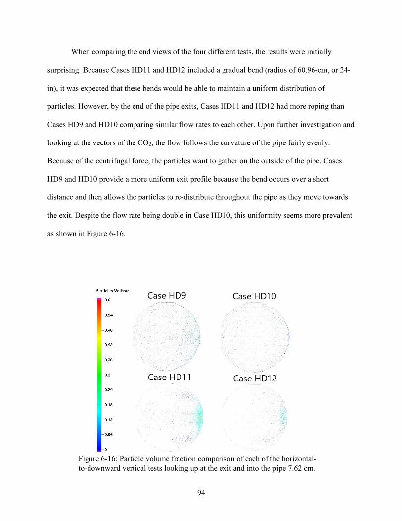
94

When comparing the end views of the four different tests, the results were initially

surprising. Because Cases HD11 and HD12 included a gradual bend (radius of 60.96-cm, or 24-

in), it was expected that these bends would be able to maintain a uniform distribution of

particles. However, by the end of the pipe exits, Cases HD11 and HD12 had more roping than

Cases HD9 and HD10 comparing similar flow rates to each other. Upon further investigation and

looking at the vectors of the CO2, the flow follows the curvature of the pipe fairly evenly.

Because of the centrifugal force, the particles want to gather on the outside of the pipe. Cases

HD9 and HD10 provide a more uniform exit profile because the bend occurs over a short

distance and then allows the particles to re-distribute throughout the pipe as they move towards

the exit. Despite the flow rate being double in Case HD10, this uniformity seems more prevalent

as shown in Figure 6-16.

Figure 6-16: Particle volume fraction comparison of each of the horizontal-to-downward vertical tests looking up at the exit and into the pipe 7.62 cm.

95

6.2.4 Very Large Bend Radius

Two additional cases were run increasing the bend radius from 60.96 cm (24-in) up to

182.88 cm (72-in). These tests were similar to the horizontal-to-downward vertical bend tests

because they had an initial horizontal section of 15.24 cm (6-in), the horizontal-to-downward

bend with the bend radius of 182.88 cm, and then a downward section of 15.24 cm to the exit.

These two tests will be referred to as Case HD13, which has a loading ratio of 1-to-1 and Case

HD14, which had a loading ratio of 2-to-1. When comparing these tests to the 60.96-cm bend

radius, the roping is more pronounced in the 182.88-cm bend radius. A side view of Cases

HD11, HD12, HD13, and HD14 are shown in Figure 6-17.

Figure 6-17: A side view of the particle volume fraction for Cases HD11-HD14. Cases HD11 and HD12 are the 60.96-cm bend radius and Cases HD13 and HD14 are the 182.88-cm bend radius.

96

Additional calculations were performed to determine the amount of particles in each

section of the exit. Flux planes were created in slices to measure the flow rate in each of the

planes and then divided by the total flow rate to find the ratio. Along with the qualitative

observations from viewing the particles in the post-processing of Barracuda, these planes

provided a quantitative value measuring the uniformity of the flow. The graphic with different

colors represent the different areas where the flow rate was measured. The right side (dark gray)

is where the roped flow would congregate and sometimes the majority of the flow would occur

in this area as seen Figure 6-18. The following numbers correspond to the various areas: Area 1 –

Light Gray, Area 2 – Orange, Area 3 – Purple, Area 4 – Green, Area 5, Blue, and Area 6 – Dark

Gray.

Figure 6-18: Cross-section view of the mesh for each pipe exit. Each color represents the area where a flux plane was placed to record results.

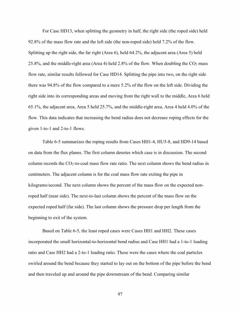
97

For Case HD13, when splitting the geometry in half, the right side (the roped side) held

92.8% of the mass flow rate and the left side (the non-roped side) held 7.2% of the flow.

Splitting up the right side, the far right (Area 6), held 64.2%, the adjacent area (Area 5) held

25.8%, and the middle-right area (Area 4) held 2.8% of the flow. When doubling the CO2 mass

flow rate, similar results followed for Case HD14. Splitting the pipe into two, on the right side

there was 94.8% of the flow compared to a mere 5.2% of the flow on the left side. Dividing the

right side into its corresponding areas and moving from the right wall to the middle, Area 6 held

65.1%, the adjacent area, Area 5 held 25.7%, and the middle-right area, Area 4 held 4.0% of the

flow. This data indicates that increasing the bend radius does not decrease roping effects for the

given 1-to-1 and 2-to-1 flows.

Table 6-5 summarizes the roping results from Cases HH1-4, HU5-8, and HD9-14 based

on data from the flux planes. The first column denotes which case is in discussion. The second

column records the CO2-to-coal mass flow rate ratio. The next column shows the bend radius in

centimeters. The adjacent column is for the coal mass flow rate exiting the pipe in

kilograms/second. The next column shows the percent of the mass flow on the expected non-

roped half (near side). The next-to-last column shows the percent of the mass flow on the

expected roped half (far side). The last column shows the pressure drop per length from the

beginning to exit of the system.

Based on Table 6-5, the least roped cases were Cases HH1 and HH2. These cases

incorporated the small horizontal-to-horizontal bend radius and Case HH1 had a 1-to-1 loading

ratio and Case HH2 had a 2-to-1 loading ratio. These were the cases where the coal particles

swirled around the bend because they started to lay out on the bottom of the pipe before the bend

and then traveled up and around the pipe downstream of the bend. Comparing similar

98

geometries, but with different flow rates (e.g., Cases HH1 and HH2 or Cases HH3 and HH4 or

Cases HU5 and HU6 and so on), the smaller CO2 flow rate always had the smaller pressure drop

which was expected. As the flow rate increased, the velocity increased, and the pressure drop

also increased.

Table 6-5: Roping Effects on All Bend Tests

Case CO2-to-

Coal Mass Ratio

Bend Radius (cm)

Coal Mass Flow Rate

(kg/s)

Percent of Flow on Non-Roped Half

Percent of Flow on

Roped Half

Pressure Drop/Length

(Pa/m) HH1 1 0.3175 3.7799 E-3 36.4 63.6 3812 HH2 2 0.3175 3.7800 E-3 36.9 63.1 7942 HH3 1 60.96 3.7805 E-3 9.1 90.9 7130 HH4 2 60.96 3.7801 E-3 5.2 94.8 25745 HU5 1 0.3175 3.7797 E-3 13.8 86.2 3177 HU6 2 0.3175 3.7800 E-3 32.8 67.2 4765 HU7 1 60.96 3.7789 E-3 2.7 97.3 7922 HU8 2 60.96 3.7798 E-3 3.7 96.3 22973 HD9 1 0.3175 3.7799 E-3 25.0 75.0 3177

HD10 2 0.3175 3.7800 E-3 31.9 68.1 4765 HD11 1 60.96 3.7803 E-3 3.5 96.5 6337 HD12 2 60.96 3.7799 E-3 3.7 96.3 21389 HD13 1 182.88 3.7792 E-3 4.9 95.1 8836 HD14 2 182.88 3.7795 E-3 3.3 96.7 28194

For each of the three different bends, the small bend radius (0.3175 cm) had the least

amount of roping by the end of the pipe. Consistently for the large radius (60.96 cm), 90% of the

flow rate occurred on the roped half of the pipe, or where the roping was expected to occur.

Contrary to initially thinking, the extra-large bend radius (182.88 cm) was similar to the large

99

radius and had over 90% of the flow in the roped half of the pipe. This makes sense that the

particles would agglomerate on the roped half because there are no forces or changes in the

geometry to make the particles come back to the other half of the pipe. The small bend radius

turns quickly and allows the particles to partially redistribute themselves throughout the rest of

the pipe before the exit of the system. Comparing the small bend radius turns with each of the

three orientations, the percent of flow in the roped area for the 2-to-1 flow was always smaller

than 1-to-1 flow.

Based on the distribution of the mass flow rate across the six areas of the pipe cross

section, the least amount of roping occurred with the small bend radius-tests. A case of interest is

Case HU7; while there is 90.9% on the roped half of the pipe, the majority of that flow occurs in

the middle of the pipe. Each bend geometry (e.g., horizontal-to-horizontal, horizontal-to-upward

vertical, and horizontal-to-downward vertical) was grouped together and the mass flow rate in

each area as shown in Figure 6-18 was plotted. These plots display the coal mass flow rate

through each of the perspective areas 1-6. Adding up each of these six flow rates equals the

average coal mass flow rate exiting the system.

The first plots are for the horizontal-to-horizontal bends (Cases HH1-4). Each case is

quite different than the other with the same geometry and or same flow rate as seen in Figure

6-19. These results were the most unpredictable and this was because of the swirling. The largest

flow rate was predicted to be in the far right area, Area 6 because of the roping phenomena. For

Case HH2, the largest flow rate was in the area adjacent to far area, Area 5 and for Case HH3,

the largest flow rate was in the middle-right area, Area 4. The figure breaks down the coal mass

flow rates in each area and plots them relative to each other. Every test had an average coal mass

flow rate of 0.00378 kg/s. For a uniform flow, the profile should appear as a parabola with little

100

flow in Areas 1 and 6 and the majority of the flow in Areas 2-5. There was significant roping for

Case HH3 and HH4 when compared Cases HH1 and HH2 because of the larger bend radius.

Looking at Area 6, Case HH1 had 25.3% of the mass flow rate in this area, Case HH2 had 15.4%

of the mass flow, Case HH3 had 10.5% of the mass flow rate, and Case HH4 had 45.9% of the

flow. For Case HH2, the largest flow rate was in Area 5, and the percentage was 26.0%. For

Case HH3 and in Area 4, this percentage was 42.6%

The next set of plots combine the horizontal-to-upward vertical bends (Cases HU5-8).

These cases were more consistent as seen in Figure 6-20 and they were more predictable than the

previous horizontal-to-horizontal tests. All the cases were similar to each other in that the mass

Figure 6-19: Coal mass flow rate plotted versus the vertical area section in the pipe for the horizontal-to-horizontal bend tests (Cases HH1-4).

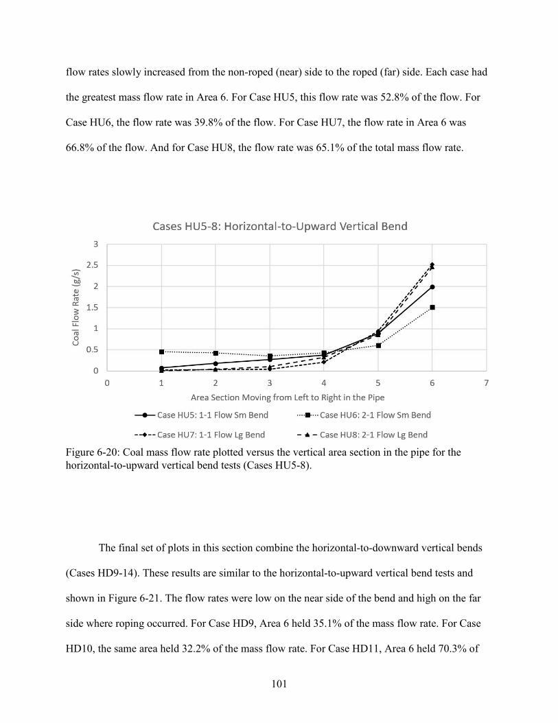
101

flow rates slowly increased from the non-roped (near) side to the roped (far) side. Each case had

the greatest mass flow rate in Area 6. For Case HU5, this flow rate was 52.8% of the flow. For

Case HU6, the flow rate was 39.8% of the flow. For Case HU7, the flow rate in Area 6 was

66.8% of the flow. And for Case HU8, the flow rate was 65.1% of the total mass flow rate.

The final set of plots in this section combine the horizontal-to-downward vertical bends

(Cases HD9-14). These results are similar to the horizontal-to-upward vertical bend tests and

shown in Figure 6-21. The flow rates were low on the near side of the bend and high on the far

side where roping occurred. For Case HD9, Area 6 held 35.1% of the mass flow rate. For Case

HD10, the same area held 32.2% of the mass flow rate. For Case HD11, Area 6 held 70.3% of

Figure 6-20: Coal mass flow rate plotted versus the vertical area section in the pipe for the horizontal-to-upward vertical bend tests (Cases HU5-8).

102

the mass flow rate, more than double the percent comparing to both Cases HD9 and HD10. For

Case HD12, the far side area held 66.2% of the mass flow rate. For Case HD13, the far side area

held 58.9% of the mass flow rate and for Case HD14, that same area held 59.5% of the mass

flow rate.

Based on the results from the bend radius tests, the bends should be a small radius and on

the order of the same size as the diameter of the pipe. Another consideration not evaluated in this

study is the impact of roping on pipe erosion. Erosion is a complex function of several flow

properties including particle impact angle, size and velocity. Generally, higher velocities lead to

Figure 6-21: Coal mass flow rate plotted versus the vertical area section in the pipe for the horizontal-to-downward vertical bend tests (Cases HD9-14).

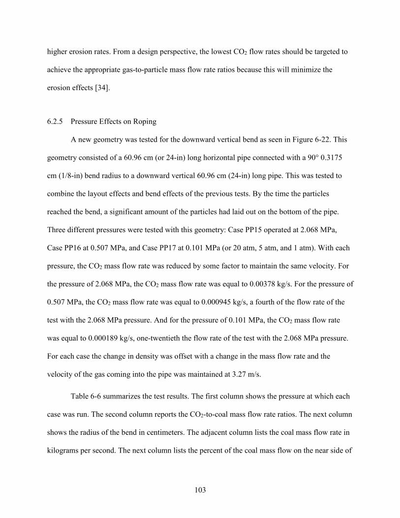
103

higher erosion rates. From a design perspective, the lowest CO2 flow rates should be targeted to

achieve the appropriate gas-to-particle mass flow rate ratios because this will minimize the

erosion effects [34].

6.2.5 Pressure Effects on Roping

A new geometry was tested for the downward vertical bend as seen in Figure 6-22. This

geometry consisted of a 60.96 cm (or 24-in) long horizontal pipe connected with a 90° 0.3175

cm (1/8-in) bend radius to a downward vertical 60.96 cm (24-in) long pipe. This was tested to

combine the layout effects and bend effects of the previous tests. By the time the particles

reached the bend, a significant amount of the particles had laid out on the bottom of the pipe.

Three different pressures were tested with this geometry: Case PP15 operated at 2.068 MPa,

Case PP16 at 0.507 MPa, and Case PP17 at 0.101 MPa (or 20 atm, 5 atm, and 1 atm). With each

pressure, the CO2 mass flow rate was reduced by some factor to maintain the same velocity. For

the pressure of 2.068 MPa, the CO2 mass flow rate was equal to 0.00378 kg/s. For the pressure of

0.507 MPa, the CO2 mass flow rate was equal to 0.000945 kg/s, a fourth of the flow rate of the

test with the 2.068 MPa pressure. And for the pressure of 0.101 MPa, the CO2 mass flow rate

was equal to 0.000189 kg/s, one-twentieth the flow rate of the test with the 2.068 MPa pressure.

For each case the change in density was offset with a change in the mass flow rate and the

velocity of the gas coming into the pipe was maintained at 3.27 m/s.

Table 6-6 summarizes the test results. The first column shows the pressure at which each

case was run. The second column reports the CO2-to-coal mass flow rate ratios. The next column

shows the radius of the bend in centimeters. The adjacent column lists the coal mass flow rate in

kilograms per second. The next column lists the percent of the coal mass flow on the near side of

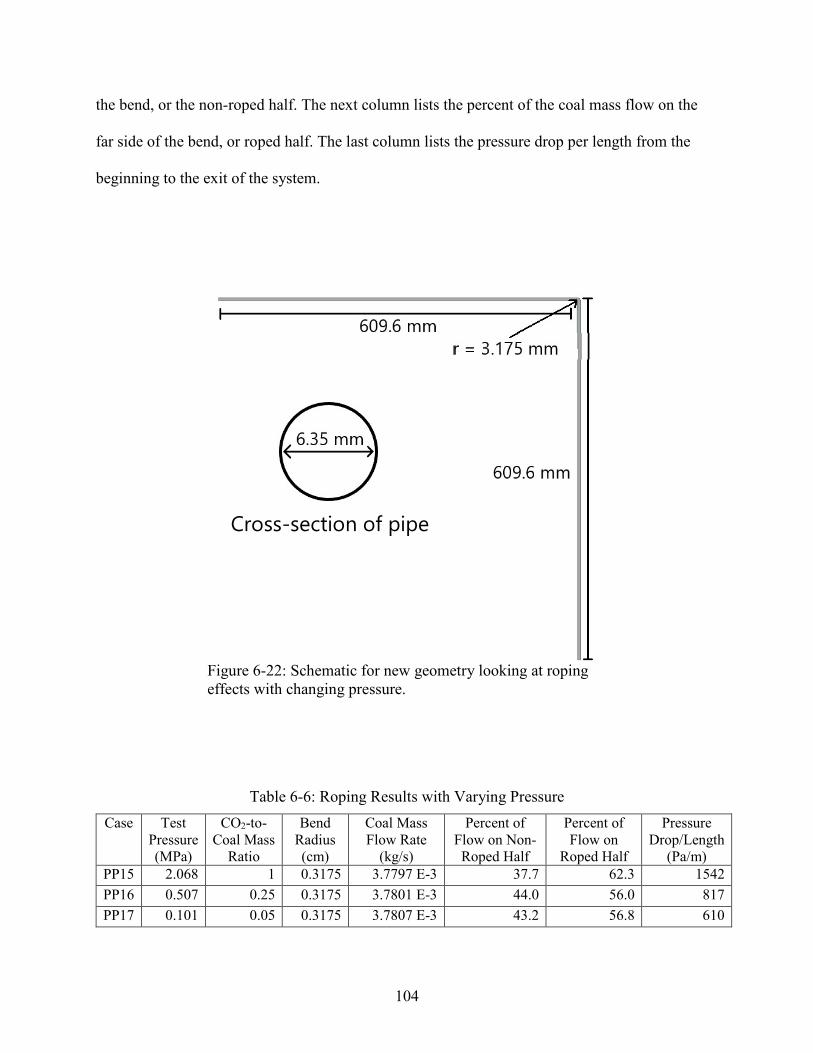
104

the bend, or the non-roped half. The next column lists the percent of the coal mass flow on the

far side of the bend, or roped half. The last column lists the pressure drop per length from the

beginning to the exit of the system.

Table 6-6: Roping Results with Varying Pressure Case Test

Pressure (MPa)

CO2-to-Coal Mass

Ratio

Bend Radius (cm)

Coal Mass Flow Rate

(kg/s)

Percent of Flow on Non-Roped Half

Percent of Flow on

Roped Half

Pressure Drop/Length

(Pa/m) PP15 2.068 1 0.3175 3.7797 E-3 37.7 62.3 1542 PP16 0.507 0.25 0.3175 3.7801 E-3 44.0 56.0 817 PP17 0.101 0.05 0.3175 3.7807 E-3 43.2 56.8 610

Figure 6-22: Schematic for new geometry looking at roping effects with changing pressure.

Cross-section of pipe

105

Based on the learnings from the previous section, the roping should have been minimal

because the bend was a sharp 90° bend and there was an extra 45.72 cm of pipe for the particles

to redistribute throughout the pipe. As seen previously in Table 6-5 and comparing results to

Table 6-6, the Case PP15 (2.068 MPa) results were similar to Cases HD9 and HD10 based on the

percent of the mass flow on the roped and non-roped halves, with Case PP16 (0.507 MPa) and

Case PP17 (0.101 MPa) having even lower percentages and closer to a 50-50 flow where half of

the flow was on the left side and the other half of the flow was on the right side. With the extra

length of the pipe the particles seemed to move towards the middle rather than the wall of the

pipe and a parabolic mass flow rate profile started to emerge as seen in Figure 6-23. When

comparing the different pressure (PP) tests to one another, Case PP16 had slightly higher

percentages of the flow rate on the roped side of the pipe. When comparing Figure 6-21 with

Figure 6-23, it is clear that the added length of pipe makes a difference in the distribution of the

coal throughout the pipe for all pressures. The other contribution to this behavior was the added

length of pipe at the beginning which caused the majority of the particles to lay out, or group

together on the bottom of the pipe prior to encountering the bend.

For the design of the piping system, the last bend to turn in the downward vertical

direction should be a sharp turn (bend radius of 0.3175-cm) and then have a sufficiently long

vertical section (>60-cm) to allow the particles to re-distribute themselves throughout the pipe.

The number of bends in the design should be minimized to reduce the effects of roping, but with

straight pipe-run effects, particles will lay out before and after the bends. With layout, swirling

effects will be present in horizontal-to-horizontal bends and the bend radius should be increased

to reduce these effects. Significant particle roping is likely to occur for all bend radii. Therefore,

it is unlikely that a uniform particle flow can be delivered to the burner. This may not be

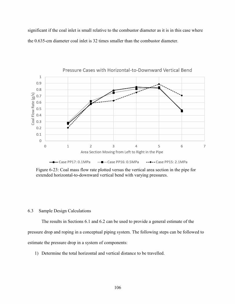
106

significant if the coal inlet is small relative to the combustor diameter as it is in this case where

the 0.635-cm diameter coal inlet is 32 times smaller than the combustor diameter.

6.3 Sample Design Calculations

The results in Sections 6.1 and 6.2 can be used to provide a general estimate of the

pressure drop and roping in a conceptual piping system. The following steps can be followed to

estimate the pressure drop in a system of components:

1) Determine the total horizontal and vertical distance to be travelled.

Figure 6-23: Coal mass flow rate plotted versus the vertical area section in the pipe for extended horizontal-to-downward vertical bend with varying pressures.

107

2) Determine the total number of bends, each bend radius, and the type of bend (e.g.,

horizontal-to-horizontal, upward vertical-to-horizontal, horizontal-to-downward vertical,

etc.) to be used in the piping system.

3) Determine the length of straight pipe to be used between the bends (if any).

4) Calculate the estimated pressure drop for each component of the piping system based on

the previous results. For pipe lengths in between simulated lengths, interpolate between

the simulated pressure per length values. For longer pipes, use the pressure per length

value of the longest simulated pipe.

5) Add up the respective pressure drops for each component to determine a total pressure

drop for the system.

A sample piping system was created to test the pressure drops and roping predictions

using this approach. The sample piping system joined two bends together and covered a

horizontal distance of 122 cm and a vertical distance of 61 cm as shown in Figure 6-24. The first

bend was an upward vertical-to-horizontal bend and the second bend was a horizontal-to-

horizontal bend. The radius of both bends was 0.3175-cm and the distance from the beginning to

the first bend, between the bends, and from the second bend to the end was 60.96-cm. To predict

the pressure drop in a design, the similar bend-radius tests should be observed. The similar cases

that had a 0.3175-cm bend radius were Cases HH1, HH2, HU5, HU6, HD9 and HD10. An

important side note is the pipe length for these tests were a quarter of what the pipe length is in

this sample system. The previous pressure tests used a similar geometry with one-downward

bend and a length of 60.96-cm before and after the bend. The pressure drop per length for that

system at 2.068 MPa was equal to 1542 Pa/m. Without taking into account the direction of the

bends the pressure drop can be multiplied by the length of pipe in this new system to obtain an

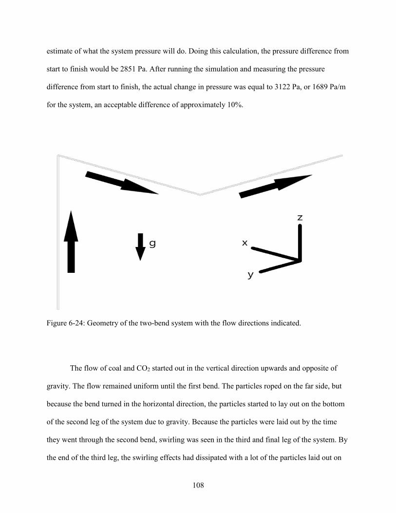
108

estimate of what the system pressure will do. Doing this calculation, the pressure difference from

start to finish would be 2851 Pa. After running the simulation and measuring the pressure

difference from start to finish, the actual change in pressure was equal to 3122 Pa, or 1689 Pa/m

for the system, an acceptable difference of approximately 10%.

The flow of coal and CO2 started out in the vertical direction upwards and opposite of

gravity. The flow remained uniform until the first bend. The particles roped on the far side, but

because the bend turned in the horizontal direction, the particles started to lay out on the bottom

of the second leg of the system due to gravity. Because the particles were laid out by the time

they went through the second bend, swirling was seen in the third and final leg of the system. By

the end of the third leg, the swirling effects had dissipated with a lot of the particles laid out on

Figure 6-24: Geometry of the two-bend system with the flow directions indicated.

109

the bottom of the pipe. Because of the additional distance the particles had to travel, the flow

varied quite a bit. The average coal mass flow rate was 0.003776 kg/s with a standard deviation

of 0.001871 kg/s, 49.5% of the average flow rate. The CO2 mass flow rate was more consistent

at 0.003780 kg/s and a standard deviation of 0.00005939 kg/s, 1.6% of the average flow rate.

110

7 PRESSURIZED FEED SYSTEM DESIGN

This chapter outlines a recommended conceptual pilot-scale feed system design as well as

some guidelines for designing a pressurized feed system.

7.1 Conceptual Pilot-Scale Feed System Design

The recommended conceptual design for the pressurized coal-feed system is the fluidized

bed design with a 5.08-cm (2-in) diameter uniform gas inlet, tapered 5.08-to-15.24-cm (2-to-6-

inch) diameter with a gas exit at the top of the hopper. To maximize run time of the reactor and

to minimize the times to refill the hopper with coal, the hopper should be made sufficiently large

to run for a full test session (typically eight hours). To run for eight hours based off a constant

coal mass flow rate of 0.00378 kg/s and utilizing the tapered diameter design in Figure 5-9, the

hopper should be approximately 4.73 meters (15.5 ft) tall. For a packing volume fraction of 0.6,

the height needed for the hopper would increase to 7.88 meters (25.8 ft). The packing volume

fraction of the actual coal to be used could be assessed by filling a 15-cm diameter pipe with a

given mass of coal to determine the mass of coal per unit height of the hopper. To reduce the

height of the hopper, the run time of the reactor could be reduced from eight to six or four hours.

To reduce the height of the hopper, but maintain the run time of eight hours, two hoppers could

be implemented of half the initial height with each carrying half the needed amount of coal.

Approximately 5 cm above the bottom of the bed there should be an outlet for coal and CO2 to

111

be transported through a 0.635-cm diameter exit pipe. The horizontal exit pipe should connect to

a vertical down pipe, which in turn should connect to the main 0.635-cm diameter horizontal

transport pipe. There should be a secondary inlet in this main transport pipe for dilution CO2 to

help transport diluted coal to the reactor. The piping dimensions from the hopper exit to the

reactor is uncertain because of the undetermined hopper and reactor placement, but segments of

pipe can be pieced together to create a full system between the hopper and reactor. Roping is

inevitable and may not be important because of small size of the coal and CO2 inlet area coming

into the reactor. If roping is found to significantly impact burner operation, a coal spreader or

similar device can be inserted just upstream of the burner to improve coal uniformity.

7.2 Guidelines for Pressurized System Design

Based on information identified in this research, several guidelines can be identified for

the design of dry-feed pressurized dense flow systems. A major assumption in this research was

implementing perfectly spherical particles (see Section 3.2). A higher velocity for transport

should be used to better model real coal particles. These design guidelines can be summarized as

follows:

1) Gravity fed systems are not likely to be effective due to their inability to motivate

sufficient coal flow into the feed system from the stationary coal storage, e.g.,

coal hopper, and their increased potential for coal bridging in the hopper.

2) Fluidized bed systems provide the ability to control coal mass flow rates leaving a

coal hopper and minimize chances of coal bridging or ratholing. Uniform gas

injection across the full diameter of the coal hopper base, as opposed to a single

112

jet in the center of the base, provides a more uniform fluidization of the coal

particles, increasing the steadiness of coal flow leaving the hopper.

3) A fluidized bed system in conjunction with a dilution gas flow provides the ability

to control particle flow rates and gas to particle flow ratios independently.

4) Particles in high pressure flow (e.g., 2 MPa) in horizontal pipes require higher gas

velocities to minimize layout than atmospheric systems.

5) Significant particle roping occurs for all bend radii. It is unlikely that a uniform

particle flow can be delivered to the burner. This may not be significant if the coal

inlet is small relative to the combustor diameter.

113

8 CONCLUSION

This chapter summarizes the main conclusions and insights from developing a CFD

model of a pressurized coal-feed system using the Barracuda CFD software and modeling

various design concepts and operating conditions. The feed system was designed to supply coal

to a reactor operating at 2.0 MPa (20 atm or 300 psi) with a 100 kWt firing rate. The feed system

needed to transport coal particles from a stationary bed, or hopper, to a combustor. The coal

mass flow rate needed to be maintained at 0.00378 kg/s and the CO2 used to transport the coal

needed to be maintained anywhere from 0.00378 to 0.00756 kg/s to provide a 1-2 gas-to-particle

mass loading ratio. Key results from the simulations are summarized below and illustrate that the

main research objective for this work, namely the development and use of a computational

model to design a conceptual pilot-scale pressurized coal-feed system, was achieved.

A mesh sensitivity study was conducted on a simple feed system geometry to assess the

level of mesh refinement required for the simulations. Results showed it was important to find

the right balance between a coarse and fine mesh. Specifically,

• The mesh should not be too coarse as geometry edges and curves can be poorly

represented and the cross-sectional area of the pipe will be inaccurate.

• The mesh needs to be fine enough to capture all of the physics and flow

characteristics in the system, but unlike common CFD practices, too fine of a

mesh in Barracuda will cause the cell size to approach the size of a computational

114

particle, or group of particles, resulting in inaccurate initialization of the particle

loading. The length of the smallest cell should not be smaller than five times the

smallest cell diameter.

• Refining the mesh beyond a relatively coarse level did not change the predicted

coal flow results.

Sub-model parameters can impact model predictions and can be changed to better reflect

real-life experiments, particle hardness, and pipe materials. Sensitivity studies were conducted to

determine parameter impact on coal mass flow rate leaving the pipe and the steadiness and

uniformity of the coal flow. Parameters evaluated included the close pack volume fraction,

maximum momentum redirection from collision, the normal-to-wall momentum retention, and

the tangent-to-wall momentum retention. Results showed that:

• For particle-to-wall interactions, the greater the normal-to-wall momentum

retention and the tangent-to-wall momentum retention values, the greater the coal

mass flow rate. Changing these values resulted in only a 2-3% difference in

predicted coal flow rate.

• Changing the particle-to-particle interaction parameter, maximum momentum

redirection from collision, resulted in a less than 1% change in predicted coal flow

values.

• Specification of the close pack volume fraction and the relative particle volume

fraction upon initialization was important because this determined how much of a

volume a particle occupies. Changing this parameter from 0.4 to 0.8 resulted in an

approximately 15% change in predicted coal flow rate.

115

• The recommended default Barracuda parameters were found to be reasonable and

provided consistent results for these simulations.

Two feed system design concepts were developed and tested throughout the course of

this research. The first was a gravity-fed concept and the second was a fluidized bed concept.

Simulation results showed the following.

• The gravity-fed system relied on gravity to move the particles from a stationary

standpipe (hopper) down into a moving gas stream. This concept was

unsuccessful due to insufficient coal flow from the standpipe into the gas stream.

Gravity forces were not sufficient to overcome the cohesion or packing forces on

the particles in the standpipe, particularly at the required high pressure. This also

resulted in low coal mass flow rates and unacceptably high CO2-to-coal mass flow

ratios. With the modified gravity-fed system the coal mass flow rate was

0.000324 kg/s with the lowest CO2-to-coal mass flow ratio of three, close to the 1-

2 ratio range. The greatest coal mass flow rate was 0.00145 kg/s, 38% of the

targeted value of 0.00378 kg/s with a CO2-to-coal mass flow ratio of 11.

• The fluidized bed concept relied on using part of the CO2 flow to fluidize particles

in the hopper (bed) to allow the particles to move more freely from the hopper

into the piping system. This concept was very successful. CO2 was introduced

uniformly at the base of the hopper at velocities calculated to produce either

minimum fluidization or bubbling fluidization. A fraction of this gas exited the

top of the hopper with the remainder conveying coal out of the hopper. The

amount of coal transported was a function of the difference between inlet and exit

CO2 flow. Additional CO2 was introduced in a horizontal pipe after the hopper to

116

dilute and pneumatically convey the coal through the feed system at calculated

velocities greater than the saltation velocity. Results showed that the fluidized

coal flow rate and dilution flow rate could be controlled independently, resulting

in significant flexibility in system design and operation. Coal flow rates greater

and less than the design value were possible (0.00378 kg/s), along with CO2-to-

coal mass flow ratios in the 1 to 2 range. One of the 5-to-15 diameter fluidized

bed cases (Case F13) reached a steady coal flow rate of 0.00376 kg/s and a

standard deviation of the flow rate over the average coal mass flow rate of 3.7%.

• Uniform gas injection across the full diameter of the coal hopper base, as opposed

to a single jet in the center of the base, provides a more uniform fluidization of the

coal particles, increasing the steadiness of the coal flow exiting the hopper.

• Nearly all coal flow results were found to be sufficiently steady for use with the

coal burner. Fluctuations of flow rate were quantified as the ratio of standard

deviation to average flow rate and were less than 5% at one-second time intervals.

Particle behavior in the piping system after the fluidized bed was simulated to assess

pressure drop, particle layout, and roping. Piping components modeled included 60.96-cm and

121.92-cm long horizontal pipe sections, and short (90°), medium (60.96 cm) and long (182.88

cm) pipe bend radii at different horizontal and vertical orientations. Flow steadiness, uniformity

(roping), and pressure drop were evaluated at CO2-to-coal mass flow ratios of 1 and 2. Results

showed that:

• With a greater gas mass flow rate and maintaining the same particle mass flow

rate, the steadiness of the flow increased.

117

• A greater gas mass flow rate reduced the layout of particles in the pipe and

maintained uniformity of the flow.

• Roping occurred whenever particle laden flow encountered a bend. The greater

the bend radius, the greater the roping of particles on the far side of the pipe.

• To reduce roping effects, straight piping should be added on after the bend to

allow the particles to redistribute themselves throughout the pipe.

• Particles in high pressure flow (e.g., 2 MPa) in horizontal pipes require higher gas

velocities to minimize lay out than atmospheric systems.

• Particles in high pressure flow exhibit more severe roping behavior around small

or large 90° bends than flow at lower pressures.

• Significant particle roping occurs for all bend radii. It is unlikely that a uniform



• For the same CO2 mass flow rates, the pressure drop per unit length was always

greatest across the larger radius bend (0.3175-cm, 60.96-cm, and 182.88-cm). For

the same geometry, the pressure drop per unit length was always greatest with the

higher CO2 mass flow rate (1-to-1 and 2-to-1 gas-to-particle mass ratio).

• A simple methodology was identified to estimate pressure drop for different

piping system configurations based on the piping components simulated.

The recommended conceptual design for the pressurized coal-feed system is the fluidized

bed design with a 5.08-cm (2-in) diameter uniform bed inlet tapering to the 15.24-cm (6-in)

118

diameter. The hopper will hold enough coal to run the reactor for eight hours. A steady coal mass

flow rate of 0.00378 kg/s will be delivered to the reactor with a varying CO2 flow rate to adjust

the CO2-to-coal mass ratio. Depending on the packing fraction of the coal, the height of the

hopper will range from 4.73 to 7.88 meters tall (15.5 to 25.8 feet). This height is adjustable

depending also on the run time of the reactor and if two hoppers are implemented. The coal and

CO2 leaving the hopper will be transported through a 0.635-cm diameter pipe to the reactor. A

secondary CO2 inlet for dilution will be introduced to help transport and control the CO2-to-coal

mass flow ratio. Pipe segments will be pieced together to create the full system. Roping will

occur no matter the bend radius. A coal spreader or similar device can be inserted upstream of

the burner to improve coal uniformity if roping proves to be a problem.

Based on simulation results for the different design concepts and piping components, five

design guidelines were identified to guide current and future pressurized feed system designs.

These guidelines are:

1) Gravity fed systems are not likely to be effective due to their inability to motivate

sufficient coal flow into the feed system from the stationary coal storage, e.g.,

coal hopper, and their increased potential for coal bridging in the hopper.

2) Fluidized bed systems provide the ability to control coal mass flow rates leaving a

coal hopper and minimize chances of coal bridging or ratholing. Uniform gas

injection across the full diameter of the coal hopper base, as opposed to a single

jet in the center of the base, provides a more uniform fluidization of the coal

particles, increasing the steadiness of coal flow leaving the hopper.

3) A fluidized bed system in conjunction with a dilution gas flow provides the ability

to control particle flow rates and gas to particle flow ratios independently.

119

4) Particles in high pressure flow (e.g., 2 MPa) in horizontal pipes require higher gas

velocities to minimize layout than atmospheric systems.

5) Significant particle roping occurs for all bend radii. It is unlikely that a uniform



120

REFERENCES

[1] T. Hodge, "Coal May Surpass Natural Gas as Most Common Electricity Generation Fuel This Winter," U.S. Energy Information Administration, 2016.

[2] Union of Concerned Scientists, "Coal and Air Pollution," Union of ConcernedScientists, 19 December 2017. [Online]. Available: https://www.ucsusa.org/clean-energy/coal-and-other-fossil-fuels/coal-air-pollution#.W6J7YWhKiUk. [Accessed 19September 2018].

[3] J. Hong, G. Chaudhry, J. G. Brisson, R. Field, M. Gazzino and A. F. Ghoniem,"Analysis of Oxy-Fuel Combustion Power Cycle Utilizing a Pressurized Coal Combustor,"Energy, vol. 34, pp. 1332-1340, 2009.

[4] L. Chen, S. Z. Yong and A. F. Ghoniem, "Oxy-fuel combustion of pulverized coal:characterization, fundamentals, stabilization and CFD modeling," Prog Energy CombustSci, vol. 38, pp. 156-214, 2012.

[5] B. Yan, "Study on the rheology of coal-oil slurries during heating at high pressure,"International Journal of Coal Science & Technology, vol. 4, no. 3, pp. 274-280, 2017.

[6] Y. Ren, D. Zhang and J. Gao, "Viscosity variations of coal-oil slurry under hightemperature and high pressure during heating process," Fuel Processing Technology, vol.92, no. 12, pp. 2272-2277, 2011.

[7] P. Basu, Circulating Fluidized Bed Boilers: Design, Operation and Maintenance,Springer International Publishing, 2015, pp. 19-20.

[8] J. R. Grace, Fluidized Bed Hydrodynamics, G. Hestroni, Ed., Washington:Hemisphere, 1982, pp. 8-5 - 8-64.

[9] A. R. Abrahamsen and D. Geldart, "Behaviour of gas-fluidized beds of finepowders part I. Homogeneous expansion," Powder Technology, vol. 35, p. 26, 1980.

[10] L. M. Gomes and A. L. A. Mesquita, "Effect of particle size and sphericity on thepickup velocity in horizontal pneumatic conveying," Chemical Engineering Science, vol.104, pp. 780-789, 2013.

[11] J. Shabanian and J. Chaouki, "Effects of temperature, pressure, and interparticleforces on the hydrodynamics of a gas-solid fluidized bed," Chemical Engineering Journal,vol. 313, pp. 580-590, 2017.

121

[12] W. Pu, C. Zhao, Y. Xiong, C. Liang, X. Chen, P. Lu and C. Fan, "Numerical simulation on dense phase pneumatic conveying of pulverized coal in horizontal pipe at high pressure," Chemical Engineering Science, vol. 65, pp. 2500-2512, 2010.

[13] H. Kalman, A. Satran, D. Meir and E. Rabinovich, "Pickup (critical) velocity of particles," Powder Technology, vol. 160, pp. 103-113, 2005.

[14] G. E. Klinzing, F. Rizk, R. Marcus and L. S. Leung, Pneumatic Conveying of Solids: A theoretical and practical approach, 3 ed., 2009, pp. 187-188.

[15] F. J. Cabrejos and G. E. Klinzing, "Incipient motion of solid particles in horizontal pneumatic conveying," Powder Technology, vol. 72, pp. 51-61, 1992.

[16] E. Rabinovich and H. Kalman, "Generalized master curve for threshold superficial velocites in particle-fluid systems," Powder Technology, vol. 183, pp. 304-313, 2008.

[17] G. E. Klinzing, "Pneumatic conveying: transport solutions, pitfalls, and measurements," Handbook of Conveying and Handling of Particulate Solids, pp. 291-301, 2001.

[18] K. S. Hayden and J. S. Curtis, "Effect of particle characteristics on particle pickup velocity," Powder Technology, vol. 131, no. 1, pp. 7-14, 2003.

[19] L. Cai, S. Liu, X. Pan, X. Guiling, Y. Gaoyang, C. Xiaoping and Z. Changsui, "Comparison of pressure drops through different bends in dense-phase pneumatic conveying system at high pressure," Experimental Thermal and Fluid Science, vol. 57, pp. 11-19, 2014.

[20] Y. Lu, Z. Tong, D. H. Glass, W. J. Easson and M. Ye, "Experimental and numberical study of particle velocity distribution in the vertical pipe after a 90° elbow," Powder Technology, vol. 314, pp. 500-509, 2017.

[21] H. Akilli, E. K. Levy and B. Sahin, "Gas-solid flow behavior in a horizontal pipe after a 90° vertical-to-horizontal elbow," Powder Technolgy, vol. 116, pp. 43-52, 2001.

[22] B. V. Reactor, "Barracuda Virtual Reactor User Manual," Barracuda Virtual Reactor, 2018. [Online]. Available: http://cpfd-software.com/user-manual/index. [Accessed 2018].

[23] A. Abbasi, P. E. Ege and H. I. de Lasa, "CPFD simulation of a fast fluidized bed steam coal gasifier feeding section," Chemical Engineering Journal, vol. 174, no. 1, pp. 341-350, 2011.

122

[24] S. Yin, W. Zhong, B. Jin and J. Fan, "Modeling on the hydrodynamics of pressurized high-flux circulating fluidized beds (PHFCFBs) by Eulerian-Lagrangian approach," Powder Technology, vol. 259, pp. 52-64, 2014.

[25] H. Liu, R. J. Cattolica and R. Seiser, "Operating parameter effects on the solids circulation rate in the CFD simulation of a dual fluidized-bed gasification system," Chemical Engineering Science, vol. 169, pp. 235-245, 2017.

[26] Y. Liang, Y. Zhang, T. Li and C. Lu, "A critical validation study on CPFD model in simulating gas-solid bubbling fluidized beds," Powder Technology, vol. 263, pp. 121-134, 2014.

[27] J. M. Weber, K. J. Layfield, D. T. Van Essendelft and J. S. Mei, "Fluid bed characterication using Electrical Capacitance Volume Tomography (ECVT), compared to CPFD Software's Baracuda," Powder Technology, vol. 250, pp. 138-146, 2013.

[28] K. Li, S. B. Kuang, R. H. Pan and A. B. Yu, "Numerical Study of horizontal pneumatic conveying: effect of material properties," Powder Technology, vol. 251, pp. 15-24, 2014.

[29] D. Geldart and S. J. Ling, "Dense phase conveying of fine coal at high total pressures," Powder Technology, vol. 62, pp. 243-252, 1990.

[30] W. K. Hiromi Ariyaratne, C. Ratnayake and M. C. Melaaen, "Application of the MP-PIC method for predicting pneumatic conveying characteristics of dilute phase flows," Powder Technology, vol. 310, pp. 318-328, 2017.

[31] Q. Wang, H. Yang, P. Wang, J. Lu, Q. Liu, H. Zhang, L. Wei and M. Zhang, "Application of CPFD method in the simulation of a circulating fluidized bed with a loop seal, part I—Determination of modeling parameters," Powder Technology, vol. 253, pp. 814-821, 2014.

[32] R. Chhabra, L. Agarwal, N. Sinha and e. al., "Drag on non-spherical particles: an evaluation of available methods," Powder Technonlogy, vol. 101, pp. 288-295, 1999.

[33] J. Militzer, J. Kan, F. Hamdullahpur and e. al., "Drag Coefficient For Axisymmetric Flow Around Individual Spheroidal Particles," Powder Technology, vol. 57, pp. 193-195, 1989.

[34] P. J. Blaser and G. Corina, "Validation and application of computational modeling to reduce erosion in a circulating fluidized bed boiler," International Journal of Chemical Reactor Engineering, vol. 10, no. 1, pp. 1515-1542, 2012.

123

[35] Tony, "Fluidization Process at Different Stages," SaintyCo, 2018. [Online]. Available: https://www.saintytec.com/fluid-bed-granulation-process/fluidization-process-at-different-stages/. [Accessed 2018].

conceptual design of a pilot-scale pressurized coal-feed

Documents