vii

Contents

Acknowledgments : : : : : : : : : : : : : : : : : : : : : : : : : : : : : : ii

Dedication : : : : : : : : : : : : : : : : : : : : : : : : : : : : : : : : : : : iv

Abstract : : : : : : : : : : : : : : : : : : : : : : : : : : : : : : : : : : : : v

Contents : : : : : : : : : : : : : : : : : : : : : : : : : : : : : : : : : : : : vii

1 General Introduction : : : : : : : : : : : : : : : : : : : : : : : : : : 1

1.1 Overview and Motivation : : : : : : : : : : : : : : : : : : : : : : : : 1

1.2 Objective : : : : : : : : : : : : : : : : : : : : : : : : : : : : : : : : 4

1.3 Organization : : : : : : : : : : : : : : : : : : : : : : : : : : : : : : 5

2 Methods Used in This Study : : : : : : : : : : : : : : : : : : : : : 8

2.1 Introduction : : : : : : : : : : : : : : : : : : : : : : : : : : : : : : : 8

2.2 Linearized least-squares inversion : : : : : : : : : : : : : : : : : : : 9

2.3 Optimization by simulated annealing : : : : : : : : : : : : : : : : : 12

2.3.1 Determination of the annealing parameters : : : : : : : : : : 17

2.4 Pre-stack Migration : : : : : : : : : : : : : : : : : : : : : : : : : : : 21

3 Velocity Estimation and Imaging by Optimization of First-Arrival

viii

Times : : : : : : : : : : : : : : : : : : : : : : : : : : : : : : : : : : : 26

3.1 Abstract : : : : : : : : : : : : : : : : : : : : : : : : : : : : : : : : : 26

3.2 Introduction : : : : : : : : : : : : : : : : : : : : : : : : : : : : : : : 27

3.3 Results From Synthetic Models : : : : : : : : : : : : : : : : : : : : 30

3.3.1 Low-velocity basin : : : : : : : : : : : : : : : : : : : : : : : 31

3.3.2 High-velocity intrusion : : : : : : : : : : : : : : : : : : : : : 37

3.3.3 Low-velocity layer model : : : : : : : : : : : : : : : : : : : : 42

3.4 Shallow-Crustal Structure In The Death Valley Region of California 44

3.4.1 Velocity Estimation Using COCORP DV Line 9 Data : : : : 46

3.4.2 Velocity Estimates Under COCORP DV Line 10 : : : : : : : 49

3.4.3 Velocity Estimates Under COCORP DV Line 11 : : : : : : : 52

3.4.4 Inferences Based on Shallow Velocities in Death Valley : : : 55

3.5 Imaging the o�shore Hosgri Fault, California : : : : : : : : : : : : : 57

3.5.1 Optimization Results Using Picks From EDGE RU-3 Line : 58

3.6 Sub-surface Geometry of The Mojave Segment of the San Andreas

Fault : : : : : : : : : : : : : : : : : : : : : : : : : : : : : : : : : : : 62

3.6.1 Velocity Optimization: Results and Inferences : : : : : : : : 64

3.6.2 Pre-stack Imaging: Results and Inferences : : : : : : : : : : 70

3.7 Conclusions : : : : : : : : : : : : : : : : : : : : : : : : : : : : : : : 72

4 Estimation of Velocities and Re ector Characteristics From Re-

ection Travel Times Using a Nonlinear Optimization Method 75

ix

4.1 Abstract : : : : : : : : : : : : : : : : : : : : : : : : : : : : : : : : : 75

4.2 Introduction : : : : : : : : : : : : : : : : : : : : : : : : : : : : : : : 76

4.3 Re ection Travel Time Calculation : : : : : : : : : : : : : : : : : : 79

4.4 Results : : : : : : : : : : : : : : : : : : : : : : : : : : : : : : : : : : 79

4.4.1 Optimization results of the three box model : : : : : : : : : 81

4.4.2 Optimization results of the lateral gradient model : : : : : : 84

4.5 Comparison with a linearized inversion scheme : : : : : : : : : : : : 86

4.6 Imaging the Garlock Fault, Cantil Basin : : : : : : : : : : : : : : : 88

4.6.1 Results of the travel time inversion : : : : : : : : : : : : : : 92

4.6.2 Including First-Arrival Travel Times : : : : : : : : : : : : : 101

4.7 Conclusions : : : : : : : : : : : : : : : : : : : : : : : : : : : : : : : 102

5 A Combined First-Arrival Travel Time and Re ection Coherency

Optimization Approach to Velocity Estimation : : : : : : : : : 106

5.1 Abstract : : : : : : : : : : : : : : : : : : : : : : : : : : : : : : : : : 106

5.2 Introduction : : : : : : : : : : : : : : : : : : : : : : : : : : : : : : : 107

5.3 Method : : : : : : : : : : : : : : : : : : : : : : : : : : : : : : : : : 109

5.4 Results From Synthetic Test : : : : : : : : : : : : : : : : : : : : : : 112

5.5 Results Using Data From COCORP Line 1 : : : : : : : : : : : : : : 116

5.6 Results Using Data From COCORP Line 5 : : : : : : : : : : : : : : 116

5.7 Inferences : : : : : : : : : : : : : : : : : : : : : : : : : : : : : : : : 119

6 Conclusions and Suggestions : : : : : : : : : : : : : : : : : : : : : 122

x

6.1 Summary : : : : : : : : : : : : : : : : : : : : : : : : : : : : : : : : 122

6.2 Suggestions : : : : : : : : : : : : : : : : : : : : : : : : : : : : : : : 127

7 References : : : : : : : : : : : : : : : : : : : : : : : : : : : : : : : : 130

1

Chapter 1

General Introduction

1.1 Overview and Motivation

Velocity estimation is one of the main objectives of seismic re ection data process-

ing and an integral part of seismic interpretation. Knowledge of seismic velocities

is essential to convert sections recorded in time on the earth's surface to depth

sections. These sections map the re ecting horizons which the interpreter then

uses to derive structural information (Dix, 1955; Claerbout, 1985).

Conventional velocity analysis generally falls into two categories, based on the

aspect of the seismic information they use. These methods are often applied se-

quentially. The �rst utilizes the time di�erence aspect of the data and the processes

are called \normal move out" (NMO) and \stacking"; the second involves com-

puting the \velocity spectrum", which uses the coherency aspect of the data. The

NMO relation represents the time di�erence between travel times at a given o�set

and at zero o�set. The velocity required to collapse data to zero o�set gives the

normal move out velocity. Thus, it assumes all traces obey the hyperbolic travel

time equation. This holds good for short o�sets (a maximum source-receiver o�set

2

of 1 km) and in a medium composed of only gently dipping re ectors but breaks

down for layer boundaries having arbitrary shapes. Estimation of stacking veloc-

ities is based on the hyperbola that best �ts data over the entire spread length

(Yilmaz, 1987). Generally, NMO correction velocities are considered equivalent to

stacking velocities.

The second commonly used method is to compute the velocity spectrum. This

involves calculating signal coherency on common mid point (CMP) gathers along a

hyperbolic trajectory, using the NMO o�set versus time relation. On completion,

one ends up with a map of coherency for di�erent velocities at di�erent two-way

zero-o�set times. Stacking velocities are estimated from the velocity spectrum by

choosing the velocity function that produces the highest coherency at times with

signi�cant event amplitudes.

Both of these conventional approaches, reliant on the NMO relation, tend to

become unreliable in areas where velocity undergoes rapid lateral variations (more

than 10-20% change) and re ectors dip arbitrarily (steeper than 5�100). Moreover,

under these conditions, the stacking velocities do not represent the velocity of the

medium. One has to assume horizontal strati�cation to deduce parameters like

root mean square (rms) velocity, and interval velocities (Dix, 1965).

To address these shortcomings numerous travel time inversion schemes have

been developed. Inversion of �rst-arrival times picked o� multi-o�set seismic data

give detailed shallow velocity structure. Several linearized inversion schemes have

been developed to solve this problem (e.g. Hampson and Russell, 1984; Docherty,

3

1992; Simmons and Backus, 1992). These velocities can be used either in \statics"

corrections (Farrell and Euwema, 1994), as part of conventional seismic processing,

or as an input to a pre-stack migration process that directly images re ectors (Louie

and Qin, 1991). Travel time inversion is a nonlinear process, where perturbation

of the velocity �eld alters the ray paths through it. The methods in use linearize

this nonlinear problem and achieve convergence through iteration. A drawback of

this approach is that the solution becomes initial-model dependent. I address this

problem by adapting a nonlinear optimization method to estimate velocities from

�rst-arrival times.

Another method to obtain information about re ector locations is to invert

re ection arrival times. Re ection travel times provide velocity information from

deeper horizons than �rst arrivals and about the re ector itself. Re ection times

depend on both the velocity and the depth of re ectors, making re ection travel

time inversion a nonlinear process. Methods that tackle this problem generally

fall into two categories. The �rst involves parameterizing both velocity and re ec-

tor depth and performing a joint inversion (e.g., Bishop et al., 1985; Farra and

Madariaga, 1988). The second approach is to use a migration technique to image

the re ector with the existing velocity �eld, then update the velocity keeping the

re ector �xed (e.g., Bording et al., 1987; Stork and Clayton, 1987).

The above methods involved local linearization of the problem and require the

starting model to be close to the solution. To alleviate this drawback, I formulate

another Monte Carlo based optimization that avoids linearization. I design it to

4

be initial-model independent and able to simultaneously reconstruct velocities and

re ector location from re ection times. Thus it can recover the dip and length of

the re ecting horizon. A major advantage of using a Monte-Carlo based search

technique is the exibility in model mis�t measures and model parameterization.

1.2 Objective

The main objective of this thesis is to document a nonlinear optimization technique

that can reconstruct velocities from travel times recorded by surface multi-o�set

seismic survey data. It is a Monte Carlo method, speci�cally, generalized simulated-

annealing, essentially comprised of repeated forward modeling. Hence I prefer to

use the term \optimization" rather than \inversion" to describe the method.

As alluded to in the Overview, I adapt the method to estimate velocities from

both �rst-arrival and re ection travel times. I also attempt to circumvent the

question of re ector depth versus velocity ambiguity, inherent to re ection travel

time problems by including amplitude information in the optimization.

The prime objective of seismic processing is imaging re ectors. I demonstrate

how velocities obtained from �rst-arrival time optimization can be used in a pre-

stack migration to image re ectors. I also show how, using re ection times, one

can estimate both velocities and re ector characteristics.

5

1.3 Organization

This thesis summarizes the e�orts to adapt a nonlinear optimization method to

obtain information about the earth's crust using travel time and amplitude infor-

mation. It can be viewed as an attempt to link imaging with velocity analysis.

Each chapter deals with the use of di�erent types of information contained in seis-

mic survey data. For each approach, I perform synthetic tests before optimally

�tting real data sets. If applicable, the results are compared to prior models, and

tectonic or geologic interpretations are made.

In Chapter 2, I brie y explain all the methods I use that are central to the

thesis. Included are the generalized simulating-annealing method, a linearized

inversion approach, and pre-stack migration based on the Kirchho�-sum approach.

In the subsequent Chapters, I only elaborate on speci�c adaptations to the general

approaches developed in Chapter 2.

In Chapter 3, the simulated-annealing method is used to estimate high-resolution

near surface velocities from �rst-arrival times (Pullammanappallil and Louie, 1994).

The algorithm is tested on synthetic models and compared with a linearized in-

version scheme. I show that the optimization procedure can recover rapid lateral

variation in velocities. To achieve this I use �rst-arrival times picked o� three sets

of �eld gathers. The �rst is from a marine re ection data set collected by the

EDGE consortium across the Hosgri fault, o�shore California (Figure 3.15); the

second is from the Consortium for Continental Re ection Pro�ling (COCORP)

6

Death Valley lines 9, 10, and 11 (Figure 3.9); and the third is a sub-set of the CO-

CORP Mojave line 1 data that crosses the San Andreas fault in southern California

(Figure 3.18). Once the velocities are derived, they are used as an initial velocity

model in a pre-stack migration process imaging re ectors and this procedure is

demonstrated using data sets 1 and 2.

Pre-stack migration of the marine data set images the near-vertical trace of

the Hosgri fault. The migration was performed by Honjas (1993) as part of his

M.S. thesis. He also performed a post-stack migration on the shot gathers to

image the horizontal re ectors. The resulting structure models allowed him to

infer the history of motion on the fault. Velocity models from the COCORP

Death Valley lines supplement existing velocity models for the shallow crust (e.g.:

Geist and Brocher, 1987). They also provide some constraints for the nature

of extension that are operating in the region (Pullammanappallil et al., 1994).

Accurate velocity estimation using picks from COCORP Mojave line 1 helps image

the subsurface geometry of the San Andreas fault (Louie and Pullammanappallil,

1994). This geometry, in conjunction with seismicity data, help us to delineate

the fault location at depth. The results do not indicate the presence of the often

hypothesized crustal-penetrating low-velocity zone in this region.

In Chapter 4, I extend the nonlinear optimization scheme to obtain velocities,

and re ector depths and lengths from seismic re ection travel time picks (Pullam-

manappallil and Louie, 1993). I also describe a �nite-di�erence based method to

�nd re ection times through a velocity model that is deterministic and computa-

7

tionally faster than ray-tracing. I compare and contrast the nonlinear optimization

with a linearized least-squares inversion using synthetic models to highlight the

initial-model dependence of the linear scheme.

The method is used to image the Garlock fault, whose geometry at depth is

poorly known, with data from shot gathers recorded by COCORP (Line 5, Figure

4.7). I also discuss a method of resolution analysis for optimization that appears

to be more relevant than the standard approach of computing a resolution ma-

trix. This method, combined with a statistical analysis of the model parameters

obtained, helps to estimate the uncertainty associated with the velocities and re-

ector position.

In Chapter 5, I describe how the optimization scheme is modi�ed to include

amplitude information. The method also provides a possible solution to the often

di�cult procedure of picking re ected arrivals from a �eld record. The amplitude

information is included by invoking the idea that the arrivals re ected from a

structure will have a maximum \coherency" from trace to trace in the data (Landa

et al., 1989). I demonstrate the application of coherency using synthetic data, the

shot gathers from COCORP line 5 that were put to use in Chapter 3, and the

data recorded along COCORP line 1 used in Chapter 4. Including the coherency

criterion increases the depth of well-resolved velocities and consequently improves

the imaging of re ectors.

In Chapter 6, I summarize the results, discuss the merits and drawbacks of the

nonlinear optimization method, and make some suggestions for future research.

8

Chapter 2

Methods Used in This Study

2.1 Introduction

This chapter presents an overview of the methods used during the course of this

dissertation work. The nonlinear optimization technique is central to the thesis

and its performance is compared with a linearized least-squares technique in all

the applications (i.e., when using �rst-arrival times and re ection travel times).

Velocities obtained from �rst-arrival travel time and combined coherency�travel-

time optimization are used in pre-stack migrations to image re ectors.

I �rst discuss the linearized velocity and re ector depth inversion from re ection

time picks. It helps explain the data and model terminology I use throughout

this thesis, and comes most directly from previous work by others. I then can

alter it for the linear inversion for velocity only from �rst-arrival picks. Although

I implemented the linearized methods primarily for the purpose of comparison

against the non-linear optimizations, they are for some cases robust and useful

methods in their own right. Thus I will carefully develop my implementation of

them, and explain their strengths and weaknesses.

9

2.2 Linearized least-squares inversion

Re ection travel times, t, are a nonlinear function of the slowness, s of the medium,

and the re ector depth, d, which can be expressed as:

t = F (s; d) : (1)

One can expand F (s; d) about an initial model, (s0; d0), resulting in

t = F (s0; d0) + (GsjGd)

0BBB@

�s

�d

1CCCA+Ok�s2k+Ok�d2k : (2)

The matrices Gs and Gd contain partial derivatives of the travel times with respect

to the slowness and depth respectively. �s and �d are the slowness and re ector

depth correction vectors. O indicates higher order terms that are assumed negli-

gible. This assumption helps to keep the computation time tractable. Denoting

the model parameters, s and d, as m and Gm as (GsjGd), one can write the above

equation as

t = F (m0) +Gm�m+Ok�m2k : (3)

Neglecting the higher-order terms:

t� F (m0) � Gm�m (4)

10

This system is generally solved for m in a linear least-squares framework (Jack-

son, 1972; Wiggins, 1972). I use a singular value decomposition to achieve this,

following Press et al. (1988). Instead of solving for the perturbations to the model

parameters, I compute a new model during each iteration in the manner of Shaw

and Orcutt (1985). Following their formalism I add the product Gmm0 to both

sides of equation (4)

t� F (m0) +Gmm0 � Gmm : (5)

This allows for easy implementation of constraints such as smoothness on the model

parameters, m. The objective is to iteratively minimize the travel time residual,

R0 (= t� F (m0)). To speed up convergence and stabilize the inversion I smooth

the slowness perturbations using a Laplacian operator (Lees and Crosson, 1989)

and the re ector depth by a second di�erence operator (Ammon et al., 1990). The

matrix equations can now be written in iterative form (Ammon and Vidale, 1992)

as, 0BBBBBBBB@

Ri�1

0

0

1CCCCCCCCA+

0BBBBBBBB@

Gmmi�1

0

0

1CCCCCCCCA=

0BBBBBBBB@

Gm

��

��

1CCCCCCCCAmi : (6)

mi is the vector containing the model parameters after the ith iteration, mi�1

the solution from the previous iteration, and Gm is calculated using mi�1. �

and � are the weighting factors for the smoothness matrix for the slowness and

11

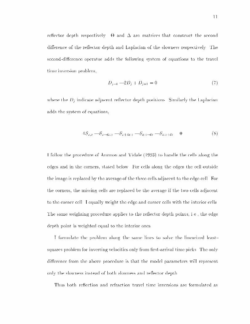
re ector depth respectively. � and � are matrices that construct the second

di�erence of the re ector depth and Laplacian of the slowness respectively. The

second-di�erence operator adds the following system of equations to the travel

time inversion problem,

Dj�1 � 2Dj +Dj+1 = 0 (7)

where the Dj indicate adjacent re ector depth positions. Similarly the Laplacian

adds the system of equations,

4Sx;z � Sx�dx;z � Sx+dx;z � Sx;z�dz � Sx;z+dz = 0 (8)

I follow the procedure of Ammon and Vidale (1993) to handle the cells along the

edges and in the corners, stated below. For cells along the edges the cell outside

the image is replaced by the average of the three cells adjacent to the edge cell. For

the corners, the missing cells are replaced be the average if the two cells adjacent

to the corner cell. I equally weight the edge and corner cells with the interior cells.

The same weighting procedure applies to the re ector depth points, i.e., the edge

depth point is weighted equal to the interior ones.

I formulate the problem along the same lines to solve the linearized least-

squares problem for inverting velocities only from �rst-arrival time picks. The only

di�erence from the above procedure is that the model parameters will represent

only the slowness instead of both slowness and re ector depth.

Thus both re ection and refraction travel time inversions are formulated as

12

linearized least-squares problems. These approaches are used on synthetic models

to estimate velocities in Chapter 3, and velocity and re ector depth in Chapter 4.

In all cases, I compare their performance against a nonlinear optimization method,

which is described in the next section.

2.3 Optimization by simulated annealing

Simulated annealing is a Monte Carlo optimization method that mimics the phys-

ical process by which a crystal grows from a melt. One can relate crystallization

to optimization by characterizing the nonlinear inversion as a transformation from

disorder (initial model) to order (the solution). Kirkpatrick et al. (1983) were the

�rst to introduce the simulated-annealing method of optimization. Their method

is a variant of a Monte Carlo integration procedure due to Metropolis et al. (1953).

While Metropolis et al. sampled a Gibbs distribution at constant \temperature",

the Kirkpatrick et al. algorithm included a temperature schedule promoting e�-

cient searching.

This method avoids local linearization and does not require the calculation

of partial derivatives. Ideally, it has the ability to test a series of local minima

in search of the global minimum. In general, the method of simulated annealing

consists of two functional relationships:

1. Pc: Probability for acceptance of a new state of the model given the imme-

diately previous model state.

13

2. T (i): schedule of the \temperature" T for \annealing" in annealing-time

steps (iterations) i, for changing the volatility or uctuations of the previous

probability density.

The acceptance probability is based on the chances of obtaining a new state

with \energy" Ei+1 relative to a previous state with \energy" Ei and is given as

Pc = exp(��E

T) (9)

This represents a Gibbs distribution (Metropolis et al. 1953; Ingber, 1993). Kirk-

patrick et al. (1983) proposed an important link between physics and statistics by

letting the energy represent an objective function in an optimization problem.

Rothman (1985, 1986) showed that large non-linear problems encountered in

re ection seismology can be expressed as Markov chains, in which the equilibrium

distribution is the Gibbs distribution of statistical mechanics. This equivalence in

distributions leads to the statement that in theory, using a probability distribution

shown in equation (9), one should be able to sample all states of the system. This

translates to saying that I should be able to sample the model space extensively,

facilitating the �nding of the global minimum.

It can also be shown that the acceptance probability distribution is equivalent

to the posterior probability density function. In nonlinear least squares formal-

ization, one can denote the posterior probability density in model space, �M(m),

14

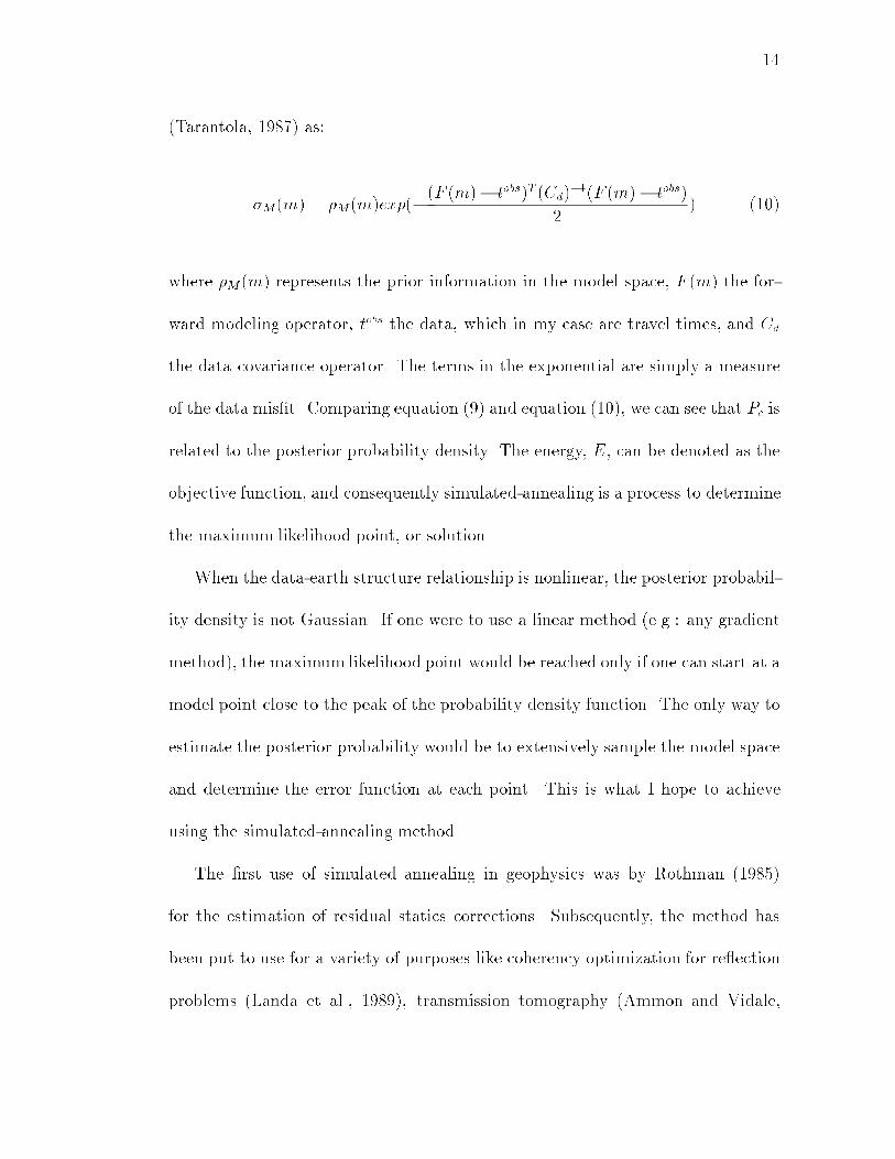
(Tarantola, 1987) as:

�M(m) = �M(m)exp(�(F (m)� tobs)T (Cd)�1(F (m)� tobs)

2) (10)

where �M (m) represents the prior information in the model space, F (m) the for-

ward modeling operator, tobs the data, which in my case are travel times, and Cd

the data covariance operator. The terms in the exponential are simply a measure

of the data mis�t. Comparing equation (9) and equation (10), we can see that Pc is

related to the posterior probability density. The energy, E, can be denoted as the

objective function, and consequently simulated-annealing is a process to determine

the maximum likelihood point, or solution.

When the data-earth structure relationship is nonlinear, the posterior probabil-

ity density is not Gaussian. If one were to use a linear method (e.g.: any gradient

method), the maximum likelihood point would be reached only if one can start at a

model point close to the peak of the probability density function. The only way to

estimate the posterior probability would be to extensively sample the model space

and determine the error function at each point. This is what I hope to achieve

using the simulated-annealing method.

The �rst use of simulated annealing in geophysics was by Rothman (1985)

for the estimation of residual statics corrections. Subsequently, the method has

been put to use for a variety of purposes like coherency optimization for re ection

problems (Landa et al., 1989), transmission tomography (Ammon and Vidale,

15

1990), and seismic waveform inversion (Sen and Sto�a, 1991).

I make use of a variation of this optimization process called generalized sim-

ulated annealing (Bohachevsky et al., 1986; Landa et al., 1989). The algorithm

essentially comprises the following steps:

1. Compute travel times through an initial model. Determine the least-square

error, E0. For any iteration i, I can de�ne the least-square error (which is

the objective function) as:

Ei =1

n

nXj=1

(tobsj � tcalj )2 (11)

where n is the number of observations, j denotes each observation, and tobs

and tcal are the observed (data) and calculated travel times respectively.

2. The next step is to perturb the model. To preserve the nonlinearity of the

re ection travel-time optimization, I carry out simultaneous perturbations of

the medium velocity and the re ector depth. I perturb the velocity by adding

random-sized boxes, followed by smoothing by averaging over four adjacent

cells. The boxes can vary between one cell size and the entire model size.

To perturb the re ector I add random-length lines that are smoothed by

averaging adjacent nodes. Again, the added lines can be as small as one grid

spacing or as long as the length of the model. Following the perturbation, I

compute the new least-square error E1.

16

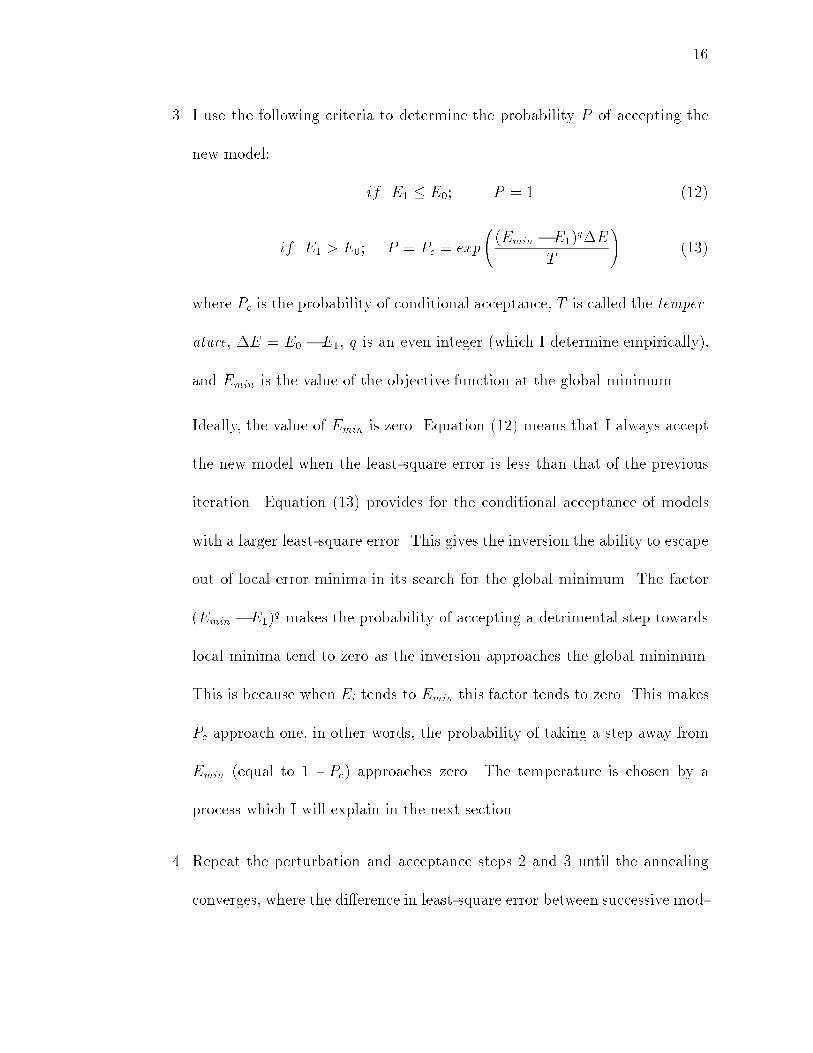
3. I use the following criteria to determine the probability P of accepting the

new model:

if E1 � E0; P = 1 (12)

if E1 > E0; P = Pc = exp

(Emin � E1)q�E

T

!(13)

where Pc is the probability of conditional acceptance, T is called the temper-

ature, �E = E0 � E1, q is an even integer (which I determine empirically),

and Emin is the value of the objective function at the global minimum.

Ideally, the value of Emin is zero. Equation (12) means that I always accept

the new model when the least-square error is less than that of the previous

iteration. Equation (13) provides for the conditional acceptance of models

with a larger least-square error. This gives the inversion the ability to escape

out of local error minima in its search for the global minimum. The factor

(Emin � E1)q makes the probability of accepting a detrimental step towards

local minima tend to zero as the inversion approaches the global minimum.

This is because when Ei tends to Emin this factor tends to zero. This makes

Pc approach one, in other words, the probability of taking a step away from

Emin (equal to 1 - Pc) approaches zero. The temperature is chosen by a

process which I will explain in the next section.

4. Repeat the perturbation and acceptance steps 2 and 3 until the annealing

converges, where the di�erence in least-square error between successive mod-

17

els and the probability of accepting new models becomes very small. One

discerns the latter condition when there are a large number of iterations

(50,000 or more) over which no model is accepted. In my tests this num-

ber is approximately 30 to 40 times the number of model parameters being

determined.

Simulated annealing requires only repeated forward modeling. Rothman (1985)

showed that using the acceptance probability function, Pc, makes the algorithm

a Markov chain with a Gibbs equilibrium probabilities. A Markov chain is \irre-

ducible" and \aperiodic". Irreducibility implies that every state of a parameter

can be reached, while aperiodicity means that the system exhibits a distribution of

states that is independent of time. These properties make the simulated-annealing

method well-suited to sample the extensive model-space encountered in the non-

linear problems I will be dealing with.

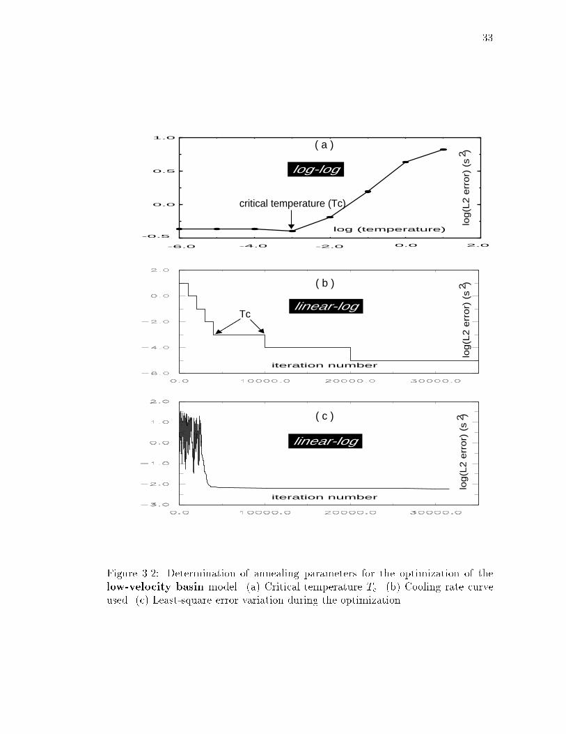
2.3.1 Determination of the annealing parameters

The convergence of the simulated-annealing optimization is sensitive to the value of

q and the rate of cooling. The rate of cooling refers to the variation of parameter T

with iteration i to aid convergence. One iteration can include one perturbation of

both velocity and re ector depth. Rothman (1986) found that simulated annealing

�nds the global minimumwhen one starts at a high temperature, rapidly cools to a

lower temperature,and then performs a number of iterations at that temperature.

This low temperature, referred to as the critical temperature (Tc), must be high

18

enough to allow the inversion to escape local minima, but low enough to ensure

that it settles in the global minimum.

Several methods have been proposed on how to vary the temperature during

the optimization. For example, Geman and Geman (1984) determine the value

Ti for the ith iteration according to the relationship, Ti = T0= ln i, where T0 is

the initial temperature. Some others (Ingber, 1989) use an exponential schedule,

namely Ti = T0exp((c� 1)i), where 0 < c < 1. These examples illustrate that the

cooling process is problem dependent. The success of any particular temperature-

variation technique may depend on the scales of variations in the error with respect

to the model parameters, and how much of the model space is occupied by local

minima.

After some trial and error, I settled on using a procedure based on the one

developed by Basu and Frazer (1990) to determine the critical temperature. This

procedure seems to work well for the travel-time optimization problems addressed

in this thesis. I determine temperature-variation parameters before performing the

inversion, and they may not be the same for a di�erent optimization problem. The

objective of Basu and Frazer's procedure is to perform a series of short runs for

a range of T values. In my case, 1000 iterations comprise a short run (a full run

would be between 100,000 and 300,000 iterations). The 103 quantity is of the order

of the number of model parameters, or the dimension of the model space being

estimated by the optimization process.

My estimation of a critical temperature, Tc is as follows:

19

� First, from a run for a �xed value of T , I compute the average least-square

error of accepted models, Eav, which is simply:

Eav(T ) =1

n(

nXk=1

Ek) (14)

where Ek is the least-square error of the kth accepted model and n is the

number of accepted models.

� Next, I repeat the above step for each of a range of T values. Typically, I

vary T from 10�6 to 103 by factors of 10 (thus making 10 short runs).

� Then I make a plot of Eav obtained from each T , versus logT .

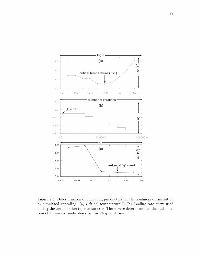
� The value of T which corresponds to the minimum Eav estimates the critical

temperature, Tc (Figure 2.1a).

Having found Tc I can proceed to �x the cooling rate. The initial temperature

is high (T = 10 in my inversions). This value is chosen based on the estimate of

Tc. My experimental runs have shown that for convergence to a global minimum,

one needs to start with a initial value of T at least two orders of magnitude greater

than the critical temperature, Tc. The only e�ect of choosing a higher initial

temperature will be that it takes a larger number of iterations for the optimization

to convergence to the same solution.

The high initial temperature destroys any order in the initial model, guarantee-

ing that it will not bias the inversion. Within a few thousand iterations I rapidly

20

decrease T to the critical temperature. On reaching Tc, I slow the rate of decrease

of T , enabling the optimization process to settle in the deepest minimum. Figure

2.1b shows a typical cooling rate curve. Here, I keep the temperature constant at

Tc from the 2000th to the 50,000th iteration, and then decrease it at a very slow

rate. After trial runs I found this technique to e�ect the fastest convergence, of

those that I tried. Other attempts, like linearly reducing the temperature with

iteration, caused the algorithm to get trapped in a local minimum.

To determine the other empirical parameter, q I do the following:

� At the critical temperature, Tc, compute the average least-square error, Eav

for a short run of the optimization process.

� Repeat the above step for each of a suite of q values.

� The value of q that corresponds to the minimum Eav will give the optimum

convergence (Figure 2.1c).

In summary, the nonlinear optimization scheme does not involve any matrix

computations, and requires only repeated forward modeling. The former condi-

tion makes it immune to problems of matrix singularity and instability, for example

those due to ill-conditioned matrices and small eigenvalues. The memory require-

ments are manageable since during each iteration only the values of all the model

parameters need to be stored. For the model sizes I use during the course of my

work (between 600 and 4000 model parameters), the optimization required between

12 to 48 hours of computation time on a SPARCstation 2. The need to do repeated

21

forward modeling makes the method computationally expensive when the number

of model parameters increases, and optimization speed critically depends on the

speed of the forward-modeling process. At the same time, the reliance only on

forward modeling facilitates simultaneous optimization of di�erent types of data.

The annealing parameters are determined empirically before proceeding to op-

timize for every problem. In this section we saw that the acceptance probability of

new models has a distribution similar to the posterior probability of model param-

eters in the nonlinear least-squares formulation. This justi�es using the models

obtained during the optimization in a statistical analysis to determine the uncer-

tainties associated with the �nal model parameters.

2.4 Pre-stack Migration

To image structures in regions where velocity undergoes rapid lateral changes, one

needs to employ pre-stack migration. Pre-stack migration directly images re ec-

tive structure from re ections in multi-o�set seismic record sections, bypassing the

NMO correction and stacking procedure used in standard seismic survey processing

(Jain and Wren, 1980; Schultz and Sherwood, 1980). Unlike NMO correction and

stacking, pre-stack migration is not limited in applicability to regions having only

gently-dipping re ectors (Claerbout, 1985, p. 188). In this section I brie y explain

the underlying principles of the pre-stack migration technique used to image struc-

tures (re ectors) through velocities obtained after the non-linear optimization of

22

critical temperature ( Tc )

T = Tc

value of "q" used

E a

v

log T

number of iterations

qE

av

log

T

(a)

(b)

(c)

(s )

(s )

22

Figure 2.1: Determination of annealing parameters for the nonlinear optimizationby simulated-annealing. (a) Critical temperature Tc (b) Cooling rate curve usedduring the optimization (c) q parameter. These were determined for the optimiza-tion of three-box model described in Chapter 4 (see 4.4.1)

23

travel times.

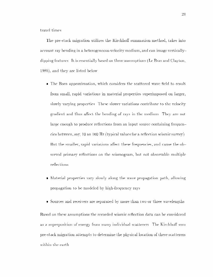
The pre-stack migration utilizes the Kirchho� summation method, takes into

account ray bending in a heterogeneous-velocity medium, and can image vertically-

dipping features. It is essentially based on three assumptions (Le Bras and Clayton,

1988), and they are listed below.

� The Born approximation, which considers the scattered wave �eld to result

from small, rapid variations in material properties superimposed on larger,

slowly varying properties. These slower variations contribute to the velocity

gradient and thus a�ect the bending of rays in the medium. They are not

large enough to produce re ections from an input source containing frequen-

cies between, say, 10 an 100 Hz (typical values for a re ection seismic survey).

But the smaller, rapid variations a�ect these frequencies, and cause the ob-

served primary re ections on the seismogram, but not observable multiple

re ections.

� Material properties vary slowly along the wave propagation path, allowing

propagation to be modeled by high-frequency rays.

� Sources and receivers are separated by more than two or three wavelengths.

Based on these assumptions the recorded seismic re ection data can be considered

as a superposition of energy from many individual scatterers. The Kirchho� sum

pre-stack migration attempts to determine the physical location of these scatterers

within the earth.

24

I follow the procedure of Louie et al. (1988) to implement the pre-stack mi-

gration described above. The objective is to map the recorded seismic traces

into a depth section by computing the travel time from the source to the depth

point and back to the receiver, assuming the velocity distribution in the medium

is known. The �rst step is to compute travel times through the medium from

each possible source and receiver point. I use an e�cient travel-time calculator

for two-dimensional models (Vidale, 1988) based on a �nite-di�erence solution to

the eikonal equation. This accounts for turning rays, thus enabling imaging of

structures having dips greater than 900. Assuming every point in the model may

be a scatterer, the algorithm computes and adds up the total two-way re ection

time from every possible re ection depth point to each source-receiver pair.

The next step is to obtain the amplitude corresponding to this travel time from

the seismogram recorded by the appropriate source-receiver pair. This amplitude

is summed into the model (migrated section) at that depth point. Each individual

travel time calculation for each trace could include many points of re ection along

a three-dimensional projection of an ellipsoid. The tomographic summation of all

traces at a particular calculated time will allow for the de�nition of a unique point

in the earth for all ellipses calculated for each individual source-receiver pair (Louie

and Qin, 1989). Coherent and continuous events at that time will constructively

interfere, indicating the presence of earth structure in the migrated section.

This chapter describes the three methods often used during the course of my

thesis work. I show in the subsequent chapters that the linear method is initial-

25

model dependent and thus will �nd the global minimum only when the starting

model is close to the expected solution. The nonlinear method is shown to be very

robust. It is able to recover similar solutions while starting out with very di�erent

models. It reconstructs reasonable models with minimum a priori constraints.

It performs much more robustly than any inversion scheme when the problem is

severely under-determined. I successfully apply it to optimize di�erent data types

� refractions, re ections, and the coherency of re ected arrivals.

The pre-stack migration operates in the shot-receiver space, the same domain

in which the data are collected. Accurate migration is possible because the opti-

mizations give us good control on lateral velocity variations, barring which, one

would have to transform the data to a midpoint-o�set space (Claerbout, 1985)

to avoid migration errors. The advantage of staying in the shot-receiver space is

that it helps preserve the accuracy of both re ector dip and ray propagation angle.

Moreover it avoids spatial aliasing when the shot spacing is large.

26

Chapter 3

Velocity Estimation and Imaging by Optimization of

First-Arrival Times

3.1 Abstract

In this chapter, I document the application of a Monte Carlo-based optimization

scheme called generalized simulated annealing to invert �rst-arrival times for ve-

locities. The input are \dense" common depth point (CDP) data having high

multiplicity, as opposed to traditional refraction surveys with few shots. A fast

�nite-di�erence solution of the eikonal equation computes �rst arrival travel times

through the velocity models. I test the performance of this optimization scheme

on synthetic models and compare it with a linearized inversion. The tests indi-

cate that unlike the linear methods, the convergence of the simulated-annealing

algorithm is independent of the initial model. In addition, this scheme produces a

suite of \�nal" models having comparable least-square error. These allow one to

choose a velocity model most in agreement with geological or other data. Exploit-

ing this method's extensive sampling of the model space, one can determine the

uncertainties associated with the velocities.

27

I use the optimization procedure on �rst-arrival times picked from three sets of

�eld shot records. The �rst data set comes from COCORP Death Valley Line 9,

which traverses the central Basin and Range province in California and Nevada.

The second data set is marine re ection data collected by the EDGE consortium

across the Hosgri fault, o�shore California. Shot gathers recorded along COCORP

Mojave Line 1 form the third data set. This line crosses the Mojave segment of

the San Andreas fault. In all three cases the velocities in the region undergo rapid

lateral changes, and this technique images these variations with little a priori

information. For the last two data sets, I also demonstrate how one can image

the fault plane itself using the accurate velocities obtained by the optimization

procedure.

Lastly, in all the above cases, I compare the results with prior studies in the

regions. I brie y discuss the tectonic implications of the velocity models and fault

images obtained by my methods in each of the three areas.

3.2 Introduction

I use �rst arrivals, including both direct and refracted phases recorded during

surface seismic surveys, to obtain shallow velocity structure. By doing so, one

exploits the increasing multiplicity of \refraction" surveys. Whereas early surveys

were simply shot-reversed, we now have common depth point data with many

shots and high multiplicity. This enables us to obtain high-resolution images of

28

the shallow subsurface.

Determination of near-surface velocities is important for geological, geophysical,

and engineering studies. The e�ect of the low-velocity weathering layer has to be

accounted for in engineering site investigations (e.g.: Hatherly and Neville, 1986).

Lateral velocity variations in this layer contaminate stacked seismic sections and

introduce apparent structure on deeper re ection events. These are removed by

\statics" corrections, which need accurate velocity estimates (Farrell and Euwema,

1984; Russell, 1989). Shallow velocity structure determined from refraction times

have been used for ground water studies (e.g.: Haeni, 1986). In addition, imaging

near-surface crustal structure is important in neotectonic studies of some regions

(e.g.: Geist and Brocher, 1987).

Various schemes are employed to determine refraction velocities. Layered ve-

locity models can be obtained using, for example, the Herglotz-Wiechert formula

(Gerver and Markushevitch, 1966), wavefront methods (Thornburgh, 1930; Rock-

well, 1967), or the plus-minus method (Hagedoorn, 1959). Palmer (1981) and Jones

and Jovanovich (1985) describe methods to derive the depth to an irregular refrac-

tor as well as lateral velocity changes along the refractor. Clayton and McMechan

(1981) and McMechan et. al. (1982) use a wave �eld transformation approach,

that avoids preprocessing of the data, to invert refraction data for a velocity pro-

�le. Several workers, for example, Hampson and Russell (1984), de Amorim et al.

(1987), Olsen (1989), Docherty (1992), and Simmons and Backus (1992) employ

linearized inversion schemes to invert �rst-arrival times for near-surface velocities.

29

Travel time inversion is a nonlinear process because a perturbation in the velocity

�eld results in changes in the ray paths through it. Linearized inversions involve

local linearization of this nonlinear problem. This makes them initial-model depen-

dent, and a poor choice of the starting model could cause the inversion to converge

to an incorrect solution at a local minimum.

To circumvent this problem, I demonstrate the use of a nonlinear optimization

technique, namely a generalized simulated annealing, to invert �rst-arrival times

for shallow velocities. I rapidly compute travel times through models by a method

avoiding ray tracing. It employs a fast �nite-di�erence scheme based on a solution

to the eikonal equation (Vidale, 1988). This accounts for curved rays and all

types of primary arrivals, be they direct arrivals, refractions, or di�ractions. I test

the optimization process on synthetic models that mimic typical geological cross-

sections encountered in the �eld and compare its performance with a linearized

inversion and demonstrate the initial-model dependence of the latter.

Velocities obtained from refraction studies �nd wide use in statics corrections

(i.e., to remove near-surface e�ects interfering with deeper re ections). To test the

utility of our method for statics correction I compute vertical travel times through

the models obtained. This also serves to compare the robustness of the inversion

results using the di�erent methods. Another advantage of the simulated-annealing

algorithm is that it produces a suite of �nal models having comparable least-square

error. This enables one to choose models most likely to represent the geology of a

region. One can also use this property to determine the uncertainties associated

30

with the model velocities obtained.

I use this technique on three di�erent data sets to obtain velocity information

of the crust at relatively shallow horizons. The �rst data set is COCORP Death

Valley line 9, which traverses the central Basin and Range province. Accurate

velocity models in this region are necessary to test models that can explain the

observed extreme crustal extension. The second data set is shot gathers recorded by

the EDGE consortium across the Hosgri fault (RU-3 line), o�shore California. Use

of the nonlinear optimization technique obtains a high-resolution velocity structure

in this region, with minimum a priori constraints. The third data set is from the

COCORP Mojave line 1, part which crosses the San Andreas fault in southern

California. The only constraints that go into our method are the size of the model

and the minimum and maximum crustal velocities one is likely to encounter in the

region. I then use the velocity results in pre-stack Kirchho�-sum migrations that

account for curved rays, to accurately image the Hosgri and San Andreas faults.

3.3 Results From Synthetic Models

First, I test our optimization scheme using synthetic models and compare its per-

formance against a linearized inversion scheme that also employs curved rays. The

linearized method is described in chapter 2. The synthetic models correspond

to velocity distributions one might encounter in the �eld: a low-velocity basin

model (Figure 3.1a), a high-velocity intrusion model (Figure 3.5a) and a low-

31

velocity layer model (Figure 3.8a). The models are 40 km long and 8 km deep

with a grid size of 1 km. There is a source at every other grid point (for a total of

20 sources). The �rst arrivals from each source are recorded at 40 receivers along

the surface, resulting in 800 total observations.

3.3.1 Low-velocity basin

Figure 3.1a shows a velocity model of an asymmetric basin. The velocity within

the basin increases from 4 km/s to 5 km/s. This is underlain by a high-velocity (6

km/s) layer. A fault-like displacement is incorporated along the right wall of the

basin.

During the nonlinear optimization the velocity is allowed to vary between 1.5

km/s and 8.3 km/s. I perform two sets of annealing optimization; one starting

with a constant velocity model at 3 km/s, and the other with a velocity of 8 km/s.

The results are shown in Figures 3.1b and 3.1c. The cooling rate is determined

separately for each of these optimization runs. The critical temperature, Tc is 0.001

for both runs (Figure 3.1a). For illustration I show the least-square error variation

for the �rst run (initial velocity of 3 km/s) in Figure 3.1c. The error decreases

from 3.25 s2 for the constant velocity �eld to 0.006 s2 for the �nal accepted model.

The �nal accepted models obtained after both the optimization runs (Figure

3.2b, c) look quite similar, showing that convergence of the generalized simulated-

annealing is independent of the initial model. The random perturbations performed

32

40

de

pth

, km

-8-6-4-20

de

pth

, km

0 10 20 30

-8-6-4-20

de

pth

, km

-8-6-4-20

sources and receivers

(a) true

(b) anneal : 3 km/s

(c) anneal : 8 km/s

3.5 4.0 4.5 5.0 5.5 6.0 ve

l, km/s

vel, km

/sve

l, km/s

3.5 4.0 4.5 5.0 5.5 6.0

0 10 20 30 40offset, km

4 6 81012

(d) svd : 3 km/s

(e) svd : 8 km/s

(f) svd : 8 km/s

3.5 4.0 4.5 5.0 5.5 6.0 ve

l, km/s

3.5 4.0 4.5 5.0 5.5 6.0 ve

l, km/s

3.5 4.0 4.5 5.0 5.5 6.0 ve

l, km/s

-8-6-4-20

de

pth

, km

-8-6-4-20

de

pth

, km

-8-6-4-20

de

pth

, km

Figure 3.1: Generalized simulated annealing optimization and linearized inversionresults for the low-velocity basin model. (a) The true model with 20 sourcesand 40 receivers along the top. (b) and (c) show the annealing results startingwith a constant velocity of 3 km/s and 8 km/s respectively. (d) and (e) show theresults of a linearized inversion scheme, employing a singular-value decompositionto invert the matrix, with two di�erent initial models. (f) Un-scaled version of(e) showing the anomalous high velocity reconstruction in the lower right. Thevelocity scale shown on the right of (d) and (e) also applies to (a), (b), and (c).

33

2

critical temperature (Tc)

log-log

linear-log

linear-log

Tc

( a )

( b )

( c )

log (temperature)

iteration number

iteration number

log

(L2

err

or)

(s

)2lo

g(L

2 e

rro

r) (

s )2

-6.0 -4.0 -2.0 0.0 2.0

-0.5

0.0

0.5

1.0

log

(L2

err

or)

(s

)2

Figure 3.2: Determination of annealing parameters for the optimization of thelow-velocity basin model. (a) Critical temperature Tc. (b) Cooling rate curveused. (c) Least-square error variation during the optimization.

34

during annealing destroy any \order" or bias present in the initial model. The

optimization does not recover the exact shape of the basin, but it images the basin

bottom well. It recovers the velocities within the basin but fails to image the sharp

transition between the 4 km/s layer and the 5 km/s layer. The optimization poorly

reconstructs the top 3.5 km/s velocity layer.

In addition, a spurious low-velocity zone is present at the lower right edge

of the image. Lack of ray coverage in this region is the cause for the anomaly.

The \hitcount" is computed (number of rays that sample a particular cell) plot

(Figure 3.3c) by tracing rays through the medium. I achieve this by invoking

the principle of seismic reciprocity and adding together the source-receiver and

receiver-source times, then following the minimumtime path according to Fermat's

principle (Pullammanappallil and Louie, 1993).

The generalized annealing optimization produces a suite of models which have

comparable least-square error near the global minimum. One can use known infor-

mation about the region to choose the �nal model. During the optimization pro-

cess, the method tries out numerous models (in our case the number was 200,000).

Thus it samples a large area of the model space, and I make use of this to de-

termine the uncertainties associated with the �nal model parameters. I perform

a statistical analysis on all the trial models and normalize the deviations with re-

spect to the �nal accepted model (Figure 3.3b). The deviations range from 5 %

to 35 %. The well-constrained regions are resolved to within 0.3 - 0.5 km/s. As

expected, the regions with poor ray coverage have a higher deviation associated

35

with them. Figure 3.3a shows the model obtained by averaging over 36 models

with similar least-square error near the global minimum. Models from each of the

three di�erent runs, having an initial velocity of 3, 5, and 8 km/s, are used in this

averaging. This process enables us to smooth the e�ects of random perturbations

that might be present in the �nal model.

Figures 3.1d and 3.1e show the inversion results using the linearized scheme,

starting with constant velocities of 3 km/s and 8 km/s, respectively. The inversion

that started with a velocity of 8 km/s does a better job of reconstructing the basin

shape and depth. Like the nonlinear optimization, it fails to recover the uppermost

low-velocity layer. But unlike annealing, the velocity models obtained after the

two runs are not identical, illustrating the initial-model dependence of linearized

inversion. I explore this further in the other synthetic tests. I show an un-scaled

version of the result in Figure 3.1f to demonstrate that, like the optimization

scheme, the linearized inversion reconstructs an anomalous zone (in this case with

high velocity) in the poorly-constrained lower right corner of the image.

It is standard practice to use the velocity information obtained from �rst-arrival

times to perform \statics" corrections. These involve removing the delay e�ects of

near-surface layers on deeper re ections or refractions. It requires accurate esti-

mation of vertical travel times through inverted models. Performing this exercise

also allows me to test the robustness of the models obtained from di�erent inver-

sion runs. Vertical travel time curves computed through the di�erent models are

shown in Figure 3.4. The times from both annealing results are identical, and

36

-8-6-4-20

de

pth

, km

3.5 4.0 4.5 5.0 5.5 6.0 ve

l, km/s

0 10 20 30 40offset, km

-8-6-4-20

de

pth

, km

0

2

4 cou

nt

(a) average model

(c) hitcount

-8-6-4-20

de

pth

, km

102030

% n

orm

. de

v

(b) norm. std. deviations

Figure 3.3: (a) Average of the \�nal" low-velocity basin models, with compa-rable least-square error. (b) The standard deviation, normalized with respect tothe �nal accepted-model, associated with the obtained model parameters. (c) Ahitcount plot through the true model for all source-receiver pairs. The regions withno ray coverage are poorly constrained.

37

diverge from the true times near the model edges. The presence of the spurious

low-velocity zone near the lower right corner probably causes this di�erence at the

edges. The times through the linearized models are not identical, and di�er by as

much as 0.5 seconds at some nodes. This suggests that the models obtained by

the nonlinear optimization scheme are more robust, even though the least-square

error through the �nal model obtained after the linearized scheme is smaller 0.003

s2.

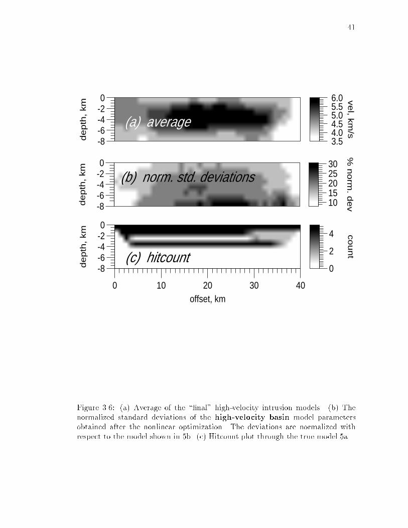
3.3.2 High-velocity intrusion

A high-velocity body (like an intrusion) beneath low-velocity sediments at shal-

low depths is another geological feature likely to be encountered in the �eld. To

examine the e�ectiveness of the inversions in reconstructing such features from

�rst-arrival times, I construct the model shown in Figure 3.5a. A 6 km/s body is

embedded in a 5 km/s layer. The maximum velocity in the model is also 6 km/s.

As in the previous example, I perform two di�erent nonlinear optimizations

- one with an initial velocity of 3 km/s and another with a velocity of 5 km/s.

Figures 3.5b and 3.5c show the results, and as before, the �nal models from the

two runs look similar. The annealing process seems to smear out the high velocity

zone, and it fails to recover the top low-velocity layer. The region beneath the

high-velocity body is unconstrained, due to lack of ray coverage (Figure 3.6c).

Consequently there is poor reconstruction of velocities there. To determine the

uncertainties associated with the model parameters I perform a statistical analysis

38

offset, km

verti

cal t

rave

ltimes

, s

true model

anneal: 3 km/s , 8 km/s

svd: 3 km/s

svd: 8 km/s

Figure 3.4: Vertical travel times through the �nal low-velocity basin models,obtained from the di�erent runs, calculated at each node along the surface. Sincemodels from �rst-arrival information are often used for \statics" corrections, thistests the robustness of the inversion.

39

along the lines described in the previous section. The normalized deviations (with

respect to the �nal accepted velocity model; Figure 3.6b) vary between 8 - 30 %, the

higher deviations being associated with regions of poor ray coverage (comparing

Figure 3.6b with 3.6c). Interestingly, taking an average of all the models used

in the statistical analysis (Figure 3.6a) seems to have recovered the shape of the

high-velocity body very well. This is potential advantage of using the simulated-

annealing algorithm. One can cancel the random perturbations not common to all

the models having comparable least-square error.

Figures 3.5d and 3.5e show the results of the linearized inversion with starting

models of 3 km/s and 5 km/s, respectively. The two results look very di�erent,

demonstrating the strong initial-model dependence of the linear scheme. The in-

version with an initial velocity of 5 km/s does a better job of reconstructing the

velocities. The high-velocity zone is again smeared out and the region below it is

poorly imaged.

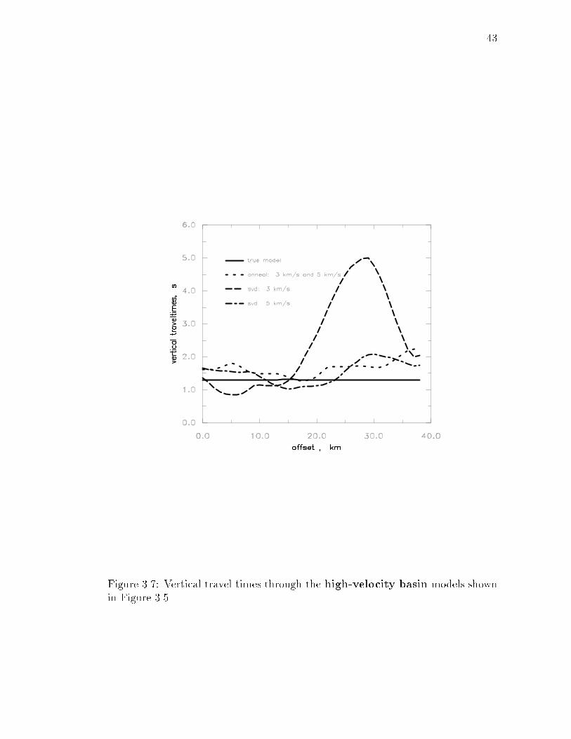
Once again I calculate vertical travel times through the models (rays traveling

from the bottom to the top). From Figure 3.7 one can see that these times ob-

tained by the optimization diverge from the true times by 0.5 second or less. The

linearized inversion result starting with a velocity of 3 km/s has times diverging

by as much as 4 seconds near the right edge. Moreover, the linearized inversion

results yield di�erent vertical times, indicating that they are not very robust.

40

3.5 4.0 4.5 5.0 5.5 6.0 ve

l, km/s

-8-6-4-20

de

pth

, km

(a) true

(b) anneal: 3 km/s

(c) anneal: 5 km/s

(d) svd: 3 km/s

0 10 20 30 40offset, km

(e) svd: 5 km/s

-8-6-4-20

de

pth

, km

-8-6-4-20

de

pth

, km

-8-6-4-20

de

pth

, km

-8-6-4-20

de

pth

, km

Figure 3.5: Nonlinear optimization and linearized inversion results for the high-velocity basin model. (a) The true model. (b) and (c) show the optimizationresults. (d) and (e) show the results from a linearized inversion scheme. Theconstant velocities of the initial models are indicated. The velocity scale shown onthe right of (a) applies to all the panels.

41

-8-6-4-20

de

pth

, km

1015202530

% n

orm

. de

v

-8-6-4-20

de

pth

, km

3.5 4.0 4.5 5.0 5.5 6.0 v

el, k

m/s

(a) average

0 10 20 30 40offset, km

-8-6-4-20

de

pth

, km

0

2

4 co

un

t

(b) norm. std. deviations

(c) hitcount

Figure 3.6: (a) Average of the \�nal" high-velocity intrusion models. (b) Thenormalized standard deviations of the high-velocity basin model parametersobtained after the nonlinear optimization. The deviations are normalized withrespect to the model shown in 5b. (c) Hitcount plot through the true model 5a.

42

3.3.3 Low-velocity layer model

The third model I use in synthetic tests is one with a low-velocity layer of 3.0 km/s

(Figure 3.8a). The low-velocity layer is bounded by higher velocities above and

below. The maximum velocity is again 6 km/s at the bottom. The ray coverage

through the model (not shown), indicates that none of the rays travel along the

low-velocity layer. The optimization results for two di�erent starting models, 3

km/s and 8 km/s, are shown in Figures 3.8b and 3.8c. The two results again look

very similar. They do not image the low-velocity layer, instead reconstructing

velocities that smoothly increase with depth. In the statistical analysis I use all

trial models. The normalized deviations (Figure 3.8f) vary from 1 % to 18 %.

There are regions in the model that have low deviation though their ray cov-

erage is poor. This is because these regions are not perturbed during annealing,

since my statistical analysis includes all the trial models. It also indicates that it

is impractical to sample the model space well enough to obtain appropriate devi-

ations in all poorly-constrained parts of the model. Thus a low deviation could

sometimes be misleading. Obviously, one should only believe deviation values from

nodes having non-zero hitcount.

The linearized inversion results shown in Figure 3.8d and 3.8e also fail to recon-

struct the low-velocity layer. The vertical times through the annealing results (not

shown) are very similar, di�ering from the true times by only 0.2 seconds. The

linearized inversion results show di�erent vertical times, and they diverge from the

43

Figure 3.7: Vertical travel times through the high-velocity basin models shownin Figure 3.5

44

true times by as much as 2 seconds near the edges. These results demonstrate

that simulated-annealing optimization produces more robust models, that are not

dependent on the initial model. These advantages hold even for models such as

the low-velocity layer that surface travel-time data cannot constrain.

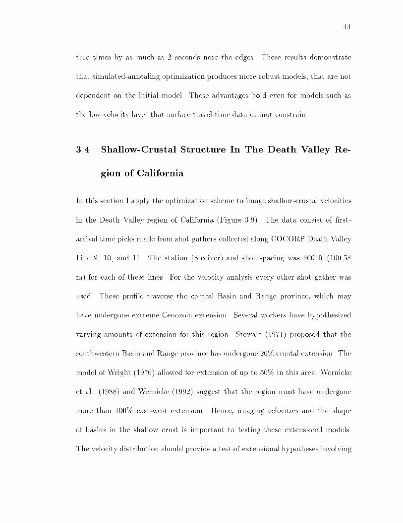
3.4 Shallow-Crustal Structure In The Death Valley Re-

gion of California

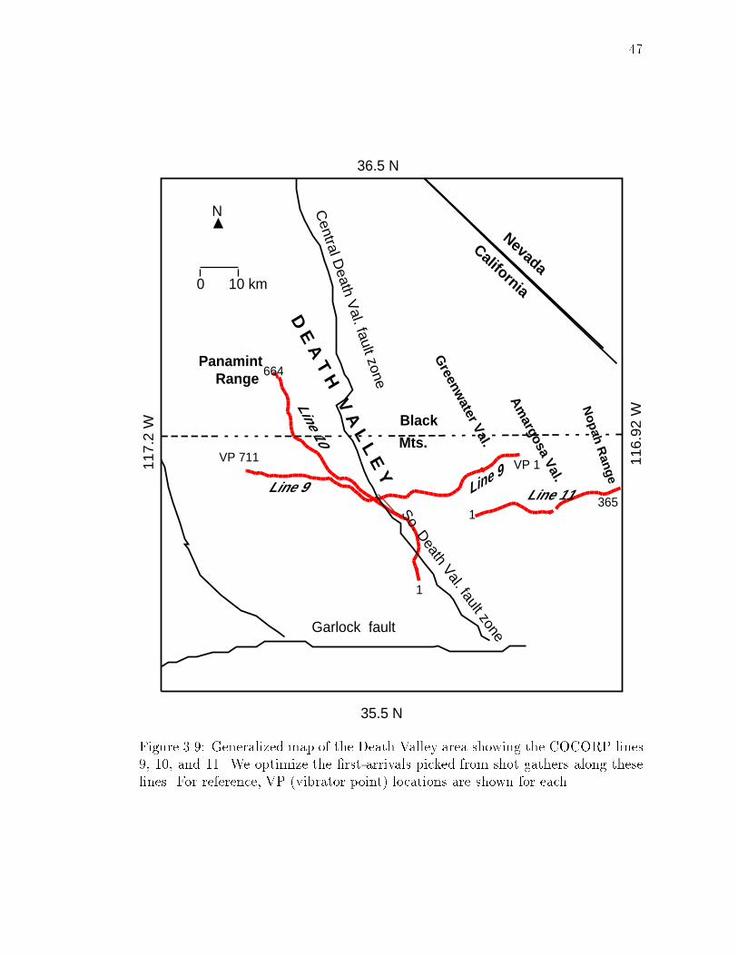
In this section I apply the optimization scheme to image shallow-crustal velocities

in the Death Valley region of California (Figure 3.9). The data consist of �rst-

arrival time picks made from shot gathers collected along COCORP Death Valley

Line 9, 10, and 11. The station (receiver) and shot spacing was 300 ft (100.58

m) for each of these lines. For the velocity analysis every other shot gather was

used. These pro�le traverse the central Basin and Range province, which may

have undergone extreme Cenozoic extension. Several workers have hypothesized

varying amounts of extension for this region. Stewart (1971) proposed that the

southwestern Basin and Range province has undergone 20% crustal extension. The

model of Wright (1976) allowed for extension of up to 50% in this area. Wernicke

et al. (1988) and Wernicke (1992) suggest that the region must have undergone

more than 100% east-west extension. Hence, imaging velocities and the shape

of basins in the shallow crust is important to testing these extensional models.

The velocity distribution should provide a test of extensional hypotheses involving

45

6

-8-6-4-20

de

pth

, km (a) true

4

5

vel, km

/s

3

-8-6-4-20

de

pth

, km (b) anneal: 3 km/s

4

5

6 vel, km

/s

3

4

5

6 vel, km

/s

-8-6-4-20

de

pth

, km (c) anneal: 8 km/s

3

(d) svd: 3 km/s4

5

6 vel, km

/s

3-8-6-4-20

de

pth

, km

3

4

5

6 vel, km

/s

(e) svd: 8 km/s

-8-6-4-20

de

pth

, km

0 10 20 30 40offset, km

-8-6-4-20

de

pth

, km

51015

% n

orm

. de

v

(f) percent deviations

Figure 3.8: Results from performing annealing optimization and a linearized in-version on the low-velocity layer model shown in (a). The velocities used in thestarting model are indicated. (f) shows the deviations of the velocities obtainedby annealing (b, c). The velocity scale on the right side of (d) and (e) also appliesto (a), (b), and (c).

46

large vertical movements or alterations of the shallow crust. Pullammanappallil

et al. (1994), combine these results with information from deeper crust obtained

from surface-wave analysis. They conclude that extension in this region must have

happened by a mechanism that did not involve signi�cant alterations in upper and

mid-crustal velocities.

3.4.1 Velocity Estimation Using COCORP DV Line 9 Data

Line 9 traverses from the Amargosa River in the east to the Panamint Mountains

in the west (Figure 3.9) and cuts across several alluvial valleys. I use a total of

6213 �rst-arrival times picked from 281 shot gathers. To overcome the e�ect of

bends in the pro�le, I project the source locations to a line while maintaining the

true o�sets of the source-receiver pairs. Thus the velocities obtained after the

optimization will show some lateral smearing. Due to this projection, the shot

spacing was not uniform along the entire length of the line. It varies between 40 m

and 1.8 km with an average shot-spacing of 190 m. The maximum source-receiver

o�set of the survey is 10 km.

For the optimizations I use a model that is 62 km long and 5 km deep, with a

grid spacing of 500 m. There is signi�cant topography along the pro�le. I include

elevation information by extrapolating the times to sources and receivers not on

grid points. For this I assume plane-wave incidence at the receivers. The initial

model has a constant velocity of 2 km/s. Velocity is allowed to vary between 1.5

and 8 km/s during the annealing procedure. I �x the empirical annealing constants

47

365

664

1

1

NevadaCalifornia

Garlock fault

Central D

eath Val. fault zone

So. Death Val. fault zone

PanamintRange

Black

Mts.D

E A T H V A L L E Y

Line 9Line 9

VP 711VP 1 1

16

.92

W

11

7.2

W

35.5 N

36.5 N

N

Greenw

ater Val.

0 10 km

Line 11

Line 10

Amargosa Val.

Nopah R

ange

Figure 3.9: Generalized map of the Death Valley area showing the COCORP lines9, 10, and 11. We optimize the �rst-arrivals picked from shot gathers along theselines. For reference, VP (vibrator point) locations are shown for each.

48

by performing a series of short runs as described in Chapter 2. In this case I found

the critical temperature to be 0.01.

Figure 3.10a shows the result of the optimization. The least-square error went

from 1.51 s2 for the constant velocity model to 0.007 s2 for the �nal model. The

low-velocity regions in the �nal model are associated with alluvial basins while

the shallow high velocities show the basement rocks below mountain ranges. The

prominent basin around VP 450 - 525 corresponds to central Death Valley. The

Black Mountains and the Panamint Range have relatively higher velocities (4.5 -

5 km/s) beneath them.

These velocities compare very well with the forward modeling results of Geist

and Brocher (1987). As in the case of the synthetic examples, I obtain the model

velocity uncertainties. The deviations range from 0 to 45% of the average model

(Figure 3.10c). Figure 3.10b shows the average model obtained from 20 models

having similar least-square error as the �nal model. I plot the hitcount of the rays

through the �nal model in Figure 3.10d to allow us to see that the regions with

higher deviation also have poor ray coverage.

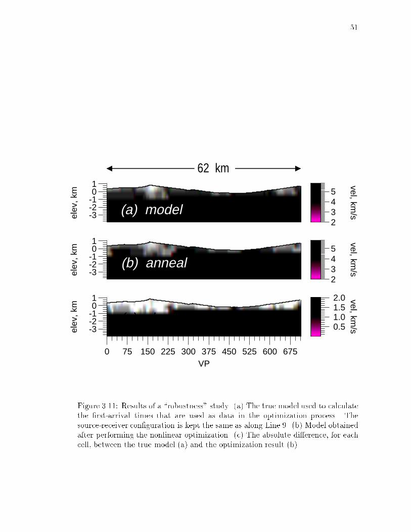
How do the deviations obtained relate to the actual di�erence between the

\true" model and the optimization result? Are the normalized deviations a good

measure of the resolution of the model parameters? To answer these questions

I perform a \robustness" study. For this, I use travel times computed through

a model resembling the optimization result (Figure 3.11a) as \data." I keep the

source-receiver con�guration the same as the actual survey and take into account

49

the elevation corrections. As for the data optimization, the starting velocity is

constant (equal to 2 km/s) and is allowed to vary between 1.5 and 8 km/s.

Figure 3.11b shows the reconstructed model. The absolute di�erence between

the reconstructed model and the true model is shown in Figure 3.11c. The maxi-

mum error of 2 km/s is in a region of no ray coverage (Figure 3.11c). The error in

recovering the low-velocity basin is about 0.5 km/s while all the other regions with

ray coverage are imaged to within 0.2 km/s of the true model. Next, I compute

both the uncertainties and the normalized deviations associated with the model

parameters (Figure 3.12a) by our statistical analysis. Figure 3.12b shows normal-

ized deviations obtained by dividing the absolute di�erence (Figure 3.11c) by the

average model of the velocity models used in our statistical analysis. Comparing

Figure 3.12a and 3.12b, one can see that the normalized deviations are indeed a

measure of the uncertainties associated with the �nal model parameters. They

give us the upper bound to the uncertainties, if not the exact error.

3.4.2 Velocity Estimates Under COCORP DV Line 10

The pro�le of line 10 extends from the southern end of the Nopah Range in the east

to the southern part of the Black Mountains in the west (Figure 3.9). I use 4004

travel time picks from 114 shot gathers as input to the optimization process. The

shot-spacing along the projected line ranges from 70 m to 1.7 km. The velocity

model is 34 km long 4 km deep, with a grid spacing of 500 m. Again, I start with

a constant velocity model (2 km/s) and obtain the result in Figure 3.13a. The

50

-3-2-10

1

elev

, km

345

vel, km/s

-3-2-10

1

elev

, km

345

vel, km/s

-3-2-10

1

elev

, km

10 20 30 40 %

dev

0 75 150 225 300 375 450 525 600 675VP

-3-2-10

1

elev

, km

0

2

4 count

(a) anneal

(b) average

(c) norm. st. dev.

(d) hitcount

unconstrained

death valleyblack mtnsgreenwater val panamint mtns

62 km

East West

Figure 3.10: (a) Result of the nonlinear �rst-arrival optimization along COCORPDeath Valley Line 9. The major physiographic features are also indicated (seeFigure 11). (b) Model obtained by averaging the velocity models used in ourstatistical analysis. (c) Deviations in the obtained model parameters normalizedwith respect to the average model shown in (b). (d) Ray coverage diagram throughthe model in (a) showing regions of poor coverage.

51

-3-2-10

1

elev

, km

2345

vel, km/s

-3-2-10

1

elev

, km

2345

vel, km/s

0 75 150 225 300 375 450 525 600 675VP

-3-2-10

1

elev

, km

0.5 1.0 1.5 2.0 vel, km

/s

62 km

(a) model

(b) anneal

(c) abs. diff.

Figure 3.11: Results of a \robustness" study. (a) The true model used to calculatethe �rst-arrival times that are used as data in the optimization process. Thesource-receiver con�guration is kept the same as along Line 9. (b) Model obtainedafter performing the nonlinear optimization. (c) The absolute di�erence, for eachcell, between the true model (a) and the optimization result (b).

52

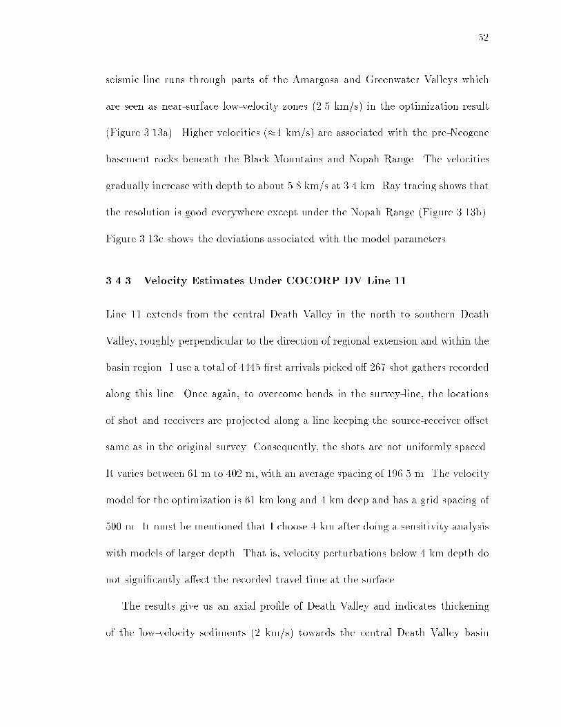
seismic line runs through parts of the Amargosa and Greenwater Valleys which

are seen as near-surface low-velocity zones (2.5 km/s) in the optimization result

(Figure 3.13a). Higher velocities (�4 km/s) are associated with the pre-Neogene

basement rocks beneath the Black Mountains and Nopah Range. The velocities

gradually increase with depth to about 5.8 km/s at 3.4 km. Ray tracing shows that

the resolution is good everywhere except under the Nopah Range (Figure 3.13b).

Figure 3.13c shows the deviations associated with the model parameters.

3.4.3 Velocity Estimates Under COCORP DV Line 11

Line 11 extends from the central Death Valley in the north to southern Death

Valley, roughly perpendicular to the direction of regional extension and within the

basin region. I use a total of 4445 �rst arrivals picked o� 267 shot gathers recorded

along this line. Once again, to overcome bends in the survey-line, the locations

of shot and receivers are projected along a line keeping the source-receiver o�set

same as in the original survey. Consequently, the shots are not uniformly spaced.

It varies between 61 m to 402 m, with an average spacing of 196.5 m. The velocity

model for the optimization is 61 km long and 4 km deep and has a grid spacing of

500 m. It must be mentioned that I choose 4 km after doing a sensitivity analysis

with models of larger depth. That is, velocity perturbations below 4 km depth do

not signi�cantly a�ect the recorded travel time at the surface.

The results give us an axial pro�le of Death Valley and indicates thickening

of the low-velocity sediments (2 km/s) towards the central Death Valley basin

53

-3-2-10

1

dept

h, k

m

20 25 30 35 40 %

dev

-3-2-10

1

dept

h, k

m

15 20 25 30 35 40 %

dev

0 75 150 225 300 375 450 525 600 675VP

-3-2-10

1

dept

h, k

m

0

2

4 count

(a) norm. std. deviations

(b) norm. abs. diff.

(c) hitcount

62 km

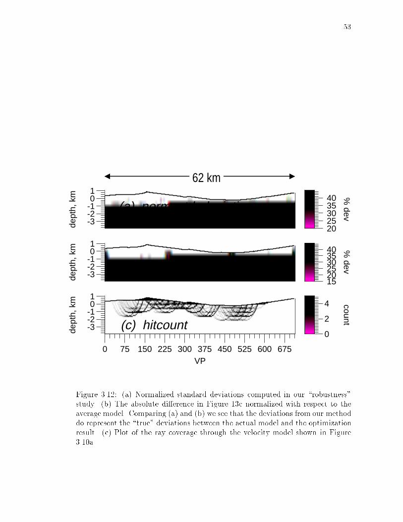
Figure 3.12: (a) Normalized standard deviations computed in our \robustness"study. (b) The absolute di�erence in Figure 13c normalized with respect to theaverage model. Comparing (a) and (b) we see that the deviations from our methoddo represent the \true" deviations between the actual model and the optimizationresult. (c) Plot of the ray coverage through the velocity model shown in Figure3.10a.

54

34 km

-3-2-10

Ele

v.,

km

345

Ve

l., km

/s

Black Mts.Greenwater Valley Nopah Range

(a) Line 10: velocity

W E

1 50 100 150 200 250 300 350

-3-2-10

Ele

v.,

km

0.5 1.5 2.5 3.5 4.5 %

De

v.

(b) Line 10: norm. std. dev.W E

VP

50 100 150 200 250 300 350

-3-2-10

0

2

4

6

co

un

t

1

Ele

v.,

km

(c) Line 10: Hitcount

34 km

Figure 3.13: (a) Velocity model under COCORP Line 10 obtained after the op-timization . (b) Normalized standard deviations of the model parameters. (c)\Hitcount" plot through the model showing regions of good ray coverage.

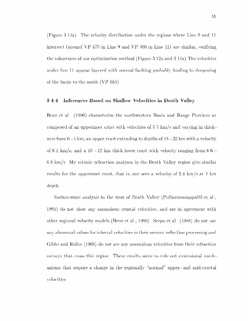
55

(Figure 3.14a). The velocity distribution under the regions where Line 9 and 11

intersect (around VP 475 in Line 9 and VP 300 in Line 11) are similar, verifying

the robustness of our optimization method (Figure 3.12a and 3.14a) The velocities

under line 11 appear layered with normal faulting probably leading to deepening

of the basin to the north (VP 664).

3.4.4 Inferences Based on Shallow Velocities in Death Valley

Benz et al. (1990) characterize the northwestern Basin and Range Province as

composed of an uppermost crust with velocities of 5.7 km/s and varying in thick-

ness from 0 - 4 km, an upper crust extending to depths of 18 - 22 kmwith a velocity

of 6.1 km/s, and a 10 - 12 km thick lower crust with velocity ranging from 6.6 -

6.8 km/s. My seismic refraction analyses in the Death Valley region give similar

results for the uppermost crust, that is, one sees a velocity of 5.8 km/s at 4 km

depth.

Surface-wave analysis to the west of Death Valley (Pullammanappallil et al.,

1994) do not show any anomalous crustal velocities, and are in agreement with

other regional velocity models (Benz et al., 1990). Serpa et al. (1988) do not use

any abnormal values for interval velocities in their seismic re ection processing and

Gibbs and Roller (1966) do not see any anomalous velocities from their refraction

surveys that cross this region. These results seem to rule out extensional mech-

anisms that require a change in the regionally \normal" upper- and mid-crustal

velocities.

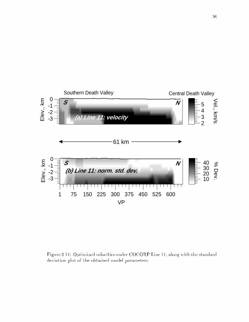
56

61 km

-3-2-10

Ele

v., km

2345

Ve

l., km/s

Central Death ValleySouthern Death Valley

(a) Line 11: velocity

S N

1 75 150 225 300 375 450 525 600VP

-3-2-10

Ele

v., km

10 20 30 40 %

De

v.

(b) Line 11: norm. std. dev.S N

Figure 3.14: Optimized velocities under COCORP Line 11, along with the standarddeviation plot of the obtained model parameters.

57

From the pure-shear point of view, these results require that extension within

the upper crust occurs by normal faulting. If this were the only extensional mech-

anism operating in the region, the amount of extension should be much less than

100%. It would require additional processes to operate in the lower crust (below

15 km) if the extreme extension observed by some workers (Wernicke et al., 1988)

is to be achieved. But the absence of Moho de ection or topographic depression in

areas where the crust has been denuded (Wernicke, 1985; Gans, 1987), compared

to the adjacent areas not denuded, seem to preclude any signi�cant interactions

between the upper mantle and lower crust and thus extension by a conventional

pure-shear mechanism.

This velocity analysis also constrains the conditions under which a simple-shear

based extension might operate in this region. If this occurs by the \ uid-layer"

hypothesis (Wernicke, 1992; Jones et al., 1992), the normal velocities we observe

would require the compensating medium to be very close in density to the upper

crust. This would imply that this \layer" is rich in quartz. Thus, to conclude,

the results favor the simple-shear mechanism over the pure-shear method as the

possible mechanism for extreme extension in the Death Valley region.

3.5 Imaging the o�shore Hosgri Fault, California

Pre-stack migrations that employ curved rays (Louie et al., 1988; Louie and Qin,

1991) are widely used to image structures in regions where velocity undergoes

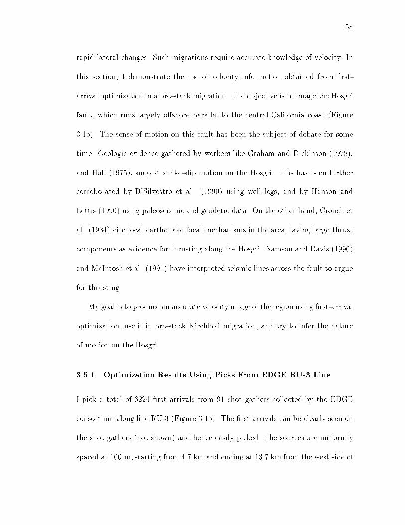
58

rapid lateral changes. Such migrations require accurate knowledge of velocity. In

this section, I demonstrate the use of velocity information obtained from �rst-

arrival optimization in a pre-stack migration. The objective is to image the Hosgri

fault, which runs largely o�shore parallel to the central California coast (Figure

3.15). The sense of motion on this fault has been the subject of debate for some

time. Geologic evidence gathered by workers like Graham and Dickinson (1978),

and Hall (1975), suggest strike-slip motion on the Hosgri. This has been further

corroborated by DiSilvestro et al. (1990) using well logs, and by Hanson and

Lettis (1990) using paleoseismic and geodetic data. On the other hand, Crouch et

al. (1984) cite local earthquake focal mechanisms in the area having large thrust

components as evidence for thrusting along the Hosgri. Namson and Davis (1990)

and McIntosh et al. (1991) have interpreted seismic lines across the fault to argue

for thrusting.

My goal is to produce an accurate velocity image of the region using �rst-arrival

optimization, use it in pre-stack Kirchho� migration, and try to infer the nature

of motion on the Hosgri.

3.5.1 Optimization Results Using Picks From EDGE RU-3 Line

I pick a total of 6224 �rst arrivals from 91 shot gathers collected by the EDGE

consortium along line RU-3 (Figure 3.15). The �rst arrivals can be clearly seen on

the shot gathers (not shown) and hence easily picked. The sources are uniformly

spaced at 100 m, starting from 4.7 km and ending at 13.7 km from the west side of

59

San Andreas fault

Rinconada-Nacimiento fault

San Simeon-San G

regorio fault

RU-13

PG&E-1

RU-3

PG&E-3

RU-5RU-2

RU

-10Hosgri fault

San Francisco

38.00 N

36.00 N

34.00 N

122 W

120 WN

Pacific Ocean

California

Figure 3.15: Generalized map showing the Hosgri fault, and some of the seismicpro�les traversing the area executed by Paci�c Gas and Electric (PG & E) andEDGE/Rice University (RU). Only shot gathers recorded along 13.7 km of theEDGE RU-3 line, crossing the fault and indicated by the thick line, are used inthis study.

60

the line. The average receiver spacing is about 75 m along the pro�le. The model

I use in the optimizations has dimensions of 15 km by 2.5 km with a grid spacing

of 50 m. The initial model has a constant velocity of 2 km/s and the velocity is

allowed to vary between 1.5 and 8 km/s during the annealing procedure. One of

the �nal models obtained after this is shown in Figure 3.16. The least-square error

reduces from 0.077 s2 to 0.00038 s2. Figure 3.16a shows the water layer (velocity

of 1.5 km/s) deepening away from the shore. About 2 km from the shore, one can

see a sharp change in velocity from 4 km/s to about 2.0 km/s. This transition

represents the Hosgri fault zone - rocks of the Fransiscan assemblage to the east

juxtaposed against marine sediments.

Figure 3.16 shows that the velocities are poorly constrained below 1.5 km. This

is manifested as higher normalized deviations (40 - 50 % ) in the statistical analysis

of models with comparable least-square error (Figure 3.16c). The maximumsource-

receiver o�set for this survey is only 4.5 km, which is probably why the rays do

not penetrate deeper than 1.5 km. The deviations are less than 0.3 km/s above

this depth.

The next step is to perform the pre-stack Kirchho� migration through the

velocity model obtained by annealing. Since the velocities beneath 1.5 km are

unconstrained, for the migration, I smooth the velocities to a depth of 2.5 km,

by linear extrapolation, and come up with the model shown in Figure 3.16d. The

pre-stack migration (method of Louie and Qin, 1991) takes into account curved

rays and has the ability to image near-vertical structures. Figure 3.17 shows the

61

-2.5-2.0-1.5-1.0-0.5

0

elev

, km

1.5 2.0 2.5 3.0 3.5 4.0 vel, km

/s

-2.5-2.0-1.5-1.0-0.5

0

elev

, km

1.5 2.0 2.5 3.0 3.5 4.0 vel, km

/s

-2.5-2.0-1.5-1.0-0.5

0

elev

, km

20

40

60 % dev

-15 -10 -5 0distance offshore, km

-2.5-2.0-1.5-1.0-0.5

0

elev

, km

1.5 2.0 2.5 3.0 3.5 4.0 vel, km

/s

sources & receivers

(a) anneal

(b) average

(c) norm. std. dev.

(d) smooth vel.

hosgri fault zone

EastWest

Figure 3.16: (a) Hosgri model obtained after the nonlinear optimization. Notethe sharp lateral change in velocity in the region delineated by the circle. Thearrow points at the Hosgri fault-plane image. (b) average model. (c) Standarddeviations normalized with respect to the average model (b). (d) The smoothedvelocity model used in the pre-stack migration to image the Hosgri fault.

62

pre-stack image. The high amplitudes delineated by the circle are the image of the

Hosgri fault. The artifacts associated with the migration obscure the sedimentary

sequence. But the sedimentary stratigraphy can be highlighted by performing a

post-stack migration (Figure 3.17, top panel). Imaging of sedimentary sequences

on both sides of the Hosgri allowed us to constrain vertical motions of the fault

to a maximum of 300 m in the past 5 million years (Honjas et al., 1992; Honjas,

1993).

3.6 Sub-surface Geometry of The Mojave Segment of the

San Andreas Fault

The most direct way of �nding the subsurface geometry of a fault would be to

correctly locate hypocenters in cross section. But, the Mojave segment of the San

Andreas fault (Figure 3.18) shows very little seismic activity compared to other

faults in the vicinity. Louie and Pullammanappallil (1994) show that a cross section

in this area does not show any apparent trend in the hypocenter locations (Figure

3.23). Thus one has to use other information, in conjunction with seismicity, to

delineate the fault at depth. Feng and McEvilly (1983) interpret fault locations

based on velocities got from seismic re ection and refraction surveys. This would

be e�ective only if fault zones are traceable as, say, low-velocity zone. Cheadle et

al. (1986) found that conventional common-midpoint stacking techniques break-

down in the presence of strong lateral velocity variations and are unable to focus

63

0

3

Dep

th, k

m

0 13.7Distance, km

-1.8e+04 1.8e+04Migrated Amplitude

Post-Stack

Pre-Stack

Post-Stack

Pre-Stack

0 13.7

3

Dep

th, k

m

Figure 3.17: Post- and pre-stack migration results. The post-stack migration usesa layered velocity model and images the horizontal sedimentary sequences well.Pre-stack migration through the model shown in Figure 3.16d can image near-vertical structures like the Hosgri fault. The circle delineates the high amplitudezone associated with the fault. The arrows indicate the Hosgri fault zone.

64

fault plane re ections. Hence, the most conclusive way to characterize the fault ge-

ometry will be an accurate velocity estimation followed by imaging the fault-plane

directly from multi-o�set seismic data.

First arrival times are picked o� shot gathers recorded along COCORP Mojave

line 1 (Figure 3.19). For the optimization the line is separated into two segments:

a northern segment from VP 61 to VP 271; and a southern segment that crosses

the San Andreas fault between VP 218 and VP 380 (Figure 3.18).

Further, to account for the bends in the line, the southern segment is projected

on to a line keeping the source-receiver o�set the same as the actual survey (Figure

3.18). The travel time picks are made from a total of 117 shot gathers.

3.6.1 Velocity Optimization: Results and Inferences

A total of 1518 �rst-arrival picks make up the data for the optimization of the

northern segment of the line. The average shot-spacing is about 200 m along this

segment. The constant velocity (5 km/s) starting model is 21.5 km long and 6 km

deep. The grid spacing is 125 m. Figure (3.20a) shows the velocity model, between

VP 61 and VP 271 and 21.1 km long, after the optimization. Only the upper 4 km

is shown since the parts of the model below it are poorly constrained. Uncertainties

associated with these velocities are determined as before. The model shows low-

velocity Tertiary basins north of Portal Ridge. The deviations in the velocities

become high (30%) only on the south side of the model below 2.5 km (Figure

3.20b). I compare the velocity result with those of Li et al. (1992) for this segment

65

0

10

12.44

San Andreas Fault

Mojave Desert

CO

CO

RP

Lin

e 1

VP 61

VP 218

VP 271

VP 380

Antelope Valley

Portal Ridge

34 51’15’’N, 118 19’15’’Wo o

o o34 37’30’’N, 118 24’44’’W

N

Transverse Ranges

Figure 3.18: Generalized map of the western-most Mojave desert showing theposition of the 1982 COCORP Mojave line 1, beginning at VP 61 and ending atVP 380. The section of the line used in the migrations (From VP 218) is shownby a thick line. The velocity optimization and the migrations were performed byprojecting the sources onto a line (shown with axis markings), while maintainingthe true source-receiver o�set. The axis labels are in kilometers.

66

0

4

Tim

e, s

-1.5

e+

03

1.5

e+

03

Co

rre

late

d A

mp

litu

de

SW NE

diffractions

281351 VP

Record #254Src VP 276

SAFZ

Record #256Src VP 280

285355 VP

SAFZ

NESWFigure 3.19: Raw shot gathers, from the south-west part of COCORP MojaveLine 1, showing di�ractions from the San Andreas fault zone. The location of thefault zone is also indicated. The �rst arrival picks from these gathers are used ina nonlinear optimization scheme to obtain velocities.

67

of line 1 (Figure 3.21). They obtain the result by ray tracing in conjunction with

conventional seismic processing. Both methods produces similar velocities within

the basins and of basement rocks. The depths to di�erent layers seem consistent.

The main di�erence is that the velocities I get by the nonlinear optimization fail to

delineate a over-thrust basin margin. The velocities reconstructed by the nonlinear

optimization also tend to be higher at depth.

588 picks along the southern segment were the input that produces the results

shown in Figure 3.20c. The model is 13 km and 6 km deep with a grid spacing of

125 m. The average shot-spacing along this projected segment is about 133 m.

Once again, only the better constrained upper 4 km and the region between VP

218 and VP 381 (12.44 km long) is shown in Figure 3.20c. The velocities do not

vary by more than 20% anywhere in the model (Figure 3.20d). Figure 3.20c shows

relatively low velocities within the fault zone (near VP 300, marked as SAFZ)

above 2 km depth, and relatively higher velocities just northeast of the surface

fault below 2 km. These velocities o�er the interpretation that if the San Andreas

fault zone is associated with lateral heterogeneity, then it dips 600 � 700 to the

northeast. There is no indication of any crustal low-velocity zone similar to the

one observed by Feng and McEvilly (1983) under the San Andreas fault in central

California. Thus, it is essential to perform a process that will directly image the

fault plane at depth.

68

61 100 150 200 271-4-3-2-10

dept

h, k

m

3456

vel, km/s

61 100 150 200 271-4-3-2-10

dept

h, k

m

102030 %

dev

(a) CM-1 North Segment Velocities

North South

(b) CM-1 North Segment Deviations

North South

218250300350381VP

-4-3-2-10

dept

h, k

m

23456

vel, km/s

-4-3-2-10

dept

h, k

m

0102030 % dev

12.44 km

(c) CM-1 South Segment Velocities

NortheastSouthwest

(d) CM-1 South Segment Deviations

218250300350381

SouthwestNortheast

VP

SAFZbasin

21.1 km

Figure 3.20: Velocities obtained from after the optimization. The top two panels(a and b) show the velocity and the percent deviations along the north-southsegment of the line. The bottom two panels (c and d) show the same for thesegment extending northeast to southwest.

69

21.1 kmVP

61

-4-3-2-10

de

pth

, km

3456

ve

l, km

/s

South North

Nonlinear Optimization

100300

-12

0

100150200271

2.6

7/5

.5

2.7

/5.5

2.75/62.67/5.5

2.23/3.25 2./3

2.81/6

from Li et al., 1992

Figure 3.21: Velocity model constructed by Li et. al (1992), for the north-segment of COCORP Line 1, is superimposed on the model got by using simulated-annealing. They use ray tracing and conventional seismic processing techniques.The numbers \2.75/6.0" correspond to density/velocity values and have unitsgm/cc and km/s respectively.

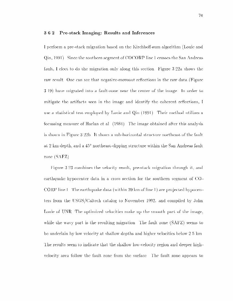
70

3.6.2 Pre-stack Imaging: Results and Inferences

I perform a pre-stack migration based on the Kirchho�-sum algorithm (Louie and

Qin, 1991). Since the southern segment of COCORP line 1 crosses the San Andreas

fault, I elect to do the migration only along this section. Figure 3.22a shows the

raw result. One can see that negative-moveout re ections in the raw data (Figure

3.19) have migrated into a fault-zone near the center of the image. In order to

mitigate the artifacts seen in the image and identify the coherent re ections, I

use a statistical test employed by Louie and Qin (1991). Their method utilizes a

focussing measure of Harlan et al. (1984). The image obtained after this analysis

is shown in Figure 3.22b. It shows a sub-horizontal structure northeast of the fault

at 2 km depth, and a 45o northeast-dipping structure within the San Andreas fault

zone (SAFZ).

Figure 3.23 combines the velocity result, pre-stack migration through it, and

earthquake hypocenter data in a cross section for the southern segment of CO-

CORP line 1. The earthquake data (within 20 km of line 1) are projected hypocen-

ters from the USGS/Caltech catalog to November 1992, and compiled by John

Louie of UNR. The optimized velocities make up the smooth part of the image,

while the wavy part is the resulting migration. The fault zone (SAFZ) seems to

be underlain by low velocity at shallow depths and higher velocities below 2.5 km.

The results seem to indicate that the shallow low-velocity region and deeper high-

velocity area follow the fault zone from the surface. The fault zone appears to

71

0

4

De

pth

, km

0 13Distance NE, km

-34.8 34.8Reflectivity

SW NE

CM-1 Pre-stack Migration, South Segment A

SAFZ

0

4

De

pth

, km

0 13Distance NE, km

-4 4Coherent Reflectivity

SW NESAFZ

CM-1 Focused Migration, South Segment B

Figure 3.22: (A) Pre-stack migration of muted �eld records (Figure 3.19) throughthe velocities obtained after the optimization (Figure 3.20c). (B) To emphasisedcoherent structures in the migrated section, a statistical method prescribed byHarlan et al. (1984) is used. The output mitigates some of the artifacts. The solidarrows in both panels indicate the trace of the dipping fault, as inferred from themigrations.

72

terminate at the sub-horizontal structure at a depth of 2.5 km. It is possible that

it represents the base of the Pelona Schist exposed at Portal Ridge, northeast of

the fault zone. The 450-dipping structure is probably the interface between schist

in the fault zone and the pre-Cambrian rocks in the Transverse Ranges. Based on

these results Louie and Pullammanappallil (1994) have hypothesized that the San

Andreas fault may be dipping northeast at 600 � 700 and that the seismicity in

this section is con�ned to the Transverse Ranges block.

3.7 Conclusions

I have demonstrated the use of a nonlinear optimization scheme based on simu-

lated annealing to obtain near-surface velocity information from �rst-arrival times.

The synthetic tests reveal that unlike a linearized-inversion scheme, the nonlinear

optimization does not depend on the initial model. This becomes important in

regions where we do not have any prior knowledge about subsurface velocity dis-

tribution. For the model sizes I use, the computation time for both methods was

comparable. The linearized inversions converge in fewer iterations, but expend

large computation times in matrix manipulations.

Annealing provides us with a suite of �nal models having comparable least-

square error. This allows us to choose a sub-set that best represents the geology

of the region. The optimization scheme samples a large region of the model space.

This property is put to use to compute the uncertainties associated with the �nal

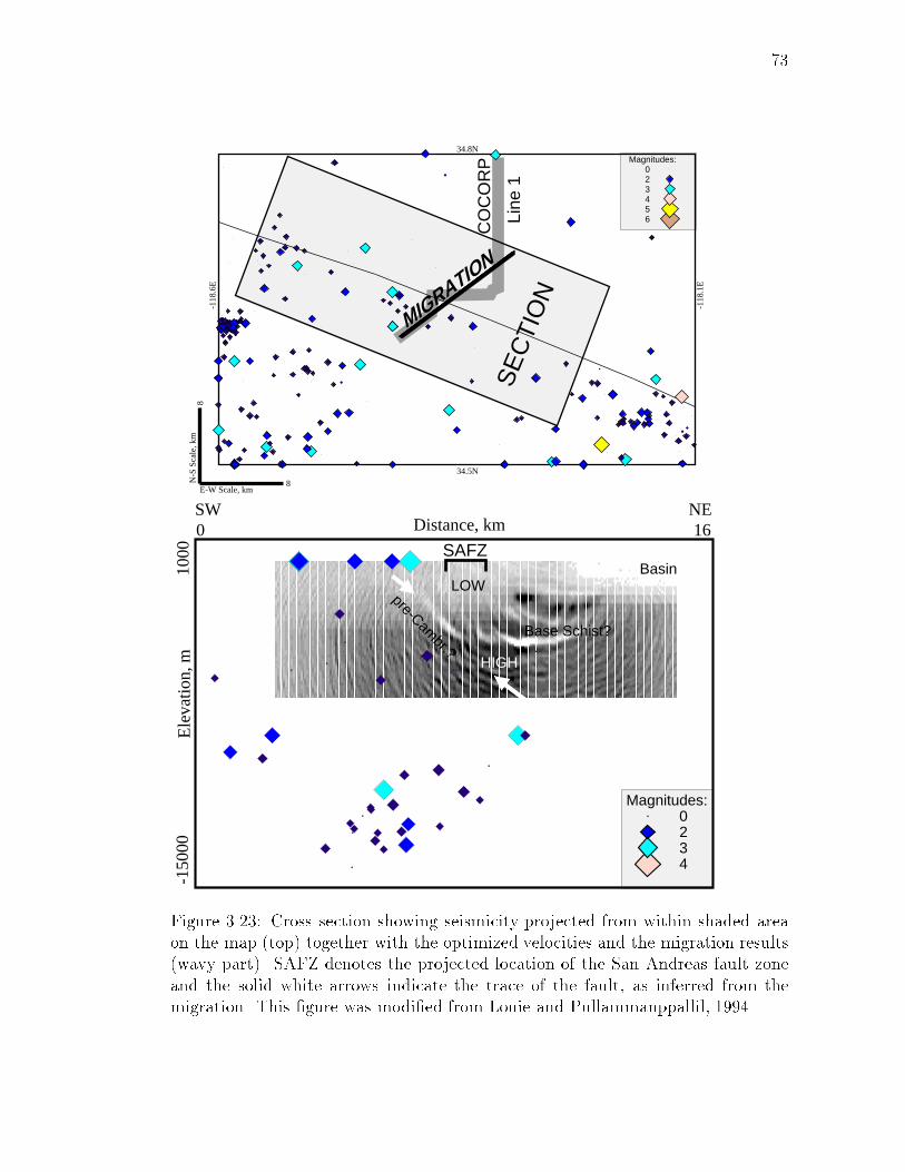
73

SE

CTI

ON

34.5N

34.8N

-118

.6E

-118

.1E

E-W Scale, km

N-S

Sca

le, k

m

8

8

654320

Magnitudes:

Ele

vatio

n, m

Distance, km0 16NESW

1000

-150

00

MIGRATION

Line

1

CO

CO

RP

4320

Magnitudes:

BasinSAFZ

LOW

HIGH

pre-Cambr.?

Base Schist?

Figure 3.23: Cross section showing seismicity projected from within shaded areaon the map (top) together with the optimized velocities and the migration results(wavy part). SAFZ denotes the projected location of the San Andreas fault zoneand the solid white arrows indicate the trace of the fault, as inferred from themigration. This �gure was modi�ed from Louie and Pullammanppallil, 1994.

74

model velocities. Through synthetic examples, I show that the normalized devia-

tions obtained do indeed correspond to the normalized absolute di�erence between

a \true" model and the optimization result. In addition tracing rays through the

results help to separate regions that are well constrained from regions that are not.

The �rst-arrival optimization has several applications. Two such uses are pre-

sented here. Obtaining shallow-crustal velocities can be important for understand-

ing the tectonic behavior of a region. Using data collected by COCORP, I image

the shallow-crustal velocities in the extended domain of the Death Valley region

of California. Near-surface velocities are also important for accounting for resid-

ual statics in re ection data processing. To show the robustness of the models

obtained by annealing, I compute vertical travel times through them. Finally, I

use the velocity model obtained from �rst-arrival picks to carry out a pre-stack

Kirchho� migration. This is done to image in cross-section the Hosgri fault and

the Mojave segment of the San Andreas fault, which lie in regions where the veloc-

ity changes laterally. The successful imaging of the faults demonstrates the ability

of the generalized simulated annealing to produce accurate velocity images of the

subsurface from �rst-arrival picks.

75

Chapter 4

Estimation of Velocities and Re ector Characteristics

From Re ection Travel Times Using a Nonlinear

Optimization Method

4.1 Abstract

In this chapter, the generalized simulated-annealing algorithm is extended to in-

vert seismic re ection times for velocities, re ector depths, and lengths. A �nite-

di�erence solution of the eikonal equation computes re ection travel times through

the velocity model and avoids ray tracing. I test the optimization scheme on syn-

thetic models and compare it with results from a linearized inversion. The syn-

thetic tests illustrate that, unlike linear inversion schemes, the results obtained

by the optimization scheme are independent of the initial model. The annealing

method has the ability to produce a suite of models which satisfy the data equally

well. This property is put to use to determine the uncertainties associated with

the obtained model parameters. Synthetic examples demonstrate that allowing

the re ector length to vary, along with its position, helps the optimization process

76

obtain a better solution. To test the performance of this method on real data,

I use it to image the Garlock fault, whose geometry at depth is poorly known.

I use re ection times picked from shot gathers recorded along COCORP Mojave

Line 5 to invert for the Garlock fault and velocities within the Cantil Basin be-

low Fremont Valley, California. The velocities within the basin obtained by the

optimization scheme are consistent with earlier studies, though the results suggest

that the basin might extend 1 - 2 km further south. The reconstructed re ector

seem to suggest shallowing of the dip of the Garlock fault at depth. I also show

including more information contained in the data, like �rst-arrivals, signi�cantly

improves the results.

4.2 Introduction

Determination of subsurface velocities is a di�cult proposition in areas where

lithology and structure undergo signi�cant lateral changes. Further complications

arise in re ection problems where the velocity as well as the re ector depth is not

known. The last decade has seen the development of numerous inversion schemes to

obtain velocity and re ector depth from re ection travel times. They have evolved

from the use of straight rays and �xed re ector depths (Kjartansson, 1980) to

more complicated ray tracing and simultaneous velocity-depth determination. We

can achieve simultaneous inversion in two ways. The �rst is to parameterize both

velocity and re ector depth and perform a joint inversion (e.g., Bishop et al., 1985;

77

Stork and Clayton, 1986a, b; Farra and Madariaga; 1988, Williamson, 1990). The

second approach is to use a migration technique to image the re ector with the

existing velocity �eld, then update the velocity keeping the re ector �xed (Bording

et al., 1987; Stork and Clayton, 1987). The main advantage of the second technique

is that it incorporates multiple arrivals from a re ector, while the joint inversions

use only �rst arrival re ections. However, the second technique is computationally

more expensive.

The objective of joint inversion is to minimize the least-square di�erence be-

tween the observed and calculated times through a model. This is cast as a gen-

eralized nonlinear least-squares problem (Tarantola and Valette, 1982; Tarantola,

1987). Farra and Madariaga (1988) solve this problem iteratively using the Gauss-

Newton method while Williamson (1990) uses an iterative subspace search method

to do the same. van Trier (1990a, b) simultaneously inverts for the re ector ge-

ometry and interval velocities using a Gauss-Newton method. Re ection times

depend on both the velocity and the depth of the re ectors, making travel time

inversion a nonlinear process. All the above methods involve local linearization

of the problem, and require the starting model to be close to the desired �nal

solution. I demonstrate this requirement later using synthetic models.

In this chapter, I examine the use of a nonlinear optimization scheme, namely

simulated annealing, to invert re ection travel times. I rapidly compute travel

times through models by a method avoiding ray tracing. It employs a fast �nite-

di�erence scheme based on a solution to the eikonal equation (Vidale, 1988). This

78

accounts for curved rays and all types of primary arrivals, i.e., the fastest arrival,

be it a direct arrival or a di�raction. I test the optimization process on synthetic

models and compare its performance with linear inversion schemes that use curved

rays. Synthetic examples and optimizations of data demonstrate that the method

is not dependent on the choice of the initial model. Another advantage of the

simulated-annealing algorithm is that it produces a suite of �nal models with

comparable least-square error. This enables one to choose the model most likely

to represent the geology of the region. This property is put to use to determine

the uncertainties associated with the model parameters obtained.

Lastly, I use the scheme to invert re ection times to image the Garlock fault

and the velocity within the Cantil Basin below Fremont Valley, California. The

travel time picks are made from the shot records of COCORP Mojave Line 5.

Strong lateral velocity variations across the basin make it di�cult to image the

Garlock fault by standard seismic velocity analysis techniques. The use of pre-

stack Kirchho� migration (Louie and Qin, 1991), which accounts for curved rays

and lateral velocity variations, requires prior knowledge of the velocities. This

makes it important to use an inversion scheme that will image the velocities with

minimum a priori constraints. In addition, the geometry of the Garlock fault

at depth is not unequivocally known. The nonlinear optimization scheme can

reconstruct velocities, as well as recover estimates of dip or length of the fault.

One need not specify the length or dip prior to the inversion.

79

4.3 Re ection Travel Time Calculation

Any inversion scheme requires the solution of the forward problem. In the present

case, the computation of re ection times through a known velocity �eld given

the re ector location constitutes the forward problem. I do this by a method

avoiding ray tracing. First, assume each point along the discretized re ector to be

a source and compute the travel times from these points using a �nite-di�erence

method (Vidale, 1988). The next step is to determine the re ection depth point

location for each source-receiver pair. For each source-receiver pair, I calculate

the total travel time by adding appropriate times, corresponding to all re ector

points (each one acting as a source). Invoking Fermat's principle, the minimum

total travel time will correspond to the time of primary re ection arrival. Thus

one can rapidly compute re ection times through any model given the velocity

and re ector location. Figure 4.1 shows a schematic representation of this process.

It also shows ray tracing through a test model using the above method, though

during the optimization I do not have to �nd any ray paths.

4.4 Results

In this section presents the results of the tests of the annealing optimization scheme

on synthetic models. In addition we also compare its performance with linear

inversion schemes that employ curved rays.

I use two synthetic models in the study, namely the three box model (Figure

80

reflector

possible ray paths

minimum time ray path

Shot

30

Shot

Receivers0

12

Receiver

(a)

(b)

dept

h, k

m

offset, km

diffraction

reflector

1.25 km/s1.0 km/s

Figure 4.1: (a) Schematic illustration of the use of Fermat's principle and seismicreciprocity to calculate re ection travel times. I use a �nite di�erence solution ofthe eikonal equation (Vidale, 1988) to calculate the direct arrivals (each ray). (b)Rays traced through a test model using the above method.

81

4.2a) and the lateral velocity gradient model (Figure 4.4a). The models are

30 km long and 8 km deep. There are sharp velocity contrasts in the three box

model, with slowness ranging from 0.75 s/km to 1.25 s/km. In contrast, the velocity

variation is gradual in the lateral gradient model (patterned after Williamson,

1990). Here the slowness varies between 0.382 s/km and 0.418 s/km. In both cases

the true re ector is fault-like, ranging between depths of 7 km and 5 km. There

are 30 sources each with 30 receivers along the top of the model, thus resulting in

900 travel time observations.

I �rst determine the critical temperature Tc. For the two synthetic cases Tc

was equal to 0.1. Accordingly I �x the cooling rate. Finally, before performing the

inversion, I determine the value of q. In this case q was equal to 2 for optimum

convergence. Figure 2.1 illustrates the above steps.

4.4.1 Optimization results of the three box model

The starting model has a slowness of 0.6 s/km and a at re ector at a depth of

6 km. I allow the slowness to vary between 0.6 s/km and 1.5 s/km while the

re ector can assume depths between 4 km and 7 km. Figures 4.2b and 4.2d show

the results of the optimization process. It reconstructs the high velocity region and

the background velocity well. But it fails to recover the low velocity boxes. This is

due to poor ray coverage in those regions. The rays bend around them and sample

the faster regions. As regards the re ector, the scheme recovers the sharp features

and the depth very well. The least-square error reduces from a value of 24.41 s2

82

0 10 20 30offset, km

-8

-6

-4

-2

0

dept

h, k

m 0.8

1.0

1.2

slowness, s/km

0 10 20 30offset, km

-8

-6

-4

-2

0

dept

h, k

m

0.8

1.0

1.2

slowness, s/km

0 10 20 30offset, km

-8

-6

-4

-2

0

dept

h, k

m

0.8

1.0

1.2

slowness, s/km

dept

h, k

m

offset, km

sources & receivers

trueinitial

annealsvd

(a)

(b)

(c)

(d)

Figure 4.2: Nonlinear optimization and linearized inversion results of the threebox model. (a) The true model, showing slowness and the re ector depth. Theinitial slowness for the optimization is 0.6 s/km. (b) The slowness model obtainedafter annealing. (c) Slowness model obtained from a linearized inversion schemeusing SVD. (d) The reconstructed re ector depth after annealing and a linearizedinversion. It also shows the true depth and initial depth.

83

number of iterations

number of iterations

leas

t sq.

erro

r (s

)le

ast s

q. e

rror (

s )

22

(a)

(b)

no accepted models

Figure 4.3: Least square error variation during the optimization of the three boxmodel. (a) The initial stages of the process (note the rapid variation in the leastsquare error). (b) The �nal stages. The gaps in the curve are regions of no acceptedmodels.

84

for the initial constant velocity and at re ector model to 0.0578 s2 for the �nal

model (Figure 4.3). From the �gure one can see that during the initial stages of the

optimization, when T is high, the least-square error varies rapidly. This indicates

that it tests numerous models and can easily escape from a local minimum. As

the optimization progresses, T becomes smaller, the probability of escaping local

minima also decreases. The optimization settles into the deepest minimum. This

shows that the choice of Tc and the cooling rate a�ect the convergence of the

annealing process.

4.4.2 Optimization results of the lateral gradient model

The initial model is one of constant slowness, with a value of 0.3 s/km, and has

a at re ector 6 km deep. During the inversion, the slowness can assume values

between 0.3 s/km and 0.5 s/km. Figures 4.4b and 4.4d show the annealing results.

The optimization scheme does a poor job of recovering the small lateral variations;

it reconstructs only the average velocity. On the other hand, it images the re ector

depth and shape very well. The recovered re ector is a smoothed version of the

true re ector, whereas the linearized scheme recovers a heavily averaged shape.

The least-square error decreases from 2.97 s2 for the initial model to 0.0085 s2 for

the �nal model.

85

0 10 20 30offset, km

-8

-6

-4

-2

0

dept

h, k

m 0.38 0.40 0.42 0.44 0.46

slowness, s/km

0 10 20 30offset, km

-8

-6

-4

-2

0

dept

h, k

m

0.38 0.40 0.42 0.44 0.46

slowness, s/km

0 10 20 30offset, km

-8

-6

-4

-2

0

dept

h, k

m

0.38 0.40 0.42 0.44 0.46

slowness, s/km

dept

h, k

m

offset, km

sources & receivers

trueinitial

svdanneal

(a)

(b)

(c)

(d)

Figure 4.4: Nonlinear optimization and linearized inversion results of the lateralgradient model, patterned after Williamson (1990). (a) The true model, showingslowness and the re ector depth. The starting slowness for the optimization is 0.3s/km. (b) The slowness model obtained after annealing. (c) Slowness modelobtained from a linearized inversion scheme using SVD. (d) The reconstructedre ector depth after annealing and after linearized inversion. It also shows thetrue depth and the initial depth.

86

4.5 Comparison with a linearized inversion scheme

In this section, I compare the performance of annealing with a linearized inversion

scheme. In the linearized inversion, I linearize the nonlinear relationship between

travel time and slowness and the re ector depth. Generally, this linear scheme

is cast in a matrix form and the solution obtained using a standard least-squares

technique (Jackson, 1972; Wiggins, 1972). I use a singular value decomposition

method to do this. Instead of solving for the perturbations to the model param-

eters, it compute a new model during each iteration (Shaw and Orcutt, 1985). I

compute the travel times by the same method used during annealing.

Figures 4.2 and 4.4 compare the results of the linearized inversion with those

from the nonlinear optimization scheme. Neither method recovers the velocity

well when there is a gradual lateral variation in the true model (Figure 4.4). The

range of the re ection travel times through the lateral gradient model is only

about 8 seconds while it is 23 seconds through the three box model. Hence,

the survey aperture might be too small to recover the slowness variations in the

former case. Annealing does better in recovering the sharp features of the model -

both in the case of velocity and of re ector shape. The smoothing applied during

the linearized inversion scheme helps convergence, but smears the velocities and

averages out the re ector depth. Both methods reconstruct the re ector depth

and shape fairly well close to the edges of the model. It is noteworthy that the

velocity above these regions are not well recovered. This can be attributed to

87

the inherent ambiguity in the simultaneous reconstruction of velocity and re ector

characteristics. It illustrates that velocity-depth trade-o�s near the re ector are

hard to resolve. In the tests the re ector depth is better resolved probably because

it is described by fewer parameters (30 as compared to 240 velocity parameters).

The second-di�erence smoothing applied during the linearized inversions and the

averaging during annealing also helps in reconstructing the re ector shape better.

The convergence of the linearized inversions is initial-model dependent (in the

synthetic tests the starting model is close the true solution for the linearized inver-

sions). To demonstrate this I do another synthetic test and use the slowness model

derived by Louie and Qin (1991) for their pre-stack migrations (which will be put

to further use later on) as the true model. The model has dimensions of 26 km by

7 km with a fault shaped re ector along the bottom as shown in the top panel of

Figure 4.5. The slowness varies between 0.2 s/km and 0.45 s/km. I assume the re-

ector position and shape are known, and invert for only the velocities. Twenty-six

receivers along the surface record travel times from twenty-six sources. Figure 4.5

shows inversion results of the linearized scheme using two di�erent starting mod-

els. The solutions are di�erent, though the least-square errors are comparable in

both cases. The inversion with an initial model of 0.2 s/km reconstructs the model

better (a global minimum) than the one with a starting slowness of 0.4 s/km (a

local minimum). Figure 4.6 shows the optimization results by annealing. The �nal

models obtained after starting with two di�erent models look similar. The random

perturbations used during the annealing scheme make it independent of the initial

88

model. It destroys any order in the starting model within the �rst few iterations.

The Laplacian smoothing applied during the inversion might explain the better

reconstruction of the low velocity (high slowness) basin in the linearized scheme.

Note that in both the methods, the region below the re ector is unconstrained

due to absence of any ray coverage. Thus, even when we eliminate the nonlinear-

ity due to simultaneous dependence of re ection travel times on the velocity �eld

and re ector depth, by keeping the re ector position �xed, the linearized inversion

scheme shows dependence on the initial model. Though the linearized inversion

takes fewer iterations to converge, more time is spent in the matrix operations,

making the total computation time, for the problem to converge, comparable in

both cases.

For the nonlinear optimization scheme, the computation time is proportional

to the size of the model and the number of re ector nodes. Models with 1500 cells

and a re ector along the whole length took about 60 hours on a SPARCstation

2. With a grid spacing of 250 m and for a survey line 15 km long, this would

mean one can invert for velocities and re ector depths down to 7 km in the above

mentioned time.

4.6 Imaging the Garlock Fault, Cantil Basin

The left-lateral Garlock fault branches into two strands in the Fremont Valley,

California, region. The eastern branch strikes almost east-west while the western

89

branch strikes southwest-northeast (Figure 4.7). Cantil Basin itself is a pull-apart

basin, and Aydin and Nur (1982) show that it is one of the largest of its kind in

the San Andreas fault system.

The Consortium for Continental Re ection Pro�ling (COCORP) Mojave Line 5

collected seismic re ection data across the Garlock fault in Fremont Valley (Figure

4.7). Stacked sections of Line 5 displayed by Cheadle et al. (1986) show portions of

the basin oor and the southern wall. However, strong lateral velocity variations

across the basin made the imaging inadequate. Louie and Qin (1991) used a

pre-stack Kirchho� migration, which accounts for curved rays and lateral velocity

variations, on the Line 5 data. They infer that Cantil Basin was either a negative

ower structure, or a detachment headwall with the Garlock fault attening at

depth. They prefer the detachment model since it allows a simple mechanism to

explain the observed broadening of Cantil basin with fault movement over time.

Kirchho� migration assumes prior knowledge about the velocity. Hence, an

iterative application of this method would demand the initial model be close to the

solution to keep it computationally inexpensive. Use of the nonlinear optimization

will not require any constraints on the model. Since one of the goals is to determine

the nature of the fault at depth, one does not put any constraints either on the

location or the shape of the fault (the re ector). Resolving the structure of the

Garlock fault and Cantil Basin would help constrain regional tectonics, mainly the

con�guration of the Mojave block.

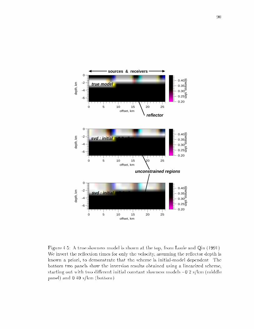
90

0 5 10 15 20 25offset, km

-6

-4

-2

0de

pth,

km

0.20

0.25

0.30

0.35

0.40

slowness, s/km

0 5 10 15 20 25offset, km

-6

-4

-2

0

dept

h, k

m

0.20

0.25

0.30

0.35

0.40

slowness, s/km

0 5 10 15 20 25offset, km

-6

-4

-2

0

dept

h, k

m

0.20

0.25

0.30

0.35

0.40

slowness, s/km

sources & receivers

true model

svd : initial = 0.2 s/km

svd : initial = 0.4 s/km

unconstrained regions

reflector

Figure 4.5: A true slowness model is shown at the top, from Louie and Qin (1991).We invert the re ection times for only the velocity, assuming the re ector depth isknown a priori, to demonstrate that the scheme is initial-model dependent. Thebottom two panels show the inversion results obtained using a linearized scheme,starting out with two di�erent initial constant slowness models - 0.2 s/km (middlepanel) and 0.40 s/km (bottom).

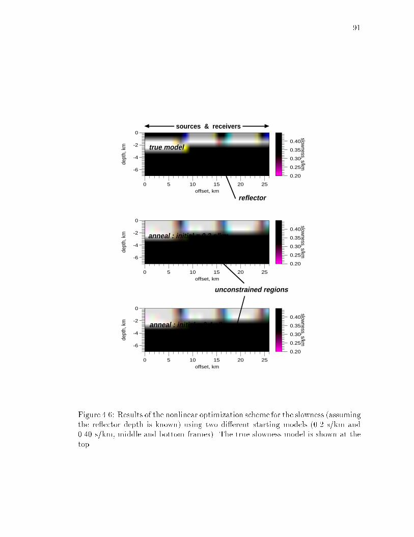
91

0 5 10 15 20 25offset, km

-6

-4

-2

0

dept

h, k

m

0.20

0.25

0.30

0.35

0.40

slowness, s/km

0 5 10 15 20 25offset, km

-6

-4

-2

0

dept

h, k

m

0.20

0.25

0.30

0.35

0.40

slowness, s/km

0 5 10 15 20 25offset, km

-6

-4

-2

0

dept

h, k

m

0.20

0.25

0.30

0.35

0.40

slowness, s/km

sources & receivers

true model

anneal : initial = 0.2 s/km

anneal : initial = 0.4 s/km

unconstrained regions

reflector

Figure 4.6: Results of the nonlinear optimization scheme for the slowness (assumingthe re ector depth is known) using two di�erent starting models (0.2 s/km and0.40 s/km, middle and bottom frames). The true slowness model is shown at thetop.

92

4.6.1 Results of the travel time inversion

The data I use are re ection times picked from shot gathers (Figure 4.8). These

shot gathers are recorded along Line 5 between VP (vibrator point) 240 and VP

382 (Figure 7). Louie and Qin (1991) compute synthetic seismograms to show that

these are re ections o� the east branch of the Garlock fault. The total number

of observations is 621 re ection times (a picking error of 0.02 s), picked from

28 shot gathers. The pacing between the shots is 100.5 m along the line. In

order to determine an optimum grid spacing to use in the inversions, I perform

a convergence test (not shown). I compute travel times through models with the

same dimensions, but di�erent grid spacings. For a range of grid spacings the

optimum spacing is that for which smaller spacings did not appreciably alter the

computed times (i.e.: less than the error in the data). The dimensions of the model

were 14.4 km by 4 km with a grid spacing of 277.85 m. I incorporate elevation

corrections by extrapolating the times to sources and receivers not on the grid,

assuming plane-wave propagation between grid points.

Before embarking on the optimization process, it is essential to determine

whether letting the re ector length vary hinders the inversion from reaching the

solution. For this study the true velocity model is the one used by Louie and Qin

(1991) for the Cantil Valley region. The source-receiver con�guration is same as

the actual survey. The shape of the re ector corresponds to the dip of the east

branch of the Garlock fault shallowing at depth. It has a dip of about 50 degrees

93

near the surface, changing to about 30 degrees at 2.5 km depth (Figure 4.9a). I

do two optimization runs - one keeping the re ector length �xed and equal to the

true length, and the other letting the length vary.

From Figure 4.9b we see that keeping the re ector length �xed hinders the

optimization process. The velocity and re ector are reconstructed poorly. This is

an example of a bad choice of the objective function. The annealing process does

a better job of reconstructing the velocities and re ector shape when the re ector

length is allowed to vary (Figure 4.9c), suggesting that it is a more useful objective

function. The optimization reconstructs only the lower part of the re ector because

the picked re ections see only this segment of the true re ector. This is shown in

a later section.

Hence during the data optimizations, I let the re ector length vary along with

its position. The length can be as short as 277.85 m (the grid spacing) or as long

as 14.4km (the length of the model). The re ector position can vary from near

surface to 4 km depth. Hence, the re ector can assume any dip and the dip can

change along its length. Each cell in the model can assume any velocity between

1.5 km/s and 6.3 km/s, the range of velocities expected in this region. I perform

the optimization with three di�erent constant velocity starting models - 2.5 km/s,

4.0 km/s and 8.3 km/s. We see that (Figure 4.10) the �nal model in all three cases

are similar, even if we start out with the unreasonably high velocity of 8.3 km/s.

The features that are common to all three results would be the most reliable.

The inversion reconstructs a prominent low velocity basin (2.4 - 2.6 km/s)

94

Southw

est B

ranch

East Branch Garlock Fault

Garloc

k Fau

lt

Lin

e 5

VP 240

VP 382 Cantil Valley

Sie

rra N

evada.

Blackwater Flt.

Harper Flt

Lockhart Flt.

South Lockhart Flt.

Se

irra

Ne

va

da

Flt.

N

0 15km

35.7 N

35.0 N

-1

18

.5 W

-1

17

.0 W

Figure 4.7: Generalized map showing the location of COCORP Line 5 crossingthe Garlock fault in Southern California. This study uses shot gathers recordedbetween VP 240 and VP 382. Some nearby faults are also identi�ed.

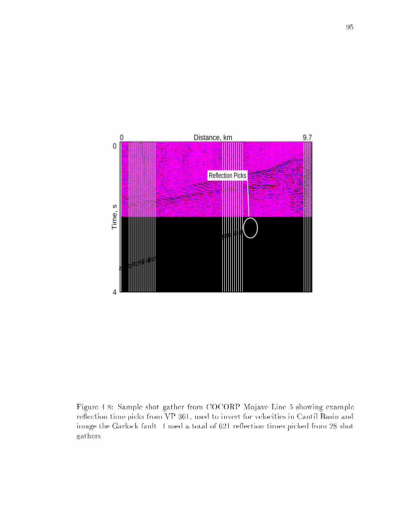
95

Tim

e, s

Distance, km

Reflection Picks from VP 3610 9.7

0

4

233233233233233233233233233233233233233233233233233233233233233233233233233233

233233233233233233233

Reflection Picks

Figure 4.8: Sample shot gather from COCORP Mojave Line 5 showing examplere ection time picks from VP 361, used to invert for velocities in Cantil Basin andimage the Garlock fault. I used a total of 621 re ection times picked from 28 shotgathers.

96

240 260 280 300 320 340 360 380Receiver VP

-4

-3

-2

-1

0de

pth,

km

2.5

3.0

3.5

4.0

4.5

5.0

velocity, km/s

240 260 280 300 320 340 360 380Receiver VP

-4

-3

-2

-1

0

dept

h, k

m

3.0

3.5

4.0

4.5

5.0 velocity, km/s

240 260 280 300 320 340 360 380Receiver VP

-4

-3

-2

-1

0

dept

h, k

m

3.5

4.0

4.5

5.0 velocity, km/s

14.4 km

recovered reflector

true reflector

true model

fixed refl. length

var. refl. length

South North

South North

sources(a)

(b)

(c)

Figure 4.9: Results of the synthetic study using a velocity model for the regionfrom Louie and Qin (1991) and keeping the source-receiver con�guration the sameas the actual survey. (a) The true model, with the part of the re ector seen bypicked re ection rays delineated by the square. (b) Optimization result when there ector length is kept �xed and equal to the true length. (c) The reconstructedvelocity and re ector (broken line) when the re ector length is allowed to varyduring the optimizations. The true re ector (solid line) is shown for comparison.

97

whose location corresponds to that of Cantil Basin. The basin seems to extend

1 - 2 km further south than suggested by Louie and Qin (1991) and may be 2 to

2.5 km deep. The re ector is about a kilometer long and extends from a depth of

3 km to about 3.5 km. The dip of this segment of the re ector is between 20 to

30 degrees and it lies beneath the low velocity basin. If this is interpreted as part

of the Garlock fault, it indicates that the fault shallows at depth, since di�raction

studies (Louie and Qin, 1991) indicate that the fault dips about 45 degrees near

the surface. The least-square error decreases from 3.48 s2 for the constant velocity

starting model to 0.00445 s2 for the �nal model. The travel time residual between

the �nal model and the data is less than 0.1 seconds for all the observations. The

range of the observed travel times was between 2.25 and 3.65 seconds.

By using three di�erent initial models, I allow the optimization process to sam-

ple di�erent parts of the model space. It approaches the minimum least-square

error from di�erent directions. Hence, I can use the �nal models, with compa-

rable least-square error, from each of the three runs to estimate the uncertainty

associated with the obtained model parameters. In this analysis, I use about 15

models from each run and thus a total of about 40 models. Figure 4.11a shows

the re ector points sampled by the rays for these models along with the recovered

re ector of the �nal model. Most of the midpoints cluster around the recovered

re ector. The standard deviation of the velocities (Figure 4.11b) range from 0.46

km/s to 0.85 km/s. It is important to note that these may not represent the ac-

tual deviations in the model parameters because of the nonlinear nature of the

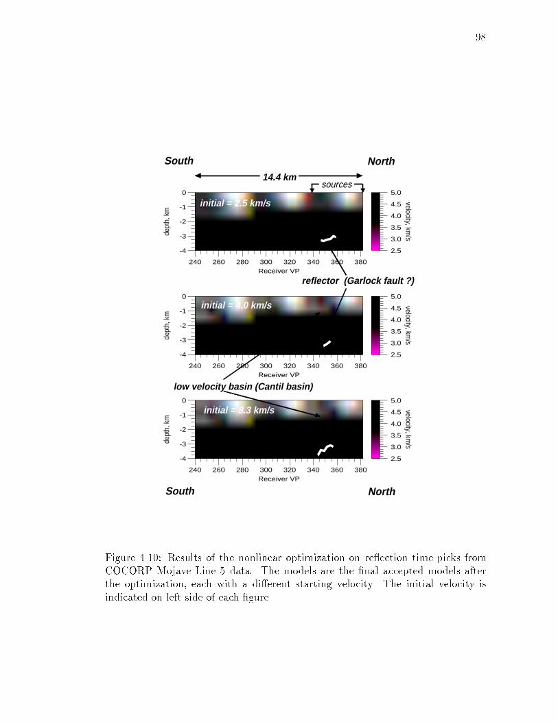
98

240 260 280 300 320 340 360 380Receiver VP

-4

-3

-2

-1

0

dept

h, k

m

2.5

3.0

3.5

4.0

4.5

5.0

velocity, km/s

240 260 280 300 320 340 360 380Receiver VP

-4

-3

-2

-1

0

dept

h, k

m

2.5

3.0

3.5

4.0

4.5

5.0

velocity, km/s

240 260 280 300 320 340 360 380Receiver VP

-4

-3

-2

-1

0

dept

h, k

m

2.5

3.0

3.5

4.0

4.5

5.0

velocity, km/s

14.4 km

initial = 2.5 km/s

initial = 4.0 km/s

initial = 8.3 km/s

South North

South North

sources

reflector (Garlock fault ?)

low velocity basin (Cantil basin)

Figure 4.10: Results of the nonlinear optimization on re ection time picks fromCOCORP Mojave Line 5 data. The models are the �nal accepted models afterthe optimization, each with a di�erent starting velocity. The initial velocity isindicated on left side of each �gure.

99

problem. It is di�cult to separate out the contributions due to mislocation of the

re ector and the errors in the velocities. But it does provide an idea about well-

and poorly-resolved regions in the model. The statistical analysis is performed

over accepted models only. So there might be unconstrained regions in the model

which are not perturbed, and hence have a small deviation. But, in general, the

regions with higher standard deviation are parts of the model that have poor ray

coverage. Hence, changing velocities in these regions do not a�ect the calculated

travel times much and thus contribute minimally to the least-square error.

The synthetic study using the velocity model constructed by Louie and Qin

(1991) for the region and the actual survey's source-receiver con�guration (Figure

4.9c), indicate that the scheme recovers velocities in and around the low velocity

basin to within 0.5 km/s to 1.0 km/s. The resolution decreases with distance from

and depth below the basin. This approximately corresponds to the deviations

obtained from the statistical analysis on the models obtained using the real data.

This study also shows that the optimization images only the lower part of the

re ector, suggesting that the small segment of the re ector imaged during the

data optimization is fairly robust.

The poor imaging of the re ector is probably related to the source-receiver

con�guration of the survey, that is, all the sources are towards the north side of

the model and most of the receivers to the south. To con�rm this, I determine the

depth points along the re ector for every source-receiver pair in a manner similar

to how we compute the travel times. I plot these along the true re ector in Figure

100

4

240 260 280 300 320 340 360 380Receiver VP

-4

-3

-2

-1

0

dept

h, k

m

0.5

0.6

0.7

0.8 velocity, km/s

0

dept

h, km

240 382Receiver, VP

14.4 km

recovered refl.

(a)

(b)

Figure 4.11: (a) Re ection depth points for the models used to determine thedeviations in the velocities. The recovered re ector for one of the �nal models isshown by the solid line. (b) Uncertainties associated with the velocities obtainedafter the nonlinear optimization scheme.

101

4.9a (delineated by a square). This shows that the picked re ection rays see only

the lower part of the re ector. Thus poor ray coverage causes the steeply-dipping

part not to be reconstructed and might also explain the poor reconstruction of

velocities away from the basin.

This study identi�es features of the model that are and are not robust. For

these optimizations I use only the primary re ected arrivals and a small subset of

the data (only 28 shot gathers along Line 5). In contrast, the pre-stack Kirchho�

migration (Louie and Qin, 1991) uses all types of arrivals and more data (228 shot

gathers), to image the Garlock fault. So including more data in the optimizations

could enable one to image more of the fault.

4.6.2 Including First-Arrival Travel Times

To see if I can better constrain the velocities and reconstruct more of the re ec-

tor, I include information from �rst-arrival times in the optimization. I picked

611 �rst-arrival times from the 28 shot gathers used for the re ection travel time

optimization. First-arrival times can be easily picked, and so I have more observa-

tions. Simulated-annealing optimizations, as described in Chapter 3, using these

times produce the velocity model shown in Figure 4.12 (top panel). I obtain well-

constrained velocities down to 1 km. Now, using this as an a priori constrain, I

repeat the optimization for the re ection travel times. The bottom panel of Figure

4.12 shows the results of using the optimization. Velocities can now be resolved

down to 5 km, compared to 3.9 km when only re ection picks are used. More of

102

the dipping part of the re ector is reconstructed and can be traced almost to the

surface. The at part of the re ector might be a \bottom of the model" e�ect. Us-

ing �rst-arrivals increases the resolution of velocities within the low-velocity basin.

The lowest velocity, now recovered, is 1.67 km/s within the Cantil basin (Figure

4.12-top) as opposed to 2.5 km/s before (Figure 4.10). Thus, by including more

information contained in the data, we can better resolve the model parameters.

4.7 Conclusions

In this chapter I presented a nonlinear optimization scheme to invert seismic re-

ection travel times, tested it on synthetic data and used it to image the Garlock

fault and velocities within Cantil Basin.

The synthetic study using the three box model and lateral gradient model

demonstrate the inherent ambiguity in recovering the velocity and re ector depth

from re ection travel times. But the nonlinear optimization scheme avoids local

linearization of the problem, allowing it to settle into a global (or deepest) min-

imum. The random perturbations that go into the optimization process make

it independent of the initial model. The method provides for easy implementa-

tion of constraints. It facilitates inversion for the re ector depth, its length and

shape. The method does not involve matrix inversion; hence it is computationally

tractable. The need to perform numerous iterations make the scheme computa-

tionally intensive when the depth of interest becomes greater than 10 km, for grid

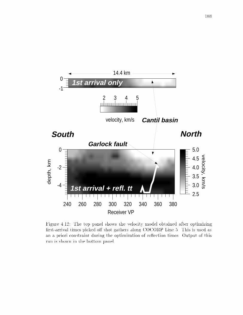
103

-1

0

2 3 4 5

velocity, km/s

240 260 280 300 320 340 360 380Receiver VP

-4

-2

0

de

pth

, km

2.5

3.0

3.5

4.0

4.5

5.0

ve

locity

, km

/s

14.4 km

1st arrival + refl. tt

1st arrival only

South North

Cantil basin

Garlock fault

Figure 4.12: The top panel shows the velocity model obtained after optimizing�rst-arrival times picked o� shot gathers along COCORP Line 5. This is used asan a priori constraint during the optimization of re ection times. Output of thisrun is shown in the bottom panel.

104

sizes used in the above studies.

The velocities obtained by this optimization scheme within Cantil basin (2.4 -

2.6 km/s) are consistent with earlier studies using gravity data, refraction data and

Kirchho� migration. The depth of the basin is about 2.5 km and seems to extend

further south than suggested by previous studies. The synthetic study shows that

the small segment of the re ector recovered by the optimization process is robust.

By including more information contained in the data, namely �rst-arrivals, the

depth of the resolved velocities increases to 5 km. Consequently more of the

re ector is reconstructed. This indicates that the dip of the Garlock fault shallows

at about 5 km. We are also able to trace it almost to the surface. This is consistent

with the detachment model suggested for the Mojave region by Louie and Qin

(1991). Thus, using only the primary re ected arrivals and �rst-arrivals from a

small data set I am able to obtain velocities within the basin and image a segment

of the fault.

Successful application of the nonlinear optimization scheme to image the Gar-

lock fault and Cantil basin suggests that the method is very useful in regions where

there are strong lateral velocity variations and where neither the fault shape nor

depth are known. I demonstrate that inverting for the re ector length is crucial

for the optimization to �nd the best solution. This feature makes the scheme more

attractive, since generally we do not know the extent of subsurface structures.

Though the recovered re ector is only a collection of depth points, it gives us an

idea of the location and nature of the re ector. This information, along with the

105

reconstructed velocity model, can be used in a pre-stack migration (which uses all

arrivals) to recover �ner details along the re ector.

106

Chapter 5

A Combined First-Arrival Travel Time and Re ection

Coherency Optimization Approach to Velocity Estimation

5.1 Abstract

The previous chapters presented the use of travel times, both re ection and �rst-

arrivals, to obtain velocity estimates. This chapter presents a method to include

amplitude information present in the data along with the travel times. To achieve

this, I design a simulated-annealing algorithm to simultaneously minimize �rst-

arrival travel time residuals and maximize re ection coherency. The shallow veloc-

ity structure is constrained by the �rst-arrival times, while coherency information

from deeper re ectors (if present) helps constrain the velocities at depth. A pre-

stack migration through the �nal velocity model images the re ectors directly.

Annealing, being a Monte-Carlo based algorithm, extensively samples the model

space. I exploit this property to identify the well-resolved areas of the velocity

model. Synthetic and real data examples demonstrate that migration through

velocities obtained using this method are more robust than those using only �rst-

arrival times. The data examples use shot gathers collected along COCORP Line

107

5 across the Garlock fault in Cantil Valley, California and COCORP Line 1 that

crosses the Mojave segment of the San Andreas fault. Imaging re ectors and esti-

mating velocities using annealing provides an alternative to picking re ection times

from shot gathers recorded over regions with complex geology.

5.2 Introduction

Travel time inversion su�ers from an inherent re ector depth-velocity ambiguity

(Stork, 1992a, b). One way to resolve this ambiguity is to make use of additional

information contained within the data. Including amplitude information is one

such method. Pre-stack migration achieves this purpose, but then it requires prior

knowledge of the velocity model. Conventional velocity analysis methods such as

semblance analysis (Toldi, 1989), focusing analysis (Yilmaz and Chambers, 1984),

and migration moveout analysis (Al-Yahya, 1989) are done interactively. This

could prove to be di�cult in areas underlain by complex structures. Another ap-

proach to velocity estimation is by travel-time inversion. The depth of resolution

is limited by the type of arrivals used � �rst arrivals constrain the near-surface

velocities, while re ections provide deeper information. Usually travel time in-

version with re ected arrivals is performed using times picked o� one re ecting

horizon. This leads to poor ray coverage in several areas of the model. Moreover,

it is often di�cult to pick re ection times from shot gathers. To overcome some

of these problems several workers have tried to combine the pre-stack migration

108

and re ection tomography. One such method casts the migration as a linearized

inversion problem (Ehinger and Lailly, 1993). But the need to solve a large linear

system makes this method computationally expensive. Jervis and Sto�a (1993)

use a genetic algorithm to estimate velocities. Instead of using a travel time min-

imization, their objective function was based on a di�erential semblance operator

(Symes and Carazzone, 1991). Their approach required iterative migration, and

to keep the computation time tractable they had to de�ne the velocities as spline

functions.

I base my approach on the formalism of Landa et al. (1989). They perform the

inversion in two steps. First, for a given velocity distribution, they map the depth

to re ectors using zero-o�set travel time information. Next, the velocity model

is updated using the re ection coherency criterion. Their method require the

velocity model be layered. The interface positions and velocity within each layer

need to be spline functions. The method developed here di�ers from the above in

that I use both travel time and amplitude information simultaneously, and and I

perform a pre-stack migration only once through the �nal velocity model. I do not

assume any prior velocity distribution in the models. First-arrival times (which

can be picked easily) provide us information about the shallow horizons, while

coherency computed from re ection times should constrain velocities in deeper

horizons. Performing a pre-stack migration through the velocity model obtained

after the optimization images many re ectors at the same time. Using simulated

annealing to do the optimization avoids linearizing the problem and the problem

109

of the inversion being trapped in a local minima.

I demonstrate the utility of this technique using synthetic and real data. For

the synthetic tests I use the velocity model derived by Louie and Qin (1991) for the

Cantil basin straddled by the Garlock fault in Cantil Valley (Figure 5.1c). I choose

this model because one of the real data set comes from this region. Hence, in ad-

dition to testing the e�ectiveness of the method, it will also serve as a resolution

study. The real data examples come from two sets of shot gathers: 1) northern seg-

ment of the COCORP line 5 crossing the Garlock fault in Cantil Valley, California;

and 2) southern segment of the COCORP line 1 that crosses the Mojave segment

of the San Andreas fault. I compare the velocity estimates and the corresponding

pre-stack images obtained by using the combined coherency��rst-arrival approach

and those obtained by using only �rst-arrival times. In addition, I also how this

method compares to using only re ection travel times.

5.3 Method

The objective function is made up of two parts:

1. The least square di�erence between the picked �rst-arrival times (tobs) and

those calculated through the velocity model (tcal). I denote this as Ett and

it is given by the expression,

Ett =1

n(

nXl=1

(tobsl � tcall )2) (1)

110

where n is the number of observations.

2. Re ection coherency as de�ned by Landa et al., 1989. This is given by the

equation:

Scoh =Xi

KXk=0

(P

j Uij [k�t+ � ])2Pj(Uij[k�t+ � ])2

(2)

where Uij represents the seismic trace for the ith source and jth receiver, �

is the calculated travel time, �t is the sample interval, and k�t is the time

window for the semblance calculation.

The objective of this optimization is to simultaneously minimize equation (1) and

maximize (2). I achieve this by employing a Monte-Carlo based technique called

simulated annealing. The advantages that stem from the nonlinear nature of this

optimization process have been documented by several workers (e.g., Sen and

Sto�a, 1991; Pullammanappallil and Louie, 1993). By using it in this problem

I demonstrate its ability to optimize multiple objective functions simultaneously.

This allows us to utilize more information from the data space, which could be of

di�erent scales, to get more robust solutions in the model space.

Implementation

I extend the single-objective function method developed in Pullammanappallil

and Louie (1993) to tackle the present problem. I start with a constant velocity

model and a at re ector along the bottom of the model. Each iteration involves

perturbing the velocity model and the re ector characteristics. I vary the length,

shape, and position of the re ector. I use a fast �nite-di�erence solution to the

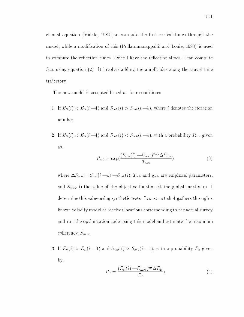
111

eikonal equation (Vidale, 1988) to compute the �rst arrival times through the

model, while a modi�cation of this (Pullammanappallil and Louie, 1993) is used

to compute the re ection times. Once I have the re ection times, I can compute

Scoh using equation (2). It involves adding the amplitudes along the travel time

trajectory.

The new model is accepted based on four conditions:

1. If Ett(i) < Ett(i� 1) and Scoh(i) > Scoh(i� 1), where i denotes the iteration

number.

2. If Ett(i) < Ett(i� 1) and Scoh(i) < Scoh(i� 1), with a probability Pcoh given

as,

Pcoh = exp((Scoh(i)� Smax)qcoh�Scoh

Tcoh) (3)

where �Scoh = Scoh(i� 1) � Scoh(i), Tcoh and qcoh are empirical parameters,

and Smax is the value of the objective function at the global maximum. I

determine this value using synthetic tests. I construct shot gathers through a

known velocity model at receiver locations corresponding to the actual survey

and run the optimization code using this model and estimate the maximum

coherency, Smax.

3. If Ett(i) > Ett(i� 1) and Scoh(i) > Scoh(i� 1), with a probability Ptt given

by,

Ptt =(Ett(i)� Emin)qtt�Ett

Ttt) (4)

112

where �Ett = Ett(i � 1) � Ett(i), Ttt and qtt are parameters determined

empirically, and Emin is the value of the objective function at the global

minimum, ideally equal to zero.

4. If Ett(i) > Ett(i� 1) and Scoh(i) < Scoh(i� 1), with a probability P, de�ned

as:

P = Pcoh � Ptt (5)

where the above indicates the probability of accepting models with less re-

ection coherency provided they are �rst accepted with a probability of Ptt.

I determine the parameters Tcoh, Ttt, qcoh, and qtt by a procedure described in detail

by Pullammanappallil and Louie (1993, 1994). It involves doing several short runs

of the algorithm for various �xed temperature values and computing the average

least square error for each run. This gives us the critical temperature Tc which in

turn determines how Ttt and Tcoh are varied during the optimization. A similar

procedure determines qtt and qcoh.

5.4 Results From Synthetic Test

This section presents the results of using this technique on synthetic data. The

true velocity model I choose (Figure 5.1c) is based on refraction velocity in the

area from which the real data comes from (Louie and Qin, 1991). Thus it has the

low-velocity sediments associated with the Cantil basin, which is bounded by the

branches of the Garlock fault. I keep the source-receiver con�guration identical to

113

the actual survey. Thus there are 28 sources mostly towards the north end of the

model. The model is 29 km long and 10 km deep and has a grid spacing of 250

m for the optimizations. To include the re ection coherency criterion, I generate

�nite-di�erence seismograms through the velocity model. Figure 5.1b shows the

velocity model after the optimization. Comparing it with the model obtained by

using only the �rst-arrival travel times (Figure 5.1a) one can see that including

re ection coherency remarkably improves the recovered velocities. The depth of

the resolved velocities increases from 2 km to about 5 km. The shape of the

basin is also better de�ned when the coherency criterion is used. Next, I image

re ectors by performing a pre-stack Kirchho� migration through these velocities

(Figure 5.2). The migration through the model shown in Figure 5.1b images both

branches of the Garlock fault (Figure 5.2b), while the one through 1a fails to image

any. Comparing the migrated image in Figure 5.2b with the migration through the

true velocity (Figure 5.2c), one can see that the main di�erence is in the sharpness

of the basin bounding re ectors. This can be attributed the smoothing of the

velocities obtained after the optimization. Note that the lack of sources towards

the south side of the model leads to more migration artifacts in that region of the

model. Thus this synthetic test also serves as a resolution study of the results from

the optimizations using real data. This allows one to distinguish the real features

in the model-space from the artifacts both in the velocity model and the migrated

image.

114

0

10

Dep

th, k

m230 400VP

2.2

6.3

P V

eloc

ity, k

m/s

400

sources

(a)

(b)

(c)South North

Cantil Basin

east GF

SW

GF

Figure 5.1: Results of the synthetic test using the velocity model shown in (c).This velocity model developed by Louie and Qin (1991) is based on prior studiesin the area underlying the COCORP line 5 survey across the Garlock fault (GF).For the optimizations, we maintain the same source-receiver con�guration as theactual survey. (a) shows the results using only �rst-arrival travel times, while (b) isthe velocity estimate obtained using both travel times and the re ection coherencycriterion. The region below the dotted white lines are unconstrained.

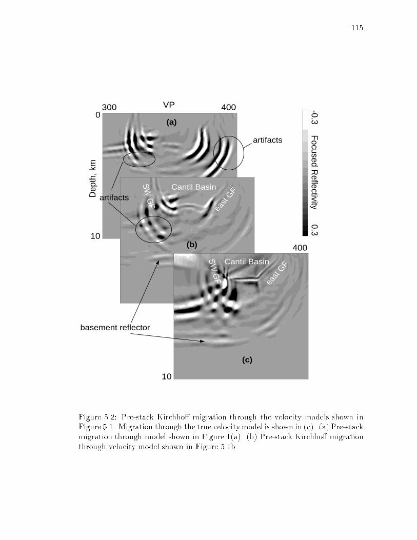
115

0

10

Dep

th, k

m

300 400VP -0.30.3

Focused Reflectivity

10

400

artifacts

artifacts

basement reflector

east

GF

east

GF

SW

GF

SW

GF

Cantil Basin

Cantil Basin

(a)

(b)

(c)

Figure 5.2: Pre-stack Kirchho� migration through the velocity models shown inFigure 5.1. Migration through the true velocitymodel is shown in (c). (a) Pre-stackmigration through model shown in Figure 1(a). (b) Pre-stack Kirchho� migrationthrough velocity model shown in Figure 5.1b.

116

5.5 Results Using Data From COCORP Line 1

First-arrival times (588 picks) and the raw-shot gather itself (Figure 3.19) recorded

along the southern segment of COCORP line 1 data (Figure 3.19) make up the data

for the combined optimization. The picking error is about 0.02 seconds. The model

is 13 km long and 8 km deep. Figure 5.3 shows the results of the optimization.

Comparing Figure 5.3a and 3.20c we see that including the coherency criteria

increases the depth of resolved velocities. Consequently, a pre-stack migration

through the model in Figure 5.3a images deeper re ectors (Figure 5.3c; compare

with Figure 3.22b). Low fold of the multi-o�set data leads to poor imaging on

the southwest side of the image. This side also shows larger standard deviations

(Figure 5.3b).

5.6 Results Using Data From COCORP Line 5

I pick �rst-arrival times o� 28 shot gathers recorded along COCORP Line 5 across

the Garlock fault in Cantil Valley, California (see Figure 4.7). A total of 611 travel-

time picks (picking error of 0.02 seconds) are used. The raw shot-gathers are used

in the re ection coherency calculation. Figure 5.4a shows the velocity model from

using only �rst-arrival travel times. Velocity resolution becomes poor below 1.5

km. A pre-stack migration through this model is shown in Figure 5.4a. Lack of

good velocity information below 1.5 km leads to poor focusing of coherent energy.

It is hard to discern any re ectors. Figure 5.4c shows the velocity model obtained

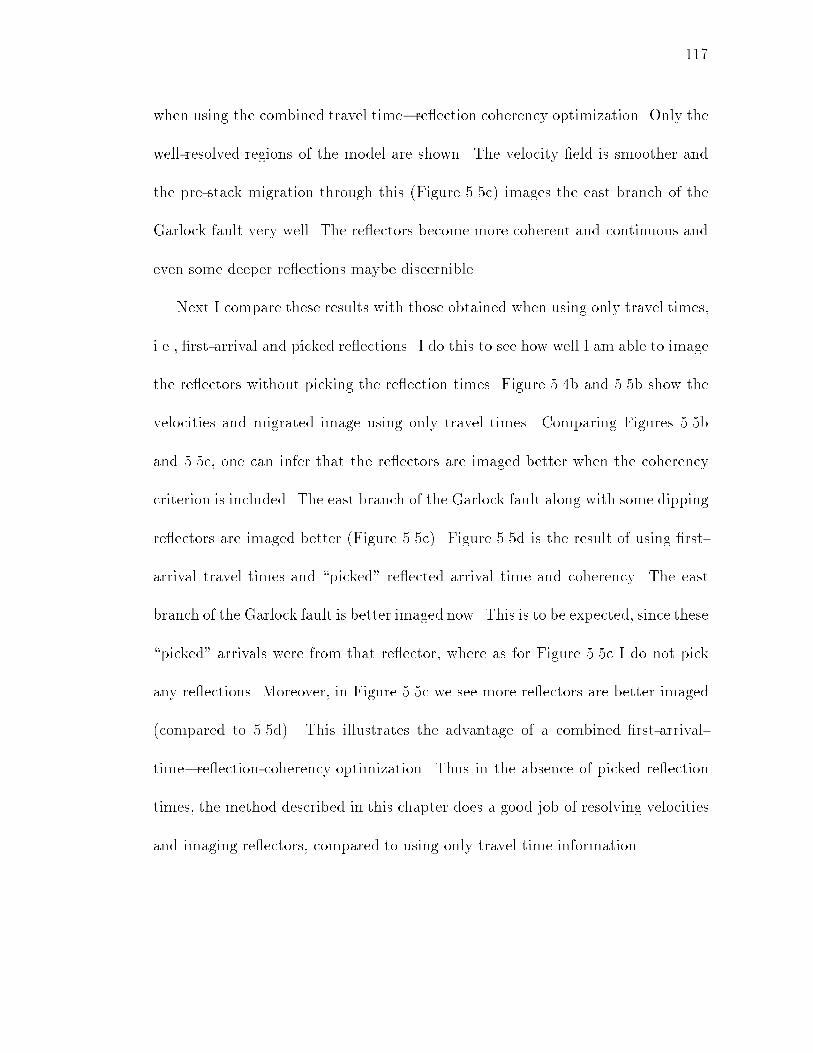
117

when using the combined travel time�re ection coherency optimization. Only the

well-resolved regions of the model are shown. The velocity �eld is smoother and

the pre-stack migration through this (Figure 5.5c) images the east branch of the

Garlock fault very well. The re ectors become more coherent and continuous and

even some deeper re ections maybe discernible.

Next I compare these results with those obtained when using only travel times,

i.e., �rst-arrival and picked re ections. I do this to see how well I am able to image

the re ectors without picking the re ection times. Figure 5.4b and 5.5b show the

velocities and migrated image using only travel times. Comparing Figures 5.5b

and 5.5c, one can infer that the re ectors are imaged better when the coherency

criterion is included. The east branch of the Garlock fault along with some dipping

re ectors are imaged better (Figure 5.5c). Figure 5.5d is the result of using �rst-

arrival travel times and \picked" re ected arrival time and coherency. The east

branch of the Garlock fault is better imaged now. This is to be expected, since these

\picked" arrivals were from that re ector, where as for Figure 5.5c I do not pick

any re ections. Moreover, in Figure 5.5c we see more re ectors are better imaged

(compared to 5.5d). This illustrates the advantage of a combined �rst-arrival-

time�re ection-coherency optimization. Thus in the absence of picked re ection

times, the method described in this chapter does a good job of resolving velocities

and imaging re ectors, compared to using only travel time information.

118

0

8

Dept

h, k

m

0 13Distance NE, km

CM-1 South Segment Velocity Optimization

0

6.5

Velo

city,

km

/sBasinSAFZ

0.55

0

8

Dept

h, k

m

CM-1 South Segment Standard Deviations

0

Velo

city

Rang

e, k

m/s

0

8

Dept

h, k

m

-0.4

0.4

Focu

sed

Refle

ctivi

ty

CM-1 South Segment Pre-stack Migration

SAFZ

Figure 5.3: Results of using the optimization scheme on COCORP Line 1 datacrossing the Mojave segment of the San Andreas fault. (a) and (b) shows theobtained velocity model and associated standard deviations. Regions below thedotted line are unconstrained. (c) Pre-stack migration through the model in (a).We are able to image deeper re ectors (compare with Figure 3.20.

119

5.7 Inferences

Results from synthetic and real data show that including the re ection coherency

criterion increases the depth of resolution of the obtained velocities. Consequently,

pre-stack migration through velocities obtained by this method image both shal-

low and deep re ectors. Comparisons of this approach, i.e., re ection coherency

maximization plus �rst-arrival time minimization, with re ection travel time plus

�rst-arrival time minimization, show that the former yields more robust results.

By doing a pre-stack migration, one can simultaneously image many re ectors. In

contrast, a travel-time-only inversion reconstructs just one. This method does not

involve any computations in addition to travel times. Hence it is computationally

comparable to the usual travel time inversion. Finally, the method does not require

picking of re ections, which makes it very attractive in areas such as fault zones

and continental margins where the complex geology causes the recorded data to

have complicated arrivals.

120

0D

epth

, km

238 383VP

1.675.1 Vel, km/s

1.5

0

Dep

th, k

m

4

0

5

Dep

th, k

m

sourcesreceivers

Cantil Basin

14.5 km

Cantil Basin

South North

(a)

(b)

(c)

Figure 5.4: Results of our optimizations using data recorded along the northernsegment of COCORP Line 5 crossing the Garlock fault in Cantil Valley, Califor-nia. Only the well-resolved regions are shown. (a) Velocity model by using only�rst-arrival travel times. Resolution becomes poor below 1.5 km. (b) Velocitymodel obtained after using re ection travel times in addition to �rst-arrival times.Velocities are well-resolved only down to 4 km. (c) Velocity estimate by using�rst-arrival travel times along with the re ection coherency criterion. This did notrequire picking re ection times, unlike (b).

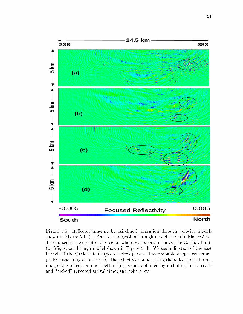
121

238 38314.5 km

5 km

(a)

5 km

(b)

5 km

(c)

-0.005 0.005Focused Reflectivity

South North

5 km

(d)

Figure 5.5: Re ector imaging by Kirchho� migration through velocity modelsshown in Figure 5.4. (a) Pre-stack migration through model shown in Figure 5.4a.The dotted circle denotes the region where we expect to image the Garlock fault.(b) Migration through model shown in Figure 5.4b. We see indication of the eastbranch of the Garlock fault (dotted circle), as well as probable deeper re ectors.(c) Pre-stack migration through the velocity obtained using the re ection criterion,images the re ectors much better. (d) Result obtained by including �rst-arrivalsand \picked" re ected arrival times and coherency.

122

Chapter 6

Conclusions and Suggestions

6.1 Summary

Obtaining velocity estimates and re ector characteristics in the earth's crust from

multi-o�set surface seismic data is the main goal of seismic data processing. This

work, in turn, is important for mineral exploration, geologic studies, and for un-

derstanding the tectonics of a region. Arrival times of di�erent phases on recorded

seismograms provide information about the velocities and re ectors. Inversion of

these times is one way of extracting this information.

Numerous such methods have been developed in the last decade. They have

evolved from using simple straight rays, to curved rays that account for lateral

velocity variations. However, most of these inversions su�er from the problem

of initial-model dependency Several constraints have to be included in the initial

model for the solution to be geologically viable (Stork, 1988). Previous studies

using least-squares velocity inversion (Santosa and Symes, 1988) have revealed

that the large eigenvalues associated with the travel time perturbations make the

iterativemethod very ine�cient. This thesis presents the use of a nonlinear, Monte-

123

Carlo optimization technique called simulated annealing that addresses these prob-

lems. This method is not dependent on any initial model, requires minimum a pri-

ori constraints, does not involve any matrix manipulations, and is computationally

tractable. The user has complete control over model perturbation, and use this

method to propose only reasonable models. In addition simulated annealing does

far better than inversion on seriously under-sampled (under-determined) data sets.

It will produce a reasonable model matching whatever data are available, where

any inversion method fails or produces serious artifacts. The absence of any matrix

computations makes this optimization scheme free of singularity, matrix stability,

and memory storage problems.

I develop an algorithm that can handle both �rst-arrival and re ection times.

Later this is extended to include amplitude information contained in the data. The

forward modeling, or the computation of travel times through velocity models, is

rapidly performed by a �nite-di�erence solution to the eikonal equation (Vidale,

1988). Vidale's original code computes any type of �rst arrival. This is modi�ed to

also compute re ected arrivals. The Monte-Carlo nature of the objective function

makes it easy to construct new objective functions and thus include new (di�erent

type) of data. The problem can be cast as having two totally separable objectives,

requiring only forward modeling for each data type. This would be hard to realize

in a standard inversion scheme.

The simulated-annealing algorithm works because it extensively samples the

model space. This property is put to use to estimate the uncertainty associated

124

with the \�nal" model parameters. As shown in Chapter 2, the fact that the prob-

ability of accepting new models is related to the posterior probability distribution

of the model parameters, we are justi�ed in using the models sampled during the

optimization for the uncertainty analysis. In all cases, I test the method using syn-

thetic data, compare it to a linearized inversion method, and apply it to real data

sets. Where applicable I discuss the tectonic implications based on the velocity

estimates and imaging results obtained from the data.

In Chapters 3 and 4 the nonlinear optimization method is compared with a lin-

earized least-squares method. The examples, both using �rst-arrival and re ection

times, show that annealing algorithm is not initial-model dependent. Moreover,

at the end of an optimization run, it produces a suite of models that have similar

least-square error. Thus, one can choose the velocity model that best suits the a

priori knowledge of the geology of a region.

Chapter 3 shows how the simulated-annealing algorithm can be used to obtain

well-resolved velocities in the shallow crust from �rst-arrival times. Results from

data collected in the Death Valley region of California indicate that these velocities

can be used to delineate shapes of basins and estimate the nature of faulting. These

results, coupled with geologic and other seismic evidence provide some constraints

on the nature of Cenozoic extension in the region. Another use of accurately-

estimated velocities is shown by using the velocities in a pre-stack migration, and

imaging faults directly from their re ections. It is important to use a method that

can recover rapid lateral changes in velocities because faults are often associated

125

with such velocity changes. It also presents the user with the ability to perform

the migration in the shot-receiver space, the domain in which the data is recorded.

Poor lateral velocity resolution would have meant that the migration be performed

in the midpoint-o�set space (a transformation) as suggested by Claerbout (1998)

to minimize migration errors. By avoiding that, we preserve the angle accuracy

and avoid spatial aliasing when the shots are far apart. Examples of imaging the

o�shore Hosgri fault and the Mojave segment of the San Andreas fault in California

demonstrate the e�ectiveness of this approach. The fault images were corrupted

and incoherent before the velocity models were resolved well. Direct imaging of

the fault plane helps de�ne the subsurface geometry of a fault and its relationship

with adjoining truncated beds (as shown for the Hosgri fault). Thus, the combined

use of optimization for velocities and pre-stack migration helped in understanding

the tectonic framework of two regions.

Re ection times depend on both velocities and re ector depths. This makes

inversion of these times a nonlinear process. Chapter 5 shows how well-suited the

simulated-annealing method is to handling this problem. Use of re ection times

is a more direct way to simultaneously obtain velocities and subsurface geometry

of re ectors. They sample deeper horizons than �rst arrivals and can reconstruct

re ector depth, length, and dip. The Garlock fault example shows the e�ectiveness

of this method on real data. Comparisons with results of Louie an Qin (1991), re-

veal that the reconstructed re ector agrees well with a pre-stack migration through

the velocity model. Thus with minimum a priori assumptions one is able to obtain

126

detailed information about subsurface structures. I also show that including more

information contained in the data signi�cantly improves the results. Speci�cally, I

constrain the upper 1.0 km using �rst-arrival picked o� the shot gathers. Now, I'm

able to obtain well-resolved velocities down to 5 km and reconstruct the re ector

to almost the surface (Figure 4.12). The main drawback of this method is that

the re ection travel times, which are the input to the optimization scheme, need

to be picked. This could be a di�cult proposition in areas where the recorded

seismograms are complicated due to the geology underlying the region.

Chapter 5 presents solutions to two problems that are often encountered when

inverting re ection times. The �rst is the resolution of re ector depth�velocity

ambiguity. This is addressed by including more information from the data, namely

the amplitudes of re ected arrivals. The second problem is picking re ection times

from recorded seismograms. A solution to this involves picking only the �rst ar-

rivals, which is easily done, and using a \coherency" measure of the re ections.

The �rst-arrival travel times constrain velocities at shallow depths, while re ec-

tion coherency provides information from deeper horizons. The exibility of the

simulated-annealing algorithm allows for simultaneously solving both problems.

A pre-stack migration through the �nal velocity model images the re ectors.

Results from synthetic examples and using COCORP lines 1 and 5 from the Mojave

Desert of southern California show the method's ability to resolve velocities deeper

than when using only �rst-arrival times. In addition, pre-stack migrations through

these velocities produce more coherent images of re ectors. Lastly, this scheme

127

produces results equivalent to an iterative pre-stack migration, a commonly used

interpretation tool, but has the advantage of being computationally less expensive.

The main drawback of using this nonlinear optimization scheme is that the

method becomes computationally expensive when the number of model parameters

being estimated becomes very large (around 10,000 or more). I suggest some

remedies for this in the next section.

6.2 Suggestions

Use of the nonlinear optimization gives us solutions despite having very little a

priori knowledge, while a linearized inversion is initial-model dependent. This

suggests that the models obtained by the optimization method developed in this

thesis can used as input to a linearized inversion. This was tried, but did not

always provide better results. I think such an approach will be e�ective only when

inverting for just the velocities. The linearized inversion does not do well when

the re ector is allowed to vary by much.

For most of the problems, I perform simulated-annealing runs using di�erent

initial models. It would be worthwhile to do the same using di�erent random num-

ber seeds. This will probably force the algorithm to sample di�erent parts of the

model-space, and many such runs could help de�ne the null-space of the problem.

Using models from all these di�erent annealing runs in the statistical analysis, for

determining the model-parameter uncertainties, should give more robust results.

128

A natural extension of the method described will be to three dimensions. The

forward modelling will be accomplished by a �nite-di�erence solution to the eikonal

equation in three dimensions (Vidale, 1990; Hole et al., 1992). Optimization in

three dimensions will make the approach amenable to estimating velocities using

regional earthquake data. Some work has been done in this direction. Such a

method was used to estimate velocities and hypocenter locations from aftershocks

of the March 17, 1993, Eureka Valley earthquake recorded by portable stations

deployed by the University of Nevada, Reno (Asad et al., 1994). The optimization

is performed simultaneously for velocity, hypocenter, and origin time. In this case

velocity results seem more robust than those from linearized methods, due to the

advantages of optimization for data sets having poor coverage. The main problem

encountered in these optimizations seem to be with the hypocenter locations. Their

locations did not match well with those from linear methods. Further work needs

to be done to investigate if including constraints like requiring all the hypocenters

to lie in a plane, putting limits on their depths, or allowing only small depth

perturbations at each iteration will improve the optimization results.

Regional velocities are determined from earthquake data usually by performing

a joint hypocenter-velocity inversion, or from travel time data picked from seismic-

refraction surveys. Simulated annealing in three dimensions o�ers the opportunity

to use both types of data sets simultaneously. While earthquakes, with their

relatively broad depth coverage, provide control on vertical velocity variations,

surface data help constrain velocity variations in the horizontal direction. The

129

objective function is formulated similarly to the \coherency" problem in Chapter

5. Thus I was able to combine data sets having very di�erent scales. This is

approach is applied to get three-dimensional velocities in and around the pull-

apart basin formed by the two segments of the Garlock fault meeting in Fremont

Valley, California (Pullammanappallil et al., 1994). Once again, the hypocenter

relocation by this process needs further work. An extension of this work would

be include re ection travel times or gravity data in the optimization. These o�er

a attractive ways to estimate regional velocities in and around faults which are

seismically active and have a surface seismic survey completed nearby.

The nature of implementation of the simulated-annealing algorithm makes is

conducive for parallel programming. Forward modeling through models perturbed

di�erently can be performed on di�erent machines simultaneously. This would

be done for a �xed temperature. These models will be compared and one model

accepted based on the computed conditional probabilities. Then, this model will

form the basis for annealing at the next lower temperature. Thus, one can do the

forward modeling in parallel and speed up the optimization process.