computing the envelope for stepwise constant resource ... · computing the envelope for stepwise...
TRANSCRIPT

Computing the envelope for stepwise constant resource allocations
Nicola Muscettola
NASA Ames Research Center
Moffett Field, California 94035
Abstract
Estimating tight resource level bourds is a fundamentalproblem in the construction of flexibl _plans with resourceutilization. In this paper we describe an efficient algorithmthat builds a resource envelope, the rightest possible suchbound. The algorithm is based (,n transforming thetemporal network of resource consuming and producingevents into a flow network with node; equal to the eventsand edges equal to the necessary pred{_cessor links betweenevents. The incremental solution of a staged maximumflow problem on the network is then used to compute thetime of occmTence and the height of each step of theresource envelope profile. The staged algorithm has thesame computational complexity of solxing a maximum flowproblem on the entire flow network. This makes thismethod computationally feasible for use in the inner loopof search-based scheduling algorithms.
Introduction
Retaining flexibility in the execution of activity plans is afundamental technique for dealing with the uncertainconditions under which the plans will be executed. Forexample, flexible plans allow explici: reasoning about thetemporal uncontrollability of exogenous events (Morris,Muscettola, Vidal 2001) and tl_e incorporation ofexecution countermeasures within the flexible network•
Tightly constrained schedules (e.g., ;,chedules that assigna precise start and end time to all activities) are typicallybrittle and it is very difficult to closely follow theirdirections during execution. For an example of whatoverly tight schedules can do to an intelligent executionsystem, consider the "Skylab strike" (Cooper, 1996), whenduring the Skylab 4 mission astronau:s went on a sit-downstrike after 45 days of trying to catch up with the demandsof a fast paced schedule with no roorc fi_r them to adjust tothe space environment.A major obstacle to building flexible schedules, however,remains the difficulty of accurately es,timating the amountof resources that a flexible plan may need across all of itspossible executions. This problem is particularly difficultfor resources with multiple capacity' that can be bothconsumed and produced. In the worst case large plans mayexhibit both a high level of activity p_ rallelism and a largenumber of required synchronizatior constraints amongactivities. Most of the scheduling rmthods available todate for this problem (Cesta, Oddi Smith, 2000) eventuallyproduce a fixed activity schedule, even if they makesubstantial use of an activity plan s flexibility duringschedule construction.
To appreciate the difficulty of precisely estimatingresource consumption, consider the fact that a flexibleactivity plan has an exponential mmber of possible
instantiated schedules. This means that methods based on
complete enumeration are typically out of the question.Lately, however, new techniques have been developedCLaborie, 2001) based on direct propagation ofinformation on the temporal constraints of the plan. Thisyields both an upper bound and a lower bound on theresource level required by the plan over time. Thisinformation can be used in various ways, e.g., to decidewhen to backtrack (when the lower/upper bound intervalis outside of the range of allowed resource levels at sometime) and when a solution has been achieved (when thelower/upper bound interval is inside the range of allowedresource levels at all times). Bound tightness is extremelyimportant computationally since both as backtracking andtermination criteria it can save a potentially exponentialamount of search when compared to a looser bound.A natural question is whether constructing the tightestpossible resource level bounds is computationally feasible.This paper answers this question in the affirmative. Wedescribe an efficient algorithm for the computation of aresource level envelope, a resource level bound such thatfor each time there exists at least a schedule for the
activity plan that will consume the amount of resourceindicated by the bound. The algorithm is polynomial, withcomplexity equivalent to solving a maximum flowproblem on a flow network of the size of the originalactivity plan.In the rest of the paper we first introduce the formal modelof activity networks with resource consumption. Then wereview the literature on resource contention measures and
show an example in which the current state of the art inresource level bounds is inadequate. Then we give anintuitive
resourcebetweenacti vitiesresourceactivitiesefficientconclude
understanding of our method to compute theenvelope. Then we establish the connectionmaximum flow problems and finding sets ofthat have the optimal contribution to the
envelope. We then show that these sets ofcompute an envelope. We then describe anenvelope algorithm and its complexity. Wediscussing future work.
Activity Networks and Resource Consumption
Figure l shows an activity network with resourceallocations. The network has two time variables peractivity, a start event and an end event (e.g., ex_ and e_ foractivity AI), a non-negative flexible activity duration link(e.g., [2, 5] for activity A1), and flexible separation linksbetween events (e.g., [0, 4] from e3, to e40. A time origin,Ts, corresponds to time 0 and supports separation links toother events. We assume that all events occur after T_ and
https://ntrs.nasa.gov/search.jsp?R=20020052599 2018-07-28T22:49:05+00:00Z

before an event Te rigidly connected to Ts. The interval
TsTe is the time horizon T of the ne work.
<e2,. r>> [2.3] <e___, rz__>
<e_. r.> [2.5] <elc.-rl>/I A: \
?/ A' ,_2. 3]_k4. 0'6] <e.,_. r,> [0, +_J
/ E,,,ol....j
/[1, 41 _'_m_m_V---. _ r0, +oofi
j <e,,,r,,>A, <o.,r.>T, [30, 30] T:
r, • [ 1, 4] r:,_ • i-7,-5]
r_l_ [-I,3j r:_:• 1, 3]
r22• [I,2) r_ c 2, a]
Figure 1: An activity network with re._;ource allocations.
Time origin, events and links constitute a' SimpleTemporal Network (STN) (Dechter, Meiri, Pearl 1991).
Unlike :regular STNs, however, each event has an
associated allocation variable with real domain (e.g., ral
for event ea_) representing the amount of resource
allocated when the event occurs We will caIl this
augmented network R a piecewi_;e-constant Resource
allocation STN (cR-STN). In the following we will assume
that all allocations refer to a single, multi-capacityresource. The extension of the results to the case of
multiple resources is straightforward An event e with
negative allocation is a consumer, while an e + with
positive allocation is a producer.
Note that an event can be either a ccnsumer or a producer
in different instantiations of the allo:ation variables (e.g.,
event ez_ for which the bound for r2_ is [-1, 3]). This
allows reasoning about dual-use activities (e.g., starting a
car and running it both make use of the alternator as a
power consumer or producer). Moreover, some events can
have opposite resource allocation of Xher events (e.g., e_
vs. e_,). This allows modeling reusab e allocations, such as
power consumption by an activity. ',Iote that this model
does not cover continuous accumulat on such as change of
energy stored in a battery over t:me. A conservative
approximation can however be achieved by accounting for
the entire resource usage at the activity start or end. We
will always assume that the cR-STN is temporally
consistent. From the STN theory, this means that the
shortest-path problem associated te R has a solution.
Given two events ex and ez we ¬e with le_e, I the
shortest-path from e_ to e> We will call a full instantiation
of the time variables in R a schedule s(.) where s(e) is the
time of occurrence of event e accordi:lg to schedule s. We
will call S the set of all possible corsistent schedules for
R. Each event e has a time bound [el(e), It(e)], with et(e)= -leT_l and It(e)= ITse], representing the range of time
values s(e) for all s_ S. Finally, give1 three events, ea, ez
and ea, the triangular inequality le,eal -< I<e,_l + ]e2ealholds.
A fundamental data structure used in the rest of the paper
is the precedence graph, Pred(R), fcr a cR-STN R. This
is defined as a graph with the same events as R and such
that for any two events el and e2 with le_ e2l -< 0 there is a
path fiom et to e., in Pred(R). Alternatively, we can say
that an event e_ precedes another ez in the precedence
gaph if e_ cannot be executed before e2. There are several
possible precedence graphs for a network R, A way to
build one is to run an all-pairs shortest-path algorithm and
retain only the edges with non-positive shortest distance.
Smaller graphs can be obtained by eliminating dominated
edges, e.g., by applying dispatchability minimization
(Tsamardinos, Muscettola, Morris 1998). The cost of
computing Pred(R) is bound by O(VE + V z lg V) where
V is the number of events and E the number of temporal
distance constraints in the original cR-STN. The use of
different precedence graphs may affect algorithm
performance but does not affect the theoretical foundationdescribed here.
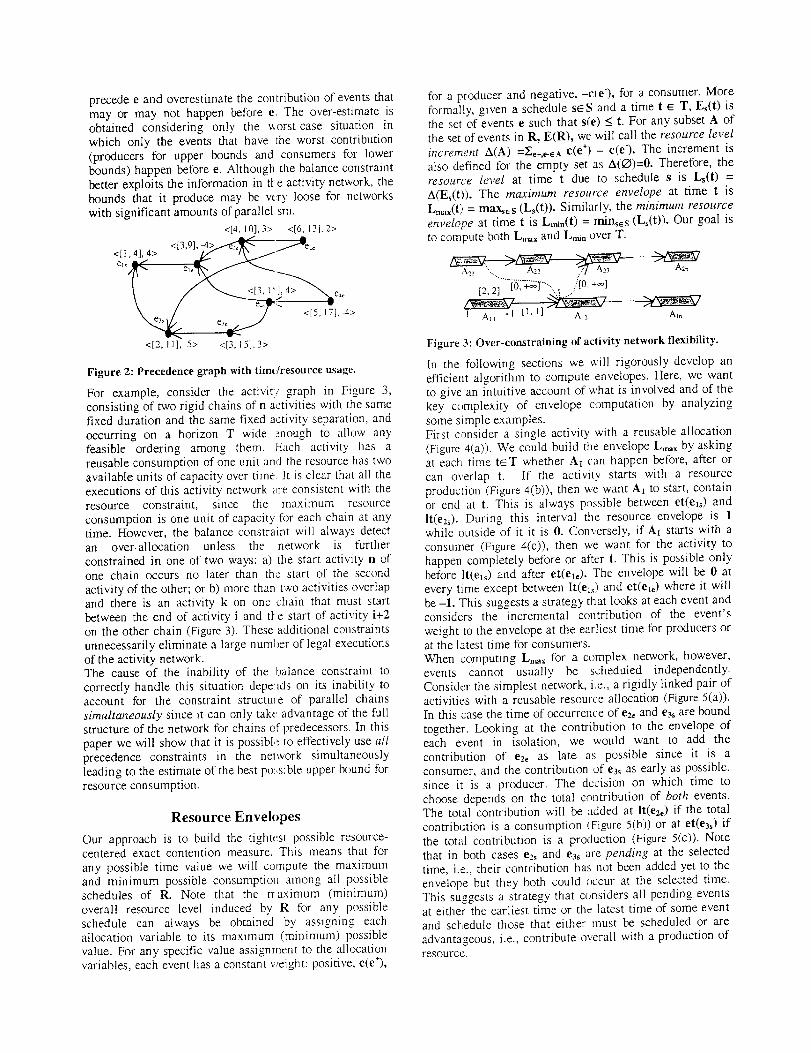
Considering again the activity network in Figure 1, Figure
2 depicts one of its precedence graphs with each eventlabeled with the time bound and the maximum allowed
resource allocation.
Resource Contention Measures
Safe execution of a flexible activity networks needs to
avoid resource contention, i.e., the possibility that for
some o.msistent time assignment to the events there is atleast one time at which the total amount of resource
allocated is outside the availability bounds. There are
essentially two methods tbr estimating resourcecontention: heuristic and exact. Most of the heuristic
techniques (Sadeh, 1991)(Muscettola, 1994)(Beck et al.,
1997) measure the probability of an activity requesting a
resource at a certain time. This probability is estimated
either analyticaIIy on a relaxed constraint network or
stochastically by sampling time assignments on the full
constraint network. The occurrence probabilities are then
combined in an aggregate demand on resources over time,
the contention measure. Probabilistic contention can give
a measure of likelihood of a conflict occurring. However,
it is not a safe measure, i.e., the fact that it does not
identify any conflict does not exclude the possibility thatthe cR-STN could have a variable instantiation with
inconsistent resource allocation. Exact methods avoid this
problem and are based on the computation of sufficient
conditions for the lack of contention. (Laborie, 2001) has a
good survey of such methods. Current exact methods
operate on relaxations of the full constraint network. For
example, edge-finding techniques (Nuijten, 1994) analyze
how an activity can be scheduled relatively to a subset of
activities, comparing the sum of all durations with a timeinterval derived from the time bounds of all the activities
under consideration. Relying only, on time bounds ignores
much of the inter-activity flexible constraints and tend to
be effective only when the time bounds are relatively tight.
Therefore algorithms that use these contention measures
tend to eliminate much of the flexibility in the activity
network. (Laborie, 2001) goes further in exploiting the
information about mutual activity, constraints. One of the
two metrics proposed in that paper is the balance
constraint, an event-centered approach that estimates
upper and lower bounds on the resource level immediatelybefore and after each event e in the cR-STN. These bounds
precisely estimate the contribution of events that must
precedeeandoverestimatethecontributionofeventsthatmayor maynothappenbeforee. The over-estimate is
obtained considering only the ,aorst-case situation in
which only the events that have the worst contribution
(producers for upper bounds and consumers for lower
bounds) happen before e. Although the balance constraint
better exploits the information in t/-e activity network, the
bounds that it produce may be very loose for networks
with significant amounts of parallel sin.
<[4, 10],3> <[6, 13j, 2>
<[3 9]-4>_k/_--_TC;;:J e<1,4; 4> ' "Z W_', _ ;_
e__y <[5, 17]. 4>
<[-2, I 1l, -5> </3, 15]. 3>
Figure 2: Precedence graph with tim_/resou rce usage.
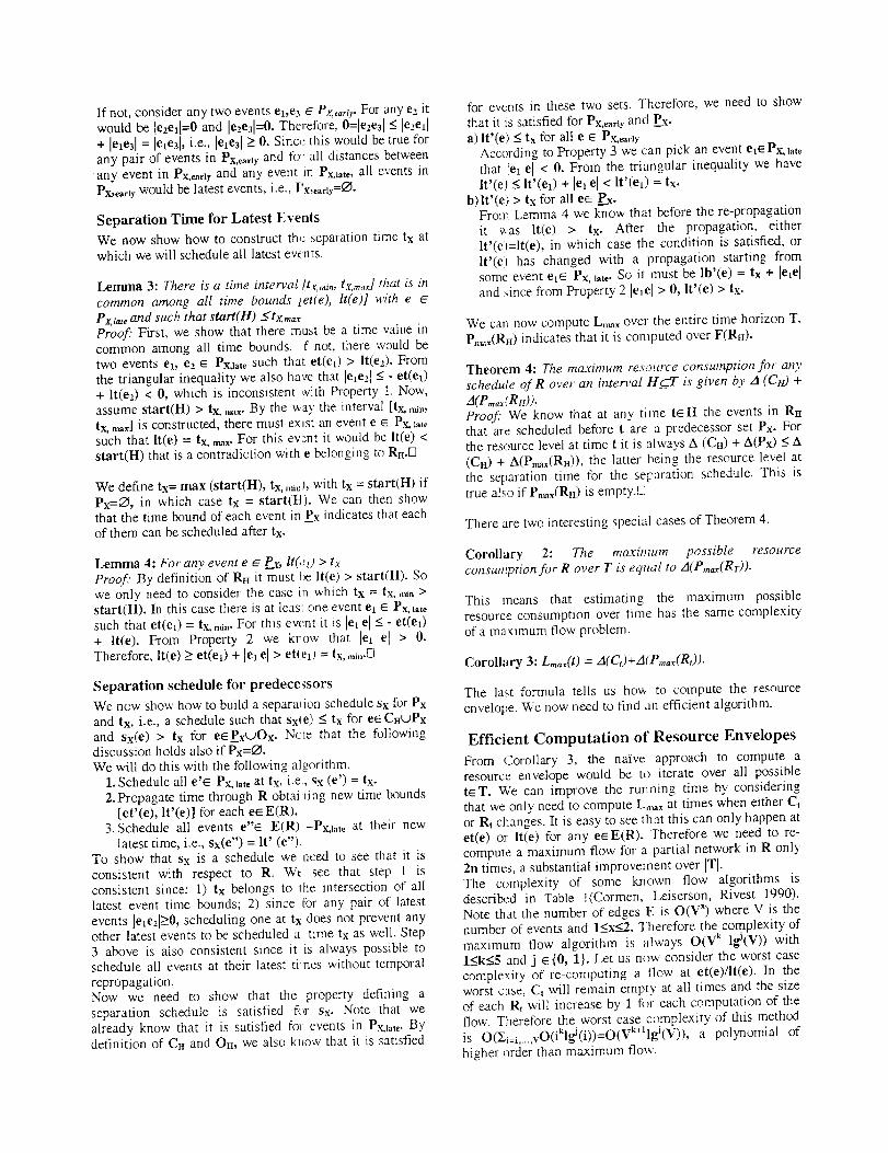
For example, consider the activir: graph in Figure 3,
consisting of two rigid chains of n activities with the same
fixed duration and the same fixed activity separation, and
occurring on a horizon T wide _nough to allow any
feasible ordering among them. Each activity has a
reusable consumption of one unit and the resource has two
available units of capacity over time It is clear that all the
executions of this activity network _Ire consistent with the
resource constraint, since the maximum resource
consumption is one unit of capacity for each chain at any
time. However, the balance constraint will always detectan over-allocation unless the network is further
constrained in one of two ways: a) the start activity n ofone chain occurs no later than the start of the second
activity of the other; or b) more than two activities overlap
and there is an activity k on one chain that must start
between the end of activity i and tte start of activity i+2
on the other chain (Figure 3). These additional constraints
unnecessarily eliminate a large num1_er of legal executions
of the activity network.
The cause of the inability of the balance constraint to
correctly handle this situation depe ids on its inabitity to
account for the constraint structure of parallel chains
simultaneously since it can only take: advantage of the full
structure of the network for chains of predecessors. In this
paper we will show that it is possibL' to effectively use all
precedence constraints in the nelwork simultaneously
leading to the estimate of the best po:,sible upper bound for
resource consumption.
Resource Envelopes
Our approach is to build the tightest possible resource-centered exact contention measure. This means that for
any possible time value we will compute the maximum
and minimum possible consumptio_ among all possible
schedules of R. Note that the rraximum (minimum)
overall resource level induced by R for any possible
schedule can always be obtained by assigning each
allocation variable to its maximum (minimum) possible
value. For any specific value assigmnent to the allocation
variables, each event has a constant weight: positive, e(e*),
for a producer and negative, -c(e), for a consumer. More
formally, given a schedule seS and a time t • T, E_(t) is
the set of events e such that s(e) _< t. For any subset A of
the set of events in R, E(R), we will call the resource level
increment A(A) =£ ..... _A c(e+) - c(e). The increment is
also defined for the empty set as A(O)=0. Therefore, the
resource level at time t due to schedule s is Ls(t) =
A(E_(t)). The maximum resource envelope at time t is
L,,_=(t) = ma-N_s (L._(t)). Similarly, the minimum resource
envelope at time t is L,,_,(t) = min_s (L,(t)). Our goal is
to compute both L,,_ and L,,i, over T.
A2..
-, ............7= ..........:, ....../,
Figure 3: Over-constraining of activity network flexibility.
In the following sections we will rigorously develop an
efficient algorithm to compute envelopes. Here, we want
to give an intuitive account of what is involved and of the
key complexity of envelope computation by analyzing
some simple examples.
First consider a single activity with a reusable allocation
(Figure 4(a)). We could build the envelope L,_. by asking
at each time teT whether A_ can happen before, after or
can overlap t. If the activity starts with a resource
production (Figure 4(b)), then we want A_ to start, contain
or end at t. This is always possible between et(e_s) and
lt(%_). During this interval the resource envelope is 1
while outside of it it is 0. Conversely, if A1 starts with a
consumer (Figure 4(c)), then we want for the activity to
happen completely before or after t. This is possible only
before lt(el_) and after et(el_). The envelope will be 0 at
every time except between It(eta) and et(el_) where it will
be -1. This suggests a strategy that looks at each event and
considers the incremental contribution of the event's
weight to the envelope at the earliest time for producers orat the latest time for consumers.
When computing L,,,, for a complex network, however,
events cannot usually be scheduled independently.
Consider the simplest network, i.e., a rigidly linked pair of
activities with a reusable resource allocation (Figure 5(a)).
In this case the time of occurrence of e2_ and e._ are bound
together. Looking at the contribution to the envelope of
each event in isolation, we would want to add the
contribution of e2, as late as possible since it is a
consumer, and the contribution of e3s as early as possible,
since it is a producer. The decision on which time to
choose depends on the total contribution of both events.
The total contribution will be added at lt(e2_) if the total
contribution is a consumption (Figure 5(b)) or at et(e3_) if
the total contribution is a production (Figure 5(c)). Note
that in both cases e2_ and e,_ are pending at the selected
time, i.e., their contribution has not been added yet to the
envelope but they both could occur at the selected time.
This suggests a strategy that considers all pending eventsat either the earliest time or the latest time of some event
and schedule those that either must be scheduled or are
advantageous, i.e., contribute overall with a production of
resource.

Nowconsiderthenetworkin Figulel andtheeventtimebounds,maximumresourceallocationandprecedencegraphin Figure2. Assumethatwewantto computeL,mx(3), the maximum envelope at time 3. The set of
events that may be scheduled before, at or after time 3 is
{el_, exe, e3s, %o e4s}. However, of hese only {ele, e3s, e3e,
e4_} are pending since it is advanta;.,eous to consider el_ atits earliest time 1. The subset of events that we could
consider at time 3 are all those that will have to occur at or
before 3 assuming that we select fcr some set of events to
occur at 3. These subsets are {e3,}, {el_}, {e3e, e3s} and {e4_,
exe, eae, eas}. Unfortunately, each )f these subsets has a
negative weight and therefore none of them is considered
at time 3. At time 4 the set :)f pending events is
augmented with ezs and the total c )ntribution of the new
subset of pending events {e2,, e4s, e>, e3_, e3s} is positive.
<[0.31, r_> <[5, t0], n>
els AI eje
(a)
1
i[o_.-
(b) ,c)
Figure 4: Maximum resource envelnp_, for a single activity.
The selection of a maximally advar tageous subset among
the pending events is the key source of complexity ofenvelope calculation. An exhaustive enumeration of all
subsets can obviously be very expensive. Fortunately we
can make very good use of the information in the
precedence _aph. It turns out _hat this problem is
equivalent to a maximum flow p oblem solved on an
appropriate auxiliary flow network built on the basis of
Pred(R). We will discuss this rigor(,usly in the rest of the
paper.
Calculating Maximum Resource
Level Increme ats
Consider now an interval H_cT. We can partition aJ1
events in R into three sets depencing on their relative
position with respect to H: 1) the closed events Cn with
all events that must occur strictly before or at the start of
H, i.e., such that that It(e) <_ start(H); 2) the pending
events Ra with all events that can occur within or at the
end of interval H, i.e., such that It(e _ > start(H) and et(e)
< end(H); and 3) the open events Oa with all events that
must occur strictly after H, i.e., such that et(e) > end(H).
The set Rn could contain events tidal can be scheduled
both inside and outside H. If H=T, then CT= _, RT =
E(R) and On=O. The interval H could be reduced to a
single instant of time, i.e., H=[t, t] In this case we will
use the simplifying notation Ct=((ft, tl, Rt=Rtt. tl and
Ot=O[t, tl-
We are interested in a particular kind of subset of Rn.
Assume that we wanted to compu e the resource level
increment for a schedule s at a time t_ H. This will always
include the contribution of all evenv_ in Ca and none of
those in On irrespective of s and t. With respect to the
events in Rm we can see that if an event is scheduled to
occur at or before t then all of its predecessors (accordingto Pred(R)) will also have to occur at or before t. In other
words, it is possible to find a set of events X ff Rn such
that the events ep_RR that are scheduled no later than t in
s are those such that lexepl _< 0 for some e_ E X. We call
this the predecessor set of X, Px. Therefore, the resource
level at time t for a given schedule s is the sum of the
weights of events in Cn and in Px.
<[0,3],rl> <[4,10],-rl> <[5, ll],r2><[N, 14],-r2>
e2_ A, e2¢ [1, l] e._, As e3.
(a)
(b) (c)
Figure 5: Maximum envelope for two chained activities.
It is easy to verify that given two predecessor sets Px and
Py, both Px _ Pv and Px uPv are also predecessor sets.
Resource Level Increments and Maximum Flow
Since we are interested in the maximum resource level we
want to find the predecessor set with maximum resource
level increment. We will do so by finding a maximum
flow for an auxiliary flow network built from Ru and
Pred(R).
Resource Increment Flow Problem: Given a set of
pending events R_i for a cR-STN R, we define the resource
increment flow problem F(RH) with source o'and sink ras
follows:1. For each event e E RH there is a corresponding node
e cF(Rn).
2. For each event e + _Ru, there is an edge cr---) e ÷ with
capaci_ c(e+).
3. For each event e- E R_, there is an edge e---)'t" with
capaci_ c(e), i.e., the opposite of e-'s weight in R .
4. For each pair of e_ and e2 with an edge el--pe2 in the
precedence graph Pred(R), there is a corresponding
link el--Pe 2 in F(Rn) with capacity +oo,
................................;:::::::::::::::::::":::.iiiiill..............,,---..-..,:........
/ ........ \ +c%..-,.ff711"_ _ "".. "...
/ e,v-., _- / _ _"-.. "..'..
t_ & e'°I>-..-'_ _ ............)'::::.,t_. 5 _ +_/..,/'x,..._ . _ ..... :ps
"-,, / ,x ....../",.., ",,\ J_.'_Z.3 ..............
"-..'"------'>K_-- _....---÷_ ,./ ......"_" --.. _ e ;_7" 1-"1 .Y'
a---.. ...................................Internal flow (precedence constraints)
................... Incoming flow (producer events)
.... Outgoing flow (consumer events)
Figure 6: Resource increment flow problem.

As an example, Figure 6 shows the auxiliary flow problemfor RT relative to the activity network: in Figure 1.A detailed discussion of flow problems is beyond the scopeof this paper (for a complete treatment see (Cormen,Leiserson, Rivest 1990). Here we highlight somefundamental concepts and relations that we will use. Wewill indicate as f(el, ez) the flow associated to a linkev--+e2 in F(Ra). The flow functicn is skew-symmetric,i,e., f(e2, el) = - f(eu e2). Each flow has to be not greaterthan tbe capacity of the link to which it is associated. Forexample, referring to the flow netwcrk in Figure 6, 0 _<f(o',
e2e) < 2, 0 -< t'(eae, x) _<4 and f(e4_ e40 > 0. Note that aflow from el to e., can be negative only if the flow networkcontains an edge e2--+ea with posit.ve capacity. We alsouse an implicit summation notation f(A, B), where B andA are disjoint event sets in F(RH), te indicate the flow f(A,B) = £a_aZbGnf(a, b). Consider now any subset of eventsACRn and let us call A_A.the set of events A = RH-A. Thefollowing flow balance constraint always holds: f({o'}, A)= f(A, {'r} ) + f(A, A). The total netu ork flow is defined asf({o'}, RI0 = f(Rn, {z}). The maximum flow of a networkis a function f,,,,_ such that the t:)taI network flow ismaximum.
The fundamental concept used by all known maximumflow algorithms is the residual network. This is a flownetwork with an edge for each pair ff nodes in F(RH) forwhich the residual capacity, i.e., t[_e difference betweenedge capacity and flow, is positiw'. Each edge in theresidual network has capacity ecual to the residualcapacity. For example, considering he network in Figure6, assume that f(e_, _) = 3 and fro, e.,_) = 2. The residualnetwork for that flow will have the ]owing edges: e_--_zwith capacity 1, '_-+ele with capacizy 3 and e2e--ro withcapacity 2. Also note that any residual network for anyflow of F(R_0 will always have an edge of infinite capacityfor each edge in the precedence _aph Pred(R).In this paper we will make use of three different kinds ofpaths in the residual network. The f rst is an augmentingpath connecting cr to "_. The existence of an augmentingpath indicates that additional flow c m be pushed from crto x. Several maximum flow al[orithms operate bysearching for augmenting paths. Alternatively, the lack ofan augmenting path is the condition that indicates that aflow is a maximum flow. The second kind of path is aflow-shifting path, a loop connecting r to z which does notaffect the overall flow in the netwo: k. Finally, the thirdkind is a reducing path, i.e., a path _'om x to a. Pushingflow through a reducing path reduces a network's flow.We now establish the relation between the resource level
increment A(A) and any flow in F, Rr0. We define theproducer weight in A as c(A +) = Z_÷ e A c(e ÷) and theconsumer weight in A as e(A) = Y__e A e(e-). We alsodefine the producer residual in A as r(A +) = c(A ÷) -
f({a}, A), i.e., the total residual capacity of the edgeincoming A from s, and the consumer residual in A asr(A') = e(A) - f(A, {'_}). The followir g relation holds.
Lemma 1: A(A) = r(A +) - r(A') + f(A, A).Proof.. A(A) = e(A') - e(A) = (c(h +) - f({cr}, A)) - (c (A) - f(fcr}, A)) = r(h +) - (c(A) - f(a, {'c}) - f(A, _) =r(A +) - r(A) + f(A, A.A).[]
We now focus on predecessor sets such as Px.
Lenuna 2: f(Px, P_x) -_ O. Moreover, f(Px, Lt)=O if andonly if f(el, e2)=O for each el ff_v and e2ffPx.Proof." From the definition of predecessor there is no edgeez_el in F(Rn) with e_P_P.x and e2ePx. Therefore, f(e2,el) _< 0 and f(Px, P_P_x)-< 0. The second condition can bedemonstrated by observing that the sum of any number ofnon-positive numbers is 0 if and only if each number is 0._3
Another way to express Lemma 2 is that f(Px, P_x)=0 ifand onIy if there is no link el--+e2 in the residual networkwhere ele P_xand e:_ Px.
Corollary 1: A(Px) -<r(Px ÷) - r(Px ).Proof" [mmediate from Lemma I and Lemma 2.
IVlaximum flows and maximum resource level
increments
We are now ready to find the maximum positive resourcelevel increment. Note that we are not interested in event
sets with negative resource increments since; as wediscussed before, we will only account for events in ourresource envelope simulation if they have a positivecontribution. If they do not, we will take them into accountwhen we must, i.e., when their temporal upper boundbecomes lower or equal to the current simulation time.First we address the problem of whether Ru contains a setof predecessors P* with positive resource level increment,i.e., A(P*) > 0. To do so we will make use of a maximumflow f_,, of F(Ru). We will indicate with r,,_,x(A)producer/consumer residual computed for f,,,,,,. Thefollowing fundamental theorem holds.
Theorem 1: Given a partial plan Rm there is apredecessor set P* such that A(P*)>O if and only ifr,,_(RH +) > O.Proof [7 : We prove that if there is a P" such that A(P*)>0, then r ..... (RH +) > 0. Assume that r,_(Ra ÷) = 0. Thismeans that for any predecessors subset Px we haver,,_,(Px _) = 0. From Lemma 2 we would have A(P*) <-r,,_(P*) _<0, that is a contradiction.e=: We prove that if rn=_(Rn ÷) > 0 then we can identify aP" such that A(P')>0. If rn_(Rn +) is positive, there mustbe some e +such that r,,,,(e +) > 0. Let's select P" as the setof events reachable by some path in the residual networkoriginating from e +. The following three properties hold.1. P. is a predecessor set.
If not, there will be an event e: _ P* such that Me21 -<0for some event e_eP*. From the definition of Pred(R),
however, we know that there must be a path in Pred(R)from el to e2. Since this path will be present in F(RH)with all links having infinite capacity, the path will alsoalways be present in any residual network for any flow.Therefore there is a path in the residual network goingfrom e+ to e_ to e2 and e2_P*, which is a contradiction.
2. r,,_(P *) = O.If not, there will be an event e _ P* such that ru,a_(e) >
0. We can therefore build an augmenting path of F(RH)as follows: i) an edge o'--+e* with positive residualcapacity r,,,a_(e+); 2) a path in the residual network from

e+toe, whichexistsbydefinitio_ofP";and3)anedgee--_'_withresidualcapacityr=m(e).Theexistenceoftheaugmentingpathmeansthatf,,,_isnotamaximumflow,whichisacontradiction.
3.f,=.o'; £3 = 0Since P* is a predecessor set, from the proof of Lemma
* * < * • .2 we know that f,_,,,,(P, P_ _ 0 ]f f,_,,(P, P) < 0, ,tmeans that there is a pair of events ex_ P* and e2ti_P*
such that f_,_._(eb ez) < 0. This r_eans that the residualcapacity from el to e2 is positive and therefore there is
an edge el--+e2 in the residual network. But this meansthat esE P, which is a contradicti m.
Applying the properties of P* to the relation in Lemma 1we obtain A(P*) = r=x (P*+) ....- r .... (P) + f,,,,dP, P._ =r,,_(P *÷)>_r_.(e +) > O.
It is now easy to find the predecessor set P,,m withmaximum positive resource level in,:rement.
Theorem 2: Consider all event, e+_ ERe such thatr,,,,(e÷i) > 0 and consider the eveJ_t set P_= = _e+i P*i
* ÷where P i is the set of events rea,'hable from e i in theresidual network of f_,. Then P,,= is a set ofpredecessors in Rn with ma.vimum zl(P_x) > O.Proof." Each of the P*i has the properties proved inTheorem 1. We show that P._= also has those properties.1.Being the union of predecessor sets, P,_, is also a
predecessor set.2.We know that r_.,(e) = 0 to,- each e _ P*t. Therefore
r,,_CP,_x) = 0.3. From Lemma 2 we know that since f(P*_, P*0=0, there is
no flow from events in _P*i to exents in P*i. Thereforethere is also no flow from event_ in P*,,=, = _ P*_ toevents m P .... Hence, from Lemma 2 f(P .....E',_)=O.
Therefore A(P._.) = r,,_.(P+..,.) > O.Moreover, since by construction P,,_,. contains alI e+i withrm**(e+3 > 0. Therefore, for any other predecessor set Px itis r_=,(P÷x ) < r,_x(P*,,._). Hence, k(Px) < r,,_,_(P+x ) -r.,..(Px) _<r,,=..(P+x ) < r,.a_(P+._) :: A(Pn=0. [3
So far we have constructed Pmax froln a specific maximumflow for F(RH). However, it turns cut that Pro,, is uniquefor all maximum flows of F(RH). N'ioreover P,_ containsthe minimum number of events among all predecessor setswith maximum positive resource lev .q increment.
Theorem 3: For any solution o p the maximum flowproblem for F(Rn), P,_x is the mi, umal predecessor setwith maximum resource level incren ent A(Pmox).Proof." Consider the set {f,,_,i} with i=1 .... , n of all ndifferent maximum flows of F(RI_). Since each
corresponding P,,_x,i is a maximum )ositive resource levelincrement sets, A(Pmax,i) = Amax. Also, given two distinctmaximmn flows i and k, we have Pmax,i = Pi_k t.J Pk-i
where Pic_k= Pmax,i¢"3Pmax.kand Pk-i:: Plr,ax,k - Pmax.i- In thefollowing we will indicate with q(e) the residual r_=,(e)computed in flow fn_*.j-First we observe that for any two dis inct i and k, A(P_k)=A_. In fact, Pic_k is a predecessor set and ri(Pimk)=
rk(Pic_k')=O. Therefore A(Pic_k)= ri(Pic_k+) = rk(Pic_k'). We
need now to show that r/Pie, k÷) = r (P ...... i+) = ri(P ..... k+) •
In fact, it must be ri(Pk.i+)=0 since Pmax,i must contain alle+ events with ri(e +) > 0. Also, km,_= ri(Pm,_.i+)=A(P .... k)
< ri(P ..... k+) - ri(Pmax,k') <-- ri(P ..... k+) which impliesri(P_.k+)=0. But this means that the flow in A(Pt,-,k) is selfcontained, i.e., there is no edge in the residual network of
flow f,_,_ that exits Pink. Therefore, in this flow none ofthe events in P,-k is reachable from an e + event and
therefore P_.k=O. With a s3amnetric argument we can seethat P_.i=O. Therefore for any i and k it must be P,,=,,i=P,,_x,k = Pm,_ The minimality of Pm_, derives fromapplying to P,,== - pe the same argument used todemonstrate that Pi-k is empty, where Pe_P,_ is apredecessor _aph with maximum positive resource levelincrement.
Building Resource Envelopes
So far we know that the resource level at time t _ H for a
given schedule s is the sum of the weights of the events inCH plus those of the events in some predecessor set Px. Itis not irmnediately obvious that the converse also applies,i.e., that given any predecessor set Px one can determine atime tx _ H, the separation time, and a schedule Sx, theseparation schedule, such that all and only the events inCHuPx are scheduled at or before time ix. The reason thisis not obvious is that events are still constrained by upperbound constraints, i.e., the metric links that are notincluded in Pred(R). Scheduling some event too earlywith respect to tx may therefore force some event to occurbefore time tx whether the event is a successor in Pred(R)or not. We will show that indeed we can find a separationtime and schedule for any Px and therefore also for P=,.For the latter we will show that tx represents one of thetimes at which the resource level is maximum over H for
any schedule. This will field the resource envelope Lm_= ifwe reduce H to a time t and scan t over the horizon T.
Latest events
The first step is to identify the events in Px that will bescheduled at time tx. We say that e is a latest event of Pxif it is not a strict predecessor of any other event in Px,i.e., for any ea E Px, lel el ->0. There must be at least onelatest event in Px. If not, for every event ek S Px, therewould be an event ei c Px such that lei ek I < 0. But thiswould mean that it would be possible to create a cycle e_a)") ell2) -')' ... "_ el(n) linked by links [ei(k)ei(k+l)[ < O, whichis a contradiction to the hypothesis of temporalconsistency of R. We will call Pxa,t_ the set of aI1 latestevents in Px. Also, we define Px.early = Px - Px,late-
The following properties hold for the temporal relationsbetween events in Px, m_, Px, _ly and Px.
Property 1: For any two events ez, e2 E Px, tare, [ele2[ 20and le2ell 20.
Property 2: For any two events el _ P_.xand e2 E Px, late_[e2 es[ > O.If not, ea would belong to Px by the definition of Px.
Property 3: Any event es_ Px,,,_y is a strict predecessorof some e2 _ Px, to*e,i.e,, lese21 < 0.
If not, consider any two events el,e3 ff Px,e,,ty. For any ez itwould be lezell=0 and leze31=O. Therefore, O=leze31< le,.e_l+ lete31 = [ete3[, i.e., [e_e3[ -> 0. Sinc,_ this would be true forany pair of events in Px, early and to all distances betweenany event in Px, earlr and any event in Px, late, all events inPx,_a,_r would be latest events, i.e., Px,e,_r=O.
Separation Time for Latest Events
We now show how to construct th.: separation time tx atwhich we will schedule all latest events.
Lemma 3: There is a time interval [tr,,,i,, tx,,,,,:d that is incommon among all time bounds let(e), It(e)] with ePx, l_,, and such that start(H) Stx,,,_Proof" First, we show that there must be a time value incommon among all time bounds, if not, there would betwo events e_, e,, _ Px,_.te such that et(et) > It(ez). Fromthe triangular inequality we also have that lexe2[ -< - et(el)+ It(e2) < 0, which is inconsistent with Property 1. Now,assume start(H) > tx..... By the way the interval [tx, _,,,tx, ,_x] is constructed, there must exist an event e _ Px, _._tesuch that It(e) = tx, .,_. For this ev::nt it would be It(e) <start(H) that is a contradiction with e belonging to Ra./S
We define tx= max (start(H), tx,,a_, with tx = start(H) ifPx=_, in which case tx = start(B). We can then showthat the time bound of each event in P× indicates that eachof them can be scheduled after tx.
Lemma 4: For any event e ff P_r, lt(,_l) > txProof: By definition of RH it must l_e It(e) > start(H). Sowe only need to consider the case in which tx = tx, ,,a, >start(H). In this case there is at leas: one event et _ P_ _at_such that et(e0 = tx,,a,. For this event it is let eI < - et(et)+ It(e). From Property 2 we krow that lel eI > 0.Therefore, It(e) _>et(el) + le_el > et(el) = tx,,_,._3
Separation schedule for predecessors
We now show how to build a separation schedule Sx for Pxand tx, i.e., a schedule such that Sxl e) < tx for ee CauPxand sx(e) > tx for eeP_uOx. Ncte that the followingdiscussion holds also if Px=_.We will do this with the following algorithm.
1. Schedule all e'_ Px, l.te at tx, i.e, Sx (e') = tx.2.Propagate time through R obtai ring new time bounds
let'(e), It'(e)] for each e_E(R).3. Schedule all events e"_ E(R) --Px,_,te at their new
latest time, i.e., sx(e") = It' (e").To show that Sx is a schedule we need to see that it isconsistent with respect to R, W_ see that step 1 isconsistent since: 1) tx belongs to 1he intersection of alllatest event time bounds; 2) since for any pair of latest
events le_e,,l>0, scheduling one at tx does not prevent anyother latest events to be scheduled a time tx as well. Step3 above is also consistent since it is always possible toschedule all events at their latest tines without temporalrepropagation.Now we need to show that the property defining aseparation schedule is satisfied ft,r Sx. Note that wealready know that it is satisfied fo_ events in Px, late. Bydefinition of Cn and On, we aIso kt_ow that it is satisfied
for events in these two sets. Therefore, we need to show
that it is satisfied for Px.e,_lr and P_x.a) It'(e) _<tx for all e _ Px,_.,-Jy
According to Property 3 we can pick an event elE Px,_,tethat [e_ el < 0. From the triangular inequality we haveIt'(e) _<It'(el) + le_el < It'(el) = tx.
b)lt'(e) > tx for all ee P_x.From Lemma 4 we know that before the re-propagationit was lt(e) > tx. After the propagation, eitherIt'(el=It(e), in which case the condition is satisfied, orlt'(el has changed with a propagation starting fromsome event et_ Px, late, So it must be lb'(e) = tx + leveland since from Property 2 [ete[ > 0, It'(e) > tx.
We can now compute L,_x over the entire time horizon T.P,_(Rr_) indicates that it is computed over F(Rn).
Theorem 4: The maximum resource consumption for an),schedule of R over an interval H c'T is given _, A (Cn) +A(Pm,x(R,_)).Proof" We know that at any time t6H the events in Rnthat are scheduled before t are a predecessor set Px. Forthe resource level at time t it is always A (Cn) + A(Px) < A(Cn) + A(Pmax(RH)), the latter being the resource level atthe separation time for the separation schedule. This istrue also if P._(RH) is empty.2
There are two interesting special cases of Theorem 4.
Corollary 2: The maximum possible resourceconsumption for R over T is equal to A(P,,_(Rr)).
This means that estimating the maximum possibleresource consumption over time has the same complexityof a maximum flow problem.
Corollary 3: L_(t) = A(Cr)+A(P,,_(R,)).
The last formula tells us ho_ to compute the resourceenvelope. We now need to find an efficient algorithm.
Efficient Computation of Resource Envelopes
From Corollary 3, the naive approach to compute aresource envelope would be to iterate over all possiblet_T. We can improve the running time by consideringthat we only need to compute L,,_,, at times when either Ctor Rt changes. It is easy to see that this can only happen atet(e) or It(e) for any e_E(R). Therefore we need to re-compute a maximum flow for a partial network in R only2n times, a substantial improvement over ITI.The complexity of some known flow algorithms isdescribed in Table l(Cormen, Leiserson, Rivest 1990).Note that the number of edges E is O(V *) where V is thenumber of events and 1<___2. Therefore the complexity ofmaximum flow algorithm is always O(V _ lgi(V)) with1<k<5 and j _ {0, 1}. Let us n_w consider the worst casecomplexity of re-computing a flow at et(e)/it(e). In theworst case, Ct will remain empty at all times and the sizeof each Rt will increase by 1 f_r each computation of theflow. Therefore the worst case complexity of this method
is O(Ei=_,...,vO(iklgJ(i))=o(vk*_lgi(V)), a polynomial ofhigher order than maximum flow.

We can do better. Assume sorting all earliest and latest
times in ascending order to yield a set {t(1), t(2) .....
t(2n)}. Suppose now that when we compute the maximum
flow for F(Rt(i)) we make as much use as possible of the
maximum flow for F(Rta-l_). In thi_ case we can come up
with an algorithm with the same worst-case complexity as
computing the maximum flow on the' entire network.
Incremental Change of Pending Events
Before we introduce the algorithm, let us consider the
differences between Rta) and Rtat) (l<i<n). The first
difference _(Ct(i) ) = Rt(i-l; - Rtfl) is the sets of events e such
that t(i) = It(e). They must move from Rm.1 ) to Cta) at time
t(i). The second difference, _(Rt(i) ) = Rt(i) - Rt(i.ll are the
events e such that t(i) = et(e). They must move from Ota-1)
to Rt(i) at time t(i).
Figure 7 gives a complete picture of how all relevant event
sets change at time t(i). In this picture E .... (t0-1)) = Ct(i-lj
w P,,_x(Rta-1)) is the set of events reeded to compute the
resource envelope at time t0-1). E,,,_(t(i)) = Cta) u
Prmx(Rt(i)) is used to compute the resource envelope at time
t(i), with Ct(1) = Ct(im + _(Ct(i)). TI- e difference E,,_(t(i))
- E_x(t(i-1)) can be separated i_to two disjoint sets
8(Ct(i))- P,_.,(Rtnn)) and Pmax(Rt0j) - P,___(R,J-I_). The goal
of the efficient envelope algorithm is to identify the set
P,_(Rt(i)) - P,_dRt(i.1)) with less effort than computing
Pmax(Rt(i)) and P_(Rt04)) with seI:arate maximum flow
computation and then differentiating them.
Ford-Fulkerson OrE
Edmonds-Karp OfV[_")
Simple p_eflow-push O(V2E)
Preflow-push OfV 3
Goldberg-Tarjan O(V[ Ig(V2/E))
Table 1: Comple.oty of known maximum flow algorithms
Betbre proceeding notice that Figure 7 assumes that
P,_(Rta)) n Pn_x(Rt(iq)) _ P,_(Rtal). As we will see this
is indeed the case. The consequence of this is that as soon
as P,m_(Rulq_ ) has been determined and accounted tbr in
the envelope calculation, the submtwork of F(Rtti41)
consisting of all events in Pmax(Rt(i 1)) and all incoming
and outgoing edges can be deleted. This allows the
computation of P,_x(Rui))-Pma_(Rui.t)) directly from the
maximum flow of F(Rt(i)-Pmax(Rt(i.l_)) which can save
significant work.
The second efficiency improvemer;t is computing the
maximum flow of F(Rt(iFPma_(Rt_i-u) by incrementally
modifying the flow of F(Rt(i.1)-Pn_x(Rt0-z;)) during the
deletion of events in 8(Ct(0) and the addition of events in
fi(Rt(i)) while maintaining the maximmn flow property.
Incremental Modification of Maximum Flow
Let us focus on modifications of t/e flow network that
preserve the maximum-flow. To do so we introduce the
concept of a prefix and postfix of t resource increment
flow network F. Consider a partition of events in the
network in two event sets, Post(F) ;md Pref(F). We say
that Post(F) is a postfix of F and Pr_ f(F) is a postfix of F
if for each pair of events e1_Post(F) and e,ePref(F), le,
e_ I > 0. It is immediate to see that for any flow of F it can
only be f(ez, eD<0. Therefore the residual network
contains an edge ez-+ex only if there is an edge et--+e2 in
the flow network and there is a positive f(e_, ez) passing
through it.
We can see that 8(Cta)) is a prefix of F(A) where A is any
subset of Rt(M) that contains 8(Cta)). In fact, consider a
pair of events e2 _ 8(Ct<i)) and et E A - 8(Ctti}). From the
definition of 8(Ct<i)) we have lt(ez) = t and It(e0 _> t+l.
From the triangular inequality' It(et) _< lt(ez) + le2e_I we
can deduce le,. e_l >- lt(e_) - lt(ez) _> t +1- t = 1 > 0. A
similar argmnent applies to demonstrate that _(Rt(it ) is a
postfix of F(B) where B is any subset Rt0) that contains
_(Rtfi)).
We now introduce two flow modification operations: flow
reduction and flow expansion.
Ctri.u
.... R_:i_
t i 8(Ra0
P,=_ ( R,,i _,)
P_ (R,.))
.... E_(t(i-1))
Figure 7 : Incremental change for set of pending events
Flow contraction: Consider a network F(A), a flow f for
F(A) a_d a prefix of A, Pref(A). Flow contraction consists
of the fi;,llowing two steps:
l)while there is a flow-shifting path in the residual
network connecting an e event in Pref(A) to an e
evozt in A-Pref(A), push flow along the path and
update the residual network accordingly;
2)while there is a reducing path in the residual network
connecting an e event in Pref(A) to an e ÷ event in A-
Pref(A), push flow along the path and update the
residual network accordingl3,.
Lemma 5: If the flow fmo__ is ,zaximum for F(A), flow
contraction produces a maximum flow for F(A-Pref(A)).
Proof' If f,,a_ is maximum, the flow f' produced at the end
of step l is still a maximum flow for F(A). This because
flow shifting does not affect if{s}, A ÷) since no flow is
pushed back through any edge fls, e*). At the end of step 2
we will have a flow f". Note however that any
modification of the residual network in step 2 can only
eliminate existing edges and therefore eliminate paths.
Since f' maximality implies that there are no augmenting
paths in it going to events e_A-Pref(A), there will be no
such augmenting paths in f" either. Therefore f" will be
maximum in F(A- Pref(A)).E]
Note that in achieving the maximum flow for F(A-
PreffA)) it is always better to us flow-shifting paths before
reducing paths, since if flow needs to be moved from

Pref(A) to A-Pref(A) to achieve optimality, a flow-shifting path is always shorter than the concatenation of a
reducing and an augmenting path.
Flow expansion: Consider a network F(A), a posgix of
A, Post(A)), a flow f for F(A-Pos/(A)). Flow expansion
consists of the following steps:
• while there is an augmenting path in the residual
network ofF(A) connecting aa e*evertt in Post(A) to
an e" event in ,4, push flow aloi_g the path and update
the residt,al network accordingl v.
It is clear that flow expansion prod ices a maximum flow
f,m,, for F(A). Also, if the starting flew for F(A-Pref(A)) is
a maximum flow, flow augmentatio_l will minimize work,
This is important in our application of maximum flow to a
sequence of n F(R,k_) prone ms since re-doing
unnecessary work may negativel?, impact asymptotic
complexity.
Flow Network Reduction
Now we will show that it is always safe to eliminate any
events in Pn_,_(Rt(i-1)) from considera ion once their impact
on L,_,,(t(i-1)) has been recordeJ. Consider the set
8(Ct(1))c_P,,,_(Rtd.1)). The effect of these events is already
included in L .... (t0-1)) and therefore their contribution
does not need to be included in L .... (t(i)). Let us now
consider the effect that flow reduc ion applied to these
events has on the maximum flow of }r(Ru_-a) n Rt(j)). From
the property of the predecessor set with maximum
resource level increment, we knov, that f(e_,e2)=0 and
f(e2,el)=O with ex_P__(Rto_z_) md ez_Pm_(Rto-1)).
Therefore, the residual network for the maximum flow of
F(Rt(iq/) does not have any edges ez-)et. Also, since all e
P .... (Rt0-1)) are saturated (r,_(e)=0), there cannot be
any edge e2--+t in the residual netw>rk. Therefore, there
cannot be any flow shifting and the only way to push flow
back from an e-_ Pnmx(Rt(i.l) ). iS tO CO SO through an e+eP,,,,(Rta-lt). Therefore, flow ch_mges during flow
contraction due to events in Pmax(Rt, iq)) do not affe.ct therest of the network.
Consider now Pmax(Rt(i-1))-_)(Ct(1)). We know that after
contraction the flow is maximum for F(Rt(i.l)csRt(i)).
Therefore all e_Pn_x(Rt0.1))-8(Ct(i)) are still saturated.
Also, there will be at least one e+=,-Pmax(Rtfi.1)).-6(Ct(i))
with r._=(e+)>0. If we now add 8(l;_t,i)) and apply flow
expansion, we know that throughout l he process there will
be no augmenting path exiting from e6P_,._,(Rui.
1))-8(Ct(i)). At the end of the process. Pn_ax(Rt0.11)-8(Ct(i) )
will still be isolated and th,::refore A(P,_u.,x(Rt( i.
l))--8(Ct(i)))>0° Therefore Pn_ax(Rtll)):).Pmax(Rt0-1))-8(Ct(i)).
Therefore, A(P,_,(Rta._I)) will be par of both Ln=_(t(i-1))
and L .... (t(i)). Moreover, the presence of P_,(Rt_>I)) has
no effect on the flow modification operations and therefbre
all events in P,_._fRro-I_) together with their incoming and
outgoing edges can be safely elimirated from any flow
network considered by the algorithm after F(Rt0-1)).
Figure 8 shows the pseudocode of the algorithm. Here we
assume that after executing flow conu action, the functionFlow Contraction function also delete., from the network F
the portion pertaining to the events in p.Eolose. Similarly
we expect FlowExpansion to add to F the portion
pertaining to E_. The function NetworkReductiondeletes from the network F the portion pertaining to P_.
Finally, Extract P max finds the Pn,,_ in the maximum
flow of F by collecting the events that are reachable in the
residual network of F from each e* with r,,,..,,(e+)>0.
Complexity Analysis
Now we can show that the complexity of
Resource_Envelope is asymptotically the same as running
a flow algorithm over the flow network F(R) for the entirecR-STN. We demonstrate this for the Ford-Fulkerson
method. This is the simplest maximum flow method and
tends not to perform well when the internal "pipes" of theflow network have bottlenecks i Cormen, Leiserson, Rivest
1990). However, this is not true for F(R) in which the
capacity of all internal pipes is +_. Therefore in our case
the Ford-Fulkerson method should perform well. The
comple,dty of Ford-Fulkerson is O(E [f,r_[), where E is
the number of edges in the flow network and lfm_,l is the
amount of the maximum flow pushed through thenetwork.
Resource_Envelope(R,Pred(R)){ Lo_a:= O; /' enveloperevelat previousiterationtime "/
P,,_,:= _ /* lemporaryvariableto hold P,.,,.,*/Envelope:=_; /* envelopeprofile,a list of pairse=<t, L> wheret is the
lime at which Ihe envelope reaches level L. Theenvelope stays constanl at L until lhe time of the
followingentryin the list *1
F := ,_; /* auxiliaryflow graphfor F(RLorP,..,,(Rto._))*/E := {sortedlist in ascendingorderof I of triples<E_o,.,Ep..a,t> whereE._°.o
is theset of eventse in Pred(R)such thatIt{el = t and E,..ais the listof eventse in Pred(R)such that et(e)= t};
t:=O
while (E is notempty)
{ Eo_, := _;
p :=pop(El;t := p.t;F :=Flow Contraction(F, p.E._o,.};
F:= Flow_Expansion(F,p.E,.,,a,Pred(R));
P,.,,,:=Extract_P_max(F);F := Network_Reduction(F,Pro,,,);
L.,,, :=Lo_a+A(E_o,°)+ A(P.,,,);Envelope:=append(<t, L.,,,>,Envelope);
Figure 8: Maximum resource envelope algorithm.
Let us consider separately the total cost of the three flow
propagations in Flow_Expansion and Flow_Contraction: the
one across augmenting paths, the one across flow-shifting
paths and the one across reducing paths.
Consider the propagation across aug-rnenting paths.
Consider the total flow that we witt be able to push from
the source throughout these propagations. Since when we
push flow from e* events in 8(Rta)), some events e may
have become unavailable (through deletion) or saturated
(due to flow shifting). Therefore the total flow we can
push in Flow_Contraction is no greater than [f,n.=[ in F(R).
Moreover, the set of edges over which the search for
augmenting paths is conducted is always not greater in

each invocation of Flow_Expansion than in the theapplication of maximum flow to the entire F(R).Therefore, the totaI cost of Flow_Expansion is O(E If,,._._l)Consider now the propagation acr,)ss flow-shifting pathsin Flow_Contraction. Consider an auxiliary flow graphShift(R) built as follow: for each _(Ct(i)) consider all edgesin the flow-shitting paths before the application ofFlow_Contraction(F, 5(Cta3) and for each pair of events eland e2 (including c_ and 'c) add the link with maximumcapacity in some of the flow-shilling paths across allinvocations of Flow_Contraction. I'he total number ofedges in Shift(R) is bounded by 2 E + 2 V, since this isthe maximum number of edges i_ a residual network.Considering now pushing flow ffo_n an e in _i(C,,)), wenotice that the pipes that are available in Shift(R) are nosmaller than those available in the flow-shifting pathsduring the execution of Flow_Contraction. Moreover, thelengths of the paths is no shorter in Shift(R) than in eachinvocation of FlowContraction sinc_ events are not deletedin Shift(R). Finally, the total flow that can be shifted is nogreater than If,,_x], since this is al_ upper bound of themaximum amount of flow that reaches "c from some e.From this argument we can see that the total amount ofwork done during the flow-shifting step Row_Contractionis bounded by O(E ]fm_._])-A simikr argument applies tothe flow reduction step in Flow_Contraction with itscomplexity again bound by O(E ]f,=_]). Therefore the totalcost of Flow_Contraction and Flow_Expansion inResource_Envelope is hounded by 30(E If,,=,l).Considering the other steps in Resource_Envelope, thesorting step to initialize E is O(V IgV), and the total costof Extract_P_max and of incrementally constructing anddeleting the flow network, is 30(E). Under the reasonableassumption that the asymptotic cos_ of flow computationdominates O(V lgV), the total cost :)f Resource_Envelopeis O(E If,,_._]), i.e., it has the same _tsymptotic complexitythan running the flow algorithm once over the entireF(R).
Conclusions
In this paper we describe an elficient algorithm tocompute the tightest exact bound _n the resource levelinduced by a flexible activity plan. This can potentiallysave exponential amounts of work with respect to looserbound computations. Future work includes testing thepractical effectiveness of resource envelopes in schedulingsearch for problems with multi-calzacity resources. Thisincludes both direct use as a backtracking and terminationcriterion in a constrained based sch,_'duling algorithm formulti-capacity resources and the additional developmentof effective variable and value ordering heuristics based onresource envelopes.
References
J.C. Beck, A.J. Davenport, E.D. Davis, M.S Fo_. Beyond Contention:Extending Texture-Based Schedtding Heuristics. in Proceedings of AAA/1997, Providence, RI, 1997.
A., Cesta, A. Oddi, S.F. Smith, A Constraint-Ba ;ed Method for Resotu'ceConstrained Proiect Schedulin_ with Time Wind _ws., CMU RI TechnicalReport, FeN_aary, 2000.
H. S.F. Cooper Jr.. The Loneliness of the Long-Duration Astronaut. Air &Space/Smithsmzian. June/July 1996, available ahttp://www.airspacema_.congASM/Ma_,_/Index/[ 9961JJlllda.html
T.H. Cormen, C.E. Leiserson, R.L. Rivest Introduction to A[gorithm,_.
Cambridge, MA, 1990.
R. Dechter, I. Meiri, J. Pearl. Temporal Constraint Networks. Artificial
Intelligence, 49:61-95, May 1991.
P Labor_e. Aigorithms for Propagating Resource Cons_:raints in AI Planningand Scheduling: Existing Approaches and New Results, Proceedings ofECP 2001, Toledo, Spain, 2001.
P. Morns, N. Muscettola, T. Vidal. Dynamic Control of Plans withTemporal Uncertainty, in Proceedings c_f'lJC412001, Seattle, WA, 200J
N. Muscettola. On the Utility of Bottleneck Reasoning for Scheduling. inProceedings _?fAAAI ]994, Seattle, WA, 1994.
WP.M Nuijten. Time and Resource Constrained Scheduling: a ConstraintSatisfaction Approach. PhD Thesis, Eindhoven University of Technology,1994.
N. Sadeh. Look-ahead techniques for micro-opportunistic job-shopscheduling PhD Thesis, Carnegie Mellon University, CMU-CS-91-102,1991.
[. Tsam,Trdinos. N. Muscettola, P. Morris. Fast Transformation of TemporalPlans fo_ Efficient Execution. in Proceedings _?fAAA[ 1998, Madison, Wl,1998.