Computing GPS Satellite Velocity and Acceleration from the

Broadcast Navigation Message

Blair F. Thompson , Steven W. Lewis , Steven A. Brown

Lt. Colonel, 42d Combat Training Squadron, Peterson Air Force Base, Colorado

Todd M. Scott

Command Chief Master Sergeant, 310th Space Wing, Schriever Air Force Base, Colorado

ABSTRACT

We present an extension to the Global Positioning System (GPS) broadcast navigation message user equations for

computing GPS space vehicle (SV) velocity and acceleration. Although similar extensions have been published (e.g.,

Remondi,1 Zhang J.,2 Zhang W.3), the extension presented herein includes a distinct kinematic method for computing

SV acceleration which significantly reduces the complexity of the equations and improves the mean magnitude results

by approximately one order of magnitude by including oblate Earth perturbation effects. Additionally, detailed anal-

yses and validation results using multiple days of precise ephemeris data and multiple broadcast navigation messages

are presented. Improvements in the equations for computing SV position are also included, removing ambiguity and

redundancy in the existing user equations. The recommended changes make the user equations more complete and

more suitable for implementation in a wide variety of programming languages employed by GPS users. Furthermore,

relativistic SV clock error rate computation is enabled by the recommended equations. A complete, stand-alone table

of the equations in the format and notation of the GPS interface specification4 is provided, along with benchmark test

cases to simplify implementation and verification.

1 | INTRODUCTION

Basic positioning of a Global Positioning System (GPS) receiver requires accurate modeling of the location of the

antenna phase center of four or more orbiting space vehicles (SV) in view. The SV orbit is nominally determined

and predicted in four-hour arcs, with two hours of overlap, by the Master Control Station (MCS) at Schriever Air

Force Base, Colorado. The predicted orbit is parameterized and, along with other information, becomes the broadcast

navigation message. The message is periodically uploaded to each SV where it is modulated onto a carrier signal,

along with a unique pseudorandom noise (PRN) navigation code, and broadcast to GPS user segment receivers. Users

can then apply equations like those prescribed in Table 20-IV of the GPS interface specification (IS)4 to accurately

1DISTRIBUTION A: Approved for public release; distribution unlimited.

compute the position of each SV antenna phase center in the WGS-84 earth-centered earth-fixed (ECEF) rotating

coordinate system.5 (For brevity, we refer to the position, velocity, and acceleration of the SV antenna phase center

as simply the position, velocity, and acceleration of the SV.) Accuracy estimates of SV position computed from the

broadcast navigation message are on the order of 1.5 meters rms.6

The published broadcast navigation user equations were formulated for computing SV position in near real time.

Users may also require SV velocity and acceleration for more complex, near real-time navigation purposes such as re-

ceiver velocity determination, GPS/INS (inertial navigation system) integration, etc. SV velocity and acceleration can

be computed by extension of the broadcast navigation user equations. This has been done by several researchers in-

cluding Remondi,1 Zhang J.,2 Zhang W.3 and others, undoubtedly. We present a comparable extension for SV velocity

with thorough validation against multiple days of precise ephemeris data and multiple broadcast navigation messages

for vehicle PRN 11, which, at the time of this writing, has the greatest off-nominal eccentricity and inclination of all

SV in the GPS constellation. (SV number and PRN number are generally not the same, but we follow the common

practice of using the PRN number to uniquely identify a particular SV at a particular time.) For SV acceleration we

use a kinematic approach that significantly reduces the complexity of the equations and simplifies inclusion of oblate

Earth (J2) gravity perturbations. Including J2 perturbations reduces the mean acceleration magnitude difference by

approximately one order of magnitude compared to the more commonly used derivative method. The acceleration

equations were also validated against multiple days of precise ephemeris and multiple broadcast navigation messages

for PRN 11. The effects of other potential error sources were also analyzed including polar motion, Earth precession,

and higher-order gravity.

In the sections that follow, we present improvements to the SV position equations and the derivation of the SV

velocity and acceleration equations. Detailed validation results are presented along with a complete table of the

recommended user equations in the format and notation of the public interface specification. Benchmark test cases are

provided to assist with implementation and verification of the entire set of equations.

2 | SV POSITION – ECCENTRIC AND TRUE ANOMALY

The broadcast navigation user equation tables correctly state that Kepler’s equation (M = E−e sinE) can be solved

for eccentric anomaly (E) by iteration. There are many known methods of various complexity for doing this,7, 8 but

no particular method is specified or recommended by the IS.4 Because SV orbits are near-circular (maximum valid

eccentricity e = 0.03, according to Table 20-III in the IS), simple methods requiring a limited number of iterations

can be used. We evaluated two such methods for use with the broadcast navigation user equations: 1) successive

substitutions,9 and 2) Newton iteration.10 For successive substitutions, the initial estimate of eccentric anomaly is

set equal to the mean anomaly (M ), and the final value of E is converged upon by iteration of a simple variation of

2

Kepler’s equation:

E0 = M

Ej = M + e sinEj−1

(1)

where j is the iteration index. The Newton iteration method begins the same way. The iterative equation for E is

slightly more complex, but no more complex than other broadcast navigation user equations.

E0 = M

Ej = Ej−1 +M − Ej−1 + e sinEj−1

1− e cosEj−1

(2)

At the nominal GPS altitude (r ≈ 26, 560 km), an angular variation of 1× 10−10 radians corresponds to an in-track

positional difference on the order of 3mm, well within the expected positional accuracy of the broadcast navigation

equations (≈ 1.5 meters rms6). Fig. 1 shows the number of iterations required for both methods of solving Kepler’s

equation to converge on eccentric anomaly to a precision of 1 × 10−10 radians, for the maximum valid eccentricity

of e = 0.03. The figure shows that iterating three times on eq. (2) for any value of mean anomaly will guarantee

Figure 1. Iterations required for two methods of solving Kepler’s equation for eccentric anomaly (e = 0.03).

convergence within ≈ 3mm in-track (or the level of precision supported by the computer being used) of the broadcast

navigation message for any valid eccentricity. The Newton iteration method of eq. (2) is simple to implement in a

wide range of programming languages, and guaranteed to quickly converge for eccentricity e < 0.03. Including it

3

explicitly in the IS tables, along with the recommended number of iterations (three), enables users less familiar with

astrodynamics and Kepler’s equation to directly apply the equations without the need to find a suitable solution by

consulting an external reference, thus saving time and effort and reducing risk.

True anomaly (ν) is computed from eccentric anomaly and orbital eccentricity using inverse trigonometry functions.

The equations currently listed in the IS result in quadrant ambiguity. No information is given for resolving the quadrant,

requiring the user to invoke a function such as atan2 (which may not be available in all programming languages) or

to resolve the ambiguity by some other, unspecified means. We recommend deleting from the tables the current,

ambiguous equations for true anomaly and replacing them with the unambiguous form derived directly from the

geometric relationship between the eccentric and true anomalies:9–12

ν = 2 tan−1

(√1 + e

1− etan

E

2

)(3)

We note that eq. (3) results in an unambiguous value of true anomaly in the range −π ≤ ν ≤ π, which is different

from the more customary range 0 ≤ ν < 2π. However, this poses no issue for the user equations because of the

periodic nature of the trigonometric functions that use true anomaly as the independent variable, either directly or

indirectly (see Table 3).

We further recommend deleting the equation for eccentric anomaly that appears after the equations for true anomaly

in the IS user equation table. Eccentric anomaly is computed prior to computing true anomaly. The redundant equation

for eccentric anomaly is unnecessary and could lead to confusion when the equations are being implemented by a

programmer with little or no knowledge of astrodynamics.

The upper panel of Fig. 2 shows the WGS-84 position coordinates and RSS (root sum squared) magnitude of

an example 72-hour series (approximately six GPS orbital periods) of precise ephemeris for PRN 11. The precise

ephemeris data are publicly available from the National Geospatial-Intelligence Agency (NGA).13 The lower panel

shows the position coordinates and magnitude differences between the precise ephemeris and the broadcast navigation

message results using eqs. (2) and (3) over the same time period. The differences are shown in radial, in-track, and

cross-track (RIC) coordinates in the upper panel of Fig. 3. The relatively consistent differences in the radial direction

and magnitude are indicative of the orbit prediction efforts of the Master Control Station. The lower panel of Fig. 3

shows the position differences without fully converging on eccentric anomaly. As expected, large positioning errors

arise, primarily in the in-track direction, by simply not allowing proper convergence of Kepler’s equation. We therefore

recommend the minimum number of iterations (three) be specified explicitly along with the user equations in the IS

(e.g., see Table 3). Again, experienced users would not be required to use these equations or number of iterations.

They are simply baseline recommendations for users and programmers with limited knowledge of astrodynamics.

4

Figure 2. WGS-84 precise ephemeris position (upper panel) and differences with broadcast navigation messages(lower panel).

Figure 3. RIC position differences using fully converged Kepler equation (upper panel) and partially convergedKepler equation (lower panel).

5

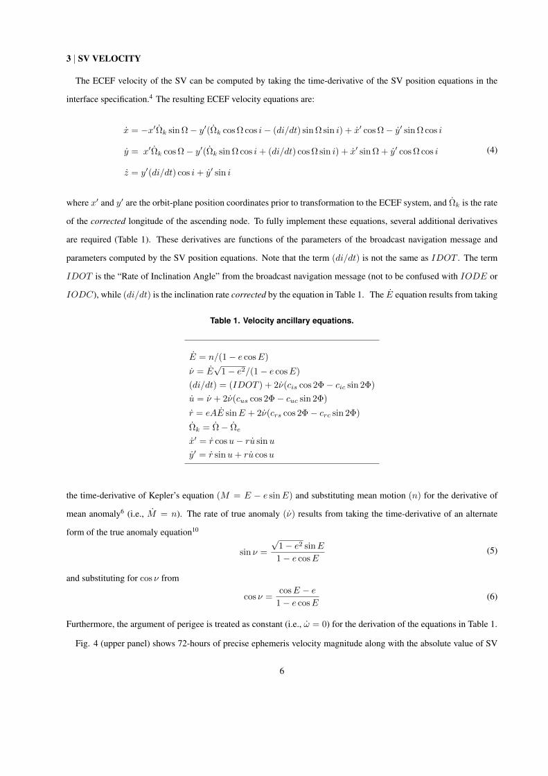
3 | SV VELOCITY

The ECEF velocity of the SV can be computed by taking the time-derivative of the SV position equations in the

interface specification.4 The resulting ECEF velocity equations are:

x = −x′Ωk sin Ω− y′(Ωk cos Ω cos i− (di/dt) sin Ω sin i) + x′ cos Ω− y′ sin Ω cos i

y = x′Ωk cos Ω− y′(Ωk sin Ω cos i+ (di/dt) cos Ω sin i) + x′ sin Ω + y′ cos Ω cos i

z = y′(di/dt) cos i+ y′ sin i

(4)

where x′ and y′ are the orbit-plane position coordinates prior to transformation to the ECEF system, and Ωk is the rate

of the corrected longitude of the ascending node. To fully implement these equations, several additional derivatives

are required (Table 1). These derivatives are functions of the parameters of the broadcast navigation message and

parameters computed by the SV position equations. Note that the term (di/dt) is not the same as IDOT . The term

IDOT is the “Rate of Inclination Angle” from the broadcast navigation message (not to be confused with IODE or

IODC), while (di/dt) is the inclination rate corrected by the equation in Table 1. The E equation results from taking

Table 1. Velocity ancillary equations.

E = n/(1− e cosE)

ν = E√

1− e2/(1− e cosE)

(di/dt) = (IDOT ) + 2ν(cis cos 2Φ− cic sin 2Φ)

u = ν + 2ν(cus cos 2Φ− cuc sin 2Φ)

r = eAE sinE + 2ν(crs cos 2Φ− crc sin 2Φ)

Ωk = Ω− Ωe

x′ = r cosu− ru sinu

y′ = r sinu+ ru cosu

the time-derivative of Kepler’s equation (M = E − e sinE) and substituting mean motion (n) for the derivative of

mean anomaly6 (i.e., M = n). The rate of true anomaly (ν) results from taking the time-derivative of an alternate

form of the true anomaly equation10

sin ν =

√1− e2 sinE

1− e cosE(5)

and substituting for cos ν from

cos ν =cosE − e

1− e cosE(6)

Furthermore, the argument of perigee is treated as constant (i.e., ω = 0) for the derivation of the equations in Table 1.

Fig. 4 (upper panel) shows 72-hours of precise ephemeris velocity magnitude along with the absolute value of SV

6

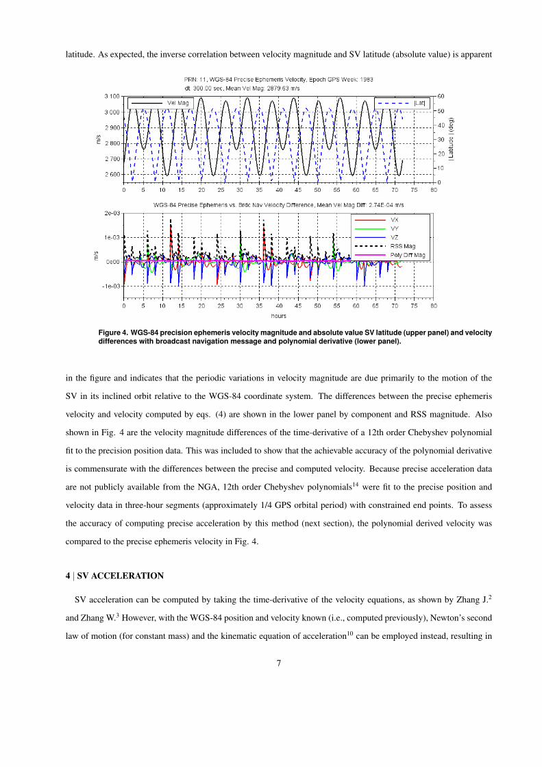
latitude. As expected, the inverse correlation between velocity magnitude and SV latitude (absolute value) is apparent

Figure 4. WGS-84 precision ephemeris velocity magnitude and absolute value SV latitude (upper panel) and velocitydifferences with broadcast navigation message and polynomial derivative (lower panel).

in the figure and indicates that the periodic variations in velocity magnitude are due primarily to the motion of the

SV in its inclined orbit relative to the WGS-84 coordinate system. The differences between the precise ephemeris

velocity and velocity computed by eqs. (4) are shown in the lower panel by component and RSS magnitude. Also

shown in Fig. 4 are the velocity magnitude differences of the time-derivative of a 12th order Chebyshev polynomial

fit to the precision position data. This was included to show that the achievable accuracy of the polynomial derivative

is commensurate with the differences between the precise and computed velocity. Because precise acceleration data

are not publicly available from the NGA, 12th order Chebyshev polynomials14 were fit to the precise position and

velocity data in three-hour segments (approximately 1/4 GPS orbital period) with constrained end points. To assess

the accuracy of computing precise acceleration by this method (next section), the polynomial derived velocity was

compared to the precise ephemeris velocity in Fig. 4.

4 | SV ACCELERATION

SV acceleration can be computed by taking the time-derivative of the velocity equations, as shown by Zhang J.2

and Zhang W.3 However, with the WGS-84 position and velocity known (i.e., computed previously), Newton’s second

law of motion (for constant mass) and the kinematic equation of acceleration10 can be employed instead, resulting in

7

a much simpler formulation.

f = ao + aR + 2(ω × vR) + (ω × rR) + ω × (ω × rR) (7)

All vectors are in the ECEF (WGS-84) coordinate system – the earth-centered inertial (ECI) system is not used. The

vectors in eq. (7) are defined below:

f specific force, i.e. net external force per (constant) mass

ao acceleration of the origin of the rotating frame

aR acceleration with respect to the rotating frame

ω angular velocity of the rotating frame

rR position with respect to the rotating frame

vR velocity with respect to the rotating frame

Note that ao = 0 (null vector) because the origin of WGS-84 is fixed at the center of mass of Earth, co-located with

origin of the inertial frame. Let ω = [0, 0, Ωe]T and ω = 0, where Ωe is the WGS-84 Earth rotation rate. Solve for

aR, the desired acceleration vector with respect to the ECEF frame,

aR = f − 2(ω × vR)− ω × (ω × rR) (8)

Let f be the two-body gravitational force-per-mass expressed in ECEF coordinates. Carrying out the vector cross

products in eq. (8), the equations for ECEF acceleration in component form become

ax = −µxr3

+ 2yΩe + xΩ2e

ay = −µyr3− 2xΩe + yΩ2

e

az = −µzr3

(9)

where r =√x2 + y2 + z2, and µ is the Earth gravitational parameter (µ = GM). These equations are much less

complex than those of the derivative method and produce the same level of accuracy. For comparison and complete-

ness, the derivative method equations of acceleration are included here without derivation.

x′ = −µxr3

y′ = −µyr3

(10)

8

x =− x′Ω2 cos Ωk + x′ cos Ωk − y′ sin Ωk cos ik

+ y′(

(Ω2k + (dik/dt)

2) sin Ωk cos ik + 2Ωk(dik/dt) cos Ωk sin ik

)− 2x′Ωk sin Ωk − 2y′(Ωk cos Ωk cos ik − (dik/dt) sin Ωk sin ik)

(11)

y =− x′Ω2 sin Ωk + x′ sin Ωk + y′ cos Ωk cos ik

− y′(

(Ω2k + (dik/dt)

2) cos Ωk cos ik − 2Ωk(dik/dt) sin Ωk sin ik

)+ 2x′Ωk cos Ωk − 2y′(Ωk sin Ωk cos ik + (dik/dt) cos Ωk sin ik)

(12)

z = −y′(dik/dt)2 sin ik + 2y′(dik/dt) cos ik + y′ sin ik (13)

Note the difference in complexity between eqs. (9) and (10) - (13). Also note that eq. (10) is the two-body gravitational

acceleration in the orbit-plane coordinate system of the broadcast navigation position equations (see Table 3), where

x′ points to the ascending node of the SV orbit, and y′ points to 90 in-track in the orbital plane. (There is no z′

position component because the SV position vector lies entirely in the orbital plane, z′ = 0 always). The final three

broadcast navigation position equations are, in fact, the orbit-plane SV position coordinates transformed to ECEF by an

orthogonal transformation comprising orbital inclination (ik) and longitude of the ascending node (Ωk). Incorporating

non-spherical Earth gravity effects in eq. (10) would first require transforming the gravitational acceleration from

ECEF to orbit-plane coordinates. This would also introduce a non-zero z′ acceleration component. Including non-

spherical gravity in the derivative eqs. (10) - (13) is possible, but unnecessarily complex. It is much simpler to modify

the kinematic eqs. (9) to include non-spherical gravity, as shown below in eq. (14). Earth oblateness (J2) is the

dominant perturbing force acting on the SV orbits. The third-body gravity of the Sun and Moon are approximately

one order of magnitude less than J2, and solar radiation pressure is approximately two orders of magnitude less.6, 8

The broadcast navigation orbit model includes correction terms to account for J2 and other perturbations, nominally

over the span of four hours. It follows that computing acceleration with the dominant J2 effects is commensurate with

the accuracy of the broadcast navigation position and velocity.

An example 72-hour acceleration comparison is shown in Fig. 5. The upper panel shows acceleration magnitude

and SV latitude (absolute value), revealing strong correlation due to the motion of the SV in the WGS-84 coordinate

frame. The lower panel shows the RSS magnitude differences compared to precise values (i.e., time-derivative of the

Chebyshev velocity polynomials) for the derivative method and the kinematic method. Also shown in the lower panel

is the effect of including oblate Earth gravity (J2) in the kinematic method, which improves the mean acceleration

magnitude difference by approximately one order of magnitude. The numerical value for J2 was derived from the

fully-normalized coefficient C20 of the EGM-2008 gravity model15 (by convention: J2 = −√

5C20). The kinematic

9

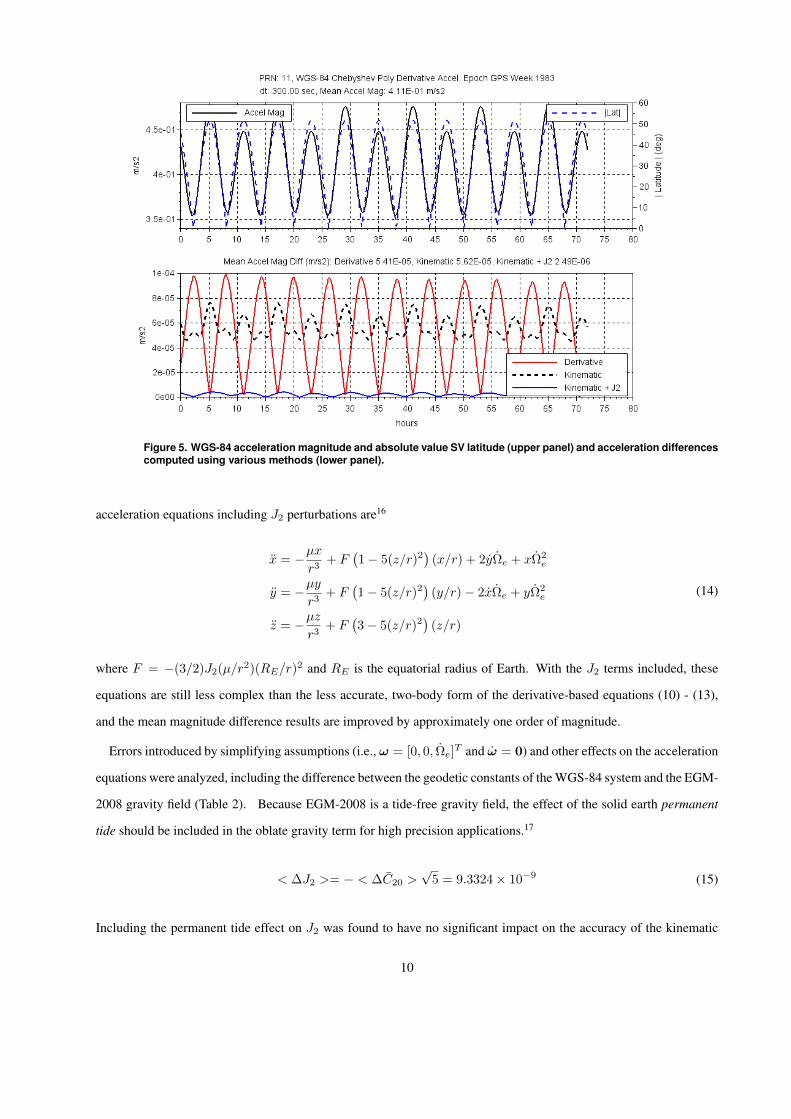
Figure 5. WGS-84 acceleration magnitude and absolute value SV latitude (upper panel) and acceleration differencescomputed using various methods (lower panel).

acceleration equations including J2 perturbations are16

x = −µxr3

+ F(1− 5(z/r)2

)(x/r) + 2yΩe + xΩ2

e

y = −µyr3

+ F(1− 5(z/r)2

)(y/r)− 2xΩe + yΩ2

e

z = −µzr3

+ F(3− 5(z/r)2

)(z/r)

(14)

where F = −(3/2)J2(µ/r2)(RE/r)2 and RE is the equatorial radius of Earth. With the J2 terms included, these

equations are still less complex than the less accurate, two-body form of the derivative-based equations (10) - (13),

and the mean magnitude difference results are improved by approximately one order of magnitude.

Errors introduced by simplifying assumptions (i.e., ω = [0, 0, Ωe]T and ω = 0) and other effects on the acceleration

equations were analyzed, including the difference between the geodetic constants of the WGS-84 system and the EGM-

2008 gravity field (Table 2). Because EGM-2008 is a tide-free gravity field, the effect of the solid earth permanent

tide should be included in the oblate gravity term for high precision applications.17

< ∆J2 >= − < ∆C20 >√

5 = 9.3324× 10−9 (15)

Including the permanent tide effect on J2 was found to have no significant impact on the accuracy of the kinematic

10

Table 2. Geodetic parameters. The WGS-84 value for µ comes from the broadcast navigation equations in theIS, not the separately published value.

Parameter WGS-84 EGM-2008µ (m3/s2) 3.986005× 1014 3.986004415× 1014

RE (meters) 6378137.0 6378136.3C2,0 −0.484165143790815× 10−3

C2,1 −0.206615509074176× 10−9

S2,1 +0.138441389137979× 10−8

acceleration equations (see Fig. 6). The final value of J2 used for evaluation was J2 = 0.0010826262.

Figure 6. WGS-84 acceleration differences with various corrections applied for comparison.

Also considered were the effects of polar motion – the location of the true Earth rotation axis with respect to the

conventional pole. Because the J2 oblate gravity term is dominant over the higher order terms, the approximate mean

pole location, or Earth Orientation Parameters (EOP), can be derived from the gravity field coefficients,17

xp ≈C2,1√3C2,0

6.48× 105

π= 0.051 arcsec

yp ≈−S2,1√3C2,0

6.48× 105

π= 0.341 arcsec

(16)

which include the conversion from radians to arc-seconds. Polar motion EOP data from the International Earth Ro-

tation and Reference Systems Service (IERS)18 from 1962 to 2018 are plotted in Fig. 7, the mean values from eqs.

11

(16) indicated by dashed lines. From the figure, the “worst case” maximum polar motion EOP for this ≈ 60 year data

set is seen to be approximately xp = 0.05 arcsec and yp = 0.6 arcsec. The mean and maximum polar motion had no

significant effect on the computed SV acceleration (Fig. 6). The effects of omitting higher order gravity perturbations

(up to spherical harmonic degree and order twenty – 20x20) were also found to be insignificant at the precision level

of the kinematic acceleration equations, as shown by Fig. 6. Using the precise ephemeris values for position and

velocity in lieu of the less accurate computed values in the kinematic acceleration equations was also found to have

insignificant impact. Finally, Earth precession (≈ 50 arcsec per year) and polar motion rate were analyzed and found

to have no significant effect on SV acceleration. This analysis shows that the accuracy of the kinematic equations

for SV acceleration is not significantly affected by the simplifying assumptions and omission of perturbations when

deriving the equations.

Figure 7. Polar motion Earth Orientation Parameters (EOP), 1962 - 2018. Mean values indicated by dashed lines.

5 | SV CLOCK RELATIVISTIC CORRECTION

The SV clock error (or offset) relative to GPS Time at time t is modeled as

∆tSV = af0 + af1(t− toc) + af2(t− toc)2 + ∆tr (17)

where toc is the clock data reference time, and af0, af1, and af2 are polynomial coefficients unique to each SV clock

and sent in the broadcast navigation message. The last term, ∆tr, is the unique relativistic correction arising from the

12

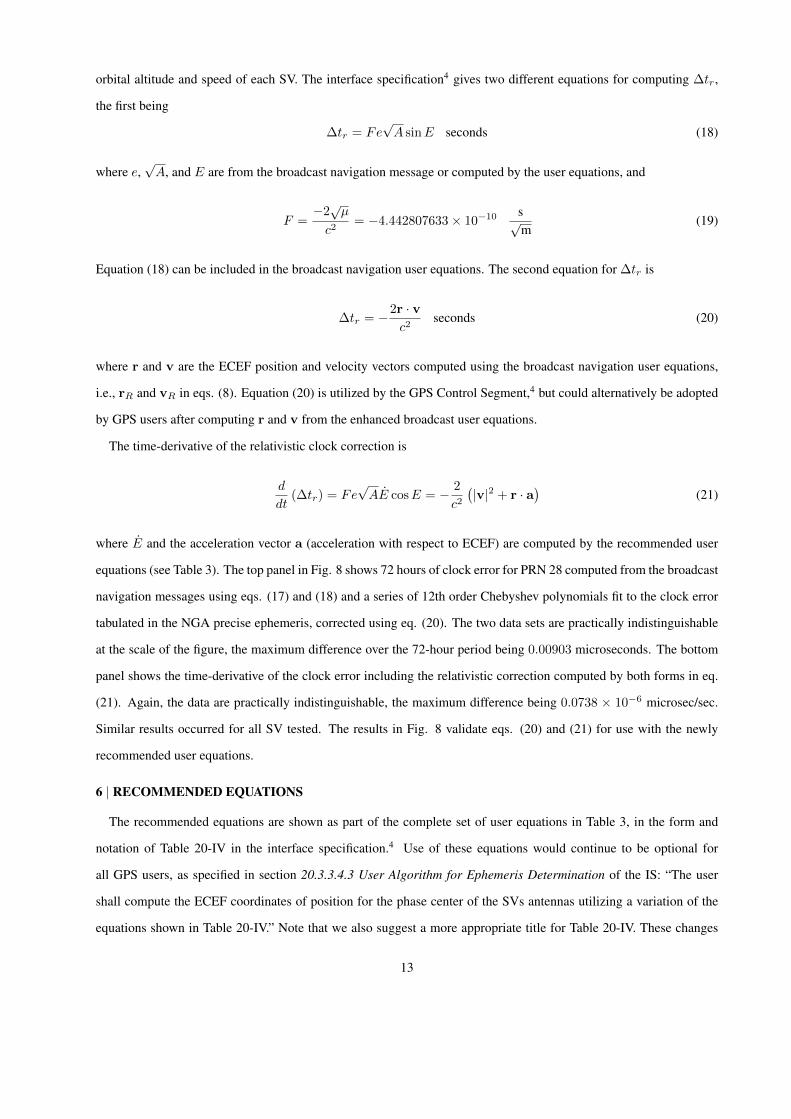
orbital altitude and speed of each SV. The interface specification4 gives two different equations for computing ∆tr,

the first being

∆tr = Fe√A sinE seconds (18)

where e,√A, and E are from the broadcast navigation message or computed by the user equations, and

F =−2√µ

c2= −4.442807633× 10−10

s√m

(19)

Equation (18) can be included in the broadcast navigation user equations. The second equation for ∆tr is

∆tr = −2r · vc2

seconds (20)

where r and v are the ECEF position and velocity vectors computed using the broadcast navigation user equations,

i.e., rR and vR in eqs. (8). Equation (20) is utilized by the GPS Control Segment,4 but could alternatively be adopted

by GPS users after computing r and v from the enhanced broadcast user equations.

The time-derivative of the relativistic clock correction is

d

dt(∆tr) = Fe

√AE cosE = − 2

c2(|v|2 + r · a

)(21)

where E and the acceleration vector a (acceleration with respect to ECEF) are computed by the recommended user

equations (see Table 3). The top panel in Fig. 8 shows 72 hours of clock error for PRN 28 computed from the broadcast

navigation messages using eqs. (17) and (18) and a series of 12th order Chebyshev polynomials fit to the clock error

tabulated in the NGA precise ephemeris, corrected using eq. (20). The two data sets are practically indistinguishable

at the scale of the figure, the maximum difference over the 72-hour period being 0.00903 microseconds. The bottom

panel shows the time-derivative of the clock error including the relativistic correction computed by both forms in eq.

(21). Again, the data are practically indistinguishable, the maximum difference being 0.0738 × 10−6 microsec/sec.

Similar results occurred for all SV tested. The results in Fig. 8 validate eqs. (20) and (21) for use with the newly

recommended user equations.

6 | RECOMMENDED EQUATIONS

The recommended equations are shown as part of the complete set of user equations in Table 3, in the form and

notation of Table 20-IV in the interface specification.4 Use of these equations would continue to be optional for

all GPS users, as specified in section 20.3.3.4.3 User Algorithm for Ephemeris Determination of the IS: “The user

shall compute the ECEF coordinates of position for the phase center of the SVs antennas utilizing a variation of the

equations shown in Table 20-IV.” Note that we also suggest a more appropriate title for Table 20-IV. These changes

13

Figure 8. SV clock error: broadcast navigation message vs. precise ephemeris polynomial (top panel), and clockdrift rate (bottom panel).

and improvements are also applicable to Table 30-II in the IS,4 as well as Table 20-II in IS-GPS-705E,19 Table 3.5-2

in IS-GPS-800E,20 and other similar documents.

Table 3: Recommended updated Table 20-IV for Interface Specifica-

tion IS-GPS-200J.

Table 20-IV. Elements of Coordinate Systems

Table 20-IV. Broadcast Navigation User Equations

µ = 3.986005× 1014 meters3/sec2 WGS 84 value of the earth’s gravitational constant for

GPS user

Ωe = 7.2921151467× 10−5 rad/sec WGS 84 value of the earth’s rotation rate

A =(√

A)2

Semi-major axis

n0 =

õ

A3Computed mean motion (rad/sec)

tk = t− t∗oe Time from ephemeris reference epoch

n = n0 + ∆n Corrected mean motion

(table continues)

14

Table 3 (continued)

Mk = M0 + ntk Mean anomaly

Mk = Ek − e sinEk Kepler’s Equation for Eccentric Anomaly (may be

solved by iteration) (radians)

Kepler’s equation (Mk = Ek − e sinEk) solved

for eccentric anomaly (Ek) by iteration:

E0 = Mk - Initial value (radians)

Ej = Ej−1 +Mk − Ej−1 + e sinEj−1

1− e cosEj−1- Refined value, three iterations, (j = 1, 2, 3)

Ek = E3 - Final value

νk = tan−1

sin νkcos νk

True Anomaly

= tan−1√

1−e2 sinEk/(1−e cosEk)(cosEk−e)/(1−e cosEk)

νk = 2 tan−1

(√1 + e

1− etan

Ek2

)True anomaly (unambiguous quadrant)

Ek = cos−1e+cos νk1+e cos νk

Eccentric Anomaly

Φk = νk + ω Argument of Latitude

δuk = cus sin 2Φk + cuc cos 2Φk Argument of Latitude Correction

δrk = crs sin 2Φk + crc cos 2Φk Radius Correction

δik = cis sin 2Φk + cic cos 2Φk Inclination Correction

uk = Φk + δuk Corrected Argument of Latitude

rk = A(1− e cosEk) + δrk Corrected Radius

ik = i0 + δik + (IDOT)tk Corrected Inclination

x′k = rk cosuk Positions in Orbital Plane

y′k = rk sinuk

Ωk = Ω0 + (Ω− Ωe)tk − Ωetoe Corrected longitude of ascending node

xk = x′k cos Ωk − y′k cos ik sin Ωk Earth-fixed coordinates

yk = x′k sin Ωk + y′k cos ik cos Ωk

zk = y′k sin ik

* t is GPS system time at time of transmission, i.e., GPS time corrected for transit time (range/speed of light).

Furthermore, tk shall be the actual total time difference between the time t and the epoch time toe, and must

account for beginning or end of week crossovers. That is, if tk is greater than 302,400 seconds, subtract

604,800 seconds from tk. If tk is less than -302,400 seconds, add 604,800 seconds to tk.

(table continues)

15

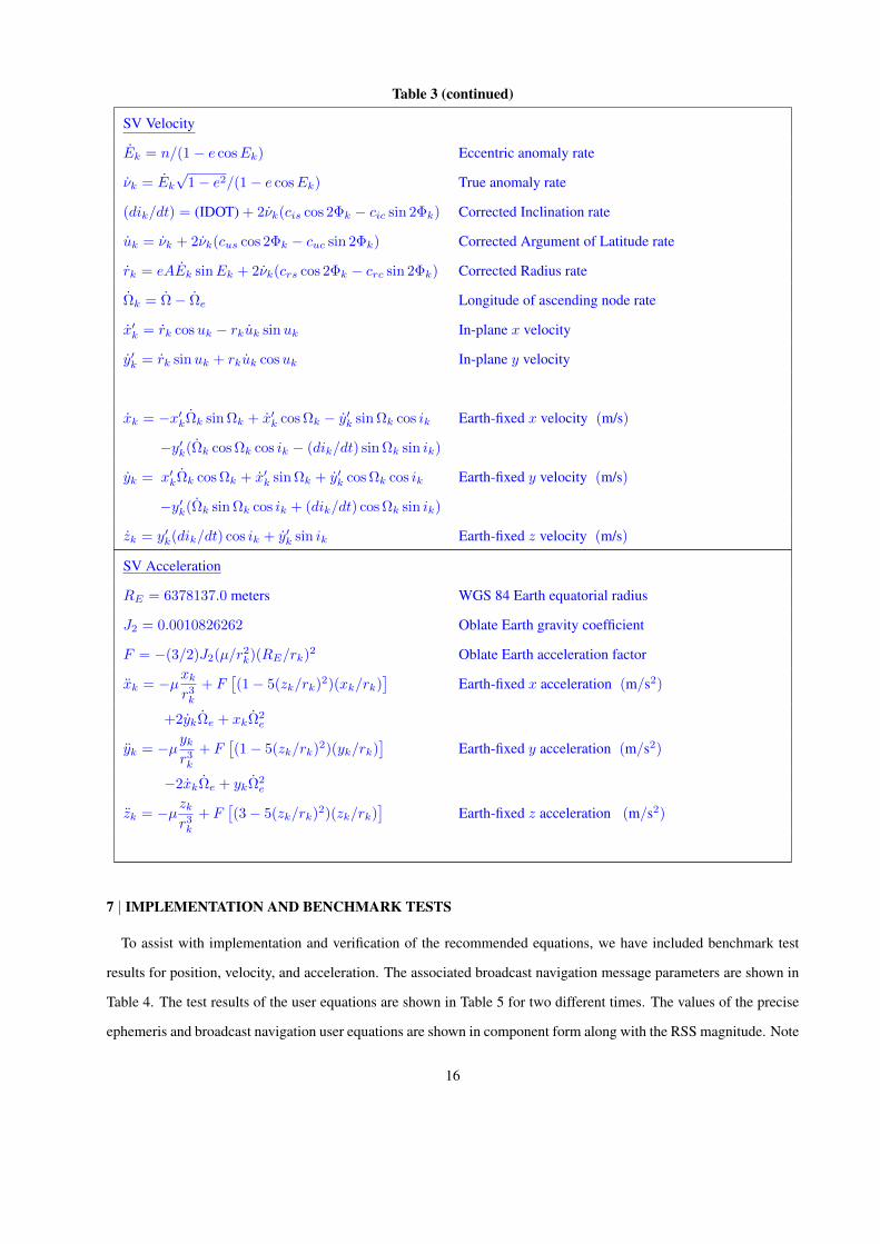
Table 3 (continued)

SV Velocity

Ek = n/(1− e cosEk) Eccentric anomaly rate

νk = Ek√

1− e2/(1− e cosEk) True anomaly rate

(dik/dt) = (IDOT) + 2νk(cis cos 2Φk − cic sin 2Φk) Corrected Inclination rate

uk = νk + 2νk(cus cos 2Φk − cuc sin 2Φk) Corrected Argument of Latitude rate

rk = eAEk sinEk + 2νk(crs cos 2Φk − crc sin 2Φk) Corrected Radius rate

Ωk = Ω− Ωe Longitude of ascending node rate

x′k = rk cosuk − rkuk sinuk In-plane x velocity

y′k = rk sinuk + rkuk cosuk In-plane y velocity

xk = −x′kΩk sin Ωk + x′k cos Ωk − y′k sin Ωk cos ik Earth-fixed x velocity (m/s)

−y′k(Ωk cos Ωk cos ik − (dik/dt) sin Ωk sin ik)

yk = x′kΩk cos Ωk + x′k sin Ωk + y′k cos Ωk cos ik Earth-fixed y velocity (m/s)

−y′k(Ωk sin Ωk cos ik + (dik/dt) cos Ωk sin ik)

zk = y′k(dik/dt) cos ik + y′k sin ik Earth-fixed z velocity (m/s)

SV Acceleration

RE = 6378137.0 meters WGS 84 Earth equatorial radius

J2 = 0.0010826262 Oblate Earth gravity coefficient

F = −(3/2)J2(µ/r2k)(RE/rk)2 Oblate Earth acceleration factor

xk = −µxkr3k

+ F[(1− 5(zk/rk)2)(xk/rk)

]Earth-fixed x acceleration (m/s2)

+2ykΩe + xkΩ2e

yk = −µykr3k

+ F[(1− 5(zk/rk)2)(yk/rk)

]Earth-fixed y acceleration (m/s2)

−2xkΩe + ykΩ2e

zk = −µzkr3k

+ F[(3− 5(zk/rk)2)(zk/rk)

]Earth-fixed z acceleration (m/s2)

7 | IMPLEMENTATION AND BENCHMARK TESTS

To assist with implementation and verification of the recommended equations, we have included benchmark test

results for position, velocity, and acceleration. The associated broadcast navigation message parameters are shown in

Table 4. The test results of the user equations are shown in Table 5 for two different times. The values of the precise

ephemeris and broadcast navigation user equations are shown in component form along with the RSS magnitude. Note

16

that for acceleration the precise values were computed from the derivatives of Chebyshev polynomials fit to the precise

ephemeris velocity data, as described earlier.

Table 4. Broadcast navigation message parameters used for benchmark tests: GPST 7 Jan 2018, 00:00:00.0

Parameter Value Parameter ValuePRN 11 cic 0.199303030968E − 06crs −0.965625000000E + 01 Ω0 −0.657960408566E + 00∆n 0.583845748090E − 08 cis 0.173225998878E − 06M0 −0.286954703389E + 01 i0 0.903782727230E + 00cuc −0.379979610443E − 06 crc 0.293218750000E + 03e 0.167867515702E − 01 Ω 0.173129682312E + 01

cus 0.277347862720E − 05 Ω −0.868929051526E − 08√A 0.515375480270E + 04 IDOT 0.789318592573E − 10toe 0.000000000000E + 00 GPS Week 0.198300000000E + 04

Table 5. Benchmark test results.

GPST 7 Jan 2018 00:35:00.0

Position (m) xk yk zk RSSBroadcast Nav 3166192.017 −21511945.818 −15899623.697 26936715.065Precise Ephemeris 3166191.446 −21511947.161 −15899624.824 26936716.607

Velocity (m/s) xk yk zk RSSBroadcast Nav 1533.973749 −1209.904136 2000.871636 2796.503314Precise Ephemeris 1533.973891 −1209.904144 2000.871617 2796.503382

Acceleration (m/s2) xk yk zk RSSBroadcast Nav −0.224186 0.100579 0.324295 0.406870Precise Ephem. Poly. −0.224188 0.100577 0.324296 0.406871

GPST 7 Jan 2018 01:50:00.0

Position (m) xk yk zk RSSBroadcast Nav 7847635.362 −25169173.996 −4315772.358 26715137.871Precise Ephemeris 7847635.584 −25169175.522 −4315773.249 26715139.518

Velocity (m/s) xk yk zk RSSBroadcast Nav 595.709009 −259.303963 2970.973426 3041.182478Precise Ephemeris 595.708923 −259.304060 2970.973219 3041.182268

Acceleration (m/s2) xk yk zk RSSBroadcast Nav −0.160162 0.305506 0.090248 0.356554Precise Ephem. Poly. −0.160162 0.305506 0.090249 0.356554

17

8 | SUMMARY

Accurate SV position modeling is required for basic GPS navigation (positioning). SV velocity and acceleration

modeling are required for more advanced navigation and other purposes such as receiver velocity determination and

GPS/INS integration. The current interface specification includes equations for computing SV position only. We

present equations for extending the broadcast navigation user equations to compute SV velocity and acceleration.

Previous work in this area has been published, but the methods herein are validated over a longer period of time

using multiple broadcast navigation messages. Additionally, the kinematic form of the acceleration equations are less

complex and improve mean magnitude differences by approximately one order of magnitude when oblate Earth gravity

effects are included. The new methods were validated using three days (6 GPS orbit periods) of precise ephemeris data

from the NGA. For acceleration data, the derivative of a 12th order Chebyshev polynomial fit to the velocity data was

used. Also analyzed were the effects of the permanent tide on the J2 gravity coefficient, mean and maximum polar

motion effects, polar motion rate, precession, and higher order gravity. The recommended equations are provided in

the format and notation of the existing user equations table in the interface specification, and benchmark test results

are provided to ease with implementation and validation.

ACKNOWLEDGMENTS

We thank Air Force Space Command Chief Scientist Dr. Joel Mozer, Deputy Chief Scientist Dr. Michele Gau-

dreault, their staff, and Mr. Anthony Flores of SAIC for their support with this research and development effort.

DISCLAIMER

The views expressed in this paper are those of the authors and do not reflect the official policy or position of the

United States Air Force, Department of Defense, or the U.S. Government.

ORCID

Blair F. Thompson https://orcid.org/0000-0002-7541-6575

Steven W. Lewis https://orcid.org/0000-0002-5070-7691

REFERENCES

1. Remondi B. Computing satellite velocity using the broadcast ephemeris. GPS Solutions. 2004;8:181–183.

2. Zhang J, Zhang K, Grenfell R, Deakin R. GPS Satellite Velocity and Acceleration Determination Using the Broad-

cast Ephemeris. The Journal of Navigation. The Royal Institute of Navigation. 2006;59.

3. Zhang W, Ghogho M, Enrique LE. Extension of the GPS Broadcast Ephemeris to Determine Satellite Velocity and

Acceleration. European Navigation Conference - Global Navigation Satellite Systems (ENC-GNSS), Naples, Italy;

2009.

4. Global Positioning Systems Directorate Systems Engineering and Integration Interface Specification IS-GPS-200J;

25 Apr 2018.

18

5. National Imagery and Mapping Agency. Department of Defense World Geodetic System 1984: Its Definition and

Relationships with Local Geodetic Systems. NIMA Technical Report TR8350.2. 3rd ed.; 3 Jan 2000.

6. Misra P, Enge P. Global Positioning System: Signals, Measurements, and Performance. Lincoln, Mass.: Ganga-

Jamuna Press; 2001.

7. Colwell P. Solving Kepler’s Equation Over Three Centuries. Richmond, Virginia: Willmann-Bell; 1993.

8. VanDierendonck A, Russell S, Kopitzke E, Birnbaum M. The GPS Navigation Message. NAVIGATION. 1978;25(2).

9. Battin R., An Introduction to the Mathematics and Methods of Astrodynamics. New York: American Institute of

Aeronautics and Astronautics; 1987.

10. Vallado D. Fundamentals of Astrodynamics and Applications. 4th ed. Hawthorne, California: Microcosm Press;

2013.

11. Prussing J, Conway B. Orbital Mechanics. 2nd ed., Oxford: Oxford University Press; 2013.

12. Hofmann-Wellenhof B, Lichtenegger H, Collins J. Global Positioning System: Theory and Practice. 4th revised

ed. New York: Springer-Verlag Wien; 1997.

13. National Geospatial-Intelligence Agency (NGA). Global Positioning System precise ephemeris repository.

ftp://ftp.nga.mil/pub2/gps/pedata/

14. Montenbruck O, Gill E. Satellite Orbits: Models, Methods, and Applications. Berlin: Springer; 2001.

15. Pavlis N, Holmes S, Kenyon S, Factor J. The development and evaluation of the Earth Gravitational Model 2008

(EGM2008). Journal of Geophysical Research. 1978;117(B04406).

16. Schaub H, Junkins J. Analytical Mechanics of Space Systems. Reston, Virginia: American Institute of Aeronautics

and Astronautics; 2003.

17. Seidelmann P. ed. Explanatory Supplement to the Astronomical Almanac. Sausalito, California: University Sci-

ence Books; 1992.

18. International Earth Rotation and Reference Systems Service. Earth orientation data repository.

https://www.iers.org/IERS/EN/DataProducts/EarthOrientationData/eop.html

19. Global Positioning Systems Directorate Systems Engineering and Integration Interface Specification IS-GPS-

705E; 25 Apr 2018.

20. Global Positioning Systems Directorate Systems Engineering and Integration Interface Specification IS-GPS-

800E; 25 Apr 2018.

19