computing contour trees in all dimensions

Computational Geometry 24 (2003) 75–94www.elsevier.com/locate/comgeo

Computing contour trees in all dimensions

Hamish Carra, Jack Snoeyinkb,∗, Ulrike Axenc

a Department of Computer Science, University of British Columbia, Vancouver, BC, Canadab Department of Computer Science, University of North Carolina at Chapel Hill, NC, USA

c School of EECS, Washington State Univ., Pullman, WA, USA

Received 26 January 2001; received in revised form 8 August 2001; accepted 15 August 2001

Communicated by P. K. Agarwal and L. Arge

Abstract

We show that contour trees can be computed in all dimensions by a simple algorithm that merges two trees. Ouralgorithm extends, simplifies, and improves work of Tarasov and Vyalyi and of van Kreveld et al. 2002 Elsevier Science B.V. All rights reserved.

Keywords: Iso-surfaces; Simplicial meshes; Morse theory; Resolving singularities

1. Introduction

Many imaging technologies and scientific simulations produce data in the form of sample points withintensity values. One way to visualize this data is to convert it into geometric models by thresholding orby taking level sets. In this paper, we focus on one tool that can help in choosing threshold values or ininteractive exploration of such data: thecontour tree.

Contour trees were used by van Kreveld et al. [28] to compute isolines on terrain maps in geographicinformation systems. With terrain maps, a surface model is computed from elevation values at samplepoints in the plane. Isolines, often called contours, are the curves that can be seen on a topographic map,and consist of points at a given height. Contours can be traced from a surface model relatively easily,given a starting point, or “seed” on each. Van Kreveld et al. use the contour tree to generate “seed sets”for any query height value, guaranteeing that each contour has at least one seed.

We use the contour tree to compute seed sets, to trace whole or partial isosurfaces inR3, and to

determine important values of the height function where topological changes occur in the level sets;

* Corresponding author.E-mail addresses: [email protected] (H. Carr), [email protected] (J. Snoeyink), [email protected] (U. Axen).

0925-7721/02/$ – see front matter 2002 Elsevier Science B.V. All rights reserved.PII: S0925-7721(02)00093-7

76 H. Carr et al. / Computational Geometry 24 (2003) 75–94

these changes may correspond to important phenomena in the data studied. While van Kreveld et al. dodiscuss the extension of their approach toR

3, their algorithm runs in quadratic time, which is prohibitive.Tarasov and Vyalyi [26] gave an O(N logN) algorithm for computing contour trees inR3, whereN is

the number of simplices in the decomposition of the data. We describe their algorithm and the handlingof singularities in more detail later, but their approach can multiply the number of simplices by a factorof 360, and is difficult to implement.

Our algorithm for contour trees begins with Tarasov and Vyalyi’s idea of three passes through the data,but makes the following simplifications and improvements. The first two sweeps do not maintain levelsets, but construct “join” and “split” trees, which store partial topological information about the data.We then apply a simple merge procedure to obtain the contour tree. The resulting algorithm handlesmultiple singularities and extends to all dimensions. Because there are some applications in whichmultiple singularities must be replaced by simple singularities, we also observe that Tarasov and Vyalyi’sapproach to resolving singularities can be extended to all dimensions.

After reviewing isosurfaces in Section 2, we define contour trees and look at their properties inSection 3. We then give our algorithm to construct contour trees in Section 4. Finally, in Section 5, weextend Tarasov and Vyalyi’s resolution of singularities to arbitrary dimensions. We state our conlusionsin Section 6, and give some future directions in Section 7.

2. Isosurfaces

Suppose that we are given a set ofn points {p1,p2, . . . , pn} in a fixed-dimensional spaceRd , withcorresponding scalar measurements{h1, h2, . . . , hn}. We assume that thehi are unique, perhaps byperturbation of our data using simulation of simplicity [10].

To extend the data to the entire space, we choose a meshM with vertex set{p1,p2, . . . , pn}. Meshesused for isosurfaces include regular rectilinear meshes (also known asvoxels or cuberilles) [1,8,9,13,15,16,18,19,29,30], regular simplicial meshes [26,28,29,31], and irregular meshes [14,18]. We then choosea continuous functionf to interpolate at points not in{p1,p2, . . . , pn}, and require thatf (pi)= hi: thisis typically a piecewise-linear function. For convenience, we useheight to refer to the function value.

A level set of f at some height h is the set{x ∈ Rd | f (x) = h}, and may consist of 0,1, or more

connected components. In 2-D, these connected components are calledisolines, and in 3-D,isosurfaces.We usecontour as a general term for a connected component of a level set in a space of arbitrarydimension.

If we think of the heightf (x) as time and watch the evolution of the level sets off over time, thenwe see contours appear, split, change genus, join, and disappear. Thecontour tree, which we define inSection 3, is a graph that tracks contours of the level set as they split and appear or join and disappear.

2.1. Previous work on isosurfaces

Isosurfaces have been widely used for segmentation and rendering, in fields such as medical imaging[1,18,19], fluid dynamics [18], and X-ray crystallography [9,13]. The principal algorithm used to generateisosurfaces is the “Marching Cubes” algorithm [19], which computes the desired level set by findingthe intersection of the level set with each cell of the mesh. This algorithm has several disadvantages:the isosurface generated may have visible cracks, the time required to render an isosurface is O(N) in

H. Carr et al. / Computational Geometry 24 (2003) 75–94 77

the number of cells, and the algorithm fails to distinguish between the contours of the level set. Thefirst disadvantage, that visible cracks appear in the generated model, can be dealt with by Nielsen andHamann’s Asymptotic Decider [21], or by subdividing the cells into simplices (inR

3, tetrahedra). As wesee in Section 3.1, a simplicial mesh is required for the contour tree algorithm, so we choose to subdividethe cells into simplices.

As regards the run-time, various techniques have been proposed to reduce the cost of generating anindividual isosurface to as little as O(logN + k), wherek is an output-sensitive term. These techniquesinclude octrees [30], span space [18], interval trees [7–9], extrema graphs [15,16], segment trees [2,14],and contour trees [3,28]. Of these, octrees, span space, and interval trees require large run-time datastructures(�(N) in the size of the mesh), and retain the inability to distinguish contours of the level set.One reason for this is that these techniques fail to take advantage of the fact that each contour must beconnected: each intersection of a cell and a contour is treated as a separate object.

In contrast, the extrema graph, segment tree, and contour tree approaches take advantage of theconnectivity of individual contours. If we start at a cell known to intersect the isosurface (aseed cell), itis possible to “follow” the contour out the faces of the cell to adjacent cells, and repeat until a completecontour has been traced. The task remaining is then to specify sufficient seed cells to guarantee thatany contour at any isovalue intersects at least one of the seed cells. This can be done interactively [14],heuristically (extrema graphs [15,16]), by a mark-and-sweep algorithm [2], or using contour trees [3,28].

3. Contour trees

The contour tree was introduced by Boyell and Ruston [5], as a summary of the evolution of contourson a map (i.e. in 2-D), and used by Freeman and Morse to find terrain profiles in a contour map [11]. Ithas been used for image processing and geographic information systems [12,17,24,25], but principally in2-D applications. It appears that van Kreveld et al. were the first to identify its applicability to isosurfacesas well as isolines [28]. Since the contour tree is related to the field of Morse theory, we will make someremarks about Morse theory in Section 3.1, then give a definition of the contour tree in Section 3.2,a definition of a related structure called the augmented contour tree in Section 3.3, and a summary ofprevious work in Section 3.4.

3.1. Morse theory

The field of Morse theory [4,20,23] studies the changes in topology of level sets as the heighth isvaried. Points at which the topology of the level sets change are calledcritical points. Morse theoryrequires that the critical points are isolated—i.e., that they occur at distinct points and values. A functionthat satisfies this condition is called aMorse function. All points other than critical points are calledregular points and do not affect the number or genus of the contours.

In order to take advantage of this, we choose our meshM to be a simplicial mesh, and our functionfto be a piecewise-linear function such that:

(1) f is a linear function within each simplex, and(2) f (pi)= hi for all i = 1, . . . , n.


(a) (b) (c)

(d) (e) (f)

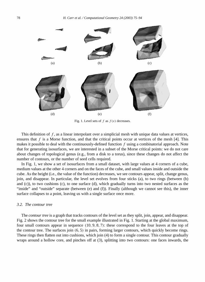
Fig. 1. Level sets off asf (x) decreases.

This definition off , as a linear interpolant over a simplicial mesh with unique data values at vertices,ensures thatf is a Morse function, and that the critical points occur at vertices of the mesh [4]. Thismakes it possible to deal with the continuously-defined functionf using a combinatorial approach. Notethat for generating isosurfaces, we are interested in a subset of the Morse critical points: we do not careabout changes of topological genus (e.g., from a disk to a torus), since these changes do not affect thenumber of contours, or the number of seed cells required.

In Fig. 1, we show a set of isosurfaces from a small dataset, with large values at 4 corners of a cube,medium values at the other 4 corners and on the faces of the cube, and small values inside and outside thecube. As the height (i.e., the value of the function) decreases, we see contours appear, split, change genus,join, and disappear. In particular, the level set evolves from four sticks (a), to two rings (between (b)and (c)), to two cushions (c), to one surface (d), which gradually turns into two nested surfaces as the“inside” and “outside” separate (between (e) and (f)). Finally (although we cannot see this), the innersurface collapses to a point, leaving us with a single surface once more.

3.2. The contour tree

Thecontour tree is a graph that tracks contours of the level set as they split, join, appear, and disappear.Fig. 2 shows the contour tree for the small example illustrated in Fig. 1. Starting at the global maximum,four small contours appear in sequence(10,9,8,7): these correspond to the four leaves at the top ofthe contour tree. The surfaces join(6,5) in pairs, forming larger contours, which quickly become rings.These rings then flatten out into cushions, which join (4) to form a single contour. This contour graduallywraps around a hollow core, and pinches off at (3), splitting into two contours: one faces inwards, the


Fig. 2. Contour tree for Fig. 1.

other outwards. The inward contour contracts until it disappears at (2): the outward contour expands untilit reaches the global minimum (1).

In the foregoing description, we refer to the evolution of level sets as we vary the height. We makethis “evolution” more precise by defining an equivalence relation between two contours. We define ajointo be a critical pointx with an ε-neighbourhood that intersects at least 2 contours atf (x) + δ, whereδ, ε are suitably small values. Asplit is then a critical pointx with an ε-neighbourhood that intersectsat least 2 contours atf (x)− δ. Note that alocal maximum x must have anε-neighbourhood that doesnot intersect any contours atf (x) + δ. Similarly, a local minimum x must have anε-neighbourhoodthat does not intersect any contours atf (x)− δ. Collectively, we refer to joins, splits, local maxima andlocal minima ascritical points: these critical points are a subset of the critical points in Morse theorySection 3.1. We then define the equivalence relation as follows:

Definition 3.1. Let γ andγ ′ be contours at heightsh andh′, respectively, withh < h′. Thenγ andγ ′ areequivalent(γ ≡ γ ′) if all of the following are true:

(1) neitherγ norγ ′ passes through a join, split, local maximum or local minimum,(2) γ andγ ′ are in the same connected componentΓ of {x: f (x) � h}, and there is no joinxi ∈ Γ such

thath < hi < h′, and(3) γ andγ ′ are in the same connected component∆ of {x: f (x) � h′}, and there is no splitxi ∈∆ such

thath < hi < h′.

We refer to the equivalence classes of this relation ascontour classes. Contours that do not passthrough critical points belong to contour classes that map 1–1 with open intervals(hi, hj), wherexi andxj are critical points andxi < xj . We describe a contour class as beingcreated at j , athj , or atxj , andbeingdestroyed at i, athi, or atxi , thus preserving the intuitive description of a sweep from high to lowvalues. Contours that do pass through critical points must be the sole members of the contour classes


to which they belong (i.e., finite contour classes). This correspondence between critical points and finitecontour classes, and between open intervals and infinite contour classes, leads to the definition of thecontour tree for a simplicial mesh:

We define thecontour tree, illustrated in Fig. 2, as a graph(V ,E). Following van Kreveld et al. [28]we refer toV andE assupernodes andsuperarcs, respectively.

The setV contains a supernode for each finite contour class (i.e., for each critical point.) Wedistinguish two types of supernodes: Aninterior supernode corresponds to a critical point at whichat least one infinite contour class is created, and at least one infinite contour class is destroyed. Aleafsupernode corresponds to a local maximum, at which an infinite contour class is created, or a localminimum, at which an infinite contour class is destroyed.

The setE contains a superarc for each infinite contour class. Specifically, if and only if an infinitecontour class is created at the critical point corresponding to the supernodeu and destroyed at the criticalpoint corresponding tov, then the superarc(u, v) ∈E.

3.3. The augmented contour tree

For some purposes, such as the generation of isosurfaces, information about vertices that are notcritical points is also required. We augment the contour tree with the remaining points to produce anaugmented contour tree. For each vertexxi in the mesh, take the contourγi to which xi belongs, andinsertxi into the superarc representing the contour class[γi]. Again following van Kreveld et al., we referto the resulting vertices and edges of the graph asarcs andnodes. Note that this replaces the superarcsbetween supernodes with a path consisting of arcs and nodes.

Because of difficulties illustrating the behaviour of level sets in 3-D, we have constructed a small 2-Dmesh (Fig. 3), with the same contour tree (Fig. 2) as our original 3-D mesh (Fig. 1). We will continueusing this mesh as an example for the balance of this paper: since the algorithm works in arbitrarydimensions, nothing is lost by this choice. Note that, in this 2-D example, the vertices with non-integerlabels are not critical points: Fig. 4(a) shows the augmented contour tree for this mesh. Clearly, if weknow the nodes and arcs, we can generate the supernodes and superarcs. We simplify the presentation of

Fig. 3. A small 2-D example, with the same contour tree as Fig. 1.


(a) (b) (c)

Fig. 4. A small 2-D example, continued. (a) Augmented contour tree. (b) Join tree. (c) Split tree.

the algorithm by working only with the nodes and arcs, and use “contour tree” to refer to the augmentedcontour tree for the balance of this paper (see Fig. 4(a) for an example).

3.4. Previous work

Van Kreveld et al. [28] reported the first efficient algorithm for constructing contour trees. Thisalgorithm performs the extraction in O(N logN) time in 2-D data fields, and O(N2) time in higherdimensions, whereN is the number of simplices (triangles) in the mesh of then data points. Thealgorithm performs a sweep from low to high value, maintaining each contour, and examines the data setlocally to determine when saddle points are encountered and how to deal with them. Multi-saddle pointsare treated as a set of ordinary saddle points. The most time-consuming step is merging contours. In theplane, the running time is reduced to O(N logN) by always merging a smaller contour into a larger; acoordinated search in both contours is used to determine which is the smaller.

Tarasov and Vyalyi [26] presented an O(N logN) algorithm for 3-D data fields. Their algorithmperforms three sweeps: one sweep to identify joins, a second to identify splits, and a third to combinethe results of the two sweeps. Again, the level set is maintained at all times during the sweep. Multi-saddle points are dealt with by a complicated preprocessing step (see Section 5). Running time is keptto O(N logN) by a variation of the method used by van Kreveld et al. in the plane. Finally, boundaryeffects at the edge of the dataset are handled by special cases inside the algorithm.

In both algorithms, two factors contribute to the runtime: the initial sort takes O(n logn) time, andmaintaining the level sets takes O(N logN) time. Bounds on the number of simplices,N , areN =�(n)

and N = O(n d/2�), for a mesh withn vertices ind dimensions. In dimensions greater than 2, thedifference betweenN andn can become significant for irregular meshes. It is, however, always possibleto construct a mesh in any fixed dimension such thatN =�(n) (for example, a regular grid). As a result,the difference betweenn andN is, in most instances, a small constant factor.


4. The contour tree algorithm

We propose an improved algorithm for constructing the contour tree for a real-valued fieldF

interpolated over a simplicial mesh ofn vertices andN simplices, with the following characteristics:

(1) time requirements of O(n logn+Nα(N)) for constructing augmented contour trees, in any numberof dimensions,

(2) space requirements of O(N) for the mesh and O(n) additional working storage,(3) simple treatment of boundary effects, and(4) simple treatment of multi-saddle points.

The algorithm has two stages: in the first stage, we build ajoin tree and asplit tree to identify contourjoins and splits (Section 4.1). In the second stage, we merge these two trees to obtain the contour tree(Section 4.2).

Although the algorithm applies to any arbitrary dimension, the illustrations are in two dimensions forclarity (see Fig. 3 for our example).

4.1. Join and split trees

In this subsection, we introduce thejoin tree andsplit tree for a height graphG (a graph with associatedheights). We demonstrate that the join treeJM of the simplicial meshM used to define our height fieldFis identical to the join treeJC of the contour treeC of F . We then present an algorithm for constructingJC(= JM) in O(n logn+Nα(N)) time and O(n) space.

The join tree is a graph that encapsulates all joins in the contour tree; the correspondingsplit treeencapsulates all splits. These trees are dual if we negate all heights, so we will examine only the join treein detail.

We define aheight graph to be any graphG with heights{hi} associated with the vertices{xi}. Forexample, the meshM underlying our functionf is a height graph. Throughout the rest of Section 4,we use the notationG+i to refer to the subgraph ofG induced by the vertices with height> hi. Also,although the join tree is notionally on the same set of vertices asG, we adopt the convention that ifxi isa vertex inG, thenyi is the corresponding vertex in the join tree.

Definition 4.1. The join treeJG of a height graphG is the graph on the verticesy1, . . . , y‖G‖ in whichtwo verticesyi andyj , with hi < hj , are connected when:

(1) xj is the smallest-valued vertex of some connected componentΓ of G+i , and(2) xi is adjacent inG to a vertex ofΓ .

In Fig. 4(b) and (c), we give the join and split trees corresponding to the 2-D example mesh in Fig. 3.In order for the join tree to be useful, we must relate it to the height field that we are studying: we do so

by showing thatJC = JM , i.e., that the contour treeC and the meshM have the same join tree. We needa couple of preliminary lemmas to show that the connected components ofC+i andM+i are identical.


Fig. 5. Constructing a graph path from a path in space.

Lemma 4.2. xi and xj belong to the same component of M+k precisely when they belong to the samecomponent of {x: f (x) > hk}.

Proof. Suppose thatxi andxj belong to the same component ofM+k for any k. Therefore, there mustbe a path inM connectingxi and xj such that each vertex on the path has height> hk. But sinceM is embedded in the volume over whichf is defined, this path also connectsxi and xj in the set{x: f (x) > hk}, so xi andxj belong to the same component of{x: f (x) > hk}. Now suppose thatxiandxj belong to the same component ofM+k . Thenxi andxj are connected in{x: f (x) > hk} by somepathP . If we trace the pathP through the simplices of the meshM (as in Fig. 5), we can “push”P upto edges of the simplex that are above the valuehk (see Fig. 5). This gives us a pathP ′ connectingxi andxj in the meshM . It follows thatxi andxj belong to the same component ofM+k exactly when they (xiandxj ) belong to the same component of{x: f (x) > hk}. ✷Lemma 4.3. For each component in C+k , there exists a component in M+k containing exactly the samevertices (and vice versa).

Proof. Proof is by finite induction, starting with the highest vertexxn, for which the property is triviallytrue. For convenience, assume that the vertices are indexed in sorted order: i.e., thath1 < h2 < · · ·< hn.

Assuming that the hypothesis is true fork � i � n, consider the vertexxk−1: the only differencebetween the components ofM+k andM+k−1 is that the arcs fromxk to adjacent, higher vertices have beenadded to the latter. We break the proof into three cases, based on the type of vertex thatxk is: localmaximum, join, or neither:

If xk is a local maximum, then it has no arcs leading upwards, and there are no edges added toM+k toobtainM+k−1. A local maximum only has one edge, to a lower vertex. Thus no edges are added toC+k toobtainC+k−1, and the hypothesis follows.

If xk is a join, then letxkxj be any edge incident toxk in C+k−1. From Section 3.3,xk andxj botheither belong to some superarc, or are endpoints of it. Since the superarcs and supernodes correspondto contour classes, we take the union of these contour classes, and obtain a connected set in the originalspace of points with values betweenhk andhj . Therefore, there is a pathP from xk to xj in this set.


But this set is contained in some componentγ of {x: f (x) > hk−1}. So, by Lemma 4.2,xk andxj mustalso be connected inM+k−1. This is true for each edgexkxj in C (with hk < hj). Also, the components ofM+k and{x: f (x) > hk} have the same vertex sets by the induction hypothesis. Thus, it follows thatxk isconnected to the same components ofM+k in M as inC.

As a result, the component ofM+k−1 to whichxk belongs will correspond directly to the component of{x: f (x) > hk−1} to whichxk belongs. Components to whichxk does not connect will be unaffected, sowe conclude that the components ofM+k−1 andC+k−1 contain the same vertices, as required.

If xk is neither a local maximum nor a join, then it must be adjacent to exactly one component ofM+kand an argument similar to that of Case II applies to show that the components ofM+k−1 andC+k−1 containthe same vertices.✷Theorem 4.4. The contour tree C and the mesh M have the same join tree (i.e., JC = JM).

Proof. In Definition 4.1, I defined the join tree of a height graphG in terms of the components ofG+i .By Lemma 4.3, these components are identical inC andM , and we saw in the proof of Lemma 4.3 thatxi will be connected to the same components ofC+i andM+i . It follows immediately from Definition 4.1thatJC = JM . ✷

Having now defined the join tree, we now present an algorithm to compute it efficiently.

Algorithm 4.1 (Algorithm To Construct JM ). Given the meshM , we compute the join treeJM of themesh (see Fig. 6) as follows. Since Definition 4.1 requires that we know the components ofM+i todetermine edges incident toxi , we use Tarjan’s union-find algorithm [27] to determine connectivity.This information is stored in array calledComponent. In addition, Definition 4.1 requires that we knowthe smallest-valued vertex in each component, so we maintain a separate array,LowestVertex, for thisinformation.

We sort the vertices of the mesh by the corresponding height values, then process the vertices fromhighest to lowest value. For each vertexxi , we add each edgexixj to a union-find structure iffhi < hj .After each vertexxi has been processed, all edges between two vertices whose values are at leasthi mustbe contained in the union-find structure. At each vertexxi , we generate one edge in the join tree for each

Algorithm to compute JC = JM :Input: the mesh M, with vertices x1 . . . xn in sorted order (i.e., h1 < h2 . . .hn)

Output: the join tree JC, with vertices y1 . . . yn

1. for i := n downto 1 do:

(a) Component[i] := i(b) LowestVertex[i] :=yi(c) for each vertex xj adjacent to xi

i. if (j < i) or (Component[i] = Component[j]) skip xjii. UFMerge(Component [i], Component[j])iii. AddEdgeToJoinTree(yi, LowestVertex[Component[j]])iv. LowestVertex[Component[j]] :=yi

Fig. 6. Algorithm 4.1 to construct a join tree.


component ofM+i to whichxi connects, and update both the union-find structure and the smallest vertexof each component. After we have processed all vertices, the join tree has been computed.

To see that we construct the join tree with this procedure, suppose that we are processing vertexxi ,and thatxixk is an edge fromxi to a vertexxk whose heighthk is higher thanhi . Because Tarjan’s union-find algorithm computes connectivity incrementally,Component represents the connectivity of all edgesadded so far. Since each edge inM+i has both ends higher thanxi , they must already have been added, andComponent therefore represents the connectivity ofM+i at this stage. Now, sincehi < hk, xk has alreadybeen processed, and must belong to some componentΓ of M+i . Since this satisfies the second conditionof Definition 4.1, we useLowestVertex to identify the smallest-valued vertexxj of Γ , and add edgexixjto the output if it has not already been added. After processingxi , we setLowestVertex[Component[i]]to point toxi , as it is now the lowest-valued vertex in the component to which it belongs.

This algorithm requires a sort in O(n logn) time, followed by the union-find algorithm inO(N +Mα(M)), whereN is the number of edges in the mesh, andM is the number of union-findmerges performed (at most equal to the number of local maxima in the mesh). Note thatM +m � t �2(M +m)− 1, wheret is the number of supernodes in the contour tree, andM,m are the number oflocal maxima and minima, respectively. Thus, we can express the bound for constructing the join andsplit trees as O(n logn+N + tα(t)).

4.2. Merging to form the contour tree

In this section, we give the main contribution of this paper: a simple algorithm to merge join andsplit trees. First we give an overview of the concept behind the merge algorithm, define some terms, andprovide a recursive proof that the merge algorithm works. We then give a non-recursive implementationof the algorithm that takes O(n) time.

To reconstruct the contour treeC from the join treeJC and split treeSC , we identify a leafxi of C andits incident edgexixj . We deletexi from C, JC andSC to produce a reduced graphC \ xi , along with thecorresponding join treeJC\xi andSC\xi . We repeat the process until all edges ofC have been identified.

Before embarking on the reconstruction, we define some terms that we rely on. We useup-arc anddown-arc to refer to arcs leading up and down from a given vertex in a given graph, andup-degree(δ+)anddown-degree(δ−) to refer to the number of up- and down- arcs at a given vertex. Note that the up-degree of a vertexyi in JC is identical to the up-degree of the corresponding vertexxi in C, and thatthe down-degree of a vertexyi in JC is always 1, except at the global minimum vertex, where it is 0.Similarly, a vertexzi in the split tree has identical down-degree to the corresponding vertexxi in C, andthe up-degree of a vertexzi in the split tree is 1 except at the global maximum. Since we can find theup-degree ofxi (in C) by examiningyi (in JC) and the down-degree ofxi (in C) by examiningzi in SC ,we note that we can tell the exact degree of any vertexxi in C, even if we do not know the edges inC.In particular, we can use this information to identify which vertices are leaves ofC. For convenience, wewill refer to leaves ofC with up-degree of 0 asupper leaves and those with down-degree of 0 aslowerleaves.

When deleting a vertexxi from C, we preserve connectivity by contracting the incident arcs into asingle arc (see Fig. 7). This operation is calledreduction to distinguish it from the simple removal of avertex from a graph. Theorem 4.8 will then show that applying the reduction operation on the join andsplit trees gives the join and split trees of the new, smaller graph.


Fig. 7. Vertex reductions applied to vertices 2 and 7.

Definition 4.5. DefineC � xi , the reduction of a graphC by a vertexxi whose up-degree and down-degree are both� 1, to be:

(1) If xi has arcsxixj up andxixk down inC, then:C � xi = C \ xi ∪ xjxk .(2) Otherwise,C � xi = C \ xi .

Lemma 4.6. If xi is an upper leaf in C, and yiyj is the incident arc to yi in JC , then xixj is the incidentarc to xi in C.

Proof. Let xi belong to some componentγ in C+j . Suppose thatxi is not the only vertex inγ . Then,sinceγ is a connected component, there is some other vertexxk in γ to which xi is connected. ByDefinition 4.1,xi is the smallest-valued vertex inγ , soxixk must be an up-arc atxi . But, sincexi is anupper leaf, it has no up-arcs. It follows thatxi is the only vertex inγ . Applying Definition 4.1,yiyj is anarc ofJC , thenxj must be connected to some vertex inγ . But, sincexi is the only vertex inγ , it followsthatxj is connected toxi . ✷

We now consider what happens when we remove an edgexixj from C. Recall that our convention(from Definition 4.1) is thatxi refers to a vertex inC, andyi the same vertex inJC .

Lemma 4.7. If xi is a leaf of C, and yjyk is an arc of the corresponding join tree JC such that hj < hk,and i �= j, k, then yjyk is also an arc of JC\xi .

Proof. By Definition 4.1,xj is adjacent to some vertexxl in the componentγ of C+j to whichxk belongs:i.e., there exists some pathP from xl to xk in γ . Sincexi is a leaf, it could only be at an end of the path, butxj , xk are the path-ends, andxi �= xj , xk . Thus,P exists inC \xi , and therefore inC \x+ij , the subgraph ofC \ xi consisting of edges whose vertices have higher values thanxi does. Sincexjxl is also inC \ xi, xjis adjacent to the componentρ of C \ x+ij to whichxk belongs.

Note that each pathP connecting two vertices ofγ is also inρ, except for paths starting or endingat xi : thus the vertices ofγ are the same as those ofρ, with the possible exception ofxi . It then followsthatxk is the smallest-valued vertex ofρ, so by Definition 4.1,yj is adjacent toyk in JC\xi . ✷


Fig. 8. Reducing a join tree at a lower leaf.

Theorem 4.8. If xi is a leaf of a contour tree C, then JC\xi = JC � yi .

Proof. From Lemma 4.7, each edge ofJC that is not incident toyi is also inJC\xi . We know that bothJC andJC\xi are trees, withn− 1 andn− 2 edges, respectively.

Suppose thatyi is a leaf inJC . Then there aren − 2 edges ofJC that are not incident toyi , and byLemma 4.7, each of them must be inJC\xi , soJC\xi = JC � yi .

Sinceyi is not a leaf inJC , δ+(yi)= 1; sinceyi is not the global minimum,δ−(yi)= 1. After excludingthese two edges, onlyn− 3 edges ofJC remain that are not incident toyi . Again, by Lemma 4.7, eachof them must be inJC\xi , so only one edge remains to be found.

Let the down-arc atyi beyiyj , and the up-arc beyiyk (see Fig. 8). From Definition 4.1,xi belongs tosome componentγ of C+j , andxj is adjacent to some vertexxl in γ . Note thatxlxj must be a down-arc,and sincexi has no down-arcs,xl cannot bexi . Also, sincexi is the smallest-valued vertex inγ , hi < hl.

Consider the componentρ of C+i to which xk belongs. Since each vertex ofρ has value� hk , andhk > hj , we know thatρ ⊆ γ andxk must be inγ . Sincexi is the smallest-valued vertex ofγ , the onlyarc ofγ that is not inρ must be the arc incident toxi , soρ = γ \ xi . But this must be a component of(C \ xi)+i , the subgraph ofC \ xi containing only vertices with heights> hi . Sincexl �= xi , it followsthatxl must have been connected toxi in γ , as wasxk . Thenxl must be connected toxk by a path whosevertices all have values> hi . Therefore,xl andxk belong to the same component ofρ, and sincexk isthe smallest-valued vertex ofδ \ xi, yj must be connected toyk in JC\xi .

Note thatyjyk cannot be an arc inJC , becauseyiyj yk would then be a cycle inJC . Thus, we haveadded an arc to then−3 arcs that we had already shown to be inJC� yi , for a total ofn−2. SinceJC\xiis a tree onn−1 vertices, there are no more arcs to be found inJC\xi . From Definition 4.5, it follows thatJC\xi = JC � yi . ✷

We can implement this algorithm to run in time that is linear in the size of the tree. In fact, byeliminating the tail-recursion and using static data structures forC, JC , andSC , this step changes frombeing the slowest of the three sweeps in Tarasov and Vyalyi [26] to being the fastest.

Algorithm 4.2 (Algorithm To Merge JC and SC). In the merge algorithm (Fig. 9), we assume that thejoin treeJC and split treeSC are stored as adjacency lists using half-arcs: that is, each arcyiyj in JC isstored as a directed arcα in yi ’s adjacency list, linked to a directed arcα′ in yj ’s adjacency list.


Algorithm to compute the contour tree:Input: the join tree JC and split tree SC corresponding to C,stored as adjacency lists

Output: the contour tree C

1. For each vertex xi, if up-degree in JC+ down-degree in SCis 1, enqueue xi

2. Initialize C to an empty graph on ‖JC‖ vertices3. While leaf queue size > 1

(a) Dequeue the first vertex, xi, on the leaf queue.(b) If xi is an upper leaf, find incident arc yiyj in JC.

Else find incident arc zizj in SC.(c) Add xixj to C.(d) JC← JC � yi, SC← SC � zi.(e) If xj is now a leaf, enqueue xj.

Fig. 9. Algorithm 4.2 to merge the join and split trees.

Note that, since there aren− 1 edges in the contour tree, the main loop of the algorithm iteratesn− 1times, leaving one vertex on the queue at the end. The first and last 4 steps of this algorithm on theexample in Fig. 4 are shown in Fig. 10.

As we observed in Section 3.3, this algorithm in fact computes the augmented contour tree, but we canconvert this to the contour tree proper in O(n) time by applying the reduction operation to each regularvertex: these can readily be identified in the contour tree, since they are the only vertices to have onearc leading upwards and one downwards. Alternately, it is not difficult to modify Algorithm 4.1 so thatinstead of storing the lowest vertex, we store the vertex at which the last join or maximum occurred.Edges are only added to the join tree when another join is encountered, or at the global minimum. Aftera separate pass to determine the split tree, all supernodes will be present in at least one of the two trees.All supernodes that are only present in the join tree are added to the split tree, along the appropriatearc. Although this reduces the cost of merging to O(t) from O(n), the asymptotic running time of thealgorithm is not improved.

4.3. Boundary effects and multiple singularities

Although we previously reported [6] that special treatment was required for vertices on the boundaryof the data set, it turns out that the algorithm given above needs no special cases for boundary vertices.In addition, no special cases are required for dealing with multiple saddle points, although we extendTarasov and Vyalyi’s result [26] to arbitrary dimensions in Section 5, below.

4.4. Computing the (non-augmented) contour tree

As noted in Section 3.3, the presentation of the algorithm is simpler if we work with the augmentedcontour tree instead of the contour tree, then reduce all regular points in the augmented contour tree toobtain the contour tree. In practice, a slightly more efficient implementation is possible. To compute thecontour tree with Algorithm 4.2, we need to compute the join and split trees for the contour tree, rather


Fig. 10. First four and last four steps of merge algorithm.


(a) (b) (c) (d)

Fig. 11. Computing the (non-augmented) contour tree. (a) Join tree. (b) Full join tree. (c) Split tree. (d) Full split tree.

than for the augmented contour tree. This can be done by omitting regular points during the constructionof the join and split trees in Algorithm 4.1. Instead of adding an edge to the join tree at every vertex, wedo so only at joins and at the global minimum: the upper end of the edge will be the vertex at which thecomponent in the union-find data structure was last changed (i.e., created or merged). This will give us ajoin tree with local maxima, joins and the global minimum only. We augment this join tree with the splitsand local minima, as shown in Fig. 11, then apply Algorithm 4.2 to compute the contour tree.

5. Resolving multiple singularities

The algorithm described by Tarasov and Vyalyi [26] requiressimple singularities, so they describe amethod for breaking multi-saddle points into multiple simple singularities in time O(N lgN). Althoughour algorithm handles multi-saddles, their method is of independent interest for computation of Morsesingularities in higher dimensions; if non-simple singularities are resolved, then a general function on acomplexK is a Morse function. We therefore briefly show that their method applies in all dimensions.We assume familiarity with concepts of PL topology such as barycentric subdivisions, star, and link [22].

We first summarize the subdivision and perturbation given in [26] and extend it trivially to generaldimensions. We then considerably simplify the proof that this method resolves non-simple singularities,and we extend it to all dimensions. Assume thatK is am-dimensional simplicial complex,m � 3, inR

d andf is a general function onK (i.e., f (v) �= f (w) for any pair of verticesv,w ∈ K). The firststep is to construct the barycentric subdivision, sdK , and extendf linearly over sdK . This yields anew functionf0 with the property that no two critical points are adjacent, but which may not be a generalfunction. A small perturbation described in [26] transformsf0 into a general functionf1 overK1= sdK .

Now the star of each non-simple singularity is further refined. Letv be a non-simple saddle point. Foreachk-dimensional simplex in the link ofv, Lk(v), a new so-calledk-vertex is added in the star ofv,St(v), as follows. For each vertexw in Lk(v), a corresponding 0-vertex is added on the edgevw, at apoint which is 1

4 distance fromv to w. For eachk-simplexσ in Lk(v), k � 1, a k-vertex is added inthe (k + 1)-simplex formed byv andσ , at 1

3 distance fromv to the barycenter ofσ . See Fig. 12 for anillustration in 2 dimensions.


Fig. 12. The subdivision of a 2-simplexvwx at a non-simple singularityv.

Simplices of this subdivision are defined as follows. Letσ be am-simplex in St(v), i.e., a simplexof highest dimension; it containsm 0-vertices. These together withv form a newm-simplex. The restof σ is then a prism with two(m− 1)-simplices as bases. Now each cell containing a 1-vertex is startriangulated from the 1-vertex, then each 2-vertex defines a star triangulation to form tetrahedra, and soon up to the(m− 1)-vertex, where the star triangulation results inm-simplices.

The neighborhoods of all non-simple singularities are refined in this manner, yielding a newcomplexK2. Now f1 is extended overK2 to yield a new functionf2. By definition, f1 = f2 at allvertices common toK1 andK2. We now describe the extension off1 to f2, again very similar to thatdescribed in [26].

Let h be a linear function overRd that has different values at all vertices ofK2, and letH be themaximum difference between any two values ofh onK2, i.e.,

H =maxv,w

{h(v)− h(w)

}.

Let δ be the minimum gap between successive values off1 onK1. For each vertexu added in the star ofa non-simple singularityv, let

f2(u)= f1(v)+ δ

2H

(h(u)− h(v)

).

Functionf2 onK2 now has the property that all singularities are simple, i.e., that the level set atf2(v)

divides St(v) into at most three components. Indeed, it is easy to see that all former regular points andsimple singularities are still regular or simple (see [26]), so we restrict ourselves here to proving that aformer non-simple singularityv is regular, and that all points added inK2 are either regular or simple.To see thatv is a regular point, notice that after the local refinement aroundv, St(v) consists only of thesimplices formed by 0-vertices andv. f2 is by construction linear over St(v) and sov must be a regularpoint. Now we use an inductive proof to show that the addedk-vertices are either regular or simple. Wedefine therestricted star or restricted link to be the restriction of the star or link of an added pointu tosimplices formed only by vertices added inK2.

Lemma 5.1. All k-vertices, k � 0, added in the subdivision around non-simple singularities are eitherregular points or simple singularities of f2.

Proof. Let u be a 0-vertex,u is adjacent to two original vertices fromK1: the non-simple singularityv,and the vertexw which was used to constructu. Otherwise,u is only adjacent to other added vertices.


Sincef2 is linear over the simplices formed byv and the added vertices, the level set atf2(u) divides therestricted St(u) into at most two connected components, one with values greater thanf2(u) and the otherwith values less thanf2(u). w either belongs to one of those connected components or it forms its ownconnected component. Thus,u is either a regular point or a simple singularity.

Now let u be ak-vertex,k � 1. By construction,u is not adjacent to any vertices ofK1 other thanthe vertices of thek-simplex that defineu. Again, the restricted St(u) and Lk(u) can be broken bythe level set atf2(u) into at most 2 components. We now make the inductive assumption that a(k − 1)-simplexσ ∈ Lk(u) fromK1 divides Lk(u) further into at most three components and show that under thisassumption, ak-simplex fromK1 in Lk(u) cannot divide Lk(u) further into more than three connectedcomponents. Letσ ∈ Lk(u) be a(k − 1)-simplex fromK1, and letw ∈ Lk(u) be the additional vertexfrom K1 that forms ak-simplex in Lk(u). There are three cases to consider.

(1) Suppose first that some vertices ofσ have value inf2 greater thanf2(u) and others have value lessthanf2(u). Thenw necessarily belongs to one of the existing connected components.

(2) Supposeσ belongs to one of the connected components of the restricted Lk(u). Then Lk(u) withoutw consists of at most two components, andw can increase this to at most three components.

(3) Finally, assume thatσ forms a separate connected component.w is adjacent to bothσ and vertices ofthe restricted Lk(u), so regardless of the value atf2(w), vertexw belongs to an existing component.

These three cases complete the proof.✷Note that in the proof we do not need to distinguish between boundary simplices and interior simplices.

6. Conclusions

Tarasov and Vyalyi [26] stated an algorithm for constructing contour trees in three dimensions, basedon the work of van Kreveld et al. [28]. We have taken this algorithm, simplified it, and extended it toarbitrary dimensions. We have discarded the explicit construction of contours during the third sweep intheir algorithm. In addition, our algorithm needs no special cases or preprocessing to deal with boundaryvertices or with multiple singularities. Our algorithm applies to any arbitrary dimensional data with thesame asymptotic performance, since it is no longer dependent on explicit construction of level sets duringthe sweep. For cases where it is desirable to substitute simple singularities for multiple singularities,we have also extended Tarasov and Vyalyi’s pre-processing step to arbitrary dimensions. We have alsoimproved the asymptotic time bound from O(N logN) to O(n logn+ tα(t)).

7. Future work

We have implemented the algorithm stated for relatively small data sets(< 106 vertices). UnlikeMarching Cubes [19] and its derivatives, we require the input data to be on a simplicial mesh. We intendto modify the algorithm and the contour tree approach to work directly with voxels, and also intend toimplement a parallel algorithm for working with large data sets.


Acknowledgements

Portions of this work were performed while the first two authors were affiliated with the Universityof British Columbia, Vancouver, Canada. Support from Canada’s NSERC through a postgraduatefellowship, a research grant, and the IRIS NCE is gratefully acknowledged. Further support came fromthe University of North Carolina at Chapel Hill.

References

[1] E. Artzy, G. Frieder, G.T. Herman, The theory, design, implementation and evaluation of a three-dimensional surfacedetection algorithm, Computer Graphics and Image Processing 15 (1981) 1–24.

[2] C.L. Bajaj, V. Pascucci, D.R. Schikore, Fast isocontouring for improved interactivity, in: IEEE Proceedings on VolumeVisualization 96, IEEE, 1996, pp. 39–47.

[3] C.L. Bajaj, V. Pascucci, D.R. Schikore, Seed sets and search structures for optimal isocontour extraction, Technical Report99-35, Austin, TX, 1999.

[4] T.F. Banchoff, Critical points and curvature for embedded polyhedra, J. Differential Geom. 1 (1967) 245–256.[5] R.L. Boyell, H. Ruston, Hybrid techniques for real-time radar simulation, in: IEEE Proceedings Fall Joint Computer

Conference 63, IEEE, 1963, pp. 445–458.[6] H. Carr, J. Snoeyink, U. Axen, Computing contour trees in all dimensions, in: Proceedings of the 11th Annual ACM-SIAM

Symposium on Discrete Algorithms, ACM, 2000, pp. 918–926.[7] Y.-J. Chiang, C.T. Silva, I/O optimal isosurface extraction, in: IEEE Proceedings on Visualization 96, IEEE, 1997, pp. 303–

310.[8] Y.-J. Chiang, C.T. Silva, W.J. Schroeder, Interactive out-of-core isosurface extraction, in: IEEE Proceedings an

Visualization 98, IEEE, 1998, pp. 167–174.[9] P. Cignoni, C. Montani, E. Puppo, R. Scopigno, Multiresolution representation and visualization of volume data, IEEE

Trans. on Visualization and Computer Graphics 3 (4) (1997) 352–369.[10] H. Edelsbrunner, E. Mücke, Simulation of simplicity: A technique to cope with degenerate cases in geometric algorithms,

ACM Trans. on Graphics 9 (1) (1990) 66–104.[11] H. Freeman, S. Morse, On searching a contour map for a given terrain elevation profile, J. Franklin Institute 284 (1) (1967)

1–25.[12] C. Gold, S. Cormack, Spatially ordered networks and topographic reconstruction, in: Proceedings of the 2nd International

Symposium on Spatial Data Handling, ACM, 1986, pp. 74–85.[13] B. Guo, Interval set: A volume rendering technique generalizing isosurface extraction, in: IEEE Proceedings on

Visualization 95, IEEE, 1995, pp. 3–10.[14] C. Howie, E.H. Blake, The mesh propagation algorithm for isosurface construction, Computer Graphics Forum 13 (1994)

65–74.[15] T. Itoh, K. Koyamada, Automatic isosurface propagation using an extrema graph and sorted boundary cell lists, IEEE

Trans. on Visualization and Computer Graphics 1 (4) (1995) 319–327.[16] T. Itoh, K. Koyamada, Isosurface extraction by using extrema graphs, IEEE Trans. on Visualization and Computer

Graphics 1 (1995) 77–83.[17] I.S. Kweon, T. Kanade, Extracting topographic terrain features from elevation maps, CVGIP: Image Understanding 59

(1994) 171–182.[18] Y. Livnat, H.-W. Shen, C.R. Johnson, A near optimal isosurface extraction algorithm using the span space, IEEE Trans. on

Visualization and Computer Graphics 2 (1) (1996) 73–84.[19] W.E. Lorenson, H.E. Cline, Marching cubes: A high resolution 3D surface construction algorithm, Computer Graph-

ics 21 (4) (1987) 163–169.[20] J.W. Milnor, Morse Theory, Princeton University Press, Princeton, NJ, 1963.[21] G.M. Nielson, B. Hamann, The asymptotic decider: Resolving the ambiguity in marching cubes, in: IEEE Proceedings on

Visualization 91, IEEE, 1991, pp. 83–91.


[22] C. Rourke, B. Sanderson, Introduction to Piecewise-Linear Topology, Springer, Berlin, 1972.[23] Y. Shinagawa, T.L. Kunii, Y.L. Kergosien, Surface coding based on Morse theory, IEEE Computer Graphics Appl. 11

(1991) 66–78.[24] J.K. Sircar, J.A. Cebrian, Application of image processing techniques to the automated labelling of raster digitized contour

maps, in: Proceedings of the 2nd International Symposium on Spatial Data Handling, ACM, 1986, pp. 171–184.[25] S. Takahashi, T. Ikeda, Y. Shinagawa, T.L. Kunii, M. Ueda, Algorithms for extracting correct critical points and

constructing topological graphs from discrete geographical elevation data, Computer Graphics Forum 14 (3) (1995) C-181–C-192.

[26] S.P. Tarasov, M.N. Vyalyi, Construction of contour trees in 3D in O(n logn) steps, in: Proceedings of the 14th ACMSymposium on Computational Geometry, ACM, 1998, pp. 68–75.

[27] R. Tarjan, Efficiency of a good but not linear set union algorithm, J. ACM 22 (1975) 215–225.[28] M. van Kreveld, R. van Oostrum, C.L. Bajaj, V. Pascucci, D.R. Schikore, Contour trees and small seed sets for isosurface

traversal, in: Proceedings of the 13th ACM Symposium on Computational Geometry, ACM, 1997, pp. 212–220.[29] J. Wilhelms, A. van Gelder, Topological considerations in isosurface generation, Computer Graphics 24 (5) (1990) 79–86.[30] J. Wilhelms, A. van Gelder, Octrees for faster isosurface generation, ACM Trans. on Graphics 11 (3) (1992) 201–227.[31] Y. Zhou, B. Chen, A. Kaufman, Multiresolution tetrahedral framework for visualizing regular volume data, in: IEEE

Proceedings on Visualization 97, IEEE, 1997, pp. 135–142.

computing contour trees in all dimensions

Documents