Contents lists available at ScienceDirect

Computers & Geosciences

journal homepage: www.elsevier.com/locate/cageo

Research paper

Development of a coupled wave-flow-vegetation interaction model

Alexis Beudin, Tarandeep S. Kalra, Neil K. Ganju⁎, John C. Warner

US Geological Survey, Woods Hole, MA 02543, USA

A R T I C L E I N F O

Keywords:Flexible aquatic vegetationCoastal hydrodynamicsNumerical modeling

A B S T R A C T

Emergent and submerged vegetation can significantly affect coastal hydrodynamics. However, most determi-nistic numerical models do not take into account their influence on currents, waves, and turbulence. In thispaper, we describe the implementation of a wave-flow-vegetation module into a Coupled-Ocean-Atmosphere-Wave-Sediment Transport (COAWST) modeling system that includes a flow model (ROMS) and a wave model(SWAN), and illustrate various interacting processes using an idealized shallow basin application. The flowmodel has been modified to include plant posture-dependent three-dimensional drag, in-canopy wave-inducedstreaming, and production of turbulent kinetic energy and enstrophy to parameterize vertical mixing. Thecoupling framework has been updated to exchange vegetation-related variables between the flow model and thewave model to account for wave energy dissipation due to vegetation. This study i) demonstrates the validity ofthe plant posture-dependent drag parameterization against field measurements, ii) shows that the model iscapable of reproducing the mean and turbulent flow field in the presence of vegetation as compared to variouslaboratory experiments, iii) provides insight into the flow-vegetation interaction through an analysis of theterms in the momentum balance, iv) describes the influence of a submerged vegetation patch on tidal currentsand waves separately and combined, and v) proposes future directions for research and development.

1. Introduction

Aquatic vegetation (e.g., mangroves, salt marshes, and seagrasses)plays an important role in estuarine ecosystems by acting as a seabedstabilizer, nutrient sink, and nursery for juvenile fishes and inverte-brates (Hemminga and Duarte, 2000). They are often referred to aseco-engineers because they modify their physical environment to createmore favorable habitat for themselves and other organisms (Joneset al., 1994). For example, seagrasses can reduce sediment resuspen-sion thereby increasing light penetration and potential growth (Carret al., 2010). Evaluating the resilience of estuarine ecosystems requiresgreater insight into the interactions between vegetation, currents,waves, and sediment transport. The relevance of aquatic vegetationin coastal protection from extreme events has become a recurringquestion along with the viability assessment of ecosystem-basedmanagement approaches (Barbier et al., 2008; Temmerman et al.,2013).

Previous laboratory and numerical investigations have focused onthe blade-to-meadow scale (detailed review by Nepf, 2012). Paired withtheoretical analysis, they stand as valuable tools to study vegetated flowdynamics (Fig. 1). However, they do not consider the inherentcomplexity of realistic environments (e.g., spatial variations of vegeta-tion distribution and bathymetry, nonlinear wave-current interac-

tions). Coastal ocean numerical models can be used to investigatethese complex processes, but their resolution often requires parame-terizations to account for small (sub-grid) scale turbulent features ofthe flows, which are particularly important in the presence of vegeta-tion.

The simplest method to account for the influence of vegetation in adepth-averaged flow model is an increase of the bottom roughnesscoefficient (Ree, 1949; Morin et al., 2000). More recently, vegetationhas been parameterized as a source of form drag as opposed to skinfriction relevant to sediment transport in the depth-averaged sense(Chen et al., 2007; Le Bouteiller and Venditti, 2014). However, two-dimensional depth-averaged (2DH) approximations cannot account forthe complex vertical structure of the flow within and over submergedvegetation (Sheng et al., 2012), especially shear layers at the top of thecanopy that enhance vertical mixing (Lapetina and Sheng, 2014;Marjoribanks et al., 2014). To date, few estuary-scale models accountfor the three-dimensional influence of vegetation on the mean andturbulent flow (Temmerman et al., 2005; Kombiadou et al., 2014;Lapetina and Sheng, 2015), and none are part of an open-source,community model. In addition to exerting drag on the mean flow,aquatic vegetation also attenuates waves. While the bed-roughnessapproach has been rather successfully applied to simulate wave heightdecay over vegetation (Möller et al., 1999; de Vriend, 2006; Chen et al.,

http://dx.doi.org/10.1016/j.cageo.2016.12.010Received 16 May 2016; Received in revised form 18 August 2016; Accepted 14 December 2016

⁎ Corresponding author.E-mail address: nganju@usgs.gov (N.K. Ganju).

Computers & Geosciences 100 (2017) 76–86

Available online 15 December 20160098-3004/ Published by Elsevier Ltd.This is an open access article under the CC BY-NC-ND license (http://creativecommons.org/licenses/BY-NC-ND/4.0/).

MARK

2007), the cylinder approach of Dalrymple et al. (1984) provides amore physically based description of wave dissipation by vegetationand its implementation in spectral wave models has been validatedagainst flume experiments (Mendez and Losada, 2004; Suzuki et al.,2012; Wu, 2014; Bacchi et al., 2014).

The present study aims at providing an open-source process-basedmodeling framework that allows comprehensive studies of the inter-actions between hydrodynamics and vegetation, and describing/illus-trating the influence of a submerged vegetation patch on currents andwaves in an idealized shallow basin. We first detail the implementationof flow-vegetation interaction processes within the models, and thenassess the model results using prior studies. We detail the interactionbetween flow and vegetation for a number of idealized cases, thendiscuss future avenues of model application and improvement.

2. Methods

The wave-flow-vegetation module described in this paper is im-plemented as part of the open-source Coupled Ocean-Atmosphere-Wave-Sediment Transport (COAWST) numerical modeling system(Warner et al., 2010), operating on the flow (ROMS) and wave(SWAN) models (Fig. 2) coupled via the Model Coupling Toolkit(MCT) generating a single executable program (Warner et al., 2008a,2008b). The vegetation parameterizations are successively described inthe flow and wave models.

2.1. Flow model

ROMS (Regional Ocean Modeling System) is a three-dimensional,

free surface, finite-difference, terrain-following model that solves theReynolds-Averaged Navier-Stokes (RANS) equations using the hydro-static and Boussinesq assumptions (Haidvogel et al., 2008):

⎛⎝⎜

⎞⎠⎟

ut

v u fv ϕx z

u w ν uz

D F∂∂

+⎯→∙∇ − =− ∂∂

− ∂∂

′ ′− ∂∂

+ +u u(1a)

⎛⎝⎜

⎞⎠⎟

vt

v v fu ϕy z

v w ν vz

D F∂∂

+⎯→∙∇ + =− ∂∂

− ∂∂

′ ′− ∂∂

+ +v v(1b)

ϕz

ρgρ

− ∂∂

− =00 (1c)

ux

vy

wz

∂∂

+ ∂∂

+ ∂∂

=0(1d)

where u v w( , , ) are the velocity vector v⎯→ components in the horizontal(the Cartesian coordinates x and y can be replaced by more generalcurvilinear coordinate ξ and η, in which case additional metric termsappear in the equations) and vertical (z is actually scaled to sigma-coordinate) directions respectively, f is the Coriolis parameter, ϕ is thedynamic pressure (normalized by the reference density of seawater ρ0),ρ is the density, ν is the molecular viscosity, D D( , )u v are the horizontaldiffusive terms calculated with the vector Laplacian of the velocity field,and F F( , )u v are the forcing terms that include wave-averaged forces(Kumar et al., 2012) and vegetation drag force and in-canopy wave-induced streaming (described in the next paragraphs).

The (spatially averaged) vegetation drag force can be approximatedusing a quadratic drag law:

F C b n u u v= 12

+d veg u D v v, ,2 2

(2a)

F C b n v u v= 12

+d veg v D v v, ,2 2

(2b)

where ρ is the (total) density of seawater,CD is the plant drag coefficient(constant assuming a high Reynolds number), bv is the width ofindividual plants, nv is the number of plants per unit area, and u v( , )are the horizontal velocity components at each vertical level in thecanopy of height lv (when upright). A limiter is imposed to prevent thevegetation drag force from having a value large enough to reverse thevelocity direction (see also bottom stress limiter due to wetting anddrying in Warner et al., 2013).

To quantify the reduction of drag due to the bending of flexibleplants, Dijkstra (2012) implemented a lookup table of deflected heightand equivalent drag coefficient based on a detailed one-dimensionalvertical model of plant motion called Dynveg (Dijkstra andUittenbogaard, 2010), while Kombiadou et al. (2014) used an empiricalformula based on laboratory data of Ganthy (2011) for the height of thebent canopy. In the present study, the more generally applicable(across vegetation species and hydrodynamic conditions) approach of

Fig. 1. Sketch of three different flow regimes. The dominant source of turbulence is respectively (from left to right) the bed, the top of the canopy (shear layer), and the stem wakes.

Fig. 2. Diagram showing data exchanges between the flow model, the wave model, andthe vegetation module in COAWST.

A. Beudin et al. Computers & Geosciences 100 (2017) 76–86

77

Luhar and Nepf (2011) has been implemented. An effective bladelength (lve) is defined as the length of a rigid vertical blade thatgenerates the same horizontal drag as the flexible blade of total length(lv), accounting for drag reduction both due to the reduced frontal area(deflected height times width) and to the more streamlined shape of thebent blades. Based on a theoretical plant posture model (described indetails in Luhar and Nepf, 2011), the effective blade length expressioncan be reduced to (Eq. (16) in Luhar and Nepf, 2011):

ll

CaCa B

=1 − 1 − 0. 91+ (8+ )

ve

v

−1/3

−3/2 3/2 (3a)

where Ca is the Cauchy number and B is the buoyancy parameterdefined respectively as:

Ca ρC b U lEI

=0. 5 D v v2 3

(3b)

Bρ ρ gb t l

EI=

( − )v v v v3

(3c)

with I the second moment of area ( b t= /12v v3 for a rectangular section),

tv the blade thickness, E the elastic modulus, and ρv the vegetationtissue density. In Luhar and Nepf (2011) the in-canopy velocitymagnitude U is vertically uniform, while in the present model U variesover depth (U u v= +2 2 ). The actual implementation of the model issubject to verification through the bending angle from vertical of thedeflected canopy (Luhar and Nepf, 2011):

⎛⎝⎜

⎞⎠⎟θ l

l=cos ve

v

−11/3

(3d)

The wave-induced streaming (oscillatory contribution to steadywave stress) in the direction of wave propagation within the vegetationcanopy (observed by Luhar et al., 2010; Luhar and Nepf, 2013) isimplemented in the momentum balance as an additional wave-averaged forcing (similar to streaming in the wave boundary layer) as:

FS k

ρ σ=

∼

∼s vegd veg tot

,, ,

0 (4)

where k∼ is the mean wave number, σ∼ is the mean wave frequency, andSd veg tot, , is the total wave energy dissipation due to vegetation termcalculated in the wave model (Eq. (10)) and exchanged with the flowmodel.

The vertical Reynolds stresses (vertical flux of horizontal momen-tum by turbulent velocity fluctuations) are related to the mean flowthrough the use of an eddy viscosity:

u w K uz

′ ′=− ∂∂M (5a)

v w K vz

′ ′=− ∂∂M (5b)

where the overbar represents a time average and the prime represents afluctuation about the mean, and KM is the eddy viscosity that isparameterized as:

K c k l ν= +M μ1/2 (5c)

where k is the turbulent kinetic energy, l is a turbulent length scale (sizeof the largest turbulent eddies), and cμ is a stratification stabilityfunction (for non-stratified or neutral flow c c= ≈0.55μ μ

0 ). The variables kand l are computed with a generic (GLS) two-equation turbulencemodel (Umlauf and Burchard, 2003 in Warner et al., 2005) that canrepresent several classic turbulence model schemes (e.g., k kl− , k ε− ,and k ω− ):

⎛⎝⎜

⎞⎠⎟

kt

v kz

Kσ

kz

P P B ε∂∂

+⎯→∙∇ = ∂∂

∂∂

+ + + −M

ks veg

(6a)

where σk is the turbulent Schmidt number for k , Ps is the production of k

by shear, Pveg is the production of k by vegetation (see Eq. (7)), B is thebuoyancy flux, and ε is the turbulent dissipation expressed as:

ε c k ψ=( )μp n m n n0 3+ / 3/2+ / −1/ (6b)

where p n m( , , ) is a set of parameters to retrieve the classic turbulencemodels (Table 1 in Warner et al., 2005), and ψ c k l= ( )μ

p m n0 is the genericparameter satisfying the second equation of the turbulence model:

⎛⎝⎜

⎞⎠⎟

ψt

v ψz

Kσ

ψz

ψk

c P c B c εF D∂∂

+⎯→∙∇ = ∂∂

∂∂

+ ( + − − )M

ψwall veg1 3 2

(6c)

where σψ is the turbulent Schmidt number for ψ , c1 and c2 arecoefficients selected to be consistent with the von Karman constantand with experimental observations for decaying homogeneous iso-tropic turbulence (Wilcox, 1998 in Warner et al., 2005), c3 is acoefficient depending on stratification stability, Fwall is a wall proximityfunction, and Dveg is an extra dissipation term due to vegetation (seeEq. (8)).

According to Uittenbogaard (2003), the turbulence production dueto vegetation in Eq. (6a) is expressed as:

P F u F v= ( ) + ( )veg d veg u d veg v, ,2

, ,2

(7)

and the source of enstrophy or dissipation due to vegetation in Eq. (6c)is expressed as:

D cPτ

=vegveg

eff2

(8a)

with τeff defined as the minimum between the dissipation time scale offree turbulence and the dissipation time scale of eddies in between theplants:

τ τ τ= min ( )eff free veg, (8b)

where,

τ kε

=free (8c)

and

⎛⎝⎜⎜

⎞⎠⎟⎟τ L

c P=veg

k veg

2

2

1/3

(8d)

with c c=( ) ≃0.09k μ0 4 and L is the typical length scale between the plants

defined as:

⎛⎝⎜

⎞⎠⎟L z c b t n

n( ) = 1 −

lv v v

v

1/2

(8e)

with cl a coefficient of order unity.The stress exerted on the flow by the bed is calculated using a

quadratic drag coefficient and assuming a logarithmic profile in thebottom cell (Warner et al., 2008a, 2008b). The presence of wavesincreases bottom mixing which affects the bottom resistance experi-enced by a current, and can be interpreted as an apparent increase inthe bottom roughness (Madsen, 1994).

2.2. Wave model

SWAN (Simulating Waves Nearshore) is a third-generation spectralwave model based on the action balance equation (Booij et al., 1999):

Nt

c Nx

c Ny

c Nσ

c Nθ

Sσ

∂∂

+ ∂∂

+∂

∂+ ∂

∂+ ∂

∂=x y σ θ tot

(9)

N being the action density defined as the ratio of the wave energydensity (or variance spectrum) distributed over (intrinsic) wavefrequency (σ) and direction of propagation (θ) divided by frequency( E σ θ σ= ( , )/ ), where c is the propagation velocity. The equation is abalance between local rate of change, advection in the horizontal (x and

A. Beudin et al. Computers & Geosciences 100 (2017) 76–86

78

y) directions, shifting of relative frequency due to variation in waterdepth and current (exchanged between the flow and wave models),depth-induced refraction and additional source/sink terms (S )tot ,namely wave-growth due to wind input, energy transfer due to wave-wave interactions, and dissipation due to white-capping, depth-in-duced breaking, and bottom friction (plus vegetation drag described innext paragraph). SWAN can also account for diffraction, partialtransmission, and reflection.

Wave dissipation due to vegetation is computed with the formula-tion of Mendez and Losada (2004) following the work of Dalrympleet al. (1984) on cylinders, which was implemented in SWAN by Suzukiet al. (2012) as:

⎛⎝⎜⎜

⎞⎠⎟⎟S

πg C b n k

σsinh kl sinh kl

kcosh khE E σ θ=− 2 ( )+3 ( )

3 ( )( , )

∼ ∼ ∼∼ ∼∼d veg D v v

v vtot,

23 3

3 (10)

where CD is a bulk drag coefficient (that may be dependent on theKeulegan-Carpenter number K u T b= /C c p v with uc a characteristic velo-

city acting on the plants, and Tp the wave period), k∼ is the mean wavenumber, σ∼ is the mean wave frequency, h is the water depth, Etot is thetotal wave energy, and E is the wave energy at frequency σ anddirection θ. This term was derived neglecting the shearing generated atthe top of the canopy, and the inertial force caused by the fluidaccelerating past the plant stems (Morison et al., 1950). However,Luhar et al. (2010) underline that the inertia-dominated regime (whenthe wave orbital excursion is much smaller than the drag and shearlength scales) is not relevant for field conditions, and that the energeticcontribution of the work done by the shear stress is typically two orderof magnitude smaller than the energy dissipation due to the drag. Inthe present version of SWAN, the vegetation height lv cannot varyspatially, and therefore the effect of plant reconfiguration undercurrent-forcing on wave dissipation is not currently accounted for.

2.3. Test case configuration

The implementation of the wave-flow-vegetation interactions wereevaluated in the COAWST modeling system with an application to anidealized model domain that represents a 10 km by 10 km and 1 mdeep basin. The model is forced by oscillating the water level on thenorthern edge with a tidal amplitude of 0.5 m and a period of 12 h.Waves are also imposed on the northern edge with a height of 0.5 m,directed to the south (zero angle), with a period of 2 s. The southernedge of the model domain is closed (zero gradient condition for thesurface elevation and the tangential velocity components, and normalvelocity components set to zero). The (western and eastern) sides havea zero gradient boundary condition for the flow and an absorbingcondition for the wave energy. A square patch of vegetation (1 km by1 km) is placed in the middle of the domain. The selected vegetationtype is submerged and designed to resemble eelgrass (Zostera marina).The plant stems are 30 cm high, 0.3 cm wide, and (if flexible) thicknessis set to 0.3 mm thick, mass density to 700 kg/m3 and elastic modulusto 1 GPa (Luhar and Nepf, 2011; J. Testa, pers. comm.). The dragcoefficients in the flow model (CD) and in the wave model (CD ) are set to1 (typical value for a cylinder at high Reynolds number). The density isset to 2500 stems/m2 (packing density a=7.5 m−1) which is a densevegetation canopy according to Ghisalberti and Nepf (2004) and Nepf(2012). The bed roughness is z0=0.05 mm which corresponds to amixture of silt and sand (Soulsby, 1997). The turbulence modelselected is the k ε− scheme. The grid is 100 by 100 in the horizontal(100 m resolution) and has 40 vertical sigma-layers (uniformly dis-tributed). The ROMS barotropic and baroclinic time steps are respec-tively 0.05 s and 1 s, while the SWAN time step and the couplinginterval between ROMS and SWAN are 10 min.

Several scenarios were simulated to evaluate the hydrodynamiceffects of vegetation (Table 1): (1) NV: non-vegetative cases or controlexperiments in which the vegetation module is not activated; (2) T: the

flow model alone with (stiff or flexible) vegetation drag and turbulencemixing; (3) W: the wave model alone with wave energy dissipation dueto stiff vegetation; (4) WC: the wave and flow models coupled but nofree surface elevation fields from the flow model to the wave model(option ZETA_CONST); (5) WWL: flow model and wave model coupledbut no current fields from the flow model to the wave model (optionUV_CONST); (6) FW: full coupling of the flow and wave models.

3. Results

3.1. Model verification

Different components of the model have already been validatedagainst multiple sets of laboratory experiments with rigid vegetation:drag force (Eq. (2)) and turbulent vertical mixing (Eqs. (7)-(8)) byUittenbogaard (2003), and wave dissipation (Eq. (10)) by Suzuki et al.(2012). Here, we focus on the current-vegetation interaction para-meterization using an effective blade length (Eq. (3)) to account forplant reconfiguration when predicting the drag force by flexiblevegetation. The deflected canopy height (ld) is located at the point ofinflection in the vertical velocity profiles (Fig. 1) either simulated by thetest case or measured in and above real eelgrass canopies by Lacy andWyllie-Echeverria (2011) at different phases of the tide. The bending ofthe blade simulated and measured in the field (θ l l= cos ( / ))d v

−1 arecompared to the values obtained from Eq. 3d by normalizing thevelocity at the top of the canopy through a Froude number(Fr U gl= / v ) (Fig. 3). The simulated and the observed bending anglescomply with the semi-empirical model, confirming the validity of theeffective blade length expression of Luhar and Nepf (2011) and itsimplementation in COAWST.

A parameterization of wave-induced streaming by vegetation(analogous to viscous boundary streaming) has been implementedbut remains to be verified against laboratory and field measurements(Luhar et al., 2010 and Luhar and Nepf, 2013, respectively). Thepresent case study was not appropriate for investigating this process asmost of the wave dissipation by vegetation occurred only locally at theedge of the vegetation patch. A configuration with additional wind-wave generation over the entire model domain could provide moresimilar wave conditions to the investigations of in-canopy wave-induced streaming cited above.

The results of the few observations on wave attenuation byvegetation in presence of different flow conditions (e.g., Paul et al.,2012; Maza et al., 2015) highlight the strong nonlinearities amongwaves, currents and vegetation. Rather than trying to match theexperimental setup to be able to verify the model, the present study(following sections) uses the model as a tool to qualitatively investigatethe different processes involved in wave-current-vegetation interac-tions.

3.2. Effects of vegetation on tidal flow

In this section, we consider tidal flow in the absence of waves(scenario T), and focus on a snapshot at peak flood defined as theinstant of maximum velocity in the middle of the domain. The dragexerted by vegetation reduces the mean flow compared to non-

Table 1Model scenarios analyzed in the paper.

Model scenario Forcing/processes Paper section

NV tide and/or waves, no vegetation 3.2, 3.3, 3.4, 3.5T tide only 3.1, 3.2W waves only 3.3WC waves and tidal currents 3.4.1WWL waves and tidal water level fluctuations 3.4.2FW tidal flow and waves 3.5

A. Beudin et al. Computers & Geosciences 100 (2017) 76–86

79

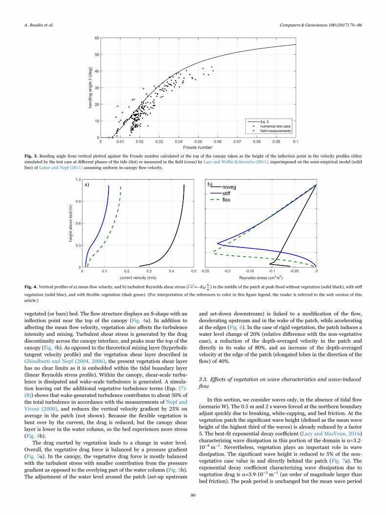
vegetated (or bare) bed. The flow structure displays an S-shape with aninflection point near the top of the canopy (Fig. 4a). In addition toaffecting the mean flow velocity, vegetation also affects the turbulenceintensity and mixing. Turbulent shear stress is generated by the dragdiscontinuity across the canopy interface, and peaks near the top of thecanopy (Fig. 4b). As opposed to the theoretical mixing layer (hyperbolictangent velocity profile) and the vegetation shear layer described inGhisalberti and Nepf (2004, 2006), the present vegetation shear layerhas no clear limits as it is embedded within the tidal boundary layer(linear Reynolds stress profile). Within the canopy, shear-scale turbu-lence is dissipated and wake-scale turbulence is generated. A simula-tion leaving out the additional vegetative turbulence terms (Eqs. (7)-(8)) shows that wake-generated turbulence contributes to about 50% ofthe total turbulence in accordance with the measurements of Nepf andVivoni (2000), and reduces the vertical velocity gradient by 25% onaverage in the patch (not shown). Because the flexible vegetation isbent over by the current, the drag is reduced, but the canopy shearlayer is lower in the water column, so the bed experiences more stress(Fig. 4b).

The drag exerted by vegetation leads to a change in water level.Overall, the vegetative drag force is balanced by a pressure gradient(Fig. 5a). In the canopy, the vegetative drag force is mostly balancedwith the turbulent stress with smaller contribution from the pressuregradient as opposed to the overlying part of the water column (Fig. 5b).The adjustment of the water level around the patch (set-up upstream

and set-down downstream) is linked to a modification of the flow,decelerating upstream and in the wake of the patch, while acceleratingat the edges (Fig. 6). In the case of rigid vegetation, the patch induces awater level change of 20% (relative difference with the non-vegetativecase), a reduction of the depth-averaged velocity in the patch anddirectly in its wake of 80%, and an increase of the depth-averagedvelocity at the edge of the patch (elongated lobes in the direction of theflow) of 40%.

3.3. Effects of vegetation on wave characteristics and wave-inducedflow

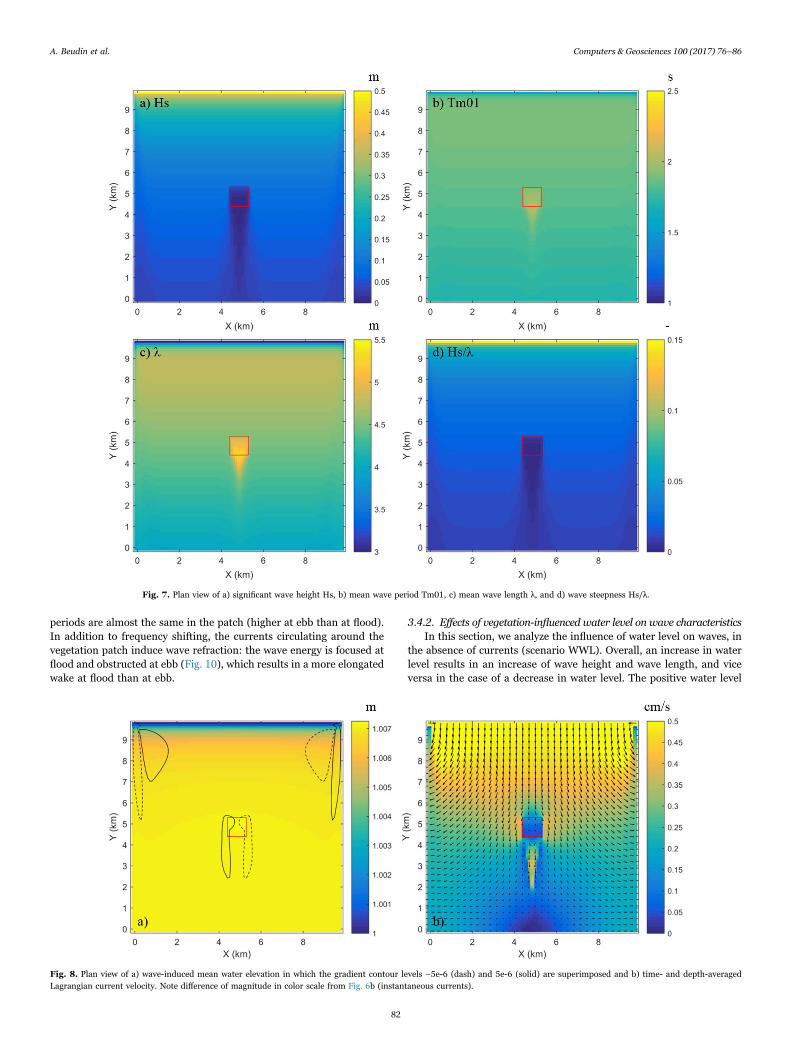
In this section, we consider waves only, in the absence of tidal flow(scenario W). The 0.5 m and 2 s waves forced at the northern boundaryadjust quickly due to breaking, white-capping, and bed friction. At thevegetation patch the significant wave height (defined as the mean waveheight of the highest third of the waves) is already reduced by a factor5. The best-fit exponential decay coefficient (Lacy and MacVean, 2016)characterizing wave dissipation in this portion of the domain is α=3.2·10−4 m−1. Nevertheless, vegetation plays an important role in wavedissipation. The significant wave height is reduced to 5% of the non-vegetative case value in and directly behind the patch (Fig. 7a). Theexponential decay coefficient characterizing wave dissipation due tovegetation drag is α=3.9·10−3 m−1 (an order of magnitude larger thanbed friction). The peak period is unchanged but the mean wave period

Fig. 3. Bending angle from vertical plotted against the Froude number calculated at the top of the canopy taken as the height of the inflection point in the velocity profiles eithersimulated by the test case at different phases of the tide (dot) or measured in the field (cross) by Lacy and Wyllie-Echeverria (2011), superimposed on the semi-empirical model (solidline) of Luhar and Nepf (2011) assuming uniform in-canopy flow velocity.

Fig. 4. Vertical profiles of a) mean flow velocity, and b) turbulent Reynolds shear stress (v w K′ ′=− Mδvδz) in the middle of the patch at peak flood without vegetation (solid black), with stiff

vegetation (solid blue), and with flexible vegetation (dash green). (For interpretation of the references to color in this figure legend, the reader is referred to the web version of thisarticle.)

A. Beudin et al. Computers & Geosciences 100 (2017) 76–86

80

increases up to 10% (Fig. 7b) and the mean wave length increases up to15% (Fig. 7c). This reduction in wave height and increase in wavelength result in a reduction of wave steepness (Fig. 7d), so thevegetation tends to smooth the sea surface locally and behind thepatch (glassy appearance observed in the field). As a corollary of wavedissipation, the presence of a vegetation patch induces sharp horizontalvariations in wave height responsible for wave directional spreading(diffraction effect).

As the wave energy (and momentum) flux decreases due to bottomfriction, the mean water level increases (setup) to balance. The patch ofvegetation dampens the wave-driven flow resulting in an additionalwave setup (Fig. 8a). Interestingly, the convergence of wave energy fluxbehind the vegetation patch generates an area of enhanced current(Fig. 8b). The magnitude of the wave-driven flow is much smaller thanthe tidal flow in this case, nevertheless these results give a sense of thequalitative influence of vegetation in wave-dominated environments.

3.4. Effects of vegetation-influenced tidal flow on wavecharacteristics

Tides influence wave characteristics by varying both current andwater depth. To isolate these two processes, we analyze sequentially the

outputs of two wave model runs: one with no water level fluctuation(scenario WC) and the other with the current set to zero (scenarioWWL).

3.4.1. Effects of vegetation-influenced currents on wave characteristicsIn this section, we analyze the effects of currents on waves, in the

absence of water level fluctuations (scenario WC). Overall, the wavesare bigger during flood tide than during ebb tide as the rate of waveenergy dissipation is reduced with a following (flood) current andincreased with an opposing (ebb) current (Figs. 9–10). This applies towave dissipation due to vegetation, reduced by 40% at flood andincreased by a factor two at ebb relative to the non-tidal case (Fig. 9b).Nevertheless, the significant wave height in the vegetation patch issmaller with flood current than with no current (Fig. 9a). It appearedthat the intrinsic/relative wave period is also reduced at flood(increased at ebb, not shown) forcing the wave height to decrease toconserve wave action density. This result agrees with Bacchi et al.(2014) who indicated that the damping by vegetation is more im-portant at higher wave frequencies. In addition, the apparent (abso-lute) wave period is also reduced at flood and increased at ebb as aresult of Doppler shift; the vegetation patch damps the current andtherefore attenuates this relativistic process: absolute and relative wave

Fig. 5. Cross-shore (along Y-axis) variation of momentum balance terms integrated over a) the water column and b) the canopy, in the middle of the domain in the case of stiffvegetation (fveg=vegetation drag, prsgrd=pressure gradient, bstr=bottom friction, vvisc=vertical viscosity, hadv=horizontal advection). Wave propagation is from the right of the figureto the left of the figure.

Fig. 6. Plan view of a) water level anomaly (relative difference between the stiff vegetation and the non-vegetation cases) and b) depth-averaged velocity, at peak flood. The patch of(stiff) vegetation is located in the red square. The hydrodynamic is forced at the northern boundary.

A. Beudin et al. Computers & Geosciences 100 (2017) 76–86

81

periods are almost the same in the patch (higher at ebb than at flood).In addition to frequency shifting, the currents circulating around thevegetation patch induce wave refraction: the wave energy is focused atflood and obstructed at ebb (Fig. 10), which results in a more elongatedwake at flood than at ebb.

3.4.2. Effects of vegetation-influenced water level on wave characteristicsIn this section, we analyze the influence of water level on waves, in

the absence of currents (scenario WWL). Overall, an increase in waterlevel results in an increase of wave height and wave length, and viceversa in the case of a decrease in water level. The positive water level

Fig. 7. Plan view of a) significant wave height Hs, b) mean wave period Tm01, c) mean wave length λ, and d) wave steepness Hs/λ.

Fig. 8. Plan view of a) wave-induced mean water elevation in which the gradient contour levels −5e-6 (dash) and 5e-6 (solid) are superimposed and b) time- and depth-averagedLagrangian current velocity. Note difference of magnitude in color scale from Fig. 6b (instantaneous currents).

A. Beudin et al. Computers & Geosciences 100 (2017) 76–86

82

anomaly upstream of the vegetation patch (Fig. 6a) allows the presenceof larger waves locally, and in the wake of the patch after propagation(Fig. 11a). For an opposite water level anomaly (down upstream and updownstream), the waves are smaller when they meet the patch, but theyare enhanced (compared to the constant water level case) in the wakeof the patch as a result of being less dampened in the patch (Fig. 11b).

3.5. Effects of vegetation-influenced waves on tidal flow

In this section, we analyze the influence of waves on tidal flow(scenario FW). The contribution of wave-forcing to the momentumbalance is negligible at flood in the cross-section shown in Fig. 5 (twoorders of magnitude less) but is manifest (10–20% increase in depth-averaged velocity) at the edge of the vegetation patch where the wave-induced Stokes flow interacts with strong flow vorticity, and as a resultthe lobes of maximum current velocity (Fig. 6b) are slightly shifted andmore elongated in the direction of wave propagation. While flow speedincreases on the lateral edges of the vegetation patch, it decreasesupstream by ~ 20%, above the vegetation patch by ~ 75%, and in the v-shaped wave wake downstream by ~ 35%. In the tide-only case(Fig. 6b), the flow speed was reduced by ~ 10, 80 and 20%, respectivelyacross the vegetation patch. Therefore, the capacity of vegetation toreduce the flow speed is enhanced in the presence of waves.

4. Discussion

4.1. Advancement of open-source modeling tools

Coastal storms are generally a combination of extreme water levels,strong winds, large waves, and intense rainfall. The simulation of theseevents require accounting for wind-wave-current interactions. TheCoupled Ocean-Atmosphere-Wave-Sediment Transport (COAWST)modeling system has been successfully applied under various stormconditions in several coastal and estuarine environments (e.g., Warneret al., 2010, Olabarrieta et al., 2011, Ralston et al., 2013). The wave-flow-vegetation module now allows for quantification of the effects ofemergent and submerged aquatic vegetation on storm surge, waves,and sediment transport, which can be used to inform ecosystem-basedcoastal risk management.

COAWST also integrates a coupled biogeochemical-optical modelbased on a nutrient, phytoplankton, zooplankton, and detritus model(Fennel et al., 2006) and a light attenuation model depending onconcentrations of suspended sediment, organic material, and phyto-plankton (del Barrio et al., 2014). The wave-flow-vegetation moduleprovides a new linkage for assessing the hydrodynamic forces on aseagrass bed and the resulting sediment resuspension and mixing inand above the seagrass canopy that affect light availability, and in turnpotential seagrass biomass production. Future versions of the code will

Fig. 9. Cross-shore (along Y-axis) variation of a) significant wave height and b) total wave energy dissipation in the middle of the domain at peak flood (blue), peak ebb (red), and withno tide (black). In the left panel, the dash lines are the results without vegetation. Wave propagation is from the right of the figure to the left of the figure. (For interpretation of thereferences to color in this figure legend, the reader is referred to the web version of this article.)

Fig. 10. Transport of wave energy during a) flood and b) ebb tides.

A. Beudin et al. Computers & Geosciences 100 (2017) 76–86

83

include above and below ground biomass changes to vegetation classesbased on light and nutrient availability.

4.2. Limitations and possible improvements

4.2.1. Calculation of bed shear-stressThe assumption of a logarithmic velocity profile near the bed is

questionable within the vegetation canopy as is the calculation of bedshear-stress. In particular, the model in its current state cannotrepresent the enhanced bed shear-stress in sparse canopy comparedto bare sediment that results in “sandification” (winnowing of mud) ofthe vegetated bed (Van Katwijk et al., 2010; Nepf, 2012). In addition tobed shear-stress partitioning to isolate the skin friction relevant tosediment transport, the calculation of the total bed shear-stress (dragform plus skin friction) should account for the contribution of thecanopy shear-stress and wake-generated turbulence. Although thenear-bed turbulent structure can be difficult to resolve with the verticalresolution used in coastal models, using the near-bed Reynolds stress(or the turbulent kinetic energy) instead of the vertical velocity gradientto calculate the total bed shear-stress could reproduce the density/flexibility dependent trend in bed shear-stress (Fig. 4b). As currentlyformulated, the model will represent the tendency for vegetated areasto trap sediment and reduce effective settling velocity, which is animportant bio-physical feedback in coastal systems.

4.2.2. Parameterization of flexible canopy motionsThe waving motions of flexible canopies, called monami when

following coherent eddies, decrease the amount of vertical momentumtransfer by up to 40% compared to rigid canopies (Ghisalberti andNepf, 2006). Several LES models have been designed to resolve theeddy structures in the vegetated shear layer and their coupling with theplant motions (e.g., Ikeda et al., 2001, Dupont et al., 2010), but to theauthors’ knowledge there is no existing eddy viscosity parameterizationaccounting for these interactions.

The wave dissipation due to vegetation term in SWAN currentlyneglects the plant swaying motion. Luhar and Nepf (2016) recentlyextended their effective blade length approach for steady-flow (Luharand Nepf, 2011) to unsteady-flows, accounting for plant flexibility andmotion in wave dissipation models. Their formulation will be imple-mented in COAWST along with expanding horizontally the dimensionof the vegetation height variable in SWAN. Nevertheless, furtherinvestigations remain ongoing regarding the flexible plant reconfigura-

tion under combined wave and current interactions.

4.2.3. Computational expense, obstacles and future considerationsWe compared the computational costs of using the vegetation

module relative to a simplified approach that uses bottom roughnessto account for increased drag in the model domain. The increase in thecomputational costs arises in different parts of the model, mainly in the2D and 3D kernels, and the GLS vertical mixing model which computesturbulent quantities (Table 2). Overall, the vegetation module increasescomputational costs by 6% over a run where the vegetation patch isrepresented by coarser sediment. The increase occurs from thecalculation of the vegetation drag and turbulence terms in the vegeta-tion module. These terms are then added to the 2D kernel, 3Dmomentum equations, and vertical mixing parameterization.

The implementation of this functionality in COAWST was met byseveral numerical and conceptual obstacles, which will require futureinvestigation and troubleshooting. For example, the ROMS hydrody-namic model required a reduced time step with the vegetation module(e.g. 1 s instead of 10 s) to eliminate instabilities resulting from sharpvelocity gradients. We also found that horizontal buoyancy and shearterms in the turbulence model needed to be unsmoothed to avoidperturbations at the corner of the vegetation patch. One possiblesolution is to gradually ramp up vegetation density into the patch,which can either be accomplished through modification of the initi-alization file, or through a coding modification. The SWAN modelcurrently does not account for multiple vegetation types, and does notdissipate wave energy (due to vegetation) spectrally; i.e. dissipation isapplied uniformly across the wave spectra. In the case of multiple

Fig. 11. a) Relative difference in significant wave height between the positive anomaly case (described in Fig. 6a) and the constant water level case, and b) cross-shore (along Y-axis)variation of significant wave height (in the middle of the domain) with a positive water level anomaly (blue), no anomaly (constant water level, black), and a negative anomaly (red). Thedash lines are the results with no wave dissipation due to vegetation. (For interpretation of the references to color in this figure legend, the reader is referred to the web version of thisarticle.)

Table 2Increase in computational expense due to implementation of the vegetation modulerelative as opposed to a simplified approach that uses bottom roughness to account forincreased drag. All times are in seconds, summed over 24 cpus.

Modelcomponent

Bottomroughness case

Vegetationmodule case

Increase incomputational time

Vegetationmodule

N/A 4310.716 N/A

2D kernel 108,442.567 113,364.426 4.53%GLS vertical

mixing18,379.465 20,150.028 9.63%

3D kernel 62,767.183 63,416.523 1.03%Total 192,294.957 203,947.535 6.14%

A. Beudin et al. Computers & Geosciences 100 (2017) 76–86

84

vegetation types an equivalent shoot density is defined in ROMS andSWAN. Future versions of SWAN will account for spatially-variableplant properties as in ROMS. Lastly, a systematic parameter studywould constrain the uncertainty of the numerous model parameteriza-tions implemented here. The development of this open-source tool willallow such studies to commence.

5. Summary and conclusion

We have developed a coupled wave-flow-vegetation module in theCOAWST modeling system applicable to vegetated flows in riverine,lacustrine, estuarine and coastal environments. New vegetative com-ponents were implemented in the flow model ROMS, namely plantposture-dependent three-dimensional drag, vertical mixing, and wave-induced streaming. The model reproduces key features of flow-vegeta-tion hydrodynamic interaction, in particular the strong shear layer atthe top of a submerged canopy which varies in height as the plantsbend. The coupling framework has also been updated to exchangevegetation-related variables between the flow and the wave modelSWAN to account for wave dissipation by vegetation in the presence ofcurrents and water level fluctuations. Results from the idealized testcase in shallow water highlight the nonlinear interdependency between(tidal) flow and wave characteristics in the presence of a vegetationpatch. In particular, the coupled wave-flow-vegetation model showsthat the vegetation modifies the wave characteristics (height, period,steepness, and direction) primarily by wave energy dissipation result-ing from the work done by drag force on the vegetation stems, andsecondarily by influencing the water level and current fields: i) any(positive or negative) gradient of free surface elevation across thevegetation patch reduces vegetation-induced wave damping; ii) wavedissipation rate decreases/increases when waves propagate along/against the current, while the (intrinsic) wave frequency increases/decreases to conserve wave action density which enhances/diminisheswave dissipation by bed friction and vegetation drag. In parallel, wavesinfluence the flow; therefore, waves alter the capacity of vegetation toreduce current speed and adjust water level. This model contributes toan improved understanding of how aquatic vegetation influences thephysical environment and, more generally, provides a multidisciplinarytool for informing decision-making of the potential ecologic andeconomic benefits of aquatic vegetation.

Acknowledgment

This study was part of the Estuarine Physical Response to Stormsproject (GS2-2D), supported by the Department of Interior HurricaneSandy Recovery program. This paper benefitted from discussions withAlfredo Aretxabaleta, Dan Nowacki and Heidi Nepf, and from theinternal review of Jessica Lacy. The model in its current state(COAWST v3.2) is freely available (http://woodshole.er.usgs.gov/operations/modeling/COAWST/index.html) and model developmentis being conducted as an open-source community effort. We encouragefeedback that will continue to add features and make the model morerobust as the community of users and developers grows.

References

Bacchi, V., Gagnaire, E., Durand, N., Benoit, M., 2014. Wave energy dissipation inTOMAWAC. Telemac & Mascaret User Club, Grenoble, France, 15–17 Oct 2014.

Barbier, E.B., Koch, E.W., Silliman, B.R., Hacker, S.D., Wolanski, E., Primavera, J.,Granek, E.F., Polasky, S., Aswani, S., Cramer, L.A., Stoms, D.M., Kennedy, C.J., Bael,D., Kappel, C.V., Perillo, G.M.E., Reed, D.J., 2008. Coastal ecosystem-basedmanagement with nonlinear ecological functions and values. Science 18, 321–323.

Booij, N., Ris, R.C., Holthuijsen, L.H., 1999. A third-generation wave model for coastalregions, Part I, model description and validation. J. Geophys. Res. C4 104,7649–7666.

Carr, J., D'Odorico, P., McGlathery, K., Wiberg, P., 2010. Stability and bistability ofseagrass ecosystems in shallow coastal lagoons: role of feedbacks with sedimentresuspension and light attenuation. J. Geophys. Res. 115, G03011.

Chen, S.-N., Sanford, L., Koch, E.W., Shi, F., North, E.W., 2007. A nearshore model toinvestigate the effects of seagrass bed geometry on wave attenuation and suspendedsediment transport. Estuaries Coasts 30 (2), 296–310.

Dalrymple, R.A., Kirby, J.T., Hwang, P.A., 1984. Wave diffraction due to areas of energydissipation. J. Waterw. Port., Coast. Ocean Eng. 110, 67–79.

de Vriend, H.J., 2006. Integrated research results on hydrobiosedimentary processes inestuaries: algorithm for vegetation friction factor. Defra R &D Technical ReportFD1905/TR3.

Dijkstra, J.T., Uittenbogaard, R.E., 2010. Modeling the interaction between flow andhighly flexible aquatic vegetation. Water Resour. Res. 46, W12547.

DijkstraJ.T., 2012. Macrophytes in estuarine gradients: flow through flexible vegetation(Ph.D. thesis), TU Delft, 119 p.

Dupont, S., Gosselin, F., Py, C., De Langre, E., Hemon, P., Brunet, Y., 2010. Modellingwaving crops using large-eddy simulation: comparison with experiments and a linearstability analysis. J. Fluid Mech. 652, 5–44.

Fennel, K., Wilkin, J., Levin, J., Moisan, J., O’Reilly, J., Haidvogel, D., 2006. Nitrogencycling in the middle Atlantic Bight: results from a three-dimensional model andimplications for the North Atlantic nitrogen budget. Glob. Biogeochem. Cycles 20,GB3007.

GanthyF., 2011. Rôle des herbiers de zostères (Zostera noltii) sur la dynamiquesédimentaire du Bassin d’Arcachon. (Ph.D. thesis), University of Bordeaux, 284 p.

Ghisalberti, M., Nepf, H.M., 2004. The limited growth of vegetated shear layers. WaterResour. Res. 40, W07502.

Ghisalberti, M., Nepf, H.M., 2006. The structure of the shear layer in flows over rigid andflexible canopies. Environ. Fluid Mech. 6, 277–301.

Haidvogel, D.B., Arango, H.G., Budgell, W.P., Cornuelle, B.D., Curchitser, E., Di Lorenzo,E., Fennel, K., Geyer, W.R., Hermann, A.J., Lanerolle, L., Levin, J., McWilliams, J.C.,Miller, A.J., Moore, A.M., Powell, T.M., Shchepetkin, A.F., Sherwood, C.R., Signell,R.P., Warner, J.C., Wilkin, J., 2008. Ocean forecasting in terrain-followingcoordinates: formulation and assessment of the regional ocean modeling system. J.Comput. Phys. 227 (7), 3595–3624.

Hemminga, M.A., Duarte, C.M., 2000. Seagrass Ecology. Cambridge University Press,Cambridge, UK.

Ikeda, S., Yamada, T., Toda, Y., 2001. Numerical study of turbulent flow and honami inand above flexible plant canopy. Int. J. Heat Fluid Flow 22, 252–258.

Jones, C.G., Lawton, J.H., Shachak, M., 1994. Organisms as ecosystem engineers. Oikos69 (3), 373–386.

Kombiadou, K., Ganthy, F., Verney, R., Plus, M., Sottolichio, A., 2014. Modelling theeffects of Zostera noltei meadows on sediment dynamics: application to the Arcachonlagoon. Ocean Dyn. 64, 1499–1516.

Kumar, N., Voulgaris, G., Warner, J.C., Olabarrieta, M., 2012. Implementation of thevortex force formalism in the coupled ocean-atmosphere-wave-sediment transport(COAWST) modeling system for inner shelf and surf zone applications. Ocean Model.47, 65–95.

Lacy, J.R., Wyllie-Echeverria, S., 2011. The influence of current speed and vegetationdensity on flow structure in two macrotidal eelgrass canopies. Limnol. Oceanogr.:Fluids Environ. 1, 38–55.

Lacy, J.R., MacVean, L.J., 2016. Wave attenuation in the shallows of San Francisco Bay.Coast. Eng. 114, 159–168.

Lapetina, A., Sheng, Y.P., 2014. Three-dimensional modeling of storm surge andinundation including the effects of coastal vegetation. Estuar. Coasts 37, 1028–1040.

Lapetina, A., Sheng, Y.P., 2015. Simulating complex storm surge dynamics: three-dimensionality, vegetation effect, and onshore sediment transport. J. Geophys. Res.120, 7363–7380.

Le Bouteiller, C., Venditti, J.G., 2014. Sediment transport and shear stress partitioning ina vegetated flow. Water Resour. Res. 51, 2901–2922.

Luhar, M., Coutu, S., Infantes, E., Fox, S., Nepf, H.M., 2010. Wave-induced velocitiesinside a model seagrass bed. J. Geophys. Res. 115, C12005.

Luhar, M., Nepf, H.M., 2011. Flow-induced reconfiguration of buoyant and flexibleaquatic vegetation. Limnol. Oceanogr. 56 (6), 2003–2017.

Luhar, M., Nepf, H.M., 2013. From the blade scale to the reach scale: A characterizationof aquatic vegetative drag. Adv. Water Res. 51, 305–316.

Luhar, M., Nepf, H.M., 2016. Wave-induced dynamics of flexible blades. J. Fluids Struct.61, 20–41.

MadsenO.S., 1994. Spectral wave–current bottom boundary layer flows. In: Proceedingsof the 24th International Conference on Coastal Engineering Research Council,Kobe, Japan, pp. 384–398.

Marjoribanks, T.I., Hardy, R.J., Lane, S.N., 2014. The hydraulic description of vegetatedriver channels: the weaknesses of existing formulations and emerging alternatives.WIREs Water 1, 549–560.

Maza, M., Lara, J.L., Losada, I.J., Ondiviela, B., Trinogga, J., Bouma, T.J., 2015. Large-scale 3-D experiments of wave and current interaction with real vegetation. Part 2:experimental analysis. Coast. Eng. 106, 73–86.

Mendez, F.M., Losada, I.J., 2004. An empirical model to estimate the propagation ofrandom breaking and nonbreaking waves over vegetation fields. Coast. Eng. 51,103–118.

Möller, I., Spencer, T., French, J.R., Legget, D.J., Dixon, M., 1999. Wave transformationover salt marshes: a field and numerical modeling study from Norfolk, England.Estuar. Coast. Shelf Sci. 49, 411–426.

Morin, J., M. Leclerc, M., Secretan, Y., Boudreau, P., 2000. Integrated two-dimensionalmacrophytes-hydrodynamic modelling. J. Hydraul. Res. 38, 163–172.

Morison, J.R., O’Brien, M.P., Johnson, J.W., Schaaf, S.A., 1950. The force exerted bysurface waves on piles. Pet. Trans. AIME 189, 149–154.

Nepf, H.M., Vivoni, E.R., 2000. Flow structure in depth-limited, vegetated flow. J.Geophys. Res. 105 (C12), 547–557.

Nepf, H.M., 2012. Flow and transport in regions with aquatic vegetation. Annu. Rev.

A. Beudin et al. Computers & Geosciences 100 (2017) 76–86

85

Fluid Mech. 44, 123–142.Olabarrieta, M., Warner, J.C., Kumar, N., 2011. Wave-current interaction in Willapa Bay.

J. Geophys. Res. 116, C12014.Paul, M., Bouma, T.J., Amos, C.L., 2012. Wave attenuation by submerged vegetation:

combining the effect of organism traits and tidal current. Mar. Ecol. Prog. Ser. 444,31–41.

Ralston, D.K., Warner, J.C., Geyer, W.R., Wall, G.R., 2013. Sediment transport due toextreme events: the Hudson River estuary after tropical storms Irene and Lee.Geophys. Res. Lett. 40, 5451–5455.

Ree, W.O., 1949. Hydraulic characteristics of vegetation for vegetated waterways. Agric.Eng. 30, 184–189.

Sheng, Y.P., Lapetina, A., Ma, G., 2012. The reduction of storm surge by vegetationcanopies: three‐dimensional simulations. Geophys. Res. Lett. 39 (20).

Soulsby, R.L., 1997. Dynamics of Marine Sands. Thomas Telford, London, 249.Suzuki, T., Zijlema, M., Burger, B., Meijer, M.C., Narayan, S., 2012. Wave dissipation by

vegetation with layer schematization in SWAN. Coast. Eng. 59 (1), 64–71.Temmerman, S., Bouma, T.J., Govers, G., Wang, Z.B., De Vries, M.B., Herman, P.M.J.,

2005. Impact of vegetation on flow routing and sedimentation patterns: three-dimensional modeling for a tidal marsh. J. Geophys. Res. 110, F04019.

Temmerman, S., Meire, P., Bouma, T.J., Herman, P.M.J., Ysebaert, T., de Vriend, H.J.,2013. Ecosystem-based coastal defence in the face of global change. Nature 504,79–83.

Uittenbogaard R., 2003. Modelling turbulence in vegetated aquatic flows. Internationalworkshop on RIParian Forest vegetated channels: hydraulic, morphological andecological aspects, Trento, Italy, 20–22 February 2003.

Umlauf, L., Burchard, H., 2003. A generic length-scale equation for geophysicalturbulence models. J. Mar. Res. 61, 235–265.

Van Katwijk, M.M., Bos, A.R., Hermus, D.C.R., Suykerbuyk, W., 2010. Sedimentmodification by seagrass beds: muddification and sandification induced by plantscover and environmental conditions. Estuar. Coast. Shelf Sci. 89, 175–181.

Warner, J.C., Sherwood, C.R., Arango, H.G., Signell, R.P., 2005. Performance of fourturbulence closure models implemented using a generic length scale method. OceanModel. 8, 81–113.

Warner, J.C., Sherwood, C.R., Signell, R.P., Harris, C.K., Arango, H.G., 2008a.Development of a three-dimensional, regional, coupled wave. Curr. Sediment-Transp. Model. Comput. Geosci. 34, 1284–1306.

Warner, J.C., Perlin, N., Skyllingstad, E.D., 2008b. Using the model coupling Toolkit tocouple earth system models. Environ. Model. Softw. 23, 1240–1249.

Warner, J.C., Armstrong, B., He, R., Zambon, J.B., 2010. Development of a coupled.Ocean Model. 35, 230–244.

Warner, J.C., Defne, Z., Haas, K., Arango, H.G., 2013. A wetting and drying scheme forROMS. Comput. Geosci. 58, 54–61.

Wu, W., 2014. A 3-D phase-averaged model for shallow-water flow with waves invegetated water. Ocean Dyn. 64, 1061–1071.

A. Beudin et al. Computers & Geosciences 100 (2017) 76–86

86