Contents lists available at ScienceDirect

Computers, Environment and Urban Systems

journal homepage: www.elsevier.com/locate/ceus

Data-driven analysis on the effects of extreme weather elements on trafficvolume in Atlanta, GA, USA

David Sathiaraja,⁎, Thana-on Punkasemb, Fahui Wangc, Dan P.K. Seedahd

a Dept of Geography and Anthropology and NOAA Southern Regional Climate Center, Louisiana State University, United StatesbDept. of Human Centered Design & Engineering, University of Washington, United Statesc Dept. of Geography and Anthropology, Louisiana State University, United Statesd Texas Transportation Institute, Texas A&M University, United States

A R T I C L E I N F O

Keywords:Weather hazardsTransportationUrban infrastructureClimateBig dataData analyticsMachine learningData visualization

A B S T R A C T

Severe weather events pose a significant threat to transportation networks. This research analyzes and discussesthe impact of precipitation, temperature, visibility and wind speed on hourly weekday traffic flow volume inAtlanta, Georgia. The study involves the following: determine weather variables that affect traffic volume, de-velop a machine learning technique to derive decision rules based on weather and traffic volume, and create aweb-based decision support visualization tool using the analyzed results. The relationship between extremeweather events and traffic volume was investigated by comparing traffic volume between a base case scenarioand an extreme weather scenario. Data from 48 Automatic Traffic Recorder (ATR) sites around Atlanta, GA, USAand hourly precipitation data from 4 climate measurement stations were used to conduct this study. The spa-tiotemporal relationships between traffic volume and weather variables were analyzed individually and eval-uated using a non-parametric statistical test. A machine learning technique is applied to derive decision rulesthat result in reduction in traffic volume. Results show significant impacts on traffic volume from visibility,precipitation and temperature and helps in isolating hours in a typical weekday when such impacts are felt. Adecision support tool was also developed to visualize traffic volume and weather interactions. The data-driveninsights from this analysis is applicable to transportation planners, centralized traffic control rooms and urbaninfrastructure decision makers.

1. Introduction

The transportation sector is an important component for the eco-nomic development of an area. An efficient transportation networkincreases economic and social opportunities by improving accessibilityto employment, markets, and additional investments. As populationand the number of vehicles increases, congestion on road networksbecomes more common. Traffic congestion accounts for over threebillion hours of traffic delay annually in the US (Press release - urbanmobility information, 2015).

Extreme weather events can adversely impact traffic volume (Cools,Moons, & Wets, 2010, Calvert & Snelder, n.d.). These weather eventshave negative effects on transportation network performance, travelspeed, time, capacity, and volume (Bartlett, Lao, Zhao, & Sadek, 2013).The Federal Highway Administration (FHWA) provided a statisticalreport showing that severe weather events cause up to 22% of vehicleaccidents. According to a 2015 Federal report (DoT, Nitch, Safety, &FLAP, 2015), more than 5897 deaths and 445,303 injuries occurred in

the U.S. during a ten-year period because of extreme weather events. Abetter understanding of weather factors affecting traffic flow caneventually help both government and other infrastructure agencies toproperly plan, design, and maintain road networks and thereby reducethe risk of fatalities.

This research investigates and analyzes the impact of four weathervariables - precipitation, visibility, temperature and wind speed - onhourly traffic volume. The focus of the study was on the city of Atlanta,Georgia, USA. One of the main motivations for choosing Atlanta was itbeing the large urban city with a dense transportation network and itspropensity to extreme weather hazards. NOAA climate normal reportsshow that Atlanta receives an average annual rainfall of 1262.63mm(49.71 in.) which is 27% more than the average in other similarly-sizedUS cities (Arguez et al., 2012).

Two major data sets were used in this research. Traffic data for thestate of Georgia, USA was provided by Transmetric LLC, a transporta-tion data management firm located in Austin, Texas. The weather datawas retrieved from the Integrated Surface Hourly (ISH) archives at the

https://doi.org/10.1016/j.compenvurbsys.2018.06.012Received 14 February 2018; Received in revised form 26 June 2018; Accepted 29 June 2018

⁎ Corresponding author at: E328 Howe Russell Bldg, NOAA Southern Regional Climate Center, Department of Geography, Louisiana State University, LA 70803, United States.E-mail address: davids@srcc.lsu.edu (D. Sathiaraj).

Computers, Environment and Urban Systems 72 (2018) 212–220

Available online 09 July 20180198-9715/ © 2018 Elsevier Ltd. All rights reserved.

T

National Centers for Environmental Information and housed locally.The impact of weather hazards on traffic volume was then studied

by applying rigorous statistical and machine learning tests. A decisionsupport tool was built to visualize the impacts of inclement weatherevents on transportation volume in Atlanta.

1.1. Problem description

This work focused on analyzing and examining the following re-search questions:

• Do precipitation, temperature, visibility and wind speed have asignificant impact on hourly traffic volume in Atlanta?

• If so, does the impact have a specific pattern? Is the impact differentbased on different times of the day and volumes of precipitation,temperature, visibility and wind speed?

• Is it possible to statistically correlate these impacts?

• Is it possible to develop a machine learning model that can accountfor interdependent weather variables and predict impacts on hourlytraffic volume?

1.2. Background and similar work

Previous studies examined relationships between weather eventsand traffic characteristics. A recent study by (Yuan-Qing & Jing, 2017)looked at the effect of rainfall on traffic flow on a freeway in Hainanprovince in China. Studies have shown that extreme weather conditionscould lead to reduction in speed, travel time, road capacity, and vo-lume. For instance, research from the Federal Highway Administrationshowed that light rainfall could reduce driving speed by 6–9% in sev-eral cities (Hranac et al., n.d.). This decrease in speed during extremeweather caused 3.5% more travel time compared to days (Stern, Shah,Goodwin, & Pisano, 2003) with normal weather conditions. Heavy rainhas been reported to produce a 14–15% reduction in traffic speed andcapacity (according to Agarwal, Maze, & Souleyrette (2005)), andheavy snow events have been reported to reduce the capacity of roadnetworks by up to 28% (Agarwal et al., 2005).

Some studies investigating traffic behavior using weather variableshave applied machine learning models to predict traffic characteristicsin different weather conditions. These machine learning models couldaccurately classify which variables contributed to change in trafficbehavior. For example, a study of the effect of traffic parameters onroad hazards using a classification tree model identified hazardous si-tuations on the freeways (Hasan, 2012). Results of this research showedthat traffic flow and vehicle speed were the most important factors thatinfluence traffic volume. Another study of the mixed effects of pre-cipitation on traffic crashes used a machine learning technique to builda crash risk prediction model based on precipitation and snowfall. Thestudy discovered that if precipitation increased by 10mm, the fatalcrash rate would increase about 3% (Eisenberg, 2004).

Previous research found decreases in traffic volume during differentsevere weather events. For example, an average winter storm event canreduce traffic volume by 29% (Knapp, Smithson, & Khattak, n.d.).Another urban study (Kwon, Fu, & Jiang, 2013) looked only at theimpact of winter weather conditions on traffic volume and the studymonitored just 2 locations over a 2 year period. A study used a prob-abilistic approach to find reductions in traffic volume during intensesnow and rain events (Samba & Park, 2010). A study of hourly trafficvolume and precipitation in Buffalo, NY, USA investigated relationshipsbetween traffic volume and precipitation by dividing traffic volumeinto two subgroups including 1) traffic volume during non-inclementweather (base case) and 2) inclement weather (inclement case) (Bartlettet al., 2013). This research applied a regression model to the dataset tocreate the predictive model under specific weather conditions. Resultsshowed a significant correlation between hourly rainfall and trafficvolume (Bartlett et al., 2013). Similarities between this study and that

of (Bartlett et al., 2013) were the sub-grouping of scenarios betweenextreme and normal weather conditions. The differentiating factorswere different cities with differing extreme weather thresholds, ana-lyzing a more extensive network of traffic counters, differing statisticaltechniques and use of a machine learning model to derive rules. Similarto our work, Angel, Sando, Chimba, & Kwigizile (2014) explored theeffect of rain on the traffic volume at 2 freeway sites in Florida andDehman & Drakopoulos (2017) studied the effect of inclement weatheron 15 freeway traffic counters in Milwaukee, Wisconsin. Factors thatdifferentiated our work were the extensive statistical analysis, the de-riving of thresholds and specific hours of affected traffic volume usingpredictive models and the decision support visualization tool.

Wind speed, temperature and visibility could also create hazardousdriving environments and cause a decrease in traffic volume. A study ofthe effect of wind speed, temperature, precipitation and visibility ontraffic capacity in Minnesota found that precipitation had the mostsevere impact on traffic capacity, reducing it by 19–28% (Agarwalet al., 2005). Cold temperatures and low visibilities had moderate im-pacts on the capacity, leading to a 10–12% decrease. However, windspeed did not have any noticeable effect on capacity reduction inMinnesota (Agarwal et al., 2005). Work such as Saha, Schramm, Nolan,& Hess (1994–2012) seek to provide a link between adverse weatherconditions with fatal vehicle crashes in the United States by looking atthe Fatality Analysis Reporting System (FARS) data set.

1.3. Outline

This work consists of three components. First, a statistical, data-intensive study is provided to analyze correlations between individualweather elements and traffic volume. Then, a machine learning modelis discussed to predict changes in traffic volume based on weatherconditions. Finally, a decision support tool is presented to visualizehourly traffic volume and its interaction with studied weather elements.

The paper is organized as follows: First, a background of prior re-search on this topic is provided. Also provided is a detailed descriptionof the datasets, along with methodologies pertaining to data collection,storage and data processing. Secondly, the statistical experiments andcomputational results are provided. Thirdly, a discussion of the ma-chine learning model and the development of the geo-visualizationdecision support tool (this includes programming methodologies used)is detailed. The last section provides conclusions and future work.

2. Study area and data processing

The focus area was the Atlanta Metropolitan Statistical Area (MSA)which has a dense network of traffic counting stations. Atlanta alsohappens to be an important business hub and one of the largest popu-lation centers in the southern U.S. According to the Georgia Departmentof Revenue, there are almost 3,000,000 personal passenger cars in thearea with nearly 500,000 daily riders. Weather hazards can play asignificant role in such a city.

The specific study area includes Cobb, Fulton, Dekalb, Henry andClayton counties (see Fig. 1). The study area covered approximately135mile2, containing latitudes between 33.4623° N and 34.0683° Nand longitudes between 84.1462° W and 84.6059° W. Based on theNOAA 1981–2010 US Climate Normals dataset (Arguez et al., 2012),this area averages 113 days with rain and 1263mm (49.7 in.) rainfallannually. The annual rainfall total is 27% larger than the averagerainfall in other cities with similar size across the United States. Pre-cipitation, visibility, wind speed and temperature data used was fromthe Integrated Surface Hourly (ISH) dataset (Smith et al. (2011)) of theNational Centers of Environmental Information (NCEI). ISH is a largehourly data set spanning more than 2000 stations worldwide. Fourweather measurement stations were available within the study area andreported regularly between 2010 and 2015 (see Fig. 1). The fourweather stations included: KATL (Hartsfield-Jackson Atlanta

D. Sathiaraj et al. Computers, Environment and Urban Systems 72 (2018) 212–220

213

International Airport), KFTY (Fulton County Airport-Brown Field),KPDK (Dekalb-Peachtree Airport) and KMGE (Dobbins Air ReserveBase). Spatial interpolation techniques such as Kriging, Inverse DistanceWeighting (IDW), and Radial Basis Functions (RBF) were then used tointerpolate weather observation values at each traffic counter location(see Fig. 1).

The study uses two main data sources: hourly traffic volume andweather variables. Hourly traffic volume data were collected from 48Automatic Traffic Recorder (ATR) sites spanning the 5-year period,2011–2015. The ATR stations are permanently installed sensors thatcount the number of vehicles passing through each counter location onstate highways, major county roads, and city streets on a 24/7/365 daybasis. The traffic dataset also consisted of information such as location(latitude and longitude) of the sites, names of the roads where eachcounter was located, amount of hourly traffic volume, and an hourlydate stamp that the counter recorded the traffic volume.

4 hourly weather elements/variables were examined: precipitation,visibility, wind speed and temperature. Weather data from theIntegrated Surface Hourly (ISH) data set of the National Centers ofEnvironmental Information (NCEI) was used. This analysis retrievednearly 225,000 records of hourly weather observations spanning thetime period, 2011–2015. Data was reported according to the UTCtimezone and were converted to US Eastern Time Zone (Atlanta's timezone).

2.1. Setting of parameters

This work analyzed only weekday traffic volume as weekday traffichas less variability than weekend traffic. Another aspect of our studywith regards to temperature was to only use data from the wintermonths of December to February. This was to isolate the study to aseason when such extreme temperatures are most likely to occur. Todetermine thresholds for the base and extreme cases, we use thresholdguidelines for climate extremes as suggested by the WorldMeteorological Organization (Data, 2009). As per the guidelines, a ty-pical threshold used is values above a certain percentile, 95th or 99th.In our study, we use values that are at the 99th percentile as a thresholdfor the extreme case. Since climate extremes vary from city to city, itwas appropriate to use a percentile-based threshold. Climate data fromthe 4 weather stations in the Atlanta area and for the 4 weather ele-ments were extracted. The 99th percentile values were then calculatedand used as a threshold to distinguish between the base and extremecases (and outlined in Table 1).

Table 2 provides a summary of average number of hours that fitunder the base condition category, the average number of hours that fitunder the extreme case category and the average percentage of extremeto base condition hours.

2.2. Spatial interpolation analysis

Since the data were collected at 4 unique climate measurementsites, spatial interpolation techniques such as Inverse DistanceWeighting (IDW), Kriging and radial basis functions (RBF) were used toestimate the 4 weather values at each of the 48 traffic counters. IDW(Mitas & Mitasova, 1999), Kriging (Hartkamp, De Beurs, Stein, & White,n.d.) and RBF (Rusu & Rusu, 2006) are commonly used spatial inter-polation techniques.

In order to find the most accurate spatial interpolation technique,data from the 4 weather stations in the study were spatially inter-polated. One of the weather stations was used as a reference station.The spatially interpolated values were then compared to the actualobserved values of the reference station and root-mean-square error(RMSE) values were calculated. The technique with the smallest RMSEvalue was used in the study.

Based on the RMSE results as reported in Table 3, IDW produced theleast error for precipitation, temperature, and visibility. However, for

Fig. 1. Map of counties. Map of Traffic sites. Map of climate sites.

Table 1Weather variable criteria used in the Atlanta transportation study.

Climate elements Base case Extreme case

Precipitation 0mm/h >7.62mm/hTemperature > 32 F ≤32 FWind Speed < 10m/s ≥10m/sVisibility > 5 km ≤5 km

Table 2Comparing of number of hours under base and extreme weather conditions in2011–2015 for the 48 Traffic Counters in Atlanta, GA.

Avg. base hours Avg. extreme hours Percent of extreme to base

Precipitation 33,467 2138 6.5Temperature 34,273 1047 3.5Wind Speed 34,461 222 0.7Visibility 33,216 1880 5.9

D. Sathiaraj et al. Computers, Environment and Urban Systems 72 (2018) 212–220

214

wind speed, RBF produced the smallest error compared to IDW andKriging. So IDW was used for interpolating temperature, rainfall andvisibility while RBF was used for spatial interpolation of wind speed.

3. Correlation analysis

After applying spatial interpolation techniques to get estimatedweather values at every traffic counter site, the next step was to findcorrelations between hourly traffic volume and hourly weather events.This was achieved for each traffic counter, by separating the trafficvolume data set on an hourly basis into base and extreme weather ca-tegories (using the thresholds outlined in Table 1.

A computational result of such a comparison is provided on anhourly basis for 2 traffic counters (with traffic counters # 36764 and#25065) in Figs. 2 and 3. The percentage drops in traffic volume causedby an extreme weather hazard is computed for each hour of a given day(see example computation in Table 4). It is also evident from Fig. 2 thaton certain hours of a day, there are substantial drops in traffic volumecaused by precipitation and temperature. For example, for precipita-tion, during the peak evening hours of 16 and 17 h, there is nearly a10% drop in traffic volume in Figs. 2 and 3.

To examine the influence of the 4 hazardous weather events ontraffic volume, the traffic dataset was divided into two subgroups - onecorresponding to hours that formed the base case (hours where therewere normal driving conditions with no extreme weather hazards) andanother corresponding to hours that experienced any or all of the 4extreme weather hazards. The base and extreme cases are categorizedin Table 1.

The 2 subgroups or time-series were created for each station. For thestatistical analysis, the hypothesis was that there was a difference

between the mean of hourly traffic volume in normal driving conditionsand the mean hourly traffic volume due to an extreme weather hazard.The non-parametric statistical test, Wilcoxon Test (Wilcoxon, 1945)was conducted on each of the 4 weather elements used in the study.

In many cases, due to the rarity of an extreme weather hazardnumbers of base cases outnumbered extreme cases more than fivetimes. To avoid issues from different sample sizes, a bootstrappingtechnique was used to randomly pick equal numbers of extreme andbase condition records and the statistical tests were repeated 100 times.The p-values were sorted in ascending order. After empirical analysis ofthe results and to ensure confidence in the repeatability of the results, p-values at the 80 percentile were chosen as representative of the group.If more than 80% of the p-value results fell under 0.05, it was inter-preted that there was a significant difference between the means of theextreme and base case scenarios.

4. Analysis of collective effect of weather variables on trafficvolume

To consider together all 4 weather elements and their collectiveeffect on traffic volume, we explore a predictive modeling and machinelearning technique, Random Forest (Breiman, 2001). In machinelearning, decision tree based learning involves the construction of a treelike structure to depict the features (or independent variables) in adataset. The constructed tree can help derive decision rules and forpredicting a target value. Decision trees can predict a categorical valuefor classification tasks (similar to this problem) or predict continuousvalues for regression. Decision trees use all the independent variables asinput and help provide decision rules with thresholds as an output. TheRandom Forest technique is an extension of the decision tree basedmethodology and involves the randomized construction of a number ofdecision trees and picking out the most commonly occurring treestructure for deriving decision rules. This technique finds applicabilityin areas such as behavioral science (Sathiaraj, Cassidy Jr., & Rohli,2017) and in transportation (Ghasri, Rashidi, & Waller, 2017). Machinelearning techniques such as Random Forest are also agnostic to theunderlying statistical distribution of the data set being analyzed. Thederived decision rules can help traffic planners and signal operators toknow thresholds and conditions when traffic volume will be belownormal and when it will be normal under abnormal weather conditions.

Table 3Root mean squared error (RMSE) values from each spatial interpolation tech-niques.

IDW Kriging RBF

Precipitation F8FF000.07596666 0.08476519 0.2435945Temperature F8FF001.778402 4.97 6.026029Visibility F8FF001.273612 1.49855 1.292256Wind speed 3.191654 3.201029 FFCCC9 3.124553

Fig. 2. Effect of different weather hazards on traffic volume by hour of day for station id 25065.

D. Sathiaraj et al. Computers, Environment and Urban Systems 72 (2018) 212–220

215

We derive predictive models for each of the traffic counters consideredin the study.

Previous research has applied entropy based decision trees to pre-dict climate events and traffic behavior. For example, one study used adecision tree classifier to predict precipitation in India. It showed thatthe decision tree learning approach provided an average accuracy of79.42% (Prasad, Reddy, & Naidu, n.d.). Another study used a decisiontree approach to analyze air traffic delay by comparing the accuracy ofresults from three machine learning models (Kulkarni, Wang, & Sridhar,2014). For this research, a decision tree based predictive technique isused to classify and predict as to which weather variables and theirthresholds, significantly contribute to the decrease of traffic volume.The predictive model splits the traffic dataset into a tree comprising of

nodes and branches (as depicted in Fig. 5). Training sets were generatedby classifying traffic volume into two categorical classes – normal andabnormal. For each traffic counter, the traffic volume that fell withinone standard deviation (spanning the time period 2011–2015), wasconsidered as the normal class, otherwise, it was considered as theabnormal class (or low traffic volume). The training data used were thehour of day, temperature, precipitation, visibility and wind speed. Foreach traffic counter, the data was normalized before a training set wasgenerated. A random forest decision tree model was then developed topredict the traffic volume case scenarios (normal vs abnormal). Themodels at each traffic counter averaged about 80–85% in predictiveaccuracy after a 10-fold cross-validation process.

An analysis of results is now described. First, the statistical analysisexamined the correlation between individual weather elements andtraffic volume. A machine learning model was built to analyze allweather elements simultaneously and to predict under which condi-tions traffic volume drops or stays normal. The decision support toolvisualized the interaction between weather elements and traffic volumeon an hourly and daily basis. Data from each traffic counter was splitinto base and extreme cases and then subjected to the Wilcoxon test.The statistical analysis was subjected to cross validation, the p-valuesfrom each dataset were then collected and analyzed graphically. TheWilcoxon test was chosen as it is a non-parametric test, suited forrandomly selected, paired samples and unlike the t-test, it does notassume that the underlying distribution is normally distributed.

Based on results from the Wilcoxon test, the effect of each weathervariable across all the traffic counters is plotted and depicted as Fig. 4.The graphic provides information on specific hours of a typical daywhen a weather variable can impact traffic volume and the number oftraffic counters where the decrease in traffic volume was statisticallysignificant. Effects of precipitation, temperature and visibility on trafficvolume were felt at a majority of the traffic counters during certainhours of the day. Precipitation events accounted for large decrease intraffic volume during afternoon to late night hours. During this periodof a typical day, more than 70% of traffic counters showed a significantdrop of traffic volume. Precipitation had a significant impact on thedecline of traffic volume for more than 95% of the traffic stationsduring hours 19–21.

Extreme temperature had a significant impact on almost all hours ofthe day during the winter months. Temperature accounted for a decline

Fig. 3. Effect of different weather hazards on traffic volume by hour of day for station id 36764.

Table 4Percentage drops in traffic volume ((base case-extreme case)/base case) under 4weather hazards for traffic counter 36764.

Hour Precipitation Temperature Wind Visibility

0 7.69 14.86 4.74 31.871 5.13 16.89 7.01 34.392 1.85 24.51 2.78 35.783 7.89 31.08 6.58 30.264 1.22 10.26 3.61 28.925 2.5 13.57 6.67 27.86 7.4 12.38 6.52 13.667 8.14 10.55 7.08 12.998 3.07 8.97 4.46 7.359 3.57 7.02 8.46 6.6610 2.74 6.54 5.46 10.9911 2.86 5.54 2.9 5.8512 4.88 5.83 2.32 7.5313 5.07 4.01 1.39 4.9614 5.24 3.76 0.58 3.4615 6.49 9.34 1.19 3.7916 8.7 9.41 0.45 5.8917 9.16 17.56 1.02 7.2718 4.69 22.46 −0.59 12.6819 6.48 21.91 1.71 14.6520 7.66 22.95 2.74 15.9221 7.69 43.65 2.69 19.6822 12.33 43.56 3.23 19.4223 8.45 46.68 5.96 16.82

D. Sathiaraj et al. Computers, Environment and Urban Systems 72 (2018) 212–220

216

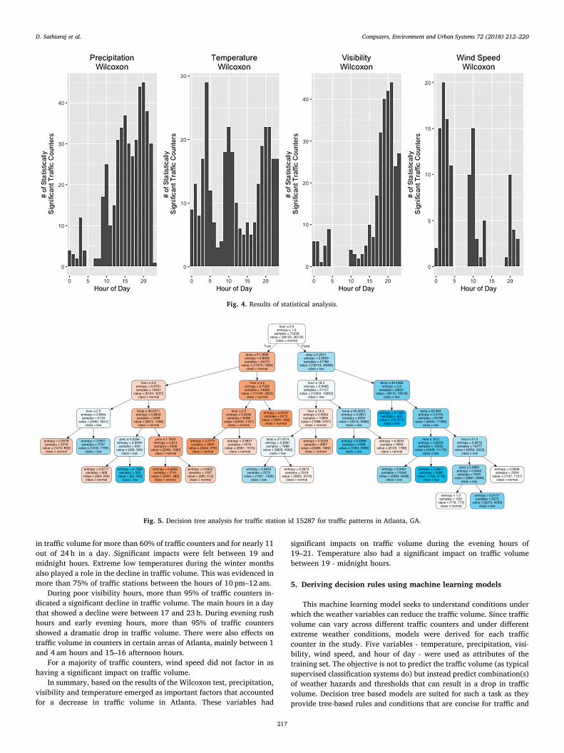
in traffic volume for more than 60% of traffic counters and for nearly 11out of 24 h in a day. Significant impacts were felt between 19 andmidnight hours. Extreme low temperatures during the winter monthsalso played a role in the decline in traffic volume. This was evidenced inmore than 75% of traffic stations between the hours of 10 pm–12 am.

During poor visibility hours, more than 95% of traffic counters in-dicated a significant decline in traffic volume. The main hours in a daythat showed a decline were between 17 and 23 h. During evening rushhours and early evening hours, more than 95% of traffic countersshowed a dramatic drop in traffic volume. There were also effects ontraffic volume in counters in certain areas of Atlanta, mainly between 1and 4 am hours and 15–16 afternoon hours.

For a majority of traffic counters, wind speed did not factor in ashaving a significant impact on traffic volume.

In summary, based on the results of the Wilcoxon test, precipitation,visibility and temperature emerged as important factors that accountedfor a decrease in traffic volume in Atlanta. These variables had

significant impacts on traffic volume during the evening hours of19–21. Temperature also had a significant impact on traffic volumebetween 19 - midnight hours.

5. Deriving decision rules using machine learning models

This machine learning model seeks to understand conditions underwhich the weather variables can reduce the traffic volume. Since trafficvolume can vary across different traffic counters and under differentextreme weather conditions, models were derived for each trafficcounter in the study. Five variables - temperature, precipitation, visi-bility, wind speed, and hour of day - were used as attributes of thetraining set. The objective is not to predict the traffic volume (as typicalsupervised classification systems do) but instead predict combination(s)of weather hazards and thresholds that can result in a drop in trafficvolume. Decision tree based models are suited for such a task as theyprovide tree-based rules and conditions that are concise for traffic and

Fig. 4. Results of statistical analysis.

Fig. 5. Decision tree analysis for traffic station id 15287 for traffic patterns in Atlanta, GA.

D. Sathiaraj et al. Computers, Environment and Urban Systems 72 (2018) 212–220

217

infrastructure planners to use and implement. Based on the decisiontree results from the model, hour of the day was a critical decisionmarker for deriving the decision rules, followed by temperature andprecipitation. An example of one such decision tree is provided fortraffic station 15287 as Fig. 5. The patterns of traffic volume weredifferent before and after the 10th hour. For hours prior to 10 am,temperature was the major variable that caused a drop in traffic vo-lume. Then, precipitation was the second leading cause for the declinein traffic volume. From Fig. 5, it is also evident, that traffic volumedrops when temperatures fall below 36 °F and precipitation is morethan 4mm per hour. However, for hours after 10 am, precipitationemerged as a significant variable. Temperature was the second mostimportant variable that led to the significant decreases in traffic vo-lume. During the hours after 10 am, traffic volume dropped drasticallywhen precipitation was more than 5mm per hour and temperature wasaround 33–35 °F.

In conclusion, after analyzing all variables together, precipitationand temperature were variables that greatly affected traffic volume inAtlanta. Wind speed did not emerge as a significant factor to cause adrop in traffic volume. Notably, the combination of temperature whenit was below 35 °F and precipitation that was more than 5mm/h cre-ated the most significant impact on traffic volume throughout the day.The predictive models also provided support to the notion (similar tothe results from the statistical analysis) that low temperatures duringthe early morning hours caused a decline in traffic volume (Fig. 5).

Based on the results from the statistical tests and the predictivemachine learning model, one can conclude that extreme precipitationand temperature (during the winter months) during certain hours of a

typical work day can negatively influence traffic volume. There weredifferent impact patterns among the weather elements. During mid-night to late morning hours in the winter months, extreme minimumtemperature in combination with poor visibility influences traffic vo-lume. Precipitation also contributed to a drop in traffic volume.Between noon and midnight, extreme precipitation was a significantfactor in decreasing traffic volume. For each traffic counter, the sta-tistical analysis yields specific hours when extreme weather hazards caninfluence a drop in traffic volume and the machine learning modelprovides combination(s) of weather conditions and their respectivethresholds under which traffic volume drops.

6. Technology stack and geo-visualization decision support tool

The technology behind the geo-visualization comprised of 3 com-ponents: a database to store the data, a front-end, interactive user in-terface for visualization of analytics, and a middle-layer web framework(Django, http://www.djangoproject.com) as a communication layerbetween the data base and the user-interface. The database used wasPostgresql http://www.postgresql.org and the front-end was written inJavascript and included the mapping library mapbox.js (http://mapbox.com) and the visualization library d3.js (http://d3js.org).

Geovisualization techniques were utilized to build a web-basedgeographic decision support tool. This tool was built to visually supportand provides a better understanding of the impact of hazardous weatherevents on traffic volume. The 5 main components of the geo-visuali-zation tool includes a map-based component, interactive displays fordaily and hourly traffic volume and comparative display of traffic

Fig. 6. A screenshot of the geo-visualization decision support tool.

D. Sathiaraj et al. Computers, Environment and Urban Systems 72 (2018) 212–220

218

volume under normal and extreme weather conditions.The map component displays the traffic counters used in the study

and allows a user to select a counter. Upon clicking a traffic counter, acalendar-based visualization is loaded that displays daily traffic volumeas a heat map. The calendar spans the 5 year study period. The heatmap is color-coded from red to green, red representing a daily trafficvolume that is 70% below the average traffic volume for that day from2011 to 2015. Dark green color is used when the daily traffic volume isgreater than or equal to the average traffic volume for that day across5 years. Yellow and light green are used for intermediary ranges. Whena user clicks a single day in the calendar, an hourly breakdown of trafficvolume is represented as a heat map with similar color codes as thedaily heat map.

The visualization tool also includes a chart-based representation ofthe analysis between the extreme and base cases of weather elements.When a user clicks on a weather element used in this study, 2 line chartsare loaded for a traffic counter. Each line chart spans a 24 hour windowin a day. The line charts depict traffic volume under extreme and baseweather conditions. The visualization enables a graphical depiction ofhours in a day when traffic volume is impacted by extreme weathercondition. The geographic information tool is available at http://wxtr.srcc.lsu.edu (screenshots of the tool have been included as Figs. 6 and7).

7. Conclusion

The impact of extreme weather elements - precipitation, minimumtemperature, visibility and wind speed - on hourly traffic volume wasanalyzed across 48 traffic counters in the city of Atlanta, Georgia, USA.This comprehensive, data-driven study comprised of analyzing theimpact of individual weather elements on traffic volume, developing apredictive machine learning model to predict conditions that caused thechange in traffic volume, and deriving a decision support tool to vi-sualize traffic volume and its interaction with the weather elements.

The influence of individual weather events on traffic volume wasstudied using the Wilcoxon test. Based on the statistical analysis, pre-cipitation, temperature and visibility emerged as factors that can causea significant decline in traffic volume. These weather elements had a

significant impact on traffic volume during the evening rush hour timesof 6–9 pm. Each weather variable indicated a decline in traffic volumeduring different hours of a typical week day. Temperature had thegreatest impact on traffic volume between 19 and 21 h in the wintermonths; precipitation indicated the most significant impact on trafficvolume between 13 and 22 h; and visibility had an impact on trafficvolume between 20 and 22 h. Overall, this approach of individuallyanalyzing historical weather data, enabled the isolation of hours in aweek day that are likely to be impacted in terms of traffic volume.These are depicted in the geo-visualization tool and enable trafficplanners and transportation officials in Atlanta to make appropriatepreparations in the event of extreme weather.

Predictive machine learning models were developed for each of thetraffic counters by considering all the weather hazard elements to-gether. This helping in deriving rules or conditions that includedcombination of weather hazard elements and under different thresh-olds. Temperature during the winter months and precipitation againemerged as influencing factors that reduced traffic volume. Winterprecipitation and extreme minimum temperature combined together tocause a decline in traffic volume. The predictive models were alsouseful in deriving decision rules that are useful for traffic managers andtransportation planners. The statistical analysis and the predictivemodels have helped derive specific hours in a typical week day duringwhich extreme weather conditions can severely affect traffic volume.The identification of weather element thresholds and affected hours hasapplications for efficient decision support and transportation planningacross major arteries in Atlanta's transportation network.

A decision support tool was created that provides easy access totraffic and weather data. The visualizations are useful for transportationplanners, traffic monitoring control rooms and urban planners to usethis information for facilitating smooth traffic flows and mitigatingbottlenecks caused by weather hazards. The geographic informationtool consists of components that help users understand the effect ofextreme weather elements on hourly and daily traffic volume. This toolalso depicted the comparison of traffic volume between normal andextreme weather conditions to show the hourly impact of each weathervariable on traffic volume. Results from this research could ultimatelyhelp transportation officials, stakeholders and planners in the overall

Fig. 7. Daily and hourly summary of traffic volume spanning 2010–2015 for a single traffic station in a calendar like view.

D. Sathiaraj et al. Computers, Environment and Urban Systems 72 (2018) 212–220

219

hourly assessment of extreme weather impacts on traffic volume inAtlanta, GA. Future work involves expanding the scope of the weatherelements and including winter elements such as snow and ice. Similarstudies such as this can also be undertaken for other large metropolitanareas and cities in the US.

References

Agarwal, M., Maze, T. H., & Souleyrette, R. (2005). Impacts of weather on urban freewaytraffic flow characteristics and facility capacity. Proceedings of the 2005 mid-continenttransportation research symposium18–19.

Angel, M. L., Sando, T., Chimba, D., & Kwigizile, V. (2014). Effects of rain on trafficoperations on Florida freeways. Transportation Research Record, 2440, 51–59. http://dx.doi.org/10.3141/2440-07.

Arguez, A., Durre, I., Applequist, S., Vose, R. S., Squires, M. F., Yin, X., ... Owen, T. W.(2012a). Noaa's 1981-2010 us climate normals: An overview. Bulletin of the AmericanMeteorological Society, 93(11), 1687–1697. http://dx.doi.org/10.1175/BAMS-D-11-00197.1.

Bartlett, A., Lao, W., Zhao, Y., & Sadek, A. W. (2013). Impact of inclement weather onhourly traffic volumes in buffalo, New York. Transportation Research Board 92ndannual meeting, no. 13-3240.

Breiman, L. (2001). Random forests. Machine Learning, 45(1), 5–32. http://dx.doi.org/10.1023/A:1010933404324.

S. C. Calvert, M. Snelder, Influence of weather on traffic flow: An extensive stochasticmulti-effect capacity and demand analysis, EUROPEAN TRANSPORT-TRASPORTIEUROPEI (Vol. 60).

Cools, M., Moons, E., & Wets, G. (2010). Assessing the impact of weather on traffic in-tensity. Weather Climate and Society, 2(1), 60–68. http://dx.doi.org/10.1175/2009WCAS1014.1.

Data, C. (2009). Guidelines on analysis of extremes in a changing climate in support ofinformed decisions for adaptation. http://www.wmo.int/pages/prog/wcp/wcdmp/wcdmp_series/, Accessed date: 16 May 2018.

Dehman, A., & Drakopoulos, A. (2017). How weather events affect freeway demandpatterns. Transportation Research Record, 2615, 113–122. http://dx.doi.org/10.3141/2615-13.

DoT, U., Nitch, D., Safety, M. R. A., & FLAP, A. I. (2015). Federal highway administration.Money, 103, 85–925.

Eisenberg, D. (2004). The mixed effects of precipitation on traffic crashes. AccidentAnalysis & Prevention, 36(4), 637–647.

Ghasri, M., Rashidi, T. H., & Waller, S. T. (2017). Developing a disaggregate travel de-mand system of models using data mining techniques. Transportation Research Part A-Policy and Practice, 105, 138–153. http://dx.doi.org/10.1016/j.tra.2017.08.020.

A. D. Hartkamp, K. De Beurs, A. Stein, J. W. White, Interpolation techniques for climatevariables.

Hasan, M. M. (2012). Investigation of the effect of traffic parameters on road hazard usingclassification tree model. International Journal for Traffic and Transport Engineering,2(3), 271–285.

R. Hranac, E. Sterzin, D. Krechmer, H. A. Rakha, M. Farzaneh, M. Arafeh, et al., Empiricalstudies on traffic flow in inclement weather.

K. Knapp, L. Smithson, A. Khattak, The mobility and safety impacts of winter storm eventsin a freeway environment, mid-continent transportation symposium 2000 proceed-ings, Iowa, USA.

Kulkarni, D., Wang, Y., & Sridhar, B. (2014). Analysis of airport ground delay programdecisions using data mining techniques. 14th AIAA aviation technology, integration, andoperations conference (pp. 2025). .

Kwon, T. J., Fu, L., & Jiang, C. (2013). Effect of winter weather and road surface con-ditions on macroscopic traffic parameters. Transportation Research Record, 2329,54–62. http://dx.doi.org/10.3141/2329-07.

Mitas, L., & Mitasova, H. (1999). Spatial interpolation, geographical information systems:Principles, techniques, management and applications. 1, 481–492.

N. Prasad, P. K. Reddy, M. M. Naidu, A novel decision tree approach for the prediction ofprecipitation using entropy in sliq, in: Computer modelling and simulation (UKSim),2013 UKSim 15th international conference on, IEEE, 2013, pp. 209–217.

Press release - urban mobility information. https://mobility.tamu.edu/ums/media-information/press-release/, Accessed date: 5 February 2018.

Rusu, C., & Rusu, V. (2006). Radial basis functions versus geostatistics in spatial inter-polations. Artificial intelligence in theory and practice (pp. 119–128). Springer.

Saha, S., Schramm, P., Nolan, A., & Hess, J. (1994-2012). Adverse weather conditions andfatal motor vehicle crashes in the United States. Environmental Health, 15. http://dx.doi.org/10.1186/s12940-016-0189-x.

Samba, D., & Park, B. B. (2010). Probabilistic modeling of inclement weather impacts ontraffic volume. Transportation Research Board 89th annual meeting, no. 10-0646.

Sathiaraj, D., Cassidy, W. M., Jr., & Rohli, E. (2017). Improving predictive accuracy inelections. Big Data, 5(4, SI), 325–336. http://dx.doi.org/10.1089/big.2017.0047.

Smith, A., Lott, N., & Vose, R. (2011). The integrated surface database: Recent develop-ments and partnerships. Bulletin of the American Meteorological Society, 92(6),704–708. http://dx.doi.org/10.1175/2011BAMS3015.1.

Stern, A. D., Shah, V., Goodwin, L., & Pisano, P. (2003). Analysis of weather impacts ontraffic flow in metropolitan, Washington DC. Proceedings of the 19th internationalconference on interactive information and processing systems (IIPS) for meteorology,oceanography, and hydrology.

Wilcoxon, F. (1945). Individual comparisons by ranking methods. Biometrics Bulletin,1(6), 80–83.

Yuan-Qing, W., & Jing, L. (2017). Study of rainfall impacts on freeway traffic flowcharacteristics. Transportation Research Procedia, 25, 1533–1543.

D. Sathiaraj et al. Computers, Environment and Urban Systems 72 (2018) 212–220

220