computers and fluids - university of delaware
TRANSCRIPT

Computers and Fluids 155 (2017) 9–21
Contents lists available at ScienceDirect
Computers and Fluids
journal homepage: www.elsevier.com/locate/compfluid
DUGKS simulations of three-dimensional Taylor–Green vortex flow
and turbulent channel flow
Yuntian Bo
a , Peng Wang
b , Zhaoli Guo
b , Lian-Ping Wang
b , c , ∗
a Department of Energy and Resource Engineering, Peking University, Beijing, PR China b State Key Laboratory of Coal Combustion, Huazhong University of Science and Technology, Wuhan, P.R. China c Department of Mechanical Engineering, 126 Spencer Laboratory, University of Delaware, Newark, Delaware 19716-3140, USA
a r t i c l e i n f o
Article history:
Received 3 March 2016
Revised 10 February 2017
Accepted 6 March 2017
Available online 7 March 2017
Keywords:
Discrete unified gas kinetic scheme
Lattice Boltzmann equation
Pseudo-spectral methods
3D Taylor–Green vortex flow
Turbulent channel flow
a b s t r a c t
The discrete unified gas-kinetic scheme (DUGKS) is a relatively new, finite-volume formulation of the
Boltzmann equation. It has several advantages over the lattice Boltzmann method (LBM) in that it can
naturally incorporate multiscale physical processes and non-uniform lattice mesh. With the goal of simu-
lating a variety of turbulent flows, we investigate two aspects of DUGKS. First, we explore a parallel im-
plementation strategy of DUGKS using domain decomposition and MPI (Message Passing Interface), and
demonstrate the scalability of the parallel DUGKS code. We validate the resulting parallel code using the
3D Taylor-green vortex flow where small eddies are generated over time from large eddies. The DUGKS
results are compared to short-time analytical solution as well as to those from LBM and pseudo-spectral
method. The second-order accuracy of DUGKS is confirmed by using the highest-resulotion DUGKS flow
as the benchmark. Second, we consider how to incorporate solid walls and non-uniform mesh in DUGKS
for three-dimensional flows, by simulating a turbulent channel flow. The statistics of the simulated turbu-
lent channel flow are compared to those based on LBM and spectral methods. It is found that the DUGKS
results, even with a coarse non-uniform mesh, are overall better than the LBM results when compared to
the spectral benchmark data.
© 2017 Elsevier Ltd. All rights reserved.
1
(
a
t
A
i
r
t
fl
w
fl
o
a
p
t
l
L
v
N
t
t
a
T
t
K
n
K
e
d
s
a
m
s
h
0
. Introduction
One of the major advances in computational fluid dynamics
CFD) in the last three decades is the emergence, development, and
pplications of mesoscopic numerical methods based on solving
he kinetic Boltzmann equation with a linearized collision model.
s the most popular mesoscopic method for simulating nearly
ncompressible flows, the lattice Boltzmann method (LBM) has
eceived a great deal of attention due to its simplicity, high compu-
ational efficiency, and capability of treating a variety of complex
ows such as flows through porous media, multiphase flows
ith moving fluid-fluid or fluid-solid interfaces, and turbulent
ows [1–7] . Although its spatial accuracy is of only the second-
rder, the low numerical dissipation of LBM [8,9] makes LBM
competitive CFD tool for simulating turbulent flows, and its
hysical accuracy has been demonstrated by comparing with
he N-S based pesudo-spectral methods [7,10,11] . The reason for
ow numerical dissipation in LBM is the accurate treatment (by
∗ Corresponding author.
E-mail addresses: [email protected] (Y. Bo), [email protected]
(P. Wang), [email protected] (Z. Guo), [email protected] (L.-P. Wang).
d
t
o
p
ttp://dx.doi.org/10.1016/j.compfluid.2017.03.007
045-7930/© 2017 Elsevier Ltd. All rights reserved.
agrangian streaming) of the advection term. Unlike the con-
entional CFD methods which solve the strongly nonlinear
avier–Stokes equations, the LBM solves essentially a linear equa-
ion with local nonlinearity residing in its collision term. In LBM,
he space and time discretizations are fully coupled to each other
nd to a highly symmetric set of discrete kinetic particle velocities.
his highly efficient treatment, however, constrains the method
o nearly incompressible flow under the continuum limit ( i.e. ,
nudsen number less than 10 −3 ) or, through extensions, to weak
onequilibrium flows [12–15] .
More general kinetic schemes that can handle flows at all
nudsen numbers have also been developed in parallel. A great
xample is the unified gas kinetic scheme (UGKS) [16,17] which is
esigned as a multiscale simulation tool that can treat, within a
ame framework, both the continuum limit (i.e., the N-S equations)
nd the free-molecular limit [18] . In this framework, the physical
odeling is directly performed at the scales of the spatial mesh
ize and time step size, with the use of a sufficient number of
iscrete kinetic velocities. The collisions of kinetic particles within
he grid volume and the particle transport through the surfaces
f the grid volume together determine the time evolution of the
article distribution functions.
10 Y. Bo et al. / Computers and Fluids 155 (2017) 9–21
2
l
fl
t
c
ξ
w
i
fi
w
f
u
e
t
t
l
a
t
E
(
m
t
t
e
e
b
o
w
a
n
H
t
B
�
w
∂
s
t
�
I
c
�
Recently, a discrete unified gas kinetic scheme (DUGKS)
[19,20] has been developed, combining the advantages of both LBM
and UGK S methods. DUGK S is designed as a finite-volume scheme
with flexible mesh adaptation. The key is the improved imple-
mentation of the calculations of surface transport fluxes through a
transformation of the distribution function coupled with the effect
of particle collisions. By using extended equilibrium distributions,
DUGKS has been shown to be capable of simulating flows at all
Knudsen numbers including thermal compressible flows [20] and
Boussinesq flows [21] . This greatly extends the potential applica-
tions of discrete-velocity based mesoscopic schemes.
A potential application of DUGKS is direct numerical simula-
tion of complex turbulent flows. Due to its finite-volume formu-
lation and its feasibility of incorporating unstructured mesh [22] ,
DUGKS could be potentially more efficient in treating inhomoge-
neous and wall-bounded turbulent flows. For laminar flow sim-
ulations, DUGKS has been shown to have a similar accuracy as
LBM [23] , but DUGKS is numerically much more stable when the
flow is under-resolved. For three-dimensional time-dependent tur-
bulent flows, a first comparative study of DUGKS and LBM was re-
ported by Wang et al. [24] , who concluded that DUGKS is capable
of simulating decaying homogeneous isotropic turbulence, but is
slightly more dissipative when compared to LBM. We must note
that DUGKS does not employ the usual finite-volume formulation
for the advection term. The novelty of DUGKS is that the flux at
the cell interface is computed using the distribution functions that
couple the advection and collision, namely, the flux is evaluated
by solving the Boltzmann evolution equation rather than by inter-
polation. This coupling strategy in DUGKS ensures low numerical
dissipation, as demonstrated in [25,26] . More specifically, in our
recent paper [24] , we show that DUGKS is capable of simulating
a decaying turbulent flow (without walls) and the resolution re-
quirement ( k max η > 3 ) for DUGKS is only slightly higher than that
for LBM ( k max η > 2 ), where k max and η are the largest wavenum-
ber resolved and the flow Kolmogorov length, respectively.
A critical step in extending the DUGKS applications to three-
dimensional turbulent flows is the scalable implementation. In this
paper, we report a first parallel implementation of DUGKS using
domain decompositions. The resulting parallel code is then vali-
dated using the three-dimensional energy-cascading Taylor–Green
vortex flow for which a short-time analytical solution exists. Com-
parisons with pseudo-spectral simulation results and LBM results
are also provided. Furthermore, we will demonstrate, for the first
time, a successful DUGKS simulation of a turbulent channel flow
using a relative coarse non-uniform mesh. It should be noted that
the efficient parallel implementations of LBM have been widely
studied, taking advantage of the strict local data communication
in LBM. The key is to explore the best use of data structure and
cache memory, and several implementation methods are available
[27–32] . The nature of data communication in DUGKS depends on
the exact algorithm used to compute the surface transport fluxes.
The remainder of the paper is organized as follows. In Section 2 ,
the basic algorithm of DUGKS is described, along with parallel im-
plementation details. The treatment of no-slip boundary and the
formulation of mesoscopic forcing are also developed. The numer-
ical results and scalability data are presented in Section 3 . Conclu-
sions and future outlook are given in Section 4 .
2. The DUGKS algorithm and parallel implementation
In this section, we describe the basic DUGKS algorithm, the
method to parallelize the code, and implementation of the non-
uniform, time-dependent forcing.
.1. The DUGKS algorithm
DUGKS begins with the Boltzmann equation with the BGK col-
ision model. In this paper, we only consider the incompressible
ow limit or flows with a small Mach number [19,23] . In this case,
he same discrete kinetic velocities used in the D3Q19 LBM model
an be adopted in DUGKS, namely,
α =
⎧ ⎨
⎩
( 0 , 0 , 0 ) c, α = 0
( ±1 , 0 , 0 ) c, ( 0 , ±1 , 0 ) c , ( 0 , 0 , ±1 ) c , α = 1 − 6
( ±1 , ±1 , 0 ) c, ( ±1 , 0 , ±1 ) c , ( 0 , ±1 , ±1 ) c , α = 7 − 18
(1)
here the speed of the sound is c =
√
3 RT , R is the gas constant, T
s the temperature. The discrete distribution function f α( x , t ) satis-
es the following equation,
∂ f α
∂t + ξα · ∇ f α = �α ≡ f (eq )
α − f α
τ+ �α, (2)
here τ is the relaxation time and �α denotes the mesoscopic
orcing used to represent the local nonuniform force F ( x , t ) per
nit volume in the Navier–Stokes equation.
At this point, we recall that the discrete-velocity Boltzmann
quation with the BGK collision model is designed to reproduce
he Navier–Stokes equations, by expanding the distribution func-
ion in terms of a set of Hermite ortho-normal polynomials in ve-
ocity space. This expansion allows the distribution function to be
pproximated in terms of conservative hydrodynamic variables and
heir derivatives [15] . With the BGK collision model, the Chapman–
nskog procedure implies that the continuity and Navier–Stokes
i.e. , macroscopic) equations depend only on a few leading mo-
ents of the distribution function instead of the full form of
he distribution function. Therefore, truncation of the higher-order
erms in the Hermite expansion of the distribution function has no
xplicit effect on the macroscopic equations [15] . Specifically, the
xplicit Hermite expansion of the Maxwelliam equilibrium distri-
ution at low Mach number (or isothermal limit), up to the second
rder in the Hermite expansion, is [15]
f (eq ) α = ρW α
[
1 +
ξα · u
RT +
(ξα · u
)2
2(RT ) 2 − u · u
2 RT
]
, (3)
here the weighting coefficients W α are W 0 = 1 / 3 , W 1 , ··· , 6 = 1 / 18 ,
nd W 7 , ··· , 18 = 1 / 36 ; ρ is the fluid density; and u is the hydrody-
amic fluid velocity.
The body force term should be formulated in the spirit of the
ermite approximation. According to the original Boltzmann equa-
ion, the forcing term � in the continuous-velocity form of the
oltzmann equation is [15,33]
(x , ξ, t) = −F j
ρ
∂ f (x , ξ, t)
∂ ξ j
, (4)
here f ( x, ξ, t ) is the continuous distribution function. The term
f ( x, ξ, t )/ ∂ ξj should be projected onto the truncated Hermite ba-
is. Shan et al. [15] showed explicitly, using our notations and up
o the second order in the Hermite expansion, that
α =
F j W α
RT
[(ξα, j − u j
)+ ξα, j
ξα · u
RT
]. (5)
n view of the leading-order terms in f (eq ) α , the above formulation
an be written alternatively as
α =
F j
ρ
[ (ξα, j − u j
)RT
f (eq ) α + O
(u
2 )]
≈F ·
(ξα, j − u j
)ρRT
f (eq ) α . (6)
Y. Bo et al. / Computers and Fluids 155 (2017) 9–21 11
T
t
s
E
m
�
T∑
w
f
s
m
ρ
o
o
m
s
t
s
t
w
d
o
f
w
T
f
a
Q
w
o
x
0
e
t
w
c
w
I
a
b
p
t
p
p
w
f
t
w
I
t
a
c
a
ρ
ρ
T
n
c
w
E
t
d
he O
(u
2 )
error term in Eq. (6) leads to an error of order O
(u
3 )
in
he Navier–Stokes equation, which is usually ignored under the as-
umption of low Mach number. It is noted that the approximation,
q. (6) , can also be derived if we start with Eq. (4) and approxi-
ate ∂ f / ∂ ξ j by ∂ f ( eq ) / ∂ ξ j [15,33] . We now write
α(x , t) ≈ φα f (eq ) α (x , t) , with φα ≡ F j ( ξα, j − u j )
ρRT . (7)
he consistency with the Navier–Stokes equations requires
α
�α = 0 , ∑
α
ξα, j �α = F j ,
∑
α
ξα, j ξα,k �α = u j F k + u k F j + O
(u
3 ), (8)
hich can be easily shown to be satisfied by the two alternative
orms, Eq. (5) and Eq. (7) . This consistency has also been demon-
trated in the LBM framework in [6] .
The hydrodynamic variables, namely, density ρ , the fluid
acrosopic velocity u , and pressure p are obtained as
=
∑
i
f α, ρu =
∑
α
ξα f α, p = ρRT . (9)
The DUGKS algorithm makes use of a finite-volume formulation
f Eq. (2) [19,20] . The advection term in Eq. (2) is treated as sum
f surface fluxes after applying the divergence theorem. This treat-
ent allows the lattice velocities to be decoupled from the grid
tructure. For the time integration, the collision term is treated by
he trapezoidal rule, similar to the lattice Boltzmann method. The
urface flux terms by the midpoint rule (other alternative formula-
ions may be used). The details are now explained below.
Consider here a cuboid grid cell centered at x i, j, k ≡ ( x i , y j , z k ),
ith cell sizes �x i , �y j , and �z k , respectively, in the x, y , and z
irections. The time evolution of the discrete distribution averaged
ver the cell volume V i, j,k = �x i �y j �z k , f α( x i, j, k , t ), is advanced
rom t = t n to t = t n +1 as,
˜ f α(x i, j,k , t n +1 ) =
˜ f + α (x i, j,k , t n ) −�t
V j
Q α(x i, j,k , t n +0 . 5 ) , (10)
here, for convenience, the transformed variables are defined as
˜ f α = f α − �t
2
�α, ˜ f + α = f α +
�t
2
�α. (11)
he code computes mainly the transformed variable ˜ f α, all other
orms of the distribution function can be expressed in terms of ˜ f αnd f
(eq ) α , as shown below.
The net flux Q α(x i, j,k , t n +0 . 5 ) is defined as
α(x i, j,k , t n +0 . 5 ) dS =
∫ ∂V j
(ξα · n
)f α(x b , t n +0 . 5 )
=
[f α(x i + , j,k , t n +0 . 5 ) − f α(x i −, j,k , t n +0 . 5 )
]ξα,x �y j �z k
+
[f α(x i, j+ ,k , t n +0 . 5 ) − f α(x i, j−,k , t n +0 . 5 )
]ξα,y �x i �z k
+
[f α(x i, j,k + , t n +0 . 5 ) − f α(x i, j,k −, t n +0 . 5 )
]ξα,z �x i �y j , (12)
here f α(x b , t n +0 . 5 ) is the distribution at the cell boundary
r interface x b at the half time step, x i + , j,k = x i, j,k + 0 . 5�x i e x ,
i −, j,k = x i, j,k − 0 . 5�x i e x , x i, j+ ,k = x i, j,k + 0 . 5�y j e y , x i, j−,k = x i, j,k − . 5�y j e y , x i, j,k + = x i, j,k + 0 . 5�z k e z , x i, j,k − = x i, j,k − 0 . 5�z k e z , and
x , e y , e z are unit vectors in x, y , and z directions, respectively.
The key step is then to properly evaluate F α . In DUGKS, after in-
egrating Eq. (2) along a particle path from t n to t n + h ( h ≡ 0.5 �t )
ith the collision term included, the distribution function at the
ell boundary at t n + h can be written as
f α(x b , t n + h ) = f + α (x b − h ξα, t n ) , (13)
here a second set of transformed variables are defined as
f α = f α − h
2
�α, f + α = f α +
h
2
�α. (14)
t is important to note that the evolution equation, Eq. (13) , is ex-
ct, namely, no numerical dissipation is introduced at this stage
etween two different times, t n and t n + h . Next, we need an ap-
roximation of f + α (x b − h ξα, t n ) at a single time t n using spatial in-
erpolation. There are many possibilities, such as the spectral inter-
olation or high-order compact finite-difference schemes. For sim-
licity, here we choose to utilize a local Taylor expansion, namely,
f α(x b , t n + h ) = f + α (x b − h ξα, t n ) ≈ f
+ α (x b , t n ) −h ξα · ∇ f
+ α (x b , t n ) ,
(15)
here f + α (x b , t n ) and its gradients ∇ f
+ α (x b , t n ) at the cell inter-
aces can be approximated by the second-order linear interpola-
ions from values at the cell centers. For example,
∂ f + α (x i + , j,k , t n )
∂x ≈ f
+ α (x i +1 , j,k , t n ) − f
+ α (x i, j,k , t n )
x j+1 − x j
=
f + α (x i +1 , j,k , t n ) − f
+ α (x i, j,k , t n )
(�x i + �x i +1 ) / 2
, (16a)
f + α (x i + , j,k , t n ) ≈ f
+ α (x i, j,k , t n ) +
∂ f + α (x i + , j,k , t n )
∂x
�x i 2
, (16b)
here
f + α
(x i, j,k , t n
)=
2 τ − h
2 τ + �t ˜ f α
(x i, j,k , t n
)+
(3 h
2 τ + �t +
3 hτ
2 τ + �t φα
)f (eq ) α
(x i, j,k , t n
). (17)
n Eq. (13) , the half time step values at the cell interface included
he particle collision effect. This coupled treatment of advection
nd collision makes DUGKS a self-adaptive scheme for both the
ontinuum regime and the free-molecular regime [19] .
Clearly, the hydrodynamic variables can also be evaluated using
ny of the transformed distributions, namely,
=
∑
α
˜ f α =
∑
α
˜ f + α =
∑
α
f α =
∑
α
f + α , (18a)
u =
∑
α
ξα˜ f α +
dt
2
F =
∑
α
ξα˜ f + α − dt
2
F =
∑
α
ξα f α +
h
2
F
=
∑
α
ξα f + α − h
2
F . (18b)
herefore, ρ(x b , t n + h ) and u (x , t n + h ) can be obtained from
f α(x b , t n + h ) , which can be used to compute f (eq ) α (x b , t n + h ) . Fi-
ally, the desired distributions at half time step at the cell interface
an be readily obtained by
f α( x b , t n + h ) =
2 τ
2 τ + h
f α(x b , t n + h )
+
(h
2 τ + h
+
τh
2 τ + h
φα
)f (eq ) α (x b , t n + h ) . (19)
hich can be used to compute the net flux F α(x i, j,k , t n + h ) using
q. (12) . This then allows the distribution function to be advanced
hrough Eq. (10) .
In the above formulation, we have defined five sets of discrete
istributions: f α, ˜ f α, ˜ f + α , f α, f + α . Any one of the five can be used to

12 Y. Bo et al. / Computers and Fluids 155 (2017) 9–21
i
-
u
b
u
1
h
p
r
t
c
i
s
t
l
o
D
s
l
i
2
c
w
v
s
s
H
l
p
t
w
i
d
w
i
a
t
t
e
3
l
s
p
[
T
3
a
S
c
u
determine the equilibrium distribution f (eq ) α and then the remain-
ing four. The most convenient choice is to follow the evolution of˜ f α, which can be used to determine others as follows [19]
f α =
2 τ
2 τ + �t ˜ f α +
(�t
2 τ + �t +
τ�t
2 τ + �t φα
)f (eq ) α , (20a)
f α =
2 τ + h
2 τ + �t ˜ f α +
(h
2 τ + �t +
τh
2 τ + �t φα
)f (eq ) α , (20b)
˜ f + α =
2 τ − �t
2 τ + �t ˜ f α +
(2�t
2 τ + �t +
2�tτ
2 τ + �t φα
)f (eq ) α
=
4
3
f + α − 1
3
˜ f α, (20c)
in addition to the relation Eq. (17) .
It must be noted that the mid-point treatment (in time) of
the advection term is only one of the many possibilities. Likewise,
there are other possibilities of treating the off-grid distributions
at t = t n in Eq. (15) [19,20] . When compared to the treatment of
the nonlinear advection term in the conventional Navier–Stokes
solvers, we observe two important differences: (1) the advection or
related flux term in DUGKS is linear and as such the time evolution
from t n for t n + h, Eq. (13) , is formally precise, (2) the interpolation
in our treatment is over space only at a single time t n while the
interpolation in the Navier-Stokes solvers involves both space and
time. The coupled collision and streaming treatment in Eq. (13) is
exact, and the space-only interpolation in Eq. (15) maintains a low
numerical dissipation of the overall scheme [25,26] . Should a spec-
tral interpolation be used in Eq. (15) , then the numerical dissipa-
tion could be further reduced. A mathematical analysis of the nu-
merical dissipation in DUGKS [34] shows that the numerical dissi-
pation depends on both the mesh size and the time step size (or
equivalently the CFL number), but is smaller than that uses a direct
interpolation without considering the collision term.
2.2. Parallel implementation
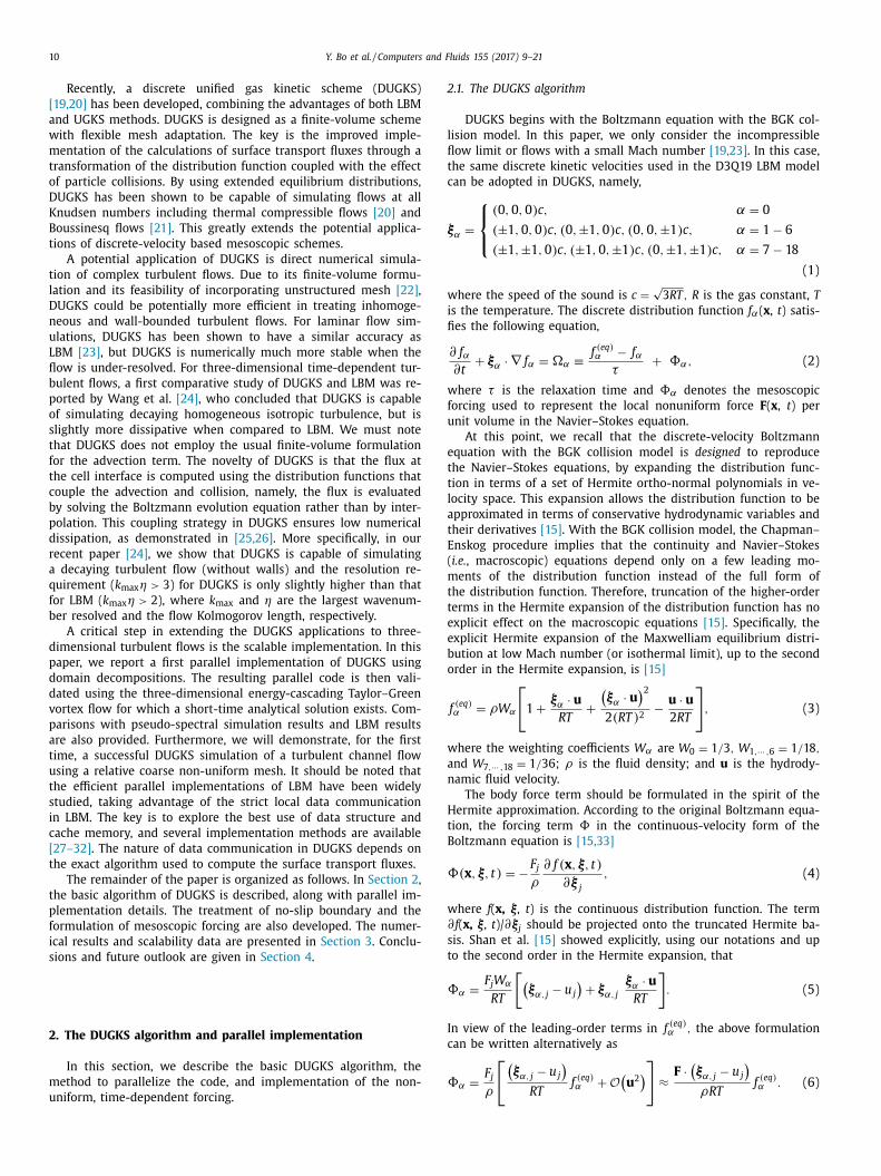
The parallel code makes use of two-dimensional domain de-
composition. Assume the physical domain is divided into nx × ny
× nz cells as shown in Fig. 1 . We divide the y direction into N py
parts and the z direction into N pz parts. A total of N p = N py N pz pro-
cessors are used, each handles a sub-domian of nx × ly × lz cells,
where ly = ny/N py and lz = nz/N pz . The main variable for each pro-
cessor is a four-dimensional ( i.e. , particle index and x, y, z loca-
tions) array ˜ f [f(0:np - 1,1:nx,1:ly,1:lz)], which is defined at the cell
centers, as shown in Fig. 1 , where np = 19 is the number of kinetic
particles.
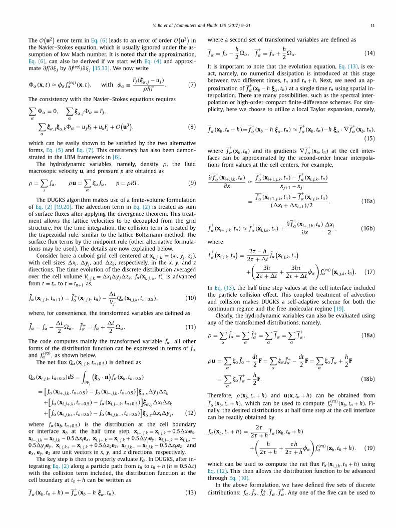
The algorithm is summarized using a block flow diagram in
Fig. 2 , where the large red box marks the main loop. There are 4
main subroutines: interface, flux, evolve, and macrovar. The inter-
face subroutine performs the following functions. First f +
[fb(0:np
- 1,0:nx+1,0:ly+1,0:lz+1)] is computed at the cell centers using Eq.
(17) . Here the hydrodynamic variables at ( x i, j, k , t n ) need to be
computed to obtain f ( eq ) ( x i, j, k , t n ) in Eq. (17) . Then it is extended to
include ghost cell centers as shown in Fig. 1 , by using the periodic
boundary condition, or for no-slip wall by extrapolation. For inte-
rior sub-domains, this extension requires data communication with
neighboring sub-domains. This extension is the only data com-
munication of the algorithm, which is handled by the MPI (Mes-
sage Passing Interface) library. Now the values of f + (x b , t n ) at the
cell interface nodes can be computed by interpolation from the
values at the cell centers and ghost cell centers. There are three
types of interface nodes: x −interface nodes, y −interface nodes, and
z−interface nodes; the values of f + (x , t n ) at these three types of
bnterface nodes are saved as fix(0:np - 1,0:lx,0:ly+1,0:lz+1), fiy(0:np
1,0:lx+1,0:ly,0:lz+1), and fiz(0:np - 1,0:lx+1,0:ly+1,0:lz).
The flux subroutine performs the computation of f α(x b , t n + h )
sing Eqs. (15) and (19) . Additional consideration for the no-slip
oundary condition will be explained in Section 2.3 . The val-
es of f α(x b , t n + h ) are saved in a temporary array fi(0:np -
,0:lx+1,0:ly+1,0:lz+1). Here the hydrodynamic variables at (x b , t n + ) need to be computed to obtain f (eq ) (x b , t n + h ) in Eq. (19) . This
rocess is repeated for the x, y , and z interface nodes. The same ar-
ays, fix, fiy, and fiz, can be used to store f α(x b , t n + h ) at the three
ypes of interface nodes.
The evolve subroutine performs the net flux calculation ac-
ording to Eq. (12) . At this point, ˜ f α(x i, j,k , t n + �t) can be read-
ly obtained by Eq. (10) . Finally, the hydrodynamic variables at
(x i, j,k , t n + �t) are obtained from
˜ f α(x i, j,k , t n + �t) in the macrovar
ubroutine.
The above description shows that only the interface subrou-
ine requires local sub-domain data communication. A total of five
arge arrays are used in the program, which consumes more mem-
ry than the LBM approach. The main advantage over LBM is that
UGKS allows the use of any non-uniform and anisotropic grid
tructure, as the grid structure is not coupled with the particle ve-
ocities. Two examples of using non-uniform grids will be provided
n Section 3.2 and Section 3.3 .
.3. Implementation of the no-slip boundary condition on the
hannel walls
Here we explain several other necessary details. First, for a solid
all boundary such as the channel walls inSecs. 3.2 and 3.3, the f +
alues at the ghost cell centers are determined by extrapolation,
imilar to the extrapolation method used in LBM in [35] . The no-
lip boundary condition is done using the concept of bounce-back.
owever, it is performed on the cell interfaces rather than along
attice links in LBM. This interface surface-based treatment has the
otential benefit of eliminating corner singularity, for example, for
he case of cavity flow simulations [23] . Consider a cell interface
hose outward normal is m , since in the examples we considered
n Section 3 , the walls are fixed. The general no-slip bounce-back
iscussed in [19] reduces simply to
f α(x b , t + h ) = f α(x b , t + h ) , for all ξα · m < 0 , (21)
hich should be executed after the reconstruction of f α( x , t n + h )n Eq. (13) , but before the transformation back to the original vari-
ble f α( x , t n + h ) , Eq. (19) . This order ensures a consistent compu-
ation of wall velocity needed for the transformation.
While we assumed a structured grid in the above discussions,
he finite-volume DUGKS formulation can be extended relatively
asily to unstructured grids, as has already been done in [22] .
. Results
In this section, we will perform three-dimensional flow simu-
ations using the parallel DUGKS code. We will compare the re-
ults from the pseudo-spectral method and the LBM method. For
eriodic flows, the pseudo-spectral method has been described in
42,43] , and for turbulent channel flow it is presented in [36,37] .
he LBM method follows the details provided in [38,39] .
.1. 3D Taylor-Green vortex flow with energy cascade
The 3D Taylor-Green vortex flow [40] is one of the very few
nalytical solutions of three-dimensional time-dependent Navier–
tokes equations. Starting from a simple incompressible 3D initial
ondition of the form
(x , t = 0) = cos (x ) sin (y ) sin (z) , (22a)
Y. Bo et al. / Computers and Fluids 155 (2017) 9–21 13
Fig. 1. A sketch showing the locations of cell-center nodes (filled circles) and related boundary nodes (diamonds for boundary nodes along the x direction, and squares for
boundary nodes along the y direction) and the ghost nodes (open circles). The grid spacing can be non-uniform in general. The distributions to be solved are defined only
at the cell-center nodes. The distributions at the ghost nodes are extended from the center-center nodes either by periodic boundary conditions or by extrapolation (for a
no-slip wall) from the cell-center nodes.
Fig. 2. Flow diagram of the parallel DUGKS code.
v
w
a
0
N
c
t
m
o
R
(x , t = 0) = − sin (x ) cos (y ) sin (z) , (22b)
(x , t = 0) = 0 , (22c)
nd assuming periodic conditions in a cubic domain: 0 ≤ x ≤ 2 π ,
≤ y ≤ 2 π , 0 ≤ z ≤ 2 π , the three-dimensional time-dependent
avier–Stokes equation
∂u
∂t + u · ∇u = − 1
ρ0
∇p +
1
R
∇
2 u (23)
an be solved analytically, at small times, using the short-time per-
urbation expansion. Here all quantities have been properly nor-
alized by the initial maximum velocity magnitude U 0 in the x
r y direction, and L B /2 π , where L B is the physical domain size,
= L U / (2 πν) is the flow Reynolds number divided by (2 π ), ν
B 0
14 Y. Bo et al. / Computers and Fluids 155 (2017) 9–21
Fig. 3. The resolution parameter k max η as a function of time, for different grid res-
olutions in the spectral simulation. The spectral truncation radius k max is set to
k max = N/ 3 by the 2/3 rule.
s
s
p
t
N
t
l
0
t
t
a
A
t
k
o
b
t
l
a
G
f
t
N
t
s
s
t
c
a
t
c
s
s
a
t
t
N
e
c
m
t
is the kinematic viscosity. The pressure p has been normalized by
ρU
2 0 .
Taylor and Green (TG37 hereafter) [40] obtained a perturbation
expansion of the velocity field, up to O(t 5 ) . Their solution for the
velocity field contains 8 distinct modes and is given as
u (x , t) = δ1 cos (x ) sin (y ) sin (z) + α1 sin (2 x ) cos (2 z)
+
2
3
γ2 cos (3 x ) sin (y ) sin (z)
+ γ2 cos (x ) sin (3 y ) sin (z)
−γ3 cos (x ) sin (y ) sin (3 z)
−β1 cos (3 x ) sin (y ) sin (3 z) , (24a)
v (x , t) = −δ1 sin (x ) cos (y ) sin (z) + α1 sin (2 y ) cos (2 z)
−γ2 sin (3 x ) cos (y ) sin (z)
−2
3
γ2 sin (x ) cos (3 y ) sin (z)
+ γ3 sin (x ) cos (y ) sin (3 z)
+ β1 sin (x ) cos (3 y ) sin (3 z) , (24b)
w (x , t) = −α1 [ cos (2 x ) + cos (2 y ) ] sin (2 z)
−γ2 sin (3 x ) sin (y ) cos (z)
+ γ2 sin (x ) sin (3 y ) cos (z)
+ β1 sin (3 x ) sin (y ) cos (3 z)
−β1 sin (x ) sin (3 y ) cos (3 z) , (24c)
where
δ1 =
[1 − 3 t
R
+
(9
R
2 − 1
16
)t 2
2
−(
27
2 R
2 − 23
32
)t 3
3 R
+
(31
132 · 64
− 185
48 R
2 +
27
2 R
4
)t 4
4
−(
555
44 · 32 · 8
− 2575
192 R
2 +
81
8 R
4
)t 5
5 R
], (25a)
α1 = −1
8
[t − 7 t 2
R
+
(74
3 R
2 − 43
44 · 12
)t 3 −
(175
3 R
3 − 43
44
)t 4
4
],
(25b)
β1 (x , t = 0) = − 1
16
t 2 (
1
2
− 13
2
t
R
), (25c)
γ2 (x , t = 0) = − 15
176
t 2 (
1
2
− 31
6
t
R
), (25d)
γ3 (x , t = 0) = − 1
16
t 2 (
1
2
− 31
6
t
R
). (25e)
Clearly, as smaller scale fluid motion is generated over time,
and the process of energy transfer from large to small scales was
the original motivation for TG37. Based on this perturbation solu-
tion, TG37 provided prediction of the flow kinetic energy and dis-
sipation rate at short times. Note that this energy transfer across
scales is not present in the 2D Taylor-Green vortex flow often used
to benchmark numerical methods in two spatial dimensions [41] .
The parameter settings for our simulation are shown in Table 1 .
All the simulations are set with the physical Reynolds number
Re = U 0 L B /ν = 600 π . The velocity scale in LBM is chosen such that,
at the same grid resolution N , one LBM time step is equivalent
to one spectral time step. The LBM MRT parameters are [39] :
9 = d t/ (3 ν + 0 . 5 d t) , s 1 = 1 . 19 , s 2 = 1 . 4 , s 4 = 1 . 2 , s 10 = 1 . 4 , s 13 = 9 , s 16 = 1 . 98 , ω ε = 0 . 0 , ω ε j = −475 / 63 , and ω xx = 0 . 0 .
For the spectral simulation, as shown in Fig. 3 , the resolution
arameter k max η changes from 0.662, 0.965, 1.935, 3.871 at ˜ t = 0
o 0.494, 1.32, 2.65, 5.29 at ˜ t = 10 , for the different grid resolutions
= 32 , 64 , 128 , 256 , respectively, where k max = N/ 3 is the spectral
runcation radius in the spectral code and η is the Kolmogorov
ength. The minimum k max η occurs around
˜ t = 6 . 2 and is 0.437,
.897, 1.79, 3.59, for N = 32 , 64 , 128 , 256 , respectively ( Fig. 3 ). Here
he dimensionless time is defined as ˜ t = 2 πU 0 t/L B . This indicates
he flow is not resolved at N = 32 , barely resolved at N = 64 ,
nd well resolved at N = 128 , 256 in the spectral simulation [42] .
s confirmed below, the results from N = 64 and N = 128 spec-
ral simulations are almost identical. Note that the requirement of
max η > 1 for a well-resolved spectral simulation [42] was devel-
ped based on fully-developed forced homogeneous isotropic tur-
ulence, and should only be taken as a reference. For example,
he initial flow here is not a turbulent flow and contains only the
arge-scale, so the k max η parameter is not meaningful.
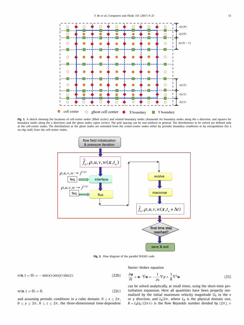
The time evolutions of the kinetic energy and dissipation rate
re shown in Fig. 4 . Four groups of results are shown: the Taylor–
reen short-time theoretical results [40] , and numerical results
rom three different codes: spectral, LBM, and DUGKS. The spec-
ral results at N = 128 can be viewed as the benchmark for others.
ote that the spectral results at N = 256 (not shown) are essen-
ially identical to the spectral results at N = 128 . A number of ob-
ervations can be made. First, all results are identical for ˜ t < 2 . 0 ,
howing that the theoretical short-time expansion is accurate for˜ < 2 . 0 as long as the kinetic energy and dissipation rate are con-
erned. Also all codes at the two resolutions ( N = 64 , 128 ) shown
dequately resolve the flow for ˜ t < 2 . 0 , since at the early times
he flow is dominated by large-scale initial flow, and the energy-
ascading process has not yet generated the motion at the smallest
cales. Second, the flow appears to be adequately resolved by the
pectral code even at N = 64 as the results from the spectral code
t N = 64 are essentially identical to those at N = 128 , for both
he kinetic energy and the dissipation rate, at all times shown in
he plots. This confirms that the results from the spectral code at
= 128 and above can be used as the benchmark. The kinetic en-
rgy decays monotonically. However, the dissipation rate first in-
reases due to production of small-scale flow structures, reaches a
aximum at ˜ t ≈ 6 , and then decreases again due to reduction of
he overall flow Reynolds number. Third, LBM and DUGKS results
Y. Bo et al. / Computers and Fluids 155 (2017) 9–21 15
Table 1
Parameter settings for the 3D Taylor–Green vortex flow.
Label N U 0 L B ν R ≡ U 0 L B 2 πν dt U 0 dt / dx K (0) D (0)
Spectral 32/64/128/256 1 .0 2 π 1 300
300 0 . 64 N
0 .1018591 0 .125 0 .0025
LBM 32/64/128 0 .1018591 N U 0 N 600 π 300 1 .0 0 .1018591 0.125 U 2 0 0 . 0025 · 2 πU 3 0
L B
DUGKS 32/64/128 0 .1018591 N U 0 N 600 π 300 0 .5 0 . 1018591
2 0.125 U 2 0 0 . 0025 · 2 πU 3 0
L B
a b
Fig. 4. (a) Kinetic energy and (b) dissipation rate as a function of time, for the 3D Taylor–Green vortex flow at Re = 300 . All quantities are normalized as indicated.
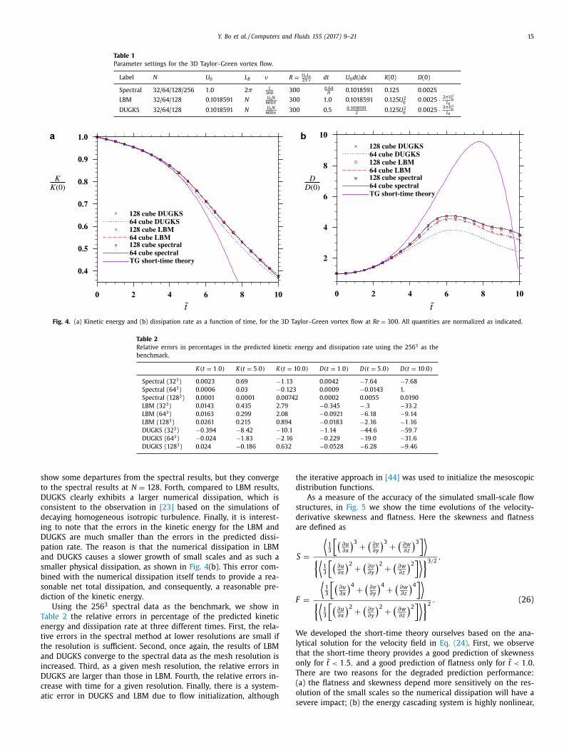
Table 2
Relative errors in percentages in the predicted kinetic energy and dissipation rate using the 256 3 as the
benchmark.
K(t = 1 . 0) K(t = 5 . 0) K(t = 10 . 0) D (t = 1 . 0) D (t = 5 . 0) D (t = 10 . 0)
Spectral (32 3 ) 0 .0023 0 .69 −1 . 13 0 .0042 −7 . 64 −7 . 68
Spectral (64 3 ) 0 .0 0 06 0 .03 −0 . 123 0 .0 0 09 −0 . 0143 1.
Spectral (128 3 ) 0 .0 0 01 0 .0 0 01 0 .00742 0 .0 0 02 0 .0055 0 .0190
LBM (32 3 ) 0 .0143 0 .435 2 .79 −0 . 345 −. 3 −33 . 2
LBM (64 3 ) 0 .0163 0 .299 2 .08 −0 . 0921 −6 . 18 −9 . 14
LBM (128 3 ) 0 .0261 0 .215 0 .894 −0 . 0183 −2 . 16 −1 . 16
DUGKS (32 3 ) −0 . 394 −8 . 42 −10 . 1 −1 . 14 −44 . 6 −59 . 7
DUGKS (64 3 ) −0 . 024 −1 . 83 −2 . 16 −0 . 229 −19 . 0 −31 . 6
DUGKS (128 3 ) 0 .024 −0 . 186 0 .632 −0 . 0528 −6 . 28 −9 . 46
s
t
D
c
d
i
D
p
a
s
b
s
d
T
e
t
t
a
i
D
c
a
t
d
s
d
a
F
W
l
t
o
T
(
o
how some departures from the spectral results, but they converge
o the spectral results at N = 128 . Forth, compared to LBM results,
UGKS clearly exhibits a larger numerical dissipation, which is
onsistent to the observation in [23] based on the simulations of
ecaying homogeneous isotropic turbulence. Finally, it is interest-
ng to note that the errors in the kinetic energy for the LBM and
UGKS are much smaller than the errors in the predicted dissi-
ation rate. The reason is that the numerical dissipation in LBM
nd DUGKS causes a slower growth of small scales and as such a
maller physical dissipation, as shown in Fig. 4 (b). This error com-
ined with the numerical dissipation itself tends to provide a rea-
onable net total dissipation, and consequently, a reasonable pre-
iction of the kinetic energy.
Using the 256 3 spectral data as the benchmark, we show in
able 2 the relative errors in percentage of the predicted kinetic
nergy and dissipation rate at three different times. First, the rela-
ive errors in the spectral method at lower resolutions are small if
he resolution is sufficient. Second, once again, the results of LBM
nd DUGKS converge to the spectral data as the mesh resolution is
ncreased. Third, as a given mesh resolution, the relative errors in
UGKS are larger than those in LBM. Fourth, the relative errors in-
rease with time for a given resolution. Finally, there is a system-
tic error in DUGKS and LBM due to flow initialization, although
she iterative approach in [44] was used to initialize the mesoscopic
istribution functions.
As a measure of the accuracy of the simulated small-scale flow
tructures, in Fig. 5 we show the time evolutions of the velocity-
erivative skewness and flatness. Here the skewness and flatness
re defined as
S =
⟨ 1 3
[ (∂u ∂x
)3 +
(∂v ∂y
)3 +
(∂w
∂z
)3 ] ⟩
{ ⟨ 1 3
[ (∂u ∂x
)2 +
(∂v ∂y
)2 +
(∂w
∂z
)2 ] ⟩ } 3 / 2
,
=
⟨ 1 3
[ (∂u ∂x
)4 +
(∂v ∂y
)4 +
(∂w
∂z
)4 ] ⟩
{ ⟨ 1 3
[ (∂u ∂x
)2 +
(∂v ∂y
)2 +
(∂w
∂z
)2 ] ⟩ } 2
. (26)
e developed the short-time theory ourselves based on the ana-
ytical solution for the velocity field in Eq. (24) . First, we observe
hat the short-time theory provides a good prediction of skewness
nly for ˜ t < 1 . 5 , and a good prediction of flatness only for ˜ t < 1 . 0 .
here are two reasons for the degraded prediction performance:
a) the flatness and skewness depend more sensitively on the res-
lution of the small scales so the numerical dissipation will have a
evere impact; (b) the energy cascading system is highly nonlinear,
16 Y. Bo et al. / Computers and Fluids 155 (2017) 9–21
a b
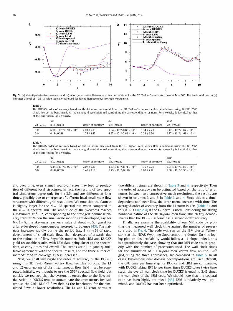
Fig. 5. (a) Velocity-derivative skewness and (b) velocity-derivative flatness as a function of time, for the 3D Taylor–Green vortex flow at Re = 300 . The horizontal line on (a)
indicates a level of −0 . 5 , a value typically observed for forced homogeneous isotropic turbulence.
Table 3
The DUGKS order of accuracy based on the L1 norm, measured from the 3D Taylor–Green vortex flow simulations using DUGKS 256 3
simulation as the benchmark. At the same grid resolution and same time, the corresponding error norm for v velocity is identical to that
of the error norm for u velocity.
32 3 64 3 128 3
2 πU 0 t / L B u ( L 1)/ w ( L 1) Order of accuracy u ( L 1)/ w ( L 1) Order of accuracy u ( L 1)/ w ( L 1)
1 .0 6 . 98 × 10 −3 / 3 . 93 × 10 −2 2 .09 / 2.16 1 . 64 × 10 −3 / 8 . 80 × 10 −3 1 .34 / 2.23 6 . 47 × 10 −4 / 1 . 87 × 10 −3
5 .0 0 .154/0.211 1 .75 / 1.47 4 . 57 × 10 −2 / 7 . 62 × 10 −2 2 .23 / 2.24 9 . 77 × 10 −3 / 1 . 63 × 10 −2
Table 4
The DUGKS order of accuracy based on the L2 norm, measured from the 3D Taylor-Green vortex flow simulations using DUGKS 256 3
simulation as the benchmark. At the same grid resolution and same time, the corresponding error norm for v velocity is identical to that
of the error norm for u velocity.
32 3 64 3 128 3
2 πU 0 t / L B u ( L 2)/ w ( L 2) Order of accuracy u ( L 2)/ w ( L 2) Order of accuracy u ( L 2)/ w ( L 2)
1 .0 6 . 44 × 10 −3 / 3 . 90 × 10 −2 2 .07 / 2.16 1 . 53 × 10 −3 / 8 . 71 × 10 −3 1 .35 / 2.24 6 . 01 × 10 −4 / 1 . 85 × 10 −3
5 .0 0 .182/0.286 1 .49 / 1.18 6 . 49 × 10 −2 / 0 . 126 2 .02 / 2.12 1 . 60 × 10 −2 / 2 . 90 × 10 −2
t
t
n
s
d
a
t
n
s
t
s
s
l
i
e
f
g
c
t
w
s
t
c
m
and over time, even a small round-off error may lead to produc-
tion of different local structures. In fact, the results of two spec-
tral simulations agree only for ˜ t < 3 . 5 , and are different at later
times, possibly due to emergence of different local small-scale flow
structures with different grid resolutions. We note that the flatness
is slightly larger for the N = 128 spectral run when compared to
the N = 64 spectral run. The amplitude of the skewness reaches
a maximum at ˜ t = 2 , corresponding to the strongest nonlinear en-
ergy transfer. When the small-scale motions are developed, say, for
6 < ̃
t < 8 , the skewness reaches a value of about −0 . 5 , typical for
a fully-developed homogeneous isotropic turbulence [43] . The flat-
ness increases rapidly during the period ( i.e. , 3 < ̃
t < 5 ) of rapid
development of small-scale flow, then decreases afterwards due
to the reduction of flow Reynolds number. Both LBM and DUGKS
yield reasonable results, with LBM data being closer to the spectral
data, at early times and overall. The trends are all in good quanti-
tative agreement with the spectral results, and the three numerical
methods tend to converge as N is increased.
Next, we shall investigate the order of accuracy of the DUGKS
using this 3D Taylor-Green vortex flow. For this purpose, the L1
and L2 error norms of the instantaneous flow field must be com-
puted. Initially, we thought to use the 256 3 spectral flow field, but
quickly we realized that the systematic errors due to the flow ini-
tialization in DUGKS tend to contaminate the error norms. Instead,
we use the 256 3 DUGKS flow field as the benchmark for the sim-
ulated flows at lower resolutions. The L1 and L2 error norms at
wo different times are shown in Table 3 and 4 , respectively. Then
he order of accuracy can be estimated based on the ratio of error
orms between two consecutive mesh resolutions, the results are
hown in columns 3 and 5 in Table 3 and 4 . Since this is a time-
ependent nonlinear flow, the error norms increase with time. The
veraged order of accuracy from the L1 norm is 1.94 ( Table 3 ), and
his is 1.83 ( Table 4 ) if the L2 norm is used. Considering the strong
onlinear nature of the 3D Taylor-Green flow, This clearly demon-
trates that the DUGKS scheme has a second-order accuracy.
Finally, we examine the scalability of our MPI code by plot-
ing the measured wall clock time against the number of proces-
ors used in Fig. 6 . The code was run on the IBM cluster Yellow-
tone at the NCAR-Wyoming Supercomputing Center. On this log-
og plot, an ideal scalability would follow a −1 slope. Indeed, this
s approximately the case, showing that our MPI code scales prop-
rly with the number of processors used. The wall clock times
or the simulation of 3D Taylor-Green vortex flow on the 128 3
rid, using the three approaches, are compared in Table 5 . In all
ases, two-dimensional domain decompositions are used. Overall,
he CPU time per time step for DUGKS and LBM are comparable,
ith DUGKS taking 19% longer time. Since DUGKS takes twice time
teps, the overall wall clock time for DUGKS is equal to 2.43 times
he wall clock of the LBM code. We should note that the spectral
ode has been highly optimized [45] , LBM is relatively well opti-
ized, and DUGKS has not been optimized.

Y. Bo et al. / Computers and Fluids 155 (2017) 9–21 17
Table 5
Comparison of wall clock times with 16 processors, for simulations of 3D Taylor–Green vortex flow on the 128 3 grid for a time period of
2 πU 0 t/L B = 10 . 0 .
2 πU 0 dt / L B total time steps Total CPU time (s) Wall clock time per step (s) Ratio / time step Overall Ratio
Spectral 0 .005 10 0 0 2969 0 .185 1 1
LBM 0 .005 10 0 0 12,519 0 .782 4 .2 4 .2
DUGKS 0 .0025 20 0 0 30,052 0 .939 5 .1 10 .2
Table 6
Parameter settings for the laminar channel flow simulations.
Label N 1 × N 2 × N 3 u max r G d x min /d x max 2 H ν Re ≡ 2 u max H ν dt
√
6 · c s d t/d x min
Case 1 40 × 4 × 4 0 .1 0 .0 1 .0 30 .4891 0 .2186 18 .3 0 .35355 0 .5
Case 2 40 × 4 × 4 0 .1 3 .0 0 .1938 24 .1825 0 .1322 18 .3 0 .077182 0 .5632
Fig. 6. Measured wall clock time as a function of the number of processors used.
The line shows a power law of −1 slope.
3
S
l
a
b
x
w
u
N
s
T
t
c
H
T
m
t
s
w
t
o
t
c
o
a
a
n
p
c
a
u
f
3
l
m
t
a
t
m
d
i
s
L
w
t
c
b
i
T
a
p
c
t
fi
fi
r
D
.2. The laminar channel flow
Before reporting the results for a turbulent channel flow in
ection 3.3 , we demonstrate briefly the simulation of transient
aminar channel flow, as in this case the flow can be solved an-
lytically.
A non-uniform mesh in the wall-normal direction is defined the
y locations of the cell faces as
f (i )=
tanh (0 . 5 r G ) + tanh
[r G
( i −N 1 / 2−1 ) N 1
]tanh
(r G N 1
) , for i = 1 , 2 , . . . , N 1 + 1 ,
(27)
here r G is a parameter used to adjust the degree of non-
niformity. This defines a symmetric mesh with respect to i = 1 / 2 + 1 . The mesh is defined such that the maximum mesh
ize is one unit, namely, dx max = x f (N 1 / 2 + 1) − x f (N 1 / 2) = 1 .
he minimum mesh size is dx min = x f (2) − x f (1) = [ tanh (0 . 5 r G ) +anh (r G /N 1 − 0 . 5 r G )] / tanh (r G /N 1 ) . The above mesh specifies the
hannel half-width as
=
tanh (0 . 5 r G )
tanh
(r G N 1
) . (28)
he limiting case of r G → 0 represents the uniform mesh. Two
eshes with r G = 0 and r G = 3 are considered ( Table 6 ). N 1 is set
o 40. Since there is no dependence on y and z, N 2 and N 3 can be
et to any value.
The analytical solution of the laminar transient flow is
v (x, t)
v max = F ( x n , t n ) =
(1 − x 2 n
)−
∞ ∑
k =0
(−1) k · 4
[(k + 0 . 5) π ] 3
× cos [ (k + 0 . 5) πx n ] exp
[−(k + 0 . 5) 2 π2 t n
], (29)
here x n = x/H and t n ≡ νt / H
2 .
Fig. 7 shows the simulated velocity profiles at five different
imes with both the uniform grid and non-uniform grid. The the-
retical solutions are also shown. The theoretical solutions are ob-
ained using 300 terms in the summation in Eq. (29) . Clearly, in all
ases, the DUGKS results are in excellent agreement with the the-
retical solutions. The difference between the simulated velocity
nd the theoretical value is plotted in Fig. 8 . In both cases, there
ppears to be a positive fixed error at the wall for the specific
o-slip boundary treatment we used. The errors inside are mostly
ositive, except at early times that they may be negative near the
hannel center. The shape and magnitude of the error profiles are
ffected by the mesh structure, but overall the errors for the non-
niform mesh case (Case 2) are comparable to those for the uni-
orm mesh case (Case 1).
.3. The turbulent channel flow
The parameter settings for the turbulent channel flow simu-
ation are shown in Table 7 . Specifically, the same nonuniform
esh defined by Eq. (27) is used in the wall normal (x) direc-
ion, with N 1 = 128 and r G = 4 . 0 . This setting yields dx min = 0 . 0728
nd a channel half width of H = 30 . 8589 . A 128 3 mesh resolu-
ion is used. The DUGKS domain size matches the spectral do-
ain size, therefore, dy = 3 . 03 , and dz = 1 . 01 . The CFL number is
t √
2 /d x min = 0 . 90 . In terms of the wall unit, dx + min
= 0 . 425 , which
s sufficient to resolve the wall layer [46] . With the parameters
hown in Table 7 , roughly 6 DUGKS time steps correspond to one
BM time step.
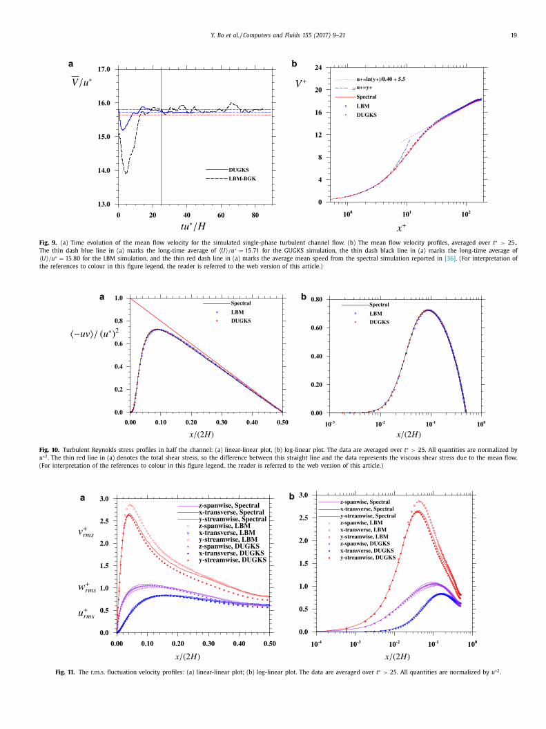
In Fig. 9 (a), we show the mean flow speed (averaged over the
hole flow domain) as a function of non-dimensional time t ∗ ≡u ∗/ H . A nonuniform force field described in [39] was added to the
onstant physical driving force, to excite the development of tur-
ulent flow during 0 < t ∗ < 0.526. The same perturbation forc-
ng with identical parameters was applied in the LBM simulation.
he difference in the mean flow speed at t ∗ = 0 between DUGKS
nd LBM was due to the use of slightly different initial mean flow
rofiles in the two simulations. Initially, the mean flow speed de-
reases as the kinetic energy is transferred from the mean flow to
he turbulent fluctuations. After t ∗ = 0 . 526 , the nonuniform force
eld is removed, and the mean flow speed continues to evolve,
rst reaches a minimum mean flow speed at around t ∗ = 4 . 5 , then
ebounds and gradually reaches a stationary value. For both the
UGKS and LBM runs, the flow appears to be stationary at around

18 Y. Bo et al. / Computers and Fluids 155 (2017) 9–21
a b
Fig. 7. Velocity profiles for the transient laminar flow: (a) uniform grid with 2 H = 40 . 0 , and (b) nonuniform grid with 2 H = 24 . 1825 . The symbols are the simulated DUGKS
data and the lines are the theoretical solutions. Re = 18 . 3 .
a b
Fig. 8. The relative errors for the DUGKS transient laminar flow: (a) uniform grid with 2 H = 40 . 0 , and (b) nonuniform grid with 2 H = 24 . 1825 .
Table 7
Parameter settings for the turbulent channel flow simulations.
Run N 1 × N 2 × N 3 Domain size H ν u ∗ Re τ δx min / ( ν/u ∗) ( < 2.25 [46] ) u ∗2 dt / ν
Spectral [36] 129 × 192 × 160 2 H × 4 πH × 4 πH /3 - - - 180 0 .054 -
LBM [39] 200 × 400 × 200 2 H × 4 H × 2 H 100 0 .0036 0 .00648 180 1 .806 0 .01166
DUGKS 128 × 128 × 128 2 H × 4 πH × 4 πH /3 30 .86 0 .0012 0 .007 180 0 .425 0 .001893
m
i
a
T
y
i
s
b
i
v
a
D
a
t
I
a
u ∗t/H = 25 . The average mean speed averaged for u ∗t / H > 25 is
15.71 from the DUGKS simulation and 15.80 for the LBM simu-
lation, and relative difference is about 0.6%. Due to the use of a
much large computational domain size in DUGKS, the variations of
the mean flow speed with time in DUGKS are much smaller than
those in LBM. As a comparison, the mean flow speed in the spec-
tral simulation reported in [36] at the same flow Reynolds number
was 15.63. Therefore, the DUGKS mean flow speed is 0.5% larger
than the spectral benchmark, while the LBM mean flow speed is
1.1% larger than the spectral benchmark, implying that the DUGKS
yields a better result in terms of the mean flow speed. The rela-
tive error in DUGKS is due only to the numerical truncation error,
while the relative error in LBM is due to both the domain size ef-
fect and numerical truncation error.
Next, we show profiles averaged over time after t ∗ = 25 .
Fig. 9 (b) displays the mean velocity profiles on a log-linear plot.
Here, the legend “Spectral” refers to the data from the Chebychev-
spectral simulation done by the Stanford group [36,37] using a do-
ain size 4 πH × 2 H × 4 πH /3. In wall units, the channel center
s at x + = 180 . The DUGKS result is very close to the LBM result,
nd both are in reasonable agreement with the spectral results.
he profile fits well the standard linear viscous sublayer scaling for
+ < 5 , and the inertial sublayer scaling starting at y + > 30 . In the
nertial sublayer, the mean velocity from the DUGKS and LBM is
lightly larger than the spectral benchmark data.
The averaged Reynolds stress profiles are shown in Fig. 10 , in
oth linear-linear and log-linear plots. The center of the channel
s at x/ (2 H) = 0 . 5 . The sum of Reynolds stress and viscous stress
aries linearly from the channel center to the channel wall. All data
re in good agreement. When compared to the spectral result, the
UGKS result is clearly better than the LBM result in the near wall
nd buffer regions ( x /(2 H ) < 0.15).
Finally, the rms velocity profiles are shown in Fig. 11 . Overall,
he profiles from the DUGKS and LBM are in reasonable agreement.
n the near-wall regions, the streamwise rms velocity is the largest
nd the transverse rms velocity is the smallest. The DUGKS results
Y. Bo et al. / Computers and Fluids 155 (2017) 9–21 19
a b
Fig. 9. (a) Time evolution of the mean flow velocity for the simulated single-phase turbulent channel flow. (b) The mean flow velocity profiles, averaged over t ∗ > 25..
The thin dash blue line in (a) marks the long-time average of 〈 U〉 /u ∗ = 15 . 71 for the GUGKS simulation, the thin dash black line in (a) marks the long-time average of
〈 U〉 /u ∗ = 15 . 80 for the LBM simulation, and the thin red dash line in (a) marks the average mean speed from the spectral simulation reported in [36] . (For interpretation of
the references to colour in this figure legend, the reader is referred to the web version of this article.)
a b
Fig. 10. Turbulent Reynolds stress profiles in half the channel: (a) linear-linear plot, (b) log-linear plot. The data are averaged over t ∗ > 25. All quantities are normalized by
u ∗2 . The thin red line in (a) denotes the total shear stress, so the difference between this straight line and the data represents the viscous shear stress due to the mean flow.
(For interpretation of the references to colour in this figure legend, the reader is referred to the web version of this article.)
a b
Fig. 11. The r.m.s. fluctuation velocity profiles: (a) linear-linear plot; (b) log-linear plot. The data are averaged over t ∗ > 25. All quantities are normalized by u ∗2 .

20 Y. Bo et al. / Computers and Fluids 155 (2017) 9–21
s
T
2
o
w
g
e
r
i
s
s
o
4
D
s
w
a
L
s
c
a
c
s
m
t
s
s
p
l
t
n
d
a
D
m
D
p
f
A
F
A
g
M
e
s
U
h
d
N
a
0
R
for the streamwise and spanwise rms velocities in the near-wall
region ( x /(2 H ) < 0.15) are better than the LBM results when com-
pared to the spectral benchmark. In the center region of the chan-
nel, the DUGKS result in the streamwise direction appears to devi-
ate more from the spectral data for two reasons. First, the DUGKS
resolution is perhaps too coarse in the channel center region in
both transverse and streamwise directions and the numerical dis-
sipation is significant. Second, the LBM result at the peak location
overshoots due to the domain size effect [39] ; this combined with
the numerical dissipation in LBM makes the results appear better
in the center region. Overall, we may still claim that the DUGKS
results are better given the coarser resolution used in DUGKS (see
Table 7 ) to cover a larger domain. Different distribution of grid
points in the transverse direction and different grid resolutions
should be tested, which could be a topic for future work.
We note that the numerical dissipation in DUGKS depends on
the time step size (or the CFL number), as shown in Zhu et al. [34] .
A smaller time step implies a smaller numerical dissipation and
more accurate solution. Since in our turbulent channel flow simu-
lation, the time step size is derived from the CFL number based on
the smallest lattice spacing near the channel wall, the time step is
indeed very small, which could be the reason for accurate turbu-
lence statistics from DUGKS.
In summary, the first simulation of turbulent channel flow us-
ing DUGKS shows that the results are reasonably accurate. Of sig-
nificance is that these preliminary DUGKS results are obtained
with a coarse grid resolution covering a large domain size, thus
the grid cell aspect ratios near the wall are large. The maximum
aspect ratio measured in terms of streamwise lattice spacing to
transverse lattice spacing near the wall is 41.62. Since the standard
LBM uses a cubic lattice, it is costly to cover the same domain size,
so a smaller domain size was used here. Recently, we have shown
that it is possible to extend the D3Q19 LBM to a cuboid grid [47] ,
but the cuboid model could have numerical stability issues at large
aspect ratios. The DUGKS code is numerically stable for grid cells
with large aspect ratios.
4. Summary and outlook
In this paper, we report on parallel implementation of the re-
cently developed mesoscopic DUGKS scheme [19,20] for simulat-
ing three-dimensional flows. When dealing with incompressible
flows, the same D3Q19 lattice velocity model used in LBM can
be adopted. However, the transport term is treated as the sum of
fluxes across the interfaces of a grid cell volume. This removes
the restriction on the grid structure of the standard LBM, mak-
ing it feasible to incorporate non-uniform and irregular grids. The
treatment of the transport term is more involved compared to
the streaming operation in LBM, but the transformation from the
linkwise streaming in LBM to surface fluxes in DUGKS has po-
tential benefits of removing corner singularity and generating a
much more stable scheme. In this paper, we consider only non-
uniform structured grids, and the parallel implementation is rela-
tively straightforward. Besides the details of DUGKS algorithm im-
plementation, we have also documented the implementations of
a non-uniform grid, no-slip wall and non-uniform time-dependent
forcing. The MPI code based on two-dimensional domain decom-
position shows a good scalability.
The resulting parallel code was first tested for the 3D scale-
evolving Taylor–Green vortex flow, and DUGKS results are com-
pared to the Taylor-Green short-time analytical solution [40] and
numerical results from pseudo-spectral method and LBM. The ac-
curacy of the Taylor–Green short-time analytical solution can be
accessed by the high-resolution spectral solution. It was found that
DUGKS can provide accurate results with adequate grid resolu-
tion. The numerical errors in DUGKS are larger than those in LBM,
howing that DUGKS is more dissipative when compared to LBM.
his is consistent with the conclusion in [24] . Using the DUGKS
56 3 flow as the benchmark, we have demonstrated the second-
rder accuracy of the DUGKS scheme.
DUGKS results for a transient laminar channel flow agree well
ith the theoretical solution, with both uniform and non-uniform
rids in the wall-normal direction. Here we only considered the
xtrapolated bounced back for the no-slip wall. The numerical er-
or on the wall is related to how the distribution on the boundary
s constructed, which needs further investigation.
A first DUGKS simulation of the turbulent channel flow was
uccessfully performed, and results were compared to LBM and
pectral results. We find that even with the use of a cuboid grid
f very large aspect ratio (in our case the largest aspect ratio is
1.62 near the wall), the DUGKS code is numerically stable. The
UGKS results are better than the LBM results, in terms of the
imulated mean flow speed and turbulence statistics in the near
all and buffer regions. This is very encouraging given that a rel-
tively coarse grid was used for a large computational domain.
BM with a uniform cubic grid could not handle the same domain
ize with limited computational resources [39] . Furthermore, a 3D
uboid LBM model has recently been developed, but even at grid
spect ratio of 2.0, the cuboid LBM code was found to be numeri-
ally unstable [47] . Although the time step size in DUGKS has to be
mall due to the use of non-uniform grid, but the reduced grid size
akes the overall computational cost of DUGKS to be comparable
o LBM. This combined with our recent work on using DUGKS to
imulate decaying homogeneous isotropic turbulence [24] clearly
hows that DUGKS can be used as a DNS tool for turbulent flows,
articularly compressible and thermal turbulent flows. Neverthe-
ess the work here is considered preliminary, further examples of
urbulent flow simulations using DUGKS at higher flow Reynolds
umbers and different flow configurations are needed to further
ocument the capabilities and accuracy of DUGKS relative to LBM
nd other methods. While in this paper, DUGKS was used as a
NS tool since the local grid spacings in all spatial directions were
ade sufficiently small, to adequately resolve all scales of the flow.
ue to its nature as a finite-volume formulation, DUGKS has the
otential to be used as an implicit large-eddy simulation (LES) tool
or high-Reynolds number flows at a given grid resolution.
cknowledgements
This work has been supported by the U.S. National Science
oundation (NSF) under grants CNS1513031, CBET-1235974, and
GS-1139743 and by Air Force Office of Scientific Research under
rant FA9550-13-1-0213. LPW also acknowledges support from the
inistry of Education of P.R. China and Huazhong University of Sci-
nce and Technology through Chang Jiang Scholar Visiting Profes-
orship. LPW would like to acknowledge the travel support from
.S. National Science Foundation (NSF) to attend ICMMES-2015,
eld in CSRC ( www.csrc.ac.cn ), Beijing, July 20, – 24, 2015, un-
er the Grant CBET-1549614. Computing resources are provided by
ational Center for Atmospheric Research through CISL-P35751014,
nd CISL-UDEL0 0 01 and by University of Delaware through NSF CRI
958512.
eferences
[1] Eggels JG . Direct and large-eddy simulation of turbulent fluid flow using thelattice Boltzmann scheme. Int J Heat Fluid Flow 1996;17(3):307–23 .
[2] Chen S , Doolen G . Lattice Boltzmann method for fluid flows. Annu. Rev. FluidMech. 1998;30:329–64 .
[3] Yu D , Mei R , Luo L-S , Shyy W . Viscous flow computations with the method of
lattice Boltzmann equation. Prog Aerosp Sci. 2003;39:329–67 . [4] Chen H , Kandasamy S , Orszag S , Shock R , Succi S , Yakhot V . Extended Boltz-
mann kinetic equation for turbulent flows. Science 2003;301(5633):633–6 . [5] Yu H , Luo L-S , Girimaji SS . LES Of turbulent square jet flow using an MRT lat-
tice Boltzmann model. Comput Fluids 2006;35(8):957–65 .
Y. Bo et al. / Computers and Fluids 155 (2017) 9–21 21
[
[
[
[
[
[
[
[
[
[
[
[
[
[
[
[
[
[
[
[6] Guo Z , Shu C . Lattice boltzmann method and its applications in engineering(advances in computational fluid dynamics). World Scientific Publishing Com-
pany; 2013 . [7] Wang L-P, Peng C, Guo ZL, Yu ZS. Flow modulation by finite-size neu-
trally buoyant particles in a turbulent channel flow. ASME J Fluids Engr2016a;138:041103. doi: 10.1115/1.4031691 .
[8] Marié S , Ricot D , Sagaut P . Comparison between lattice Boltzmann method andNavier–Stokes high order schemes for computational aeroacoustics. J Comp
Phys 2009;228:1056–70 .
[9] Peng Y , Liao W , Luo L-S , Wang L-P . Comparison of the lattice Boltzmann andpseudo-spectral methods for decaying turbulence: low-order statistics. Comput
Fluids 2010;39(4):568–91 . [10] Gao H , Li H , Wang L-P . Lattice Boltzmann simulation of turbulent flow laden
with finite-size particles. Comput Math Appl 2013;65(2):194–210 . [11] Wang L-P , Ayala O , Gao H . Study of forced turbulence and its modulation by
finite-size solid particles using the lattice Boltzmann approach. Comp Math
Appl 2014;67:363–80 . [12] Guo ZL , Zhao TS , Shi Y . Physical symmetry, spatial accuracy, and relax-
ation time of the lattice boltzmann equation for microgas flows. J Appl Phys2006;99:074903 .
[13] Zhang YH , Gu XJ , Barber RW , Emerson DR . Capturing Knudsen layer phenom-ena using a lattice Boltzmann model. Phys Rev E 2006;74:046704 .
[14] Guo ZL , Zheng CG , Shi BC . Lattice Boltzmann equation with multiple effective
relaxation times for gaseous microscale flow. Phys Rev E 2008;77:036707 . [15] Shan X , Yuan XF , Chen H . Kinetic theory representation of hydrodynamics: a
way beyond the Navier-Stokes equation. J Fluid Mech 2006;550:413–41 . [16] Xu K , Huang JC . A unified gas-kinetic scheme for continuum and rarefied flows.
J Comput Phys 2010;229:7747–64 . [17] Xu K . Direct modeling for computational fluid dynamics: construction and ap-
plication of unified gas-kinetic schemes. World Scientific, Singapore; 2015a .
[18] Xu K . Direct modeling for computational fluid dynamics. Acta Mech Sin2015b;31:303–18 .
[19] Guo Z , Xu K , Wang R . Discrete unified gas kinetic scheme for all knudsen num-ber flows: low-speed isothermal case. Phys Rev E 2013;88(3):033305 .
20] Guo Z , Wang R , Xu K . Discrete unified gas kinetic scheme for all Knudsen num-ber flows. II Thermal compressible case. Phys Rev E 2015;91(3):033313 .
[21] Wang P , Wang L-P , Guo Z . A coupled discrete unified gas-kinetic scheme for
Boussinesq flows. Comput Fluids 2015a;120:70–81 . 22] Zhu L , Guo Z , Xu K . Discrete unified gas kinetic scheme on unstructured
meshes. Comput Fluids 2016;127:211–25 . 23] Wang P , Guo LZZ , Xu K . A comparative study of LBE and DUGKS methods for
nearly incompressible flows. Commun Comput Phys 2015b;17(3):657–81 . [24] Wang P , Wang L-P , Guo Z . Comparison of the LBE and DUGKS methods for DNS
of decaying homogeneous isotropic turbulence. Phys Rev E 2016b;94:043304 .
25] Ohwada T . On the construction of kinetic schemes. J Comput Phys2002;177:156–75 .
26] Chen S , Xu K . A comparative study of an asymptotic preserving schemeand unified gas-kinetic scheme in continuum flow limit. J Comp Phys
2015;288:52–65 . [27] Amati G , Succi S , Piva R . Massively parallel lattice-Boltzmann simulation of
turbulent channel flow. In J Modern Phys C 1997;8:869–77 .
28] Pohl T , Kowarschik M , Wilke J , Iglberger K , Rde U . Optimization and profilingof the cache performance of parallel lattice Boltzmann codes. Parallel Process
Lett 2003;13:549–60 . 29] Wellein G , Zeiser T , Hager G , Donath S . On the single processor performance
of simple lattice Boltzmann kernels. Comput Fluids 2006;35:910–19 . 30] Mattila K , Hyväluoma J , Rossi T , Aspnäs M , Westerholm J . An efficient
swap algorithm for the lattice Boltzmann method. Comput Phys Commun20 07;176:20 0–10 .
[31] Bailey P , Myre J , Walsh SDC , Lilja DJ , Saar MO . Accelerating lattice Boltzmann
fluid flow simulations using graphics processors. In: Proceeding of the Inter-national Conference on Parallel Processing; 2009. p. 550–7 .
32] Wittmann M , Zeiser T , Hager G , Wellein G . Comparison of different propaga-tion steps for lattice Boltzmann methods. Comput Math Appl 2013;65:924–35 .
[33] He XY , Shan XW , Doolen GD . Discrete Boltzmann equation model for nonidealgases. Phys Rev E 1998;57:R13–16 .
34] Zhu L , Wang P , Guo ZL . Performance evaluation of the general characteris-
tics based off-lattice Boltzmann scheme and DUGKS for low speed continuumflows. J Comp Phys 2017;333:227–46 .
[35] Chen SY , Martinez D , Mei RW . On boundary conditions in lattice Boltzmannmethods. Phys Fluids 1996;8:2527–36 .
36] Kim J , Moin P , Moser R . Turbulence statistics in fully-developed channel flowat low Reynolds-number. J FluidMech 1987;177:133–66 .
[37] Moser R , Kim J , Mansour NN . Direct numerical simulation of turbulent channel
flow up to Re-Tau = 590. Phys Fluids 1999;11:943–5 . 38] d’Humieres D , Ginzburg I , Karfczyk M . Multiple-relaxation-time lattice Boltz-
mann models in three dimensions. Phil Trans R Soc Lond A 2002;360:437–51 . 39] Wang L-P , Peng C , Guo ZL , YU ZS . Lattice Boltzmann simulation of parti-
cle-laden turbulent channel flow. Computers and Fluids 2016c;124:226–36 . 40] Taylor GI , Green AE . Mechanism of the production of small eddies from large
ones. Proc Royal Sco London, A 1937;158:499–521 .
[41] Zong Y , Peng C , Guo Z , Wang L-P . Designing correct fluid hydrodynamics ona rectangular grid using MRT lattice Boltzmann approach. Comp Math Appl
2015;72:288–310 . 42] Eswaran V , Pope SB . An examination of forcing in direct numerical simulations
of turbulence. Comput Fluids 1988;16:257–78 . 43] Wang LP , Maxey MR . Settling velocity and concentration distribution of heavy
particles in a forced isotropic and homogeneous turbulence. J Fluid Mech
1993;256:27–68 . 44] Mei R , Luo L-S , Lallemand P . Consistent initial conditions for lattice Boltzmann
simulations. Comp Fluids 2006;35:855–62 . 45] Ayala O , Wang L-P . Parallel implementation and scalability analysis of 3d
fast fourier transform using 2d domain decomposition. Parallel Comput2013;39:58–77 .
46] Lammers P , Beronov KN , Volkert R , Brenner G , Durst F . Lattice BGK direct
numerical simulation of fully developed turbulence in incompressible planechannel flow. Comput Fluids 2006;35:1137–53 .
[47] Wang L.-P., Min H., Peng C., Genevaa N., Guo Z.L. A lattice-Boltzmann schemeof the Navier–Stokes equation on a three-dimenional cuboid lattice. Comput
Fluids. 10.1016/j.camwa.2016.06.017.