Computer Physics Communications 207 (2016) 426–431

Contents lists available at ScienceDirect

Computer Physics Communications

journal homepage: www.elsevier.com/locate/cpc

An analytical benchmark and a Mathematica program for MD codes:Testing LAMMPS on the 2nd generation Brenner potential✩

Antonino Favata a,∗, Andrea Micheletti b, Seunghwa Ryu c, Nicola M. Pugno d,e,f

a Department of Structural and Geotechnical Engineering, Sapienza University of Rome, Italyb Dipartimento di Ingegneria Civile e Ingegneria Informatica, University of Rome TorVergata, Italyc Department of Mechanical Engineering, Korea Advanced Institute of Science and Technology (KAIST), Daejeon 34141, Republic of Koread Laboratory of Bioinspired and Graphene Nanomechanics, Department of Civil, Environmental and Mechanical Engineering, University of Trento, Italye Center for Materials and Microsystems, Fondazione Bruno Kessler, Trento, Italyf School of Engineering and Materials Science, Queen Mary University of London, UK

a r t i c l e i n f o

Article history:Received 4 September 2015Received in revised form11 June 2016Accepted 13 June 2016Available online 1 July 2016

Keywords:REBO potentials2nd generation Brenner potentialLAMMPSBenchmarkCarbon nanotubes

a b s t r a c t

An analytical benchmark and a simple consistent Mathematica program are proposed for grapheneand carbon nanotubes, that may serve to test any molecular dynamics code implemented withREBO potentials. By exploiting the benchmark, we checked results produced by LAMMPS (Large-scaleAtomic/Molecular Massively Parallel Simulator) when adopting the second generation Brenner potential,wemade evident that this code in its current implementation produces resultswhich are offset from thoseof the benchmark by a significant amount, and provide evidence of the reason.

Program summary

Program title:MDBenchmarksCatalogue identifier: AFAS_v1_0Program summary URL: http://cpc.cs.qub.ac.uk/summaries/AFAS_v1_0.htmlProgram obtainable from: CPC Program Library, Queen’s University, Belfast, N. IrelandLicensing provisions: GNU GPL v3No. of lines in distributed program, including test data, etc.: 22854No. of bytes in distributed program, including test data, etc.: 369171Distribution format: tar.gzProgramming language:Mathematica 9.Computer: Any PC.Operating system: Any which supports Mathematica; tested under OS Yosemite.RAM: <5 gigabytesClassification: 7.7, 16.1, 16.13.Nature of problem: Testing commercial or open-source molecular dynamics codes implementing off-the-shelf REBO potentials on an analytical benchmark.Solution method: Analytical equilibrium conditions for achiral carbon nanotubes are implemented andsolved, delivering benchmark values for the corresponding natural radius and cohesive energy; materialproperties (Young’s modulus and Poisson coefficient) are also computed.Running time: Instantaneous, or a few seconds, depending on computer hardware

© 2016 Elsevier B.V. All rights reserved.

✩ This paper and its associated computer program are available via the ComputerPhysics Communication homepage on ScienceDirect (http://www.sciencedirect.com/science/journal/00104655).∗ Corresponding author.

E-mail address: antonino.favata@uniroma1.it (A. Favata).http://dx.doi.org/10.1016/j.cpc.2016.06.0050010-4655/© 2016 Elsevier B.V. All rights reserved.

A. Favata et al. / Computer Physics Communications 207 (2016) 426–431 427

1. Introduction

Molecular dynamics (MD) simulations are nowadays more andmore popular in scientific applications, especially in those fields ofmaterial science involving nanotechnology and advanced materialdesign. On one side, there are advantages in the speed and accuracyof the simulations, with the model of the potential for atomicinteractions being optimized to reproduce either experimentalvalues or quantities estimated by first principles calculations(considered, as a matter of facts, just like experimental results). Onthe other side, it is more and more frequent to use commercial oropen-source codes implementing off-the-shelf potential models,and use them as a black box, without having a precise feelingwith the code itself. One of the most used simulator is LAMMPS(Large-scale Atomic/Molecular Massively Parallel Simulator), ableto implement several interatomic potentials. By using an analyticaldiscrete mechanical model, we present a benchmark for theequilibriumproblemof graphene and carbonnanotubes,which canbe applied to any kind of REBO (reactive empirical bond-order)potential. The analytical condition proposed produces resultsin complete agreement with First Principles, Density FunctionalTheory and Monte Carlo simulations. With the aid of thisbenchmark, we show that LAMMPS code, when implementedwiththe second generation Brenner potential, produces results whichare offset from those of the benchmark by a significant amount,and provide evidence of the reason. The analytical formulation isimplemented in a Mathematica program, intended to provide aset of easy-to-get benchmark solutions; combination of symbolicmanipulation and numerical routinesmake the program easy to beadapted to any REBO potential, providing a general tool for testingMD codes.

2. An analytical discrete model for equilibrium configurationsof FGSs and CNTs

The benchmark solutionwe propose has been developedwithinthe context of carbon macromolecules, such as Flat GrapheneStrips (FGSs) or Carbon Nanotubes (CNTs). When regarded fromthe point of view of MD, such aggregates are modeled as sets ofmass points, whose configuration is described by the Cartesiancoordinates of each point with respect to a chosen referenceframe; each point is then interacting with the others – at leastwith the closest ones – and the interaction is captured by asuitable empirical potential, whose shape and parameters arefitted with a set of selected experiments and ab initio calculations.The last generation potentials usually take into account multi-particle interactions, up to the third nearest neighbor, which isindispensable to capture the mechanics of complex systems, suchas carbon macromolecules.

In order to provide an easy-to-visualize mechanical picture,the perspective we here adopt is not the one of MD, we considerinstead the approach of Favata et al. [1], where a discretemechanicalmodel is detailed for 2D carbon allotropes. In this view,the configuration of a molecular aggregate is not identified bythe coordinates of the mass points, but rather by a suitable finitelist of order parameters. In particular, the conditions of naturalequilibrium of the aggregate can be determined and expressed interms of such list and independently of the choice of the REBOpotential. Aswewill see, the prediction of such equations is in totalagreement with First Principles, Density Functional Theory andMonte Carlo simulations; moreover, given their generality, theycan be exploited to establish benchmark solutions.

In order to understand the physical meaning of the conditionswe propose, we summarize some of the results of Favata et al. [1].We make reference to Fig. 1, which depicts a FGS before beingrolled up into an achiral CNT. Let the axes 1 and 2 be respectively

Fig. 1. Order parameters in a graphene sheet.

aligned with the armchair and zigzag directions, and let n1, n2be the number of hexagonal cells counted along these axes. Onidentifying a CNT by its chiral numbers (n,m), armchair CNTs havem = n and are rolled up from a FGS with n1 = 2 n and n2 verylarge; zigzag CNTs have m = 0 and are rolled up from a FGS withn2 = n and n1 very large. Let us consider now the representativehexagonal cell A1B1A2B3A3B2A1, with sides A1B1 and A3B3 alignedwith the axis 1; the common length of corresponding bonds willbe denoted by a, and we will call a-type the corresponding bonds.We see that the other four sides have equal length b (b-typebonds). We pass to introduce the bond angles and, since we intendto consider interactions up to the third neighbor, the dihedralangles. As to the bond angles, we notice that they can be of α-typeand β-type (e.g., respectively, A3B2A1 and B2A1B1; see Fig. 1). Asto the dihedral angles, there are five types (Θ1, . . . , Θ5), whichcan be identified with the help of the colored bond chains inFig. 1. In conclusion, to determine the deformed configuration ofa representative hexagonal cell, no matter if that cell belongs to aFGS or to an achiral CNT, we need to determine the 9-entry order-parameter substring:

ξsub := (a, b, α, β, Θ1, . . . , Θ5). (1)

The complete order-parameter string for the whole molecular ag-gregate can be obtained by sequential juxtaposition of substrings.Due to the geometric compatibility conditions induced by thebuilt-in symmetry (see Favata et al. [1] for details), only three ofthe nine kinematic variables determine the natural configuration,which are chosen to be a, b, and α. In particular, by distinguishingthe armchair (superscript A) from the zigzag (superscript Z) case,the order-parameter substrings are given by, respectively:

ξAsub = (a, b, α,βA(α, ϕA), ΘA1 (α, ϕA), ΘA

2 (α, ϕA),

2ΘA2 (α, ϕA), 0, 0);

ξZsub = (a, b, α,βZ (α, ϕZ ), ϕZ , ΘZ2 (α, ϕZ ), 0, 2 ΘZ

2 (α, ϕZ ), 0).(2)

The explicit form of the functionsβA,Z , ΘA1 , ΘA,Z

2 is given in Favataet al. [1]. In (2),ϕA

= π/n1 is the angle between the plane ofA1B1B3and the plane of B1A2B3 when an armchair CNT is considered, andϕZ

= π/n2 the angle between the planes of A1B1A2 and A2B3A3,when a zigzag CNT is considered. In case of a FGS,wehaveϕA,Z

= 0,βA,Z= π − α/2, and ΘA

1 = ΘA,Z2 ≡ 0.

The equilibrium equations turn out to be the following ones:

σa = 0, σb = 0,τα + 2β,α τβ + Θ1,α T1 + 2Θ2,α T2 + Θ3,α T3 + Θ4,α T4,

(3)

where σa, σb, τα, τβ , and Ti, are the so-called nanostresses, work-conjugate to changes of, respectively, bond lengths, bond angles,and dihedral angles of each type considered. The form of the third

428 A. Favata et al. / Computer Physics Communications 207 (2016) 426–431

of (3) depends onwhich of the two achiral CNTs is dealt with;moreprecisely, we have that

τ Aα + 2βA,α τ A

β + ΘA1 ,α T A

1 + 2ΘA2 ,α T A

2 + ΘA3 ,α T A

3 = 0,τ Zα + 2βZ ,α τ Z

β + 2ΘZ2 ,α T Z

2 + ΘZ4 ,α T Z

4 = 0.(4)

Due to their generality, the conditions (3) may serve as abenchmark for any REBO potential. To express the equilibriumequations in terms of the Lagrangian coordinates a, b, and α, itis necessary to introduce the constitutive equations for the stress,which result from the assignment of an intermolecular potential.In the next section, we detail the formulas in the Brenner 2ndgeneration REBO potential [2] which are needed to solve (3) interms of the order parameters.

2.1. The traction problem

Starting from the geometry and the energy gathered by meansof (3), it is possible to obtain secondary quantities. The Youngmodulus can be computed by solving the equilibrium problem inthe presence of a traction load F , whose corresponding governingequations are the following:σa = 0, (5)

σb −Fn1

sinα

2= 0, (6)

τα + 2τββ,α +Θ1,α T1 + 2Θ2,α T2

+ Θ3,α T3 −12

Fn1

b cosα

2= 0, (7)

for the armchair traction direction and

σa −Fn2

= 0, (8)

σb +F

2n2cosβ = 0, (9)

τα + 2τββ,α +2Θ2,α T2 + Θ4,α T4 −12

Fn2

bβ,α sinβ = 0, (10)

for the zigzag direction. Once these equations have been solved,with the constitutive equations (17), the axial deformation can becomputed as:

F → ε(F) :=λ(F) − λ0

λ0, (11)

where λ(F) is the deformed length of the CNT due to the load F andthe λ0 the initial length. The Young modulus is defined to be

E(F) =F

ε(F)

12πρ(F)t

, (12)

whereρ(F) is the deformed radius of the CNT after the deformationconsequent to the load F and t is the nominal thickness. Theevaluation of this latter value is still object of debate, giving riseto the so-called Yakobson’s paradox [3]; valuable contributions onthe subject are Huang et al. [4], Pine et al. [5] Bajaj et al. [6] andreferences cited therein. An accurate account of this issue is out ofthe scope of this paper. Be that as it may, the thickness value doesnot affect the significance of the present work; in order to compareresults from our benchmark with those obtained in LAMMPS, weset t = 0.34 nm, a value commonly used by several authors.

For F → 0, the Youngmodulus in a neighborhood of the naturalconfiguration is computed. As to the Poisson coefficient, we defineit as

ν(F) = −ρ(F) − ρ0

ρ0

1ε(F)

, (13)

where ρ0 is the radius in the natural configuration. For F → 0, itsvalue in a neighborhood of the natural configuration is determined.

3. REBO potentials

In the Brenner 2nd generation REBO potential, the bindingenergy V REBO of a molecular aggregate is written as a sum overnearest neighbors:

V REBO=

i

J<I

VIJ; (14)

the interatomic potential VIJ is given by the construct

VIJ = VR(rIJ) + bIJVA(rIJ), (15)

where the individual effects of the repulsion and attraction functionsVR(rIJ) and VA(rIJ), which model pair-wise interactions of atoms Iand J depending on their distance rIJ , are modulated by the bond-order function bIJ , which depends on the bond angles θIJK betweenbonds IJ and JK and on the dihedral angle ΘIJKL between the planesof I, J, K and I, J, L.

When the point of view described in Section 2 is assumed, theexpressions of the potentials have to be specialized and written interms of the order parameters in the substrings (1). On introducingthe potentials Va and Vb for the a- and b-type bonds, we have,respectively:

Va(a, β, Θ1) = VR(a) + ba(β, Θ1) VA(a),Vb(b, α, β, Θ2, Θ3, Θ4) = VR(b) + bb(α, β, Θ2, Θ3, Θ4) VA(b)

(16)

(see Favata et al. [1] for details).Once this has been done, the nanostresses entering the balance

equations (3) can be expressed in terms of the order parameters bymeans of the following constitutive relations:

σa = V ′

R(a) + ba(β, Θ1) V ′

A(a),σb = V ′

R(b) + bb(α, β, Θ2, Θ3, Θ4) V ′

A(b),τα = bb,α(α, β, Θ2, Θ3, Θ4) VA(b),

τβ =14

ba,β(β, Θ1) VA(a) + 2bb,β(α, β, Θ2, Θ3, Θ4) VA(b)

,

T1 =12ba,Θ1(β, Θ1) VA(a),

T2 =12bb,Θ2(α, β, Θ2, Θ3, Θ4) VA(b),

T3 = bb,Θ3(α, β, Θ2, Θ3, Θ4) VA(b),T4 = bb,Θ4(α, β, Θ2, Θ3, Θ4) VA(b).

(17)

4. Mathematica program vs LAMMPS results

The most direct outcomes of our solution are natural geometryand energy, which can be used to check the correctness ofwhateverMD code. The analytical model described has been codedin a Mathematica program, that computes the natural radius andthe cohesive energy of armchair and zigzag CNTs. The programimplements the 2nd generation Brenner potential, but other orcustomized REBO potentials can be assigned by the user bychanging the functions VR, VA, ba, and bb appearing in (16). Possiblealternatives to the Brenner 2nd generation potential are theTersoff potential [7,8] or the Brenner 1st generation potential [9],which are also readily available in LAMMPS. It is worth noticingthat a benchmark for density functional-based codes (such asDFTB, see Aradi et al. [10]), which could serve as alternativemethods of computation when samples are not too large, wouldbemuch harder to formulate and implement. The results obtainedwith the program are in good agreement with First Principles,Density Functional Theory (DFT) and Diffusion Monte Carlo (DMC)simulations, as Tables 1 and 2 show. A related point to consideris that our evaluation of the radii is different from that obtained

A. Favata et al. / Computer Physics Communications 207 (2016) 426–431 429

Table 1Cohesive energy (eV/atom).

Our El-Barbery Shinbenchmark et al. [12] et al. 2014 [13]

(First Principles) (DMC)

−7.3951 −7.4 −7.464

by classical Roll-Up Model (RUM), which adopts bond lengthsshorter in CNTs than in their parent flat graphene sheets, due to thedifference between the length of a helix segment and the distancebetween its endpoints. In an elegant study initiated by Cox andHill,see Lee et al. [11] and the references cited therein, the geometricalapproximation of RUM has been overcome, and precise analyticalexpressions for the radius have beenproposed, in terms of the bondlengths and bond angles. We verified that on inserting our valuesof bond lengths and bond angles in those formulas, the resultingvalues for the radius are equal to ours, up to the fourth significantdigit, for all considered CNTs.

As an application of the possibility of exploiting the benchmarksolutions, we present in Table 3 the results for a number ofCNTs, showing that standard LAMMPS code underestimates thegeometry and highly overestimates the energy. The origin ofthe discrepancies can be found only by a close inspection ofLAMMPS source code. In fact, although in Brenner et al. [2] itis indicated that the values of the function PIJ should be takennull for solid-state carbon, the code assigns the value 0.027603.This latter value is actually dictated in Table VIII of Stuart et al.[18] for AIREBO potentials, due to the additional terms includedin this potential. Whenever a LAMMPS user wants to adoptREBO potentials, he needs to change the hard-wired number forthe variable PCCf[2][0] in ‘‘pair_airebo.cpp’’; unfortunately, theLAMMPS manual does not provide any information on this issue,and most studies based on LAMMPS REBO calculations are likelyto have underestimation or overestimation of mechanical andgeometrical properties presented in our Tables. An example ofthe use of LAMMPS with 2nd generation Brenner potential isZhang et al. [19]. When the value assigned in Brenner et al. [2]is implemented, the LAMMPS code produces the same results asthe benchmark solution, letting alone a tiny difference due tonumerical effects, as Table 3 undeniably makes evident.1

Starting from the geometry and the energy gathered by meansof (3), it is possible to obtain secondary quantities. Besides theradius and cohesive energy, the Mathematica program yieldsas output the Young’s modulus and the Poisson coefficient ofarmchair and zigzag CNTs. In Table 4 some results are reported andcompared with standard LAMMPS code: the latter overestimatesthe Young’s modulus and underestimates the Poisson coefficient.Our results are in very good agreement with the literature (seee.g. Agrawal et al. [20]). The differences between our benchmarkand the LAMMPS code with modified parameters are ascribableto numerical effects, more accentuated because Young’s modulusand Poisson coefficients are quantities not directly evaluated, butrather derived, and an increment of numerical error is foreseeable.

5. Description of the software structure and the individualsoftware components

A simple program for solving Eqs. (3) has been implementedin Mathematica, version 9. The program, entitled MDBenchmarks,

1 Oftentimes, numerical instabilities (such as ’exploding’ results) have beenreported in internet forums dedicated to LAMMPS simulations. These can be causedby a variety of reasons, not necessarily related to a problem in the potential. Atpresent, we are not aware of any examplewhere the issuewe found in the potentialcauses numerical instabilities.

is written in two files: the Package Benchmark_code.m and theComputable Document Format Benchmark_solutions.cdf, whichneeds the package to be loaded. In the CDF file it is sufficient tochoose armchair or zigzag CNTs and assign the chiral number nto get the benchmark solutions for the 2nd generation Brennerpotential, set as default potential. Other REBO potentials can bedefined in the package file.

The program Benchmark_code.m is divided into four chapters:1. REBO Potentials.

In this chapter the form of the REBO potential to be tested isassigned. In the section ‘‘2nd generation Brenner potential’’,the default setting for this potential is implemented, accordingto [2]; in particular, in the subsection ‘‘Potential components’’the components introduced in (15) are specified. In the section‘‘Analytical discrete model’’ the definition of the nanostresses(17) is implemented; this definition is independent of the REBOpotential one chooses.

2. Armchair CNTs.In this chapter the equilibrium problem for armchair CNTs issolved. In the section ‘‘Generalities’’ the geometric conditionson the order parameters are established and the nanostressesare computed. In the section ‘‘Solution of the equilibriumequations’’ the solution of the systems (3)1 and (4)1 isdetermined as a function of the applied force F and thechiral number n. In the section ‘‘Radius’’ the natural radius iscomputed as a function of F and n and then determined forF = 0, namely in the natural configuration. In the section‘‘Energy’’ the natural energy is computed as a function of F and nand then determined for F = 0, namely the cohesive energy. Inthe section ‘‘Young’s modulus’’ the current and the referentiallengths of a CNT are determined, and the strain measure isdefined, as a function of F and n; on introducing the nominalthickness, the Young’s modulus is defined as a function of F andn, and then computed for a tiny value of F , up to convergence.In section ‘‘Poisson coefficient’’, the named material parameteris defined as a function of F and n, and then computed for a tinyvalue of F , up to convergence.

3. Zigzag CNTs.This chapter has the same sections as the previous one, butimplemented for the zigzag case; the different geometricconstraints are properly included.

4. Summary of results.In this chapter the benchmark solutions are collected for thevisualization in the CDF file Benchmark_solutions.cdf.

The software package is supplemented by three folders:1. Original_and_Modified_REBOpotFiles, containing the two

LAMMPS files for the original and the modified REBO potential,‘‘pair_airebo.cpp’’, instrumental to make the comparison of Ta-bles 3 and 4.

2. CNT_Graphene_DATAFiles, containing LAMMPS input files withthe coordinates of nanotubes and grapheneweexamined. Thesecoordinates are obtained by simplymapping atomic locations ingraphene to a cylinder. These files can be converted into inputfiles for any other molecular dynamics package.

3. CNT_Graphene_OUTPUTFiles, containing files with the coordi-nates of nanotubes and graphene resulting from the energyminimization in LAMMPS using the modified REBO potential.

Acknowledgments

N.M.P. is supported by the European Research Council (ERCStG Ideas 2011 BIHSNAM No. 279985, ERC PoC 2015 SILKENENo. 693670) and by the European Commission under theGraphene Flagship (WP14 ‘Polymer Composites’, No. 696656). S.R.is supported by the Technology Development Program to solveClimate Changes of the National Research Foundation (NRF) No.

430 A. Favata et al. / Computer Physics Communications 207 (2016) 426–431

Table 2Radii (nm) of small CNTs.

(n,m) Our Machón Cabria Popov Budykabenchmark et al. 2002 [14] et al. 2003 [15] 2004 [16] et al. 2005 [17]

(DFT) (DFT) (TB) (DFT)

(3, 3) 0.211 0.210 0.212 0.212 –(4, 4) 0.277 – – – 0.277(5, 0) 0.208 0.204 0.206 0.205 –

Table 3Geometry and energy.

(n,m) Radii (nm) Cohesive energy (ev/atom)Our LAMMPS LAMMPS Our LAMMPS LAMMPSbenchmark (standard) (modified) benchmark (standard) (modified)

(3, 3) 0.2111 0.2079 0.2110 −7.0137 −7.3838 −7.0137(4, 4) 0.2767 0.2723 0.2766 −7.1695 −7.5569 −7.1695(5, 5) 0.3431 0.3371 0.3404 −7.2463 −7.6422 −7.2462(6, 6) 0.4101 0.4035 0.4100 −7.2898 −7.6905 −7.2896(7, 7) 0.4773 0.4697 0.4773 −7.3167 −7.7204 −7.3166(8, 8) 0.5447 0.5361 0.5447 −7.3346 −7.7403 −7.3345(10, 10) 0.6798 0.6690 0.6798 −7.3560 −7.7640 −7.3558(12, 12) 0.8151 0.8022 0.8151 −7.3678 −7.7771 −7.3676(18, 18) 1.2216 1.2020 1.2215 −7.3829 −7.7038 −7.3827(25, 25) 1.6961 1.6689 1.6960 −7.3887 −7.8003 −7.3886

(5, 0) 0.2076 0.2046 0.2076 −6.9758 −7.3417 −6.9759(6, 0) 0.2446 0.2409 0.2446 −7.0969 −7.4763 −7.0969(7, 0) 0.2821 0.2778 0.2821 −7.1716 −7.5593 −7.1715(8, 0) 0.3201 0.3151 0.3201 −7.2212 −7.6144 −7.2212(9, 0) 0.3583 0.3527 0.3583 −7.2561 −7.6531 −7.2560(10, 0) 0.3967 0.3905 0.3967 −7.2814 −7.6812 −7.2813(12, 0) 0.4739 0.4665 0.4739 −7.3151 −7.7186 −7.3149(15, 0) 0.5904 0.5810 0.5904 −7.3432 −7.7499 −7.3431(20, 0) 0.7853 0.7274 0.7852 −7.3656 −7.7747 −7.3655(30, 0) 1.1760 1.1572 1.1759 −7.3819 −7.7927 −7.3818

Graphene −7.3951 −7.8074 −7.3950

Table 4Material properties.

(n,m) Young’s modulus (GPa) Poisson coefficientOur LAMMPS LAMMPS Our LAMMPS LAMMPSbenchmark (standard) (modified) benchmark (standard) (modified)

(3, 3) 890.5525 987.0102 885.0631 0.1490 0.1237 0.1563(4, 4) 848.7784 944.4810 840.1351 0.2343 0.2078 0.2388(5, 5) 793.9856 901.869 799.7630 0.2997 0.2578 0.2963(6, 6) 817.0959 891.6427 789.8102 0.3012 0.2794 0.3115(7, 7) 779.4158 881.2895 778.2888 0.3202 0.2937 0.3318(8, 8) 766.6752 872.9931 767.9165 0.3325 0.3020 0.3458(10, 10) 754.2882 856.9461 756.7625 0.3629 0.3194 0.3526(12, 12) 755.9326 846.2911 746.5046 0.3458 0.3306 0.3626(18, 18) 740.6592 831.2163 732.5252 0.3816 0.3426 0.3740(25, 25) 733.2746 823.3865 726.4968 0.3808 0.3507 0.3790

(5, 0) 947.9966 1046.3569 943.9120 0.0655 0.0362 0.0661(6, 0) 972.9604 1075.4912 968.5679 0.0868 0.0600 0.0840(7, 0) 976.4790 1082.0265 971.5102 0.1100 0.0800 0.1105(8, 0) 969.7586 1076.6910 965.8188 0.1328 0.1045 0.1307(9, 0) 958.1857 1066.6410 954.9396 0.1544 0.1234 0.1511(10, 0) 944.4616 1053.1830 941.3135 0.1743 0.1424 0.1737(12, 0) 916.1866 1025.8253 915.1339 0.2086 0.1725 0.2032(15, 0) 877.4224 986.5745 877.9641 0.2493 0.2138 0.2447(20, 0) 830.2633 940.5973 835.7993 0.2949 0.2564 0.2835(30, 0) 779.997 890.5147 789.0504 0.3405 0.2991 0.3461

2015M1A2A2056561, funded by the Ministry of Science, ICT &Future Planning. The authorswould like to thank Prof. Paolo Podio-Guidugli for fruitful discussions.

References

[1] A. Favata, A. Micheletti, P. Podio-Guidugli, N. Pugno, J. Elasticity (2016)http://dx.doi.org/10.1007/s10659-015-9568-8.

[2] D. Brenner, O. Shenderova, J. Harrison, S. Stuart, B. Ni, S. Sinnott, J. Phys.:Condens. Matter 14 (4) (2002) 783.

[3] O.A. Shenderova, V.V. Zhirnov, D.W. Brenner, Crit. Rev. Sol. State 27 (3–4)(2002) 227–356.

[4] Y. Huang, J. Wu, K.C. Hwang, Phys. Rev. B 74 (2006) 245413.[5] P. Pine, Y. Yaish, J. Adler, Phys. Rev. B 83 (2011) 155410.[6] C. Bajaj, A. Favata, P. Podio-Guidugli, Eur. J. Mech. A Solids 42 (2013) 137–157.[7] J. Tersoff, Phys. Rev. B 37 (1988).[8] J. Tersoff, Phys. Rev. B 39 (1989).[9] D. Brenner, Phys. Rev. B 42 (15) (1990).

[10] B. Aradi, B. Hourahine, T. Frauenheim, J. Phys. Chem. A 111 (26) (2007)5678–5684.

[11] R.F. Lee, B. Cox, J. Hill, Nanoscale 2 (2010) 859–872.

A. Favata et al. / Computer Physics Communications 207 (2016) 426–431 431

[12] A. El-Barbary, R. Telling, C. Ewels, M. Heggie, P. Briddon, Phys. Rev. B 68 (2003)144107.

[13] H. Shin, S. Kang, J. Koo, H. Lee, J. Kim, Y. Kwon, J. Chem. Phys. 140 (11) (2014).[14] M. Machón, S. Reich, C. Thomsen, D. Sánchez-Portal, P. Ordejón, Phys. Rev. B

66 (2002).[15] I. Cabria, J.W. Mintmire, C.T. White, Phys. Rev. B 67 (2003) 121406.[16] V.N. Popov, New J. Phys. 6 (2004) 17.

[17] M.F. Budyka, T.S. Zyubina, A.G. Ryabenko, S.H. Lin, A.M. Mebel, Chem. Phys.Lett. 407 (2005) 266–271.

[18] S.J. Stuart, A.B. Tutein, J.A. Harrison, J. Chem. Phys. 112 (2000) 6472.[19] P. Zhang, L. Ma, F. Fan, Z. Zeng, C. Peng, P. Loya, Z. Liu, Y. Gong, J. Zhang, X.

Zhang, P. Ajayan, T. Zhu, J. Lou, Nature Commun. 5 (2014).[20] P. Agrawal, B. Sudalayandi, L. Raff, R. Komanduri, Comp. Mat. Sci. 38 (2) (2006)

271–281.

Clear"Global`*⋆"

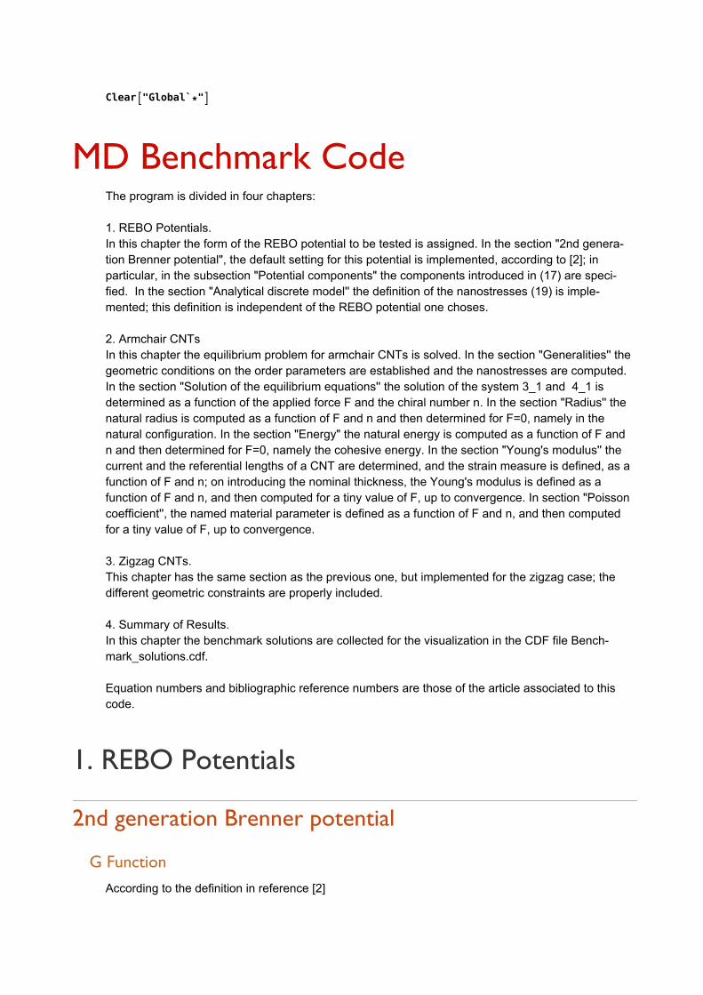
MD Benchmark CodeThe program is divided in four chapters:

1. REBO Potentials.In this chapter the form of the REBO potential to be tested is assigned. In the section "2nd genera-tion Brenner potential", the default setting for this potential is implemented, according to [2]; in particular, in the subsection "Potential components" the components introduced in (17) are speci-fied. In the section "Analytical discrete model'' the definition of the nanostresses (19) is imple-mented; this definition is independent of the REBO potential one choses.

2. Armchair CNTsIn this chapter the equilibrium problem for armchair CNTs is solved. In the section "Generalities'' the geometric conditions on the order parameters are established and the nanostresses are computed. In the section "Solution of the equilibrium equations'' the solution of the system 3_1 and 4_1 is determined as a function of the applied force F and the chiral number n. In the section "Radius'' the natural radius is computed as a function of F and n and then determined for F=0, namely in the natural configuration. In the section "Energy" the natural energy is computed as a function of F and n and then determined for F=0, namely the cohesive energy. In the section "Young's modulus'' the current and the referential lengths of a CNT are determined, and the strain measure is defined, as a function of F and n; on introducing the nominal thickness, the Young's modulus is defined as a function of F and n, and then computed for a tiny value of F, up to convergence. In section "Poisson coefficient'', the named material parameter is defined as a function of F and n, and then computed for a tiny value of F, up to convergence.

3. Zigzag CNTs.This chapter has the same section as the previous one, but implemented for the zigzag case; the different geometric constraints are properly included.

4. Summary of Results.In this chapter the benchmark solutions are collected for the visualization in the CDF file Bench-mark_solutions.cdf.

Equation numbers and bibliographic reference numbers are those of the article associated to this code.

1. REBO Potentials

2nd generation Brenner potential

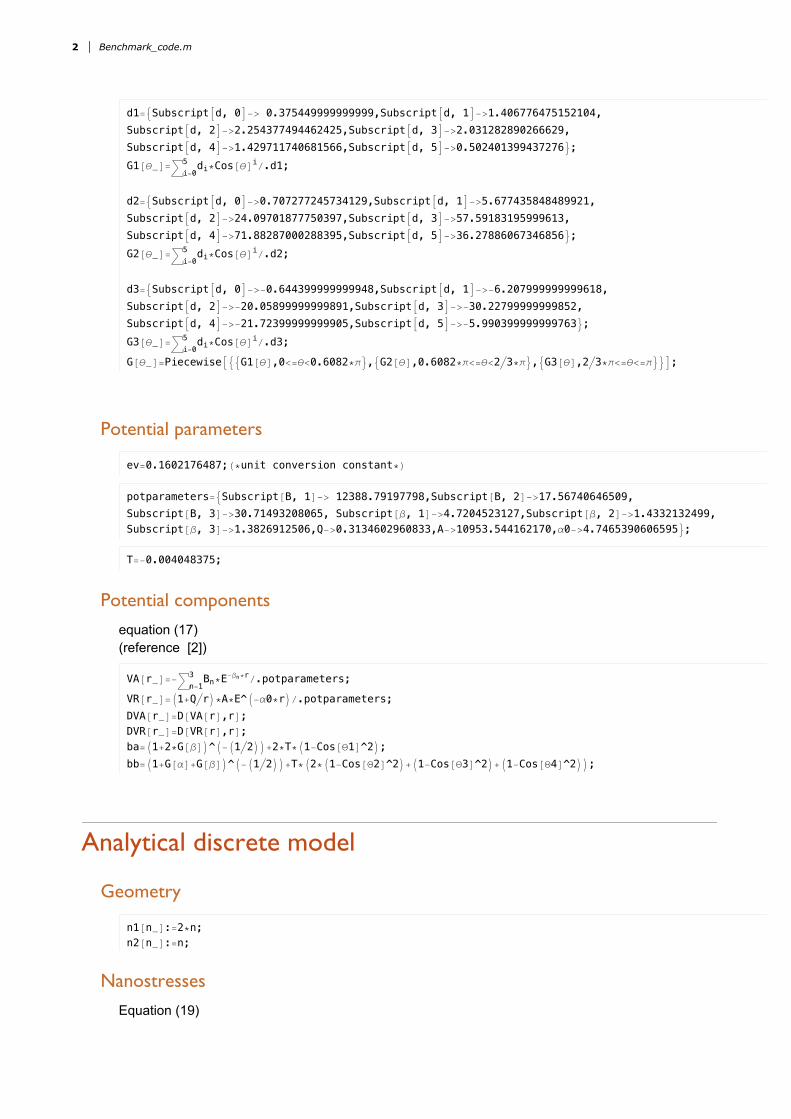
G Function

According to the definition in reference [2]

d1=Subscriptd, 0-−> 0.375449999999999,Subscriptd, 1-−>1.406776475152104,Subscriptd, 2-−>2.254377494462425,Subscriptd, 3-−>2.031282890266629,Subscriptd, 4-−>1.429711740681566,Subscriptd, 5-−>0.502401399437276;G1[θ_]=i=0

5 di*⋆Cos[θ]i/∕.d1;

d2=Subscriptd, 0-−>0.707277245734129,Subscriptd, 1-−>5.677435848489921,Subscriptd, 2-−>24.09701877750397,Subscriptd, 3-−>57.59183195999613,Subscriptd, 4-−>71.88287000288395,Subscriptd, 5-−>36.27886067346856;G2[θ_]=i=0

5 di*⋆Cos[θ]i/∕.d2;

d3=Subscriptd, 0-−>-−0.644399999999948,Subscriptd, 1-−>-−6.207999999999618,Subscriptd, 2-−>-−20.05899999999891,Subscriptd, 3-−>-−30.22799999999852,Subscriptd, 4-−>-−21.72399999999905,Subscriptd, 5-−>-−5.990399999999763;G3[θ_]=i=0

5 di*⋆Cos[θ]i/∕.d3;

G[θ_]=PiecewiseG1[θ],0<=θ<0.6082*⋆π,G2[θ],0.6082*⋆π<=θ<23*⋆π,G3[θ],23*⋆π<=θ<=π;

Potential parameters

ev=0.1602176487;(*⋆unit conversion constant*⋆)

potparameters=Subscript[B, 1]-−> 12388.79197798,Subscript[B, 2]-−>17.56740646509,Subscript[B, 3]-−>30.71493208065, Subscript[β, 1]-−>4.7204523127,Subscript[β, 2]-−>1.4332132499,Subscript[β, 3]-−>1.3826912506,Q-−>0.3134602960833,A-−>10953.544162170,α0-−>4.7465390606595;

T=-−0.004048375;

Potential components

equation (17)(reference [2])

VA[r_]=-−n=13 Bn*⋆E-−βn*⋆r/∕.potparameters;

VR[r_]=1+Qr*⋆A*⋆E^-−α0*⋆r/∕.potparameters;DVA[r_]=D[VA[r],r];DVR[r_]=D[VR[r],r];ba=1+2*⋆G[β]^-−12+2*⋆T*⋆1-−Cos[Θ1]^2;bb=1+G[α]+G[β]^-−12+T*⋆2*⋆1-−Cos[Θ2]^2+1-−Cos[Θ3]^2+1-−Cos[Θ4]^2;

Analytical discrete model

Geometry

n1[n_]:=2*⋆n;n2[n_]:=n;

Nanostresses

Equation (19)

2 Benchmark_code.m

σa=DVR[a]+ba*⋆DVA[a];σb=DVRb+bb*⋆DVAb;τα=Dbb,α*⋆VAb;τβ=14*⋆Dba,β*⋆VA[a]+2*⋆Dbb,β*⋆VAb;

T1=12*⋆Dba,Θ1*⋆VA[a];T2=12*⋆Dbb,Θ2*⋆VAb;T3=Dbb,Θ3*⋆VAb;T4=Dbb,Θ4*⋆VAb;

2. Armchair CNTs

Generalities

Geometric constraints

Reference [1]

ϕ[n_]:=πn1[n];

β[n_]:=ArcCos-−Cosα2*⋆Cos[ϕ[n]];Θ1[n_]:=2*⋆ArcSinCosα2*⋆Sin[ϕ[n]]Sin[β[n]];

Θ2[n_]:=ArcSinSin[ϕ[n]]Sin[β[n]];Θ3[n_]:=2*⋆Θ2[n];Θ4[n_]:=0;

σan[n_]:=σa/∕.β-−>β[n],Θ1-−>Θ1[n],Θ2-−>Θ2[n],Θ3-−>Θ3[n],Θ4-−>Θ4[n]σbn[n_]:=σb/∕.β-−>β[n],Θ1-−>Θ1[n],Θ2-−>Θ2[n],Θ3-−>Θ3[n],Θ4-−>Θ4[n]ταn[n_]:=τα/∕.β-−>β[n],Θ1-−>Θ1[n],Θ2-−>Θ2[n],Θ3-−>Θ3[n],Θ4-−>Θ4[n]τβn[n_]:=τβ/∕.β-−>β[n],Θ1-−>Θ1[n],Θ2-−>Θ2[n],Θ3-−>Θ3[n],Θ4-−>Θ4[n]T1n[n_]:=T1/∕.β-−>β[n],Θ1-−>Θ1[n],Θ2-−>Θ2[n],Θ3-−>Θ3[n],Θ4-−>Θ4[n]T2n[n_]:=T2/∕.β-−>β[n],Θ1-−>Θ1[n],Θ2-−>Θ2[n],Θ3-−>Θ3[n],Θ4-−>Θ4[n]T3n[n_]:=T3/∕.β-−>β[n],Θ1-−>Θ1[n],Θ2-−>Θ2[n],Θ3-−>Θ3[n],Θ4-−>Θ4[n]T4n[n_]:=T4/∕.β-−>β[n],Θ1-−>Θ1[n],Θ2-−>Θ2[n],Θ3-−>Θ3[n],Θ4-−>Θ4[n]

Solution of the equilibrium equationssolA[F_,n_]:=FindRootσan[n]==0,σbn[n]-−Fn1[n]*⋆Sinα2==0,ταn[n]+2*⋆D[β[n],α]*⋆τβn[n]+D[Θ1[n],α]*⋆T1n[n]+2*⋆D[Θ2[n],α]*⋆T2n[n]+D[Θ3[n],α]*⋆T3n[n]-−12*⋆Fn1[n]*⋆b*⋆Cosα2==0,a,1.4,b,1.4,α,2

RadiusReference [1]

ρa[n_]:=b2*⋆Cosα2+a2*⋆Cos[ϕ[n]]Sin[ϕ[n]];

ρ[n_]:=Sqrtρa[n]^2+a^24;rA[F_,n_]:=ρ[n]10/∕.solA[F,n];(*⋆radius in nm*⋆)

Benchmark_code.m 3

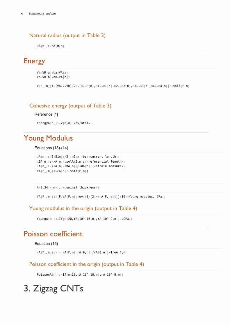
Natural radius (output in Table 3)

ρA[n_]:=rA[0,n]

Energy Va=VR[a]+ba*⋆VA[a];Vb=VRb+bb*⋆VAb;

V[F_,n_]:=Va+2*⋆Vb2/∕.β-−>β[n],Θ1-−>Θ1[n],Θ2-−>Θ2[n],Θ3-−>Θ3[n],Θ4-−>Θ4[n]/∕.solA[F,n]

Cohesive energy (output of Table 3)

Reference [1]

EnergyA[n_]:=V[0,n](*⋆evatom*⋆)

Young ModulusEquations (13)-(14)

λA[n_]:=2*⋆Sinα2*⋆n2[n]*⋆b;(*⋆current length*⋆)λ0A[n_]:=λA[n]/∕.solA[0,n];(*⋆referential length*⋆)ϵA[n_]:=λA[n]-−λ0A[n]λ0A[n];(*⋆strain measure*⋆)eA[F_,n_]:=ϵA[n]/∕.solA[F,n];

t=0.34(*⋆nm*⋆);(*⋆nominal thickness*⋆)

YA[F_,n_]:=FeA[F,n]*⋆ev*⋆12*⋆π*⋆rA[F,n]*⋆t*⋆10(*⋆Young modulus, GPa*⋆)

Young modulus in the origin (output in Table 4)

YoungA[n_]:=If[n<20,YA[10^-−10,n],YA[10^-−9,n]](*⋆GPa*⋆)

Poisson coefficientEquation (15)

νA[F_,n_]:=-−rA[F,n]-−rA[0,n]rA[0,n]*⋆1eA[F,n]

Poisson coefficient in the origin (output in Table 4)

PoissonA[n_]:=If[n<20,νA[10^-−10,n],νA[10^-−9,n]]

3. Zigzag CNTs

Generalities

4 Benchmark_code.m

Generalities

Geometric constraints

Reference [1]

ϕz[n_]:=π/∕n;

βz[n_]:=π-−ArcSinSinα2Cosϕz[n]2;Θ1z[n_]:=ϕz[n];Θ2z[n_]:=ArcSinSin[βz[n]]*⋆Sin[ϕz[n]]Sin[α];Θ3z[n_]:=0;Θ4z[n_]:=2*⋆Θ2z[n];

σaz[n_]:=σa/∕.β-−>βz[n],Θ1-−>Θ1z[n],Θ2-−>Θ2z[n],Θ3-−>Θ3z[n], Θ4-−>Θ4z[n]σbz[n_]:=σb/∕.β-−>βz[n],Θ1-−>Θ1z[n],Θ2-−>Θ2z[n],Θ3-−>Θ3z[n], Θ4-−>Θ4z[n]ταz[n_]:=τα/∕.β-−>βz[n],Θ1-−>Θ1z[n],Θ2-−>Θ2z[n],Θ3-−>Θ3z[n], Θ4-−>Θ4z[n]τβz[n_]:=τβ/∕.β-−>βz[n],Θ1-−>Θ1z[n],Θ2-−>Θ2z[n],Θ3-−>Θ3z[n], Θ4-−>Θ4z[n]T1z[n_]:=T1/∕.β-−>βz[n],Θ1-−>Θ1z[n],Θ2-−>Θ2z[n],Θ3-−>Θ3z[n], Θ4-−>Θ4z[n]T2z[n_]:=T2/∕.β-−>βz[n],Θ1-−>Θ1z[n],Θ2-−>Θ2z[n],Θ3-−>Θ3z[n], Θ4-−>Θ4z[n]T3z[n_]:=T3/∕.β-−>βz[n],Θ1-−>Θ1z[n],Θ2-−>Θ2z[n],Θ3-−>Θ3z[n], Θ4-−>Θ4z[n]T4z[n_]:=T4/∕.β-−>βz[n],Θ1-−>Θ1z[n],Θ2-−>Θ2z[n],Θ3-−>Θ3z[n], Θ4-−>Θ4z[n]

Solution of the equilibrium equationssolZ[F_,n_]:=FindRootσaz[n]-−Fn2[n]==0,σbz[n]+F2*⋆n2[n]*⋆Cos[βz[n]]==0,ταz[n]+2*⋆D[βz[n],α]*⋆τβz[n]+2*⋆D[Θ2z[n],α]*⋆T2z[n]+D[Θ4z[n],α]*⋆T4z[n]-−12*⋆Fn2[n]*⋆b*⋆D[βz[n],α]*⋆Sin[βz[n]]==0,a,1.4,b,1.4,α,2

RadiusReference [1]

rz[n_]:=Sin[βz[n]]2*⋆Sinϕz[n]2*⋆b;

r[F_,n_]:=rz[n]10/∕.solZ[F,n];(*⋆radius in nm*⋆)

Natural radius (output in Table 3)

ρZ[n_]:=r[0,n](*⋆nm*⋆)

EnergyVZ[F_,n_]:=Va+2*⋆Vb2/∕.β-−>βz[n],Θ1-−>Θ1z[n],Θ2-−>Θ2z[n],Θ3-−>Θ3z[n], Θ4-−>Θ4z[n]/∕.solZ[F,n]

Cohesive energy (output in Table 3)

EnergyZ[n_]:=VZ[0,n](*⋆evatom*⋆)

Young Modulus

Benchmark_code.m 5

Young ModulusEquations (13)-(14)

λZ[n_]:=1-−ba*⋆Cos[βz[n]]*⋆n1[n]*⋆a;(*⋆current length*⋆)λ0Z[n_]:=λZ[n]/∕.solZ[0,n];(*⋆referential length*⋆)ϵZ[n_]:=λZ[n]-−λ0Z[n]λ0Z[n];(*⋆strain measure*⋆)eZ[F_,n_]:=ϵZ[n]/∕.solZ[F,n];

YZ[F_,n_]:=FeZ[F,n]*⋆ev*⋆12*⋆π*⋆r[F,n]*⋆t*⋆10(*⋆Young modulus,GPa*⋆)

Young modulus in the origin (output in Table 4)

YoungZ[n_]:=YZ[10^-−8,n](*⋆GPa*⋆)

Poisson ratioEquation (15)

ν[F_,n_]:=-−r[F,n]-−r[0,n]r[0,n]*⋆1eZ[F,n]

Poisson coefficient in the origin (output in Table 4)

PoissonZ[n_]:=ν[10^-−8,n]

4. Summary of ResultsRadius[0,n_]:=ρA[n]Radius[1,n_]:=ρZ[n]Energy[0,n_]:=EnergyA[n]Energy[1,n_]:=EnergyZ[n]Young[0,n_]:=YoungA[n]Young[1,n_]:=YoungZ[n]Poisson[0,n_]:=PoissonA[n]Poisson[1,n_]:=PoissonZ[n]

Creation of the shell for cdf file

ManipulateColumn NumberFormRadius[q,n],4 "radius [nm]:",NumberForm[Energy[q,n],5] "cohesive energyNumberForm[Young[q,n],7] "Young modulus [GPa]:", NumberForm[Poisson[q,n],4] "Poisson coefficient

Left,", ",q,0,"show",0-−>"armchair",1-−>"zigzag",Setter,n,3,30,AutorunSequencing-−>1,2,TrackedSymbols:>{q,n},ControlPlacement-−>Top,SaveDefinitions-−>True,ControlType-−>InputField

6 Benchmark_code.m

Benchmark solutions for REBO potentialsGet["/∕mydirectory/∕Benchmark_code.m"]

show armchair zigzag

n 3

radius [nm]: 0.2111cohesive energy [ev/∕atom]: -−7.0137Young modulus [GPa]: 890.5525Poisson coefficient: 0.149

Instructions1. Load the package “Benchmark_code.m” inserting the directory in “Get” command and press “Shift+Enter”2. Choose armchair or zigzag CNTs3. Choose the chiral number n4. Press Enter to visualize the benchmark results

NoteThe code is set for 2nd generation Brenner potential. In order to check another REBO potential, it is necessary to define the proper potential functions and all the corresponding parameters in the “Benchmark_code.m” file.