computer vision for computer graphics - faculty of ict …sspi3/computervision-pt1.pdf · ·...

14/04/2010

1

Computer Vision

for Computer Graphics

Mark Borg

Computer Vision & Computer Graphics I

Mark Borg 28 March 2010 CSA2207

Computer Vision

Understanding the “content” of an image (normaly by creating

a “model” of the observed scene)

Computer Graphics

Creating an image using a computer “model”

(synthesis) (analysis)

14/04/2010

2

Computer Vision & Computer Graphics II


Recent confluence between computer vision (CV) and

computer graphics (CG)

Computer

Vision

Computer

Graphics

Outline


We will look at the following CV areas:

Stereovision

Recovering depth information

Stereo correspondence problem

Multi-view imaging and the Plenoptic function

Applications to CG:

3D Model Acquisition

View Morphing, “bullet time” effect

Automated Visual Surveillance

Motion Detection

Background Subtraction techniques

Object Tracking

Applications to CG:

Motion Capture

Basis for Behaviour Recognition in HCI interfaces, Project Natal

14/04/2010

3

Stereo Vision


“Stereo Vision” generally means two synchronised cameras or

eyes capturing images

Allows recovery of depth information / sensation of depth

(stereo vision = stereoscopic vision = stereopsis)

Parallax effect


Each eye has a slightly different view of the world

Nearby objects have a larger parallax than more distant objects

14/04/2010

4

Depth from Binocular Disparity


Binocular disparity:

The difference in image location of an object seen by the left and right

eyes, resulting from the horizontal separation between the eyes.

Depth from Binocular Disparity II


Binocular disparity:

The difference in image location of an object seen by the left and right

eyes, resulting from the horizontal separation between the eyes.

disparity d

14/04/2010

5

Camera model


„Pinhole‟ camera model

Simplified camera model; most often used in CV.

No lens; just a single very small aperture (infinitely small).

Models perspective projection.

Assumes all light rays pass through a single point (the „pinhole‟).

Assumes the View Volume (camera‟s FOV) is an infinite pyramid.

camera

View volume (camera‟s FOV)

image plane

pinhole

Camera model II


Limitations of the pinhole camera model:

Depth-of-field effects and light attenuation ignored in this model.

View volume is not really infinite.

camera


image plane

pinhole

14/04/2010

6

Camera model III


Single Viewpoint Constraint

Image plane is situated at a distance ƒ (the focal length) from the pinhole.

The pinhole is also called the focal point, or centre of projection, or lens centre.

A camera with a single centre of projection is called a central projection camera (central camera for short) and obey the single viewpoint constraint.

Such a camera „sees‟ the world from a single point (has a single viewpoint).


image plane focal length f

pinhole / focal point

/ centre of projection

Camera model IV


optical axis focal point

focal length f

image plane

14/04/2010

7

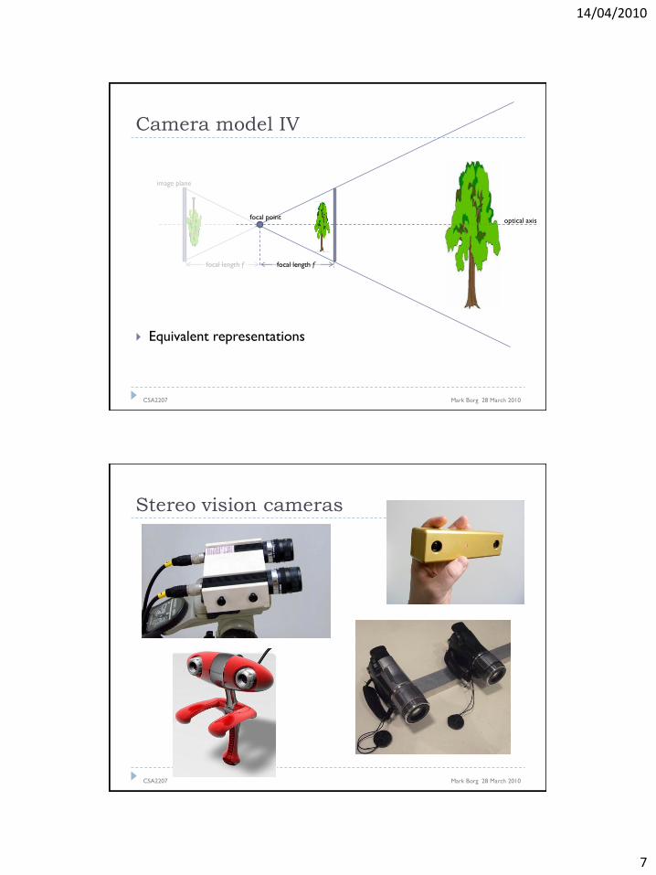
Camera model IV


Equivalent representations

optical axis focal point

focal length f focal length f

image plane

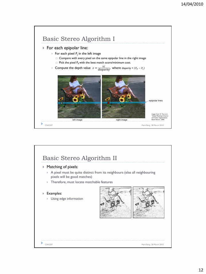
Stereo vision cameras


14/04/2010

8

Depth from Binocular Disparity III


Ratio of sides of similar triangles:

𝑃𝐿

ƒ =

−1

2𝑏 + 𝑥

𝑍

α

α

baseline b

P(x,y,z)

FL FR

PL PR

z=0

x=0 xL=0 xR=0

ƒ

z




𝑃𝐿

ƒ =

−1

2𝑏 + 𝑥

𝑍

𝑃𝑅

ƒ =

1

2𝑏 + 𝑥

𝑍

α

α

baseline b

P(x,y,z)

FL FR

PL PR

z=0

x=0 xL=0 xR=0

ƒ

z

β

β

14/04/2010

9




𝑃𝐿

ƒ =

−1

2𝑏 + 𝑥

𝑍

𝑃𝑅

ƒ =

1

2𝑏 + 𝑥

𝑍

𝑧 𝑃𝑅 − 𝑃𝐿 = 𝑏𝑓

𝑧 =𝑏𝑓

𝑃𝑅−𝑃𝐿

where 𝑃𝑅 − 𝑃𝐿 is the disparity

α

α

baseline b

P(x,y,z)

FL FR

PL PR

z=0

x=0 xL=0 xR=0

ƒ

z

β

β

Depth from Binocular Disparity IV


𝑧 =𝑏𝑓

𝑃𝑅−𝑃𝐿

where 𝑃𝑅 − 𝑃𝐿 is the disparity

𝑧 ∝ 1

𝑑𝑖𝑠𝑝𝑎𝑟𝑖𝑡𝑦

As disparity 𝑃𝑅 − 𝑃𝐿 → 0,

depth z → ∞

In reality, depth resolution

determined by minimum disparity

baseline b

P(x,y,z)

FL FR

PL PR

z=0

x=0

ƒ

z

14/04/2010

10

Choosing the stereo baseline


What‟s the optimal baseline?

Small baseline:

Smaller disparities → larger depth error; limited depth range.

one pixel

All these points

project to the same

pixel pair

Smaller disparity

Large baseline Small baseline

Choosing the stereo baseline


What‟s the optimal baseline?

Small baseline:

Smaller disparities → larger depth error; limited depth range.

Large baseline:

Less FOV intersection → less scene points for which depth can be measured; more difficult search problem.

Examples:

Human binocular vision: baseline = ~6cm; depth estimation = up to ~10m.

Stellar parallax estimation: baseline = Earth‟s orbital diameter; depth estimation = up to ~100 LY.

Large baseline Small baseline

Less FOV

intersection

Points for which

no depth estimation

can be done

14/04/2010

11

Correspondence Problem


Basic stereo algorithm:

For a pixel PL in the left image

Find the matching pixel PR in the right image

Compute the depth value 𝑧 =𝑏𝑓

disparity, where disparity = 𝑃𝑅 − 𝑃𝐿

Matching the points is a

hard problem

Called the (Stereo) Correspondence Problem

Can reduce the search problem from 2D to 1D by using

constraints from epipolar geometry

Right image

Left image

PL ?

Epipolar Geometry


Epipolar plane

Scene point P + image points PL, PR + camera focal points

Epipolar line

Intersection of epipolar plane with image plane of the camera

Epipolar Constraint

Given a point PL, the corresponding point PR will always occur along the conjugate epipolar line.

Reduces the search problem to a 1D search along conjugate epipolar lines.

For the camera configuration above, the conjugate epipolar lines correspond to the same image rows.

fL fR

Epipolar

plane

P

PL PR

Epipolar line

Epipolar line

14/04/2010

12

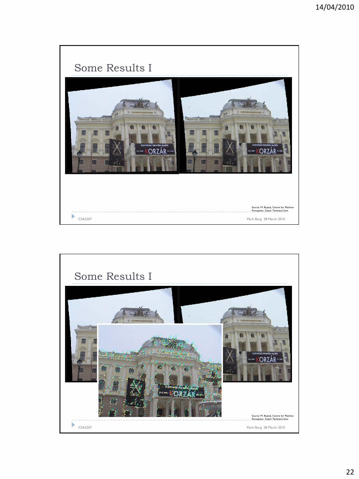
Basic Stereo Algorithm I


For each epipolar line:

For each pixel PL in the left image

Compare with every pixel on the same epipolar line in the right image

Pick the pixel PR with the best match score/minimum cost.

Compute the depth value 𝑧 =𝑏𝑓

disparity, where disparity = 𝑃𝑅 − 𝑃𝐿

left image right image

Images from: H. Tao et al.,

“Global Matching Criterion

and Colour Segmentation

Based Stereo”, 2000.

epipolar lines

Basic Stereo Algorithm II


Matching of pixels:

A pixel must be quite distinct from its neighbours (else all neighbouring

pixels will be good matches)

Therefore, must locate matchable features

Examples:

Using edge information

14/04/2010

13

Basic Stereo Algorithm II


Matching of pixels:

A pixel must be quite distinct from its neighbours (else all neighbouring

pixels will be good matches)

Therefore, must locate matchable features

Examples:

Using edge information

Using corner features

Using region correlation

End result:

Normally a subset of pixels/features are selected for matching and depth

computation.

Depth at other points can be estimated via interpolation techniques.

Basic Stereo Algorithm III


3D point cloud

Can be sparse or dense, depending on the features used for

matching

Can be transformed into a surface model

Via depth or shape interpolation techniques

Mesh fitting

One common method: Dalaunay Triangulation

14/04/2010

14

Some Results I


left image right image depth map

Images from: H. Tao et al.,

“Global Matching Criterion

and Colour Segmentation

Based Stereo”, 2000.

Some Results II


depth map

rendered view

Note the „holes‟ caused by

scene occlusions. These

scene points are hidden

from both cameras.

14/04/2010

15

Some Results III


Disparity map

Stereo vision for robot navigation.

Source: Jet Propulsion Laboratory, NASA.

Some Results III


Source: Project IS-3D, Centre

for Machine Perception, Czech

Academy of Sciences, 2008.

14/04/2010

16

Some Results III





Disparity map

Some Results III





Disparity map 3D Point cloud

14/04/2010

17

Some Results III





Disparity map 3D Point cloud

3D Model

Parallel camera configuration


Cameras oriented parallel to each other

Conjugate epipolar lines map to the same image rows

Requires precise positioning and orientation of the cameras

Difficult to achieve in practice

fL fR

Epipolar

plane

P

Epipolar line

Epipolar line PL PR

14/04/2010

18

Converging camera configuration I


Cameras no longer oriented parallel to each other.

Conjugate epipolar lines no longer correspond to image rows and are not even parallel to each other.

Each focal point projects onto a distinct point into the other camera‟s image plane

These are called the epipoles (or epipolar points)

All epipolar lines in an image must intersect the epipole.

P

fL fR

PL PR

Epipolar

plane Epipolar line

Epipole eL Epipole eR

Converging camera configuration II


How can we find the epipolar lines since they are not parallel or image rows?

Fundamental matrix 𝐹

This is a 3x3 matrix that relates any point PL with PR

Epipolar Constraint can be expressed mathematically:

𝑃𝐿𝑇 𝐹 𝑃𝑅 = 0

Also, multiplying the Fundamental matrix with a point gives the corresponding epipolar line in the other image:

𝐹 𝑃𝐿 = 𝐿𝑅 and 𝐹𝑇 𝑃𝑅 = 𝐿𝐿

Epipolar line LL

P

fL fR

PL PR

Epipolar

plane Epipolar line LR


14/04/2010

19

Fundamental Matrix


Given 2 corresponding image points 𝑝 = 𝑥, 𝑦 and 𝑝′ = 𝑥′, 𝑦′

Epipolar constraint: 𝑥′ 𝑦′ 1 𝐹

𝑥𝑦1

= 0

F =

0 −𝑒′𝑤 𝑒′𝑦𝑒′𝑤 0 −𝑒′𝑥

−𝑒′𝑦 𝑒′𝑥 0

× 𝑃′𝑃+

where 𝑒′ = 𝑒′𝑥 𝑒′𝑦 𝑒′𝑤 is the epipole in the right image,

𝑃, 𝑃′ are the camera projection matrices,

and 𝑃+ is the pseudo-inverse of matrix P.

For the parallel camera configuration, the fundamental matrix F simplifies to:

0 0 00 0 −10 1 0

Hence: 𝑥′𝑦′10 0 00 0 −10 1 0

𝑥𝑦1

= 0 → 𝑦′ = 𝑦

and the epipoles are: 𝑒 = 𝑒′ = [1 0 0] (at infinity).

P

Converging camera configuration III


Advantage:

No need for precise positioning and orientation of the cameras.

Disadvantage:

Difficult to perform a search along epipolar lines during pixel matching.

Solution:

Perform stereo image rectification.

fL fR

PL PR

Epipolar

plane Epipolar line LR


Epipolar line LL

14/04/2010

20

Stereo Image Rectification I


Rectification is the process of re-

sampling the stereo images so

that the epipolar lines correspond

to image rows.

fL

fR

Stereo Image Rectification I


Rectification is the process of re-

sampling the stereo images so

that the epipolar lines correspond

to image rows.

Images re-projected onto a

common plane parallel to the line

between focal points.

fL

fR

14/04/2010

21

Stereo Image Rectification II


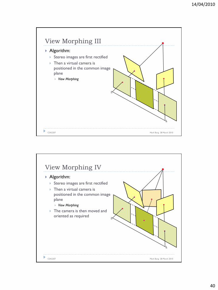
Some Results I


Source: M. Bujnak, Centre for Machine

Perception, Czech Technical Univ.

14/04/2010

22

Some Results I




Some Results I




14/04/2010

23

Some Results I




Some Results II


3D disparity

point cloud

Disparity

map

Synthetic

image from

disparity

map

Source:

www.metria.es

14/04/2010

24

Some Results III


Source: Group of Robotics and Cognitive Systems,

Democritus University of Thrace, Greece.

Some Results IV


Source: Marco Mengelkoch, Universitat Koblenz.

14/04/2010

25

Depth from a single camera I


What about this guy?

Can we recover (some) depth information using only one sensor/camera?

Depth from a single camera II


Human vision does not rely solely on binocular vision for depth estimation

Other visual cues can be used for 3D

In CV, “Shape from X” techniques:

Shading

C. Wu et al., “Shape-from-Shading under Near Point

Lighting and Partial views for Orthopeadic Endoscopy”,

2007.

14/04/2010

26

Depth from a single camera III





Shading

Texture

“The Visual Cliff”, William Vandivert, 1960.

Depth from a single camera IV





Shading

Texture

Focus

T. Aydin et al., “A New Adaptive Focus Measure for

Shape From Focus”, 2008.

14/04/2010

27

Depth from a single camera V





Shading

Texture

Focus

Motion - motion parallax

- optical flow

& many others…

(1) T. Sato et al., “Reconstuction of 3-D Models of an Outdoor Scene from Multiple Image Sequences

by Estimating Camera Motion Parameters”. (2) K. Kutulakos, “A Theory of Shape by Space Carving”.

Depth from a single camera VI





Shading

Texture

Focus

Motion

& many others…

Structured light &

laser scanning

(1) L. Zhang et al., “Rapid Shape Acquisition

Using Colour Structured Light and Multi-pass

Dynamic Programming”

(2) The Digital Michelangelo project, Stanford

Univ.

http://www.washington.edu/newsroom/news/images/David.jpg

14/04/2010

28

Depth from a single camera VII





Shading

Texture

Focus

Motion

& many others…

Structured light &

laser scanning

Time-of-flight

cameras PMDT Technologies, GmbH.

Multi-View Stereo


Monocular depth estimation

Stereo Vision systems

2 camera systems (Binocular systems)

Can extend the same process and algorithms to:

3 camera systems (Trinocular systems)

4 camera systems and more…

Multi-View Stereo systems

10 stereo reconstructions, MER Opportunity Rover.

Source: ExoMars PanCam 3D Vision Team

Commercial 2- and 3-camera

systems, PointGrey Inc.

14/04/2010

29

Multi-View Stereo II


Finding correspondences between adjacent rectified image pairs

Pair-wise disparity estimation

Fusing all the estimates into one 3D model

Bundle Adjustment algorithm Derived from the idea of “bundles” of light

rays

Iteratively refining the 3D coordinates of the scene points (as well as the cameras‟ parameters) by minimising the re-projection error between the image locations of the observed and predicted image points

Minimisation through the use of the Levenberg-Marquardt algorithm

Triggs et al. “Bundle Adjustment – A Modern

Synthesis”, 1999.

Example I


Photosynth (http://photosynth.net)

Extracts distinctive feature points in each image, matching these across the image set, and

automatically reconstructs a partial 3D model of the scene and camera geometry.

The sparse 3D model consists of a point cloud, line segments, and low-resolution

“watercolour washes”.

14/04/2010

30

Example I







Example I







14/04/2010

31

Example I







Example I







14/04/2010

32

Example I







Example II


Urban 3D modelling project using multi-camera systems (The University of North Carolina at

Chapel Hill).

Uses a 4-camera stereovision system mounted on a car

Uses a multi-way plane sweeping stereovision algorithm

4-camera system

14/04/2010

33

Example II



Chapel Hill).



4-camera system

Reconstructed 3D view of part of a street

Example II



Chapel Hill).



4-camera system


View from above and details of 2 buildings

14/04/2010

34

Example II



Chapel Hill).



4-camera system


View from above and details of 2 buildings

The Plenoptic function I


Plenoptic:

Plenus = complete/full + Optic = light

7-dimensional function:

𝑃 𝜃, 𝜙, 𝑉𝑥, 𝑉𝑦, 𝑉𝑧, 𝑡, 𝜆

To measure the plenoptic function one can imagine:

Placing an imaginary eye at every possible location 𝑉𝑥, 𝑉𝑦, 𝑉𝑧

Recording the intensity of light at every angle 𝜃, 𝜙

For every wavelength 𝜆

At every time 𝑡

The Plenoptic function is an idealised

concept of a “complete view of the

world”

14/04/2010

35

The Plenoptic function II


𝑃 𝜃, 𝜙, 𝑉𝑥, 𝑉𝑦, 𝑉𝑧 , 𝑡, 𝜆

We can only sample the plenoptic function at a finite number of points in space (N-camera system)

What‟s the use of the plenoptic function? Allows us to think about novel ways of

sampling/navigating in this 7D space

Given images acquired from N cameras (sparse sampling), can we observe the scene by moving

freely in space? i.e., create a virtual camera, let it move along

some trajectory/manifold in space, thus creating a so-called free-viewpoint video? Need to be able to synthesise new views

can we let the virtual camera move in space while freezing time? i.e., create a so-called “bullet time” special

effect?











effect?

14/04/2010

36











effect?











effect?

14/04/2010

37











effect?

Note that we are not interested in rendering virtual

views using 3D models here. But just using the

acquired image data and measured pixel depth map.

View Morphing I


Image A

Camera A

Image B

Camera B

Source: S. Seitz, C. Dyer, 1996.

14/04/2010

38

View Morphing I


Virtual camera

Virtual camera

Image A

Camera A

Image B

Camera B


View Morphing I


Virtual camera

View morphing

Morphed View

Virtual camera

Image A

Camera A

Image B

Camera B


14/04/2010

39

View Morphing I


Virtual camera

View morphing

Morphed View

Virtual camera

Image A

Camera A

Image B

Camera B

Note that view morphing is not image morphing.


Image morphing is not 3D shape preserving.

View Morphing II


Algorithm:

Stereo images are first rectified

fL

fR

14/04/2010

40

View Morphing III


Algorithm:


Then a virtual camera is

positioned in the common image

plane

View Morphing

fL

fR

View Morphing IV


Algorithm:




plane

View Morphing

The camera is then moved and

oriented as required fL

fR

14/04/2010

41

View Morphing IV


Algorithm:




plane

View Morphing

The camera is then moved and

oriented as required fL

fR


Note that we can also „acquire‟

multiple views of a single photo by

operations like mirroring. Then

perform view morphing on them. E.g.

Mona Lisa sequence:

“Bullet Time” Effect


14/04/2010

42





14/04/2010

43

Some demos


The Campanile movie

Paul Debevac, Univ. of California, Berkeley,1996.

http://www.debevac.org/campanile

ProFORMA

Qi Pan, Univ. of Cambridge, 2009.

http://mi.eng.cam.ac.uk/~qp202

Paul Debevac, 1996.

Further Information…


“Multiple View Geometry in Computer Vision”, Richard

Hartley, Andrew Zisserman, 2nd Ed., 2004.

Open Source Computer Vision Library

C++ library containing lots of CV algorithms, including stereo

vision algorithms.

http://sourceforge.net/projects/opencvlibrary/

The MSRC Stereo Vision C# SDK

Microsoft Research in Cambridge

http://research.microsoft.com/en-us/projects/i2i/default.aspx

http://sourceforge.net/projects/opencvlibrary/




computer vision for computer graphics - faculty of ict …sspi3/computervision-pt1.pdf · ·...

Documents