computer vision ece 661 homework 10 - purdue … · computer vision ece 661 homework 10 rohan...

Computer VisionECE 661 Homework 10

Rohan Sarkar ([email protected])

November 29, 2016

1. Introduction

In this assignment, we perform a 3D scene reconstruction with projective distortion usingtwo stereo images captured by an uncalibrated camera. Such a 3D reconstruction is calledprojective reconstruction. because the reconstruction is projectively distorted visually andit is related by a 4 × 4 homography to the real scene. If the scene is visually rich and wehave prior knowledge about the objects that appear in the scene, we can remove projectivedistortion, affine and similarity distortion successively.

The following steps are performed for the 3D reconstruction :

1. An initial estimate of the fundamental matrix F is found, using the manually selectedcorrespondences (minimum of 8) between the 2 images by linear least squaresoptimization and refine the fundamental matrix F using the Levenberg MarquadtMethod.

2. Using this initial estimate of F, we rectify the images to send the epipoles to infinitysuch that e= [

1 0 0]T and thereby find the Homographies for the two cameras for

this purpose, represented by H,H′.

3. Using the rectified images, the interest points on the rectified images are found usingSURF and canny edge detector.

4. After finding the interest points in the rectified images, we calculate the euclideandistance geometric error to calculate the cost function and apply the non-linear leastsquares optimization to minimize it and refine the fundamental matrix, cameramatrices and the 3D world points.

5. Finally we shall use triangulation to project the point correspondences to world 3Dand compute the 3D Scene structure from the set of correspondences for the givencamera pair (P,P′).

2. Theory and Implementation

Linear Least Squares estimation of the Fundamental Matrix

The Fundamental Matrix F is estimated using the manual correspondences (xi,x′i) that are

selected by the user.(xi,x′i) are the pixel locations in homogeneous coordinates in the left

and right image of the same world point selected by the user manually. The FundamentalMatrix F gives us the algebraic representation of the epipolar geometry which finds therelation between the corresponding points (xi,x′

i). The algebraic equation is given by

x′Ti Fxi = 0

=⇒ [u′

iui u′ivi u′

i v′iui v′ivi v′i ui vi 1]f= 0

1

From a set of n point matches, we obtain a set of linear equations of the form

A.f=

u′1u1 u′

1v1 u′1 v′1u1 v′1v1 v′1 u1 v1 1

......

......

......

......

...u′

nun u′nvn u′

n v′nun v′nvn v′n un vn 1

f= 0

where,f= [

f11 f12 f13 f21 f22 f23 f31 f32 f33]

f33 = 1

xi =[ui vi 1

]T x′i =

[u′

i v′i 1]T

Since each correspondence gives us 1 equation by solving, x′Ti Fxi = 0. Since there are 8

unknowns, we need a minimum of 8 such correspondences to use the normalized 8 pointalgorithm, which normalizes the data to improve the estimate of the Fundamental MatrixF. The steps are enumerated below:

1. Normalization : The image coordinates are transformed according to

xi =Txi x′i =T′x′i

where T and T′ are normalizing transformations consisting of a translation andscaling.The normalizing transformations T, for points xi and T′, for points x′

i for thetwo images are found such that all the pixel correspondences have 0 mean and areat a distance of

p2 from the center C1 = (0,0).

2. Linear Solution : When we have normalized all the points, we stack up all ofthem and make a matrix vector equation of the form A.f= 0.The matrix A hasall the stacked rows similar to the matrix shown above and is composed of thematches between xi and x′i. This is solved using SVD to yield the matrix F from fcorresponding to the smallest singular value of A.

3. Constraint enforcement : The rank of matrix F has to be 2. Therefore we mayneed to condition the matrix F to make its rank 2. This is done again by usingSingular Value Decomposition.So if F=UDVT , we set the smallest singular value inD equal to 0 and then denote it with DCE. So we replace F by FCE =UDCEVT suchthat det(FCE)= 0

4. Denormalization : Next, we denormalize the fundamental matrix FCE by usingthe following relation

F=T′TFCET

5. Next we compute the epipoles of the left and right images. e is the right null vectorof fundamental matrix F and e′ is the left null vector of fundamental matrix F.

F.e= 0 e′TF= 0

6. Finally we calculate the camera projection matrices in the canonical form as follows:

P= [I|0] P′ = [[e′]xF|e′]

2

Initial estimates before rectification and before refining

Initial Fundamental Matrix before images are rectified is given by :

F=1.61993193122650e−07 −8.41209003027106e−06 −0.00430054597756484

8.50415583183406e−06 −7.34816171971557e−07 −0.02879163429275440.00364100843113559 0.0295143317479700 1

Initial First Camera Projection Matrix is given by :

P=1 0 0 0

0 1 0 00 0 1 0

Initial Second Camera Projection Matrix is given by :

P′ =−1.80523197679284 −14.6332981048719 −495.774364765972 3551.87067873625−12.9323909255888 −104.831097950199 −3551.87497928223 −495.8031564002650.0302859784829609 −0.00678071280441858 −104.396385907253 1

Initial epipoles are given by :

e= 3346.99098369553−446.780313482016

1

e′ = 3551.87067873625−495.803156400265

1

Final estimates before rectification and after refining

Refined Fundamental Matrix before images are rectified is given by :

F=2.00548076986446e−07 −1.29984078437012e−05 −0.00130076977575196

1.34181204176223e−05 −5.41186060674474e−07 −0.03779429913792380.000417385932814687 0.0383884228246249 1

Refined First Camera Projection Matrix is given by :

P=1 0 0 0

0 1 0 00 0 1 0

Refined Second Camera Projection Matrix is given by :

P′ = −14.9486114725145 −21.6540815829875 −408.511137615021 2956.45213307080−0.844575731781253 −112.141710233451 −2925.19966927627 −75.29346073520630.0343340132683272 −0.00891305474721164 −111.087250279651 1

3

Refined epipoles are given by :

e= 2814.37638782766−56.6493998427590

1

e′ = 2956.45213307083−75.2934607352072

1

Final estimates after rectification

Final Fundamental Matrix after images are rectified is given by :

F=−5.69457800755607e−26 1.24071872320692e−21 8.04011778842355e−20−1.32348898008484e−22 7.85821581925376e−23 0.000214584025844281−3.81164826264435e−21 −0.000214584025844281 −0.00584613578291279

Final Rectification Homography for first image is given by :

H= 0.3537 −0.1086 131.5316

0.0111 0.5653 0.8599−0.0004 0.0001 1.0000

Final Rectification Homography for second image is given by :

H′ = 0.3750 −0.1174 141.4748

0.0145 0.5700 −0.0090−0.0003 0.0001 1.0000

4

Input Images

Figure 1: Input Images

5

Extracting Manual Correspondences

Taking the manual correspondences requires the user to click on points of interest that arepresent in both images. The advantage of this method is that it uses human knowledgeabout the corresponding points of interest that lie on the object of interest to accurately spotcorrespondences. Often it is difficult to manually extract 40 corresponding points which isrequired to rectify the image accurately.However, since this method uses human knowledge,we can use even the bare minimum number of points (minimum of 8) required to computethe fundamental matrix.I found 20 manual correspondences. However, a significant draw-back is that while humans can identify correspondences easily, human eye cannot pinpointthe exact position of the correspondences upto a pixel or sub-pixel accuracy. The accuracyof the correspondences greatly affects the result of the scene reconstruction procedure. Inmy approach, I have written a MATLAB Script find_manual_correspondence.m usingwhich I can just click on the corresponding points of interest on both the images using across-hair cursor which makes locating points easier and accurate.

Figure 2: Setup for taking Manual Correspondences

6

Figure 3: Points of Interest selected manually

Figure 4: Correspondences between points of interest selected manually

Image Rectification

In order to accurately compute our projectively distorted 3D scene structure, we mustobtain a highly refined estimate of matrix F. For this we need a considerably large numberof pixel correspondences (xi,x′

i) between the two images. For this we need to solve the’correspondence problem’. It is computationally efficient, if we can simply lookup forpixel correspondences along the same rows for each pixel in one image (if F is perfectlyestimated).In practical cases estimating F perfectly is not possible, and thus we look forcorrespondences in a small number of adjoining rows in the second image, but it stillreduces the search space considerably and hence is much more computationally efficient.This is done by sending the epipoles in both the images to infinity. We compute thehomographies H and H′ to send the epipoles e and e′ to infinity. The steps are enumerated

7

below:

Estimating Homography H’ to send epipole e’ to ∞ along x axis

1. The second image center is shifted to origin using the transformation T1 to make theapplication of rotation easier.

2. The angle of the epipole w.r.t positive x-axis is found by using the formula

θ = tan−1(− height(image)/2− e2(y)

width(image)/2− e2(x)

)3. The entire image is rotated by this angle θ so that epipole goes to x-axis

e′ = f

01

4. Then the Homography G is applied to send the epipole to infinity along the x axis.

G=

1 0 00 1 0− 1

f 0 1

e′ = f

00

5. Finally the image center is translated back to its original center point using the

transformation T2.

6. The overall Homography to be applied onto the second image to accomplish all thesetasks is then given by

H′ =T2GRT1

Estimating Homography H to send epipole e to ∞ along x axis

We want the corresponding epipolar lines to be on the same rows. The homoraphy H forthe first image is found using a linear least squares minimization procedure to minimizethe sum of squares distances given by∑

idistance(Hxi,H′x′

i)

. This is done in the following steps which are enumerated below:

1. This is done by finding M such that F= [[e′]xM].

M=P′P+

2. We select a,b, c such that they minimize the following sum of squares:∑i

(axi +byi + c− x′ i)2 xi =H0xi x′i =H2x′i

8

3. We find the hollowing Homographies

H0 =H2M HA =a b c

0 1 00 0 1

4. The overall Homography to be applied onto the first image to accomplish all these

tasks is then given byH=HAH0

2.1 Output of Image Rectification

Figure 5: Input Images

Figure 6: Rectified Images

9

Interest Point Detection

After rectification of the images, we look for interest points in the two images using SURFand Canny Edge Detector. Finding large number of interest points and correspondencesbetween the stereo images is important for proper 3D Reconstruction. Using rectifiedimages solves the ’correspondence problem’, or in other words, all the correspondinginterest points are usually on the same rows or within a small number of adjoining rows.The procedure to find the interest points and the point correspondences is explained below.

SURF Features

Speeded Up Robust Features (SURF) is a local feature detector and descriptor. It is usedfor tasks such as object recognition, image registration, classification or 3D reconstruction.SURF is several times faster and more robust than SIFT.

1. To detect interest points, SURF uses an integer approximation of the determinantof Hessian blob detector, which can be computed with 3 integer operations on apreviously computed integral image.

S(x,y)=x∑

i=0

y∑j=0

I(i, j)

The MATLAB function detectSURFFeatures( ) is used to detect SURF featuresand returns a SURFPoints object, points, containing information about SURF fea-tures detected in the 2-D grayscale input image.

2. The 64 dimensional SURF descriptors for each of the interest points are then com-puted using the MATLAB Command extractFeatures() which returns the extractedSURF feature vectors, also known as descriptors, and their corresponding locations,from the gray scale image. These descriptors are used to find correspondences.

10

Output of SURF Feature Detection

Figure 7: Interest Points detected in the 2 Images using SURF Algorithm

Figure 8: Best 40 Visual SURF Features detected in the 2 Images using SURF Algorithm

Canny Edge Detector Features

1. Use canny edge detector to find edges in both the images using the MATLAB com-mand edge() and specifying ’canny’ while executing the function .

2. The pixels corresponding to edges are used as the interest points.

3. This results in a very large number of pixels (around 10000 points). A subset ofthese points are chosen so that we get around 1000 interest points. The points arechosen at uniform intervals(i.e. every 10 th point is chosen).This is done so that wedo not choose consecutive points lying on the same edge corresponding to edges inthe image. Otherwise we will not be able to do the 3D Reconstruction accurately.

4. My own algorithm of choosing interest points only on Object Of Interest is appliedto only choose interest points on the object and exclude all other background points

11

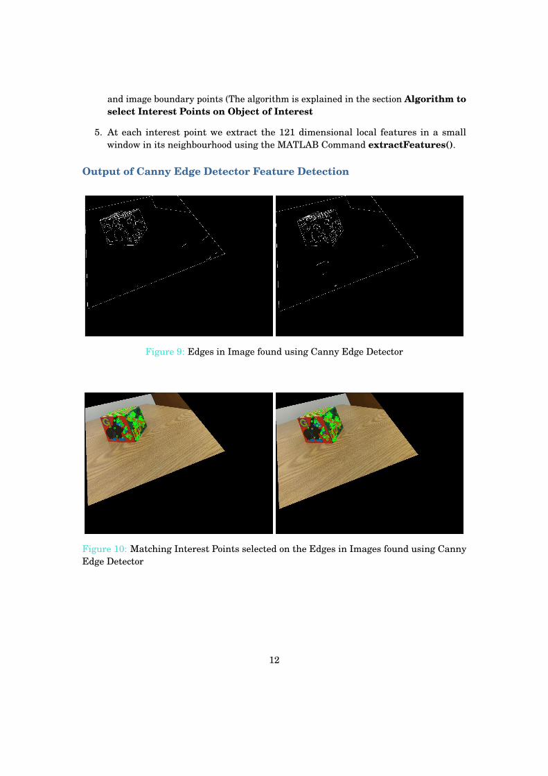
and image boundary points (The algorithm is explained in the section Algorithm toselect Interest Points on Object of Interest

5. At each interest point we extract the 121 dimensional local features in a smallwindow in its neighbourhood using the MATLAB Command extractFeatures().

Output of Canny Edge Detector Feature Detection

Figure 9: Edges in Image found using Canny Edge Detector

Figure 10: Matching Interest Points selected on the Edges in Images found using CannyEdge Detector

12

Figure 11: Matching Interest Points selected on the Edges in Image found using CannyEdge Detector

13

Finding Correspondences

After the local features from 2 stereo images are found, we need to establish correspon-dences by comparing the features or descriptors (for SIFT) between image pairs. The2 methods that are used are SSD (Sum of Squared Differences) and NCC (NormalizedCross-Correlation).These are required to compare the interest points in two images of thesame scene captured from 2 different viewpoints.The two metrics used are:

Sum of Squared Differences

After finding the features from 2 images we find SSD after summing over the featuredimensions as shown below:

SSD =∑i

∑j| f1(i, j)− f2(i, j)|2

We compute the SSD for each pair of the features and take the minimal one as thecorresponding features.

Normalised Cross-Correlation

After finding the features from 2 images we find NCC after summing over the featuredimensions as shown below:

NCC =∑

i∑

j ( f1(i, j)−m1)( f2(i, j)−m2)√∑i∑

j ( f1(i, j)−m1)2 ∑i∑

j ( f2(i, j)−m2)2

where, mi is the mean value of all the features i. The NCC has a value between −1and 1, 1 being a perfect match. We can threshold to select points that are most likely tomatch. We compute the SSD for each pair of the features and take the minimal one as thecorresponding features. The following points are followed to find correspondences :

1. The corresponding interest point of the first image is searched for within a smallnumber of adjoining rows in the second image.This is done since the image rectifica-tion is working perfectly and both the rectified images epipoles are at infinity alongthe positive x axis.

2. Since for any interest point in the first image, we might have multiple candidates inthe second image, the NCC or SSD metric is used to select the best candidate.

3. Ambiguous correspondences are removed by using the following formula

SSDI I

SSDI> τSSD

where,SSDI I is the SSD score of the second best correspondenceSSDI is the SSD score of the best correspondenceτSSD is the threshold above which the correspondence is accepted as a valid pair.

14

Algorithm to select Interest Points on Object of Interest

Motivation

The motivation to devise this algorithm is as follows:

1. The boundary of the rectified image gives unnecessary interest points when usingthe Canny Edge Detector and any other objects or even the background gives unnec-essary interest points when using the SURF Algorithm. These correspondences areirrelevant since they do not lie on the object of interest and may often lead to wrongresults and inefficient reconstruction.

2. Since we are going to triangulate these correspondence points into world pointsand since we are concerned only about the world points on the Object of Interest, Idevised this algorithm to select only those correspondences that lie on the object ofinterest.

Algorithm

The algorithm is very simple and intutive.

1. For the purpose of image rectification, the corners/outer boundary of the objectmanual correspondences were taken at the beginning. Out of those, the 7 visiblecorner points on the object are selected. Along with that another point aprroximatelyclose enough to the centroid of the object of interest is selected.

2. The distance between this center and the 7 visible corner points are computed andthe maximum dmax is stored. The threshold is set to be

τdistance = 1.1dmax

. All the interest points on the object of interest will lie within this threshold distancesince we are taking it to be a little higher than the furthest distance of a corner fromthe approximate centroid. Equivalently, it can be thought of as drawing a spherefrom this approximate centroid with a radius of τdistance = 1.1dmax and this spherewill completely surround the object of interest. Hence all points will definitely bewithin this sphere.

3. Alternatively, instead of taking another manual correspondence for the approximatecentroid separately, this algorithm can be automated by finding the largest distancebetween 2 of the bounding points and lets say that distance is Dmax and let the 2corresponding boundary points be xbp and ybp. The approximate centroid xcentroidand the farthest distance between this center and the farthest boundary point dmaxis found as

xcentroid = xbp +ybp

2dmax = Dmax

2τdistance = 1.1dmax = 0.55∗Dmax

15

4. So the distance between all the interest points and this center xcentroid is calculatedand only those interest points which follows the following condition are retained

dinterest < τdistance

Rest of the interest points are eliminated.

Results of finding Image Correspondences

All correspondences between rectified images found using SURF Algo-rithm

Figure 12: All correspondences between rectified images found using SURF Algorithm

Figure 13: All correspondences between rectified images found using SURF Algorithm andusing my algorithm to select those correspondences lying on the object of interest

16

All correspondences found using Canny Edge Detector

Figure 14: All correspondences between rectified images found using Canny Edge Detector

Figure 15: All correspondences between rectified images found using Canny Edge Detectorand using my algorithm to select those correspondences lying on the object of interest andselecting best 200 among them

17

Projective 3D Reconstruction using Triangulation and

Refining using Levenberg Marquadt Algorithm

1. The final pixel correspondences are converted to world points in world 3D. In general,if we back project two corresponding pixels from images of the same scene intotwo different rays given by P+x in world 3D, the two rays may be skew lines andmay not intersect at all. This is the reason why we need to refine the estimate forthe fundamental matrix F and also the world 3D points that are projected back tothe images for the calculation of square of the difference with the measured pixellocations.

2. To get the world 3D points Xi, we triangulate the 2D points (xi,x′i) using the linear

triangulation method. This step is also used in the nonlinear LM optimization.

(a) For each correspondence (xi,x′i) we form the matrix

A=

uPT

3 −PT1

vPT3 −PT

2u′P′T

3 −P′T1

v′P′T3 −P′T

2

(b) Our goal is to minimize ||AX|| subject to ||X|| = 1.(c) The solution of this minimization problem is given by the null vector of A.

Hence the world 3D point Xi is given by the null vector of matrix A. This isfound by finding the SVD and then taking the eigenvector corresponding to thelowest eigenvalue.

3. Using this as an initial estimate for the world points. Let, xi and x′ i be the projectedpoints in the first and the second image respectively. We use the Levenberg Marquadt(LM) Algorithm to perform the non-linear optimization to minimize the followinggeometric distance:

d2geom =∑

i

(||xi − xi||2 +||x′

i − x′ i||2)

4. All the parameters are generated as a linear matrix comprising of the 12 elements ofthe refined projection matrix of the second image P′ and then the estimated worldcoordinates in the 3 cardinal directions worldx,worldy,worldz. The cost function isminimized using the Levenberg Marquardt Algorithm to find the optimal parameters.This is implemented in cost_function.m and optimize_NLS.m.

5. After the optimization is completed we form the refined P′ from the first 12 elementsof the optimal parameters and the form the estimated world coordinates from element13 to the last element of the optimal parameters in groups of 3, where each grouphas the estimated world coordinates worldx,worldy,worldz of a correspondence.

6. Using the refined P′, the 7 boundary points are triangulated to obtain the worldpoints as implemented in triangulate_points.m.

18

3D Visual Inspection

3D Reconstruction using SURF Interest Points

The world points are plotted using the MATLAB command scatter3() in blue and theboundary corner points are plotted in green and the corresponding corners are joined by redlines corresponding to the edges of the box with the MATLAB script plot_boundary_lines.m

Figure 16: 3D Scene Reconstruction from 2 different viewpoints using SURF correspon-dences

19

Figure 17: SURF Interest points in images that is being triangulated to 3D world points

Figure 18: Point Correspondences between the images and 3D world points using SURFcorrespondences

20

3D Reconstruction using Canny Edge Detector Interest Points

The world points are plotted using the MATLAB command scatter3() in blue and theboundary corner points are plotted in green and the corresponding corners are joined by redlines corresponding to the edges of the box with the MATLAB script plot_boundary_lines.m

Figure 19: 3D Scene Reconstruction from 2 different viewpoints using Canny Edge Detectorcorrespondences

21

Figure 20: Canny Edge Detector Interest points in images that is being triangulated to 3Dworld points

Figure 21: Point Correspondences between the images and 3D world points using CannyEdge Detector correspondences

22

Improvements after optimization using Levenberg Marquadt

The improvements are enumerated below

1. The use of Levenberg Marquardt Algorithm improves the estimate of the Fundamen-tal Matrix F and Second Camera Projection Matrix P′. If it is not used, then once weenforce the rank constraint on F, everything breaks down and hence it is absolutelynecessary to do the LM Optimization.

2. I measured the Mean Square Errors before and after the LM Optimization. Theerror function includes the difference of the elements of P′ and the estimates of theWorld Points.The errors are enumerated below.

(a) Estimation of Fundamental Matrix from manual correspondences :The Mean Square Error decreased from 0.4904 to 0.1741

(b) Triangulation of SURF Correspondences to find World Points :The Mean Square Error decreased from 0.1187 to 0.0365

(c) Triangulation of Canny Edge Correspondences to find World Points :The Mean Square Error decreased from 0.0626 to 0.0299

Observations

1. Selecting the manual correspondences accurately is important for good estimateof fundamental matrix F and for image rectification. The advantage of takingmanual correspondences is that we utilise human knowledge to select the appropriatecorrespondences, but the disadvantage is that human eye is not able to detect theexact sub-pixel level correspondences.

2. The 3D scene that we reconstructed appears to be projectively distorted, since we areusing uncalibrated cameras. We estimate the fundamental matrix directly from theimages and then construct a canonical configuration for the cameras and computethe scene structure. This results in reconstruction upto a projective distortion. It ispossible to do affine and similarity restoration, based on how rich the scene is.

3. The canny edge detector gives a very large number of edge pixels. This makes theoverall reconstruction process slower as compared to the SURF.Canny edge Detectorcan give bad results if all the interest points that are chosen lie on the same edge.Then there is not much information change in the descriptors and they look thesame.In my algorithm pixels are chosen such that there is a gap of 10 interests pointsbetween those selected from all the 10000 interest points generated to eliminatethis possibility.By this I finally choose around 1000 interest points before findingcorrespondences.

4. I have used my own algorithm to choose only those interest points that lie on theobject of interest, which removes unnecessary world points (on boundaries in case of

23

Canny edge detector and on background objects in both SURF and CED) and makesthe overall 3D reconstruction process much more accurate and better. The detailedalgorithm is elaborated in the section Algorithm to select Interest points on the objectof Interest.

5. Image rectification worked very well and after rectification of the images, the cor-respondences appear on a small range of adjoining rows that are very close to eachother.

6. Levenberg Marquardt optimization improves the estimate of fundamental matrixand the world points as mentioned in the previous section.

7. The accuracy of the 3D reconstruction depends on the kind of the scene we are tryingto capture. The richer the scene is in structure, the easier it is to find interest pointsand the better results it gives.In my case, I had chosen a box object with manydrawings in it and it was visually rich. This was done for the purpose of finding bothcorners for SURF and also edges for Canny Edge Detector. I have presented thefinal 3D Reconstruction obtained from correspondences from both the Canny EdgeDetector and SURF in a similar format(configuration/orientation) for comparison.Both seem to be equally good. The difference between the 3D reconstruction modelgenerated by the SURF and Canny Edge Detector Algorithm can be observed in theworld points plotted in blue. It could be clearly mapped which interest point on theimage maps to which world point in either case.I have also presented the interestpoints chosen for both SURF and Canny Edge Detector, alongside for reference.

24

Source Code

Main Script

1

Table of Contents....................................................................................................................................... 1Load images and find manual correspondences ........................................................................ 1Estimate Fundamental Matrix and refine F using LM Optimization .............................................. 1Rectify Images ................................................................................................................... 2Manually select the boundary points of the object of interest ...................................................... 2Manually select the approximate center of the object of interest .................................................. 3Remove the world points that do not belong to the object of interest ............................................ 3Detect Features using SURF and find correspondences in rectified image ...................................... 3Implementation 1 ................................................................................................................ 3Implementation 2 ................................................................................................................ 4Triangulate the SURF Correspondences into World 3D Points .................................................... 4Traingulate boundary points and plot world points on object of interest ........................................ 4Detect Features using CED and find correspondences in rectified image ....................................... 4Implementation 1 ................................................................................................................ 4Implementation 2 ................................................................................................................ 5Triangulate the Canny Edge Detector Correspondences into World 3D Points ................................ 5Triangulate boundary points and plot world points on object of interest ........................................ 5

%%%%%%%%%%%%%%%%%%%%%%%%%%%%%%%%%%%%%%%%%%%%%%%%%%%%%%%%%%%%%%%%%%%%%%%%%%%% This is the main script for running the program for 3D Reconstruction% Author : Rohan Sarkar%%%%%%%%%%%%%%%%%%%%%%%%%%%%%%%%%%%%%%%%%%%%%%%%%%%%%%%%%%%%%%%%%%%%%%%%%%%

Load images and find manual correspon-dences

clc; close all; clear;image1 = imread('7.jpg');image2 = imread('8.jpg');find_manual_correspondence;figure,showMatchedFeatures(image1, image2, x1(:,1:2), x2(:,1:2),'montage');title('Showing all selected correspondences');

Estimate Fundamental Matrix and refine F us-ing LM Optimization

Load manual correspondences

clc; close all; clear;image1 = imread('7.jpg');image2 = imread('8.jpg');load 'correspondences78.mat';% Converting the physical pixel coordinates to homogeneous coordinatesx1 = [mc_image1 ones(size(mc_image1,1),1)];x2 = [mc_image2 ones(size(mc_image1,1),1)];% Find Transformation to normalize the manual correspondencesT1 = find_transformation_to_normalize(x1);

25

2

T2 = find_transformation_to_normalize(x2);% Estimate the Fundamental Matrix using Linear Least Squares Method and% enforce the rank constraint by conditioning the Fundamental MatrixF = estimate_Fundamental_Matrix(x1,x2,T1,T2);F = F/F(3,3);% Find the epipoles of the 2 cameras% Find the epipole of the first camera as the right null vector of Fe1 = null(F);e1 = e1/e1(3);% Find the epipole of the first camera as the left null vector of Fe2 = null(F');e2 = e2/e2(3);% Finding the cross product form of the epipole of the second camerae2_cross = [0 -e2(3) e2(2);e2(3) 0 -e2(1);-e2(2) e2(1) 0];% Finding the Projection MatrixP1 = [eye(3), zeros(3,1)];P2 = [e2_cross*F,e2];[P2_refine, F_refine, X_world] = optimize_NLS(@cost_function,x1,x2,P1,P2);F_refine = F_refine/F_refine(3,3);% Find the epipole of the first camera as the right null vector of Fe1_refine = null(F_refine);e1_refine = e1_refine/e1_refine(3);% Find the epipole of the first camera as the left null vector of Fe2_refine = null(F_refine');e2_refine = e2_refine/e2_refine(3);

Rectify ImagesFind the rectification Homographies for both images

[x1_rectified, x2_rectified, H1, H2, F_rectified, ... e1_rectified, e2_rectified] = find_rectification_homographies... (image1,image2,x1,x2,e1_refine,e2_refine,F_refine,P1,P2_refine)% Apply the rectification Homographies with appropriate scaling and% shifting to rectify both images[image1_rectified, H1_rectified, xH1] = rectify_images (image1,H1,x1);[image2_rectified, H2_rectified, xH2] = rectify_images (image2,H2,x2);% Display the rectified imagesfigureimshow(image1_rectified)figureimshow(image2_rectified)% Display the manual correspondences between the rectified imagesfigure, showMatchedFeatures(image1_rectified, image2_rectified,... xH1(:,1:2), xH2(:,1:2), 'montage');title('Showing all rectified manual correspondences');

Manually select the boundary points of the ob-ject of interest

figure1 = imshow(image1_rectified,'InitialMagnification', 300);xir1=ginput;

26

3

% Count number of correspondences selectedn = size(xir1,1);close all;% display image and get the correspondence points for the second imagefigure2 = imshow(image2_rectified,'InitialMagnification', 300);xir2=ginput(n);close all;figure,showMatchedFeatures(image1,image2,xir1(:,1:2),xir2(:,1:2),'montage');title('Showing all selected correspondences');

Manually select the approximate center of theobject of interest

figure1 = imshow(image1_rectified,'InitialMagnification', 300);xirc1=ginput(1);close all;% display image and get the correspondence points for the second imagefigure2 = imshow(image2_rectified,'InitialMagnification', 300);xirc2=ginput(1);close all;save('bp7.mat','xir1','xir2','xirc1','xirc2');

Remove the world points that do not belong tothe object of interest

Calculate the maximum distance of boundary points from the center which will be the threshold for elim-inating unnecesssary points that do not belong to the object of interest

load('bp7.mat');difference = xir1-repmat(xirc1,size(xir1,1),1);distance = sqrt(difference(:,1).^2+difference(:,2).^2)threshold_distance1 = 1.1*max(distance);difference = xir2-repmat(xirc2,size(xir2,1),1);distance = sqrt(difference(:,1).^2+difference(:,2).^2)threshold_distance2 = 1.1*max(distance);

Detect Features using SURF and find corre-spondences in rectified image

Detect SURF Features and the interest points

[SURF_features1,SURF_interest_points1]=find_SURF_features(image1_rectified);[SURF_features2,SURF_interest_points2]=find_SURF_features(image2_rectified);% Find correspondence between the interest points in the two rectified% images using SSD

Implementation 1[x1_SURF,x2_SURF] = detect_correspondences(image1_rectified, ...

27

4

image2_rectified,SURF_features1,SURF_features2,... SURF_interest_points1.Location,SURF_interest_points2.Location,... 0.7,5,xirc1,threshold_distance1);

Implementation 2[x1_SURF,x2_SURF] = detect_correspondences_SSD(image1_rectified,... image2_rectified,SURF_features1,SURF_features2,... SURF_interest_points1,SURF_interest_points2,xirc1, threshold_distance1);

Triangulate the SURF Correspondences intoWorld 3D Points

[P1_SURF,P2_refine_SURF, F_refine_SURF, X_world_SURF] = ... triangulate_world_points(x1_SURF,x2_SURF);

Traingulate boundary points and plot worldpoints on object of interest

Triangulate the boundary points into World 3D points

[X_bound_OI] = triangulate_points(xir1,xir2,P1_SURF,P2_refine_SURF);% Plot World 3D points of the SURF Interest Pointsscatter3(X_world_SURF(:,1),X_world_SURF(:,2),X_world_SURF(:,3),... 'MarkerEdgeColor','k','MarkerFaceColor','b');hold on;% Plot the boundary and edgesscatter3(X_bound_OI(:,1),X_bound_OI(:,2),X_bound_OI(:,3),... 'MarkerEdgeColor','k','MarkerFaceColor','g');plot_boundary_lines;hold off;

Detect Features using CED and find correspon-dences in rectified image

Detect Canny Edge Detector Features and the interest points

[CED_features1, CED_interest_points1] = find_CED_features... (image1_rectified,0.2,xirc1,threshold_distance1);[CED_features2, CED_interest_points2] = find_CED_features... (image2_rectified,0.2,xirc2,threshold_distance2);% Find correspondence between the interest points in the two rectified% images using SSD

Implementation 1[x1_CED,x2_CED] = detect_correspondences(image1_rectified, ...

28

5

image2_rectified,CED_features1,CED_features2,CED_interest_points1,... CED_interest_points2,0.7,5,xirc1,threshold_distance1);

Implementation 2[x1_CED,x2_CED] = find_correspondences(image1_rectified,... image2_rectified,CED_features1,CED_features2,CED_interest_points1,... CED_interest_points2);

Triangulate the Canny Edge Detector Corre-spondences into World 3D Points

[P1_CED,P2_refine_CED, F_refine_CED, X_world_CED] = ... triangulate_world_points(x1_CED,x2_CED);

Triangulate boundary points and plot worldpoints on object of interest

Triangulate the boundary points into World 3D points

[X_bound_OI] = triangulate_points(xir1,xir2,P1_CED,P2_refine_CED);% Plot World 3D points of the Canny Edge Detector Interest Pointsscatter3(X_world_CED(:,1),X_world_CED(:,2),X_world_CED(:,3),... 'MarkerEdgeColor','k','MarkerFaceColor','b');hold on;% Plot World 3D points of boundary points and the edgesscatter3(X_bound_OI(:,1),X_bound_OI(:,2),X_bound_OI(:,3),... 'MarkerEdgeColor','k','MarkerFaceColor','g');plot_boundary_lines;hold off;

Published with MATLAB® R2013a

29

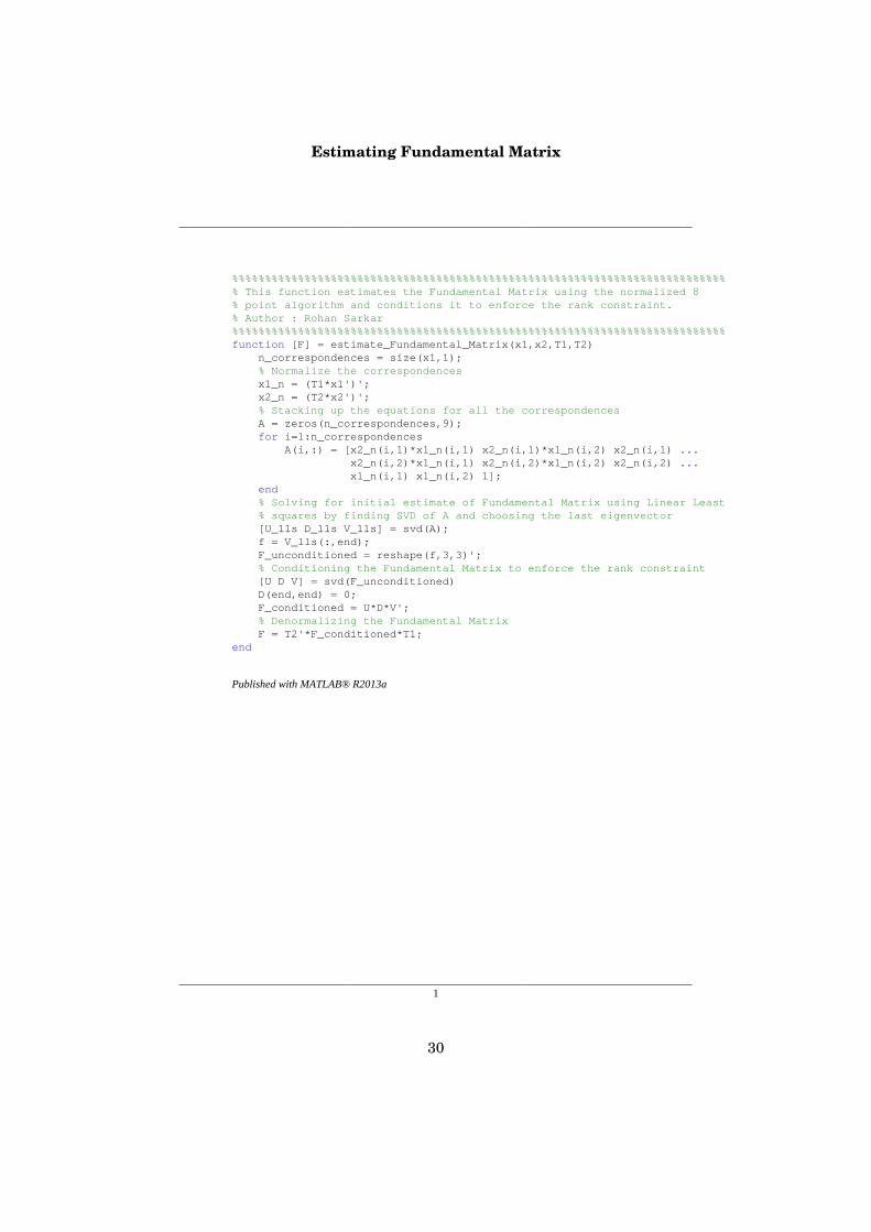
Estimating Fundamental Matrix

1

%%%%%%%%%%%%%%%%%%%%%%%%%%%%%%%%%%%%%%%%%%%%%%%%%%%%%%%%%%%%%%%%%%%%%%%%%%%% This function estimates the Fundamental Matrix using the normalized 8% point algorithm and conditions it to enforce the rank constraint.% Author : Rohan Sarkar%%%%%%%%%%%%%%%%%%%%%%%%%%%%%%%%%%%%%%%%%%%%%%%%%%%%%%%%%%%%%%%%%%%%%%%%%%%function [F] = estimate_Fundamental_Matrix(x1,x2,T1,T2) n_correspondences = size(x1,1); % Normalize the correspondences x1_n = (T1*x1')'; x2_n = (T2*x2')'; % Stacking up the equations for all the correspondences A = zeros(n_correspondences,9); for i=1:n_correspondences A(i,:) = [x2_n(i,1)*x1_n(i,1) x2_n(i,1)*x1_n(i,2) x2_n(i,1) ... x2_n(i,2)*x1_n(i,1) x2_n(i,2)*x1_n(i,2) x2_n(i,2) ... x1_n(i,1) x1_n(i,2) 1]; end % Solving for initial estimate of Fundamental Matrix using Linear Least % squares by finding SVD of A and choosing the last eigenvector [U_lls D_lls V_lls] = svd(A); f = V_lls(:,end); F_unconditioned = reshape(f,3,3)'; % Conditioning the Fundamental Matrix to enforce the rank constraint [U D V] = svd(F_unconditioned) D(end,end) = 0; F_conditioned = U*D*V'; % Denormalizing the Fundamental Matrix F = T2'*F_conditioned*T1;end


30

Optimize using Levenberg Marquardt Method

1

%%%%%%%%%%%%%%%%%%%%%%%%%%%%%%%%%%%%%%%%%%%%%%%%%%%%%%%%%%%%%%%%%%%%%%%%%%%% This function is used to refine the parameters and also triangulate image% pixel correspondences generated by the SURF and Canny Edge Detector to% world 3D points% Author : Rohan Sarkar%%%%%%%%%%%%%%%%%%%%%%%%%%%%%%%%%%%%%%%%%%%%%%%%%%%%%%%%%%%%%%%%%%%%%%%%%%%function [P2_refine F_refine X_world] = optimize_NLS... (cost_function, x1, x2, P1, P2) % Unroll the P2 matrix and add it to first 12 elements of parameters p = P2'; parameters = p(:)'; n_correspondences = size(x1,1); % Triangulate the correspondence to the world 3D points and add the % estimates as parameters vector X_world = zeros(n_correspondences,3); for i = 1:n_correspondences A = find_A(P1,P2,x1(i,:),x2(i,:)); [U,D,V] = svd(A); x_w = V(:,end); x_w = x_w./x_w(4); X_wn = [x_w(1) x_w(2) x_w(3)]; parameters = [parameters X_wn]; end % Applying the Levenberg Marquardt algorithm to find the optimal % parameters and refine the estimates of the world 3D points options = optimoptions('lsqnonlin','Algorithm','levenberg-marquardt'... ,'TolX',0.00000000001,'TolFun',0.00000000001); optimal_parameters = lsqnonlin(cost_function,parameters,[],[],... options,x1,x2); % Regenerate the refined camera projection matrix from the optimal % parameters P2_refine = reshape(optimal_parameters(1:12),4,3)'; t = P2_refine(:,4); e_cross = [0 -t(3) t(2); t(3) 0 -t(1); -t(2) t(1) 0]; M = P2_refine(:,1:3); % Find the refined fundamental matrix from the optimal parameters F_refine = e_cross*M; % Regenerate the estimates of world points from the optimal parameters X_world = reshape(optimal_parameters(13:end),3,n_correspondences)'; error_before_refine = cost_function(parameters,x1, x2)'; % Find the mean square error before applying LM Optimization ms_error_before_refine = mean(error_before_refine.^2) % Find the mean square error after applying LM Optimization error_after_refine = cost_function(optimal_parameters,x1, x2)'; ms_error_after_refine = mean(error_after_refine.^2)end


31

Rectification of images by applying Homography

1

%%%%%%%%%%%%%%%%%%%%%%%%%%%%%%%%%%%%%%%%%%%%%%%%%%%%%%%%%%%%%%%%%%%%%%%%%%%% This function is used to rectify the images by applying the Rectification% Homographies generated in function find_rectification_homographies% Author : Rohan Sarkar%%%%%%%%%%%%%%%%%%%%%%%%%%%%%%%%%%%%%%%%%%%%%%%%%%%%%%%%%%%%%%%%%%%%%%%%%%%function [image_rectified, H_rectified, xH] = rectify_images (image,H,x) % Computing dimensions and boundary points of image height_original = size(image,1);width_original = size(image,2); image = single(image); bp(:,1) = [1;1;1]; bp(:,2) = [width_original;1;1]; bp(:,3) = [1;height_original;1]; bp(:,4) = [width_original;height_original;1]; % Apply the rectification Homography to compute where the original % boundary is mapped in the rectified image bpr = H*bp; for i =1:4 bpr(:,i) = bpr(:,i)/bpr(3,i); bpr(:,i) = bpr(:,i)/bpr(3,i); end bpr = round(bpr)'; % Find the minimum and maximum coordinates to calculate the height and % width of the rectified image t_min = min(bpr); t_max = max(bpr); height_projected = t_max(2)-t_min(2); width_projected = t_max(1)-t_min(1); % Scaling the image to preserve the original aspect ratio H_scale = [width_original/width_projected 0 0; 0 height_original/height_projected 0; 0 0 1]; % Compute the new Homography after scaling the image and applying this % new Homography to the original points H = H_scale*H; bpr = H*bp; for i =1:4 bpr(:,i) = bpr(:,i)/bpr(3,i); bpr(:,i) = bpr(:,i)/bpr(3,i); end bpr = round(bpr)'; % Finding the offsets in x and y axes t_min = min(bpr); offset_x = t_min(1); offset_y = t_min(2); % Shifting the image by the offset T = [1 0 -offset_x+1; 0 1 -offset_y+1;0 0 1]; % Computing the new Homography for rectifying the image H_rectified = T*H; H_rect_inv = pinv(H_rectified); image_rectified = zeros(height_original,width_original,3); % Apply the computed rectification homography after scaling and % shifting to the original image to get the rectified image

32

2

for i = 1:height_original for j = 1:width_original point = H_rect_inv*[i;j;1]; point = point/point(3); % Checking if the point generated lies within the original % image and then applying bilinear interpolation to get the % corresponding RGB Value at that pixel if (point(1)>1 && point(1)<height_original &&... point(2)>1 && point(2)<width_original) image_rectified(i,j,:) = bilinear_interpolation... (image,[point(1);point(2)],0.00001); end end end % Find all the rectified manual points image_rectified = uint8(image_rectified); xH = (H_rectified*x')'; for i =1:size(xH,1) xH(i,:) = xH(i,:)/xH(i,3); endend


33

Cost Function for LM Optimization

1

%%%%%%%%%%%%%%%%%%%%%%%%%%%%%%%%%%%%%%%%%%%%%%%%%%%%%%%%%%%%%%%%%%%%%%%%%%%% This function is the cost function used for the Levenberg Marquadt% Optimization to refine the parameters and also to triangulate% correspondence to World 3D for 3D Reconstruction% Author : Rohan Sarkar%%%%%%%%%%%%%%%%%%%%%%%%%%%%%%%%%%%%%%%%%%%%%%%%%%%%%%%%%%%%%%%%%%%%%%%%%%%function error = cost_function(parameters,xref1, xref2) n_correspondences = size(xref1,1); % Retrieve the Projection Matrices from Parameters P1 = [eye(3), zeros(3,1)]; P2 = reshape(parameters(1:12),4,3)'; % Retrieve the estimated World Points from Parameters X_world = reshape(parameters(13:end),3,n_correspondences)'; X_world = [X_world, ones(n_correspondences,1)]; % Project the world points onto the two images and find pixel % coordinates xp1 = P1*X_world'; xp2 = P2*X_world'; for i =1:n_correspondences xp1(:,i) = xp1(:,i)/xp1(3,i); xp2(:,i) = xp2(:,i)/xp2(3,i); end % unroll all the pixel coordinates xp1 = xp1';xp1 = xp1(:,1:2); xp2 = xp2';xp2 = xp2(:,1:2); % Find the error function between the actual points and the projected % points in both the images and concatenate them to form the error % function error1 = xp1 - xref1(:,1:2); error2 = xp2 - xref2(:,1:2); error1 = error1';error1 = error1(:)'; error2 = error2';error2 = error2(:)'; error = [error1 error2];end


34

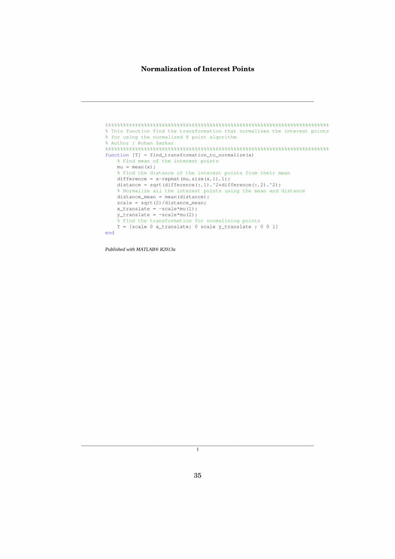
Normalization of Interest Points

1

%%%%%%%%%%%%%%%%%%%%%%%%%%%%%%%%%%%%%%%%%%%%%%%%%%%%%%%%%%%%%%%%%%%%%%%%%%%% This function find the transformation that normalizes the interest points% for using the normalized 8 point algorithm% Author : Rohan Sarkar%%%%%%%%%%%%%%%%%%%%%%%%%%%%%%%%%%%%%%%%%%%%%%%%%%%%%%%%%%%%%%%%%%%%%%%%%%%function [T] = find_transformation_to_normalize(x) % Find mean of the interest points mu = mean(x); % Find the distance of the interest points from their mean difference = x-repmat(mu,size(x,1),1); distance = sqrt(difference(:,1).^2+difference(:,2).^2); % Normalize all the interest points using the mean and distance distance_mean = mean(distance); scale = sqrt(2)/distance_mean; x_translate = -scale*mu(1); y_translate = -scale*mu(2); % Find the transformation for normalizing points T = [scale 0 x_translate; 0 scale y_translate ; 0 0 1]end


35

Finding Rectification Homographies

1

%%%%%%%%%%%%%%%%%%%%%%%%%%%%%%%%%%%%%%%%%%%%%%%%%%%%%%%%%%%%%%%%%%%%%%%%%%%% This function finds the homographies for rectification of the two images% Author : Rohan Sarkar%%%%%%%%%%%%%%%%%%%%%%%%%%%%%%%%%%%%%%%%%%%%%%%%%%%%%%%%%%%%%%%%%%%%%%%%%%%function [x1_rectified, x2_rectified, H1, H2, F_rectified,... e1_rectified,e2_rectified] = ... find_rectification_homographies(image1,image2,x1,x2,e1,e2,F,P1,P2) % Find the dimensions of the images height = size(image1,1); width = size(image1,2); % Find the number of manual correspondences n_correspondences = size(x1,1); % Find angle of epipole w.r.t x axis for rotating image angle = atan(-(e2(2)-height/2)/(e2(1)-width/2)); f = cos(angle)*(e2(1)-width/2)-sin(angle)*(e2(2)-height/2); G = [1 0 0;0 1 0;-1/f 0 1]; % Rotation Matrix to rotate the image so that epipole goes to x axis R = [cos(angle) -sin(angle) 0;sin(angle) cos(angle) 0; 0 0 1]; % Homography to translate the second image center to origin T = [1 0 -width/2;0 1 -height/2;0 0 1]; H2 = G*R*T; image_center = [width/2;height/2;1]; center_rectified = H2*image_center; center_rectified = center_rectified/center_rectified(3); % Homography to translate second image center back to original center T2 = [1 0 width/2-center_rectified(1); 0 1 height/2-center_rectified(2); 0 0 1]; % Overall Homography for rectification of second image H2 = T2*H2; % Finding the overall Homography for rectification of first image % as described in textbook % Find M M = P2*pinv(P1); % Find H0 H0 = H2*M; % Project the manual correspondences and find pixel coordinates x1_hat = (H0*x1')'; x2_hat = (H2*x2')'; for i =1:n_correspondences x1_hat(i,:) = x1_hat(i,:)/x1_hat(i,3); x2_hat(i,:) = x2_hat(i,:)/x2_hat(i,3); end % Solve for a,b,c for H_A using Linear Least Squares that minimizes % function A = x1_hat; b = x2_hat(:,1); x = pinv(A)*b; HA = [x(1) x(2) x(3); 0 1 0; 0 0 1]; H1 = HA*H0; center_rectified = H1*image_center; center_rectified = center_rectified/center_rectified(3); % Homography to translate first image center back to original center

36

2

T1 = [1 0 width/2-center_rectified(1); 0 1 height/2-center_rectified(2); 0 0 1]; % Overall Homography for rectification of first image H1 = T1*H1; F_rectified = inv(H2')*F*inv(H1); % Find the pixel coordinates rectified manually selected points x1_rectified = (H1*x1')'; x2_rectified = (H2*x2')'; for i =1:n_correspondences x1_rectified(i,:) = x1_rectified(i,:)/x1_rectified(i,3); x2_rectified(i,:) = x2_rectified(i,:)/x2_rectified(i,3); end % Find the epipole of the first camera as the right null vector of F e1_rectified = null(F_rectified); e1_rectified = e1_rectified/e1_rectified(3); % Find the epipole of the second camera as the left null vector of F e2_rectified = null(F_rectified'); e2_rectified = e2_rectified/e2_rectified(3);end


37

Finding SURF Features and interest points

1

%%%%%%%%%%%%%%%%%%%%%%%%%%%%%%%%%%%%%%%%%%%%%%%%%%%%%%%%%%%%%%%%%%%%%%%%%%%% This function finds the SURF Features and the valid interest points% Author : Rohan Sarkar%%%%%%%%%%%%%%%%%%%%%%%%%%%%%%%%%%%%%%%%%%%%%%%%%%%%%%%%%%%%%%%%%%%%%%%%%%%function [ref_features, ref_valid_points] = find_SURF_features(ref_image) % Convert RGB to Gray scale image ref_image_gray = rgb2gray(ref_image); % Detect SURF Features ref_points = detectSURFFeatures(ref_image_gray); % Select the best 200 Features among them ref_points = ref_points.selectStrongest(200); % Extract the corresponding features and the valid interest points [ref_features, ref_valid_points] = extractFeatures(ref_image_gray,... ref_points); % Display the features figure; imshow(ref_image); hold on; plot(ref_points.selectStrongest(200)); hold off; % Display the best 40 Visual SURF features figure; subplot(5,8,3); title('Best 40 Features'); for i=1:40 scale = ref_points(i).Scale; image = imcrop(ref_image,[ref_points(i).Location-10*scale ... 20*scale 20*scale]); subplot(5,8,i); imshow(image); hold on; rectangle('Position',[5*scale 5*scale 10*scale 10*scale],... 'Curvature',1,'EdgeColor','g'); end hold off;end


38

Finding Canny Edge Detector Features and interest points

1

%%%%%%%%%%%%%%%%%%%%%%%%%%%%%%%%%%%%%%%%%%%%%%%%%%%%%%%%%%%%%%%%%%%%%%%%%%%% This function finds the Canny Edge Detector Features and the% valid interest points on the edges detected% Author : Rohan Sarkar%%%%%%%%%%%%%%%%%%%%%%%%%%%%%%%%%%%%%%%%%%%%%%%%%%%%%%%%%%%%%%%%%%%%%%%%%%%function [CED_features, CED_interest_points] = find_CED_features... (image, canny_threshold,xirc,distance_threshold) % Convert to gray scale image imagec = rgb2gray(image); % Find the edges in the image using Canny Edge Detector edgec = edge(imagec,'canny',canny_threshold); % Display edges figure imshow(edgec); % Find the interest points by pointing out the 1s in the images which % signify the edges [row,col,v] = find(edgec); % Put the interest point in (x,y) format ipc = [col row]; % Use own algorithm (described in report) to choose only points on the % object of interest by eliminating those points which lie outside the % maximum distance threshold from the center of the object of interest difference = ipc-repmat(xirc,size(ipc,1),1); distance = sqrt(difference(:,1).^2+difference(:,2).^2); index = find(distance < distance_threshold); ipc = ipc(index,:); % Since this gives plenty of interest points, points are chosen with a % uniform gap so that consecutive points on the same edge are not % chosen for better and accurate results index = 1000:10:size(ipc,1); ip_ced = ipc(index,:); % Extract the 121 dimensional Canny Edge Detector Feature Vector in a % local windoe around the interest points detected [CED_features, CED_interest_points] = extractFeatures(imagec,ip_ced);end


39

Correspondence detection using SSD (Implementation 1)

1

%%%%%%%%%%%%%%%%%%%%%%%%%%%%%%%%%%%%%%%%%%%%%%%%%%%%%%%%%%%%%%%%%%%%%%%%%%%% This function is used to find the correspondences between the interest% points generated using SURF or Canny Edge Detector between the rectified% images using SSD% Author : Rohan Sarkar%%%%%%%%%%%%%%%%%%%%%%%%%%%%%%%%%%%%%%%%%%%%%%%%%%%%%%%%%%%%%%%%%%%%%%%%%%%function [x1_c,x2_c] = detect_correspondences(rect_image1, rect_image2,... f1,f2,x1,x2,local_t,global_t,xirc1,threshold) x1_c = [];x2_c = []; % Establishing the SSD Metric SSD_metric = zeros(size(x1,1),size(x2,1)); for i = 1:size(x1,1) for j = 1:size(x2,1) SSD_metric(i,j) = sum((f1(i,:)-f2(j,:)).^2); end end % Find the global mean global_mu = mean(SSD_metric(:)); for i = 1:size(x1,1) % Finding mean for a particular row or a correspondence min1 = min(SSD_metric(i,:)); % Checking if it fulfils the global criterion for being a suitable % correspondence if (min1 <= global_t*global_mu) % Replace the best minimum with inf to find second best minimum [~,id] = min(SSD_metric(i,:)); SSD_metric(i,id) = inf; % Find second minimum min2 = min(SSD_metric(i,:)); % Check if it fulfils the local criterion for being a suitable % correspondence if(min1/min2<local_t) x1_c = [x1_c;x1(i,:)]; x2_c = [x2_c;x2(id,:)]; SSD_metric(:,id) = inf; end else continue; end end % Since image rectification is working we seach for nearby 50 rows of % the image and search for the correspondences only among these 50 % adjoining rows [index, val] = find(abs(x1_c(:,2)-x2_c(:,2))<50); x1_c = x1_c(index,:); x2_c = x2_c(index,:); % Use own algorithm (described in report) to choose only correspondence % on the object of interest by eliminating those points which lie % outside the maximum distance threshold from the center of the object % of interest difference = x1_c(:,1:2)-repmat(xirc1,size(x1_c,1),1); distance = sqrt(difference(:,1).^2+difference(:,2).^2);

40

2

index = find(distance<threshold); x1_c = x1_c(index,:); x2_c = x2_c(index,:); % Plot the correspondences between rectified images figure, showMatchedFeatures(rect_image1, rect_image2, ... x1_c, x2_c, 'montage'); title('Showing all matches');end


41

Correspondence detection using SSD (Implementation 2)

1

%%%%%%%%%%%%%%%%%%%%%%%%%%%%%%%%%%%%%%%%%%%%%%%%%%%%%%%%%%%%%%%%%%%%%%%%%%%% This function is used to find the correspondences between the interest% points generated using SURF or Canny Edge Detector between the rectified% images using SSD% Author : Rohan Sarkar%%%%%%%%%%%%%%%%%%%%%%%%%%%%%%%%%%%%%%%%%%%%%%%%%%%%%%%%%%%%%%%%%%%%%%%%%%%function [x1,x2] = detect_correspondences_SSD(rect_image1,... rect_image2,features1,features2,interest_points1,interest_points2,... xirc1,threshold)% Establishing the SSD Metricindex_pairs = matchFeatures(features1, features2,'Metric','SSD');[val,index] = unique(index_pairs(:,2));index_pairs = index_pairs(index,:);x1 = interest_points1(index_pairs(:,1)).Location;x2 = interest_points2(index_pairs(:,2)).Location;% Since image rectification is working we seach for nearby 50 rows of the% image and search for the correspondences only among these 50 adjoining% rows[index, val] = find(abs(x1(:,2)-x2(:,2))<50);x1 = x1(index,:);x2 = x2(index,:);% Use own algorithm (described in report) to choose only correspondences on% the object of interest by eliminating those points which lie outside the% maximum distance threshold from the center of the object of interestdifference = x1(:,1:2)-repmat(xirc1,size(x1,1),1);distance = sqrt(difference(:,1).^2+difference(:,2).^2);index = find(distance<threshold);x1 = x1(index,:);x2 = x2(index,:);% Displaying the matched featuresfigure, showMatchedFeatures(rect_image1, rect_image2, ... x1, x2, 'montage');title('Showing all matches');


42

Triangulate World Points for 3D Reconstruction

1

%%%%%%%%%%%%%%%%%%%%%%%%%%%%%%%%%%%%%%%%%%%%%%%%%%%%%%%%%%%%%%%%%%%%%%%%%%%% This function is used to triangulate the detected correspondences in SURF% and Canny Edge Detector into the world 3D points for 3D reconstruction% Author : Rohan Sarkar%%%%%%%%%%%%%%%%%%%%%%%%%%%%%%%%%%%%%%%%%%%%%%%%%%%%%%%%%%%%%%%%%%%%%%%%%%%function [P1,P2_refine, F_refine, X_world] = triangulate_world_points(x1,x2)x1 = double([x1(:,1),x1(:,2),ones(size(x1,1),1)]);x2 = double([x2(:,1),x2(:,2),ones(size(x2,1),1)]);% Find Transformation to normalize the manual correspondencesT1 = find_transformation_to_normalize(x1);T2 = find_transformation_to_normalize(x2);% Estimate the Fundamental Matrix using Linear Least Squares Method and% enforce the rank constraint by conditioning the Fundamental MatrixF = estimate_Fundamental_Matrix(x1,x2,T1,T2);F = F/F(3,3);% Find the epipoles of the 2 cameras% Find the epipole of the first camera as the right null vector of Fe1 = null(F);e1 = e1/e1(3);% Find the epipole of the first camera as the left null vector of Fe2 = null(F');e2 = e2/e2(3);% Finding the cross product form of the epipole of the second camerae2_cross = [0 -e2(3) e2(2);e2(3) 0 -e2(1);-e2(2) e2(1) 0];% Finding the Projection MatrixP1 = [eye(3), zeros(3,1)];P2 = [e2_cross*F,e2];[P2_refine, F_refine, X_world] = optimize_NLS(@cost_function, x1, x2, P1, P2);F_refine = F_refine/F_refine(3,3);% Find the epipole of the first camera as the right null vector of Fe1_refine = null(F_refine);e1_refine = e1_refine/e1_refine(3);% Find the epipole of the first camera as the left null vector of Fe2_refine = null(F_refine');e2_refine = e2_refine/e2_refine(3);end


43

Triangulate Boundary Points for 3D Reconstruction

1

%%%%%%%%%%%%%%%%%%%%%%%%%%%%%%%%%%%%%%%%%%%%%%%%%%%%%%%%%%%%%%%%%%%%%%%%%%%% This function is used to triangulate the boundary points into the world% 3D points for marking the boundary of the object of interest during the% process of 3D reconstruction% Author : Rohan Sarkar%%%%%%%%%%%%%%%%%%%%%%%%%%%%%%%%%%%%%%%%%%%%%%%%%%%%%%%%%%%%%%%%%%%%%%%%%%%function [X_world] = triangulate_points(xir1,xir2,P1,P2) % The manually selected boundary points are first converted to % homogeneous coordinates n = size(xir1,1); xir1h = [xir1,ones(n,1)]; xir2h = [xir2,ones(n,1)]; X_world = zeros(n,3); % The boundary points are triangulated with the refined camera % projection matrices and the corresponding world 3D coordinates are % generated for i = 1:n A = find_A(P1,P2,xir1h(i,:),xir2h(i,:)); [U,D,V] = svd(A); x_w = V(:,end); x_w = x_w./x_w(4); X_world(i,:) = [x_w(1) x_w(2) x_w(3)]; endend


44

Plot Edges between Boundary Points for 3D Reconstruction

1

%%%%%%%%%%%%%%%%%%%%%%%%%%%%%%%%%%%%%%%%%%%%%%%%%%%%%%%%%%%%%%%%%%%%%%%%%%%% This script is used to draw the edges of the box in the 3D Reconstruction% between the boundary points% Author : Rohan Sarkar%%%%%%%%%%%%%%%%%%%%%%%%%%%%%%%%%%%%%%%%%%%%%%%%%%%%%%%%%%%%%%%%%%%%%%%%%%%bpl = [X_bound_OI(1,:);X_bound_OI(2,:)]plot3(bpl(:,1),bpl(:,2),bpl(:,3),'r-','Linewidth',3);bpl = [X_bound_OI(1,:);X_bound_OI(4,:)]plot3(bpl(:,1),bpl(:,2),bpl(:,3),'r-','Linewidth',3);bpl = [X_bound_OI(1,:);X_bound_OI(5,:)]plot3(bpl(:,1),bpl(:,2),bpl(:,3),'r-','Linewidth',3);bpl = [X_bound_OI(2,:);X_bound_OI(3,:)]plot3(bpl(:,1),bpl(:,2),bpl(:,3),'r-','Linewidth',3);bpl = [X_bound_OI(3,:);X_bound_OI(4,:)]plot3(bpl(:,1),bpl(:,2),bpl(:,3),'r-','Linewidth',3);bpl = [X_bound_OI(4,:);X_bound_OI(6,:)]plot3(bpl(:,1),bpl(:,2),bpl(:,3),'r-','Linewidth',3);bpl = [X_bound_OI(5,:);X_bound_OI(6,:)]plot3(bpl(:,1),bpl(:,2),bpl(:,3),'r-','Linewidth',3);bpl = [X_bound_OI(3,:);X_bound_OI(7,:)]plot3(bpl(:,1),bpl(:,2),bpl(:,3),'r-','Linewidth',3);bpl = [X_bound_OI(6,:);X_bound_OI(7,:)]plot3(bpl(:,1),bpl(:,2),bpl(:,3),'r-','Linewidth',3);


45

Selecting Manual Correspondences

1

%%%%%%%%%%%%%%%%%%%%%%%%%%%%%%%%%%%%%%%%%%%%%%%%%%%%%%%%%%%%%%%%%%%%%%%%%%%% This script is for manually selecting and recording the correspondences% between the images by clicking on the corresponding pixels directly on% the image. (The cross hair allows easy selection of the points)% Author : Rohan Sarkar%%%%%%%%%%%%%%%%%%%%%%%%%%%%%%%%%%%%%%%%%%%%%%%%%%%%%%%%%%%%%%%%%%%%%%%%%%%% display image and get the correspondence points for the first imagefigure1 = imshow(image1,'InitialMagnification', 300, 'Border','tight');mc_image1=ginput;% Count number of correspondences selectednc_image1 = size(mc_image1,1);close all;% display image and get the correspondence points for the second imagefigure2 = imshow(image2,'InitialMagnification', 300, 'Border','tight');mc_image2=ginput(nc_image1);close all;% display the correspondences manually selectedsubplot(1,2,1)imshow(image1, 'Border','tight');hold onplot(mc_image1(:,1),mc_image1(:,2),'b.', 'MarkerSize', 15);title('First Image Correspondences')hold offsubplot(1,2,2)imshow(image2, 'Border','tight');hold onplot(mc_image2(:,1),mc_image2(:,2),'r.', 'MarkerSize', 15);title('Second Image Correspondences')hold offsave 'correspondences78.mat';


46

Find A for Triangulation

1

%%%%%%%%%%%%%%%%%%%%%%%%%%%%%%%%%%%%%%%%%%%%%%%%%%%%%%%%%%%%%%%%%%%%%%%%%%%% This function is used for stacking up the eauations for triangulation of% image pixel coordinates to world 3D for 3D Reconstruction% Author : Rohan Sarkar%%%%%%%%%%%%%%%%%%%%%%%%%%%%%%%%%%%%%%%%%%%%%%%%%%%%%%%%%%%%%%%%%%%%%%%%%%%function [A] = find_A (P1,P2,x1,x2) A = [ (x1(1)*P1(3,:) - P1(1,:)); (x1(2)*P1(3,:) - P1(2,:)); (x2(1)*P2(3,:) - P2(1,:)); (x2(2)*P2(3,:) - P2(2,:)) ]; end


47

Bilinear Interpolation

1

%%%%%%%%%%%%%%%%%%%%%%%%%%%%%%%%%%%%%%%%%%%%%%%%%%%%%%%%%%%%%%%%%%%%%%%%%%%% This function finds the image intensity value at non-integral coordinates% for a RGB Image% Author : Rohan Sarkar%%%%%%%%%%%%%%%%%%%%%%%%%%%%%%%%%%%%%%%%%%%%%%%%%%%%%%%%%%%%%%%%%%%%%%%%%%%function value = bilinear_interpolation(image,coord,bi_threshold) coord_base = floor(coord); del_coord = coord-coord_base; % Find the RGB values at the 4 neighbourhood points with integral % coordinates A = image(coord_base(1),coord_base(2),:); B = image(coord_base(1),(coord_base(2)+1),:); C = image((coord_base(1)+1),coord_base(2),:); D = image((coord_base(1)+1),(coord_base(2)+1),:); % Find the distance of the point from the neighbouring points alog x % and y axis du = del_coord(1); dv = del_coord(2); % Predict the RGB Values at the non-integral point using bilinear % interpolation if ((du<bi_threshold) && (dv<bi_threshold)) value = A; else if (dv<bi_threshold) value = (1-du).*A+(du).*C; else if (du<bi_threshold) value = (1-dv).*A+(dv).*B; else value = (1-du)*(1-dv).*A+(1-du)*(dv).*B+... (du)*(1-dv).*C+(du)*(dv).*D; end end endend


48

computer vision ece 661 homework 10 - purdue … · computer vision ece 661 homework 10 rohan...

Documents