computer simulation of - nasa · pdf filecomputer simulation of ... 2 problem statement ........
TRANSCRIPT

COMPUTER SIMULATION OF
MACROSEGREGATION IN DIRECTIONALLY
SOLIDIFIED CIRCULAR INGOTS
bY
K. S. Y e w and D. R. Poirier
Department of Materials Science and Engineering
The University of Arizona
'Jhaon, Arieona 85721
Prepared as a part of Research Grant NAG 3 723,
"The Role of Gravity on Macrosegregation in AlIoy8,
The National Aeronautics and Space Administration
January 7,1988
CSCL 1 2 A Unclas e3129 c 199oc3
https://ntrs.nasa.gov/search.jsp?R=19890011763 2018-05-10T15:46:33+00:00Z
ABSTRACT
This is a program report which describes the formulation and employment of a com-
puter code designed to eimulate the directional solidification of lead-rich Pb-Sn alloys in
the form of an ingot with a uniform and circular cross-section. In thia program report,
the formulation is for steady-state solidification in which convection in the all-liquid zone
is ignored. Particular attention has been given to designing a code to simulate the effect
of a subtle variation of temperature in the radial direction. This is important because a
very small temperature difference between the center and the surface of the ingot (e.g.,
less than 0.5 O C ) is enough to cause substantial convection within the mushy-eone when
the solidification rate is approximately to cm-. 8-l.
ii

TABLEOFCONTENTS
LIST OF SYMBOLS . . . . . . . . . . . . . . . . . . . . . . . . v
1 INTRODUCTION . . . . . . . . . . . . . . . . . . . . . . . . . 1
2 PROBLEM STATEMENT . . . . . . . . . . . . . . . . . . . . . 1
3 CONSERVATION AND FLOW EQUATIONS . . . . . . . . . . . . . 2
8.1 Maas Canamation . . . . . . . . . . . . . . . . . . . . . 4
3.2 Local Solute Redistribution . . . . . . . . . . . . . . . . . 4
3.3 Presaure Equation . . . . . . . . . . . . . . . . . . . . . 7
3.4 Steady-state Solidification . . . . . . . . . . . . . . . . . . 8
3.5 Boundary Conditions . . . . . . . . . . . . . . . . . . . . 9
3.6 Energy Equation . . . . . . . . . . . . . . . . . . . . . . 11
3.7 Macrosegregation . . . . . . . . . . . . . . . . . . . . . . 13
4 NUMERICAL METHODS . . . . . . . . . . . . . . . . . . . . . 13
4.1 Nonorthogonal Mesh . . . . . . . . . . . . . . . . . . . . 15
4.2 Generalized Finite Difference Method . . . . . . . . . . . . . 17
4.3 Iterative Computation . . . . . . . . . . . . . . . . . . . 22 4.4 Evaluation of Coefficients in Pressure Equation . . . . . . . . 23 4.5 Solution of Pressure Equation . . . . . . . . . . . . . . . . 23 4.6 Computation of Velocities . . . . . . . . . . . . . . . . . . 26
4.7 Quadratic Interpolation . . . . . . . . . . . . . . . . . . . 27 4.8 Estimation of Volume ]Fraction Liquid . . . . . . . . . . . . . 27 4.9 Temperature Calculation . . . . . . . . . . . . . . . . . . 28
iii

4.10 Macrosegregation Calculation . . . . . . . . . . . . . . . . 29
4.11 Termination of iterations . . . . . . . . . . . . . . . . . . 29
5 EMPLOYINGTEECODE . . . . . . . . . . . . . . . . . . . . . 30
6.1 Program Options (Menus) . . . . . . . . . . . . . . . . . . 31
5.2 Output . . . . . . . . . . . . . . . . . . . . . . . . . . 33
REFERENCES . . . . . . . . . . . . . . . . . . . . . . . . . . 34
APPENDIX - DATA FOR PB-SN ALLOY . . . . . . . . . . . . . . 54
A.l Density of Solid . . . . . . . . . . . . . . . . . . . . . . 54
A.2 Density of Liquid . . . . . . . . . . . . . . . . . . . . . . 54
A.3 Viscosity . . . . . . . . . . . . . . . . . . . . . . . . . 54
A.4 PhaseDiagram . . . . . . . . . . . . . . . . . . . . . . 54
A.5 Primary Dendrite Arm Spacing . . . . . . . . . . . . . . . 55
A.6 Permeability of Interdendritic Liquid . . . . . . . . . . . . . 55
A.7 Thermal Conductivity . . . . . . . . . . . . . . . . . . . 56
A.8 Enthalpy . . . . . . . . . . . . . . . . . . . . . . . . . 56
iv

LIST OF SYMBOLS
Subscript
r : r-direction.
I : 1;-direction.
L : interdendritic liquid.
s : solid
E : eutectic.
i,j : mesh point ( i , j ) .
o : reference.
1, a : indices for metal components 1 and 2 in a binary alloy, respectively.
1, a, ..., Q : indices for nine nodes.
Super S cript
(m) : iteration counter.
: solid/liquid interface.
0 t hers
-: average.
: vector. - Symbols
a, b : geometry of solid/liquid zone (dimensionless).
ul, SI, t i , Ci : constants in equations.
CL, Cs, C,, Ci : compositions in weight percent Sn of the interdendritic liquid, final solid, eu-
tectic, and the solid at the solid/liquid interface, respectively.
V

CL~, C L ~ : concentrations of components 1 and 2 in the interdendritic liquid, respectively
(wt. pct.).
E : average composition of the partially solidified solid.
Csl, C S ~ : concentrations of components 1 and 2 in the solid phase, respectively (wt. pct.).
= G p s + CQL. c7; : average solute concentration per unit volume defined by
e(") : residual in the (n)th iteration step.
f : a function.
+ g : gravity vector.
gt, gs, gE : volume fractions of the liquid, solid and eutectic, respectively.
gr, gr : gravity components in the r- and e-directions, respectively (cm - s-').
H I , H, : enthalpy densities of the interdendritic liquid and solid, respectively (Joule
9 - 9
h l , h2,. . . , hs : distance to a node from a reference node in the r-direction on the global r-e
plane.
K : permeability (cm2).
kl, k2,. . . , lcg : distance to a node from a reference node in the direction on the global r-8
plane.
L : entalpy difference defined by HI - a,. P : pressure (dyne - cm-p).
Po : pressure at the reference point, i.e. the intersection of the liquidus isotherm
and the centerline of the cylindrical ingot.
P : modified preasure defined by f) P - Po - pL0 gz (z - zto).
vi

81, Q b : enthalpies of the interdendritic liquid and solid, respectively (Joule g-I).
R : radius of the cylindrical ingot (a).
r, z : distances in the r- and e-directions in a moving coordinate system, respectively.
(rj,zj) : coordinate of node i in the r-8 global plane.
(rj,j,zj,i) : coordinate of mesh point (ij).
#,z' : r and z in the stationary coordinate system, respectively.
T : temperature ("C).
t : time (a).
Ti' : solidification velocity (cm . 8-l) .
ut, ux : solidification velocity components in the r- is-directions, respectively (cm es-l).
7: velocity vector of the interdendritic liquid.
Vr, Va : interdendritic liquid velocity components in the r- and z-directions, respectively
(cm - 8-l).
3 : velocity of the moving coordinate system (cm s-l).
Wr, wx : velocity components of the moving coordinate system (cm - s-l).
ZL,Z& : 8 coordinates of the liquidus and eutectic isotherms, respectively.
ZL" : e coordinate of the reference point, i.e. the intersection of the liquidus isotherm
and the centerline of the cylindrical ingot.
a1, a2, . . . , ag : distance to a node from a reference node in the r-direction on the local a - /3
plane.
ar, pr , a*, PI : grouped variables.
/31, p 2 , . . . ,@g : distance to a node from a reference node in the z-direction on the local a -
vii

plane.
n : thermal conductivity (watt - cm-l . OC-’).
K L ~ , I C L ~ : thermal conductivities of the pure liquid metals 1 and 2, respectively (watt -
1- cm-1 .OC”
X S ~ , I G ~ ~ : thermal conductivities of the pure solid metals 1 and 2, respectively (watt
1- cm-1 . oc-1
p : viscosity of the interdendritic liquid (poise).
p : average density defined by p E psgs + pLgL.
p ~ , p s : densities of the interdendritic liquid and solid, respectively (g - ~ r n - ~ ) .
p~~ : density of the liquid at the liquidus isotherm (g - ~ r n - ~ ) .
P S E , PLE : densities of the liquid and solid of the eutectic composition, respectively (g a
~ m - ~ ) .
Vii i

,
1 INTRODUCTION
This report describes the numerical formulation of a model for the vertical mlidifica- I
tion of a binary alloy in a cylindrical mold. This is a preliminary model in that wcalled
"steady-etate" solidification is tested. In the hal version, the code will be able to treat
a mushy zone that changes with time. The major goal is the estimation of macrosegrega-
tion in the cast structure of small ingots, which solidify slowly (less than 0.01 cm 8-l) .
Calculations are performed for the solid/liquid one formed between the liquid and solid
regions. Convection in liquid region is neglected, and the flow of interdendritic liquid in
the solid/liquid eone is modelled as flow through a porous medium. This flow is induced
by gravity and solidification contractions (or expansions).
The temperature field in the eone affects physical properties and the fraction of inter-
dendritic liquid. In order to solve for temperature, the energy equation takes account of
the latent heat of freezing during solidification. The flow of the interdendritic liquid sat-
isfies the constraint of the heat flow for steady-state solidification, and then the resulting
macrosegregation in the radial direction of cylindrical ingot is computed by averaging the
concentrations of primary and eutectic solids.
For a predefined computation zone a generalized finite difference method is employed
to obtain a numerical solution of the equations. Nonplanar boundaries corresponding to
the top and bottom of the solid/liquid zone are considered so that the effect of a subtle
radial temperature gradient on macrosegregation can be simulated.
2 PROBLEM STATEMENT
Fig. 1 shows an ingot of a binary alloy undergoing vertical solidification. Most of
1

the heat conduction is in the negative e-direction with a very emall radial component.
Gravity is in the negative e-direction as shown, with no component in the radial direction.
It assumed that dendritic freezing takes place within the mushy eone, which move
upward with a constant velocity. The shape of the eutectic and liquidus isotherms can
be flat, convex or concave. The concentrations of solute in the liquid and solid, CL and
-cS, vary in the none. The convection of the interdendritic liquid driven by shrinkage
and gravity, causes nonuniformities in the final average composition, Cs; this is known
as macrosegregation. The effects of shrinkage were f h t studied by Flemings and Nereo
[l], and later both shrinkage and gravity were considered by several, including Maples and
Pokier 121, in the analysis of macrosegregation.
The mold shown in Fig. 1 is symmetric about the centerline, and in a steady-state so-
lidification, the geometry of the mushy zone, the temperature distribution, and the velocity
field, are all constant in time. Because steady-state solidification is considered, macroseg-
regation is absent in the e-direction, and macrosegregation in terms of the composition,
Cs, is only a function of radius across the ingot. Necessary data for computation are:
1) liquid density as a function of temperature; 2) solid density; 3) the phase diagram for
the binary alloy; 4) the pemeability for flow of interdendritic liquid; 6 ) velocity of the
solid/liquid aone; and 6) the geometry of the eone. Temperatures and velocity fields are
calculated and then macrosegregation is obtained from these results.
3 CONSERVATION AND FLOW EQUATIONS
The flow of interdendritic liquid through the mushy eone is governed by the principle
of conservation of mass, solute, momentum and energy. The solution to the conservation
2

equations requires extensive computations; however, these equations can be simplified
without losing accuracy for the macrosegregation problem of our interest. Fig. 2 illustrates
the derintion of the simplified equations. The equation for the momentum conservation
is replaced by D’Arcy’s Law, which describes the flow of the interdendritic liquid through
a porous medium. Hubbert[S] proved that D’Arcy’s is valid when the flow velocity is
low such that inertial forces are negligible compared with those arising from vixosity.
A combination of this equation with mass conservation results in the pressure equation.
Other combinations of the energy and solute conservations with the mass comervation
lead to a simplified energy equation and the solute redistribution equation, respectively.
This formulation is effective in reducing the computational effort required for calcula-
tion of macrosegregation. The variables to be computed are pressure ( P ) , velocities in the
r- and 8-directions (V,., Vz), volume fraction liquid (gL), and the temperature (2’). Starting
from a initial guess of these values, the variables are updated as indicated in Fig. 2. The
curved arrows pointing to the equations indicate the order of the updating process. When
the computed pressure is sufficientlt accurate, the iteration is terminated. The derivation
of the equations enclosed by circles in Fig. 2 are described in this section.
Following Flemings and Nereo [l], the assumptions used in deriving the equations are
B U I I U U X ~ Z ~ ~ below:
a) no movement of solid,
b) no flux by diffusion in the liquid in the direction of the thermal gradient,
c) constant solid density,
d) no pore formation, and
3

e) no diffusion of solute in solid.
3.1 Mass Comervation.
By taking account of the convection of liquid, the ma88 coneenration is
a P - = -v * ( P L 9 J ) at
where
lJ = psgs + PLSL
If poroaity ia not formed, we have
gs + gt = 1
and
By inserting Eqs. (3.1.2) through (3.1.4) into Eq. (3.1.1), we obtain
(3.1.5)
3.2 Local Solute Rediatribntion.
The local solute redistribution was first derived by Flemings and Nereo [l]. Some
steps omitted in the derivation are resolved in the derivation shown below.
Similar to Q. (3.1.1) conservation of solute is
(3.2.1)
where
G = C,psgs + CLPLgL
4
(3.2.2)

,
Expanding the right hand side of Eq. (3.2.1) we have
and substitution of Eq. (3.1.1) gives
The first derivative term on the right hand side of Eq. (3.2.4) is rewritten
(3.2.3)
(3.2.4)
(3.2.5)
by substituting Eq. (3.2.2) for and expanding into Beveral terms. By replacing the pLgL
in the second term of the right hand side of this equation with (p-psgs) and rearranging,
we obtain
(3.2.6)
Substitution of this expression into the first derivative term on the right hand side of Eq.
(3.2.4) gives
(3.2.7) BCL + P L 9 L X '
a7 BPSSS at at + CL- - CL- m s s
-pLgL v * VCL = ps at
Let's consider rewriting the first term in this equation. The average solid composition,
G, is (3.2.8)
where Cg is the solid concentration at the solid-liquid interface. According to Leibnitzs'
rule,
(3.2.9)
6
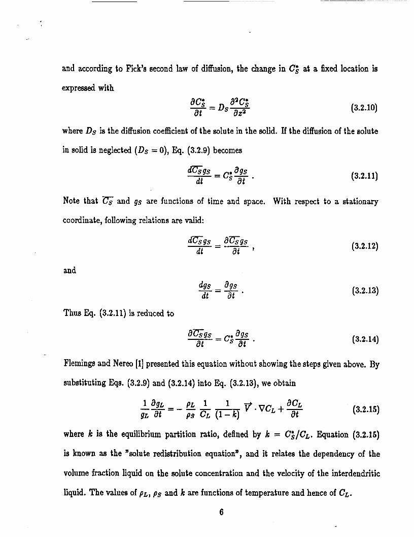
and according to Fick’s second law of diffusion, the change in Cz at a 6x4 location is
expressed with
(3.2.10)
where Ds is the diffusion coefficient of the solute in the solid. If the diffusion of the solute
in solid is neglected (Ds = 0), Eq. (3.2.9) becomes
(3.2.1 1)
Note that and gs are functions of time and space. With respect to a stationary
coordinate, following relations are valid:
G g s a G g s -= dt at ’
and
dgs ags dt at - -=-
Thus Eq. (3.2.11) is reduced to
(3.2.12)
(3.2.13)
(3.2.14)
Flemings and Nereo [l] presented this equation without showing the steps given above. By
substituting Eqs. (3.2.9) and (3.2.14) into Eq. (3.2.13), we obtain
(3.2.15)
where k is the equilibrium partition ratio, defined by k = C;/C,. Equation (3.2.16)
is known as the ”solute redistribution equation”, and it relates the dependency of the
volume fraction liquid on the solute concentration and the velocity of the interdendritic
liquid. The values of pa, ps and k are functions of temperature and hence of CL.
6

3.3 Preseure Equation.
The flow of the interdendritic liquid is expressed with D'Arcy's Law; hence
v = --(VP K - P L T ) P a (3.3.1)
where p is the viscosity of the liquid and K is the permeability of the dendritic network. If
the pressure is considered with reference to atmospheric pressure and the density of liquid
at the liquidus isotherm, we define f' with
then Eq. (3.3.1) can be rewritten
1 J = -- [." - ( p t - p L o ) 7 K PSL
(3.3.2)
(3.3.3)
The two velocity components, Vr and V', in cylindrical coordinate system are given by:
and
1 P9L IC, [" - (PL - PS0)9z Vx = --
(3.3.4)
(3.3.5)
where Kr and Kz are the permeabilities in the r- and 1;-directions, respectively, and gr and
gz are eero and -9, respectively, for vertical solidification.
In cylindrical coordinates the left hand side of Eq. (3.1.6) is
(3.3.6)
7

and substitution of Eqs. (3.3.4) and (3.3.5) into Eq. (3.3.6) leads to the pressure equation,
which is
where
(3.3.7)
It should be pointed out that Kr and Kz each vary within the solid/liquid mne according
to the volume fraction of liquid and the dendrite arm spacings of the dendritic network
141.
3.4 Steady-state Solidification.
Consider a stationary coordinate (r',z') and a moving coordinate system (r,z) with
the velocity (wr, wz). Then a full derivative of a function f with respect to t is given by
(3.4.1)
For steady-state, the function value on a moving frame does not change with time. Thus
we have
(3.4.2)
8

For our application the origin moves such that tur = 0 and UI, = uz, where uz b the
solidification velocity in the s-direction, then Qs. (3.2.15) and (3.3.7) are reduced to the
following expressions:
and
(3.4.3)
Equations (3.4.2) and (3.4.3) are the pressure equation and solute redistribution equation,
respectively, for steady-state solidification.
At r = 0, we evaluate (a,./r) (aP/ar) with L’Hospital’s rule; therefore
(3.4.4)
3.6 Boundary Conditione.
At the liquidus isotherm
If the pressure at r = 0 and at the isotherm is represented with Po, then the pressure
along the liquidus isotherm is
P = Po + P L o g s ( ~ - ZLO) (3.6.1)
where ga is the component of gravity in the s-direction and p~~ is the density of the
interdendritic liquid where CL = Co. In terms of the modified pressure B, related to by
Eq. (3.3.2), this condition becomes
P = 0.
9
(3.5.2)

At the eutectic isotherm
Interdendritic liquid must flow to compensate for the shrinkage associated with the
solidification of the eutectic liquid. Thus,
V,=-u.( PSE - PLE ) ( - t a n s ) , PLE
and
P S E - PLE
PLE
(3.5.3)
(3.5.4)
where 0 is the angle between the tangent to the eutectic isotherm and the horizontal line.
By combining Eqs. (3.3.5, (3.5.3) and (3.5.4), the boundary condition can be expressed in
t e r n of the pressure gradient at the eutectic isotherm
the c enter f -0)
(3.5.5)
(3.5.6)
Since the solid/liquid zone is axisymmetric, the radial component of velocity is Bern.
v r = 0.
Substitution of this equation into Eq. (3.3.4) gives
aP at - = 0. (3.5.7)
At the outer wall (r=R)
The outer wall blocks the movement of the interdendritic liquid in the r-direction.
Thus
v r = 0
10

so in terms of modified pressure,
aP - = o . at (3.5.8)
The boundary conditions are also shown in Figs 3(a) and 3(b). Temperatures at the
eutectic and liquidus isotherms are TE and To, respectively, and the axial symmetry gives
sero heat flux in the radial direction at the center, i.e. BT/Br = 0.
3.6 Energy Equation.
Let’s represent the enthalpy densities for the solid and the interdendrititic liquid with
Qu and QI, respectively. The energy consemtion, taking account of heat conduction and
convection, is
( 3.6.1) a ~ ( q u + QI) = V *(nVT) - V(91v)
where n is the thermal conductivity of the mixture of the solid and liquid. The first term
on the r.h.s. of Eq. (3.6.1) is the energy transported due to conduction and the second
due to the convection of the interdendritic liquid. The enthalpy densities are related to
the enthalpy of the primary solid, IT,, and the enthalpy of the interdendritic liquid, El,
through the equations,
Qa = PsgsHu (3.6.2)
(3.6.3)
If we define the difference in the enthalpies, L, with
L = H l - H ,
11
(3.6.4)

.
then Eq. (3.6.3) becomes
Substituting Eqs. (3.6.2) and (3.6.5) into Eq. (3.6.1) and expanding t e r n , we obtain
(3.6.6)
where 7 is the average density given by Eq. (3.1.2), and inserting Eqs. (3.1.1) and (3.1.2)
into &. (3.6.6) to eliminate V ( p L g L 7 ) terms, we obtain
(3.6.7)
For steady-state solidification and a moving coordinate system with velocity components
= 0 and wz = uZ, we can write
(3.6.8)
where
Equation (3.6.8) is obtained by replacing the t h e derivative terms in Eq. (3.6.7) with
space derivatives via Eq. (3.4.2) and by using the assumptions of a constant solid density
and no porosity formation. The thermal conductivities in the r- and e-directions, nr and
E,, are approximated with the following formulas:
(3.6.9)
12
K Z (1 - g L ) 4 + QLXL (3.6.10)
where the thermal conductivities of the solid and the interdendritic liquid, I C ~ and KL, are
obtained from the thermal data for the pure solids and liquids of the components of the
binary alloy:
CalK81 + c82K82 (3.6.11) &I fil 100
and
(3.6.12) C L ~ K L I + CLaKLa 1co K L fi4
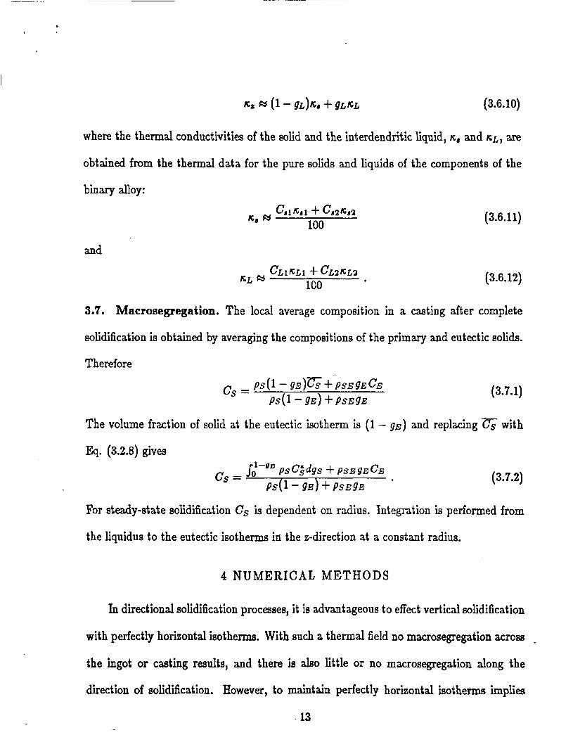
3.7b kfacrosegregation. The locd average composition kt a casting after complete
solidification is obtained by averaging the compositions of the primary and eutectic solids.
Therefore
(3.7.1)
The volume fraction of solid at the eutectic isotherm is (1 - g ~ ) and replacing with
Eq. (3.2.8) gives
(3.7.2)
For steady-state solidification CS is dependent on radius. Integration is performed from
the liquidus to the eutectic isotherms in the 4;-direction at a constant radius.
4 NUMERICAL METHODS
In directional solidification processes, it is advantageous to effect vertical solidification
with perfectly horizontal isotherms. With such a thermal field no macrosegregation acros
the ingot or casting results, and there is also little or no macrosegregation along the
direction of solidification. However, to maintain perfectly horizontal isotherms implies
13

no temperature gradients across the ingot or casting; this, of course, is impossible but is
approximated in practice.
The consequence of slightly curved isotherms is that there can be macrosegregation
across the casting or ingot depending upon solidification rate, the alloy, and the extent
of the concavity or convexity of the isotherms. At high solidification rates, e.g. ud >
5 x lo-’ cm - s-l, a small curvature of the isotherms is expected to be insignificant, but
at low solidification rates, e.g. IO-’ 5 uz 5 IO-‘ cm - rl, even slight curvatures can
profoundly affect the flow of the interdendritic liquid and, thereby, cause macrosegregation.
In the following we discuss first the numerical simulation of a rectangular mesh, which
is appraximate for directional solidification (DS) with horisontal isotherms, and then we
discuss a non-rectangular mesh for adaptation to DS slightly curved isotherms.
The generation of a rectangular mesh is straightforward; however there are some
difficulties in formulating finite difference approximations for boundary points. Fig. 4(a)
shows a rectangular mesh with uniform spacings in the r- and e-directions as employed by
Kou [5]. At the cuwed boundaries there are special cases which require carefully written
finite difference approximations of the derivatives. Usually finite difference equations of
the second order accuracy are mostly considered, and the truncation errors involved in
the approximations are proportional to the square of the grid spacings. In order to retain
accuracy, all points including the boundary points must be expressed with the formulas
of at least the same order of the accuracy of the interior points. For irregular boundary
points, complicated expressions are required and various formulas must be considered for
different cases. As an example, the first derivative of the function normal to the boundary
14

for point A shown in Fig. 4(a) can be expressed with values at its five nearest points and
the point itself to get the second order accuracy of the derivative. The expression must
be dependent on the distances from boundary points to a internal point closest to point
A in the r- and z-directions. It can be seen that point B must be considered in terms of
the six points shown as circles in Fig. 4(a). This kind of treatment necessitates complex
book-keeping.
To overcome the problems of the mesh of Fig. 4(a), Ridder et al.[6] employed a grid
design shown in Fig. 4b) . Vertical lines of equal spacings in the r-direction are drawn
and the horizontal lines are drawn beginning at the intersections of curved boundaries
and the vertical lines, resulting in nonuniform grid spacinjp in the e-direction. Additional
horizontal lines which do not cross the curved boundaries are also inserted if necessary.
This configuration gives computational efficiency and eliminates the burden of complex
book-keeping for the mesh points at the curved boundaries; however, it must be noted
that spacings in the s-directions are dependent on the selection of vertical grid lines, and
the grid spacings of consecutive mesh points may differ by as much as several order of
magnitudes depending on the geometry of the computation domain. This can adversely
affect the accuracy of the solution as well as the convergence properties of the difference
method.
4.1 Nonorthogonal Meah.
A nonorthogonal mesh is shown in Fig. 5. Suppose that we want m intervals in the r-
direction and n intervals in the %-direction; we can start with (n- 1) equally-spaced points
at the center line, i.e., r=O. Arbitrary smooth cuvea are drawn toward the outer wall of the
15
.
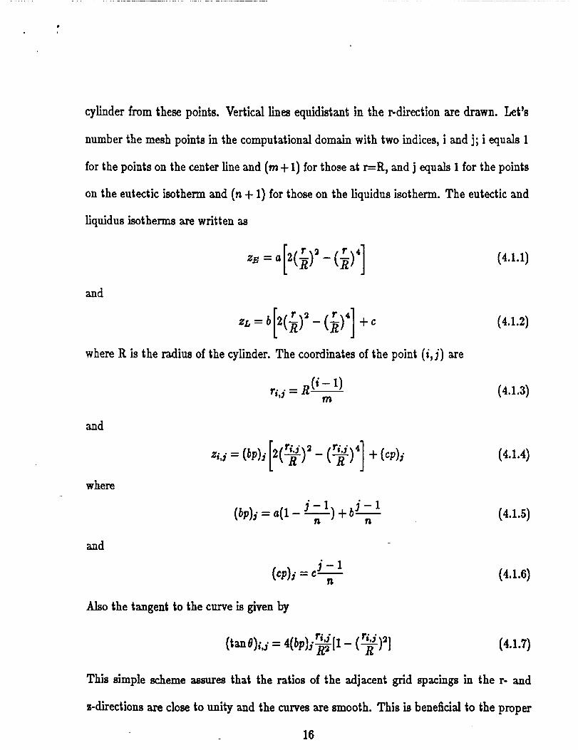
cylinder from these points. Vertical lines equidistant in the rdirection are drawn. Let%
number the mesh points in the computational domain with two indices, i and j; i equals 1
for the points on the center line and (m + 1) for those at r=R, and j equals 1 for the points
on the eutectic isothem and (n + 1) for those on the liquidus isotherm. The eutectic and
liquidus isotherms are written as
and
where R is the radius of the cylinder. The coordinates of the point ( i , j ) are
and
where
and
(i- 1) ri,j = R- m
j-1 j-1 (bp)j = a(1- -) + b- n n
Also the tangent to the curve is given by
(4.1.1)
(4.1.2)
( 4.1.3)
(4.1.4)
(4.1.5)
(4.1.6)
(4.1.7)
This simple scheme assures that the ratios of the adjacent grid spacings in the r- and
s-directions are close to unity and the curves are smooth. This is beneficial to the proper
~ 16

estimation of spatial derivatives, however, it is necessary to consider finite differece a p
proximations that are different than coventional expressions, because the generated mesh
is nonorthogonal. A detailed description of this approximation is given later.
4.2 Generalized Pmite Difference Method.
Conventional finite difference methods divide a computatation domain into rectangu-
lar meshes by positioning mesh points along a curve parallel to either of the orthogonal
axes, and approximate spatial derivatives with several function values along the curve.
Consider the rectangular meshea of the uniform spacings in the r- and e-directions as
shown in Fig. 6(a). Central difference approximations of the first and second derivatives
of a function f at a mesh point (i,j) are represented with the following relations:
and
The derivatives are given in terms of the grid spacings and the function values at neighbor-
ing eight points and the point itself. In matrix notation these equations may be rewritten,
(4.2.1)

where
t o
0
(4.2.2)
0 0 0 0 0 0
0 0 0 0 0 0 0
0.s 0
0 0
and
(4.2.4)
where column vectors (GD) and ( f ~ ) represent the global derivatives and nodal function
values, respectively, and the (TR) a 5 x 9 transformation matrix which makes it possible
to compute (GD) based on nodal function values. Examination of Eq. (4.2.1) shows that
the shape of the matrix (TR) is dependent on Ar and Az. Suppose that the grid lines are
not parallel to the axes of the coordinates. Then, all the zeros in 3. (4.2.1) are expected
to changed to nonzeros. This indicates that (GD) is dependent on the location of the
neighboring points. Instead of taking the center node as a reference, any of the other eight
neghboring nodes can be selected as the reference and employ forward and/or backward
differencing techniques in either of the directions.
The dependency of the (TR) on the coordinates of the neighboring points and the
selection of the reference node has been analysed by Kwok [7]. Each effect of the two factors
1Q

on the matrix (2'8) was obtained by considering a global coordinate and corresponding
local coordinate and the transformation between the coordinate systems. A function f(r,z)
defined in a region of a global r-z plane can be related to the simple local coordinates in the
a-fl plane as shown in Fig. 7. The nine points in the local coordinates are numbered in an
arbitrary order. The coordinate (ai,pi) in the local plane corresponds to the coordinate
( t i , & ) in the global plane. Within the local curvilinear mesh, the function value for an
arbitrary point can be approximated with the following second-order polynomial:
From the equations for the nine nodal points, the coefficients in &. (4.2.5) are known
and then the first and second derivatives with respect to a and fl are given in berms of the
coefficients and the function valuea, ( f ~ ) . If the function in a global plane is appraximated
with a second-order truncated Taylor series expansion, the derivatives in the plane are
expressed in terms of the global coordinates of the nine points and the function values at
these points, ( f ~ ) . The matrix (TR) was obtained by combining the derivatives in the
local and global planes. The relationship between (GD) and ( f ~ ) derived by Kwok [7] is,
(GD) = ((W (m-l (DCI (fd (4.2.6)
where
(4.2.7)
(4.2.8)
19

for the central, forward as well as backward differencing schemes for various cases are
obtained simply by varying m. Other parameters are dependent on m.
Node m
1
2
1 Point
Boundary 1 :
L o c a t i o n
I n t e r n a l A !
3 4
Fig. 8 shows nodes located at the corners and the boundaries of the computation
domain as well as inside the domain. A represents the internal nodes as shown with solid
circles; B, C, D and E represent the nodes along the four sides forming the boundary.
There are also four corner points, F, G, H and I shown with circles. This clasaification is
essential to employ adequate finite difference approximations to the nodes enclosed in the
computational domain.
Dc 6 0 0
1 0 1 : -1 I 0
0 1 -1
Tab le I . C o o r d i n a t e s i n t h e 4-6 p l a n e c o r r e s p o n d i n g t o s e l e c t e d r e f e r e n c e node.
f H t a -1 I I I
-1 1 1
-1
Adequate difference &ernes are obtained by varying only m. For 3n interior point,
a central difference formula is employed; but, for the nodes located along the boundaries
PRECEDING PAGE BLAEK NOT FlLMED 21

and at the cornera, a forward or backward differencing technique is used to retain the
second-order accuracy of the derivative approximations. The proper selection of m for
different casea and corresponding a and @ values dependent on m are listed in Table I.
4.3 Iterative computation.
Physical properties such a8 viscosity, permeability, the density of the solid, and the
density of interdendritic liquid are temperature dependent. The composition of the inter-
dendritic liquid is also related to temperature by the liquidus of the phase diagram. With
temperature and volume fraction liquid in the computational domain specified, the coef-
ficients and the r.h.s. of the pressure equation (Eq. (3.4.2)) can be estimated. Then the
pressures in the domain are obtained, and the velocities, which depend upon the pressure
distribution, are computed using D’Arcy’s Law. The volume fraction of liquid is updated
to satisfy the local solute redistribution equation, and then the temperature is reestimated.
The iteration steps are performed as follows:
1. Start with a linear temperature profile in the e-direction and zero velocity. Solve for
9L*
2. Solve the pressure equation.
3. Check whether the pressure is sufficiently accurate. If the solution is accurate enough,
jump to step 7.
4. Employ D’Arcy’s Law to calculate velocity.
5. Recalculate gL using the local solute redistribution equation.
6. Solve energy equation for temperature and then go back to step 2.
7. Terminate the loop.
22

A detailed description of these steps is given in later subsections.
4.4 Evaluation of CoeBcients m Preeme Equation.
The values of or,, a=, Br and PI defined by Eq. (3.3.8) vary by several orders of
magnitude in the computation domain. The derivatives of these functions are expressed
in terms of their logarithms:
and
(4.4.1)
(4.4.2)
(4.4.3)
(4.4.4)
Finite difference approximations were applied to the logarithms of the respective functions.
4.5 Solution of Presaure Equation.
The first and second derivatives in Eq. (3.4.3) are given by its function values at
the nine nodes according to Eq. (4.2.10). The transformation matrix in Eq. (4.2.10) is
generated for a node and then the derivatives, Bar/ar, aa,/Bz and apz/az, are evaluated
through their logarithms as explained in the previous section. The derivatives apt /az
and agL/Bz are also evaluated. Mow the transformation matrix is utilieed to form a finite
difference equation corresponding the original equation (3.4.3) for the node. The equation
for node ( i , j ) can be written in the form:
9 (4.5.1)
23
where
A(i, j ) = f)i+a,i+l (4.5.2)
and f ( i , j ) is the computed value of the right hand side of equation (3.4.3). The values of
a and p correspond bo the m as shown in 'hble 1. To simplify expressions, let's drop the
indices i and j in l3q. (4.5.1) and rewrite
9 p,s = f (4.5.3) i=1
The internal nodes are handled with Eq. (4.5.3); however, additional considerations
must be given to the nodes located at boundaries. The conditions to be satisfied in
developing a finite difference equation are a) the maintenance of second-order accuracy in
the approximation of the pressure equation Eq. (3.4.3); b) the incorporation of the supplied
boundary condition; and c) the assurance of the stability assembled matrix equation.
The derivative boundary conditions given at the eutectic isotherm, the center, and at
the wall of the cylinder are of concern. The finite difference expressions for the derivatives
ap/ar and aP/az can be written
aP ar =1
and
(4.5.4)
(4.5.5)
respectively, similar to Eq. (4.5.3). These equations also apply to the node (ij). In order
to incorporate the boundary condition at r = 0, we solve &. (4.4.4) for 4,
(4.5.6)
24

and when eliminate f'2 by inserting this equation into &. (4.5.3). Thus,
(4.5.7)
The derivative boundary conditions ar r = R and at the eutectic isotherm, as shown
in Fig. 3(b), are incorporated to the finite difference Q. (4.6.3) by following the same
procedure. When several conditions are to be incorporated, e.g. for the corner points in a
computational domain, the above procedure is repeated to generate a desired equation.
Finite difference approximations for all nodea are arranged to form a matrix equation.
If the appoximations are written in rowfirst order, the equation is
where
(4.5.8)
(4.5.9)
and
For a computational domain diicretized with five intends in the r-direction and five inter-
vals in the 8-direction, the shape of matrix ( A ) would be represented as shown in Fig. 9.
It was not possible to determine the stability of the matrix equation (4.5.8); however,
our test runs showed that (A) satisfies diagonal dominance, a sufficient condition for the
stability of a matrix equation.
25

The Gauss-Seidel method is used to solve the matrix equation. For the five-point
difference formula typically used for a rectangular computational domain, the function
values at node (ij) is updated at each iteration using the values at (i - l,j), (i + l,j),
(i, j - 1) and (i,j + 1). In addition the generalized finite difference method uses function
values at four corner nodes; their contributions are considered to be relatively insignificant.
4.0 Computation of velocitiee.
After solving the pressure equation, the components of velocity, Vr and V,, are com-
puted from Eqs. (3.3.4) and (3.3.5), respectively. However, from a numerical point-of-view,
there is a difficulty in calculating an accurate value of aP/az. Fig. 10 shows a typical plot
of -aP/az and - ( p ~ - p ~ ~ ) gr in the e-direction. The difference of the two values is quite
small compared with their values. If the value of -aP/az is slightly overestimated, e.g.
five percent larger, the dotted line may lie above the solid line, leading to a velocity of
opposite sign, and multiplication with a large coefficient, Kz/(pgL) in E!q. (3.3.5), greatly
magnifies the error. In fact this happened when the derivative was estimated from the
usual second order finite difference formulae. Even the sign of the velocities were reversely
occasionally. This was tested against an analytical solution available for unidirectional
solidification.
To overcome this problem interpolation formulas were developed. A schematic plot of
!’ along the z-direction, shown in Fig. 10, indicates that special consideration is mandatory
due to a rapid change of P. Data points represented with the coordinates (21, pi), (z2,p2), . . . , (zn, f ” ) may be expressed with a polynomial
n- 1 le = CiZi
r=O (4.6.1)
26

where Co, C1, Ca, . . . , Cn-1 are the coefficients which can be readily obtained. Then the
derivative is given by
(4.6.2)
The value of the derivative was estimated with areasonable accuracy from this equation.
4.7 Quadratic Interpolation.
A curve crossing three points ( x l , f ~ ) , ( x a , f a ) and (23,f3) can be interpolated by a
quadratic equation,
f = axa + bx+ c (4.7.1)
with the coefficients a, b and c given by
(4.7.2)
and
where
(4.7.4)
When the relationship between x and f is given with a table of discrete points, it is neces-
sary to employ an interpolation to obtain values of the function at a specified coordinate.
Hence, this interpolation is used to improve the estimation of a function.
4.8 Eetimation of Volume Fraction Liquid.
27

Eq. (3.4.4) may be written
= 9 gL
a2 (4.8.1)
where
By integrating Ea. (4.8.1) setting the lower bound of the integration to z = ZL, g L = 1,
we obtain
(4.8.3)
Fig. 11 shows a typical plot of the variation of the integrand along the z-direction. The
solid dots correspond to the mesh points located along the line of a constant radius. The
quadratic interpolation discussed in previous subsection had 60 be developed and employed.
The solid dots are connected through a amooth cuwe following the interpolation using three
nearest neighboring points, and then integration was performed. The area shown in Fig. 11
is used to evaluate the integral of Eq. (4.8.3) and to obtain gL.
4.9 Temperature Calculation.
The boundary conditions applied to the solution of the energy equation (3.6.8) are
shown in Fig. 3(b). The eutectic and liquidus isotherms are maintained at TE and To,
respectively. At the center of the ingot the thermal gradient in the radial direction is
zero due to axial symmetry. At the wall of the ingot, a proper boundary condition is not
indicated. For this report, we apply a special treatment to the points along the wall.
The radial component of the interdendritic velocity, V,-, is zero at the boundary. Thua,

the energy equation becomes
(4.9.1)
Because we are primarily interested in subtle radial gradient, we ignore radial conduction
terms and keep only those in the e-direction; thus we approximate the behavior along the
wall with
a v an, aT az= a Z aZ tcg-+-- (4.9.2)
4.10 Macrosegregation Calculation.
Refer to the plot of C$ versus gs in the z-direction shown in Fig. 12. Solid dots
correspond to calculated results at mesh points. As gs goes to zero, the dots are more
sparsely distributed. Estimation of the local average composition after complete solidifica-
tion requires the estimation of the area in Fig. 12 according to Eq. (3.7.2). Again a smooth
curve connecting the dots is drawn according to the quadratic interpolation. A numerical
integration for the area under the curve gives the average concentration of solute in the
primary phase after solidification is complete.
4.11 Termination of iteratione.
It is necessary to predict whether the current solution is sufficiently accurate. Repre-
sent the calculated P for a point (i,j) at the nfh iteration level with p,$). The stopping
29

criterion employed is
(4.1 1.1)
where €2 is the tolerance measured in relative error. The summation is done for all mesh
points. The residual e&+') computed at the (n+ 1)th iteration corresponds to $,$I. This
value is used to update f) estimated at the previous iteration, i.e.
(4.1 1.2)
When &. (4.11.1) is satisfied, the iterations are stopped. After the first iteration, however,
the next is done without checking the condition (4.11.1). A maximum number of iteration
is also specified to prevent from accidental infinite looping of the iterations.
5 EMPLOYING THE CODE
The program was written primarily to investigate the effect of a very small deviation
from horizontal liquidus and eutectic isotherms on the macrosegregation of Pb-Sn alloys
for solidification rates ranging from cm-s-'. It is absolutely important to use
adequate data for the density of solid, the density of interdendritic liquid, permeability,
viscosity, dendrite arm spacing, thermal conductivities of solid and interdendritic liquid,
phase diagram, and enthalpies of the solid and the interdendritic liquid. Data for the
Pb-Sn alloys are presented in the APPENDIX. Other binary alloys can be processed by
replacing thermal property data, and similar geometries of solid/liquid eone, consistent
with two-dimensional (r,z) cylindrical coordinates, can be processed by modifying the
grid generation procedure. The program was written in TURBO PASCAL v3.0 (Borland
30
to

International, CA) to run with a PC-DOS operating system. Graphics routines were
developed using TURBO GRAPBIX Vl.0 (Borland International, CA). This program can
be run with IBM PC, XT, AT computers or compatibles with IBM-compatible graphics
adaptor or a Hercules monochrome graphics card. A dot-matrix printer is necessary to get
hardcopies of plots displayed on screen. For higher speed computations, installation of the
8087 (80287 for AT machines) math coprocessor is recommended.
5.1 Program Options (Menus).
When execution of this program is requested, a menu is displayed on the screen and
instructs the operator to make a selection. This menu is reproduced as Fig. 13. A brief
description of each option is given below.
0: Concise description of the program is displayed on screen. This can be sent to
printer by pressing Shift-PrtSc key.
1: Requests the operator to enter the name of the input and output data filenames.
Currently PB-SN.DAT is the only file which can be accessed. After execution of
this option, the name of the files and the message "NO results yet" are displyed
on the screen [Fig. 14).
2: The data read from the parameter file is displyed on the screen (Fig. 16). The
operator can modify any of these parameters or get a hardcopy of the data. The
definitions of the parameters are given below:
CO : weight percent Sn.
R, u, b, ZLO : geometry of the aolid/liquid none (Fig. 5).
uz : solidification rate, cm - a-1.
31

hzte f : ratio of the adjacent grid spacings in the x-direction. The grid spacings
can be gradually reduced by setting it to a value less than unity.
Recommended value ranges from 0.8 to 1.0.
to1 : tolerance allowed given in terms of relative error.
maxitr : maximum number of iterations.
kmodel : permeability model. Several permeability models will be implemented
in future versions; however, there is currently only one option avail-
able.
mmax: number of subintends in the r-direction for the mesh.
nmax : number of s u b i n t e d in the z-direction for the mesh.
ENERGY : Energy equation may be solved (ENERGY=l) or the temperature
variation along the e-direction is assumed to be linear (ENERGY=O).
DEBUG : Intermediate results are displayed on the screen or printer if this vari-
able is not zero. This feature was used to facilitate program debug-
ging.
DEVICE : Intermediate results can be displayed on the screen (DEVICE=O) or
sent to the printer (DEVICE=l). This feature is also used for program
debugging.
3: Now, we return to Fig. 13. The data updated by selecting option 2 is overwritten
to the parameter file.
4: The operator can switch to other input and output paramete files for the program
run. This option would be useful when the program is extended to process
32

various binary alloys.
5: Program is run and intermediate and final results are stored as disk files.
6: Final results are displayed on the screen. Also hardcopies of these results may
be obtained.
7: Exit to the operating system (DOS).
5.2 Output.
The results obtained with the parameters displayed on Fig. 15 are shown in Fig. 16.
The effects of so1idification process parameters on macrosegregation are under analysis.
Here the intent is to merely acquaint the reader with the mechanics of using the program.
Fig. l6(a) shows the mesh and the velocity vectors of the interdendritic liquid. The
center of the ingot (r=O) is to the left, and the wall (r=R) is to the right. Notice that the
isotherma, Fig. 16(b), are slightly convex so the less dense interdendritic liquid, enriched
in Sn, flows toward the center. Fig. 16(c) gives the temperature along the center-line and
along the surface. For this example, it is almost linear, but at greater solidification ve-
locities the deviation from linearity is more noticeable. The outputs likely to be of most
interest to the users of this program, are shown in Figs. 16(d) and (e) for the concentration
of Sn and volume fraction of eutectic, respectively. Consistent with the flow of the inter-
dendritic liquid, Fig. 16(a), the amount of eutectic and the composition increase from the
wall to the center. Finally, other characteristics of the mushy zone are given by Figs. 16(f)
through 16(h).
33

REFERENCES
1. M. C. Flemings and G. E. Nereo: Trana. TMS-AIME, 1967, vol. 239, pp. 1449-61.
2. A. L. Maples and D. R. Poirier: Metall. h., ,1984, vol. 5B, pp. 163-172.
3. M. K. Hubbert: Petroleum Trans., AIME, 1956, vol. 236, pp. 222-239.
4. D. R. Poirier: Metall. Trans. B, 1987, vol. 18B, pp. 245-255.
5. S. Kou: Ph.D. Thesis, Massachusetts Institute of Technology, 1978.
6. S. D. Ridder, S. Kou and R. Mehrabian: Metall. Trans. B, 1981, vol. 12B, pp.
435-447.
7. S. K. Kwok: Computational Techniques and Applications, CTAC-83, Ed. by J. Noye
& C. Fletcher, Elsevier Science Publishing, North-Holland, 1984, pp. 173-181.
8. D. R. Poirier: submitted for publication.
9. H. J. Fecht and J. H. Perepeeko: Metall. Trans. A, vol. 19A, to be published.
10. H. R. Thresh, A. F. Crawley and D. W. G. White: Trans. Met. SOC. AIME, 1968, vol.
242, pp. 819-822.
11. W. D. Drotning: High Temp. Sci., 1979, vol. 11, pp. 265-276.
12. A. E. Schwaneke, W. L. Falke and V. R. Miller:- J. Chem. Eng. Data, 1978, vol. 23,
pp. 298-301.
13. H. R. Thresh and A. F. Crawley: Metall. Trans. 1970, V O ~ . 1, pp. 1531-35.
14. Metals Handbook, 8th edition, vol. 1, Americal Society for Metals, Metals Park, Ohio,
1961, pp. 1064 and 1144.
15. J. T. Mason, J. D. Verhoeven and R. Trivedi: J. of Crystal Growth, 1982, vol. 59,
pp. 516-524.
34 ~ ~~~~

16. E. A. Brandes (ed.): Smithelh Metals Reference Book, 6th ed., Butterworths, London,
1983, pp. 14-1 to 14-2.
17. D. R. Poirier and P. Nandapurkar: submitted for publication.
35

I I
4
S O L I D I
I" I
I
Fig. 1 Vertical solidification of melt in cy1 i iidri cal mol d. -
3G

( START)
t
Solute Redistribution
Equation 9'
F ig . 2 Formula t ion o f f l o w equat ions.
37

Z=Z,
Vr= 0
Z=ZLo
z
vr= 0
r = R
r = R
Fig . 3 Eoundary c o n d i t i o n s g i ven i n ( a ) o r i g i i i a l and (b) t ransformed coo rd ina te systems.
38

z
Fig. 4 Rectangular nicsiies ( a ) uniform spacings i t i bo th directions ( b ) uniform spacings i t i the r-ai rection,
b u t adjusted nununiform spacings i n the z-cl i recti on.
39

/ $ LIQUIDUS ISOTHERM I
I
Z
EUTECT IC ISOTHERM
F i g . 5 Co1;iput.a tiorial iiiesh.
40

( I + l , j.1)
Fig . G F i n i t e d i f f e r e n c e f o r m u l a t i o n s f o r ( a ) an o r thogona l r e c t a n g u l a r mesh, and ( b ) a nonorthogonal i r r e g u l a r mesh.
41

g = 1
p = 0
p =-1
8
4 I
9
oc =-1
3 7
1
5
2 d -
6
d =1
Fig. 7 C u r v i l i n e a r n i n e - p o i n t mesh i n ( a ) g l o b a l r - z plane, and (b) l o c a l 4-13 p lane a t node i .
42

Z
G
H
I
F ig . 8 Classif icat ion of nieSii p o i n t s i n conipu t a t i on doma i n ;
. : internal o : corner x : side
43

Fig. 9 The shape o f matrix A. . : nonzero el emerits. x : elements reduced to zero by incorporating
derivative boundary conditions.
44

N cn n
0
I
ai v I
a z Q
DIFFERENCE
t
Z
Fig . 10 Comparison of -a?/az and -(tL-f",) gz
45

Fig . 11 E s t i m a t i o n of volume f r a c t i o n T iqu id by i n t e g r a t i o n . S o l i d d o t s co r re spond t o mesh p o i n t s .
46

20
15 c. u a Y
10
5
0
. . - . . _ . _ e . . . . . / i.1- .-.: .... . ' :. . ' ... . . . . . . 1.
- . - .. - . . . . . . . - _ - ... - . . . . . . . . . . . . . . . . . . . . - . . . . . . . . . . . - . . _ . . . . . . . . . :. . . . . . . . . . . . . . . . .
. . . . . * . . * . :
. : * . -: . . . . . . . . . . . . , . . . . . . . . . . . . . . , .- . . . . . . . . . . . . . - 1 .
- . . . . . . . . . . . . . . . . . - . :- * - . . . . . . . . . . . . . . . . . . . . . . . . . . . . . . . . * . - . . . . . . . . . . . . . . . . . . . . . . . . . . . . . . . .
. . . . . . . . . . . . . . . . . . . . . . . . . * . . .. - - . . - . . . . . . . . . . . . . . . . . . . . . . . . . . . . . . . . . . . . . . . . . . . . . . . . .: . . I . . . .
0.00 0.25 0.50 0.75 1.00
F i g . 12 P l o t o f C: versus g, i n the z -d i r ec t ion . S o l i d do ts correspond-to mesh p o i n t s .
47

Liisplay bac1:ground i n f o r m a t i o n Read i n p u t parameters Mcldif y i n p u t parameters SAVE. updated p a r ameters Goto o t h e r parameter f i le R u n program P l o t f i n a l r e s u l t s PU1 t
I'd0 parameter d a t a exists.
II'4FUT FILEtlr?l*lE : OUTF'U'T FILEPIAME :
E n t e r your s e l e c t i o n :
Fig . 13 Henu d i s p l a y e d on screen a t the b e g i n n i n g o f program run.

GI. D i s p l a y b a c k g r o u n d i n f o r m a t i o n 1. Head i n p u t p a r a m e t e r s 2. M o d i f y i n p u t p a r a m e t e r s 3 . S a v e u p d a t e d p a r a m e t e r s 4. G o t o o t h e r p a r a m e t e r f i l e
6. Plot f i n a l resul ts 7. Q u i t
E: L). F a n p r o g r a m
INF'UT FILEbIAME : pb-5.n. dat OUTFUT FILEI\IAME : m139
E n t e r y o u r s e l e c t i o n :
Fig. 14 Menu d i s p l a y e d on screen a f t e r s e l e c t i o n o f menu "l", and i n p u t and o u t p u t filenames.
49

1. 2.
4.
6 . 7. 8. 9 .
10. 11. 12. 13. 14. 15.
- L\ . c 4.
CC3 R
b Z L
UZ h= r c f
ma:: 1 t r I: mod e 1
rri m a: : nma::
ENERGY DEBUG
DEV I CE
a
t G 1
PAF:APlETER FIL-E : p b - s n . d a t
C h a n g e d 2 t i m e s . E n t e r .to s t o p c h a n c ~ i n g , E n t e r 1::. 15 t o p i - i n t sc i -pen .
F i g . 15 D i s p l a y o f t h e d a t a r e a d f r o m p a r a m e t e r f i l e when menu " 2 " i s s e l e c t e d . can change t h e i n p u t p a r a m e t e r s .
O p e r a t o r
50

ORIGiNAL PAGE IS OF POOR QUALtTY
.................. ...... .......... ..... ................. ........... ......................
...................... .......... ............ ........... ...... w.
........... ....................... .......... ...
............................ ..... ...................... ........... ........... ........... ...................... ........... ............ ........... ...................... ........... ...... ........... ..... ...................... ......................... ......... ........... ..... ................. ...................... ......... .............. ...........
z
I I uz = 0.0004 cn/s Unax/Uz= 6.91E-QEl
I TE)(PEP..TURES, C
1 .... : L I P i R R 1 - : SOLVED
Uant Hardcopy:
F i g . 16 Ou tpu t o b t a i n e d from t h e p a r a m e t e r s shown i n F i g . 14.
. 51

ORIGiNAL PAGE IS OF POOR QUALfTY
1.70-
1.60-
1.58. - - -
1.40.
1.384 I 1
I 1 8.48 0.68 8.88 0.20 8.63
Hant hardcopy (Y/N) : . r/F!
Fig. 16 (cont inued . )
52

ORlOlMAL PAGE IS OF POOR QUALITY
I 1 I ) 8.40 0.68 8.80 0. a3 0.20
(2-Z) /( ZL-7x1 Nant hardcopy (YA) : -
h 0.80
.
Fig. 16 (continued.)
53

APPENDIX - DATA FOR PB-SN ALLOY
Al l Deneity of Solid.
P S E (density of eutectic solid) = 8.366 g/cm3
ps (average density of solid) = 11.340 - 0.05898 - 0.001273 T
The density of the solid (lead-rich a phase) is determined by Poirier 181 ua.ag lattice
parameters reported by Fecht and Perepeeko 191.
A.2 Density of Liquid.
PLE (density of eutectic liquid) = 7.928 g/cm3
P L = 10.559 - 0.04251 CL
The density of interdendritic liquid is presented as a function of CL by Poirier [8] based
upon reported [10,11,12].
A.3 Viscosity.
p = 0.026 poise- (g - 3-l - cm-')
Thresh and Crawley [13] measured the viscosities of PbSn melts and extrapolated their
results to the liquidus temperatures. They found that, these viscosites are almost constant;
thus an average value is used here.
A.4 Phase Diagram.
Sufficient, number of points were taken from the liquidus and solidus curves of the
PbSn equilibrium phase diagram [14] (Fig. Al) and fitted to polynomials. CL and k are I
k4

I . I
given by,
CL = 61.656 - 41.496 x - 64.929 X' + 34.872 x3
and
k = 0.301 + 0.200 x - 0.443 2' + 0.73 x3
where
1; (T - TE)/(TM - TE)
TE = 183OC .
TM = 327.5 "C
and
CB = 61.9 wt. pct. Sn.
A.6 Primary Dendrite Arm Spacing.
dl = 584 Gt0.303
where dl is in pm, and GL in O C - crn-l. Mason et al. I151 showed that primary dendrite
arm apacings of dendrites in Pb-Sn alloys of various compositions. At low solidification
rates of our interest, the dependency of dl on the solidification rate is small. Their results
also indicate a weak dependency of dl on alloy composition. The empirical formula is for
Pb-40 Sn alloy and a solidification rate of cm 8-l; however, the actual dendrite arm
spacing is expected to be accurate within 10 % . A.6 Permeability of interdendritic liquid.
K = 3.76 x 10-~ 9 2 d,'

Poirier 14) modelled the flow of the interdendritic liquid with Hagen-Poiseuille law and
estimated the relationship baaed on available data.
A.7 Thermal Conductivity.
The thermal conductivities of pure Pb and of Sn in the liquid and solid states, as
functions of temperature, are taken from Brandes [16] and extrapolated to the temperature
range, 183 OC - 327.5 OC as necessary. (See Fig. A2).
tc8 (Pb) = 0.318 - 1.86 x (T - TE)
n1 (Pb) = 0.130 + 1.64 x (T - TE)
IC# (Sn) = 0.606 - 2.99 x (T - TE)
KI (Sn) = 0.290 + 2.01 x IO-4 (2' - TE)
The units of these conductivities are in waft - cm-l - OC-'.
A.8 Enthalpy.
5 = - 4.788 + 0.13868 T + 0.97811 Cs - 1.0332 x lom3 c' + 1.0449 x T Joule/g
Ht = 63.772 + 0.72996 CL - 7.1156 x
+ 3.7147 x Ci - 4.7423 x Ci Joule/g
Poirier and Nandapurkar 1171 evaluated the enthalpies of the dendritic solid and inter-
dendritic liquid of Pb-Sn alloys and found that they are appreciably dependent on alloy
composition. These dependencies were expressed in polynomials reproduced here.

ORlGlNAL PAGE IS OF POOR QUALITY
Fig. A1 The Pb-Sn e q u i l i b r i u m p h a s e diagram 1143.
57

O. 6
0.4
0.2
0.0
ORIGINAL PAGE IS OF POOR QUALITY
I 1 I I I 1
TE = 183 "C
1 I I 4 I I
I I I I
I I I
I I I I
I I I 1 I I
I I
. _ _
i T,= 327.5 "C I I I
I I I * I I
I 1
0 200 400 600 TEMPERATURE. O C
F i g . A2 Thermal conductivities of Pb and Sn i n thc solid and liquid states [167.
58