computer science iicse.unl.edu/~cbourke/computersciencetwo.pdf · · 2017-07-1025 queue-based bfs...
TRANSCRIPT

Computer Science II
Dr. Chris BourkeDepartment of Computer Science & Engineering
University of Nebraska—LincolnLincoln, NE 68588, USA
http://chrisbourke.unl.edu
2017/06/01 13:58:39Version 0.1.0


This book is a draft covering Computer Science II topics as presented in CSCE 156(Computer Science II) at the University of Nebraska—Lincoln.
This work is licensed under a Creative CommonsAttribution-ShareAlike 4.0 International License
i


Contents
1 Introduction 1
2 Object Oriented Programming 32.1 Introduction . . . . . . . . . . . . . . . . . . . . . . . . . . . . . . . . . . . . 32.2 Objects . . . . . . . . . . . . . . . . . . . . . . . . . . . . . . . . . . . . . . . 32.3 The Big Four . . . . . . . . . . . . . . . . . . . . . . . . . . . . . . . . . . . 3
2.3.1 Abstraction . . . . . . . . . . . . . . . . . . . . . . . . . . . . . . . . . 32.3.2 Encapsulation . . . . . . . . . . . . . . . . . . . . . . . . . . . . . . . . 32.3.3 Inheritance . . . . . . . . . . . . . . . . . . . . . . . . . . . . . . . . . 32.3.4 Polymorphism . . . . . . . . . . . . . . . . . . . . . . . . . . . . . . . . 3
3 Relational Databases 5
4 List-Based Data Structures 74.1 Array-Based Lists . . . . . . . . . . . . . . . . . . . . . . . . . . . . . . . . . 8
4.1.1 Designing a Java Implementation . . . . . . . . . . . . . . . . . . . . . 84.2 Linked Lists . . . . . . . . . . . . . . . . . . . . . . . . . . . . . . . . . . . . 16
4.2.1 Designing a Java Implementation . . . . . . . . . . . . . . . . . . . . . 224.2.2 Variations . . . . . . . . . . . . . . . . . . . . . . . . . . . . . . . . . . 26
4.3 Stacks & Queues . . . . . . . . . . . . . . . . . . . . . . . . . . . . . . . . . 284.3.1 Stacks . . . . . . . . . . . . . . . . . . . . . . . . . . . . . . . . . . . . 294.3.2 Queues . . . . . . . . . . . . . . . . . . . . . . . . . . . . . . . . . . . . 334.3.3 Variations . . . . . . . . . . . . . . . . . . . . . . . . . . . . . . . . . . 37
5 Algorithm Analysis 395.1 Introduction . . . . . . . . . . . . . . . . . . . . . . . . . . . . . . . . . . . . 39
5.1.1 Example: Computing a Sum . . . . . . . . . . . . . . . . . . . . . . . . 455.1.2 Example: Computing a Mode . . . . . . . . . . . . . . . . . . . . . . . 47
5.2 Pseudocode . . . . . . . . . . . . . . . . . . . . . . . . . . . . . . . . . . . . 505.3 Analysis . . . . . . . . . . . . . . . . . . . . . . . . . . . . . . . . . . . . . . 525.4 Asymptotics . . . . . . . . . . . . . . . . . . . . . . . . . . . . . . . . . . . . 57
5.4.1 Big-O Analysis . . . . . . . . . . . . . . . . . . . . . . . . . . . . . . . 575.4.2 Other Notations . . . . . . . . . . . . . . . . . . . . . . . . . . . . . . . 595.4.3 Observations . . . . . . . . . . . . . . . . . . . . . . . . . . . . . . . . 615.4.4 Limit Method . . . . . . . . . . . . . . . . . . . . . . . . . . . . . . . . 64
iii

Contents
5.5 Examples . . . . . . . . . . . . . . . . . . . . . . . . . . . . . . . . . . . . . 665.5.1 Linear Search . . . . . . . . . . . . . . . . . . . . . . . . . . . . . . . . 665.5.2 Set Operation: Symmetric Difference . . . . . . . . . . . . . . . . . . . 685.5.3 Euclid’s GCD Algorithm . . . . . . . . . . . . . . . . . . . . . . . . . . 695.5.4 Selection Sort . . . . . . . . . . . . . . . . . . . . . . . . . . . . . . . . 71
5.6 Other Considerations . . . . . . . . . . . . . . . . . . . . . . . . . . . . . . . 725.6.1 Importance of Input Size . . . . . . . . . . . . . . . . . . . . . . . . . . 725.6.2 Control Structures are Not Elementary Operations . . . . . . . . . . . 755.6.3 Average Case Analysis . . . . . . . . . . . . . . . . . . . . . . . . . . . 765.6.4 Amortized Analysis . . . . . . . . . . . . . . . . . . . . . . . . . . . . . 77
5.7 Analysis of Recursive Algorithms . . . . . . . . . . . . . . . . . . . . . . . . 785.7.1 The Master Theorem . . . . . . . . . . . . . . . . . . . . . . . . . . . . 79
6 Trees 836.1 Introduction . . . . . . . . . . . . . . . . . . . . . . . . . . . . . . . . . . . . 836.2 Definitions & Terminology . . . . . . . . . . . . . . . . . . . . . . . . . . . . 836.3 Implementation . . . . . . . . . . . . . . . . . . . . . . . . . . . . . . . . . . 926.4 Tree Traversal . . . . . . . . . . . . . . . . . . . . . . . . . . . . . . . . . . . 93
6.4.1 Preorder Traversal . . . . . . . . . . . . . . . . . . . . . . . . . . . . . 946.4.2 Inorder Traversal . . . . . . . . . . . . . . . . . . . . . . . . . . . . . . 966.4.3 Postorder Traversal . . . . . . . . . . . . . . . . . . . . . . . . . . . . . 996.4.4 Tree Walk Traversal . . . . . . . . . . . . . . . . . . . . . . . . . . . 1036.4.5 Breadth-First Search Traversal . . . . . . . . . . . . . . . . . . . . . 104
6.5 Binary Search Trees . . . . . . . . . . . . . . . . . . . . . . . . . . . . . . . 1076.5.1 Retrieval . . . . . . . . . . . . . . . . . . . . . . . . . . . . . . . . . . 1086.5.2 Insertion . . . . . . . . . . . . . . . . . . . . . . . . . . . . . . . . . . 1106.5.3 Removal . . . . . . . . . . . . . . . . . . . . . . . . . . . . . . . . . . 1106.5.4 In Practice . . . . . . . . . . . . . . . . . . . . . . . . . . . . . . . . 114
6.6 Heaps . . . . . . . . . . . . . . . . . . . . . . . . . . . . . . . . . . . . . . 1156.6.1 Operations . . . . . . . . . . . . . . . . . . . . . . . . . . . . . . . . 1166.6.2 Implementations . . . . . . . . . . . . . . . . . . . . . . . . . . . . . 1216.6.3 Variations . . . . . . . . . . . . . . . . . . . . . . . . . . . . . . . . . 1256.6.4 Applications . . . . . . . . . . . . . . . . . . . . . . . . . . . . . . . . 126
6.7 Exercises . . . . . . . . . . . . . . . . . . . . . . . . . . . . . . . . . . . . . 129
Glossary 131
Acronyms 133
Index 136
References 137
iv

List of Algorithms
1 Insert-At-Head Linked List Operation . . . . . . . . . . . . . . . . . . . . . . 172 Insert Between Two Nodes Operation . . . . . . . . . . . . . . . . . . . . . . 183 Index-Based Retrieval Operation . . . . . . . . . . . . . . . . . . . . . . . . . 204 Key-Based Delete Operation . . . . . . . . . . . . . . . . . . . . . . . . . . . 22
5 Computing the Mean . . . . . . . . . . . . . . . . . . . . . . . . . . . . . . . 516 Computing the Mode . . . . . . . . . . . . . . . . . . . . . . . . . . . . . . . 527 Trivial Sorting (Bad Pseudocode) . . . . . . . . . . . . . . . . . . . . . . . . . 528 Trivially Finding the Minimal Element . . . . . . . . . . . . . . . . . . . . . . 539 Finding the Minimal Element . . . . . . . . . . . . . . . . . . . . . . . . . . . 5310 Linear Search . . . . . . . . . . . . . . . . . . . . . . . . . . . . . . . . . . . . 6711 Symmetric Difference of Two Sets . . . . . . . . . . . . . . . . . . . . . . . . 6812 Euclid’s GCD Algorithm . . . . . . . . . . . . . . . . . . . . . . . . . . . . . . 6913 Selection Sort . . . . . . . . . . . . . . . . . . . . . . . . . . . . . . . . . . . . 7114 Sieve of Eratosthenes . . . . . . . . . . . . . . . . . . . . . . . . . . . . . . . 7315 Fibonacci(n) . . . . . . . . . . . . . . . . . . . . . . . . . . . . . . . . . . . . 7916 Binary Search – Recursive . . . . . . . . . . . . . . . . . . . . . . . . . . . . . 8117 Merge Sort . . . . . . . . . . . . . . . . . . . . . . . . . . . . . . . . . . . . . 81
18 Stack-based Preorder Tree Traversal . . . . . . . . . . . . . . . . . . . . . . . 9519 preOrderTraversal(u): Recursive Preorder Tree Traversal . . . . . . . . . . . . 9620 Stack-based Inorder Tree Traversal . . . . . . . . . . . . . . . . . . . . . . . . 9721 inOrderTraversal(u): Recursive Inorder Tree Traversal . . . . . . . . . . . . . 9922 Stack-based Postorder Tree Traversal . . . . . . . . . . . . . . . . . . . . . . 10023 postOrderTraversal(u): Recursive Postorder Tree Traversal . . . . . . . . . . 10324 Tree Walk based Tree Traversal . . . . . . . . . . . . . . . . . . . . . . . . . 10525 Queue-based BFS Tree Traversal . . . . . . . . . . . . . . . . . . . . . . . . 10626 Search algorithm for a binary search tree . . . . . . . . . . . . . . . . . . . . 11027 Finding the maximum key value in a node’s left subtree. . . . . . . . . . . . 11328 Heapify . . . . . . . . . . . . . . . . . . . . . . . . . . . . . . . . . . . . . . 11729 Find Next Open Spot - Numerical Technique . . . . . . . . . . . . . . . . . 12530 Heap Sort . . . . . . . . . . . . . . . . . . . . . . . . . . . . . . . . . . . . . 127
v


List of Code Samples
4.1 Parameterized Array-Based List in Java . . . . . . . . . . . . . . . . . . . . 144.2 A linked list node Java implementation. Getter and setter methods have
been omitted for readability. A convenience method to determine if a nodehas a next element is included. This implementation uses null as itsterminating value. . . . . . . . . . . . . . . . . . . . . . . . . . . . . . . . . 24
5.1 Summing a collection of integers . . . . . . . . . . . . . . . . . . . . . . . . 425.2 Summation Algorithm 1 . . . . . . . . . . . . . . . . . . . . . . . . . . . . . 455.3 Summation Algorithm 2 . . . . . . . . . . . . . . . . . . . . . . . . . . . . . 455.4 Summation Algorithm 3 . . . . . . . . . . . . . . . . . . . . . . . . . . . . . 455.5 Mode Finding Algorithm 1 . . . . . . . . . . . . . . . . . . . . . . . . . . . 475.6 Mode Finding Algorithm 2 . . . . . . . . . . . . . . . . . . . . . . . . . . . 485.7 Mode Finding Algorithm 3 . . . . . . . . . . . . . . . . . . . . . . . . . . . 495.8 Naive Exponentiation . . . . . . . . . . . . . . . . . . . . . . . . . . . . . . 745.9 Computing an Average . . . . . . . . . . . . . . . . . . . . . . . . . . . . . 75
vii


List of Figures
4.1 A simple linked list containing 3 nodes. . . . . . . . . . . . . . . . . . . . . 174.2 Insert-at-head Operation in a Linked List. We wish to insert a new
element, 42 at the head of the list. . . . . . . . . . . . . . . . . . . . . . . . 184.3 Inserting Between Two Nodes in a Linked List. Here, we wish to insert a
new element 42 between the given two nodes containing 8 and 6. . . . . . . 194.4 Delete Operation in a Linked List . . . . . . . . . . . . . . . . . . . . . . . 214.5 Key-Based Find and Remove Operation. We wish to remove the first node
we find containing 42. . . . . . . . . . . . . . . . . . . . . . . . . . . . . . . 234.6 A Doubly Linked List Example . . . . . . . . . . . . . . . . . . . . . . . . 264.7 A Circularly Linked List Example . . . . . . . . . . . . . . . . . . . . . . . 274.8 An Unrolled Linked List Example . . . . . . . . . . . . . . . . . . . . . . . 284.9 A stack holding integer elements. Push and pop operations are depicted
as happening at the “top” of the stack. In actuality, a stack stored in acomputer’s memory is not really oriented but this visualization is consistentwith a physical stack growing “upwards.” . . . . . . . . . . . . . . . . . . . 30
4.10 An example of a queue. Elements are enqueued at the end of the queueand dequeued from the front of the queue. . . . . . . . . . . . . . . . . . . 34
4.11 Array-Based Queue . . . . . . . . . . . . . . . . . . . . . . . . . . . . . . . 364.12 Producer Consumer Pattern . . . . . . . . . . . . . . . . . . . . . . . . . . 37
5.1 Quadratic Regression of Index-Based Linked List Performance . . . . . . . 445.2 Plot of two functions. . . . . . . . . . . . . . . . . . . . . . . . . . . . . . . 565.3 Expected number of comparisons for various success probabilities p. . . . . 77
6.1 An undirected graph with labeled vertices. . . . . . . . . . . . . . . . . . . 846.2 Several examples of trees. It doesn’t matter how the tree is depicted or
organized, only that it is acyclic. The final example, 6.2(d) represents adisconnected tree, called a forest. . . . . . . . . . . . . . . . . . . . . . . . 86
6.3 Several possible rooted orientations for the tree from Figure 6.2(a). . . . . 876.4 A Tree Node’s Relations. . . . . . . . . . . . . . . . . . . . . . . . . . . . . 896.5 A Binary Tree . . . . . . . . . . . . . . . . . . . . . . . . . . . . . . . . . . 896.6 A complete tree of depth d = 3 which has 1 + 2 + 4 + 8 = 15 nodes. . . . . 906.7 A summation of nodes at each level of a complete binary tree up to depth d.916.8 A small binary tree. . . . . . . . . . . . . . . . . . . . . . . . . . . . . . . . 946.9 A walkthrough of a preorder traversal on the tree from Figure 6.5. . . . . . 956.10 A walkthrough of a inorder traversal on the tree from Figure 6.5. . . . . . . 98
ix

List of Figures
6.11 A walkthrough of a postorder traversal on the tree from Figure 6.5. . . . 1026.12 A tree walk on the tree from Figure 6.8. . . . . . . . . . . . . . . . . . . 1046.13 The three general cases of when to process a node in a tree walk. . . . . 1046.14 A Breadth First Search Example . . . . . . . . . . . . . . . . . . . . . . 1066.15 A Binary Search Tree . . . . . . . . . . . . . . . . . . . . . . . . . . . . . 1086.16 Various Search Examples on a Binary Search Tree . . . . . . . . . . . . . 1096.17 Binary Search Tree Insertion Operation . . . . . . . . . . . . . . . . . . . 1116.18 Binary Search Tree Deletion Operation Exampless . . . . . . . . . . . . . 1136.19 A degenerate binary search tree. . . . . . . . . . . . . . . . . . . . . . . . 1146.20 A min-heap . . . . . . . . . . . . . . . . . . . . . . . . . . . . . . . . . . 1156.21 A Max-heap . . . . . . . . . . . . . . . . . . . . . . . . . . . . . . . . . . 1166.22 An Invalid Max-heap . . . . . . . . . . . . . . . . . . . . . . . . . . . . . 1176.23 Insertion and Heapification . . . . . . . . . . . . . . . . . . . . . . . . . . 1186.24 Another Invalid Heap . . . . . . . . . . . . . . . . . . . . . . . . . . . . . 1196.25 Removal of the root element (getMax) and Heapification . . . . . . . . . 1206.26 Heap Node’s Index Relations . . . . . . . . . . . . . . . . . . . . . . . . . 1226.27 An array implementation of the heap from Figure 6.21 along with the
generalized parent, left, and right child relations. . . . . . . . . . . . . . . 1226.28 Tree-based Heap Analysis . . . . . . . . . . . . . . . . . . . . . . . . . . 124
x

1 Introduction
To Come.
1


2 Object Oriented Programming
2.1 Introduction
To Come.
2.2 Objects
2.3 The Big Four
2.3.1 Abstraction
2.3.2 Encapsulation
2.3.3 Inheritance
2.3.4 Polymorphism
3


3 Relational Databases
To Come.
5


4 List-Based Data Structures
Most programming languages provide some sort of support for storing collections ofsimilar elements. The most common way is to store elements in an array. That is,elements are stored together in a contiguous chunk of memory and individual elementsare accessed using an index. An index represents an offset with respect to the firstelement which is usually stored at index 0 (referred to as zero-indexing).
There are several disadvantages to using arrays, however. In particular, once allocated,the capacity of an array is fixed. It cannot grow to accommodate new elements andit cannot shrink if we end up removing elements. Moreover, we may not need the fullcapacity of the array at any given point in a program, leading to wasted space. Thoughlibraries may provide convenience functions, in general all of the “bookkeeping” in anarray is up to us. If we remove an element in the middle of the array, our data may nolonger be contiguous. If we add an element in the array, we have to make sure to find anavailable spot. Essentially, all of the organization of the array falls to the user.
A much better solution is to use a dynamic data structure called a List. A List is anAbstract Data Type (ADT) that stores elements in an ordered manner. That is, thereis a notion of a “first” element, a “second” element, etc. This is not necessarily thesame thing as being sorted. A list containing the elements 10, 30, 5 is not sorted, but
it is ordered ( 10 is the first element, 30 is the second, and 5 is the third and finalelement). In contrast to an array, the list automatically organizes the elements in someunderlying structure and provides an interface to the user that provides some set of corefunctionality, including:
• A way to add elements to the list
• A way to retrieve elements from the list
• A way to remove elements from the list
in some manner. We’ll examine the specifics later on, but the key aspect to a list is that,in contrast to an array, it dynamically expands and contracts automatically as the useradds/removes elements.
How a list supports this core functionality may vary among different implementations.For example, the list’s interface may allow you to add an element to the beginningof the list, or to the end of the list, or to add the new element at a particular index;or any combination of these options. The retrieval of elements could be supported byproviding an index-based retrieval method or an iterator pattern that would allow a user
7

4 List-Based Data Structures
to conveniently iterate over every element in the list.
In addition, a list may provide secondary functionality as a convenience to users, makingthe implementation more flexible. For example, it may be useful for a user to tell howmany elements are in the list; whether or not it is empty or full (if it is designed to havea constrained capacity). A list might also provide batch methods to allow a user to adda collection of elements to the list rather than just one at a time.
Most languages will provide a list implementation (or several) as part of their standardlibrary. In general, the best practice is to use the built-in implementations unless thereis a very good reason to “roll your own” and create your own implementation. However,understanding how various implementations of lists work and what properties they provideis very important. Different implementations provide advantages and disadvantages andso using the correct one for your particular application may mean the difference betweenan efficient algorithm and an inefficient or even infeasible one.
4.1 Array-Based Lists
Our first implementation is an obvious extension of basic arrays. We’ll still use a basicarray to store data, but we’ll build a data structure around it to implement a full list.The details of how the list works will be encapsulated inside the list and users will interactwith the list through publicly available methods.
The basic idea is that the list will own an array (via composition) with a a certaincapacity. When users add elements to the list, they will be stored in the array. When thearray becomes full, the list will automatically reallocate a new, larger array (giving thelist a larger capacity), copy over all the elements in the old array and then switch to thisnew array. We can also implement the opposite functionality and shrink the array if wedesire.
4.1.1 Designing a Java Implementation
To illustrate this design, consider the basic the following code sample in Java.
1 public class IntegerArrayList
2
3 private int arr[];
4 private int size;
5
6
This array-based list is designed to store integers in the arr array. The second membervariable, size will be used to track the number of elements stored in arr . Note thatthis is not the same thing as the size of the array (that is, arr.length ). Elements
8

4.1 Array-Based Lists
may or may not be stored in each array position. To distinguish between the size of thearray-based list and the size of the internal array, we’ll refer to them as the size andcapacity
To initialize an empty array list, we’ll create a default constructor and instantiate thearray with an initial capacity of 10 elements with an initial size of 0 .
1 public IntegerArrayList()
2 this.arr = new int[10];
3 this.size = 0;
4
Adding Elements
Now let’s design a method to provide a way to add elements. As a first attempt, let’sallow users to add elements to the end of the list. That is, if the list currently containsthe elements 8, 6, 10 and the user adds the element 42 the list will then contain the
elements 8, 6, 10, 42 .
Since the size variable keeps track of number of elements in the list, we can use it todetermine the index at which the element should be inserted. Moreover, once we insertthe element, we’ll need to be sure to increment the size variable since we are increasingthe number of elements in the list. Before we do any of this, however, we need to checkto ensure that the underlying array has enough room to hold the new element and if itdoesn’t, we need to increase the capacity by creating a new array and copying over theold elements. This is all illustrated in the following code snippet.
1 public void addAtEnd(int x)
2
3 //if the array is at capacity, resize it
4 if(this.size == this.arr.length)
5 //create a new array with a larger capacity
6 int newArr = new int[this.arr.length + 10];
7 //copy over all the old elements
8 for(int i=0; i<this.arr.length; i++)
9 newArr[i] = this.arr[i];
10
11 //use the new array
12 this.arr = newArr;
13
14 this.arr[size] = x;
15 this.size++;
16
The astute Java programmer will note that lines 5–12 can be improved by utilizing
9

4 List-Based Data Structures
methods provided by Java’s Arrays class. Adhering to the Don’t Repeat Yourself
(DRY) principle, a better version would be as follows.
1 public void addAtEnd(int x)
2
3 if(this.size == this.arr.length)
4 this.arr = Arrays.copyOf(this.arr, this.arr.length + 10);
5
6 this.arr[size] = x;
7 this.size++;
8
As another variation, we could allow users to add elements at an arbitrary index. Thatis, if the array contained the elements 8, 6, 10 , we could allow the user to insert the
element 42 at any index 0 through 3. The list would automatically shift elements downto accommodate the new element. For example:
• Adding at index 0 would result in 42, 8, 6, 10
• Adding at index 1 would result in 8, 42, 6, 10
• Adding at index 2 would result in 8, 6, 42, 10
• Adding at index 3 would result in 8, 6, 10, 42
Note that though there is no element (initially) at index 3, we still allow the user to“insert” at that index to allow the user to insert the element at the end. However, anyother index should be considered invalid as it would either be invalid (negative) or itwould mean that the data is no longer contiguous. For example, adding 42 at index5 may result in 8, 6, 10, null, null, 42 . Thus, we do some basic index checkingand throw an exception for invalid indices.
10

4.1 Array-Based Lists
1 public void insertAtIndex(int x, int index)
2
3 if(index < 0 || index > this.size)
4 throw new IndexOutOfBoundsException("invalid index: " + index);
5
6
7 if(this.size == this.arr.length)
8 this.arr = Arrays.copyOf(this.arr, this.arr.length + 10);
9
10
11 //start at the end; shift elements to the right to accommodate x
12 for(int i=this.size-1; i>=index; i--)
13 this.arr[i+1] = this.arr[i];
14
15 this.arr[index] = element;
16 this.size++;
17
At this point we note that these two methods have a lot of code in common. In fact, onecould be implemented in terms of the other. Specifically, insertAtIndex is the moregeneral of the two and so addToEnd should use it:
1 public void addAtEnd(int x)
2
3 this.insertAtIndex(x, this.size);
4
This is a big improvement as it reduces the complexity of our code and thus the complexityof testing, maintenance, etc.
Retrieving Elements
In a similar manner, we can allow users to retrieve elements using an index-based retrievalmethod. We will again take care to do index checking, but otherwise returning theelement is straightforward.
1 public void getElement(int index)
2
3 if(index < 0 || index >= this.size)
4 throw new IndexOutOfBoundsException("invalid index: " + index);
5
6 return this.arr[index];
7
11

4 List-Based Data Structures
Removing Elements
When a user removes an element, we want to take care that all the elements remaincontiguous. If the array contains the elements 8, 6, 10 and the user removes 8 . we
want to ensure that the resulting list is 6, 10 and not null, 6, 10 . Likewise, we’llwant to make sure to decrement the size when we remove an element. We’ll also returnthe value that is being removed. The user is free to ignore it if they don’t want it, butthis makes the list interface a bit more flexible as it means that the user doesn’t have tomake two method calls to retrieve-then-delete the elements. This is a common idiomwith many collection data structures.
1 public int removeAtIndex(int index)
2
3 if(index < 0 || index > this.size)
4 throw new IndexOutOfBoundsException("invalid index: " + index);
5
6
7 //start at index and shift elements to the left
8 for(int i=index; i<size-1; i++)
9 this.arr[i] = this.arr[i+1];
10
11 this.size--;
12
Note that we omitted automatically “shrinking” the underlying array if its unusedcapacity became too big. We leave that and other variations on the core functionality asan exercise.
Secondary Functionality
In addition to the core functionality of a list, you could extend our design to provide moreconvenience methods to make the list implementation even more flexible. For example,you may implement the following methods, the details of which are left as an exercise.
• public boolean isEmpty() – this method would return true if no elements
were stored in the list, false otherwise.
• public int size() – more generally, a user may want to know how many ele-
ments are in the list especially if they wanted to avoid an IndexOutOfBoundsException .
• public void addAtBeginning(int element) – the companion to the addAtEnd(int)
method
• public int replaceElementAt(int element, int index) – a variation on theremove method that replaces rather than remove the element, returning the replaced
12

4.1 Array-Based Lists
element.
• public void addAll(int arr[], int index) – a batch method that allows auser to add entire array to the list with one method call. Similarly, you could allowthe user to add elements stored in another list instance,public void addAll(IntegerArrayList list, int index) . Sometimes thisoperation is referred to as “splicing.”
• public void clear() – another batch method that allows a user to remove allelements at once.
Many other possible variations exist. In addition to the interface, one could vary howthe underlying array expands or shrinks to accommodate additions and deletions. In theexample above, we increased the size by a constant size of 10. Variations may includeexpanding the array by a certain percentage or doubling it in size each time. Eachstrategy has its own advantages and disadvantages.
A Better Implementation
The preceding list design was still very limited in that it only allowed the user to storeintegers. If we wanted to design a list to hold floating point numbers, strings, or auser defined type, we would need to create an implementation for every possible typethat we wanted a list for. Obviously this is not a good approach. Each implementationwould only differ in its name and the type of elements it stored in its array. This is aquintessential example of when to use parameterized polymorphism. Instead of designinga list that holds a particular type of element, we can parameterize it to hold any type ofelement. Thus, only one array-based list implementation is needed.
In the example we designed before for integers, we never actually examined the contentof the array inside the class. We never used the fact that the underlying array heldintegers and the only time we referred to the int type was in the method signatureswhich can all be parameterized to accept and return the same type.
Code Sample 4.1 contains a parameterized version of the array-based list we implementedbefore.
13

4 List-Based Data Structures
1 public class ArrayList<T>
2
3 private T[] arr;
4 private int size;
5
6 public ArrayList()
7 this.arr = (T[]) new Object[10];
8 this.size = 0;
9
10
11 public T getElement(int index)
12
13 if(index < 0 || index >= this.size)
14 throw new IndexOutOfBoundsException("invalid index: " + index);
15
16 return this.arr[index];
17
18
19 public void removeAtIndex(int index)
20
21 if(index < 0 || index >= size)
22 throw new IndexOutOfBoundsException("invalid index: " + index);
23
24
25 for(int i=index; i<size-1; i++)
26 this.arr[i] = this.arr[i+1];
27
28 this.size--;
29
30
31 public void insertAtIndex(T x, int index)
32 if(index < 0 || index > size)
33 throw new IndexOutOfBoundsException("invalid index: " + index);
34
35
36 if(this.size == arr.length)
37 this.arr = Arrays.copyOf(this.arr, this.arr.length + 10);
38
39
40 for(int i=this.size-1; i>=index; i--)
41 this.arr[i+1] = this.arr[i];
42
43 this.arr[index] = element;
44 this.size++;
45
46
47 public void addAtEnd(T x)
48 this.insertAtIndex(x, this.size);
49
50
Code Sample 4.1: Parameterized Array-Based List in Java
14

4.1 Array-Based Lists
A few things to note about this parameterized implementation. First, with the originalimplementation since we were storing primitive int elements, null was not an issue.Now that we are using parameterized types, a user would be able to store null elementsin our list. We could make the design decision to allow this or disallow it (by adding nullpointer checks on the add/insert methods).
Another issue, particular to Java, is the instantiation of the array on line 7. We cannotinvoke the new keyword on an array with an indeterminate type. This is becausedifferent types require a different number of bytes (integers take 4 bytes, double s take8 bytes). The number of bytes may even vary between Java Virtual Machine (JVM)s(32-bit vs. 64-bit). Without knowing how many bytes each element takes, it would beimpossible for the JVM to allocate the right amount of memory. Thus, we are forced touse a raw type (the Object type) and do an explicit type cast. This is not much of anissue because the parameterizations guarantee that the user would only ever be able toadd elements of type T .
Another useful feature that we could add would be an iterator pattern. An iterator allowsyou to iterate over each element in a collection and process them. With a traditionalarray, a simple for loop can be used to iterate over elements. An iterator pattern relievesthe user of the need to write such boilerplate code and instead use a foreach loop.1
In Java, an iterator pattern is achieved by implementing the Iterable<T> interface(which is also parameterized). The interface requires the implantation of a public methodthat returns an Iterator<T> which has several methods that need to be implemented.The following is an example that could be included in our ArrayList implementation.
1 public Iterator<T> iterator()
2 return new Iterator<T>()
3 private int currentIndex = 0;
4 @Override
5 public boolean hasNext()
6 return (this.currentIndex < size);
7
8
9 @Override
10 public T next()
11 this.currentIndex++;
12 return arr[currentIndex-1];
13
14
15 ;
16
1Note that this is not necessarily mere syntactic sugar. As we will see later, some collections areunordered and would require the use of such a pattern. Yet still, some list implementations, inparticular linked lists, an index-based get method is actually very inefficient. An iterator patternallows you to encapsulate the most efficient logic for iterating over a particular list implementation.
15

4 List-Based Data Structures
Essentially, the iterator (an anonymous class declaration/definition) has an internal index,currentIndex that is initialized to 0 (the first element). Each time next() is called,the “current” element is returned, but the method also sets itself up for the next iterationby incrementing currentIndex . The main advantage of implementing an iterator isthat you can then use a foreach loop (which Java calls an “enhanced for-loop”). Forexample:
1 ArrayList<Integer> list = new ArrayList<Integer>();
2 list.addAtEnd(8);
3 list.addAtEnd(6);
4 list.addAtEnd(10);
5
6 //prints "8 6 10"
7 for(Integer x : list)
8 System.out.print(x + " ");
9
4.2 Linked Lists
The array-based list implementation offers a lot of advantages and improvements over aprimitive array. However, it comes at some cost. In particular, when we need to expandthe underlying array, we have to create a new array and copy over every last element. Ifthere were 1 million elements in the underlying array and we wanted to add one more,we would essentially be performing 1 million copy operations. In general, if there are nelements, we would be performing n copy operations (or a copy operation proportionalto n). That is, some operations will induce a linear amount of work with respect to howmany elements are already in the list. Even with different strategies for increasing thesize of the underlying array (increasing the size by a percentage or doubling it), we stillhave some built-in overhead cost associated with the basic list operations.
For many applications this cost is well-worth it. A copy operation can be performedquite efficiently and the advantages that a list data structure provide to developmentmay outweigh the efficiency issues (and in any case, the same issues would be presenteven if we used a primitive array). In some applications, however, an alternativeimplementation may be more desirable. In particular, a linked list implementation avoidsthe expansion/shrinking of an underlying array as it uses a series of linked nodes to storeelements rather than a primitive array.
A simple linked list is depicted in Figure 4.1. Each element is stored in a node. Eachnode contains both an element (in this example, an integer) and a reference to the nextnode in the list. In this way, each node is linked together to form a chain. The startof the list is usually referred to as the head of the list. Similarly, the end of the list isusually referred to as the tail (in this case, the node containing 10). A special symbolor value is usually used to denote the end of the list so that that tail node does not
16

4.2 Linked Lists
8 6 10 φ
head
Figure 4.1: A simple linked list containing 3 nodes.
point to another node. In this case, we’ve used the value φ to indicate the end of thelist. In practice, a null value could be used or a special sentinel node can be createdto indicate the end of a list.
To understand how a linked list works, we’ll design several algorithms to support thecore functionality of a list data structure. In order to refer to nodes and their elements,we’ll use the following notation. Suppose that u is a node, then its value will be referredto as u.value and the next node it is linked to will be referred to as u.next.
Adding Elements
With a linked list, there is no underlying array of a fixed size. To add an element, wesimply need to create a new node and link it somewhere in the chain. Since there is nofixed array space to fill up, we no longer have to worry about expanding/shrinking it toaccommodate new elements.
To start, an empty list will be represented by having the head reference refer to thespecial end-of-list symbol. That is, head→ φ. To add a new element to an empty list,we simply create a new node and have the head reference point to it. In fact, we canmore generally support an insert at head operation with the same idea. To insert at thehead of the list, we create a new node containing the inserted value, make it point to the“old head” node of the list and then update the head reference to the new node. Thisoperation is depicted in Algorithm 1.
Input :A linked list L with head, L.head and a new element to insert x at thehead
1 u← a new node
2 u.value← x
3 u.next← L.head
4 L.head← u
Algorithm 1: Insert-At-Head Linked List Operation
Just as with the array-based list, we could also support a more general insert-at-index
17

4 List-Based Data Structures
8 6
head
(a) Initially the linked list has element 8 as itshead.
42 8 6
head
(b) We create a new node containing 42
42 8 6
head
(c) We then make the new node refer to the oldhead node.
42 8 6
head
(d) And finally update the head reference topoint to the new node instead.
Figure 4.2: Insert-at-head Operation in a Linked List. We wish to insert a new element,42 at the head of the list.
method that would allow the user to insert a new node at any position in the list. Thefirst step, of course, would be to find the two nodes between which you wanted to insertthe new node. We will save the details for this procedure as it represents a more generalretrieval method. For now, suppose we have two nodes, a, b and we wish to insert a newnode, u between them. To do this, we simply need to make a refer to the new nodeand to make the new node refer to b. However, we must be careful with the order inwhich we do this so as not to lose a’s reference to b. The general procedure is depictedin Algorithm 2.
Input :Two linked nodes, a, b in a linked list and a new value, x to insertbetween them
1 u← a new node
2 u.value← x
3 u.next← a.next
4 a.next← u
Algorithm 2: Insert Between Two Nodes Operation
One special corner case occurs when we want to insert at the end of a list. In thisscenario, b would not exist and so a.next would end up referring to φ. This ends upworking out with the algorithm presented. We never actually made any explicit referenceto b in Algorithm 2. When we assigned u.next to refer to a.next, we took care of boththe possibility that it was an actual node and the possibility that it was φ.
18

4.2 Linked Lists
8 6
42
(a) We create a new node containing 42
8 6
42
(b) We then make the new node point to the secondnode
8 6
42
(c) And reassign the first node’s next reference to thenew node.
8 42 6
(d) Resulting in the new node being inserted betweenthe two given nodes.
Figure 4.3: Inserting Between Two Nodes in a Linked List. Here, we wish to insert anew element 42 between the given two nodes containing 8 and 6.
Another corner case occurs if we wish to insert at the head of the list using this algorithm.In that scenario, a would not refer to an actual node while b would refer to the headelement. In this case, lines 3–4 would be invalid as a.next would be an invalid reference.For this corner case, we would need to either fall back to our first insert-at-head (Algorithm1) operation or we would need to handle it separately.
Retrieving Elements
As previously noted, a linked list avoids the cost of expanding/shrinking of an underlyingarray. However, this does come at a cost. With an array-based list, we had “free” randomaccess to elements. That is, if we wanted the element stored at index i it is a simplematter to compute a memory offset and “jump” to the proper memory location. With alinked list, we do not have the advantages of random access.
Instead, to retrieve an element, we must sequentially search through the list, starting fromthe head, until we find the element that we are trying to retrieve. Again, many variationsexist, but we’ll illustrate the basic functionality by describing the same index-basedretrieval method as before.
The key to this algorithm is to simply keep track of the “current” node. Each iterationwe traverse to the next node in the chain and iterate a counter. When we have traversedi times, we stop as that is the node we are looking for.
In contrast to the “free” index-based retrieval method with an array-based list, the
19

4 List-Based Data Structures
Input :A linked list L with head, L.head and in index i, 0 ≤ i < n where n isthe number of elements in L
Output :The i-th node in L
1 currentNode← L.head
2 currentIndex← 0
3 while currentIndex < i do4 currentNode← currentNode.next
5 currentIndex← (currentIndex+ 1)
6 end
7 output currentNode
Algorithm 3: Index-Based Retrieval Operation
operation of finding the i-th node in a linked list is much more expensive. We have toperform i operations to get the i-th node. In the worst case, when we are trying toretrieve the last (tail) element, we would end up performing n traversal operations. Ifthe linked list held a lot of elements, say 1 million, then this could be quite expensive.In this manner, we see some clear trade-offs in the two implementations.
Removing Elements
Like the insertion operation, the removal of an element begins by retrieving the nodethat contains it. Suppose we have found a node, u and wish to remove it. It actuallysuffices to simply circumvent the node, by making u’s predecessor point to u’s successor.This is illustrated in Figure 4.4.
Since we are changing a reference in u’s predecessor, however, we must make appropriatechanges to the retrieval operation we developed before. In particular, we must keep trackof two nodes: the current node as before but also its predecessor, or more generally, aprevious node. Alternatively, if we were performing an index-based removal operation,we could easily find the predecessor by adjusting our index. If we wanted to delete thei-th node, we could retrieve the (i− 1)-th node and delete the next one in the list.
Again, we may need to deal with corner cases such as if we are deleting the head of thelist or the tail of the list. As with the insertion, the case in which we delete the tail isessentially the same as the general case. If the successor of a tail node is φ, thus whenwe make u’s predecessor refer to u’s successor, we are simply making it refer to φ.
The more complicated part is when we delete the head of the list. By definition, there isno predecessor to the head, so handling it as the general case will result in an invalidreference. Instead, if we wanted to delete the head, we must actually change the list’shead itself. This is easy enough, we simply need to make head refer to head− > next.
20

4.2 Linked Lists
8 6 10
Node to delete
(a) We wish to delete the node containing 6.
8 6 10
(b) We make its predecessor node point to its successor.
8 10
(c) Though the node containing 6 still refers to thenext node, from the perspective of the list, it hasbeen removed.
Figure 4.4: Delete Operation in a Linked List
21

4 List-Based Data Structures
An example of a removal operation is presented in Algorithm 4. In contrast to previousexamples, this operation is a key-based removal operation variation. That is, we searchfor the first instance of a node whose value matches a given key element and delete it.As another corner case for this variation, we also must deal with the situation in whichno node matches the given key. In this case, we’ve decided to leave it as a no-operation(“noop”). This is achieved in lines 10–12 which will not delete the last node if the keydoes not match.
Input :A linked list L with head, L.head and a key element k
Output :L but with the first node u such that u.value = k removed if one exists
1 if L.head.value = k then2 L.head.← L.head.next
3 else4 previousNode← φ
5 currentNode← L.head
6 while currentNode.value 6= k and currentNode.next 6= φ do7 previousNode← currentNode
8 currentNode← currentNode.next
9 end
10 if currentNode.value = k then11 previousNode.next← currentNode.next
12 end
13 end
14 output L
Algorithm 4: Key-Based Delete Operation
4.2.1 Designing a Java Implementation
We now adapt these operations and algorithms to design a Java implementation ofa linked list. Note that the standard collections library has both an array-based list( java.util.ArrayList<E> ) as well as a linked list implementation ( java.util.LinkedList<E> )that should be used in general.
First, we need a node class in order to hold elements as well as a reference to anothernode. Code Sample 4.2 gives a basic implementation with several convenience methods.The class is parameterized so that nodes can hold any type.
Given this Node class, we can now define the basic state of our linked list implementation:
22

4.2 Linked Lists
8 6 10 42 7
currentprevious
φ
(a) Initialization of the previous and current references.
8 6 10 42 7
currentprevious
(b) After the first iteration of the while loop, the references have been updated.
8 6 10 42 7
currentprevious
(c) After the second iteration of the while loop.
8 6 10 42 7
currentprevious
(d) After the third iteration, the current node matches our key value, 42 and the loop terminates.
8 6 10 42 7
currentprevious
(e) Since the current node matches the key, we remove it by circumventing it.
8 6 10 7
(f) Resulting in the node’s removal.
Figure 4.5: Key-Based Find and Remove Operation. We wish to remove the first nodewe find containing 42.
23

4 List-Based Data Structures
1 public class Node<T>
2
3 private final T item;
4 private Node<T> next;
5
6 public Node(T item)
7 this.item = item;
8 next = null;
9
10
11 //getters and setters omitted
12
13 public boolean hasNext()
14 return (this.next == null);
15
16
17
Code Sample 4.2: A linked list node Java implementation. Getter and setter methodshave been omitted for readability. A convenience method to determineif a node has a next element is included. This implementation usesnull as its terminating value.
1 public class LinkedList<T>
2
3 private Node<T> head;
4 private int size;
5
6 public LinkedList()
7 this.head = null;
8 this.size = 0;
9
10
11 ...
12
13
We keep track of the size of the list and increment/decrement it on each add/deleteoperation so that we do not have to recompute it. To keep things simple, we willimplement a two general purpose node retrieval methods, one index-based and one keybased. These can be used as basic steps in other, more specific operations such asinsertion, retrieval, and deletion methods. Note that both of these methods are private
as they are intended for “internal” use by the class and not for external use. If we hadmade these methods public we would be exposing the internal structure of our linked
24

4.2 Linked Lists
list to outside code. Such a design would be a typical example of a leaky abstraction andis, in general, considered bad practice and bad design.
1 private Node<T> getNodeAtIndex(int index)
2
3 if(index < 0 || index >= this.size)
4 throw new IndexOutOfBoundsException("invalid index: " + index);
5
6 Node<T> curr = this.head;
7 for(int i=0; i<index; i++)
8 curr = curr.getNext();
9
10 return curr;
11
12
13
14 private void getNodeWithValue(T key)
15
16 Node<T> curr = head;
17 while(curr != null && !curr.getItem().equals(key))
18 curr = curr.getNext();
19
20 return curr;
21
As previously mentioned, these two general purpose methods can be used or adaptedto implement other, more specific operations. For example, index-based retrieval andremoval methods become very easy to implement using these methods as subroutines.
1 public T getElement(int index)
2 return getNodeAtIndex(index).getItem();
3
4
5 public T removeAtIndex(int index)
6
7 if(index < 0 || index >= this.size)
8 throw new IndexOutOfBoundsException("invalid index: " + index);
9
10 Node<T> previous = getNodeAtIndex(index-1);
11 Node<T> current = previous.getNext();
12 T removedItem = current.getItem();
13 previous.setNext(current.getNext());
14 return removedItem;
15
Adapting these methods and using them to implement other operations is left as an
25

4 List-Based Data Structures
φ 8 6 10 φ
head tail
Figure 4.6: A Doubly Linked List Example
exercise.
4.2.2 Variations
In addition to the basic linked list data structure design, there are several variationsthat have different properties that may be useful in various applications. For example,one simple variation would be to not only keep track of the head element, but also atail element. This would allow you to efficiently add elements to either end of the listwithout having to traverse the entire list. Other variations are more substantial and wewill not look at several of them.
Doubly Linked Lists
As presented, a linked list is “one-way.” That is, we can only traverse forward in the listfrom the head toward the tail. This is because our tree nodes only kept track of a nextelement, referring to the node’s predecessory. As an alternative, our list nodes couldkeep track of both the next element as well as a previous element so that it has access toboth a node’s predecessor as well as its successor. This allows us to traverse the list twoways, forwards and backwards. This variation is referred to as a doubly linked list.
An example of a doubly linked list is depicted in Figure 4.6. In this example, we’ve alsoestablished a reference to the tail element to enable us to start at the end of the list andtraverse backwards.
A doubly linked list may provide several advantages over a singly linked list. For example,when we designed our key-based delete operation we had to be sure to keep track of aprevious element in order to manipulate its reference to the next node. In a doubly linkedlist, however, since we can always traverse to the previous node this is not necessary.
A doubly linked list has the potential to simplify a lot of algorithms, however it alsomeans that we have to take greater care when we manipulate the next and previousreferences. For example, to insert a new node, we would have to modify up to fourreferences rather than just two. Greater care must also be taken with respect to cornercases.
26

4.2 Linked Lists
8 6 10
head
Figure 4.7: A Circularly Linked List Example
Circularly Linked Lists
Another variation is a circularly linked list. Instead of a ending the list using a sentinelvalue, φ, the “last” node points back to the first node, closing the list into a large loop.An example is given in Figure 4.7. With such a structure, it is less clear that there is ahead or tail to the list. Certain operations such as index-based operations may no longermake sense with such an implementation. However, we could still designate an arbitrarynode in the list as the “head” as in the figure.
Alternatively, we could instead simply have a reference to a current node. At any pointduring the data structure’s life cycle the current node may reference any node in the list.The core operations may iterate through the list and end up at a different node eachtime. Care would have to be taken to ensure that operations such as searching do notresult in an infinite loop, however. An unsuccessful key-based search operation wouldneed to know when to terminate (when it has gone through the entire circle once andreturned to where it started). It is easy enough to keep track of the size of the list andto ensure that no circular operations exceed this size.
Circularly linked lists are useful for applications where elements must be processed overand over each in turn. For example, an operating system may give time slices to runningapplications. Instead of a well-defined beginning and end, a continuous poll loop is run.When the “last” application has exhausted its time slot, the operating system returns tothe “first” in a continuous loop.
Unrolled Linked Lists
As presented, each node in a linked list holds a single element. However, we could designa node to hold any number of elements, in particular an array of m elements. Nodeswould still be linked together, but each node would be a mini array-based list as well.An example is presented in Figure 4.8.
This hybrid approach is intended to achieve better performance with respect to memory.The size of each node may be designed to be limited to fit in a particular cache line, theamount of data typically transferred from main memory to a processor’s cache. The goalis to improve cache performance while reducing the overhead of a typical linked list. In a
27

4 List-Based Data Structures
81 16 · · · 10 32
21 42 · · · 89 47
13 17 · · · 21 18 φ
head
m elements
Figure 4.8: An Unrolled Linked List Example
typical linked list, every node has a reference (or two in the case of doubly linked lists)which can double the amount of memory required to store elements. By storing moreelements in each node, the overall number of nodes is reduced and thus the number ofreferences is reduced. At the same time, an unrolled linked list does not require largechunks of contiguous storage like an array-based list but provides some of the advantages(such as random access within a node). Overall, the goal of an unrolled linked list is toreduce the number of cache misses required to retrieve a particular element.
4.3 Stacks & Queues
Collection data structures such as lists are typically unstructured. A list, whether array-based, a linked list, or some other variation simply hold elements in an ordered manner.That is, there is a notion of a first element, second element, etc. However that orderingis not necessarily structured, it is simply the order in which the elements were added tothe collection. In contrast, you can impose a structured ordering by sorting a list (thus,“sorted” is not the same thing as “ordered”). Sorting a list, however, does not give thedata structure itself any more structure. The interface would still allow a user to insertor rearrange the elements so that they are no longer sorted. Sorting a list only change’sthe collection’s state, not its behavior.
We now turn our attention to a different kind of collection data structure whose structureis defined by its behavior rather than its state. In particular, we will look at two datastructures, stack and queues, that represent restricted access data structures. These datastructures still store elements, but the general core functionality of a list (the abilityto add, retrieve, and remove arbitrary elements) will be restricted in a very particularmanner so as to give the data structure behavioral properties. This restriction is builtinto the data structure as part of the object’s interface. That is, users may only interact
28

4.3 Stacks & Queues
with the collection in very specific ways. In this manner, structure is imposed throughthe collection’s behavior.
4.3.1 Stacks
A stack is a data structure that stores elements in a last-in, first-out (or Last-In First-Out(LIFO) manner. That is, the last element to be inserted into a stack is the first elementthat will come out of the stack. A stack data structure can be described as a stack ofdishes. When dealing with such a stack, we can add a dish to it, but only at the top ofthe stack lest we risk causing the entire stack of dish to fall and break. Likewise, whenremoving a dish, we remove the top-most dish rather than pulling a dish from the middleor bottom of the stack for the same reason. Thus, the last dish that we added to thestack will be the first dish that we take off the stack. It may also be helpful to visualizesuch a stack of dishes as in a cafeteria where a spring-loaded cart holds the stack. Whenwe add a dish, the entire stack moves down into the cart and when we remove one, thenext one “pops” up to the top of the stack.
You are probably already familiar with the concept of stacks in the context of a program’scall stack. As a program invokes functions, a new stack frame is created that contains allthe “local” information (parameters, local variables, etc.) and is placed on top of the callstack. When a function is done executing and returns control back to the calling functionthe stack frame is removed from the top of the call stack, restoring the stack frame rightbelow it. In this manner, information can be saved and restored from function call tofunction call efficiently. This idea goes all the way back to the very earliest computersand programming languages (specifically, the Information Processing Language in 1956).
Core Functionality
In order to have achieve the LIFO behavior, access to a stack’s elements are restrictedthrough its interface by only allowing two core operations:
• push adds a new element to the stop of the stack and
• pop removes the element at the top of the stack
The element removed at the top of the stack may also be “returned” in the context of amethod call.
Similar to lists, stacks also have several corner cases that need to be considered. First,when implementing a stack you must consider what will happen when a user performsa pop operation on an empty stack. Obviously there is nothing to remove from thestack, but how might we handle this situation? In general, such an invalid operation isreferred to as a stack underflow. In programming languages that support error handlingvia exceptions, we could choose to throw an exception. If we were to make this designdecisions then we should, in addition, provide a way for the user to check that such an
29

4 List-Based Data Structures
8
6
10
42
3
7
Bottom
Top
push pop
Figure 4.9: A stack holding integer elements. Push and pop operations are depictedas happening at the “top” of the stack. In actuality, a stack stored in acomputer’s memory is not really oriented but this visualization is consistentwith a physical stack growing “upwards.”
30

4.3 Stacks & Queues
operation may result in an exception by providing a way for them to check if the stack isempty or not (see Secondary Functionality below). Alternatively, we could instead returna “flag” value such as null to indicate an empty stack. Though this design decision hasconsequences as well: we would either need to disallow the user from pushing a null
value onto the stack (and decide how again to handle that) or we would need to providea way for the user to distinguish the situation where null was actually popped off thestack or was returned because the stack was empty.
In addition, we could design our stack to be either bounded or unbounded. An unboundedstack means that there would be no practical restrictions on how large the stack couldgrow. A program’s use of our stack would only be limited by the amount of systemmemory available. A user could continue to push as many elements onto the stack asthey like and a problem would only arise when the program or system itself runs out ofmemory.
A bounded stack means that we could design our stack to have a fixed capacity or limitof (say) n elements. If we went with such a design we would again have to deal withthe corner case of a user pushing an element to the stack when it is full referred to asa stack overflow. Solutions similar to the popping from an empty stack could be usedhere as well. We could throw an exception (and give the user the ability to check if thestack is full or not) or we could make such an operation a no-op: we would not push theelement to the stack, leaving it as it was before and then report the no operation to theuser. Typically a boolean value is used, true to indicate that the operation was validand had some side effect on the stack (the element was added) or false to indicate thatthe operation resulted in no side effects.
Secondary Functionality
To make a stack more versatile it is common to include secondary functionality such asthe following.
• A peek method that allows a user to access the element at the top of the stackwithout removing it. The same effect can be achieved with a pop-then-pushoperation, but it may be more convenient to allow such access directly. This isuseful if a particular algorithm needs to make a decision based on what will bepopped off the stack next.
• A means to iterate over all the elements in the stack or to allow read-only accessarbitrary elements. We would not want to allow arbitrary write access as thatwould violate the LIFO behavior of a stack and defeat the purpose of using thisparticular data structure.
• A way to determine how many elements are on the stack and, related whetheror not the stack is empty and, if it is bounded, whether or not it is full or itsremaining capacity. Such methods would allow the user to use a more defensive-style
31

4 List-Based Data Structures
programming approach and not make invalid operations.
• A way to empty or “clear” the stack of all its elements with a single method call.
• General find or contains methods that would allow the user to determine if aparticular element was already in the stack and more generally, if it is, how fardown in the stack it is (its “index”).
Implementations
A straightforward and efficient implementation for a stack is to simply use a list datastructure “under the hood” and to restrict access to it through the stack’s interface. Thepush and pop operations can then be achieved in terms of the list’s add and removeoperations, taking care that both work from the same “end” of the list. That is, if thepush operation adds an element at the beginning of the list, then the pop operation mustremove (and return) the element at the beginning of the list as well.
A linked list is ideal for bounded and unbounded stacks as adding and removing fromthe head of the list are both very efficient operations, requiring only the creation ofa new node and the shuffling of a couple of references. There is also no expensivecopy-and-expand operation over the life of the stack. For unbounded stacks, the capacitycan be constrained by simply checking the size of the underlying list and handling thestack overflow appropriately. If the underlying linked list also keeps track of the tailelement, adding and removing from the tail would also be an option.
An array-based list may also be a good choice for bounded stacks if the list is initializedto have a capacity equal to the capacity of the stack so as to avoid any copy-and-expandoperations. An array-based list is less than ideal for unbounded stacks as expensivecopy-and-expand operations may be common. However, care must be taken to ensurethat the push and pop operations are efficient. If we designate the “first” element (theelement at index 0) as the top of the stack, we would constantly be shifting elementswith each and every push and pop operation which can be quite expensive. Instead, itwould be more efficient to keep track of the top element and add elements to the “end”of the array.
In detail, we would keep track of a current index, say top that is initialized to −1indicating an empty stack. Then as elements are pushed, we would add them to the listat index (top+ 1) and increment top. As elements are popped, we return the elementat index top and decrement the index. In this manner, each push and pop operationrequires a constant number of operations rather than shifting up to n elements.
Applications
As previously mentioned, stacks are used extensively in computer architecture. They areused to keep track of local variables and parameters as functions are called using a program
32

4.3 Stacks & Queues
stack. In-memory stacks may also be used to simulate a series of function/method callsin order to avoid using (or misusing) the program stack. A prime example of such a usecase is avoiding recursion. Instead of a sequence of function calls that may result in astack overflow of the program stack (which is generally limited) an in-memory stack datastructure, which is generally able to accommodate many more elements, can be used.
Stacks are also the core data structures used in many fundamental algorithms. Stacksare used extensively in algorithms related to parsing and processing of data such as inthe Shunting Yard Algorithm used by compilers to evaluate an Abstract Syntax Tree(AST). Stacks are also used in many graph algorithms such as Depth First Search (DFS)and in a preorder processing of binary trees (see Chapter 6). Essentially any applicationin which something needs to be “tracked” or remembered in a particular LIFO ordering,a stack is an ideal data structure to use.
4.3.2 Queues
A similar data structure is a queue which provides a First-In First-Out (FIFO) orderingof elements. As its name suggests, a queue can be thought of as a line. Elements enterthe queue at one end (the “end” of the line) and are removed from the other end (the“front” of the line). Thus, the first element to enter a queue is the first element to beremoved from the queue. Each element in the “line” is served in the order in which theyentered the line. Similar to a stack, a queue’s structure is defined by its interface.
Core Functionality
The two core operations in a queue are:
• enqueue which adds an element to the queue at its end and
• dequeue which removes the element at the front of the queue
An example of a queue and its operations is depicted in Figure 4.10. Some programminglanguages and data structure implementations may use different terminology to describethese two operations. Some use the same terms as a stack (“push” would correspondto enqueue and “pop” would correspond to a dequeue operation). However, usingthe same terminology for fundamentally different data structures is confusing.2 Someimplementations use the terms “offer” (we are offering an element to the queue if it isable to handle it) and “poll” (we are asking or “polling” the queue to see if it has anyelements to remove).
2 <opinion>and wrong</opinion>
33

4 List-Based Data Structures
8 6 10 42 3 7
Front End
dequeue
enqueue
Figure 4.10: An example of a queue. Elements are enqueued at the end of the queue anddequeued from the front of the queue.
Secondary Functionality
Secondary functionality is pretty much the same as with a stack. We could choose tomake our queue bounded or unbounded and deal with corner cases (enqueuing to a fullqueue, dequeueing from an empty queue) similarly. In fact, we would probably want todesign our queue with the same behavior for consistency. We could include methods todetermine the size of the queue, its remaining capacity (if bounded), a way to determineif (and where) a certain element may be in the queue, etc.
As with stacks, in general we would not want to allow a user to arbitrarily insert elementsinto a queue. Doing so would be allowing “line jumpers” to jump ahead of other elements,violating FIFO. In some applications this does make sense and we discuss these variationsin Section 4.3.3. However, we could allow arbitrary removal of certain elements. Strictlyspeaking, this would not violate FIFO as the remaining elements would still be processedin the order in which they were enqueued. This could model situations where thosewaiting in line got impatient and left (a process or request timed-out for example).
Implementations
The obvious implementation for a queue is a linked list. Since we have to work fromboth ends, however, our linked list implementation will need to keep track of both thehead element and the tail element so that adding a new node at either end has the sameconstant cost (creating a new node, shuffling some references). If our linked list onlykeeps track of the head, then to enqueue an element, we would need to traverse the entirelist all the way to the end in order to add an element to the tail.
A linked list that offers constant-time add and remove methods to both the head andthe tail can be oriented either way. We could add to the head and remove from the tailor we could add to the tail and remove from the head. As long as we are consistentlyadding to one end and removing from the other, there really is no difference. Our designdecision may have consequences, however, on the secondary functionality. If we design
34

4.3 Stacks & Queues
the array with an iterator, it makes the most sense to start at the front of the queue anditerate toward the end. If our linked list is a doubly linked list, then we can easily iteratein either direction. However, if our list is a singly link linked then we need to make surethat the front of our queue corresponds to the head of the list.
An array-based list can also be used to implement a queue. As with stacks, it is mostappropriate to use array-based lists when you want a bounded queue so as to avoidexpensive expand-and-copy operations. However, you need to be a bit clever in how youenqueue and dequeue items to the array in order to ensure efficient operations.
A naive approach would be to enqueue elements at one end of the array and dequeuethem from the front (index 0). However, this would mean we need to shift elements downon every dequeue operation which is potentially very inefficient. A clever workaroundwould be to keep track of the front and end of the queue using two index variables.Initially, an empty queue would have both of these variables initialized to 0. As we addelements, the end index gets incremented (we add left-to-right). As elements are removed,the front index variable gets incremented. At some point, these variables will read theright-end of the array at which point we simply reset them back to zero. The queue isempty when front = end and it is full when (end− front) mod n = n− 1 where n isthe size of the array. The various states of such a queue are depicted in Figure 4.11.Using an array-based list may save a substantial amount of memory. However, the addedcomplexity of implementation (and thus increased opportunities for bugs and errors) maynot justify the savings.
Applications
A queue is ideal for any application in which elements must be stored in order to behandled or processed in a particular order. For example, a queue is a natural data structureto implement buffers in which data is received but cannot be processed immediately (itmay not be possible or it would be inefficient to process the data in small chunks). Aqueue ensures that the data remains in the order in which it was received.
Another typical example is when requests are received and must be processed. This istypical in a webserver for example where requests for resources or webpages are stored ina queue and processed in the order in which they are received. In an operating system,threads (or processes) may be stored in a job queue and then woken/executed.
More generally, queues can facilitate communication in a Producer Consumer Pattern (seeFigure 4.12). In this scenario we have independent producers and consumers. Producersmay produce requests, tasks, works, or a resource that needs to be processed. Forexample, a producer may be a web browser requesting a particular web page, or it may bea thread making a request for a resource, etc. Consumers handle or service each of theserequests. Each consumer and each producer acts independently and asynchronously. Tofacilitate thread-safe communication between the two groups, each request is enqueuedto a blocking queue. As producers enqueue requests, they are stored in the order they
35

4 List-Based Data Structures
0
–
1
–
2
–
3
–
4
–
5
–
frontend
(a) An initially empty queue. Both indexvariables refer to index 0.
0
8
1
6
2
10
3
42
4
–
5
–
front end
(b) As elements are enqueued the end indexvariable is incremented.
0
–
1
–
2
10
3
42
4
3
5
7
front end
(c) More elements may be enqueued aswell as dequeued, moving both index vari-ables.
0
67
1
13
2
–
3
–
4
3
5
7
frontend
(d) At some point the index variables wraparound to the beginning of the array andthe queue may “straddle” the array.
0
67
1
13
2
17
3
90
4
3
5
7
frontend
(e) The queue may also become full, atwhich point the two index variables arebeside each other.
0
–
1
–
2
–
3
–
4
–
5
–
frontend
(f) The queue may again become emptyand the two index variables refer to thesame value, but not necessarily index 0.
Figure 4.11: Various states of an array-based queue. As the index variables, front andend become n or larger, they wrap around to the beginning of the arrayusing a modulus operation.
36

4.3 Stacks & Queues
r0 r1 r2 r3
Blocking Queue
Consumers Producers
c
cc
cp
p
p
p
waiting requests
Figure 4.12: Producer Consumer Pattern. Requests (or tasks or resources) are enqueuedinto a blocking (or otherwise thread safe queue) by producers. Independently(asynchronously) consumers handle requests. Once done, consumers poll thequeue for another request. If the queue is empty it blocks consumers until anew request becomes available.
are received. Then, as each consumer becomes available to service a request, it polls thequeue for the next request.
A naive approach would be to do busy polling where a consumer keeps polling the queueover and over for another request even if it is empty. Using a thread-safe blocking queuemeans that we don’t do busy polling. Instead, if no request is available for a consumer,the queue blocks the consumer (typically, the consumer is a thread and this puts thethread to sleep) until a request becomes available so that it is not continuously pollingfor more work.
4.3.3 Variations
In addition to the fundamental stack and queue data structures, there are numeroususeful variations. Some simple variations involve allowing the user to perform more thanjust the two core operations on each.
For example, we could design a double-ended stack which, in addition to the push andpop operations at the top, we could allow a pop operation at the bottom. This providesa variation on the usual bounded stack where the “oldest” elements at the bottom dropout when the stack becomes full instead of rejecting the “newest” items at the top ofthe queue. A prime example of this is how a typical “undo” operation is facilitated inmany applications. Take for example a word processor in which the user performs manyactions in sequence (typing, highlighting, copy-paste, delete, etc.). A word processortypically allows the user to undo previous operations but in the reverse sequence thatthey were performed. However, at the same time we don’t want to keep track of everychange as it would start to take more and more memory and may impact performance.Using a double-ended stack means that the oldest action performed is removed at thebottom, allowing the last n operations to be tracked.
37

4 List-Based Data Structures
Relatedly, we could design a queue in which we are allowed to enqueue elements at eitherend, but only remove from one. This would allow the aforementioned “line jumpers” tojump ahead to the front of the line. This establishes a sort-of “fast lane” for high priorityelements. As an example, consider system processes in an operating system waiting fortheir time slice to execute. User processes may be preempted by system-level processesas they have a high priority. More generally, we can establish more than two levels ofpriority (high/low) and build what is known as a priority queue (see below).
Deques
A logical extension is to allow insert and remove operations at both ends. Such ageneralized data structure is known as a deque (pronounced “deck”, also called a double-ended queue). In fact, the primary advantage to creating this generalized data structureis that it can be used as a stack, queue, etc. all with only a single implementation.
In fact in Java (as of version 6), it is recommended to use its java.util.Deque<E>
interface rather than the its stack and queue implementations. The Deque<E> interfaceis extremely versatile, offering several different versions of each of the insert and removemethods to both ends (head and tail). One set of operations will throw exceptionsfor corner cases (inserting into a full deque and removing from an empty deque) andanother set will return special values ( null or false ). Java also provides severaldifferent implementations including an array-based deque ( ArrayDeque<E> ) and its
usual LinkedList<E> implementation as well as several concurrent and thread-safeversions.
Priority Queues
Another useful variation is a priority queue in which elements are stored not in aFIFO manner, but with respect to some priority. When elements are dequeued, thehighest priority element is removed from the queue first. When elements are enqueued,conceptually they are placed in the queue according to their priority. This may meanthat the new element jumps ahead to the front of the queue (if it has a priority higherthan all other elements) or it may mean it ends up at the end of the queue (if it has thelowest priority) or somewhere in between. In general, any scheme can be used to definepriority but it is typical to use integer values.
A naive implementation of a priority queue would implement the enqueue operation bymaking comparisons and inserting the new element at the appropriate spot, requiringup to n comparisons/operations in a queue with n elements. There are much betterimplementations that we’ll look at later on (in particular, a heap implementation, seeChapter 6. Again, most programming languages will have a built-in implementation.Java provides an efficient heap-based PriorityQueue<E> implementation. Priority is
defined using either a natural ordering or a custom Comparator object.
38

5 Algorithm Analysis
5.1 Introduction
An algorithm is a procedure or description of a procedure for solving a problem. Analgorithm is a step-by-step specification of operations to be performed in order to computean output, process data, or perform a function. An algorithm must always be correct (itmust always produce a valid output) and it must be finite (it must terminate after afinite number of steps).
Algorithms are not code. Programs and code in a particular language are implementationsof algorithms. The word, “algorithm” itself is derived from the latinization of Abu‘Abdalah Muhammad ibn Musa al-Khwarizmı, a Persian mathematician (c. 780 – 850).The concept of algorithms predates modern computers by several thousands of years.Euclid’s algorithm for computing the greatest common denominator (see Section 5.5.3)is 2,300 years old.
Often, to be useful an algorithm must also be feasible: given its input, it must executein a reasonable amount of time using a reasonable amount of resources. Depending onthe application requirements our tolerance may be on the order of a few millisecondsto several days. An algorithm that takes years or centuries to execute is certainly notconsidered feasible.
Deterministic An algorithm is deterministic if, when given a particular input, will alwaysgo through the exact same computational process and produce the same output.Most of the algorithms you’ve used up to this point are deterministic.
Randomized An algorithm is randomized is an algorithm that involves some form ofrandom input. The random source can be used to make decisions such as randomselections or to generate random state in a program as candidate solutions. Thereare many types of randomized algorithms including Monte-Carlo algorithms (thatmay have some error with low probability), Las Vagas algorithms (whose resultsare always correct, but may fail with a certain probability to produce any results),etc.
Optimization Many algorithms seek not only to find a solution to a problem, but tofind the best, optimal solution. Many of these type of algorithms are heuristics:rather than finding the actual best solution (which may be infeasible), they canapproximate a solution (Approximation algorithms). Other algorithms simulate
39

5 Algorithm Analysis
biological processes (Genetic algorithms, Ant Colony algorithms, etc.) to searchfor an optimal solution.
Parallel Most modern processors are multicore, meaning that they have more than oneprocessor on a chip. Many servers have dozens of processors that work together.Multiple processors can be utilized by designing parallel algorithms that can splitwork across multiple processes or threads which can be executed in parallel to eachother, improving overall performance.
Distributed Computation can also be distributed among completely separate devices thatmay be located half way across the globe. Massive distributed computation networkshave been built for research such as simulating protein folding (Folding@Home).
An algorithm is a more abstract, generalization of what you might be used to in atypical programming language. In an actual program, you may have functions/methods,subroutines or procedures, etc. Each one of these pieces of code could be considered analgorithm in and of itself. The combination of these smaller pieces create more complexalgorithms, etc. A program is essentially a concrete implementation of a more general,theoretical algorithm.
When a program executes, it expends some amount of resources. For example:
Time The most obvious resource an algorithm takes is time: how long the algorithmtakes to finish its computation (measured in seconds, minutes, etc.). Alternatively,time can be measured in how many CPU cycles or floating-point operations aparticular piece of hardware takes to execute the algorithm.
Memory The second major resource in a computer is memory. An algorithm requiresmemory to store the input, output, and possibly extra memory during its execution.How much memory an algorithm uses in its execution may be even more ofan important consideration than time in certain environments or systems wherememory is extremely limited such as embedded systems.
Power The amount of power a device consumes is an important consideration when youhave limited capacity such as a battery in a mobile device. From a consumer’sperspective, a slower phone that offered twice the batter life may be preferable. Incertain applications such as wireless sensor networks or autonomous systems powermay be more of a concern than either time or memory.
Bandwidth In computer networks, efficiency is measured by how much data you cantransmit from one computer to another, called throughput. Throughput is generallylimited by a network’s bandwidth: how much a network connection can transmitunder ideal circumstances (no data loss, no retransmission, etc.)
Circuitry When designing hardware, resources are typically measured in the numberof gates or wires are required to implement the hardware. Fewer gates and wiresmeans you can fit more chips on a silicon die which results in cheaper hardware.Fewer wires and gates also means faster processing.
40

5.1 Introduction
Idleness Even when a computer isn’t computing anything, it can still be “costing” yousomething. Consider purchasing hardware that runs a web server for a small userbase. There is a substantial investment in the hardware which requires maintenanceand eventually must be replaced. However, since the user base is small, most ofthe time it sits idle, consuming power. A better solution may be to use the samehardware to serve multiple virtual machines (VMs). Now several small web servescan be served with the same hardware, increasing our utilization of the hardware.In scenarios like this, the lack of work being performed is the resource.
Load Somewhat the opposite of idleness, sometimes an application or service may haveoccasional periods of high demand. The ability of a system to service such highloads may be considered a resource, even if the capacity to handle them goes unusedmost of the time.
These are all very important engineering and business considerations when designingsystems, code, and algorithms. However, we’ll want to consider the complexity ofalgorithms in a more abstract manner.
Suppose we have to different programs (or algorithms) A and B. Both of those algorithmsare correct, but A uses fewer of the above resources than B. Clearly, algorithm A is thebetter, more efficient solution. However, how can we better quantify this efficiency?
List Operations
To give a concrete example, consider the list data structures from Chapter ??. The listcould be implemented as an array-based list (where the class owns a static array that isresized/copied when full) or a linked list (with nodes containing elements and linking tothe next node in the list). Some operations are “cheap” on one type of list while otheroperations may be more “expensive.”
Consider the problem of inserting a new element into the list at the beginning (at index0). For a linked list this involves creating a new node and shuffling a couple of references.The number of operations in this case is not contingent on the size of the the list. Incontrast, for an array-based list, if the list contains n elements, each element will need tobe shifted over one position in the array in order to make room for the element to beinserted. The number of shifts is proportional to the number of elements in the array, n.Clearly for this operation, a linked list is better (more efficient).
Now consider a different operation: given an index i, retrieve the i-th element in thelist. For an array-based list we have the advantage of having random access to the array.When we index an element, arr[i] , it only takes one memory address computationto “jump” to the memory location containing the i-th element. In contrast, a linked listwould require us to start at the head, and traverse the list until we reach the i-th node.This requires i traversal operations. In the worst case, retrieving the last element, then-th element, would require n such operations. A summary of these operations can be
41

5 Algorithm Analysis
List Type Insert at start Index-based Retrieve
Array-based List n 1Linked List 2 i ≈ n
Table 5.1: Summary of the Complexity of List Operations
found in Table 5.1.
We will now demonstrate the consequences of this difference in performance for anindex-based retrieval operation. Consider the Java code in Code Sample 5.1. Thismethod is using a naive index-based retrieval (line 5) to access each element.
1 public static int sum(List<Integer> items)
2
3 int total = 0;
4 for(int i=0; i<items.size(); i++)
5 total += items.get(i);
6
7 return total;
8
Code Sample 5.1: Summing a collection of integers
Suppose that the List passed to this method is an ArrayList in which each get(i)
method call take a constant number of operations and thus roughly a constant amountof time. Since we perform this operation once for each element in the list, we can assumethat the amount of time that the entire algorithm will take will be proportional to n,the number of elements in the list. That is, the time t that the algorithm will take toexecute will be some linear function of n, say
tlin(n) = an+ b
Here, the constants a and b are placeholders for some values that are dependent on theparticular machine that we run it on. These two values may vary depending on thespeed of the machine, the available memory, etc. and will necessarily change if we runthe algorithm on a different machine with different specifications. However, the overallcomplexity of the algorithm, the fact that it takes a linear amount of work to execute,will not change.
Now let’s contrast the scenario where a LinkedList is passed to this method instead.On each iteration, each get(i) method will take i node traversals to retrieve the i-thelement. On the first iteration, only a single node traversal will be required. On thesecond, 2 traversals are required, etc. Adding all of these operations together gives usthe following
1 + 2 + 3 + 4 + · · ·+ (n− 1) + n
42

5.1 Introduction
That is, the sum of natural numbers 1 up to n. We can use the well-known Gauss’sFormula to get a closed form of this summation.
Theorem 1 (Gauss’s Formula).n∑
i=1
i =n2 + n
2
Thus, the total number of operations will be proportional to some quadratic function,
tquad(n) + an2 + bn+ c
Again, we don’t know what the constants, a, b, c are as they may vary depending on thelanguages, system and other factors. However, we can compute them experimentally.
The code in Code Sample was run on a laptop and its performance was timed. Theexperiment generated random lists of various sizes of lists, starting at n = 50,000 up to1 million by increments of 50,000. The time to execute was recorded in seconds. Theexperiment was repeated for both types of lists multiple times and an average was takento reduce the influence of other factors (such as other processes running on the machineat the same time).
To find the coefficients in both functions, a linear and quadratic regression was performed,giving us the following functions
tlin(n) = 5.138e−5n+ 0.004
tquad(n) = 6.410e−4n2 − 0.112n+ 9.782
Both had very high correlation coefficients (the quadratic regression was nearly perfect at0.994) which gives strong empirical evidence for our theoretical analysis. The quadraticregression along with the experimental data points is given in Figure 5.1. The lineardata is not graphed as it would remain essentially flat on this scale.
These experimental results allow us to estimate and project how this code will performon larger and larger lists. For example, we can plug n = 10 million into tlin(n) and findthat it will still take less than 1 second for the method to execute. Likewise, we can findout how long it would take for the linked list scenario. For a list of the same size, n = 10million, the algorithm would take 17.498 hours ! More values are depicted in Table 5.2.
The contrast between the two algorithms gets extreme even with moderately large lists ofintegers. With 10 billion numbers, the quadratic approach is not even feasible. Arguably,even at 10 million, a run time of over 17 hours is not acceptable, especially when analternative algorithm can perform the same calculation in less than 1 second.
Being able to identify the complexity of algorithms and the data structures they use inorder to avoid such inefficient solutions is an essential skill in Computers Science.1 In thefollowing examples, we’ll begin to be a little bit more formal about this type of analysis.
1Using an index-based iteration is a common mistake in Java code. The proper solution would havebeen to use an enhanced for-loop or iterator pattern so that the method would perform the same oneither array-based or linked lists.
43

5 Algorithm Analysis
Figure 5.1: Quadratic Regression of Index-Based Linked List Performance.
Table 5.2: Various Projected Runtimes for Code Sample 5.1.
List SizeExecution TimeLinear Quadratic
10 million 1 second 17.498 hours100 million 10 seconds 74.06 days1 billion 2 minutes 20.32 years10 billion 8.56 minutes 2031.20 years
44

5.1 Introduction
5.1.1 Example: Computing a Sum
The following is a toy example, but its easy to understand and straightforward. Considerthe following problem: given an integer n ≥ 0, we want to compute the arithmetic series,
n∑i=1
i = 1 + 2 + 3 + · · ·+ (n− 1) + n
As a naive approach, consider the algorithm in Code Sample 5.2. In this algorithm, weiterate over each possible number i in the series. For each number i, we count 1 throughi and add one to a result variable.
1 int result = 0;
2 for(int i=1; i<=n; i++)
3 for(int j=1; j<=i; j++)
4 result = result + 1;
5
6
Code Sample 5.2: Summation Algorithm 1
As an improvement, consider the algorithm in Code Sample 5.3. Instead of just addingone on each iteration of the inner loop, we omit the loop entirely and simply just addthe index variable i to the result.
1 int result = 0;
2 for(int i=1; i<=n; i++)
3 result = result + i;
4
Code Sample 5.3: Summation Algorithm 2
Can we do even better? Yes. Recall Theorem 1 that gives us a direct closed form solutionfor this summation:
n∑i=1
i =n(n+ 1)
2
Code Sample 5.4 uses this formula to directly compute the sum without any loops.
1 int result = n * (n + 1) / 2;
Code Sample 5.4: Summation Algorithm 3
All three of these algorithms were run on a laptop computer for various values of n from10 up to 1,000,000. Table 5.3 contains the resulting run times (in milliseconds) for eachof these three algorithms on the various input sizes.
45

5 Algorithm Analysis
Algorithm Number ofAdditions
Input Size
10 100 1,000 10,000 100,000 1,000,0001 ≈ n2 0.003ms 0.088ms 1.562ms 2.097ms 102.846ms 9466.489ms2 n 0.002ms 0.003ms 0.020ms 0.213ms 0.872ms 1.120ms3 1 0.002ms 0.001ms 0.001ms 0.001ms 0.001ms 0.000ms
Table 5.3: Empirical Performance of the Three Summation Algorithms
With small input sizes, there is almost no difference between the three algorithms.However, that would be a naive way of analyzing them. We are more interested in howeach algorithm performs as the input size, n increases. In this case, as n gets larger, thedifferences become very stark. The first algorithm has two nested for loops. On average,the inner loop will run about n
2times while the outer loop runs n times. Since the loops
are nested, the inner loop executes about n2
times for each iteration of the outer loop.Thus, the total number of iterations, and consequently the total number of additions isabout
n× n
2≈ n2
The second algorithm saves the inner for loop and thus only makes n additions. Thefinal algorithm only performs a constant number of operations.
Observe how the running time grows as the input size grows. For Algorithm 1, increasingn from 100,000 to 1,000,000 (10 times as large) results in a running time that is about100 times as slow. This is because it is performing n2 operations. To see this, considerthe following. Let t(n) be the time that Algorithm 1 takes for an input size of n. Frombefore we know that
t(n) ≈ n2
Observe what happens when we increase the input size from n to 10n:
t(10n) ≈ (10n)2 = 100n2
which is 100 times as large as t(n). The running time of Algorithm 1 will grow quadraticallywith respect to the input size n.
Similarly, Algorithm 2 grows linearly,
t(n) ≈ n
Thus, a 10 fold increase in the input,
t(10n) ≈ 10n
leads to a 10 fold increase in the running time. Algorithm 3’s runtime does not dependon the input size, and so its runtime does not grow as the input size grows. It essentiallyremains flat–constant.
46

5.1 Introduction
Of course, the numbers in Table 5.3 don’t follow this trend exactly, but they are prettyclose. The actual experiment involves a lot more variables than just the algorithms: thelaptop may have been performing other operations, the compiler and language may haveoptimizations that change the algorithms, etc. Empirical results only provide generalevidence as to the runtime of an algorithm. If we moved the code to a different, fastermachine or used a different language, etc. we would get different numbers. However, thegeneral trends in the rate of growth would hold. Those rates of growth will be what wewant to analyze.
5.1.2 Example: Computing a Mode
As another example, consider the problem of computing the mode of a collection ofnumbers. The mode is the most common element in a set of data.2
1 public static int mode01(int arr[])
2
3 int maxCount = 0;
4 int modeIndex = 0;
5 for(int i=0; i<arr.length; i++)
6 int count = 0;
7 int candidate = arr[i];
8 for(int j=0; j<arr.length; j++)
9 if(arr[j] == candidate)
10 count++;
11
12
13 if(count > maxCount)
14 modeIndex = i;
15 maxCount = count;
16
17
18 return arr[modeIndex];
19
Code Sample 5.5: Mode Finding Algorithm 1
Consider the strategy as illustrated in Code Sample 5.5. For each element in the array,we iterate through all the other elements and count how many times it appears (itsmultiplicity). If we find a number that appears more times than the candidate modewe’ve found so far, we update our variables and continue. As with the previous algorithm,
2In general there may be more than one mode, for example in the set 10, 20, 10, 20, 50, 10 and 20 areboth modes. The problem will simply focus on finding a mode, not all modes.
47

5 Algorithm Analysis
the nested nature of our loops leads to an algorithm that performs about n2 operations(in this case, the comparison on line 9).
Now consider the following variation in Code Sample 5.6. In this algorithm, the firstthing we do is sort the array. This means that all equal elements will be contiguous. Wecan exploit this to do less work. Rather than going through the list a second time foreach possible mode, we can count up contiguous runs of the same element. This meansthat we need only examine each element exactly once, giving us n comparison operations(line 8).
1 public static int mode02(int arr[])
2 Arrays.sort(arr);
3 int i=0;
4 int modeIndex = 0;
5 int maxCount = 0;
6 while(i < arr.length-1)
7 int count=0;
8 while(i < arr.length-1 && arr[i] == arr[i+1])
9 count++;
10 i++;
11
12 if(count > maxCount)
13 modeIndex = i;
14 maxCount = count;
15
16 i++;
17
18 return arr[modeIndex];
19
Code Sample 5.6: Mode Finding Algorithm 2
We can’t, however, ignore the fact that to exploit the ordering, we needed to first “invest”some work upfront by sorting the array. Using a typical sorting algorithm, we wouldexpect that it would take about n log (n) comparisons. Since the sorting phase and modefinding phase were separate, the total number of comparisons is about
n log (n) + n
The highest order term here is the n log (n) term for sorting. However, this is still lowerthan the n2 algorithm. In this case, the investment to sort the array pays off! To comparewith our previous analysis, what happens when we increase the input size 10 fold? Forsimplicity, let’s only consider the highest order term:
t(n) = n log (n)
48

5.1 Introduction
Then
t(10n) = 10n log (10n) = 10n log (n) + 10n log (10)
Ignoring the lower order term, the increase in running time is essentially linear! Wecannot discount the additive term in general, but it is so close to linear that terms liken log (n) are sometimes referred to as quasilinear.
1 public static int mode03(int arr[])
2 Map<Integer, Integer> counts = new HashMap<Integer, Integer>();
3 for(int i=0; i<arr.length; i++)
4 Integer count = counts.get(arr[i]);
5 if(count == null)
6 count = 0;
7
8 count++;
9 counts.put(arr[i], count);
10
11 int maxCount = 0;
12 int mode = 0;
13 for(Entry<Integer, Integer> e : counts.entrySet())
14 if(e.getValue() > maxCount)
15 maxCount = e.getValue();
16 mode = e.getKey();
17
18
19 return mode;
20
Code Sample 5.7: Mode Finding Algorithm 3
Yet another solution, presented in Code Sample 5.7, utilizes a map data structure tocompute the mode. A map is a data structure that allows you to store key-value pairs.In this case, we map elements in the array to a counter that represents the element’smultiplicity. The algorithm works by iterating over the array and entering/updating theelements and counters.
There is some cost associated with inserting and retrieving elements from the map,but this particular implementation offers amortized constant running time for theseoperations. That is, some particular entries/retrievals may be more expensive (saylinear), but when averaged over the life of the algorithm/data structure, each operationonly takes a constant amount of time.
Once built, we need only go through the elements in the map (at most n) and find theone with the largest counter. This algorithm, too, offers essentially linear runtime for allinputs. Similar experimental results can be found in Table 5.4.
49

5 Algorithm Analysis
Algorithm Number ofAdditions
Input Size
10 100 1,000 10,000 100,000 1,000,0001 ≈ n2 0.007ms 0.155ms 11.982ms 45.619ms 3565.570ms 468086.566ms2 n 0.143ms 0.521ms 2.304ms 19.588ms 40.038ms 735.351ms3 n 0.040ms 0.135ms 0.703ms 10.386ms 21.593ms 121.273ms
Table 5.4: Empirical Performance of the Three Mode Finding Algorithms
The difference in performance is even more dramatic than in the previous example. For aninput size of 1,000,000 elements, the n2 algorithm took nearly 8 minutes ! This is certainlyunacceptable performance for most applications. If we were to extend the experiment ton = 10,000,000, we would expect the running time to increase to about 13 hours! Forperspective, input sizes in the millions are small by today’s standards. Algorithms whoseruntime is quadratic are not considered feasible for today’s applications.
5.2 Pseudocode
We will want to analyze algorithms in an abstract, general way independent of anyparticular hardware, framework, or programming language. In order to do this, we needa way to specify algorithms that is also independent of any particular language. For thatpurpose, we will use pseudocode.
Pseudocode (“fake” code) is similar to some programming languages that you’re familiarwith, but does not have any particular syntax rules. Instead, it is a higher-level descriptionof a process. You may use familiar control structures such as loops and conditionals, butyou can also utilize natural language descriptions of operations.
There are no established rules for pseudocode, but in general, good pseudocode:
• Clearly labels the algorithm
• Identifies the input and output at the top of the algorithm
• Does not involve any language or framework-specific syntax–no semicolons, decla-ration of variables or their types, etc.
• Makes liberal use of mathematical notation and natural language for clarity
Good pseudocode abstracts the algorithm by giving enough details necessary to under-stand the algorithm and subsequently implement it in an actual programming language.Let’s look at some examples.
Algorithm 5 describes a way to compute the average of a collection of numbers. Observe:
• The input does not have a specific type (such as int or double ), it uses setnotation which also indicates how large the collection is.
50

5.2 Pseudocode
Input :A collection of numbers, A = a1, . . . , anOutput :The mean, µ of the values in A
1 sum← 0
2 foreach ai ∈ A do3 sum← sum+ ai
4 end
5 µ← sumn
6 output µ
Algorithm 5: Computing the Mean
• There is no language-specific syntax such as semicolons, variable declarations, etc.
• The loop construct doesn’t specify the details of incrementing a variable, insteadusing a “foreach” statement with some set notation3
• Code blocks are not denoted by curly brackets, but are clearly delineated by usingindentation and vertical lines.
• Assignment and compound assignment operators do not use the usual syntax fromC-style languages, instead using a left-oriented arrow to indicate a value is assignedto a variable.4
Consider another example of computing the mode, similar to the second approach in aprevious example.
Some more observations about Algorithm 6:
• The use of natural language to specify that the collection should be sorted and how
• The usage of −∞ as a placeholder so that any other value would be greater than it
• The use of natural language to specify that an iteration takes place over contiguouselements (line 3) or that a sub-operation such as a count/summation (line 4) isperformed
In contrast, bad pseudocode would be have the opposite elements. Writing a full programor code snippet in Java for example. Bad pseudocode may be unclear or it may overlysimplify the process to the point that the description is trivial. For example, suppose wewanted to specify a sorting algorithm, and we did so using the pseudocode in Algorithm7. This trivializes the process. There are many possible sorting algorithms (insertionsort, quick sort, etc.) but this algorithm doesn’t specify any details for how to go aboutsorting it.
3 To review, ai ∈ A is a predicate meaning the element ai is in the set A.4Not all languages use the familiar single equals sign = for the assignment operator. The statistical
programming language R uses the left-arrow operator, <- and Maple uses := for example.
51

5 Algorithm Analysis
Input :A collection of numbers, A = a1, . . . , anOutput :A mode of A
1 Sort the elements in A in non-decreasing order
2 multiplicity ← −∞3 foreach run of contiguous equal elements a do4 m← count up the number of times a appears
5 if m > multiplicity then6 mode← a
7 multiplicity ← m
8 end
9 end
10 output m
Algorithm 6: Computing the Mode
On the other hand, in Algorithm 6, we did essentially do this. In that case it was perfectlyfine: sorting was a side operation that could be achieved by a separate algorithm. Thepoint of the algorithm was not to specify how to sort, but instead how sorting could beused to solve another problem, finding the mode.
Input :A collection of numbers, A = a1, . . . , anOutput :A′, sorted in non-decreasing order
1 A′ ← Sort the elements in A in non-decreasing order
2 output A′
Algorithm 7: Trivial Sorting (Bad Pseudocode)
Another example would be if we need to find a minimal element in a collection. Trivialpseudocode may be like that found in Algorithm 8. No details are presented on how tofind the element. However, if finding the minimal element were an operation used ina larger algorithm (such as selection sort), then this terseness is perfectly fine. If theprimary purpose of the algorithm is to find the minimal element, then details must bepresented as in Algorithm 9.
5.3 Analysis
Given two competing algorithms, we could empirically analyze them like we did inprevious examples. However, it may be infeasible to implement both just to determine
52

5.3 Analysis
Input :A collection of numbers, A = a1, . . . , anOutput :The minimal element of A
1 m← minimal element of A
2 output m
Algorithm 8: Trivially Finding the Minimal Element
Input :A collection of numbers, A = a1, . . . , anOutput :The minimal element of A
1 m←∞2 foreach ai ∈ A do3 if ai < m then4 m← ai
5 end
6 end
7 output m
Algorithm 9: Finding the Minimal Element
which is better. Moreover, by analyzing them from a more abstract, theoretical approach,we have a better more mathematically-based proof of the relative complexity of twoalgorithm.
Given an algorithm, we can analyze it by following this step-by-step process.
1. Identify the input
2. Identify the input size, n
3. Identify the elementary operation
4. Analyze how many times the elementary operation is executed with respect to theinput size n
5. Characterize the algorithm’s complexity by providing an asymptotic (Big-O, orTheta) analysis
Identifying the Input
This step is pretty straightforward. If the algorithm is described with good pseudocode,then the input will already be identified. Common types of inputs are single numbers,collections of elements (lists, arrays, sets, etc.), data structures such as graphs, matrices,etc.
53

5 Algorithm Analysis
However, there may be some algorithms that have multiple inputs: two numbers or acollection and a key, etc. In such cases, it simplifies the process if you can, without lossof generality, restrict attention to a single input value, usually the one that has the mostrelevance to the elementary operation you choose.
Identifying the Input Size
Once the input has been identified, we need to identify its size. We’ll eventually want tocharacterize the algorithm as a function f(n): given an input size, how many resourcesdoes it take. Thus, it is important to identify the number corresponding to the domainof this function.
This step is also pretty straightforward, but may be dependent on the type of input oreven its representation. Examples:
• For collections (sets, lists, arrays), the most natural is to use the number of elementsin the collection (cardinality, size, etc.). The size of individual elements is not asimportant as number of elements since the size of the collection is likely to growmore than individual elements do.
• An n×m matrix input could be measured by one or both nm of its dimensions.
• For graphs, you could count either the number of vertices or the number of edgesin the graph (or both!). How the graph is represented may also affect its input size(an adjacency matrix vs. an adjacency list).
• If the input is a number x, the input size is typically the number of bits requiredto represent x. That is,
n ≈ log2 (x)
To see why, recall that if you have n bits, the maximum unsigned integer you canrepresent is 2n − 1. Inverting this expression gives us dlog2 (x+ 1)e.
Some algorithms may have multiple inputs. For example, a collection and a number (forsearching) or two integers as in Euclid’s algorithm. The general approach to analyzingsuch algorithms to simplify things by only considering one input. If one of the inputs islarger, such as a collection vs. a single element, the larger one is used in the analysis.Even if it is not clear which one is larger, it may be possible to assume, without loss ofgenerality, that one is larger than the other (and if not, the inputs may be switched).The input size can then be limited to one variable to simplify the analysis.
Identifying the Elementary Operation
We also need to identify what part of the algorithm does the actual work (where the mostresources will be expended). Again, we want to keep the analysis simple, so we generallyonly identify one elementary operation. There may be several reasonable candidates
54

5.3 Analysis
for the elementary operation, but in general it should be the most common or mostexpensive operation performed in the algorithm. For example:
• When performing numeric computations, arithmetic operations such as additions,divisions, etc.
• When sorting or searching, comparisons are the most natural elementary operations.Swaps may also be a reasonable choice depending on how you want to analyze thealgorithm.
• When traversing a data structure such as a linked list, tree, or graph a node traversal(visiting or processing a node) may be considered the elementary operation.
In general, operations that are necessary to control structures (such as loops, assignmentoperators, etc.) are not considered good candidates for the elementary operation. Anextended discussion of this can be found in Section 5.6.2.
Analysis
Once the elementary operation has been identified, the algorithm must be analyzed tocount the number of times it is executed with respect to the input size. That is, weanalyze the algorithm to find a function f(n) where n is the input size and f(n) givesthe number of times the elementary operation is executed.
The analysis may involve deriving and solving a summation. For example, if theelementary operation is performed within a for loop and the loop runs a number of timesthat depends on the input size n.
If there are multiple loops in which the elementary operation is performed, it may benecessary to setup multiple summations. If two loops are separate and independent (oneexecutes after the other), then the sum rule applies. The total number of operations isthe sum of the operations of each loop.
If two loops are nested, then the product rule applies. The inner loop will execute fullyfor each iteration of the outer loop. Thus, the number of operations are multiplied witheach other.
Sometimes the analysis will not be so clear cut. For example, a while loop may executeuntil some condition is satisfied that does not directly depend on the input size but alsoon the nature of the input. In such cases, we can simplify our analysis by consideringthe worst-case scenario. In the while loop, what is the maximum possible number ofiterations for any input?
55

5 Algorithm Analysis
0 20 40 60 80 100 1200
0.5
1
1.5·106
f(n) = 100n2 + 5n
g(n) = n3
n
Figure 5.2: Plot of two functions.
Asymptotic Characterization
As computers get faster and faster and resources become cheaper, they can process moreand more information in the same amount of time. However, the characterization ofan algorithm should be invariant with respect to the underlying hardware. If we runan algorithm on a machine that is twice as fast, that doesn’t mean that the algorithmhas improved. It still takes the same number of operations to execute. Faster hardwaresimply means that the time it takes to execute those operations is half as much as it wasbefore.
To put it in another perspective, performing Euclid’s algorithm to find the GCD of twointegers took the same number of steps 2,300 years ago when he performed them onpaper as it does today when they are executed on a digital computer. A computer isobviously faster than Euclid would have been, but both Euclid and the computer areperforming the same number of steps when executing the same algorithm.
For this reason, we characterize the number of operations performed by an algorithmusing asymptotic analysis. Improving the hardware by a factor of two only affects the“hidden constant” sitting outside of the function produced by the analysis in the previousstep. We want our characterization to be invariant of those constants.
Moreover, we are really more interested in how our algorithm performs for larger andlarger input sizes. To illustrate, suppose that we have two algorithms, one that performs
f(n) = 100n2 + 5n
operations and one that performs
g(n) = n3
56

5.4 Asymptotics
operations. These functions are graphed in Figure 5.2. For inputs of size less than 100,the first algorithm performs worse than the second (the graph is higher indicating “more”resources). However, for inputs of size greater than 100, the first algorithm is better. Forsmall inputs, the second algorithm may be better, but small inputs are not the normfor any “real” problems.5 In any case, on modern computers, we would expect smallinputs to execute fast anyway as they did in our empirical experiments in Section 5.1.1and 5.1.2. There was essentially no discernible difference in the three algorithms forsufficiently small inputs.
We can rigorously quantify this by providing an asymptotic characterization of thesefunctions. An asymptotic characterization essentially characterizes the rate of growth ofa function or the relative rate of growth of functions. In this case, n3 grows much fasterthan 100n2 + 5n as n grows (tends toward infinity). We formally define these conceptsin the next section.
5.4 Asymptotics
5.4.1 Big-O Analysis
We want to capture the notion that one function grows faster than (or at least as fast as)another. Categorizing functions according to their growth rate has been done for a longtime in mathematics using big-O notation.6
Definition 1. Let f and g be two functions, f, g : N→ R+. We say that
f(n) ∈ O(g(n))
read as “f is big-O of g,” if there exist constants c ∈ R+ and n0 ∈ N such that for everyinteger n ≥ n0,
f(n) ≤ cg(n)
First, let’s make some observations about this definition.
• The “O” originally stood for “order of”, Donald Knuth referred to it as the capitalgreek letter omicron, but since it is indistinguishable from the Latin letter “O” itmakes little difference.
5There are problems where we can apply a “hybrid” approach: we can check for the input size andchoose one algorithm for small inputs and another for larger inputs. This is typically done in hybridsorting algorithms such as when merge sort is performed for “large” inputs but switches over toinsertion sort for smaller arrays.
6The original notation and definition are attributed to Paul Bachmann in 1894 [2]. Definitions andnotation have been refined and introduced/reintroduced over the years. Their use in algorithmanalysis was first suggested by Donald Knuth in 1976 [5].
57

5 Algorithm Analysis
• Some definitions are more general about the nature of the functions f, g. However,since we’re looking at these functions as characterizing the resources that analgorithm takes to execute, we’ve restricted the domain and codomain of thefunctions. The domain is restricted to non-negative integers since there is littlesense in negative or factional input sizes. The codomain is restricted to nonnegativereals as it doesn’t make sense that an algorithm would potentially consume anegative amount of resources.
• We’ve used the set notation f(n) ∈ O(g(n)) because, strictly speaking, O(g(n)) isa class of functions: the set of all functions that are asymptotically bounded byg(n). Thus the set notation is the most appropriate. However, you will find manysources and papers using notation similar to
f(n) = O(g(n))
This is a slight abuse of notation, but common nonetheless.
The intuition behind the definition of big-O is that f is asymptotically less than or equalto g. That is, the rate of growth of g is at least as fast as the growth rate of f . Big-Oprovides a means to express that one function is an asymptotic upper bound to anotherfunction.
The definition essentially states that f(n) ∈ O(g(n)) if, after some point (for all n ≥ n0),the value of the function g(n) will always be larger than f(n). The constant c possiblyserves to “stretch” or “compress” the function, but has no effect on the growth rate ofthe function.
Example
Let’s revisit the example from before where f(n) = 100n2 + 5n and g(n) = n3. We wantto show that f(n) ∈ O(g(n)). By the definition, we need to show that there exists a cand n0 such that
f(n) ≤ cg(n)
As we observed in the graph in Figure 5.2, the functions “crossed over” somewherearound n = 100. Let’s be more precise about that. The two functions cross over whenthey are equal, so we setup an equality,
100n2 + 5n = n3
Collecting terms and factoring out an n (that is, the functions have one crossover pointat n = 0), we have
n2 − 100n− 5 = 0
The values of n satisfying this inequality can be found by applying the quadratic formula,and so
n =100±
√10000 + 20
2
58

5.4 Asymptotics
Which is −0.049975 . . . and 100.0499 . . .. The first root is negative and so irrelevant.The second is our cross over point. The next largest integer is 101. Thus, for c = 1 andn0 = 101, the inequality is satisfied.
In this example, it was easy to find the intersection because we could employ the quadraticequation to find roots. This is much more difficult with higher degree polynomials. Throwin some logarithmic functions, exponential functions, etc. and this approach can bedifficult.
Revisit the definition of big-O: the inequality doesn’t have to be tight or precise. In theprevious example we essentially fixed c and tried to find n0 such that the inequality held.Alternatively, we could fix n0 to be small and then find the c (essentially compressingthe function) such that the inequality holds. Observe:
100n2 + 5n ≤ 100n2 + 5n2 since n ≤ n2 for all n ≥ 0
= 105n2
≤ 105n3 since n2 ≤ n3 for all n ≥ 0
= 105g(n)
By adding positive values, we make the equation larger until it looks like what we want,in this case g(n) = n3. By the end we’ve got our constants: for c = 105 and n0 = 0, theinequality holds. There is nothing special about this c, c = 1000000 would work too.The point is we need only find at least one c, n0 pair that the inequality holds (there arean infinite number of possibilities).
5.4.2 Other Notations
Big-O provides an asymptotic upper bound characterization of two functions. There areseveral other notations that provide similar characterizations.
Big-Omega
Definition 2. Let f and g be two functions, f, g : N→ R+. We say that
f(n) ∈ Ω(g(n))
read as “f is big-Omega of g,” if there exist constants c ∈ R+ and n0 ∈ N such that forevery integer n ≥ n0,
f(n) ≥ cg(n)
Big-Omega provides an asymptotic lower bound on a function. The only difference is theinequality has been reversed. Intuitively f has a growth rate that is bounded below by g.
59

5 Algorithm Analysis
Big-Theta
Yet another characterization can be used to show that two functions have the same orderof growth.
Definition 3. Let f and g be two functions f, g : N→ R+. We say that
f(n) ∈ Θ(g(n))
read as “f is Big-Theta of g,” if there exist constants c1, c2 ∈ R+ and n0 ∈ N such thatfor every integer n ≥ n0,
c1g(n) ≤ f(n) ≤ c2g(n)
Big-Θ essentially provides an asymptotic equivalence between two functions. The functionf is bounded above and below by g. As such, both functions have the same rate ofgrowth.
Soft-O Notation
Logarithmic factors contribute very little to a function’s rate of growth especially com-pared to larger order terms. For example, we called n log (n) quasi linear since it wasnearly linear. Soft-O notation allows us to simplify terms by removing logarithmic factors.
Definition 4. Let f, g be functions such that f(n) ∈ O(g(n) · logk (n)). Then we saythat f(n) is soft-O of g(n) and write
f(n) ∈ O(g(n))
For example,
n log (n) ∈ O(n)
Little Asymptotics
Related to big-O and big-Ω are their corresponding “little” asymptotic notations, little-oand little-ω.
Definition 5. Let f and g be two functions f, g : N→ R+. We say that
f(n) ∈ o(g(n))
read as “f is little-o of g,” if
limn→∞
f(n)
g(n)= 0
60

5.4 Asymptotics
The little-o is sometimes defined as for every ε > 0 there exists a constant N such that
|f(n)| ≤ ε|g(n)| ∀n ≥ N
but given the restriction that g(n) is positive, the two definitions are essentially equivalent.
Little-o is a much stronger characterization of the relation of two functions. If f(n) ∈o(g(n)) then not only is g an asymptotic upper bound on f , but they are not asymptoti-cally equivalent. Intuitively, this is similar to the difference between saying that a ≤ band a < b. The second is a stronger statement as it implies the first, but the first doesnot imply the second. Analogous to this example, little-o provides a “strict” asymptoticupper bound. The growth rate of g is strictly greater than the growth rate of f .
Similarly, a little-ω notation can be used to provide a strict lower bound characterization.
Definition 6. Let f and g be two functions f, g : N→ R+. We say that
f(n) ∈ ω(g(n))
read as “f is little-omega of g,” if
limn→∞
f(n)
g(n)=∞
5.4.3 Observations
As you might have surmised, big-O and big-Ω are duals of each other, thus we have thefollowing.
Lemma 1. Let f, g be functions. Then
f(n) ∈ O(g(n)) ⇐⇒ g(n) ∈ Ω(f(n))
Because big-Θ provides an asymptotic equivalence, both functions are big-O and big-Θof each other.
Lemma 2. Let f, g be functions. Then
f(n) ∈ Θ(g(n)) ⇐⇒ f(n) ∈ O(g(n)) and f(n) ∈ Ω(g(n))
Equivalently,
f(n) ∈ Θ(g(n)) ⇐⇒ g(n) ∈ O(f(n)) and g(n) ∈ Ω(f(n))
With respect to the relationship between little-o and little-ω to big-O and big-Ω, aspreviously mentioned, little asymptotics provide a stronger characterization of the growthrate of functions. We have the following as a consequence.
61

5 Algorithm Analysis
Lemma 3. Let f, g be functions. Then
f(n) ∈ o(g(n))⇒ f(n) ∈ O(g(n))
andf(n) ∈ ω(g(n))⇒ f(n) ∈ Ω(g(n))
Of course, the converses of these statements do not hold.
Common Identities
As a direct consequence of the definition, constant coefficients in a function can beignored.
Lemma 4. For any constant c,
c · f(n) ∈ O(f(n))
In particular, for c = 1, we have that
f(n) ∈ O(f(n))
and so any function is an upper bound on itself.
In addition, when considering the sum of two functions, f1(n), f2(n), it suffices to considerthe one with a larger rate of growth.
Lemma 5. Let f1(n), f2(n) be functions such that f1(n) ∈ O(f2(n)). Then
f1(n) + f2(n) ∈ O(f2(n))
In particular, when analyzing algorithms with independent operations (say, loops), weonly need to consider the operation with a higher complexity. For example, when wepresorted an array to compute the mode, the presort phase was O(n log (n)) and themode finding phase was O(n). Thus the total complexity was
n log (n) + n ∈ O(n log (n))
When dealing with a polynomial of degree k,
cknk + ck−1n
k−1 + ck−2nk−2 + · · ·+ c1n+ c0
The previous results can be combined to conclude the following lemma.
Lemma 6. Let p(n) be a polynomial of degree k,
p(n) = cknk + ck−1n
k−1 + ck−2nk−2 + · · ·+ c1n+ c0
thenp(n) ∈ Θ(nk)
62

5.4 Asymptotics
Class Name Asymptotic Characterization Algorithm Examples
Constant O(1) Evaluating a formulaLogarithmic O(log (n)) Binary Search
Polylogarithmic O(logk (n))Linear O(n) Linear SearchQuasilinear O(n log (n)) MergesortQuadratic O(n2) Insertion SortCubic O(n3)Polynomial O(nk) for any k > 0Exponential O(2n) Computing a powersetSuper-Exponential O(2f(n)) for f(n) ∈ Ω(n) Computing permutations
For example, n!
Table 5.5: Common Algorithmic Efficiency Classes
Logarithms
When working with logarithmic functions, it suffices to consider a single base. AsComputer Scientists, we always work in base-2 (binary). Thus when we write log (n), weimplicitly mean log2 (n) (base-2). It doesn’t really matter though because all logarithmsare the same to within a constant as a consequence of the change of base formula:
logb (n) =loga (n)
loga (b)
That means that for any valid bases a, b,
logb (n) ∈ Θ(loga (n))
Another way of looking at it is that an algorithm’s complexity is the same regardless ofwhether or not it is performed by hand in base-10 numbers or on a computer in binary.
Other logarithmic identities that you may find useful remembering include the following:
log (nk) = k log (n)
log (n1n2) = log (n1) + log (n2)
Classes of Functions
Table 5.5 summarizes some of the complexity functions that are common when doingalgorithm analysis. Note that these classes of functions form a hierarchy. For example,linear and quasilinear functions are also O(nk) and so are polynomial.
63

5 Algorithm Analysis
5.4.4 Limit Method
The method used in previous examples directly used the definition to find constants c, n0
that satisfied an inequality to show that one function was big-O of another. This can getquite tedious when there are many terms involved. A much more elegant proof techniqueborrows concepts from calculus.
Let f(n), g(n) be functions. Suppose we examine the limit, as n → ∞ of the ratio ofthese two functions.
limn→∞
f(n)
g(n)
One of three things could happen with this limit.
The limit could converge to 0. If this happens, then by Definition 5 we have thatf(n) ∈ o(g(n)) and so by Lemma 3 we know that f(n) ∈ O(g(n)). This makes sense: ifthe limit converges to zero that means that g(n) is growing much faster than f(n) andso f is big-O of g.
The limit could diverge to infinity. If this happens, then by Definition 6 we have thatf(n) ∈ ω(g(n)) and so again by Lemma 3 we have f(n) ∈ Ω(g(n)). This also makessense: if the limit diverges, f(n) is growing much faster than g(n) and so f(n) is big-Ωof g.
Finally, the limit could converge to some positive constant (recall that both functions arerestricted to positive codomains). This means that both functions have essentially thesame order of growth. That is, f(n) ∈ Θ(g(n). As a consequence, we have the followingTheorem.
Theorem 2 (Limit Method). Let f(n) and g(n) be functions. Then if
limn→∞
f(n)
g(n)=
0 then f(n) ∈ O(g(n))c > 0 then f(n) ∈ Θ(g(n))∞ then f(n) ∈ Ω(g(n))
64

5.4 Asymptotics
Examples
Let’s reuse the example from before where f(n) = 100n2 + 5n and g(n) = n3. Setting upour limit,
limn→∞
f(n)
g(n)= lim
n→∞
100n2 + 5n
n3
= limn→∞
100n+ 5
n2
= limn→∞
100n
n2+ lim
n→∞
5
n2
= limn→∞
100
n+ 0
= 0
And so by Theorem 2, we conclude that
f(n) ∈ O(g(n))
Consider the following example: let f(n) = log2 n and g(n) = log3 (n2). Setting up ourlimit we have
limn→∞
f(n)
g(n)=
log2 n
log3 n2
=log2 n2 log2 nlog2 3
=log2 3
2= .7924 . . . > 0
And so we conclude that log2 (n) ∈ Θ(log3 (n2)).
As another example, let f(n) = log (n) and g(n) = n. Setting up the limit gives us
limn→∞
log (n)
n
The rate of growth might seem obvious here, but we still need to be mathematicallyrigorous. Both the denominator and numerator are monotone increasing functions. Tosolve this problem, we can apply l’Hopital’s Rule:
Theorem 3 (l’Hopital’s Rule). Let f and g be functions. If the limit of the quotient f(n)g(n)
exists, it is equal to the limit of the derivative of the denominator and the numerator.That is,
limn→∞
f(n)
g(n)= lim
n→∞
f ′(n)
g′(n)
65

5 Algorithm Analysis
Applying this to our limit, the denominator drops out, but what about the numerator?Recall that log (n) is the logarithm base-2. The derivative of the natural logarithm is well
known, ln′ (n) = 1n. We can use the change of base formula to transform log (n) = ln (n)
ln (2)
and then take the derivative. That is,
log′ (n) =1
ln (2)n
Thus,
limn→∞
log (n)
n= lim
n→∞
log′ (n)
n′
= limn→∞
1
ln (2)n
= 0
Concluding that log (n) ∈ O(n).
Pitfalls
l’Hopital’s Rule is not always the most appropriate tool to use. Consider the followingexample: let f(n) = 2n and g(n) = 3n. Setting up our limit and applying l’Hopital’sRule we have
limn→∞
2n
3n= lim
n→∞
(2n)′
(3n)′
= limn→∞
(ln 2)2n
(ln 3)3n
which doesn’t get us anywhere. In general, we should look for algebraic simplificationsfirst. Doing so we would have realized that
limn→∞
2n
3n= lim
n→∞
(2
3
)n
Since 23< 1, the limit of its exponent converges to zero and we have that 2n ∈ O(3n).
5.5 Examples
5.5.1 Linear Search
As a simple example, consider the problem of searching a collection for a particularelement. The straightforward solution is known as Linear Search and is featured as
66

5.5 Examples
Algorithm 10
Input :A collection A = a1, . . . , an, a key k
Output :The first i such that ai = k, φ otherwise
1 for i = 1, . . . , n do2 if ai = k then3 output i
4 end
5 end
6 output φ
Algorithm 10: Linear Search
Let’s follow the prescribed outline above to analyze Linear Search.
1. Input: this is clearly indicated in the pseudocode of the algorithm. The input isthe collection A.
2. Input Size: the most natural measure of the size of a collection is its cardinality; inthis case, n
3. Elementary Operation: the most common operation is the comparison in line 2(assignments and iterations necessary for the control flow of the algorithm are notgood candidates).
4. How many times is the elementary operation executed with respect to the inputsize, n? The situation here actually depends not only on n but also the contents ofthe array.
• Suppose we get lucky and find k in the first element, a1: we’ve only made onecomparison.
• Suppose we are unlucky and find it as the last element (or don’t find it at all).In this case we’ve made n comparisons
• We could also look at the average number of comparisons (see Section 5.6.3)
In general, algorithm analysis considers at the worst case scenario unless otherwisestated. In this case, there are C(n) = n comparisons.
5. This is clearly linear, which is why the algorithm is called Linear Search,
Θ(n)
67

5 Algorithm Analysis
5.5.2 Set Operation: Symmetric Difference
Recall that the symmetric difference of two sets, A⊕B consists of all elements in A orB but not both. Algorithm 11 computes the symmetric difference.
Input :Two sets, A = a1, . . . , an, B = b1, . . . , bmOutput :The symmetric difference, A⊕B
1 C ← ∅2 foreach ai ∈ A do3 if ai 6∈ B then4 C ← C ∪ ai5 end
6 end
7 foreach bj ∈ B do8 if bj 6∈ A then9 C ← C ∪ bj
10 end
11 end
12 output C
Algorithm 11: Symmetric Difference of Two Sets
Again, following the step-by-step process for analyzing this algorithm,
1. Input: In this case, there are two sets as part of the input, A,B.
2. Input Size: As specified, each set has cardinality n,m respectively. We couldanalyze the algorithm with respect to both input sizes, namely the input size couldbe n + m. For simplicity, to work with a single variable, we could also defineN = n+m.
Alternatively, we could make the following observation: without loss of generality,we can assume that n ≥ m (if not, switch the sets). If one input parameter isbounded by the other, then
n+m ≤ 2n ∈ O(n)
That is, we could simplify the analysis by only considering n as the input size.There will be no difference in the final asymptotic characterization as the constantswill be ignored.
3. Elementary Operation: In this algorithm, the most common operation is theset membership query ( 6∈). Strictly speaking, this operation may not be trivialdepending on the type of data structure used to represent the set (it may entail a
68

5.5 Examples
series of O(n) comparisons for example). However, as our pseudocode is concerned,it is sufficient to consider it as our elementary operation.
4. How many times is the elementary operation executed with respect to the inputsize, n? In the first for-loop (lines 2–6) the membership query is performed n times.In the second loop (lines 7–11), it is again performed m times. Since each of theseloops is independent of each other, we would add these operations together to get
n+m
total membership query operations.
5. Whether or not we consider N = n+m or n to be our input size, the algorithm isclearly linear with respect to the input size. Thus it is a Θ(n)-time algorithm.
5.5.3 Euclid’s GCD Algorithm
The greatest common divisor (or GCD) of two integers a, b is the largest positive integerthat divides both a and b. Finding a GCD has many useful applications and the problemhas one of the oldest known algorithmic solutions: Euclid’s Algorithm (due to the Greekmathematician Euclid c. 300 BCE).
Input :Two integers, a, b
Output :The greatest common divisor, gcd(a, b)
1 while b 6= 0 do2 t← b
3 b← a mod b
4 a← t
5 end
6 Output a
Algorithm 12: Euclid’s GCD Algorithm
The algorithm relies on the following observation: any number that divides a, b mustalso divide the remainder of a since we can write b = a · k + r where r is the remainder.This suggests the following strategy: iteratively divide a by b and retain the remainderr, then consider the GCD of b and r. Progress is made by observing that b and r arenecessarily smaller than a, b. Repeating this process until we have a remainder of zerogives us the GCD because once we have that one evenly divides the other, the largermust be the GCD. Pseudocode for Euclid’s Algorithm is provided in Algorithm 12.
The analysis of Euclid’s algorithm is seemingly straightforward. It is easy to identify thedivision in line 3 as the elementary operation. But how many times is it executed withrespect to the input size? What is the input size?
69

5 Algorithm Analysis
When considering algorithms that primarily execute numerical operations the input isusually a number (or in this case a pair of numbers). How big is the input of a number?The input size of 12,142 is not 12,142. The number 12,142 has a compact representationwhen we write it: it requires 5 digits to express it (in base 10). That is, the input size ofa number is the number of symbols required to represent its magnitude. Considering anumber’s input size to be equal to the number would be like considering its representationin unary where a single symbol is used and repeated for as many times as is equal to thenumber (like a prisoner marking off the days of his sentence).
Computers don’t “speak” in base-10, they speak in binary, base-2. Therefore, the inputsize of a numerical input is the number of bits required to represent the number. This iseasily expressed using the base-2 logarithm function:
dlog (n)e
But in the end it doesn’t really matter if we think of computers as speaking in base-10,base-2, or any other integer base greater than or equal to 2 because as we’ve observed thatall logarithms are equivalent to within a constant factor using the change of base formula.In fact this again demonstrates again that algorithms are an abstraction independentof any particular platform: that the same algorithm will have the same (asymptotic)performance whether it is performed on paper in base-10 or in a computer using binary!
Back to the analysis of Euclid’s Algorithm: how many times does the while loop getexecuted? We can first observe that each iteration reduces the value of b, but by howmuch? The exact number depends on the input: some inputs would only require a singledivision, other inputs reduce b by a different amount on each iteration. The importantthing to to realize is that we want a general characterization of this algorithm: it sufficesto consider the worst case. That is, at maximum, how many iterations are performed?The number of iterations is maximized when the reduction in the value of b is minimizedat each iteration. We further observe that b is reduced by at least half at each iteration.Thus, the number of iterations is maximized if we reduce b by at most half on eachiteration. So how many iterations i are required to reduce n down to 1 (ignoring thelast iteration when it is reduced to zero for the moment)? This can be expressed by theequation:
n
(1
2
)i
= 1
Solving for i (taking the log on either side), we get that
i = log (n)
Recall that the size of the input is log (n). Thus, Euclid’s Algorithm is linear with respectto the input size.
70

5.5 Examples
5.5.4 Selection Sort
Recall that Selection Sort is a sorting algorithm that sorts a collection of elements byfirst finding the smallest element and placing it at the beginning of the collection. Itcontinues by finding the smallest among the remaining n− 1 and placing it second inthe collection. It repeats until the “first” n− 1 elements are sorted, which by definitionmeans that the last element is where it needs to be.
The Pseudocode is presented as Algorithm 13.
Input :A collection A = a1, . . . , anOutput :A sorted in non-decreasing order
1 for i = 1, . . . , n− 1 do2 min← ai
3 for j = (i+ 1), . . . , n do4 if min < aj then5 min← aj
6 end
7 swap min, ai
8 end
9 end
10 output A
Algorithm 13: Selection Sort
Let’s follow the prescribed outline above to analyze Selection Sort.
1. Input: this is clearly indicated in the pseudocode of the algorithm. The input isthe collection A.
2. Input Size: the most natural measure of the size of a collection is its cardinality; inthis case, n
3. Elementary Operation: the most common operation is the comparison in line 4(assignments and iterations necessary for the control flow of the algorithm are notgood candidates). Alternatively, we could have considered swaps on line 7 whichwould lead to a different characterization of the algorithm.
4. How many times is the elementary operation executed with respect to the inputsize, n?
• Line 4 does one comparison each time it is executed
• Line 4 itself is executed multiple times for each iteration of the for loop in line3 (for j running from i+ 1 up to n inclusive.
71

5 Algorithm Analysis
• line 3 (and subsequent blocks of code) are executed multiple times for eachiteration of the for loop in line 1 (for i running from 1 up to n− 1
This gives us the following summation:
n−1∑i=1
n∑j=i+1
1︸︷︷︸line 4︸ ︷︷ ︸
line 3︸ ︷︷ ︸line 1
Solving this summation gives us:
n−1∑i=1
n∑j=i+1
1 =n−1∑i=1
n− i
=n−1∑i=1
n−n−1∑i=1
i
= n(n− 1)− n(n− 1)
2
=n(n− 1)
2
Thus for a collection of size n, Selection Sort makes
n(n− 1)
2
comparisons.
5. Provide an asymptotic characterization: the function determined is clearly Θ(n2)
5.6 Other Considerations
5.6.1 Importance of Input Size
The second step in our algorithm analysis outline is to identify the input size. Usually thisis pretty straightforward. If the input is an array or collection of elements, a reasonableinput size is the cardinality (the number of elements in the collection). This is usuallythe case when one is analyzing a sorting algorithm operating on a list of elements.
Though seemingly simple, sometimes identifying the appropriate input size depends onthe nature of the input. For example, if the input is a data structure such as a graph,
72

5.6 Other Considerations
the input size could be either the number of vertices or number of edges. The mostappropriate measure then depends on the algorithm and the details of its analysis. Itmay even depend on how the input is represented. Some graph algorithms have differentefficiency measures if they are represented as adjacency lists or adjacency matrices.
Yet another subtle difficulty is when the input is a single numerical value, n. In suchinstances, the input size is not also n, but instead the number of symbols that would beneeded to represent n. That is, the number of digits in n or the number of bits requiredto represent n. We’ll illustrate this case with a few examples.
Sieve of Eratosthenes
A common beginner mistake is made when analyzing the Sieve of Eratosthenes (namedfor Eratosthenes of Cyrene, 276 BCE – 195 BCE). The Sieve is an ancient method forprime number factorization. A brute-force algorithm, it simply tries every integer up toa point to see if it is a factor of a given number.
Input :An integer n
Output :Whether n is prime or composite
1 for i = 2, . . . , n do2 if i divides n then3 Output composite
4 end
5 end
6 Output prime
Algorithm 14: Sieve of Eratosthenes
The for-loop only needs to check integers up to√n because any factor greater than
√n
would necessarily have a corresponding factor√n. A naive approach would observe that
the for-loop gets executed√n− 1 ∈ O(
√n) times which would lead to the (incorrect)
impression that the Sieve is a polynomial-time (in fact sub-linear!) running time algorithm.Amazing that we had a primality testing algorithm over 2,000 years ago! In fact, primalitytesting was a problem that was not known to have a deterministic polynomial timerunning algorithm until 2001 (the AKS Algorithm [1]).
The careful observer would realize that though n is the input, the actual input size isagain log (n), the number of bits required to represent n. Let N = log (n) be a placeholderfor our actual input size (and so n = 2N ). Then the running time of the Sieve is actually
O(√n) = O(
√2N)
which is exponential with respect to the input size N .
73

5 Algorithm Analysis
This distinction is subtle but crucial: the difference between a polynomial-time algorithmand an exponential algorithm is huge even for modestly sized inputs. What may takea few milliseconds using a polynomial time algorithm may take billions and billions ofyears with an exponential time algorithm as we’ll see with our next example.
Computing an Exponent
As a final example, consider the problem of computing a modular exponent. That is,given integers a, n, and m, we want to compute
an mod m
A naive (but common!) solution might be similar to the Java code snippet in CodeSample 5.8.
Whether one chooses to treat multiplication or integer division as the elementary operation,the for-loop executes exactly n times. For “small” values of n this may not present aproblem. However, for even moderately large values of n, say n ≈ 2256, the performanceof this code will be terrible.
1 int a = 45, m = 67;
2 int result = 1;
3 for(int i=1; i<=n; i++)
4 result = (result * a % m);
5
Code Sample 5.8: Naive Exponentiation
To illustrate, suppose that we run this code on a 14.561 petaFLOP (14 quadrillion floatingpoint operations per second) super computer cluster (this throughput was achieved bythe Folding@Home distributed computing project in 2013). Even with this power, tomake 2256 floating point operations would take
2256
14.561× 1015 · 60 · 60 · 24 · 365.25≈ 2.5199× 1053
or 252 sexdecilliion years to compute!
For context, this sort of operation is performed by millions of computers around theworld every second of the day. A 256-bit number is not really all that “large”. Theproblem again lies in the failure to recognize the difference between an input, n, andthe input’s size. We will explore the better solution to this problem when we examineRepeated Squaring in Section ??.
74

5.6 Other Considerations
5.6.2 Control Structures are Not Elementary Operations
When considering which operation to select as the elementary operation, we usuallydo not count operations that are necessary to the control structure of the algorithm.For example, assignment operations, or operations that are necessary to execute a loop(incrementing an index variable, a comparison to check the termination condition).
To see why, consider method in Code Sample 5.9. This method computes a simpleaverage of an array of double variables. Consider some of the minute operations thatare performed in this method:
• An assignment of a value to a variable (lines 2, 3, and 4)
• An increment of the index variable i (line 3)
• A comparison (line 3) to determine if the loop should terminate or continue
• The addition (line 4) and division (line 6)
1 public static double average(double arr[])
2 double sum = 0.0;
3 for(int i=0; i<arr.length; i++)
4 sum = sum + arr[i];
5
6 return sum / arr.length;
7
Code Sample 5.9: Computing an Average
A proper analysis would use the addition in line 4 as the elementary operation, leadingto a Θ(n) algorithm. However, for the sake of argument, let’s perform a detailed analysiswith respect to each of these operations. Assume that there are n values in the array,thus the for loop executes n times. This gives us
• n+ 2 total assignment operations
• n increment operations
• n comparisons
• n additions and
• 1 division
Now, suppose that each of these operations take time t1, t2, t3, t4, and t5 millisecondseach (or whatever time scale you like). In total, we have a running time of
t1(n+ 2) + t2n+ t3n+ t4n+ t5 = (t1 + t2 + t3 + t4)n+ (2t1 + t5) = cn+ d
Which doesn’t change the asymptotic complexity of the algorithm: considering the
75

5 Algorithm Analysis
additional operations necessary for the control structures only changed the constantsitting out front (as well as some additive terms).
The amount of resources (in this case time) that are expended for the assignment,increment and comparison for the loop control structure are proportional to the trueelementary operation (addition). Thus, it is sufficient to simply consider the mostcommon or most expensive operation in an algorithm. The extra resources for the controlstructures end up only contributing constants which are ultimately ignored when anasymptotic analysis is performed.
5.6.3 Average Case Analysis
The behavior of some algorithms may depend on the nature of the input rather thansimply the input size. From this perspective we can analyze an algorithm with respectto its best-, average-, and worst-case running time.
In general, we prefer to consider the worst-case running time when comparing algorithms.
Example: searching an array
Consider the problem of searching an array for a particular element (the array is unsorted,contains n elements). You could get lucky (best-case) and find it immediately in the firstindex, requiring only a single comparison. On the other hand, you could be unlucky andfind the element in the last position or not at all. In either case n comparisons would berequired (worst-case).
What about the average case? A naive approach would be to average the worst and bestcase to get an average of n+1
2comparisons. A more rigorous approach would be to define
a probability of a successful search p and the probability of an unsuccessful search, 1− p.
For a successful search, we further define a uniform probability distribution on findingthe element in each of the n indices. That is, we will find the element at index i withprobability p
n. Finding the element at index i requires i comparisons. Thus the total
number of expected comparisons in a successful search is
n∑i=1
i · pn
=p(n+ 1)
2
For an unsuccessful search, we would require n comparisons, thus the number of expectedcomparisons would be
n(1− p)Since these are mutually exclusive events, we sum the probabilities:
p(n+ 1)
2+ n(1− p) =
p− pn+ 2n
2
76

5.6 Other Considerations
p C
0 n
1
4
7
8n+
1
8
1
2
3
4n+
1
4
3
4
5
8n+
3
8
1n+ 1
2
Table 5.6: Expected number of comparisons C for various values of the probability of asuccessful search p.
We cannot remove the p terms, but we can make some observations for various values(see Table 5.6.3). When p = 1 for example, we have the same conclusion as the naiveapproach. As p decreases, the expected number of comparisons grows to n.
Figure 5.3: Expected number of comparisons for various success probabilities p.
5.6.4 Amortized Analysis
Sometimes it is useful to analyze an algorithm not based on its worst-case running time,but on its expected running time. That is, on average, how many resources does analgorithm perform? This is a more practical approach to analysis. Worst-case analysisassumes that all inputs will be difficult, but in practice, difficult inputs may be rare. Theaverage input may require fewer resources.
77

5 Algorithm Analysis
Amortized algorithm analysis is similar to the average-case analysis we performed before,but focuses on how the cost of operations may change over the course of an algorithm.This is similar to a loan from a bank. Suppose the loan is taken out for $1,000 at a5% interest rate. You don’t actually end up paying $50 the first year. You pay payslightly less than that since you are (presumably) making monthly payments, reducingthe balance and thus reducing the amount of interest accrued each month.
We will not go into great detail here, but as an example, consider Heap Sort. Thisalgorithm uses a Heap data structure. It essentially works by inserting elements into theheap and then removing them one by one. Due to the nature of a heap data structure,the elements will come out in the desired order.
An amortized analysis of Heap Sort may work as follows. First, a heap requires aboutlog (n) comparisons to insert an element (as well as remove an element, though we’llfocus on insertion), where n is the size of the heap (the number of elements currently inthe heap. As the heap grows (and eventually shrinks), the cost of inserts will change.With an initially empty heap, there will only be 0 comparisons. When the heap has1 element, there will be about log (1) comparisons, then log (2) comparisons and so onuntil we insert the last element. This gives us
C(n) =n−1∑i=1
log (i)
total comparisons.
5.7 Analysis of Recursive Algorithms
Recursive algorithms can be analyzed with the same basic 5 step process. However,because they are recursive, the analysis (step 4) may involve setting up a recurrencerelation in order to characterize how many times the elementary operation is executed.
Though cliche, as a simple example consider a naive recursive algorithm to compute then-th Fibonacci number. Recall that the Fibonacci sequence is defined as
Fn = Fn−1 + Fn−2
with initial conditions F0 = F1 = 1. That is, the n-th Fibonacci number is defined as thesum of the two previous numbers in the sequence. This defines the sequence
1, 1, 2, 3, 5, 8, 13, 21, 34, 55, . . .
The typical recursive solution is presented as Algorithm 15
The elementary operation is clearly the addition in line 4. However, how do we analyzethe number of additions performed by a call to Fibonacci(n)? To do this, we setup
78

5.7 Analysis of Recursive Algorithms
Input :An integer n
Output :The n-th Fibonacci Number, Fn
1 if n = 0 or n = 1 then2 output 1
3 else4 output Fibonacci(n− 1) + Fibonacci(n− 2)
5 end
Algorithm 15: Fibonacci(n)
a recurrence relation. Let A(n) be a function that counts the number of additionsperformed by Fibonacci(n). If n is zero or one, the number of additions is zero (the basecase of our recursion performs no additions). That is, A(0) = A(1) = 0. But what aboutn > 1?
When n > 1, line 4 executes. Line 4 contains one addition. However, it also containstwo recursive calls. How many additions are performed by a call to Fibonacci(n − 1)and Fibonacci(n − 2)? We defined A(n) to be the number of additions on a call toFibonacci(n), so we can reuse this function: the number of additions is A(n − 1) andA(n− 2) respectively. Thus, the total number of additions is
A(n) = A(n− 1) + A(n− 2) + 1
This is a recurrence relation,7 in particular, it is a second-order linear non-homogeneousrecurrence relation. This particular relation can be solved. That is, A(n) can be expressedas a non-recursive closed-form solution.
The techniques required for solving these type of recurrence relations are beyond thescope of this text. However, for many common recursive algorithms, we can use a simpletool to characterize their running time, the “Master Theorem.”
5.7.1 The Master Theorem
Suppose that we have a recursive algorithm that takes an input of size n. The recursionmay work by dividing the problem into a subproblems each of size n
b(where a, b are
constants). The algorithm may also perform some amount of work before or after therecursion. Suppose that we can characterize this amount of work by a polynomialfunction, f(n) ∈ Θ(nd).
This kind of recursive algorithm is common among “divide-and-conquer” style algorithmsthat divide a problem into subproblems and conquers each subproblem. Depending on
7Also called a difference equation, which are sort of discrete analogs of differential equations.
79

5 Algorithm Analysis
the values of a, b, d we can categorize the runtime of this algorithm using the MasterTheorem.
Theorem 4 (Master Theorem). Let T (n) be a monotonically increasing function thatsatisfies
T (n) = aT (nb) + f(n)
T (1) = c
where a ≥ 1, b ≥ 2, c > 0. If f(n) ∈ Θ(nd) where d ≥ 0, then
T (n) =
Θ(nd) if a < bd
Θ(nd log n) if a = bd
Θ(nlogb a) if a > bd
“Master” is a bit of a misnomer. The Master Theorem can only be applied to recurrencerelations of the particular form described. It can’t, for example, be applied to the previousrecurrence relation that we derived for the Fibonacci algorithm. However, it can be usedfor several common recursive algorithms.
Example: Binary Search
As an example, consider the Binary Search algorithm, presented as Algorithm 16. Recallthat binary search takes a sorted array (random access is required) and searches for anelement by checking the middle element m. If the element being searched for is largerthan m, a recursive search on the upper half of the list is performed, otherwise a recursivesearch on the lower half is performed.
Let’s analyze this algorithm with respect to the number of comparisons it performs. Tosimplify, though we technically make two comparisons in the pseudocode (lines 5 and 7),let’s count it as a single comparison. In practice a comparator pattern would be used andlogic would branch based on the result. However, there would still only be one invocationof the comparator function/object. Let C(n) be a function that equals the number ofcomparisons made by Algorithm 16 while searching an array of size n in the worst case(that is, we never find the element or it ends up being the last element we check).
As mentioned, we make one comparison (line 5, 7) and then make one recursive call. Therecursion roughly cuts the size of the array in half, resulting in an array of size n
2. Thus,
C(n) = C(n
2
)+ 1
Applying the master theorem, we find that a = 1, b = 2. In this case, f(n) = 1 which isbounded by a polynomial: a polynomial of degree d = 0. Since
1 = a = bd = 20
by case 2 of the Master Theorem applies and we have
C(n) ∈ Θ(log (n))
80

5.7 Analysis of Recursive Algorithms
Input :A sorted collection of elements A = a1, . . . , an, bounds 1 ≤ l, h ≤ n,and a key ek
Output :An element a ∈ A such that a = ek according to some criteria; φ if nosuch element exists
1 if l > h then2 output φ
3 end
4 m← bh+l2c
5 if am = ek then6 output am
7 else if am < ek then8 BinarySearch(A,m+ 1, h, e)
9 else10 BinarySearch(A, l,m− 1, e)
11 end
Algorithm 16: Binary Search – Recursive
Example: Merge Sort
Recall that Merge Sort is an algorithm that works by recursively splitting an array ofsize n into two equal parts of size roughly n
2. The recursion continues until the array
is trivially sorted (size 0 or 1). Following the recursion back up, each subarray half issorted and they need to be merged. This basic divide and conquer approach is presentedin Algorithm 17. We omit the details of the merge operation on line 4, but observe thatit can be achieved with roughly n− 1 comparisons in the worst case.
Input :An array, sub-indices 1 ≤ l, r ≤ n
Output :An array A′ such that A[l, . . . , r] is sorted
1 if l < r then2 MergeSort(A, l, b r+l
2c)
3 MergeSort(A, d r+l2e, r)
4 Merge sorted lists A[l, . . . , b r+l2c] andA[d r+l
2e, . . . , r]
5 end
Algorithm 17: Merge Sort
Let C(n) be the number of comparisons made by Merge Sort. The main algorithm makestwo recursive calls on subarrays of size n
2. There are also n+ 1 comparisons made after
the recursion. Thus we have
81

5 Algorithm Analysis
C(n) = 2C(n
2
)+ (n− 1)
Again, applying the Master Theorem we have that a = 2, b = 2 and that f(n) = (n+1) ∈Θ(n) and so d = 1. Thus,
2 = a = bd = 21
and by case 2,C(n) ∈ Θ(n log (n))
We will apply the Master Theorem to several other recursive algorithms later on.
82

6 Trees
6.1 Introduction
One of our fundamental goals is to design a data structure to store elements that offersefficient and arbitrary retrieval (search), insertion, and deletion operations. We’ve alreadyseen several examples of list-based data structures that offer different properties. Array-based lists offer fast index-based retrieval and, if sorted even more efficient, O(log n)key-based retrieval using binary search. However, arbitrary insertion and deletionmay result in shifts leading to O(n) behavior. In contrast, linked lists offer efficient,O(1) insertion and deletion at the head/tail of the list, but inefficient, O(n) arbitrarysearch/insert/delete.
Stacks and queues are efficient in that their core functionality offers O(1) operations(push/pop, enqueue/dequeue) but they are restricted-access data structures and do notoffer arbitrary and efficient operations.
We how turn our attention to another fundamental data structure based on trees. Treesare a very special type of graph. Graphs are useful because they can model many typesof relations and processes in physics, biology, finance, and pretty much every otherdiscipline. Moreover, we have over two centuries of foundational work on graph resultsand algorithms to work with.1 General graphs, however, are not necessarily as structuredas they need to be for an efficient data structure. Trees, however, are highly structuredand have several useful properties that we can exploit to design an efficient data structure.As we will see, trees have the potential to offer efficient O(log n) behavior for all threefundamental operations.
6.2 Definitions & Terminology
A graph is a collection of nodes such that pairs of nodes may be connected by edges.More formally,
Definition 7 (Undirected Graph). A graph is a two-tuple, G = (V,E) where
• V = v1, . . . , vn is a set of vertices
1Graph Theory usually credited to Euler who studied the Seven Bridges of Konigsberg [4] in the 18thcentury.
83
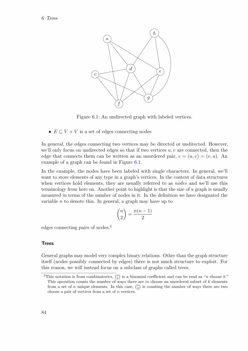
6 Trees
ab
cd e
f
g
Figure 6.1: An undirected graph with labeled vertices.
• E ⊆ V × V is a set of edges connecting nodes
In general, the edges connecting two vertices may be directed or undirected. However,we’ll only focus on undirected edges so that if two vertices u, v are connected, then theedge that connects them can be written as an unordered pair, e = (u, v) = (v, u). Anexample of a graph can be found in Figure 6.1.
In the example, the nodes have been labeled with single characters. In general, we’llwant to store elements of any type in a graph’s vertices. In the context of data structureswhen vertices hold elements, they are usually referred to as nodes and we’ll use thisterminology from here on. Another point to highlight is that the size of a graph is usuallymeasured in terms of the number of nodes in it. In the definition we have designated thevariable n to denote this. In general, a graph may have up to(
n
2
)=n(n− 1)
2
edges connecting pairs of nodes.2
Trees
General graphs may model very complex binary relations. Other than the graph structureitself (nodes possibly connected by edges) there is not much structure to exploit. Forthis reason, we will instead focus on a subclass of graphs called trees.
2This notation is from combinatorics,(nk
)is a binomial coefficient and can be read as “n choose k.”
This operation counts the number of ways there are to choose an unordered subset of k elementsfrom a set of n unique elements. In this case,
(n2
)is counting the number of ways there are two
choose a pair of vertices from a set of n vertices.
84

6.2 Definitions & Terminology
Definition 8 (Trees). A tree is an acyclic graph.
A cycle in a graph is any sequence of pairwise connected nodes that begin and end atthe same node. For example, the sequence of vertices aegcda in the graph in Figure 6.1forms a cycle. Likewise, the sequences begdb, bgdb, and cdgc also form cycles as well asmany others. A graph in which there are no cycles is referred to as an acyclic graph andhas a much simpler structure. This simplicity gives a tree several properties that can beexploited. An example of several trees can be found in Figure 6.2.
The example in Figure 6.2(d) is actually a disconnected tree in that there are severalcomponents whose nodes are not connected by any edges. Such graphs can be seen as acollection of trees and are usually called forests. Though forests are useful in modelingsome problems, we will again restrict our attention to connected trees such that there isonly one connected component.
Structural Properties
By definition, trees are acyclic which already gives them a high degree of structure.There are several related properties that follow from this structure. First, since we arerestricting attention to connected trees, it will always be the case that the number ofedges in a tree will be equal to one less than the number of vertices. That is:
Lemma 7. In any tree,|E| = n− 1
where n = |V |.
Recall that in general, graphs may have as many as O(n2) vertices. However, trees willnecessarily have fewer O(n) edges. This makes trees sparse graphs. Many graph problemsthat are hard or do not admit themselves to efficient solutions become easy or even trivialon sparse graphs and trees in particular.
Another consequence of a lack of cycles means that any two nodes in a tree will beconnected by exactly one, unique path. A path is much like a cycle except that it neednot begin/end at the same node. In Figure 6.2(a), the sequence of vertices afcgb form apath. This is, in fact, the only path connecting the vertices a and b. Furthermore, thelength of a path is defined as the number of edges on it. The aforementioned path afcgbhas length 4. Note that the length of.a path is also equal to the number of nodes in thepath minus one. In the same tree in Figure 6.2(a), afcgcfad is also technically a path,however, it traverses several edges more than once, backtracking from g. Such a path isreferred to as a non-simple path. A path that does not traverse an edge more than onceis a simple path and we will restrict our consideration to simple paths.
Lemma 8. Let T = (V,E) be a connected tree and let u, v ∈ V be two nodes in T .Then there exists exactly one single unique path connecting u, v.
85

6 Trees
ab
cd e
f
g
(a) The previous graph from Figure 6.1 withenough edges removed to make it a tree.
a
cb d
fe g
ih j
k
(b) Another tree drawn in a moreorganized manner.
a b c
d e
f
(c) Yet another little tree, hap-pier.
a
b
c
d
e
f g
h
(d) A disconnected tree with two components.
Figure 6.2: Several examples of trees. It doesn’t matter how the tree is depicted ororganized, only that it is acyclic. The final example, 6.2(d) represents adisconnected tree, called a forest.
86

6.2 Definitions & Terminology
a
d e f
c
g
b
(a) Tree rooted at a.
b
g
c
f
a
d e
(b) Tree rooted at b.
g
b c
f
a
d e
(c) Tree rooted at g.
Figure 6.3: Several possible rooted orientations for the tree from Figure 6.2(a).
Proof. First we observe that there has to be at least one path between u, v. Otherwise,if there were not, then T would not be a connected tree.
Now suppose, by way of contradiction that there exist at least two paths p and p′
connecting u, v such that p 6= p′. However, this means that we can now form a cycle.Starting at u and taking the first path p to v and then from v returning to u via p′. Sincethis forms a cycle, it contradicts the fact that we started with a tree. Thus, there cannotbe two distinct paths between two vertices.
These properties will prove useful in adapting trees as collection data structures.
Orienting Trees
To give trees even more structure, we can orient them. The first way that we’ll do thisis by rooting them. Imagine that you could take a tree (say any tree in Figure 6.2) andlift it from the page3 by grabbing a single node. Then shake the tree and let gravitydangle the remaining nodes downward. Then place the tree back onto the page. Thenode that you shook the tree from will be designated as the tree’s root and all othernodes are oriented downward. An example can be found in Figure 6.3 where we havedone this operation on the tree in Figure 6.2(a) by dangling from various nodes.
3Or screen if you will.
87

6 Trees
The alert reader and professional arborists4 alike will notice that we’ve drawn our treeswith the root at the top and its “branches” growing downward, the exact opposite of howmost real, organic trees grow. Trees in Computer Science “grow” downward because thatis how we read. Since trees will ultimately be used to store data it is easier for a humanto read them top-to-bottom, left-to-right. Of course, when represented in a computer,there is no such orientation; it is only a convention that we humans use when drawingand describing them. This convention is quite old; in fact Arthur Cayley, the originalmathematician who first studied trees drew them like this in his original paper [3].5
The vertical orientation of a trees lends itself to some obvious terminology, borrowedfrom the concept of a family tree. Let u be a tree node. The node immediately above itis called its parent. Any node(s) immediately below it are called u’s children. Likewise,all nodes on the path from u all the way back up to the root are known as u’s ancestors;u’s children and all nodes connected below them are called u’s descendants. Suppose wewere to remove all nodes in a tree except u and u’s descendant(s). The new tree wouldform a subtree rooted at u. Other tree-related terminology will be used. For example,the root of the tree will be the only node without a parent. If a node has no children, itwill be referred to as a leaf node.
Binary Trees
We can place more useful restrictions on our tree. An oriented tree such that every nodehas at most two children is a binary tree. This means that every node in a binary treemay have 0 children (a leaf), 1 child, or 2 children. We can further horizontally orientthe children in a binary tree. Since the number of children is restricted to at most 2, wecan refer to them as a left child and right child. All the identified relations in a binarytree node are depicted in Figure 6.4. Since a node may only have 1 child, using thisorientation means that it may have a left child and missing its right child, or it may havea right child and missing its left child.
A larger binary tree is depicted in Figure 6.5. In this tree, the nodes k, l, n, o, p, q, r areall leaf nodes. Many nodes have both a left and right child (b, g, j as examples) whilesome have a left child, but no right child (m, i for example) and some have a right child,but no left child (e, h for example).
Given this orientation, it is natural to define the depth of a node. Let u be a node ina binary tree with root r. The depth of u is the length of the unique path from r to u.The depth of the root, r itself is 0 by convention. The depth of a tree T itself is definedas the maximal depth (i.e. “deepest”) of any node in the tree. Thus, if a tree consistsof a single root node, its depth is zero.6. It is possible to have an empty tree (where|V | = 0) and so by convention and for consistency, the depth of an empty tree is usually
4Or dendrologists.5Specifically in part LVIII. On the Analytical Forms called Trees.–Part II in which he essentially defines
binary trees.6The author proposes to call this a seed ; let’s hope it catches on.
88
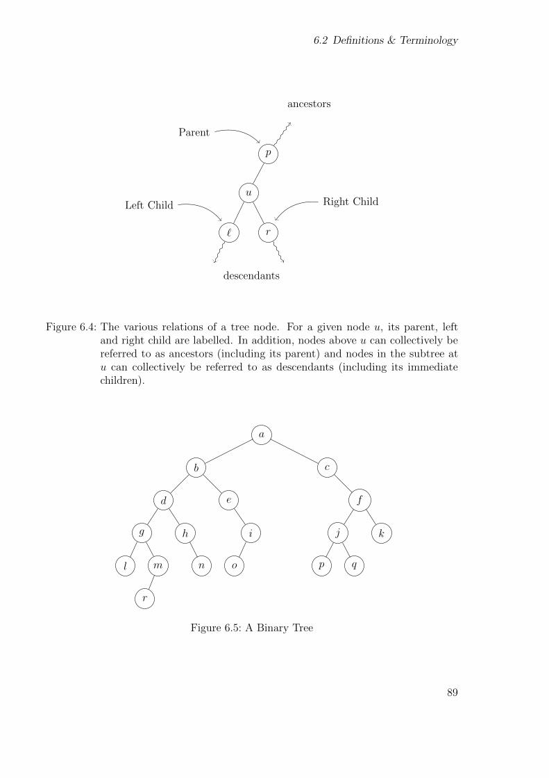
6.2 Definitions & Terminology
p
u
`
descendants
r
Left Child Right Child
Parent
ancestors
Figure 6.4: The various relations of a tree node. For a given node u, its parent, leftand right child are labelled. In addition, nodes above u can collectively bereferred to as ancestors (including its parent) and nodes in the subtree atu can collectively be referred to as descendants (including its immediatechildren).
a
b
d
g
l m
r
h
n
e
i
o
c
f
j
p q
k
Figure 6.5: A Binary Tree
89

6 Trees
Table 6.1: Depths of nodes in Figure 6.5
Node(s) Depth
a 0b, c 1d, e, f 2
g, h, i, j, k 3l,m, n, o, p, q 4
r 5
Figure 6.6: A complete tree of depth d = 3 which has 1 + 2 + 4 + 8 = 15 nodes.
−1. The depth of every node in the tree in Figure 6.5 is given in Table 6.1. Since r isthe deepest node, the depth of the tree itself is 5.
When depicting trees, we draw all nodes of equal depth on the same horizontal line. Allnodes on this line are said to be at the same level in the tree. Levels are numbered as thedepth so the root is at level 0, the next depth nodes are at level 1, etc. Structurally wecould draw the tree however we want, but placing nodes of a different depth at differentlevels makes the tree less readable.
Now, consider a complete (also called full or perfect) binary tree of depth d. That is, abinary tree in which all nodes are present at all levels; from level 0 up to level d, thedepth of the tree. How many nodes total are there in such a tree? At level 0, there wouldonly be the root. At level 1, there would be 2 children from the root. Since all nodes arepresent, at level 2, both children from the previous 2 nodes would be present giving atotal of 4, etc. That is, at each level, the number of nodes on that level doubles from theprevious level. A concrete example for d = 3 is given in Figure 6.6 which has a total of15 nodes.
We can generalize this by adding up powers of 2. At level 0, there are 20 nodes, level1, there are 21 nodes, level 2 there are 22 nodes, etc. Summing all of these nodes up to
90

6.2 Definitions & Terminology
0
Level Number of Nodes
20
1 21
2 22
3 23
4 24
......
d 2d
total
d∑i=0
i = 2d+1 − 1
Figure 6.7: A summation of nodes at each level of a complete binary tree up to depth d.
depth d gives us the following geometric series which has a well-known solution.7
n = 20 + 21 + 22 + · · ·+ 2d−1 + 2d =d∑
k=0
2k = 2d+1 − 1
This is visualized in Figure 6.7.
Taken from another perspective, if we have a complete binary tree with n nodes, itsdepth is
d = log (n+ 1)− 1
That is, the depth is logarithmic, d ∈ O(log n). This observation gives us our motivationfor using binary trees as a collection data structure. If we can develop a tree-based datastructure such that insertion, retrieval, and removal operations are all proportional to
7As a Computer Scientist, you should also find it familiar–it represents the maximum number repre-sentable by d bits.
91

6 Trees
the depth d then we have the potential for a very efficient, generalized collection datastructure. Of course it is not necessarily a simple matter as we will see shortly.
6.3 Implementation
A binary tree implementation is fairly straightforward and similar to that of a linkedlist. Each tree node is will hold references to its two children, its parent (which isoptional, but simplifies a lot of operations) and the key element stored in the tree node.In pseudocode we’ll use the same dot operator syntax as with a linked list, so that eachof these components can be referenced as follows. Let u be a tree node, then
• u.key is its key,
• u.parent is its parent,
• u.leftChild is its left child, and
• u.rightChild is its right child.
The tree itself only needs a reference to the root element, represented using T.root. Notethat we do not keep a reference to every single tree node. Keeping track of and updatingevery tree node would bring us right back to a linked list or array-based list to store allthe nodes, defeating the purpose of exploiting the tree structure. We could, however,keep track of how many nodes are in the tree as this could easily be updated with eachinsert/remove operation just as with a linked list.
As a concrete example, a pair of Java classes may be written to implement these twoobjects. In particular, the tree node class may look something like the following (getters,setters and other standard methods are omitted).
1 public class BinaryTreeNode<T>
2
3 private T key;
4 private TreeNode<T> parent;
5 private TreeNode<T> leftChild;
6 private TreeNode<T> rightChild;
7
8 ...
9
While a tree itself would look something like the following.
92

6.4 Tree Traversal
1 public class BinaryTree<T>
2
3 private TreeNode<T> root;
4 private int size;
5
6 ...
7
6.4 Tree Traversal
Before we develop the basic operations that will give us a collection data structure weneed to ensure that we have a way to process all the elements in a general binary tree.With a linked list, we could easily iterate over the elements stored in it by starting atthe head and iterating over each element until the tail. With a binary tree the order inwhich we iterate over elements is not all that clear. It is natural to start at the rootnode, but where do we go from there? To the left child or the right? If we go to the left,then we must remember to eventually come back and iterate over the right child.
More generally given a node u and its children, u.leftChild, u.rightChild in which orderdo we enumerate them? In fact, there are several tree traversal strategies each withits own advantages and applications. Each one traverses the three different nodes in adifferent order but all are based on a more general graph traversal algorithm called DFSwhich attempts to explore a graph as deeply as possible before backtracking to explorethe other areas. In general we will prefer to descend left in the tree before we backtrackand explore the right subtree. There is nothing particularly special about this preference(other than reading left-to-right is more natural). We could prefer to to right beforegoing left. However, this would be equivalent to going left while also “reversing” the tree(reversing the left/right child at each node).
To understand the traversal strategies better, we will present the traversal choices locally.At any particular node, u, we’ll refer to this node as the root (think of the subtree rootedat u) and its left and right child respectively. Given that we’ll always go left-before-right,this gives three possible orders in which to enumerate the three nodes:
• Preorder: root-left-right
• Inorder: left-root-right
• Postorder: left-right-root
Of course, any given node may be missing one or both of its children in which case wedo not enumerate it, but otherwise, we will preserve these orderings.
When we describe a traversal strategy, it is not restricted to merely enumerating all theelements in a tree. The purpose of using a binary tree as a data structure is to storedata in each of its nodes. When visiting a node, in general we can perform any operation
93

6 Trees
a
b
d e
c
f
Figure 6.8: A small binary tree.
or process on the data stored in it rather than simply enumerating the element. Thedetails of how to process a node would be specific to the type of data being stored andthe overall goal of the algorithm being executed.
6.4.1 Preorder Traversal
A preorder traversal enumerates nodes in a root-left-right manner. This means thatwe process a node immediately when we first visit it, then after processing it, we nextprocess its left child. Only after we have processed its left child and all of its descendants,do we return to process the right child and its descendants. However, we need a wayto “remember” that the right child and its subtree still need to be traversed. As a smallexample, consider the tree in Figure 6.8. Starting at the root, we enumerate a. We nextvisit its left subtree rooted at b. When we visit b, we immediately enumerate it and againtraverse left and enumerate its left child, d. Since d has no children, we backtrack to b.Having already enumerated b and its left child d, we next traverse to its right child, e.We enumerate e and since it has no children, we backtrack all the way back up to theroot a and continue to its right child, c. We immediately enumerate c, but since it hasno left child to visit, we traverse to its right child f as the final node. Altogether, theorder of enumeration was
a, b, d, e, c, f
We can implement a preorder traversal algorithm using a stack to “remember” each rightchild that we need to visit and what order to visit them. Initially, we push the tree’s rootonto the stack. We then go into a loop that executes until the stack is emptied and wehave processed all the nodes in the tree. On each iteration, we pop the node on the topof the stack and process it. We then need to process its children before we continue withother elements on the stack. To set up the next iteration, we push these child nodes ontothe stack so that they are the next ones to be processed. We need to take care to exploitthe LIFO ordering of the stack properly, however. We want the left child to be processedbefore the right child, so we push the right child first, then the left child second. The full
94

6.4 Tree Traversal
push a
(enter loop)pop, node = a
push cpush bprint a
(enter loop)pop, node = b
push epush dprint b
(enter loop)pop, node = d
push hpush gprint d
(enter loop)pop, node = g
push mpush lprint g
(enter loop)pop, node = l
(no push)(no push)
print l
(enter loop)pop, node = m
(no push)push rprint m
(enter loop)pop, node = r
(no push)(no push)
print r
(enter loop)pop, node = h
push n(no push)
print h
(enter loop)pop, node = n
(no push)(no push)
print n
(enter loop)pop, node = e
push i(no push)
print e
(enter loop)pop, node = i
(no push)push o
print i
(enter loop)pop, node = o
(no push)(no push)
print o
(enter loop)pop, node = c
push f(no push)
print c
(enter loop)pop, node = f
push kpush jprint f
(enter loop)pop, node = j
push qpush pprint j
(enter loop)pop, node = p
(no push)(no push)
print p
(enter loop)pop, node = q
(no push)(no push)
print q
(enter loop)pop, node = k
(no push)(no push)
print k
Figure 6.9: A walkthrough of a preorder traversal on the tree from Figure 6.5.
traversal is presented as Algorithm 18.
Input :A binary tree, T
Output :A preorder traversal of the nodes in T
1 S ← empty stack
2 push T.root onto S
3 while S is not empty do4 u← S.pop
5 process u
6 push u.rightChild onto S
7 push u.leftChild onto S
8 end
Algorithm 18: Stack-based Preorder Tree Traversal. If a node does not exist,we implicitly do not push it onto the stack.
A full preorder traversal on the binary tree in Figure 6.5 would result in the followingordering of vertices.
a, b, d, g, l,m, r, h, n, e, i, o, c, f, j, p, q, k
A full walkthrough of the algorithm on this example is presented in Figure 6.9.
95

6 Trees
A common alternative way of presenting a preorder traversal is to use recursion. Thisalternative version is presented as Algorithm 19. We are still implicitly using a stackto keep track of where we’ve come from in the tree, but instead of using a stack datastructure, we are exploiting the system call stack to do this.
Input :A binary tree node u
Output :A preorder traversal of the nodes in the subtree rooted at u
1 if u = null then2 return
3 else4 process u
5 preOrderTraversal(u.leftChild)
6 preOrderTraversal(u.rightChild)
7 end
Algorithm 19: preOrderTraversal(u): Recursive Preorder Tree Traversal
Applications
A preorder traversal is a straightforward and arguably the simplest to implement treetraversal strategy. As such, it is the most common traversal strategy for many applicationsthat do not require tree nodes to be traversed in any particular order. It can be used tobuild a tree, enumerate elements in a tree collection, copy a tree, etc.
TODO: more?
6.4.2 Inorder Traversal
An inorder traversal strategy visits nodes in a left-root-right order. This means thatinstead of immediately processing a node the first time we visit it, we wait until we haveprocessed its left child and all of its descendants before processing it and moving on tothe right subtree. From another we process a node when we backtrack to it (after havingprocessed the left subtree.
Again, consider the small tree in Figure 6.8. We again start at the root a, but do notimmediately enumerate it. Instead, we traverse to its left child, b. However, again wedo not enumerate b until after we have enumerated its left subtree. We traverse to dand since there is no left child, we enumerate d and return to b. Now that we haveenumerated b’s left subtree, we now enumerate b and traverse down to its right child eand enumerate it. We now backtrack all the way back up to a. Since we have enumeratedits entire left subtree, we can now enumerate a and continue to its right subtree. Since chas no left child, c is enumerated next, and then f . Altogether, the order of enumeration
96

6.4 Tree Traversal
was
d, b, e, a, c, f
We can use the same basic idea of using a stack to keep track of tree nodes, however wewant to delay processing the node until we’ve explored the left subtree. To do this, weneed a way to tell if we are visiting the node for the first time or returning from exploringthe left subtree (so that we may process it). To achieve this, we allow the node to be nullas a flag to indicate that we are backtracking from the left subtree. Thus, if the currentnode is not null, we push it back onto the stack for later processing and explore the leftsubtree. If it is null, we pop the node on the top of the stack and process it, then pushits right child to setup the next iteration. The full process is described in Algorithm 21.
Input :A binary tree, T
Output :An inorder traversal of the nodes in T
1 S ← empty stack
2 u← T.root
3 while S is not empty Or u 6= null do4 if u 6= null then5 push u onto S
6 u← u.leftChild
7 else8 u← S.pop
9 process u
10 u← u.rightChild
11 end
12 end
Algorithm 20: Stack-based Inorder Tree Traversal
In lines 6 and 10, if no such child exists, u becomes null, indicating that we are backtrackingon the next iteration.
A full inorder traversal on the binary tree in Figure 6.5 would result in the followingorder of vertices.
l, g, r,m, d, h, n, b, e, o, i, a, c, p, j, q, f, k
Again, a full walkthrough of the algorithm on this example is presented in Figure 6.10.
As with a preorder traversal, we can use recursion to implicitly use the call stack to keeptrack of the ordering. The only difference is is when we process the given node. In thepreorder case, we did it before the two recursive calls. In the inorder case, we process it
97

6 Trees
(enter loop, u = a)push a
update u = b
(enter loop, u = b)push b
update u = d
(enter loop, u = d)push d
update u = g
(enter loop, u = g)push g
update u = l
(enter loop, u = l)push l
update u = null
(enter loop,u = null)
pop l, updateu = l
process lupdate u = null
(enter loop,u = null)
pop g, updateu = g
process gupdate u = m
(enter loop, u = m)push m
update u = r
(enter loop, u = r)push r
update u = null
(enter loop,u = null)
pop r, updateu = r
process rupdate u = null
(enter loop,u = null)
pop m, updateu = m
process mupdate u = null
(enter loop,u = null)
pop d, updateu = d
process dupdate u = h
(enter loop, u = h)push h
update u = null
(enter loop,u = null)
pop h, updateu = h
process hupdate u = n
(enter loop, u = n)push n
update u = null
(enter loop,u = null)
pop n, updateu = n
process nupdate u = null
(enter loop,u = null)
pop b, updateu = b
process bupdate u = e
(enter loop, u = e)push e
update u = null
(enter loop,u = null)
pop e, updateu = e
process eupdate u = i
(enter loop, u = i)push i
update u = o
(enter loop, u = o)push o
update u = null
(enter loop,u = null)
pop o, updateu = o
process oupdate u = null
(enter loop,u = null)
pop i, updateu = i
process iupdate u = null
(enter loop,
u = null)pop i, update
u = iprocess i
update u = null
(enter loop,u = null)
pop a, updateu = a
process aupdate u = c
(enter loop, u = c)push c
update u = null
(enter loop,u = null)
pop c, updateu = c
process cupdate u = f
(enter loop, u = f)push f
update u = j
(enter loop, u = j)push j
update u = p
(enter loop, u = p)push p
update u = null
(enter loop,u = null)
pop p, updateu = p
process pupdate u = null
(enter loop,u = null)
pop j, updateu = j
process jupdate u = q
(enter loop, u = q)push q
update u = null
(enter loop,u = null)
pop q, updateu = q
process qupdate u = null
(enter loop,u = null)
pop f , updateu = f
process fupdate u = k
(enter loop, u = k)push k
update u = null
(enter loop,u = null)
pop k, updateu = k
process kupdate u = null
(done)
Figure 6.10: A walkthrough of a inorder traversal on the tree from Figure 6.5.
98

6.4 Tree Traversal
between them. The recursive version is presented as Algorithm 21.
Input :A binary tree node u
Output :An inorder traversal of the nodes in the subtree rooted at u
1 if u = null then2 return
3 else4 inOrderTraversal(u.leftChild)
5 process u
6 inOrderTraversal(u.rightChild)
7 end
Algorithm 21: inOrderTraversal(u): Recursive Inorder Tree Traversal
Applications
The primary application of an inorder tree traversal is from where it derives its name. Ifwe perform an inorder traversal on a binary search tree (see the next section), then weget an enumeration of elements that is sorted or “in order.”
TODO: more?
6.4.3 Postorder Traversal
The final depth-first-search based traversal strategy is a postorder traversal in whichnodes are visited in a left-right-root manner. That is, we hold off on processing a nodeuntil both of its children and all of their respective descendants have been processed.
We turn once again to the small binary tree in Figure 6.8. We start at the root a anddescend all the way to the left and process d since it has no children. Backtracking tob we again hold off on processing it until we’ve traversed its right child, e. Only afterwe’ve enumerated both d and e do we finally enumerate b. At this point, a’s left subtreehas been enumerated, but again we hold off on processing a until we are done with itsright subtree. c has no left child, so we enumerate its right child, f first and only thendo we process c. Finally, the last node to be processed is the root itself, a.
We can again utilize a stack data structure to perform a postorder traversal, but it getsa bit more complicated as we need to distinguish 3 different cases. When visiting a node,we need to know if it is the first time we’ve traversed it, the second time (returning fromits left subtree) or the third time (returning from its right subtree, thus it needs to beprocessed). To do this, we keep track of not only the current node but also the previousnode to know where we came from, either the parent, the left child, or the right child.
99

6 Trees
That way, we can tell if it is the first time we’ve visited the node (the previous nodewould be the parent), the second time (the previous node is the left child) or the thirdtime (the previous node is the right child). The full postorder traversal is presented inAlgorithm 22.
Input :A binary tree, T
Output :A postorder traversal of the nodes in T
1 S ← empty stack
2 prev ← null
3 push T.root onto S
4 while S is not empty do5 curr ← S.peek
6 if prev = null Or prev.leftChild = curr Or prev.rightChild = curr then7 if curr.leftChild 6= null then8 push curr.leftChild onto S
9 else if curr.rightChild 6= null then10 push curr.rightChild onto S
11 end
12 else if curr.leftChild = prev then13 if curr.rightChild 6= null then14 push curr.rightChild onto S
15 end
16 else17 process curr
18 S.pop
19 end
20 prev ← curr
21 end
Algorithm 22: Stack-based Postorder Tree Traversal
A full postorder traversal on the binary tree in Figure 6.5 would result in the followingorder of vertices.
l, r,m, g, n, h, d, o, i, e, b, p, q, j, k, f, c, a
Again, a full walkthrough of the algorithm on this example is presented in Figure 6.11.
prev = null
push a
(enter loop)update curr = (a)
check: prev = null
push (b)update prev = a
(enter loop)update curr = (b)
check:
prev.leftChild = curr((b).leftChild = (b))
push (d)update prev = b
(enter loop)
update curr = (d)check:
prev.leftChild = curr((d).leftChild = (d))
push (g)update prev = d
100

6.4 Tree Traversal
(enter loop)update curr = (g)
check:prev.leftChild = curr((g).leftChild = (g))
push (l)update prev = g
(enter loop)update curr = (l)
check:prev.leftChild = curr((l).leftChild = (l))
(noop)update prev = l
(enter loop)update curr = (l)
check:prev.rightChild = curr(null.rightChild = (l))
process lupdate prev = l
(enter loop)update curr = (g)
check:prev.rightChild = curr(null.rightChild = (g))
check:curr.leftChild = prev((l).leftChild = (l))
push (m)update prev = g
(enter loop)update curr = (m)
check:prev.rightChild = curr((m).rightChild = (m))
push (r)update prev = m
(enter loop)update curr = (r)
check:prev.leftChild = curr((r).leftChild = (r))
(noop)update prev = r
(enter loop)update curr = (r)
check:prev.rightChild = curr(null.rightChild = (r))
process rupdate prev = r
(enter loop)update curr = (m)
check:prev.rightChild = curr(null.rightChild = (m))
check:curr.leftChild = prev((r).leftChild = (r))
update prev = m
(enter loop)update curr = (m)
check:prev.rightChild = curr(null.rightChild = (m))
process mupdate prev = m
(enter loop)update curr = (g)
check:prev.rightChild = curr(null.rightChild = (g))
process gupdate prev = g
(enter loop)update curr = (d)
check:prev.rightChild = curr((m).rightChild = (d))
check:curr.leftChild = prev((g).leftChild = (g))
push (h)update prev = d
(enter loop)update curr = (h)
check:prev.rightChild = curr((h).rightChild = (h))
push (n)update prev = h
(enter loop)update curr = (n)
check:prev.rightChild = curr((n).rightChild = (n))
(noop)update prev = n
(enter loop)update curr = (n)
check:prev.rightChild = curr(null.rightChild = (n))
process nupdate prev = n
(enter loop)update curr = (h)
check:prev.rightChild = curr(null.rightChild = (h))
process hupdate prev = h
(enter loop)update curr = (d)
check:prev.rightChild = curr((n).rightChild = (d))
process dupdate prev = d
(enter loop)update curr = (b)
check:prev.rightChild = curr((h).rightChild = (b))
check:curr.leftChild = prev((d).leftChild = (d))
push (e)update prev = b
(enter loop)update curr = (e)
check:prev.rightChild = curr((e).rightChild = (e))
push (i)update prev = e
(enter loop)update curr = (i)
check:prev.rightChild = curr((i).rightChild = (i))
push (o)update prev = i
(enter loop)update curr = (o)
check:prev.leftChild = curr((o).leftChild = (o))
(noop)update prev = o
(enter loop)update curr = (o)
check:prev.rightChild = curr(null.rightChild = (o))
process oupdate prev = o
(enter loop)update curr = (i)
check:prev.rightChild = curr(null.rightChild = (i))
check:curr.leftChild = prev((o).leftChild = (o))
update prev = i
(enter loop)update curr = (i)
check:prev.rightChild = curr(null.rightChild = (i))
process iupdate prev = i
(enter loop)update curr = (e)
check:prev.rightChild = curr(null.rightChild = (e))
process eupdate prev = e
(enter loop)update curr = (b)
101

6 Trees
check:prev.rightChild = curr((i).rightChild = (b))
process bupdate prev = b
(enter loop)update curr = (a)
check:prev.rightChild = curr((e).rightChild = (a))
check:curr.leftChild = prev((b).leftChild = (b))
push (c)update prev = a
(enter loop)update curr = (c)
check:prev.rightChild = curr((c).rightChild = (c))
push (f)update prev = c
(enter loop)update curr = (f)
check:prev.rightChild = curr((f).rightChild = (f))
push (j)update prev = f
(enter loop)update curr = (j)
check:
prev.leftChild = curr((j).leftChild = (j))
push (p)update prev = j
(enter loop)update curr = (p)
check:prev.leftChild = curr((p).leftChild = (p))
(noop)update prev = p
(enter loop)update curr = (p)
check:prev.rightChild = curr(null.rightChild = (p))
process pupdate prev = p
(enter loop)update curr = (j)
check:prev.rightChild = curr(null.rightChild = (j))
check:curr.leftChild = prev((p).leftChild = (p))
push (q)update prev = j
(enter loop)update curr = (q)
check:prev.rightChild = curr
((q).rightChild = (q))(noop)
update prev = q
(enter loop)update curr = (q)
check:prev.rightChild = curr(null.rightChild = (q))
process qupdate prev = q
(enter loop)update curr = (j)
check:prev.rightChild = curr(null.rightChild = (j))
process jupdate prev = j
(enter loop)update curr = (f)
check:prev.rightChild = curr((q).rightChild = (f))
check:curr.leftChild = prev((j).leftChild = (j))
push (k)update prev = f
(enter loop)update curr = (k)
check:prev.rightChild = curr((k).rightChild = (k))
(noop)update prev = k
(enter loop)update curr = (k)
check:prev.rightChild = curr(null.rightChild = (k))
process kupdate prev = k
(enter loop)update curr = (f)
check:prev.rightChild = curr(null.rightChild = (f))
process fupdate prev = f
(enter loop)update curr = (c)
check:prev.rightChild = curr((k).rightChild = (c))
process cupdate prev = c
(enter loop)update curr = (a)
check:prev.rightChild = curr((f).rightChild = (a))
process aupdate prev = a
Figure 6.11: A walkthrough of a postorder traversal on the tree from Figure 6.5.
A recursive version would follow the same pattern as before. With a postorder traversal,we would process the node after both of the recursive calls. A recursive postorder traversal
102

6.4 Tree Traversal
is presented in Algorithm 23.
Input :A binary tree node u
Output :A postorder traversal of the nodes in the subtree rooted at u
1 if u = null then2 return
3 else4 postOrderTraversal(u.leftChild)
5 postOrderTraversal(u.rightChild)
6 process u
7 end
Algorithm 23: postOrderTraversal(u): Recursive Postorder Tree Traversal
Applications
TODO: more?
• Topological sorting
• Destroying a tree when manual memory management is necessary (roots are thelast thing that get cleaned up)
• Reverse polish notation (operand-operand-operator, unambiguous, used in old HPcalculators)
• PostScript (Page Description Language)
6.4.4 Tree Walk Traversal
It turns out that we can perform any of the three depth-first-search based tree traversalswithout using any extra space at all (that is, a stack is not necessary) by exploiting theoriented structure of a binary tree. As with the postorder traversal, we simply needto keep track of where we came from (a previous node) and where we are (a currentnode) to determine where to go next. By only keeping track of two variables, we canalso determine when a node should be processed. This traversal is generally called a“tree walk” and it is illustrated on the small tree example we’ve been using in Figure 6.12.The traversal is essentially a “walk” around the perimeter of the tree.
The rules that we follow are quite simple and only require local information. In particular,there are only three cases that we need to distinguish. Suppose we are at a node u asour current node with parent p, and left/right child as `, r respectively as in Figure 6.13.The rules are outlined in Table 6.2.
103

6 Trees
a
b
d e
c
f
Figure 6.12: A tree walk on the tree from Figure 6.8.
p
u
` r
preorder
inorder
postorder
Figure 6.13: The three general cases of when to process a node in a tree walk.
Table 6.2: Rules for Tree Walk
If previous is... Then traverse to... And process u if order is...p ` Preorder` r Inorderr p Postorder
The full tree walk is presented as Algorithm 24 and includes all three traversal strategies.The algorithm actually only keeps track of the previous node’s type (whether it was aparent, left, or right child) rather than the node itself. It is a lot more complex than thethree simple rules in Table 6.2 because we need to take care of many corner cases wherethe left and/or right children may not exist.
6.4.5 Breadth-First Search Traversal
An alternative to the depth-first-search based traversal strategies, we can explore a binarytree using what is known as a Breadth First Search (BFS) traversal. BFS is also a generalgraph traversal algorithm that explores a graph by visiting the closest vertices first before
104

6.4 Tree Traversal
Input :A binary tree, T
Output :A Tree Walk around T
1 curr ← T.root
2 prevType← parent
3 while curr 6=null do4 if prevType = parent then
//preorder: process curr here
5 if curr.leftChild exists then//Go to the left child:
6 curr ← curr.leftChild
7 prevType← parent
8 else9 curr ← curr
10 prevType← left
11 else if prevType = left then//inorder: process curr here
12 if curr.rightChild exists then//Go to the right child:
13 curr ← curr.rightChild
14 prevType← parent
15 else16 curr ← curr
17 prevType← right
18 else if prevType = right then//postorder: process curr here
19 if curr.parent = null then//root has no parent, we’re done traversing
20 curr ← curr.parent
//are we at the parent’s left or right child?
21 else if curr = curr.parent.leftChild then22 curr ← curr.parent
23 prevType← left
24 else25 curr ← curr.parent
26 prevType← right
27 end
Algorithm 24: Tree Walk based Tree Traversal
105

6 Trees
a
b
d e
c
f
Figure 6.14: A Breadth First Search Example
venturing deeper into the graph. When applied to an oriented binary tree, BFS ends upexploring a graph in a top-to-bottom, left-to-right ordering. In this manner, all nodes atthe same depth are enumerated before moving on to the next deepest level. The basicenumeration is depicted in Figure 6.14 which represents a BFS traversal on the samegraph we’ve been using in previous examples. Unsurprisingly, the order of enumerationmatches the labeling which was chosen to be top-bottom/left-right for readability.
The visualization of the ordering should give a hint as to the implementation of BFS. Ifwe were to stretch out the ordering it would be clear that the nodes are enumerated inone straight long line, suggesting a queue should be used. Indeed, we start by enqueueingthe root node. Then on each iteration, we dequeue the next node and enqueue its childrento be processed later. Since a queue is FIFO, we enqueue in the left child first. This ispresented as Algorithm 25.
Input :A binary tree, T
Output :A BFS traversal of the nodes in T
1 Q← empty queue
2 enqueue T.root into Q
3 while Q is not empty do4 u← Q.dequeue
5 process u
6 enqueue u.leftChild into Q
7 enqueue u.rightChild into Q
8 end
Algorithm 25: Queue-based BFS Tree Traversal
Contrast the BFS algorithm with the original stack-based preorder algorithm (Algorithm18). In fact, they are nearly identical. The only difference is that we use a queue insteadof a stack (and its corresponding operations) and reverse the operations on the left/rightchild. This calls back to one of the major themes of this text on the importance of“smart” data structures. Simply by changing the underlying data structure used in an
106

6.5 Binary Search Trees
algorithm, it results in a fundamentally different but complementarily useful property.
6.5 Binary Search Trees
Binary trees have a lot of structure but there is still not enough to make them efficientdata structures. As we’ve presented them so far, we can store elements and retrieve them,but without any additional ordered structure, using any one of the general traversalstrategies we’ve developed so far is still going to be O(n) in the worst case. We will nowadd some addition structure to our binary trees in order to attempt to make the generaloperations of insertion, retrieval and deletion more efficient. In particular, it will be ourgoal to make all three of these operations have complexity that is proportional to thedepth of the tree, O(d). To do that, we introduce Binary Search Trees (BSTs).
Definition 9 (Binary Search Tree). A binary search tree is a binary tree such that everynode u has an associated key, u.key which satisfies the binary search tree property :
1. Every node in the left subtree of u has a key value less than u.key
2. Every node in the right subtree of u has a key value greater than u.key
Implicitly, this definition does not allow for duplicate key values in a binary tree. Ingeneral, we could amend this definition to allow duplicate keys but we would need to beconsistent on if we place duplicates in the left or right subtree. In any case, it is not thatbig of a deal. In general, we can “break ties” using some unique value to each objects toinduce a total ordering on all elements stored in a binary search tree.8
Furthermore, though we will use integer key values in all of our examples, in practicebinary search trees need not be restricted to such values as they are intended to holdany type of object or data that we wish to store. Typically, an implementation will usea hash value of an object or data as a key value. A hash value is simply the result ofapplying a hash function that maps an object to an integer value. This is such a commonoperation it is built into many programming languages.
The binary search tree property is an inductive property. Since it holds for all nodes, itfollows that every rooted subtree in a BST is also a binary search tree. A full examplecan be found in Figure 6.15. Note that a binary search tree need not be full or completeas in the example. Many children (and thus entire subtrees) are not present. The binarysearch tree property merely guarantees that all keys in the less subtree are less and thosein the right subtree are greater than the key stored in the root respectively.
8In practice, all things being equal, we could use the memory address of two objects stored in a tree tobreak ties.
107

6 Trees
50
40
20
10
2 15
12
24
28
45
49
48
60
90
80
75 85
95
Figure 6.15: A Binary Search Tree
6.5.1 Retrieval
We can exploit the binary search tree property similar to how binary search exploits asorted array. With binary search, we check the middle element and either find what wewere search for or we have effectively cut the array in half as we know that we shouldeither search in the lower half or the upper half. Similarly, if with a binary search tree,we start a search for a particular key k at the root. If the root’s key value is greaterthan k (k < T.root.key) then we know that the key lies in its left subtree while if thesearch key value is greater (T.root.key < k) then we know that it must lie in the rightsubtree. In either case, we continue the search on the tree rooted at the left or rightchild respectively. If we ever find a node such that the key value matches we can stopthe search and return the node’s value. Of course, not every search will necessarily besuccessful. If we search for a key value that does not exist in the tree, we will eventuallyreach the end of the tree at some leaf node. If this happens, we can stop the processand return a flag indicating an unsuccessful search. Several examples are illustrated inFigure 6.16.
In some of the examples we got lucky and did not have to search too deeply in thetree. In fact, if we had searched for the key value k = 50 only a single key comparisonwould have been required. Thus, in the best case only O(1) comparisons are necessaryfor a search/retrieval operation. In the worst case, however, we had to search to thedeepest part of the tree as in the case where we successfully searched for k = 12 andunsuccessfully searched for k = 13. In both cases we made 6 key comparisons beforeending the search. In general, we may need to make d comparisons where d is the depthof the tree. This achieves what we set out to do as a retrieval operation is O(d). The full
108

6.5 Binary Search Trees
50
40
20
10
2 15
12
24
28
45
49
48
60
90
80
75 85
95
(a) Searching a BST Example 1. In this example,we search for the key value k = 45. The searchstarts at the root. Since 45 < 50 we traverse to theleft child. The next comparison finds that 40 < 45so we traverse right. Finally, the last comparisonfinds that the key value matches at which pointthe search process terminates.
50
40
20
10
2 15
12
24
28
45
49
48
60
90
80
75 85
95
(b) Searching a BST Example 2. In this example,we search for the key value k = 12. The searchstarts at the root. Since 12 < 50 we traverse tothe left child. The search then traverses left twicemore. When compared to 10, it traverses right andfinally left, finding the key value at the deepestleaf in the tree. A total of 6 comparisons wasnecessary.
50
40
20
10
2 15
12
24
28
45
49
48
60
90
80
75 85
95
(c) Searching a BST Example 3. In this example,we search for the key value k = 55 which will resultin an unsuccessful search. Starting at the root,we traverse right, then left at which point we areno longer in the tree. With only 2 comparisons,we are able to conclude and return a flag valueindicating an unsuccessful search.
50
40
20
10
2 15
12
24
28
45
49
48
60
90
80
75 85
95
(d) Searching a BST Example 4. Another unsuc-cessful search when we search for the key valuek = 13. Similar to example 6.16(b). With thesame 6 comparisons, we’ve traversed off the treeand return our flag value.
Figure 6.16: Various Search Examples on a Binary Search Tree
109
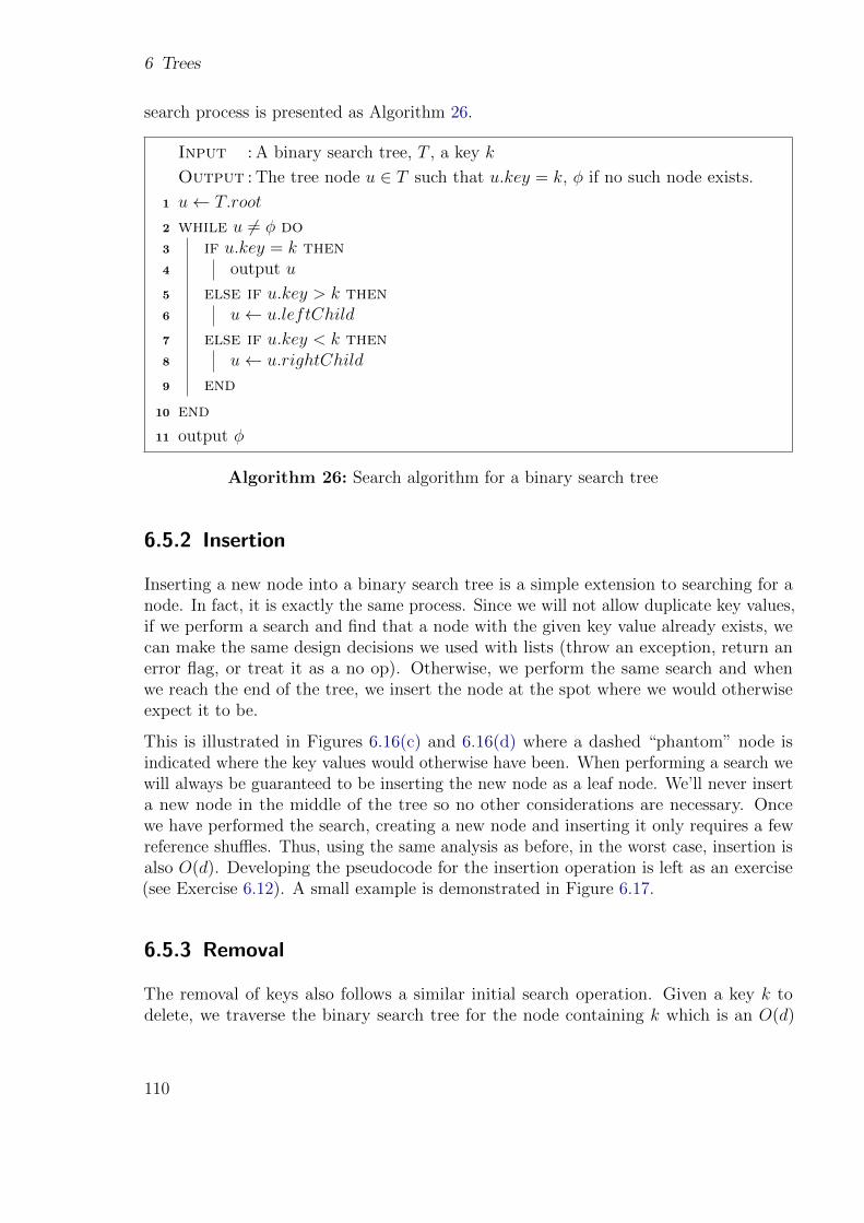
6 Trees
search process is presented as Algorithm 26.
Input :A binary search tree, T , a key k
Output :The tree node u ∈ T such that u.key = k, φ if no such node exists.
1 u← T.root
2 while u 6= φ do3 if u.key = k then4 output u
5 else if u.key > k then6 u← u.leftChild
7 else if u.key < k then8 u← u.rightChild
9 end
10 end
11 output φ
Algorithm 26: Search algorithm for a binary search tree
6.5.2 Insertion
Inserting a new node into a binary search tree is a simple extension to searching for anode. In fact, it is exactly the same process. Since we will not allow duplicate key values,if we perform a search and find that a node with the given key value already exists, wecan make the same design decisions we used with lists (throw an exception, return anerror flag, or treat it as a no op). Otherwise, we perform the same search and whenwe reach the end of the tree, we insert the node at the spot where we would otherwiseexpect it to be.
This is illustrated in Figures 6.16(c) and 6.16(d) where a dashed “phantom” node isindicated where the key values would otherwise have been. When performing a search wewill always be guaranteed to be inserting the new node as a leaf node. We’ll never inserta new node in the middle of the tree so no other considerations are necessary. Oncewe have performed the search, creating a new node and inserting it only requires a fewreference shuffles. Thus, using the same analysis as before, in the worst case, insertion isalso O(d). Developing the pseudocode for the insertion operation is left as an exercise(see Exercise 6.12). A small example is demonstrated in Figure 6.17.
6.5.3 Removal
The removal of keys also follows a similar initial search operation. Given a key k todelete, we traverse the binary search tree for the node containing k which is an O(d)
110

6.5 Binary Search Trees
15
7
4
1 5
9
30
20
17
16
23
40
Figure 6.17: Insertion of a new node into a binary search tree. A search is performed forthe key k = 16, when the open slot is found, the node is inserted.
operation. Suppose the node we wish to delete is u. There are several cases to take careof depending on how many children u has.
Case 1: Suppose that u is a leaf node and has no children. It is a simple matter todelete it by simply changing its parent node’s reference. Though we do need to check ifu is the left or right child. In particular,
• If u = u.parent.leftChild then set u.parent.leftChild← φ; otherwise
• If u = u.parent.rightChild then set u.parent.rightChild← φ.
Case 2: Suppose that u has only one child (left or right) and is missing the other child.We don’t want to “prune” the subtree of its child, but at the same time we want topreserve the binary search tree property. To do this we simply “promote” the only childup to u’s position. Specifically, suppose that u’s child is a left child. The steps to topromote it are nearly exactly the same as used to delete (circumvent) a node in a linkedlist.
If u is a left child then:
• u.parent.leftChild← u.leftChild
• u.leftChild.parent← u.parent
Otherwise if u is a right child then:
• u.parent.rightChild← u.rightChild
• u.rightChild.parent← u.parent
The operations for the case that u only has a right child is analogous. An example ofthis operation is depicted in Figures 6.18(c) and fig:bstDelete004
Case 3: Suppose that u has both of its children. Our first instinct may be to promoteone of its children up to its place similar to the previous case. In some instances thismight work. For example, consider the tree in Figure 6.15. If we wanted to delete the
111

6 Trees
root, 50, we could promote its right child, 60 up to its place. However, that is onlybecause 60 has no left child. If it had a left child (say 55), then it would not be possibleas promoting 60 up would mean it would then have to have 3 children (40, 55, 90).
There are many potential solutions to this problem, but we want to ensure that theoperation, in addition to preserving the binary search tree property, is simple, efficient,and causes a minimal change to the tree’s structure. Instead of immediately deletingthe node, let us instead remove the key, resulting in an “empty” node. We will want tobackfill this empty node with a key value in the tree that preserves the BST property.
Again, we exploit the binary search tree property. Because the subtree rooted at u is alsoa BST, every key in its left subtree is less than its key and every key in its right subtreeis greater. Thus, there are two candidates that we could “promote”: the maximum valuein the left subtree or the minimum value in the right subtree. Suppose we go with thefirst option, By replacing u with the the maximum value in the left subtree, we stillensure that all elements in the left subtree are less than it (because it was the maximumvalue) and all nodes in the right subtree are still greater than it (since it was less than uto begin with).
There are two issues that we need to deal with, however. One is finding the maximum(or minimum) value in a subtree and the other is how do we delete the node containingthe maximum value from the tree so that it can take the place of u? We’ll deal with thesecond problem first. Once we’ve found the node containing the maximum, if it has zeroor two children, we already know how to deal with that from the two previous cases.The only case we really have to deal with is if it has two children. However, we only haveto think for a moment that this is, in fact, impossible! Suppose that a node, x containedthe maximum key value and it had both children. By the binary search tree property,its right child, x.rightChild necessarily has a key value greater than i, thus x cannotcontain the maximum key value! That is, necessarily the maximum must only have atmost 1 child and we know how to deal with that situation.
How do we actually find the maximum value? Again, we exploit the binary search treeproperty. We first traverse to the left child. From there, we only have to keep traversingright until there is no longer a right child. Conversely, to find the minimum value in theright subtree, we traverse to the right child and then keep traversing left until there is no
112

6.5 Binary Search Trees
15
7
4
1 5
9
30
20
17 23
40
(a) Deletion of a node with two children(15). First step: find the maximum nodein the left-sub-tree (lesser elements).
9
7
4
1 5
30
20
17 23
40
(b) Node 15 is replaced with the ex-tremal node, preserving the BST prop-erty
9
7
4
1 5
30
20
17 23
40
(c) Deletion a node with only one child(7).
9
4
1 5
30
20
17 23
40
(d) Removal is achieved by simplypromoting the single child/subtree.
Figure 6.18: BST Deletion Operation Examples. Figures 6.18(a) and 6.18(b) depict thedeletion of a node (15) with two children. Figures 6.18(c) and 6.18(d) depictthe deletion of a node with only one child (7).
left child. The process for the former choice is presented as Algorithm 27.
Input :A node u in a binary search tree with two children.
Output :The node containing the maximum key value in u’s left subtree.
1 curr ← u.leftChildt
2 while curr.rightChild 6= φ do3 curr ← curr.rightChild
4 end
5 output curr
Algorithm 27: Finding the maximum key value in a node’s left subtree.
Examples of cases 2 and 3 can be found in Figure 6.18. The full delete operation hasinvolves several subroutines. Finding the node to be deleted (or determining it does notexist) is O(d). Finding the minimum in the left subtree is also at most O(d). Ultimately,swapping the keys and/or references is O(1). Since these are all independent operations,we have the total complexity as O(d) +O(d) +O(1) = O(d).
113

6 Trees
10
20
30
40
50
60
70
80
90
100
Figure 6.19: A degenerate binary search tree.
6.5.4 In Practice
We achieved our goal of developing a tree-based data structure that offered O(d) insert,retrieval, and update operations. However, we have still fallen short of our main goalof ensuring that these operations are all O(log n). The reason for this is that a binarysearch tree may become skewed or degenerate. Consider the binary search tree that wouldbe formed if we inserted the elements 10, 20, 30, . . . , 100 in that order. The resulting treewould look that that in Figure 6.19. This tree is degenerate because its depth is linearwith respect to the number of nodes in the tree; d = n − 1 ∈ O(n). This should lookfamiliar: a degenerate binary search tree is essentially a linked list!
In practice trees will not always be degenerate. However, there is no guarantee thatthe depth with be logarithmic. Yet more structure would be necessary to make thisguarantee. There are plenty of examples of balanced binary search trees such that insertand remove operations reorder or rebalance a tree so that for every node the left/rightsubtrees are roughly equal in depth, ensuring that d ∈ O(log n). Each one has its ownadvantages and complexity in operations such as AVL trees, 2-3/B-trees, Red-Black trees,splay trees, and treaps. We will not examine such data structures here, but know that itis possible to guarantee that the depth, and thus the basic operations are all efficient,O(log n).
Many programming languages also offer standard implementations for binary searchtrees, in particular balanced BSTs. Java, for example, provides a TreeSet (as well as aTreeMap ) which is a red-black tree implementation with guaranteed O(log n) operations.Moreover, the default iterator pattern is an inorder traversal, providing a sorted ordering.It is usually used with one of its interfaces, a SortedSet which allows you to use aComparator for ordering.
114

6.6 Heaps
6.6 Heaps
We may have fallen short of presenting a guaranteed efficient general tree data structure,however we will present a related data structure that does provide efficiency guarantees.Like stack and queues, however, this data structure’s efficiency will come at the cost ofrestricting access to its elements.
Definition 10 (Heap). A heap is a binary tree of depth d that satisfies the followingproperties.
1. It is a full up to level d− 1. That is, every node is present at every level up to andincluding level d− 1.
2. At level d all nodes are full-to-the-left. That is, all nodes at the deepest level areall as far left as possible.
3. It satisfies the heap property ; every node has a key value that is greater than bothof its children.
This definition actually defines what is referred to as a max-heap. This is because as aconsequence of the heap property, the maximum element is always guaranteed to be atthe root of the heap. Alternatively, we could redefine a heap so that every node’s childrenhas key values that are greater than it. This would define a min-heap. In practice thedistinction is unimportant and a comparator is usually used to define order. Thus, youcan get a min-heap implementation using a max-heap with a comparator that reversesthe usual ordering. A larger min-heap example can be found in Figure 6.20.
1
5
50
60
92 63
53
55
72 70
30
40
65 45
80
90 95
Figure 6.20: A min-heap
As depicted it is easy to see the fullness properties. Every node is present at every levelexcept the last one. In the deepest level, the two remaining nodes are as far left aspossible (the children of 60). Essentially there are no “gaps” in any of the levels. Thisfullness property guarantees that a heap’s depth will always be logarithmic, O(log n).
However, it is easy to see that a heap does not provide too much additional structure onthe ordering of elements other than the fact that the maximum element is at the top of
115

6 Trees
the heap. In fact, the structure of a heap resembles a real heap: it is an unorganized pileof stuff. If we were to throw something on top of a real heap, we may not have muchcontrol on where it ends up. The operations on a heap data structure are similar. Wecannot perform efficient arbitrary searches on a heap because of this lack of structure.We can, however, support two core restricted access operations. We can add elements tothe heap and we can remove the top most (getMax) element.
6.6.1 Operations
To develop the two core operations, we’ll assume that we are working with a max-heap asin Definition 10. We’ll use the smaller max-heap example in Figure 6.21 in our examples.
65
32
25
10 23
18
50
27 8
Figure 6.21: A Max-heap
Insert Key
The first operation is to insert a new key into the heap. Our first instinct may be to startat the root as we did with binary search trees. We could then move down left/right inthe heap in some manner to insert a new key, but how? Suppose we were to insert a newkey, k = 90 into the max-heap in Figure 6.21. Clearly it would need to become the newroot of the heap, displacing 65. We could continue to shove 65 down displacing either itsleft or right child. However, what criteria would we use? With only local information togo on, we may choose to exchange with the larger of the two children. Following thiscriteria we would then exchange 65 and 50, 50 and 27, resulting in something that lookslike Figure 6.22.
The problem is that this is not a valid heap as it does not fulfill the fullness property.One might be tempted to modify this approach and instead always exchange the insertednode with the lesser of the two children. This strategy would work with this particularexample, but we could easily come up with a counter example in which it fails (in fact,the same example, just swap the keys 32 and 50 and it will still fail).
Let’s take a step back and redevelop an approach that first ensures that the fullnessproperty is satisfied but the heap property need not necessarily be preserved (at first
116

6.6 Heaps
90
32
25
10 23
18
65
50
27
8
Figure 6.22: An Invalid Max-heap
at least). Preserving the fullness property means that we would necessarily insert thekey at the deepest level at the left-most available spot. For the example in Figure 6.21,this would mean inserting as the left child of 18. Inserting 90 in this manner clearlyviolates the heap heap property, however, so we need to “fix” the heap. This process isknown as heapifying. We exchange the inserted key with its parent until either 1) theheap property is satisfied or 2) we’ve reached the root node and the inserted key hasbecome the new root of the heap. This process is fully illustrated in Figure 6.23.
The heapify process is presented as Algorithm 28 which assumes that the new key hasalready been inserted in the next available spot. The algorithm makes key comparisons,continually exchanging keys until the heap property is satisfied or it reaches the root.This pseudocode, as presented, assumes a tree-based implementation.
Input :A heap H and an inserted node u
1 curr ← u
2 while curr.parent 6= φ and curr.key > curr.parent.key do3 swap curr.key, curr.parent.key
4 curr ← curr.parent
5 end
Algorithm 28: Heapify: fixing a heap data structure after the insertion of a newnode, u.
For the moment we will assume that we have an easy way to insert a node at the nextavailable spot. The heapify algorithm itself makes at most d comparisons and swapsin the worst case (as was the case in the example in Figure 6.23). If we don’t need toheapify all the way up to the root node, then even fewer comparisons and swaps wouldbe necessary, but ultimately the process is O(d). However, since a heap guaranteesthe fullness property, d = O(log n), the process only requires a logarithmic number ofcomparisons/swaps in the worst case.
117

6 Trees
65
32
25
10 23
18
90
50
27 8
(a) The new key, k = 90 is inserted at the nextavailable spot.
65
32
25
10 23
90
18
50
27 8
(b) The first comparison finds that 90 and itsparent 18 are out of order and exchanges them.
65
90
25
10 23
32
18
50
27 8
(c) The second comparison ends up exchanging90 and 32.
90
65
25
10 23
32
18
50
27 8
(d) The third and final comparison ends up pro-moting 90 up to the new root.
Figure 6.23: Insertion and Heapification.
118

6.6 Heaps
50
32
25
10 23
18
27
8
Figure 6.24: Another Invalid Heap
Retrieve Max
The other core operation is to get the maximum element. Because of the heap property,this is guaranteed to be the root element. First, we remove the key/value from theroot node (which we have immediate access to) and save it off to eventually return it.However, this leaves a gap in the tree that must be filled to preserve the fullness property.
Once again we may be tempted promote one of the root’s children to fill its place. Topreserve the heap property, we must necessary promote the larger of the two children.Of course we would have to continue down the heap as the promotion leaves another gapeventually promoting a leaf element up. This idea alone will not suffice however. Again,consider the heap from Figure 6.21. Were we to remove the root element 65 and proceedwith the operation as described we would move up 50 then 27 resulting in a “heap” as inFigure 6.24. Obviously this does not fulfill the fullness property as there is a gap (27’sleft child is missing).
As before, the solution is to prioritize the fullness property. Once we remove the rootelement, we need to backfill it with a node that will preserve the fullness property,specifically the “last” node (the rightmost node at the deepest level). Replacing the rootelement with the last node may not necessarily satisfy the heap property, but we canperform a top-down heapify process similar to what we did with the insert operation.This process is illustrated properly in Figure 6.25.
We leave the development of the algorithm and pseudocode as an exercise (see Exercise6.13). Assuming, as before, that we have easy access to the last element, then swappingit and the the root is an O(1) operation. The heapification may again require up to dcomparisons and swaps if the last element must be exchanged all the way down to thebottom of the heap. As before, since d = O(log n) this operation is O(log n).
Secondary Operations
The heap properties don’t allow us to do general operations such as arbitrary search andremove efficiently. We can achieve them using any of our tree traversal strategies, but all
119

6 Trees
32
25
10 23
18
50
27 8
(a) The root element, 65 is saved off in a tem-porarily variable.
23
32
25
10
18
50
27 8
(b) The last element, 23 replaces the root node.However, the heap property is not satisfied.
50
32
25
10
18
23
27 8
(c) The node is exchanged with the greater of thetwo children to preserve the heap property.
50
32
25
10
18
27
23 8
(d) Another exchange must take place before theheap is fixed.
Figure 6.25: Removal of the root element (getMax) and Heapification
120

6.6 Heaps
of these operations have the potential to be O(n).
However, there are algorithms in which a heap is used that may require that keys in aheap be changed (either increase or decrease their key values). A primary example iswhen a heap is used to implement a priority queue and we wish to change the priority ofan element that is already enqueued.
First, we assume that we have “free” access to the node whose key we want to change asfinding an arbitrary node is going to be O(n) as previously noted. Once we have thenode u, we can increase or decrease its key value. Suppose we increase it. Its key valuewas already greater than all of its descendants, so the heap property with respect to thesubtree rooted at u is still satisfied. However, we may have increased the key value suchit is now greater than its parent. We will need to once again, heapify and exchange keyswith its parents and ancestors until the heap property is once again satisfied. This isexactly the same process as when we inserted a new node at the bottom.
Likewise, we can support a decrease key operation. Since the key value was alreadysmaller than its parent, the heap property is unaffected with respect to u’s ancestors.In this case, however, the heap property could be violated with its children and/ordescendants. We simply exchange the key with the larger of its two children if the heapproperty is violated and continue downward in the heap just as we did with the retrieve(and remove) the maximum element. Both of.these operations are simply O(log n) asbefore.
6.6.2 Implementations
So far we have presented heaps as binary trees. It is possible to implement heaps using thesame tree nodes and structure as with binary trees, but it does present some challengesthat we’ll deal with later. Another, easier and simpler implementation, however is tocome full circle back to array-based lists.
Array-Based Implementation
Recall that the fullness property of a heap essentially means that all nodes are contiguous.It makes sense, then that we can store them in an array. In particular, we will store theroot element at index 1 (we will leave index 0 unused for this presentation though youcan easily shift all of the elements by one index if you’d rather not waste it).
Now, suppose a node u is stored at index i. Given this index, we need to locate u’sparent and left and right child. These will each be stored at:
• The left child is at index 2i
• The right child is at index 2i+ 1
• The parent is at index⌊i2
⌋
121

6 Trees
p
u
` r2i
i
2i+ 1
⌊i2
⌋
Figure 6.26: Heap Node’s Index Relations
0
–
1
65
2
32
3
50
4
25
5
18
6
27
7
8
8
10
9
23 · · ·
⌊i2
⌋p · · ·
i
u · · ·
2i
`
2i+ 1
r
Figure 6.27: An array implementation of the heap from Figure 6.21 along with thegeneralized parent, left, and right child relations.
These relations are illustrated in Figure 6.26.
A full example is presented in Figure 6.27 which implements the same small max-heapexample we’ve been using. It also demonstrates the backward and forward relationshipsto the parent and children nodes. Observe that the order in the array matches the orderfrom the tree if we were to perform a breadth first search on it (recall Figure 6.14).
A clear advantage to this implementation is that it is extremely easy and we can evenreuse an array-based list implementation. It is a simple matter to implement the heapifyalgorithms in terms of indices given the mappings above (see Exercise 6.14). Onedisadvantage is that it is costly to increase the size of the array when we need to addmore elements. However, amortized over the life of the heap and given the “savings” ina simpler implementation, this may not be that big of a deal.
Tree-Based Implementation
Though not common, you can implement a heap using the same binary tree structureusing a node with references to a parent, left child, and right child. However, to ensureefficient operation for the heapify algorithms, we necessarily have to keep track of aparent element for every node.
One problem is that we do not have obvious access to the “last” element or next available
122

6.6 Heaps
spot in the heap as we did with an array-based implementation. With an array, we couldeasily keep track of how many elements have been stored in the heap, say n. Then thelast element is necessarily at index n and the next available spot is at index n+ 1. Sincewe have random access, we can easily jump to either location to get the last element orto insert at the next available spot.
With a tree structure, however, we do not have such access. Though we keep track of theroot, it is not straightforward to also keep track of the last element (or the next availablespot). Searching for either using BFS or another tree traversal algorithm would kill ourO(log n) efficiency.
Fortunately, using a bit of mathematical analysis and exploiting the fullness property ofa heap will allow us to find either the last element or the first available spot in O(log n)time. We’ll focus on finding the first available open spot as the same technique can beused to find the last element with minor modifications.
Without loss of generality, we’ll assume that we’ve kept track of the number of nodes inthe heap, n and thus we can compute the depth,
d = blog nc
Due to the fullness property, simply knowing n and d give us a great deal of information.In particular, we know that there are
d−1∑k=0
2k = 2d − 1
nodes in the first d levels (levels 0 up to d− 1). Computing a simple difference,
m = n− (2d − 1)
tells us how many nodes are in the last (deepest) level, level d. We also know that if thelast level were full, it would have 2d nodes. This tell us whether or not the next availablespot is in the left subtree or the right subtree by making a simple comparison:
• If m < 2d
2= 2d−1 then the left subtree is not “full” at level d and so it contains the
next available spot.
• Otherwise if m ≥ 2d−1 then the left subtree is full and the right subtree mustcontain the next available spot.
In each case we can traverse down to the left or right child respectively (which ever’s treecontains the next available spot) and update both n and m (the number of elements atlevel d) and repeat this process until we’ve found the next available spot. This analysisis visualized in Figure 6.28 and the full process is presented as Algorithm 29.
It is not difficult to see that the complexity of this algorithm is O(d) = O(log n) since weiterate down the depth of the heap using simple arithmetic operations. Thus the problem
123

6 Trees
r
L
level d
R
level d
Number ofnodes at leveld ism = n− (2d − 1)
at most 2d
2at most 2d
2
d−1∑k=0
2k = 2d − 1
If m < 2d
2, the
open slot is inthe left subtree
If m ≥ 2d
2, the
open slot is inthe right subtree
Figure 6.28: Tree-based Heap Analysis. Because of the fullness property, we can determinewhich subtree (left or right) the “open” spot in a heap’s tree is by keepingtrack of the number of nodes, n. This can be inductively extended to eachsubtree until the open spot is found.
of finding the last element or the next available spot does not significantly increase thecomplexity of the heap’s core operations.
124

6.6 Heaps
Input :A tree-based heap H with n nodes
Output :The node whose child is the next available open spot in the heap
1 curr ← T.head
2 d← blog nc3 m← n
4 while curr has both children do5 if m = 2d+1 − 1 then
//remaining tree is full, traverse all the way left
6 while curr has both children do7 curr ← curr.leftChild
8 end
9 else//remaining tree is not full, determine if the next open
spot is in the left or right sub-tree
10 if m ≥ 2d
2then
//left sub-tree is full
11 d← (d− 1)
12 m← (m− 2d
2)
13 curr ← curr.rightChild
14 else//left sub-tree is not full
15 d← (d− 1)
16 m← m
17 curr ← curr.leftChild
18 end
19 end
20 end
21 output curr
Algorithm 29: Find Next Open Spot - Numerical Technique
6.6.3 Variations
As presented in Definition 10, the heaps we have been describing are sometimes referredto as binary heaps because they are based on a binary tree. There are other variations ofheaps that uses different structures and offer different properties.
For example, Binomial Heaps are heaps that are a collection of binomial trees. A
125

6 Trees
binomial tree of order k is a tree such that its children are binomial trees of orderk − 1, k − 2, . . . , 2, 1, 0 (that is, it has k children). This is an inductive definition so thatthe base case of k = 0 is a single node tree. A binomial tree of order k has 2k nodesand is of depth k. The core operations are a bit more complicated but have the samecomplexity of O(log n). The advantage of this implementation is that a merge operationof two heaps is also efficient (O(log n)).
A Fibonacci heap is a collection of trees that satisfy the heap property. However, thestructure is a lot more flexible than binary heaps or binomial heaps. The main advantageis that some of the operations to keep track of elements are delayed until they arenecessary. Thus, some operations may be quite expensive, but when looked at froman amortized analysis, the expected or average running time of the operations can beinterpreted as constant, O(1). This is similar to when we examined array-based lists.Sometimes (though not often) we may need to expand the underlying array. Thoughthis is an expensive operation, since it is not too common, when you average the runningtime of the core operations over the lifetime of the data structure, it all “evens out.” andlooks to be constant.
6.6.4 Applications
A heap is used in many algorithms as a data structure to efficiently hold elements to beprocessed. For example, several graph algorithms such as Prim’s Minimum SpanningTree or Dijkstra’s Shortest Path algorithms use heaps as their fundamental buildingblock. A heap is also used in Huffman’s Coding algorithm to efficiently compress a filewithout loss of information.
Priority Queue
From the core operations (insert and getMax) it might be obvious that a heap is anefficient way to implement a priority queue. The enqueue operation is a simple insert anda dequeue operation is always guaranteed to result in the maximum (highest priority)element. Since both operations are O(log n), this is far more efficient than a list-basedpriority queue. Note that the Java Collections library provides a heap-based priorityqueue implementation in the java.util.PriorityQueue<E> class.
Heap Sort
Suppose we have a collection of elements. Now suppose we threw them all into a heapand then, one-by-one, pulled them out using the getMax operation. As we pull them out,what order would they be in? Sorted of course! By using a sophisticated data structurelike a heap, we can greatly simplify the code to achieve a more complex data operation,
126

6.6 Heaps
sorting. This is referred to as Heap Sort and is presented as Algorithm 30.
Input :A collection of elements A = a1, . . . , anOutput :A, sorted
1 H ← empty min-heap
2 foreach a ∈ A do3 insert a into H
4 end
5 i← 1
6 while H is not empty do7 ai ← H.getMin
8 i← (i+ 1)
9 end
10 output A
Algorithm 30: Heap Sort
Examine at the code in this algorithm. It is extremely simple; we put stuff into adata structure, then we pull it out. It doesn’t get much simpler than that. The realmagic is in the data structure we used and exploited. This is a perfect illustration ofone of the themes of this book, borrowed from Eric S. Raymond [6] that “Smart datastructures and dumb code are a lot better than the other way around.” There are manysophisticated sorting algorithms (Quick Sort, Merge Sort, etc.) that use clever code(recursion, partitioning, etc.) and simple arrays. In contrast, Heap Sort uses very dumbcode: put stuff in, take stuff out and a very smart data structure. Beautiful.
Of course, this beauty is all for nothing if it is not also efficient. The complexity of theinsertion and getMin operations in Heap Sort actually changes on each iteration of thealgorithm because the data structure we’re using is growing and shrinking. Let’s firstanalyze the “put stuff in” phase (the foreach loop, lines 2–3). On the first iteration, nocomparisons or swaps are made as H is initially empty. On the second iteration wherewe insert the second element, H has size 1 and so 1 comparison (and potentially 1 swap)is made. In general on the i-th iteration, H has i− 1 elements in it, thus the insertionrequires roughly log i− 1 (the depth of the heap) comparisons and/or swaps. This is allsummarized in Table 6.3.
Thus, the total number of comparisons (or swaps) made by Heap Sort is the summationof the 4th column, or
n−1∑i=2
log i = log 2 + log 3 + · · ·+ log n− 1
Note that we start the index at i = 2, since the first iteration does not require any com-parisons. Using logarithm identities, we can further simplify and bound this summation:
127

6 Trees
Table 6.3: Analysis of Heap Sort
Iteration Size of H Depth of H Number of Comparisons
1 0 – 02 1 0 13 2 1 2...
......
...i i− 1 log (i− 1) log (i− 1)...
......
...n n− 1 log (n− 1) log (n− 1)
n−1∑i=2
log i = log (2) + log (3) + · · ·+ log (n− 1)
= log (2 · 3 · 4 · · · (n− 1))
= log ((n− 1)!)
≤ log (n!)
≤ log (nn)
= n log n
That is, the first phase is only O(n log n), matching the best case running time of QuickSort and other fast sorting algorithms. The analysis for the “take stuff out” phase issimilar, but in reverse. The size of the heap will be diminishing from n, n− 1, . . . , 1 andwill again contribute another factor of n log n. Since these are independent phases, theentire algorithm is an efficient O(n log n) sorting algorithm. Simple, efficient, elegant andbeautiful.
128

6.7 Exercises
6.7 Exercises
Exercise 6.1. Adapt and implement the Stack-Based Preorder Traversal (Algorithm18) for the Java BinaryTree<T> class.
Exercise 6.2. Adapt and implement the Stack-Based Inorder Traversal (Algorithm 21)for the Java BinaryTree<T> class.
Exercise 6.3. Adapt and implement the Stack-Based Postorder Traversal (Algorithm22) for the Java BinaryTree<T> class.
Exercise 6.4. Adapt and implement the Tree Walk Algorithm (Algorithm 24) for theJava BinaryTree<T> class.
Exercise 6.5. Let T be a binary tree of depth d. What is the maximum number ofleaves that T could have with respect to d?
Exercise 6.6. Develop an algorithm that inserts a new node into a binary tree at theshallowest available spot.
Exercise 6.7. Develop an algorithm that, given a binary tree T , counts the total numberof nodes in the tree (assume it is not kept track of as part of the data structure).
Exercise 6.8. Develop an algorithm that, given a binary tree T , counts the number ofleaves in it.
Exercise 6.9. Develop an algorithm that given a node u in a binary tree T determinesits depth.
Exercise 6.10. Develop an algorithm that given a binary tree T , computes its depth.
Exercise 6.11. Let T be a binary tree with n nodes. What is the maximum number ofleaves that T could have with respect to n? Provide an example for n = 15
Exercise 6.12. Develop an algorithm (write pseudocode) to insert a given key k into abinary search tree T .
Exercise 6.13. Develop an algorithm (write pseudocode) fix a heap after its root elementhas been removed.
Exercise 6.14. Rewrite Algorithm 28 (heapify) to work on an array instead of a treestructure.
129


Glossary
algorithm a process or method that consists of a specified step-by-step set of operations.
corner case a scenario that occurs outside of typical operating parameters or situations;an exceptional case or situation that may need to be dealt with in a unique ordifferent manner. 18
idiom in the context of software an idiom is a common code or design pattern. 12
iterator a pattern that allows a user to more easily and conveniently iterate over theelements in a collection. 15
leaky abstraction a design that exposes details and limitations of an implementationthat should otherwise be hidden through encapsulation.. 25
parameterized polymorphism a means in which you can make a piece of code (a method,class, or variable) generic so that its type can vary depending on the context inwhich the code is used. 13
queue a collection data structure that holds elements in a first-in first-out manner.
random access a mechanism by which elements in an array can be accessed by simplycomputing a memory offset of each element relative to the beginning of the array.19, 41
stack a collection data structure that holds elements in a last-in first-out manner. 29
syntactic sugar syntax in a language or program that is not absolutely necessary (thatis, the same thing can be achieved using other syntax), but may be shorter, moreconvenient, or easier to read/write. In general, such syntax makes the language“sweeter” for the humans reading and writing it. 15
131


Acronyms
ACID Atomicity, Concurrency, Isolation, Durability.
ADT Abstract Data Type. 7
AST Abstract Syntax Tree. 33
BFS Breadth First Search. 104, 106
CRUD Create-Retrieve-Update-Destroy.
DAG Directed Acyclic Graph.
DFS Depth First Search. 33, 93
DRY Don’t Repeat Yourself. 10
FIFO First-In First-Out. 33, 34, 106
JVM Java Virtual Machine. 15
LIFO Last-In First-Out. 29, 94
ORM Object-Relational Mapping.
RDMS Relational Database Management System.
SQL Structured Query Language.
133


Index
array-based lists, 8
balanced binary search trees, 114binary search tree, 107
definition, 107binary search trees
balanced binary search trees, 114binary tree, 88binomial heaps, 124
consumer producer pattern, 35
deque, 38
fibonacci heaps, 125
gauss’s formula, 43
heap sort, 125heaps, 115
binomial heaps, 124definition, 115fibonacci heaps, 125heap sort, 125
linked lists, 16lists, 7
array lists, 8linked lists, 16
object oriented programming, 3
priority queue, 38
queuepriority queue, 38
queues, 33
stacks, 29peek, 31
tree, 83binary, 88definition, 85
135


Bibliography
[1] Manindra Agrawal, Neeraj Kayal, and Nitin Saxena. PRIMES is in P. Ann. of Math,2:781–793, 2002.
[2] Paul Bachmann. Die Analytische Zahlentheorie. 1894.
[3] Arthur Cayley. On the theory of the analytical forms called trees. PhilosophicalMagazine Series 4, 13(85):172–176, 1857.
[4] Leonhard Euler. Solutio problematis ad geometriam situs pertinentis. Commentariiacademiae scientiarum Petropolitanae, 8:128–140, 1741.
[5] Donald E. Knuth. Big omicron and big omega and big theta. SIGACT News,8(2):18–24, April 1976.
[6] Eric S. Raymond. The Cathedral and the Bazaar. O’Reilly & Associates, Inc.,Sebastopol, CA, USA, 1st edition, 1999.
137