computer science configuration and deployment derivation - etd

COMPUTER SCIENCE

CONFIGURATION AND DEPLOYMENT DERIVATION STRATEGIES FOR

DISTRIBUTED REAL-TIME AND EMBEDDED SYSTEMS

BRIAN PATRICK DOUGHERTY

Dissertation under the direction of Professor Douglas C. Schmidt and Aniruddha Gokhale

Distributed real-time and embedded (DRE) systems are constructed by allocating soft-

ware tasks to hardware. This allocation, called adeployment plan, must ensure that design

constraints, such as quality of service (QoS) demands and resource requirements, are satis-

fied. Further, the financial cost and performance of these systems may differ greatly based

on software allocation decisions, auto-scaling strategy,and execution schedule.

This dissertation describes techniques for addressing thechallenges of deriving DRE

system configurations and deployments. First, we show how heuristic algorithms can be

utilized to determine system deployments that meet QoS demands and resource require-

ments. Second, we use metaheuristic algorithms to optimizesystem-wide deployment

properties. Third, we describe a Model-Driven Architecture (MDA) based methodology for

constructing a DRE system configuration modeling tool. Fourth, we demonstrate a method-

ology for evolving DRE systems as new components become available. Next, we provide

a technique for configuring virtual machine instances to create greener cloud-computing

environments. Finally, we present a metric for assessing and increasing performance gains

due to caching.

CONFIGURATION AND DEPLOYMENT DERIVATION STRATEGIES FOR

DISTRIBUTED REAL-TIME AND EMBEDDED SYSTEMS

By

Brian Patrick Dougherty

Dissertation

Submitted to the Faculty of the

Graduate School of Vanderbilt University

in partial fulfillment of the requirements

for the degree of

DOCTOR OF PHILOSOPHY

in

Computer Science

May, 2011

Nashville, Tennessee

Approved:

Professor Douglas C. Schmidt

Professor Aniruddha Gokhale

Professor Janos Sztipanovits

Professor Jules White

Professor Jeff Gray

ii

ACKNOWLEDGMENTS

I would like to thank Dr. Douglas C. Schmidt for his exceptional guidance and support

as my advisor throughout my academic career at Vanderbilt University. While Doug’s rep-

utation as a scholar is renowned in both academia and industry, he also has a remarkable

talent for teaching the research process to people like me who previously had little or no

research experience. If I can retain half of the vast knowledge that Doug has attempted

to impart to me, whether it be methodologies for writing technical papers, brainstorming

interesting, practical research ideas, or deciding the best way to “pitch” a solution to maxi-

mize impact, then I have no worries for what my future career will yield. His enthusiasm,

dedication, and seemingly inexhaustible energy supply have also been instrumental in the

completion of this process.

When Doug decided to take a temporary sabbatical from teaching, Dr. Aniruddha

Gokhale did not hesitate to take over as a temporary advisor and has done an excellent

job. Andy has been nothing short of completely supportive ofme continuing my previous

research and has provided key insights that have helped shape its development in recent

months. Andy has also been an excellent person to bounce an idea off of or crack a joke

with in a more informal setting, which has helped to mitigatethe anxiety that has accom-

panied these pursuits. I’m thankful that he accepted the invitation to serve on my defense

committee.

I must also express my gratitude to Dr. Jeff Gray and Dr. JanosSztipanovits for agree-

ing to serve on my defense committee. These men are titans in their fields and as a result

have extremely full schedules. I’m grateful that they wouldtake time away from their

pursuits to provide feedback on my research to increase its quality and credibility. Fur-

thermore, I would like to thank Dr. Sztipanovits for directing the Institute for Software

Integrated Systems and guiding it to becoming the prestigious research institution it is to-

day.

iii

Simply put, I cannot adequately express or quantify the debtI owe to Dr. Jules White

for all that he has done for my development as an academic and,more importantly, as a

person. Jules was the first person to see potential in me as a researcher and over the past

years has worked tirelessly to cultivate it, despite the varying levels of resistance I provided.

Jules has been the best mentor a student or person at my stage in their life could request,

and I’ll forever be grateful for him convincing me to stick itout until the end.

I must also acknowledge and thank Dr. Joseph Oldham of CentreCollege for starting

me down the path of computer science and teaching me the basics. The enthusiasm with

which he approached the discipline and his knack for making the material fun and interest-

ing convinced me to become an engineer. It was also through his guidance that I was able

to gain admission to Vanderbilt University and have this opportunity.

Finally, I would also like to thank my parents, Ken and Karen,and my brother, Ethan,

for supporting me throughout this process, regardless of the amount of my whining they’ve

had to endure. Their endless love and encouragement were instrumental in completing this

dissertation, regardless of their understanding of the technical concepts that comprise it.

iv

DEDICATION

This dissertation is dedicated to my parents and Dr. Jules White, for their seeminglyendless patience and unwavering support.

TABLE OF CONTENTS

ACKNOWLEDGMENTS . . . . . . . . . . . . . . . . . . . . . . . . . . . . . . . . . . . .. . . . . . . . . iii

DEDICATION . . . . . . . . . . . . . . . . . . . . . . . . . . . . . . . . . . . . . . . . .. . . . . . . . . . . . v

LIST OF FIGURES . . . . . . . . . . . . . . . . . . . . . . . . . . . . . . . . . . . . . .. . . . . . . . . . . x

Chapter

I. INTRODUCTION . . . . . . . . . . . . . . . . . . . . . . . . . . . . . . . . . . . . .. . . . . . 1

Overview of Research Challenges . . . . . . . . . . . . . . . . . . . . . . .. . . . . 2Overview of Research Approach . . . . . . . . . . . . . . . . . . . . . . . . .. . . . 3Research Contributions . . . . . . . . . . . . . . . . . . . . . . . . . . . . . .. . . . . . 6

BLITZ . . . . . . . . . . . . . . . . . . . . . . . . . . . . . . . . . . . . . . . . . . . 6ScatterD . . . . . . . . . . . . . . . . . . . . . . . . . . . . . . . . . . . . . . . . . . 7ASCENT Modeling Platform . . . . . . . . . . . . . . . . . . . . . . . . . . 7SEAR . . . . . . . . . . . . . . . . . . . . . . . . . . . . . . . . . . . . . . . . . . . . 8SCORCH . . . . . . . . . . . . . . . . . . . . . . . . . . . . . . . . . . . . . . . . . 10SMACK . . . . . . . . . . . . . . . . . . . . . . . . . . . . . . . . . . . . . . . . . . 10

Dissertation Organization . . . . . . . . . . . . . . . . . . . . . . . . . . .. . . . . . . . 11

II. RESEARCH EVOLUTION . . . . . . . . . . . . . . . . . . . . . . . . . . . . . . .. . . . . 12

DRE System Deployment Minimization . . . . . . . . . . . . . . . . . . . .. . . . 12Legacy DRE System Deployment Optimization . . . . . . . . . . . . . .. . . . 13Model-driven DRE System Configuration . . . . . . . . . . . . . . . . . .. . . . . 14Evolving Legacy DRE System Configurations . . . . . . . . . . . . . . .. . . . 15Virtual Machine Configuration Optimization . . . . . . . . . . . . .. . . . . . . 17Optimizing Processor Cache Performance . . . . . . . . . . . . . . . .. . . . . . 18

III. AUTOMATED DEPLOYMENT DERIVATION . . . . . . . . . . . . . . . . . .. . 21

Challenge Overview . . . . . . . . . . . . . . . . . . . . . . . . . . . . . . . . . .. . . . . 21Introduction . . . . . . . . . . . . . . . . . . . . . . . . . . . . . . . . . . . . . . .. . . . . . 21Challenges of Component Deployment Minimization . . . . . . . .. . . . . . 23Deployment Derivation with BLITZ . . . . . . . . . . . . . . . . . . . . . .. . . . . 23

BLITZ Bin-packing . . . . . . . . . . . . . . . . . . . . . . . . . . . . . . . . . 24Utilization Bounds . . . . . . . . . . . . . . . . . . . . . . . . . . . . . . . . . .25Co-location Constraints . . . . . . . . . . . . . . . . . . . . . . . . . . . . .. 26

Empirical Results . . . . . . . . . . . . . . . . . . . . . . . . . . . . . . . . . . .. . . . . . 26Experimental Platform . . . . . . . . . . . . . . . . . . . . . . . . . . . . . . .27Processor Minimization with Various Scheduling Bounds . . .. . 27

IV. LEGACY DEPLOYMENT OPTIMIZATION . . . . . . . . . . . . . . . . . . . .. . 29

vi

Challenge Overview . . . . . . . . . . . . . . . . . . . . . . . . . . . . . . . . . .. . . . . 29Introduction . . . . . . . . . . . . . . . . . . . . . . . . . . . . . . . . . . . . . . .. . . . . . 29Modern Embedded Flight Avionics Systems: A Case Study . . . . .. . . . 32Deployment Optimization Challenges . . . . . . . . . . . . . . . . . . .. . . . . . 34

Challenge 1: Satisfying Rate-monotonic Scheduling ConstraintsEfficiently . . . . . . . . . . . . . . . . . . . . . . . . . . . . . . . . . . 34

Challenge 2: Reducing the Complexity of Memory, Cost, andOther Resource Constraints . . . . . . . . . . . . . . . . . . . . . 35

Challenge 3: Satisfying Complex Dynamic Network Resourceand Topology Constraints . . . . . . . . . . . . . . . . . . . . . . . 35

ScatterD: A Deployment Optimization Tool to Minimize Bandwidthand Processor Resources . . . . . . . . . . . . . . . . . . . . . . . . . . . . . .. 36

Satisfying Real-time Scheduling Constraints with ScatterD . . . . 37Satisfying Resource Constraints with ScatterD . . . . . . . . . .. . . 38Minimizing Network Bandwidth and Processor Utilization with

ScatterD . . . . . . . . . . . . . . . . . . . . . . . . . . . . . . . . . . . . 38Empirical Results . . . . . . . . . . . . . . . . . . . . . . . . . . . . . . . . . . .. . . . . . 40

V. MODEL DRIVEN CONFIGURATION DERIVATION . . . . . . . . . . . . . . . 42

Challenge Overview . . . . . . . . . . . . . . . . . . . . . . . . . . . . . . . . . .. . . . . 42Introduction . . . . . . . . . . . . . . . . . . . . . . . . . . . . . . . . . . . . . . .. . . . . . 42Large-scale DRE System Configuration Challenges . . . . . . . . .. . . . . . 45

Challenge 1: Resource Interdependencies . . . . . . . . . . . . . . .. . 45Challenge 2: Component Resource Requirements Differ . . . . .. 46Challenge 3: Selecting Between Differing Levels of Service. . . 47Challenge 4: Configuration Cannot Exceed Project Budget . . .. 48Challenge 5: Exponential Configuration Space . . . . . . . . . . . .. 49

Applying MDA to Derive System Configurations . . . . . . . . . . . . .. . . 50Devising a Configuration Language . . . . . . . . . . . . . . . . . . . . . 51Implementing a Modeling Tool . . . . . . . . . . . . . . . . . . . . . . . . . 52Constructing a Metamodel . . . . . . . . . . . . . . . . . . . . . . . . . . . . 54Analyzing and Interpreting Model Instances . . . . . . . . . . . . .. . 56

Case Study . . . . . . . . . . . . . . . . . . . . . . . . . . . . . . . . . . . . . . . . . .. . . . 60Designing a MDA Configuration Language for DRE Systems . . 60

VI. AUTOMATED HARDWARE AND SOFTWARE EVOLUTION ANAL-YSIS . . . . . . . . . . . . . . . . . . . . . . . . . . . . . . . . . . . . . . . . . . . . . . .. . . . . . 68

Challenge Overview . . . . . . . . . . . . . . . . . . . . . . . . . . . . . . . . . .. . . . . 68Introduction . . . . . . . . . . . . . . . . . . . . . . . . . . . . . . . . . . . . . . .. . . . . . 68Motivating Case Study . . . . . . . . . . . . . . . . . . . . . . . . . . . . . . . .. . . . . 74Challenges of DRE System Evolution Decision Analysis . . . . .. . . . . . 76

Challenge 1: Evolving Hardware to Meet New Software Re-source Demands . . . . . . . . . . . . . . . . . . . . . . . . . . . . . . 76

vii

Challenge 2: Evolving Software to Increase Overall SystemValue . . . . . . . . . . . . . . . . . . . . . . . . . . . . . . . . . . . . . . 77

Challenge 3: Unrestricted Upgrades of Software and Hardwarein Tandem . . . . . . . . . . . . . . . . . . . . . . . . . . . . . . . . . . 78

Evolution Analysis via SEAR . . . . . . . . . . . . . . . . . . . . . . . . . . .. . . . 79Mapping Hardware Evolution Problems to MMKP . . . . . . . . . . 80Mapping Software Evolution Problems to MMKP . . . . . . . . . . . 81Hardware/Software Co-Design with ASCENT . . . . . . . . . . . . . 82

Formal Validation of Evolved DRE Systems . . . . . . . . . . . . . . . .. . . . . 83Top-Level Definition of an Evolved DRE System . . . . . . . . . . . 84Definition of Hardware Partition . . . . . . . . . . . . . . . . . . . . . . .. 84Definition of Software Partition . . . . . . . . . . . . . . . . . . . . . . .. 89Determining if a Final System Configuration is Valid . . . . . . .. 90

Empirical Results . . . . . . . . . . . . . . . . . . . . . . . . . . . . . . . . . . .. . . . . . 93Experimentation Testbed . . . . . . . . . . . . . . . . . . . . . . . . . . . . .93Hardware Evolution with Predefined Resource Consumption . .. 94Software Evolution with Predefined Resource Production . . .. . 96Unrestricted Software Evolution with Additional Hardware. . . . 96Comparison of Algorithmic Techniques . . . . . . . . . . . . . . . . . .98

VII. MODEL-DRIVEN AUTO-SCALING OF GREEN CLOUD COMPUT-ING INFRASTRUCTURE . . . . . . . . . . . . . . . . . . . . . . . . . . . . . . . . . .. . 100

Challenge Overview . . . . . . . . . . . . . . . . . . . . . . . . . . . . . . . . . .. . . . . 100Introduction . . . . . . . . . . . . . . . . . . . . . . . . . . . . . . . . . . . . . . .. . . . . . 100Challenges of Configuring Virtual Machines in Cloud Environments . . 103

Challenge 1: Capturing VM Configuration Options and Con-straints . . . . . . . . . . . . . . . . . . . . . . . . . . . . . . . . . . . . . 103

Challenge 2: Selecting VM Configurations to Guarantee Auto-scaling Speed Requirements . . . . . . . . . . . . . . . . . . . . . 104

Challenge 3: Optimizing Queue Size and Configurations toMinimize Energy Consumption and Operating Cost . . . 105

The Structure and Functionality of SCORCH . . . . . . . . . . . . . . .. . . . . 106SCORCH Cloud Configuration Models . . . . . . . . . . . . . . . . . . . 107SCORCH Configuration Demand Models . . . . . . . . . . . . . . . . . 108Runtime Model Transformation to CSP and Optimization . . . . .109Response Time Constraints and CSP Objective Function . . . . .. 111

Empirical Results . . . . . . . . . . . . . . . . . . . . . . . . . . . . . . . . . . .. . . . . . 114Experiment: VM Provisioning Techniques . . . . . . . . . . . . . . . .115Power Consumption & Cost Comparison of Techniques . . . . . . 116

VIII. PREDICTIVE PROCESSOR CACHE ANALYSIS . . . . . . . . . . . . . .. . . . 119

Challenge Overview . . . . . . . . . . . . . . . . . . . . . . . . . . . . . . . . . .. . . . . 119Introduction . . . . . . . . . . . . . . . . . . . . . . . . . . . . . . . . . . . . . . .. . . . . . 119DRE System Integration Example . . . . . . . . . . . . . . . . . . . . . . . .. . . . 122

viii

System Integration Architecture . . . . . . . . . . . . . . . . . . . . . .. . 122Runtime Integration Architecture . . . . . . . . . . . . . . . . . . . . .. . 124

Challenges of Analyzing and Optimizing Integration Architectures forCache Effects . . . . . . . . . . . . . . . . . . . . . . . . . . . . . . . . . . . . . . .125

Challenge 1: Existing Software/Hardware Specific Optimiza-tion Techniques Require System May Invalidate SafetyCertification . . . . . . . . . . . . . . . . . . . . . . . . . . . . . . . . . 126

Challenge 2: Data Sharing Characteristics of Software Compo-nents May Be Unknown . . . . . . . . . . . . . . . . . . . . . . . . 127

Challenge 3: Optimization Techniques Must Satisfy Real-timeScheduling Constraints . . . . . . . . . . . . . . . . . . . . . . . . . 128

Using SMACK to Evaluate and Adapt Integration Architectures to Im-prove Cache Performance . . . . . . . . . . . . . . . . . . . . . . . . . . . . . .129

Goal: A Cache Hit Characterization Metric for Software De-ployments . . . . . . . . . . . . . . . . . . . . . . . . . . . . . . . . . . . 129

SMACK Hypothesis . . . . . . . . . . . . . . . . . . . . . . . . . . . . . . . . . 129How Real-time Schedules can Potentially Impact Cache Hits .. 130Defining and Calculating SMACK Cache Metric . . . . . . . . . . . . 133Notation Quick Reference Guide . . . . . . . . . . . . . . . . . . . . . . . 137Applying the SMACK Metric to Increase System Performance . 138

Empirical Results . . . . . . . . . . . . . . . . . . . . . . . . . . . . . . . . . . .. . . . . . 140Experimental Platform . . . . . . . . . . . . . . . . . . . . . . . . . . . . . . .140Creation Process of Simulated Systems . . . . . . . . . . . . . . . . . .. 141Experiment 1: Variable Data Sharing . . . . . . . . . . . . . . . . . . . .142Experiment 2: Execution Schedule Manipulation . . . . . . . . . .. 144Experiment 3: Dynamic Execution Order and Data Sharing . . . .148Experiment 4: Predicting Performance with SMACK . . . . . . . . 151

IX. CONCLUDING REMARKS . . . . . . . . . . . . . . . . . . . . . . . . . . . . . . .. . . . 154

Automated Deployment Derivation . . . . . . . . . . . . . . . . . . . . . .. . . . . 154Legacy Deployment Optimization . . . . . . . . . . . . . . . . . . . . . . .. . . . . 155Model Driven Configuration Derivation . . . . . . . . . . . . . . . . . .. . . . . . 156Automated Hardware and Software Evolution Analysis . . . . . .. . . . . . 158Virtual Machine Configuration & Auto-scaling Optimization. . . . . . . . 159Predictive Processor Cache Analysis . . . . . . . . . . . . . . . . . . .. . . . . . . 160

BIBLIOGRAPHY . . . . . . . . . . . . . . . . . . . . . . . . . . . . . . . . . . . . . . .. . . . . . . . . . . 163

ix

LIST OF FIGURES

Figure Page

III.1. Deployment Plan Comparison . . . . . . . . . . . . . . . . . . . . .. . . . . . . . . . . . 27

III.2. Scheduling Bound vs Number of Processors Reduced . . .. . . . . . . . . . . . 28

IV.1. Flight Avionics Deployment Topology . . . . . . . . . . . . . .. . . . . . . . . . . . 30

IV.2. An Integrated Computing Architecture for Embedded Flight Avionics . . . 32

IV.3. ScatterD Deployment Optimization Process . . . . . . . . .. . . . . . . . . . . . . 38

IV.4. Network Bandwidth and Processor Reduction in Optimized Deployment . 41

V.1. Configuration Options of a Satellite Imaging System . . .. . . . . . . . . . . . . 46

V.2. Creation Process for a DRE System Configuration Modeling Tool . . . . . . 51

V.3. GME Model of DRE System Configuration . . . . . . . . . . . . . . . .. . . . . . 53

V.4. FCF Optimality with 10,000 Features . . . . . . . . . . . . . . . .. . . . . . . . . . . 58

V.5. AMP Workflow Diagram . . . . . . . . . . . . . . . . . . . . . . . . . . . . . .. . . . . . 61

V.6. GME Class View Metamodel of ASCENT . . . . . . . . . . . . . . . . . .. . . . . 63

VI.1. Software Evolution Progression . . . . . . . . . . . . . . . . . .. . . . . . . . . . . . . 74

VI.2. MMKP Representation of Hardware Evolution Problem . .. . . . . . . . . . . 80

VI.3. MMKP Representation of Software Evolution Problem . .. . . . . . . . . . . . 81

VI.4. MMKP Representation of Unlimited Evolution Problem .. . . . . . . . . . . . 83

VI.5. Hardware Evolution Solve Time vs Number of Sets . . . . . .. . . . . . . . . . 94

VI.6. Hardware Evolution Solution Optimality vs Number of Sets . . . . . . . . . . 95

VI.7. Software Evolution Solve Time vs Number of Sets . . . . . .. . . . . . . . . . . 95

VI.8. Software Evolution Solution Optimality vs Number of Sets . . . . . . . . . . . 96

VI.9. Unrestricted Evolution Solve Time vs Number of Sets . .. . . . . . . . . . . . . 97

x

VI.10. Unrestricted Evolution Solution Optimality vs Number of Sets . . . . . . . . 97

VI.11. LCS Solve Times vs Number of Sets . . . . . . . . . . . . . . . . . .. . . . . . . . . . 98

VI.12. M-HEU & ASCENT Solve Times vs Number of Sets . . . . . . . . .. . . . . . 98

VI.13. Comparison of Solve Times for All Experiments . . . . . .. . . . . . . . . . . . . 99

VI.14. Comparison of Optimalities for All Experiments . . . .. . . . . . . . . . . . . . . 99

VI.15. Taxonomy of Techniques . . . . . . . . . . . . . . . . . . . . . . . . .. . . . . . . . . . . 99

VII.1. Auto-scaling in a Cloud Infrastructure . . . . . . . . . . .. . . . . . . . . . . . . . . . 102

VII.2. SCORCH Model-Driven Process . . . . . . . . . . . . . . . . . . . .. . . . . . . . . . 106

VII.3. Monthly Power Consumption . . . . . . . . . . . . . . . . . . . . . .. . . . . . . . . . . 116

VII.4. Monthly Cost . . . . . . . . . . . . . . . . . . . . . . . . . . . . . . . . . .. . . . . . . . . . . 116

VII.5. Total Power Consumption . . . . . . . . . . . . . . . . . . . . . . . .. . . . . . . . . . . . 117

VII.6. Total Cost . . . . . . . . . . . . . . . . . . . . . . . . . . . . . . . . . . . .. . . . . . . . . . . . 117

VII.7. Power Consumption/Cost Reduction . . . . . . . . . . . . . . .. . . . . . . . . . . . . 117

VII.8. C02 Emissions . . . . . . . . . . . . . . . . . . . . . . . . . . . . . . . . .. . . . . . . . . . . 118

VIII.1. Example of an Integrated Avionics System . . . . . . . . .. . . . . . . . . . . . . . 122

VIII.2. Notional System Physical Architecture . . . . . . . . . .. . . . . . . . . . . . . . . . 123

VIII.3. Time & Space Partitioned System Architecture . . . . .. . . . . . . . . . . . . . . 123

VIII.4. Periodic Scheduler Interleaves Callback Execution . . . . . . . . . . . . . . . . . 124

VIII.5. Execution Interleaving inside Time Partition . . . .. . . . . . . . . . . . . . . . . . 125

VIII.6. Interleaved Execution Order is Repeatable . . . . . . .. . . . . . . . . . . . . . . . 126

VIII.7. Scheduling with Intra-Frame Transitions . . . . . . . .. . . . . . . . . . . . . . . . . 131

VIII.8. Scheduling with Extra-Frame Transition . . . . . . . . .. . . . . . . . . . . . . . . . 131

VIII.9. Processor Instructions Profiled with VTune . . . . . . .. . . . . . . . . . . . . . . . 140

VIII.10.System Creation Process . . . . . . . . . . . . . . . . . . . . . .. . . . . . . . . . . . . . . 141

xi

VIII.11.Amount of Data Shared vs Runtime. . . . . . . . . . . . . . . .. . . . . . . . . . . . . 143

VIII.12.Amount of Data Shared vs L2 Cache Misses . . . . . . . . . .. . . . . . . . . . . . 144

VIII.13.Amount of Data Shared vs L1 Cache Misses . . . . . . . . . .. . . . . . . . . . . . 145

VIII.14.Runtimes of Various Execution Schedules . . . . . . . .. . . . . . . . . . . . . . . . 146

VIII.15.Cache Contention Factor vs Overlaps . . . . . . . . . . . .. . . . . . . . . . . . . . . 146

VIII.16.Execution Schedules vs L1 Cache Misses . . . . . . . . . .. . . . . . . . . . . . . . 147

VIII.17.Execution Schedules vs L2 Cache Misses . . . . . . . . . .. . . . . . . . . . . . . . 148

VIII.18.Runtime vs Data Shared and Execution Order . . . . . . .. . . . . . . . . . . . . . 149

VIII.19.L1 Cache Misses vs Data Shared and Execution Order .. . . . . . . . . . . . . 150

VIII.20.L2 Cache Misses vs Data Shared and Execution Order .. . . . . . . . . . . . . 150

VIII.21.Smack Score vs Data Shared and Execution Order . . . .. . . . . . . . . . . . . 151

VIII.22.Percent Runtime Reduction vs Data Shared . . . . . . . .. . . . . . . . . . . . . . . 152

xii

CHAPTER I

INTRODUCTION

Distributed real-time and embedded (DRE) systems are constructed by determining an

allocation of software tasks to hardware, known as adeployment planor by configuring

commercial-off-the-shelf (COTS) components. In both cases, systems are subject to strict

resource requirements, such as memory and CPU utilization,and stringent QoS demands,

such as real-time deadlines and co-location constraints, making DRE system construction

difficult. Further, intelligently constructing DRE systems can result in significant perfor-

mance increases, reductions in financial cost and other benefits.

For example, minimizing the computing infrastructure (such as processors) in a DRE

system deployment helps reduce system size, weight, power consumption, and cost. To

support software components and applications on the computing infrastructure, the hard-

ware must provide enough processors to ensure that all applications can be scheduled with-

out missing real-time deadlines. In addition to ensuring scheduling constraints, sufficient

resources (such as memory) must be available to the software. It is hard to identify the best

way(s) of deploying software components on hardware processors to minimize computing

infrastructure and meet complex DRE constraints.

Often, it is desirable to optimize system-wide properties of DRE system deployments.

For example, a deployment that minimizes network bandwidthmay exhibit higher per-

formance and reduced power consumption. Intelligent algorithms, such as metaheuristic

techniques, can be used to refine system deployments to reduce system cost and resource

requirements, such as memory and processor utilization. Applying these algorithms to cre-

ate computer-assisted deployment optimization tools can result in substantial reductions of

processors and network bandwidth consumption requirements of legacy DRE systems.

DRE systems are also being constructed with commercial-off-the-shelf components to

1

reduce development time and effort. The configuration of these components must ensure

that real-time quality-of-service (QoS) and resource constraints are satisfied. Due to the

numerous QoS constraints that must be met, manual system configuration is hard. Model-

Driven Architecture (MDA) is a design paradigm that incorporates models to provide visual

representations of design entities. MDA shows promise for addressing many of these chal-

lenges by allowing the definition and automated enforcementof design constraints.

As DRE systems continue to become more widely utilized, system size and complexity

is also increasing. As a corollary, the design and configuration of such systems is becoming

an arduous task. Cost-effective software evolution is critical to many DRE systems. Select-

ing the lowest cost set of software components that meet DRE system resource constraints,

such as total memory and available CPU cycles, is an NP-Hard problem. Therefore, in-

telligent automated techniques must be implemented to determine cost-effective evolution

strategies in a timely manner.

Overview of Research Challenges

Several inherent complexities, such as strict resource requirements and rigid QoS de-

mands, make deriving valid DRE system deployments and configurations difficult. This

problem is exacerbated by the fact that many valid deployments and configurations may

exist that differ in terms of financial cost and performance,making some deployments and

configurations vastly superior to others. The following challenges must be overcome to

discover superior DRE system deployments and configurations:

1. Strict Resource Requirements.DRE system configurations and deployments must

adhere to strict resource constraints. If the resource requirements, such as memory

and CPU utilization, of software exceed the resource production of hardware, then

the software may fail to function or execute in an unpredictable manner.

2. QoS Guarantees. It is critical that DRE system configurations and deployments

2

ensure that rigorous QoS constraints, such as real-time deadlines, are upheld. There-

fore, for a deployment or configuration to be valid, a scheduling of software tasks

must exist that allows the software to execute without exceeding predefined real-time

deadlines.

3. Co-location Constraints. To ensure fault-tolerance and other domain-specific con-

straints, DRE systems are often subject to co-location constraints. Co-location con-

straints require that certain software tasks or componentsbe placed on the same hard-

ware while prohibiting others from occupying a common allocation.

4. Exponential Solution Space.Given a set of software and hardware, there is an expo-

nential number of different deployments or configurations that exist. Strict resource

requirements and QoS constraints, however, invalidate thevast majority of these de-

ployments, making manual derivation techniques obsolete.Due to the massive nature

of the solution space, automated exhaustive techniques fordetermining deployments

or configurations of even relatively small systems may take years to complete.

5. Variable Cost & Performance. Valid deployments and configurations may differ

greatly in terms of financial cost and performance. Therefore, techniques must be

capable of discovering solutions that not only satisfy design constraints, but also

yield high performance while carrying a low financial cost.

Overview of Research Approach

To overcome the challenges of determining valid DRE system deployments, configura-

tions and evolution strategies, we apply a combination of several heuristic algorithms (such

as bin-packing) metaheuristic algorithms (such as geneticalgorithms and particle swarm

optimization techniques), and model-driven configurationtechniques. These techniques

are utilized as described below:

1. Automated Deployment Derivationuses heuristic bin-packing to allocate software

3

tasks to hardware processors while ensuring that resource constraints, such as mem-

ory and cpu cycles, real-time deadlines, and co-location constraints are satisfied. By

defining strict space constraints of bins based on the available resources of hardware

nodes and schedulability analysis of software tasks, bin-packing can be used to de-

termine deployments that satisfy all design constraints ina timely manner.

2. Legacy Deployment Optimizationrequires that design constraints are satisfied while

also minimizing system-wide properties, such as network bandwidth utilization. This

process is difficult since the impact on network bandwidth utilization cannot be de-

termined by examining the allocation of a single software task. Metaheuristic tech-

niques, such as particle swarm optimization techniques andgenetic algorithms, can

be used in conjunction with heuristic bin-packing to discover optimized deployments

that would not be found with heuristic bin-packing alone. For example, this technique

could be applied to a legacy avionics deployment to determine if software tasks could

be allocated differently to create a deployment that consumes less network bandwidth

and carries a reduced financial cost.

3. MDA Driven DRE System Configuration techniques allow designers to model

DRE system configuration design constraints, domain-specific constrains, and fa-

cilitate the derivation of low-cost, valid configurations.For example, designers can

use model-driven tools to represent the DRE system constraints of a smart car, in-

vestigate the impact of adding a new component, such as an electronic control unit,

and automatically determine if a configuration exists that will support the additional

component.

4. Automated Hardware/Software Evolution techniques allow designers to enhance

existing DRE system configurations by adding or removing COTS components rather

than constructing costly new DRE systems from scratch, resulting in increased sys-

tem performance and lower financial costs. For example, a system designer could

4

specify a set of legacy components that are eligible for replacement and a set of

potential replacement components. Automated evolution can be used to generate a

set of replacement components and a set of components to remove that would yield

increased performance and/or reduced financial cost.

5. Automated Virtual Machine Configuration & Cloud Auto-scali ng Optimization

can reduce power consumption in cloud computing environments by using virtual-

ized computational resources to allow an application’s computational resources to

be provisioned on-demand. Auto-scaling is an important cloud computing technique

that dynamically allocates computational resources to applications to precisely match

their current loads, thereby removing resources that wouldotherwise remain idle and

waste power. Applying automated configuration strategies for minimizing operating

cost and energy consumption with auto-scaling can lead to cheaper, more energy-

efficient cloud computing environments.

6. Predictive Cache Modeling & Analysisis a technique that can aid designers in ac-

curately predicting the performance gains of DRE systems due to processor caching.

Utilizing a processor cache can greatly reduce system execution time. Several fac-

tors that vary between system implementations, such as cache size, data sharing of

software, and task execution schedule make it difficult to predict, quantify, and com-

pare the performance gains resulting from processor caching for multiple potential

system implementations. Further, using the predicted processor cache effects as a

heuristic for creating the software execution schedules, system execution time can

be reduced without violating QoS constraints, such as real-time deadlines and safety

certifications.

5

Research Contributions

As a result of these research efforts, I have generated several techniques for DRE sys-

tem configuration and performance optimization. First, we demonstrated the Bin-packing

LocalizatIon Technique for processor Minimization (BLITZ); Next we created ScatterD,

a hybrid technique for optimizing system deployments; Third, we constructed the Ascent

Modeling Platform (AMP) for modeling DRE system configurations; Fourth, we devised

the Software Evolution Analysis with Resources (SEAR) technique for evolving legacy

DRE system configurations; Next, we created the Smart Cloud Optimization for Resource

Configuration Handling (SCORCH) for reducing the energy consumption and operating

cost of cloud computing environments; Finally, we devised the System Metric for Applica-

tion Cache Knowledge (SMACK) for predicting and optimizingperformance gains due to

processor caching.

BLITZ

Research contributions:

1. We present the Bin-packing LocalizatIon Technique for processor minimiZation (BLITZ),

a deployment technique that minimizes the required number of processors, while ad-

hering to real-time scheduling, resource, and co-locationconstraints.

2. We show how this technique can be augmented with a harmonicperiod heuristic to

further reduce the number of required processors.

3. We present empirical data from applying three different deployment algorithms for

processor minimization to a flight avionics DRE system.

Conference Publications

1. Brian Dougherty, Jules White, Jaiganesh Balasubramanian, Chris Thompson, and

Douglas C. Schmidt, Deployment Automation with BLITZ, 31stInternational Con-

ference on Software Engineering, May 16-24, 2009 Vancouver, Canada.

6

ScatterD


1. We present a heuristic bin-packing technique for satisfying deployment resource and

real-time constraints.

2. We combine heuristic bin-packing with metaheuristic algorithms to create ScatterD,

a technique for optimizing system wide properties while enforcing deployment con-

straints.

3. We apply ScatterD to optimize a legacy industry flight avionics DRE system and

present empirical results of network bandwidth and processor reductions.

Journal Publications

1. Jules White, Brian Dougherty, Chris Thompson, Douglas C.Schmidt, ScatterD:

Spatial Deployment Optimization with Hybrid Heuristic / Evolutionary Algorithms,

ACM Transactions on Autonomous and Adaptive Systems Special Issue on Spatial

Computing

Submitted

1. Brian Dougherty, Jules White, Douglas C. Schmidt, Jonathan Wellons, Russell Keg-

ley, Deployment Optimization for Embedded Flight AvionicsSystems, STSC Crosstalk

(2010)

ASCENT Modeling Platform


1. We present the challenges that make manual DRE system configuration infeasible.

2. We provide an incremental methodology for constructing modeling tools to alleviate

these difficulties.

7

3. We provide a case study describing the construction of theAscent Modeling Platform

(AMP), which is a modeling tool capable of producing near-optimal DRE system

configurations.


1. Jules White, Brian Dougherty, Douglas C. Schmidt, ASCENT: An Algorithmic Tech-

nique for Designing Hardware and Software in Tandem, IEEE Transactions on Soft-

ware Engineering Special Issue on Search-based Software Engineering, December,

2009, Volume 35, Number 6

2. Jules White, Brian Dougherty, Douglas C. Schmidt, Selecting Highly Optimal Ar-

chitectural Feature Sets with Filtered Cartesian Flattening, Journal of Systems and

Software, August 2009, Volume 82, Number 8, Pages 1268-1284

Book Chapters

1. Brian Dougherty, Jules White, Douglas C. Schmidt, Model-drive Configuration of

Distributed, Real-time and Embedded Systems, Model-driven Analysis and Software

Development: Architectures and Functions, edited by JanisOsis and Erika Asnina,

IGI Global, Hershey, PA, USA 2010

SEAR


1. We present the Software Evolution Analysis with Resources (SEAR) technique that

transforms component-based DRE system evolution alternatives into multidimen-

sional multiple-choice knapsack problems.

2. We compare several techniques for solving these knapsackproblems to determine

valid, low-cost design configurations for resource constrained component-based DRE

systems.

8

3. We present a formal methodology for assessing the validity of evolved system con-

figurations.

4. We empirically evaluate the techniques to determine their applicability in the context

of common evolution scenarios.

5. Based on these findings, we present a taxonomy of the solving techniques and the

evolution scenarios that best suit each technique.


1. Jules White, Brian Dougherty, Douglas C. Schmidt, Selecting Highly Optimal Ar-

chitectural Feature Sets with Filtered Cartesian Flattening, Journal of Systems and

Software, August 2009, Volume 82, Number 8, Pages 1268-1284

2. Jules White, Brian Dougherty, Douglas C. Schmidt, ASCENT: An Algorithmic Tech-

nique for Designing Hardware and Software in Tandem, IEEE Transactions on Soft-

ware Engineering Special Issue on Search-based Software Engineering, December,

2009, Volume 35, Number 6

Conference Publications

1. Brian Dougherty, Jules White, Chris Thompson, and Douglas C. Schmidt, Automat-

ing Hardware and Software Evolution Analysis, 16th Annual IEEE International

Conference and Workshop on the Engineering of Computer Based Systems (ECBS),

April 13-16, 2009 San Francisco, CA USA.

Submitted

1. Brian Dougherty, Jules White, Douglas C. Schmidt, Automated Software and Hard-

ware Evolution Analysis for Distributed Real-time and Embedded Systems, The Cen-

tral European Journal of Computer Science, 2011.

9

SCORCH


1. We show how virtual machine configurations can be capturedin feature models.

2. We describe how these models can be transformed into constraint satisfaction prob-

lems (CSPs) for configuration and energy consumption optimization.

3. We show how these models can be transformed into constraint satisfaction problems

(CSPs) for configuration and energy consumption optimization.

4. We present a case-study showing the energy consumption/cost reduction produced

by this model-driven approach.

Submitted

1. Brian Dougherty, Jules White, Douglas C. Schmidt, Model-driven Configuration of

Green Cloud Computing Auto-scaling Infrastructure, The International Journal of

Grid Computing and eScience Special Issue on Green Computing, 2011. (revisions

requested)

SMACK


1. We present a heuristic-based scheduling technique that satisfies real-time scheduling

constraints and safety requirements while granting an average execution time reduc-

tion of 2.4%.

2. We present a case study of an industry avionics system thatmotivates the need for

cache optimizations in which code-level software modifications are prohibited.

3. We present the System Metric for Application Cache Knowledge (SMACK), a formal

methodology for quantifying the expected performance benefits of a system due to

processor caching.

10

4. We empirically evaluate the execution time, L1 cache misses and L2 cache misses of

44 simulated software systems with different data sharing characteristics and execu-

tion schedules.

5. We demonstrate the relationship between SMACK score and system performance.

6. We examine the impact of using SMACK as a heuristic to altersystem execution

schedules to reduce system execution time.

Dissertation Organization

Each research topic is separated into a chapter describing the advancements made in

each area. The remainder of this dissertation is organized as follows: Chapter III show-

cases automated deployment derivation of DRE systems; Chapter IV presents deployment

optimization techniques; Chapter V describes the creationof a modeling tool for auto-

mated DRE system configuration; Chapter VI demonstrates a methodology for automati-

cally evolving DRE systems configurations; Chapter VII presents an automated virtual ma-

chine configuration technique for reducing operating cost and energy consumption in cloud

computing environments; Chapter VIII provides a methodology for assessing and optimiz-

ing performance benefits due to processor caching for DRE systems; Finally, Chapter IX

presents concluding remarks and lessons learned.

11

CHAPTER II

RESEARCH EVOLUTION

This chapter examines existing research for optimizing DREsystem deployments and

configurations. The research is split into sections based on: minimizing the hardware nec-

essary to support a set of software components; techniques for improving legacy system

deployments; model-driven techniques for configuring DRE systems; DRE system con-

figuration evolution; optimization techniques for virtualmachine configuration; processor

cache optimization techniques for increasing system performance.

DRE System Deployment Minimization

Devising system deployments that reduce the need for excessive hardware is critical

to maximizing system value. DRE system deployment minimization examines software

component allocations and their effects on hardware requirements. This section examines

existing research methods for miinmizing system hardware requirements through intelli-

gent allocation of software components.

Deployment Minimization. Burchard et al [72] describe several techniques that use

component partitioning and bin-packing to reduce total required processors. These tech-

niques use several different heuristics based on scheduling characteristics to determine

more efficient deployment plans. This work, however, does not account for additional

resource constraints or co-location requirements. New techniques must be developed that

enforce resource constraints and co-location requirements to ensure system validity.

Task Allocation with Simulated Annealing. Tindell et al [112] investigate the use of

simulated annealing to generate deployments that optimizesystem response time. Unlike

heuristic algorithms, such as heuristic bin-packing, simulated annealing does not require

designers to specify an intelligent heuristic to determinetask allocation.

12

Instead, simulated annealing only requires that a metric isdetermined to score a poten-

tial solution. After a potential allocation is examined andscored, simulated annealing uses

an element of randomness to determine the next allocation tobe investigated. This allows

multiple executions of the algorithm to potentially determine different deployment plans.

This application of simulated annealing, however, does nottake into account resource con-

straints or co-location requirements. Therefore, this technique must be altered to ensure

that all DRE system constraints are satisfied.

Legacy DRE System Deployment Optimization

A number of prior research efforts are related to system-wide deployment optimization.

This section provides a taxonomy of these related works and examines their effectiveness

for optimizing legacy DRE system deployments. The related works are categorized based

on the type of algorithm used in the deployment process.

Multi-processor scheduling. Bin-packing algorithms have been successfully applied

to the NP-Hard problem of multi-processor scheduling [20].Multi-processor scheduling

requires finding an assignment of real-time software tasks to hardware processors, such that

no tasks miss any deadlines. A number of bin-packing modifications are used to optimize

the assignment of the tasks to use as few processors as possible [20,29,30,33,64]. The chief

issue of using these existing bin-packing algorithms for spatial deployment optimization to

minimize network bandwidth is that they focus on minimizingtotal processors used.

Kirovski et al. [60] have developed heuristic techniques for assigning tasks to proces-

sors in resource constrained systems to minimize system-wide power consumption. Their

technique optimizes a combination of variations in processor power consumption and volt-

age scaling. These techniques, however, do not account for network communication in the

power optimization process.

Hardware/software co-synthesis.Hardware/Software co-synthesis research has yielded

13

techniques for determining the number of processing units,task scheduling, and other pa-

rameters to optimize systems for power consumption while meeting hard real-time con-

straints. Dick et al. [34, 35], have used a genetic algorithmfor the co-synthesis problem.

As with other single-chip work, however, this research is directed towards systems that are

not spatially separated from one another.

Client/Server Task Partitioning for Power Optimization. Network power consump-

tion and processor power consumption have both been considered in work on partitioning

client/server tasks for mobile computing [24,71,116]. In this research, the goal is to deter-

mine how to partition tasks between a server and mobile device to minimize power drain

on the device. This work, however, is focused only on how network bandwidth and power

is saved by moving processing responsibilities between a single client and server.

Model-driven DRE System Configuration

Modeling tools can facilitate the process of DRE system configuration. The model in-

stances that are created using these modeling tools requirethat a user manually constructs

model instances. For larger model instances, this may take alarge amount of time. There-

fore, techniques are needed that facilitate model instanceconstruction from existing model

instances.

Typically, system designers wish to construct a single model instance from data spread

out over multiple model types. For example, a system designer may have a UML diagram

for describing system software architecture, excel spreadsheets listing the cost and specifi-

cations of candidate components, and a Ptolemy model providing fault tolerance require-

ments. To manually extract this information form multiple models would be laborious.

Model Management with Multi-Modeling Tools Multi-modeling tools are applica-

tions that allow the manipulation of multiple PSMs defined bydifferent metamodels. Multi-

modeling tools could allow the automated aggregation of data from models of different

types. In future work the use of multi-models to collect reliability, fault-tolerance, and

14

performance data from multiple disparate models will be investigated and applied to the

evaluation of model instances of DRE system configurations.

The migration of a model instance defined by a certain metamodel to a model instance

defined by a different metamodel is known as a model transformation. Since these meta-

models define different rules for constructing PSMs, the semantic meaning of the model

that is migrated can be partially or entirely lost, resulting in an incomplete transforma-

tion. In future work, procedures to transform models while minimizing data loss will be

researched.

Using these techniques, models that contain additional system configuration data, such

as Ptolemy models, could be transformed into model instances that can be used in concert

with AMP [38]. The Lockheed Martin Corporation is currentlyconstructing NAOMI [32],

a multi-modeling environment that can be utilized to aggregate data from multiple models

of different types and perform complex multi-model transformations.

Evolving Legacy DRE System Configurations

The myriad of DRE system constraints, tightly coupled hardware and software resource

requirements, and plentiful configuration options makes evolving legacy DRE system con-

figurations difficult. This section examines the use of (1) feature models for software

product-lines, (2) architecture reconfigurations to satisfy multiple resource constraints, and

(3) resource planning in enterprise organizations to facilitate upgrades to determine if their

application can mitigate these difficulties.

Automated Software Product-line Configuration. Software product-lines (SPLs)

model a system as a set of common and variable parts. A common approach to captur-

ing commonality and variability in SPLs is to use a feature model [54], which describes

the points of variability using a tree-like structure. A number of automated techniques have

been developed that model feature model configuration and evolution problems as con-

straint satisfaction problems [12] or SAT solvers to Benavides et al. [12,121], satisfiability

15

problems [78], or propositional logic problems [9]. Although these techniques work well

for automated configuration of feature models, they have typically not been applied with

resource constraints, since they use exponential worst-case search techniques.

Architectural considerations of embedded systems.Many hardware/software co-

design techniques can be used to analyze the effectiveness of embedded system archi-

tectures. Slomka et al [104] discuss the development life cycle of designing embedded

systems. In their approach, various partitionings of software onto hardware devices are

proposed and analyzed to determine if predefined performance requirements can be met. If

the performance goals are not attained, the architecture ofthe system will be modified by

altering the placement of certain devices in the architecture. Even if a valid configuration

is determined, it may still be possible to optimize the performance by moving devices.

However, these optimizations are achieved by altering the system architecture, which

may not be always desirable or possible. Architectural hardware/software co-design deci-

sions traditionally do not consider comparative resource constraints or financial cost opti-

mization.

Maintenance models for enterprise organizations.The difficulty of software evolu-

tion is a common and significant obstacle in business organizations. Ng et al [85] discuss

the impact of vendor choice and hardware consumption to showthe sizable financial and

functional impact that results from installingenterprise resource planning(ERP) software.

Other factors related to calculating evolution costs include vendor technical support, the

difficulty of replacing the previous version of the software, and annual maintenance costs.

Maintenance models are used to predict and plan the effect ofpurchasing and utilizing

various software options on overall system value. Steps forthe creating maintenance mod-

els with increased accuracy for describing the ramifications of an ERP decision are also

presented.

Currently, maintenance models require a substantial amount of effort to calculate the

overall impact of installing a single software package, much of which can not be done

16

through computation. While maintenance models can be used to assess the value of the

functionality and durability added by a certain software package, they have not been used

to explore the hardware/software co-design space to determine valid configurations from

large sets of potential hardware devices and software components. Instead, they are used

to define a process for analyzing and calculating the value ofpredefined upgrades.

Virtual Machine Configuration Optimization

Optimizing system configurations can also yield great performance benefits in other

computing environments, such as cloud computing infrastructures. This section examines

techinques that can be applied to virtual machine configuration to increase system perfor-

mance.

VM forking handles increased workloads by replicating VM instances onto new hosts

in negligible time, while maintaining the configuration options and state of the original

VM instance. Cavilla et al. [63] describe SnowFlock, which uses virtual machine forking

to generate replicas that run on hundreds of other hosts in a less than a second. This

replication method maintains both the configuration and state of the cloned machine. Since

SnowFlock was designed to instantiate replicas on multiplephysical machines, it is ideal

for handling increased workload in a cloud computing environment where large amounts

of additional hardware is available.

SnowFlock is effective for cloning VM instances so that the new instances have the

same configuration and state of the original instance. As a result, the configuration and

boot time of a VM instance replica can be almost entirely bypassed. This technique, how-

ever, requires that at least a single virtual machine instance matching the configuration

requirements of the requesting application is booted.

Automated feature derivation. To maintain the service-level agreements provided by

cloud computing environments, it is critical that techniques for deriving VM instance con-

figurations are automated since manual techniques cannot support the dynamic scalability

17

that makes cloud computing environments attractive. Many techniques [13,118–120] exist

to automatically derive feature sets from feature models. These techniques convert feature

models to CSPs that can be solved using commercial CSP solvers. By representing the

configuration options of VM instances as feature models, these techniques can be applied

to yield feature sets that meet the configuration requirements of an application. Existing

techniques, however, focus on meeting configuration requirements of one application at a

time. These techniques could therefore be effective for determining an exact configuration

match for a single application.

Optimizing Processor Cache Performance

DRE system performance can be vastly increased by effectively utilizing processor

caching. This section examines the impact of (1) software cache optimization techniques,

(2) hardware cache optimization techniques, and (3) other DRE system performance opti-

mization techniques on the effectiveness of processor caching.

Software Cache Optimization Techniques. Many techniques exist to increase the

effectiveness of processor caches by altering software at the code level to change the order

in which data is accessed. These optimizations, known as data access optimizations [61],

focus on changing the manner in which loops are executed. Onetechnique, known as Loop

Interchange, can be used to reorder multiple loops such thatthe data access of common

elements in respect to time, referred to astemporal localityis maximized [4,102,123,124].

Another technique, referred to as loop fusion, is often thenapplied to further increase

cache effectiveness. Loop fusion is the process of merging multiple loops into a single

loop and altering data access order to maximize temporal locality [17, 58, 103, 114]. Yet

another technique for improving the cache effectiveness ofsoftware is to utilizeprefetch

instructions. A prefetch instruction is retrieves data from memory and writes to the cache

before the data is requested by the application [61]. Prefetch instructions can be inserted

18

manually into software at the code level and have been shown to reduce memory latency

and/or cache miss rate [25,41].

While these techniques have all been shown to increase the effectiveness of software

utilizing processor caches, they all require code-level optimizations of the software. Many

systems are safety critical and must be comprised of safety-critical components. Any alter-

ation to these components can introduce unforeseen side effects and invalidate the safety

certification. Further, developers may not have code-levelproprietary components that are

purchased. These restrictions prohibit the use of any code-level modifications, such as those

used in loop fusion and loop interchange, as well as manuallyadding prefetch instructions.

Hardware Cache Optimization Techniques.Several techniques also exist for alter-

ing systems at the hardware level to increase the effectiveness of processor caches. One

technique is to alter thecache replacement policythat is used by the processor to determine

which line of cache is replaced when new data is written to thecache. Several policies

exist, such as Least Recently Used (LRU), Least Frequently Used (LRU), First In First Out

(FIFO), and random replacement [2,45,46].

Which policy is used can substantially influence the performance of a system. For

example, LRU is effective for systems in which the same data is likely to be accessed

again before enough data has been written to the cache to completely overwrite the cache.

However, if enough new data is written to the cache that previously cached data is always

overwritten before it can be accessed then performance gains will be minimal. In these

cases, a random replacement policy will probably yield increased cache effectiveness.

Further, certain policies are shown to work better for different cache levels [2], with

LRU performing well for L1 cache levels, but not as well for large data sets that may

completely exhaust the cache. Unfortunately, it is very difficult and often impossible to

alter the cache policy of existing hardware. Therefore, cache replacement policies should

be taken into account when choosing hardware so that the effects of cache optimizations

made at the software or execution schedule level will be maximized.

19

DRE System Configuration Optimization. While techniques such heuristic-based

scheduling with SMACK can be applied to increase the processor cache effects of existing

systems, other techniques focus on increasing performancethrough intelligent system con-

struction. Constructing valid DRE system implementationsby configuring prefabricated

COTS components is non-trivial due to several constraints,such as real-time requirements,

budgetary limitations, and strict resource constraints. However, substantial reductions in

execution time, financial cost, and resource requirements can be realized by intelligently

configuring DRE systems [37,37].

Other techniques, such as Software Product Lines (SPLs), examine points of variability

in the hardware and software of the system to determine if certain variants offer superior

performance [12, 121]. These techniques are appropriate for constructing new system im-

plementations or evolving existing system implementations so that all DRE constraints are

met. However, these techniques do nothing to further optimize system performance after a

valid configuration has been determined.

20

CHAPTER III

AUTOMATED DEPLOYMENT DERIVATION

Challenge Overview

This chapter provides motivation for automated deploymentderivation techniques to

determine valid DRE system deployments. We introduce a heuristic technique for pro-

cessor minimization of a legacy flight avionics system. We show how the application of

this technique can substantially reduce the hardware requirements and cost of deployments

while satisfying additional DRE system constraints.

Introduction

Software engineers who develop distributed real-time and embedded (DRE) systems

must carefully map software components to hardware. These software components must

adhere to complex constraints, such as real-time scheduling deadlines and memory limita-

tions, that are hard to manage when planning deployments that map the software compo-

nents to hardware [10]. How software engineers choose to mapsoftware to hardware has a

direct impact on the number of processors required to implement a system.

Ideally, software components for DRE systems should be deployed on as few processors

as possible. Each additional processor used by a deploymentadds size, weight, power

consumption, and cost to the system [81]. For example, it hasbeen estimated that each

additional pound of computing infrastructure on a commercial aircraft results in a yearly

loss of $200 per aircraft in fuel costs [109]. Likewise, eachpound of processor(s) requires

four additional pounds of cooling, power supply, and other support hardware. Naturally,

reducing fuel consumption also reduces emissions, benefiting the environment [109].

Several types of constraints must be considered when determining a validdeployment

21

plan, which allocates software components to processors. First, software components de-

ployed on each processor must not require more resources, such as memory, than the pro-

cessor provides. Second, some components may have co-location constraints, requiring

that one component be placed on the same processor as anothercomponent. Moreover, all

components on a processor must be schedulable to assure theymeet critical deadlines [98].

Existing automated deployment techniques [16,20,65] leveraged by software engineers

do not handle all these constraints simultaneously. For example, Rate Monotonic First-Fit

Scheduling [16] can guarantee real-time scheduling constraints, but does not guarantee

memory constraints or allow for forced co-location of components. Co-location of com-

ponents is a critical requirement in many DRE systems. Moreover, if deploying a set of

components on a processor results in CPU over-utilization,critical tasks performed by a

software component may not complete by their deadline, which may be catastrophic. DRE

software engineers must therefore identify deployments that meet these myriad constraints

andminimize the total number of processors [33].

We provide three contributions to the study of software component deployment opti-

mizations for DRE systems that address the challenges outlined above.

1. We present theBin packing LocatIon Technique for processor minimiZation(BLITZ),

which uses bin packing to allocate software applications toa minimal number of pro-

cessors and ensure that real-time scheduling, resource, and co-location constraints

are simultaneously met.

2. We describe a case study that motivates the minimization of processors in a produc-

tion flight avionics DRE system.

3. We present empirical comparisons of minimizing processors for deployments with

BLITZ for three different scheduling heuristics versus thesimple bin-packing of one

component per processor used in the avionics case study.

22

Challenges of Component Deployment Minimization

This section summarizes the challenges of determining a software component deploy-

ment that minimizes the number of processors in a DRE system.

Rate-monotonic scheduling constraints. To create a valid deployment, the mapping

of software components to processors must guarantee that none of the software compo-

nents’ tasks misses its deadline. Even if rate monotonic scheduling is used, a series of

components that collectively utilize less than 100% of a processor may not be schedula-

ble. It has been shown that determining a deployment of multiple software components to

multiple processors that will always meet real-time scheduling constraints is NP-Hard [20].

Task co-location constraints. In some cases, software components must be co-located

on the same processor. For example, variable latency of communication between two com-

ponents on separate processors may prevent real-time constraints from being honored. As

a result, some components may require co-location on the same processor, which precludes

the use of bin-packing algorithms that treat each software component to deploy as a sepa-

rate entity.

Resource constraints. To create a validate deployment, each processor must provide

the resources (such as memory) necessary for the set of software components it supports to

function. Developers must ensure that components deployedto a processor do not consume

more resources than are present. If each processor does not provide a sufficient amount

of these resources to support all tasks on the processor, a task will not be able execute,

resulting in a failure.

Deployment Derivation with BLITZ

TheBinpacking LocalizatIon Technique for processor minimiZation (BLITZ) is a first-

fit decreasing bin-packing algorithm we developed to (1) assign processor utilization values

that ensure schedulability if not exceeded and (2) enhance existing techniques by ensuring

that multiple resource and co-location constraints are simultaneously honored.

23

BLITZ Bin-packing

The goal of a bin packer is to place a set of items into a minimalset of bins. Each item

takes up a certain amount of space and each bin has a limited amount of space available

for packing. An item can be placed in a bin as long as its placement does not exceed

the remaining space in the bin. Multi-dimensional bin packing extends the algorithm by

adding extra dimensions to bins and items (e.g., length, width, and height) to account for

additional requirements of items. For example, an item may have height corresponding to

its CPU utilization and width corresponding to consumed memory.

BLITZ uses an enhanced multi-dimensional bin packing algorithm to generate valid

deployments that honor multiple resource constraints and co-location constraints as well as

the standard real-time scheduling constraints. In BLITZ, each processor is modeled as a

bin and each independent component or co-located group of components is modeled as an

item. Each bin has a dimension corresponding to the available CPU utilization. Each item

has a dimension that represents the CPU utilization it requires, as well as a a dimension cor-

responding to each resource, such as memory, that it consumes. Each bin’s size dimension

corresponding to available CPU utilization is initialized100%. The resource dimensions

are set to the amount of each resource that the processor offers.

To pack the items, they are first sorted in decreasing order ofutilization. Next, BLITZ

attempts to place the first item in the first bin. If the placement of the item does not exceed

the size of the bin (available resources and utilization) ofthe bin (processor), the item is

placed in the bin. The dimensions of the items are then subtracted from the dimensions of

the bin to reflect the addition. If the item does not fit, BLITZ attempts to insert the item

into the next bin. This step is repeated until all items are packed into bins or no bin exists

that can contain the item.

Burchard et al [72] describe several techniques that use component partitioning and

bin-packing to reduce total required processors. This work, however, does not account

for additional resource constraints, such as memory. Furthermore, these techniques do not

24

allow for co-location constraints that require specific components to reside on the same

processor.

Utilization Bounds

Conventional bin-packing algorithms assume that each bin has a static series of dimen-

sions corresponding to available resources. For example, the amount of RAM provided

by the processor is constant. Applying conventional bin-packing algorithms to software

component deployment is a challenge since it is hard to set a static bin dimension that

guarantees the components are schedulable. Scheduling canonly be modeled with a con-

stant bin dimension of utilization if a worst-case scheduling of the system is assumed. Liu-

Layland [74] have shown that a fixed bin dimension of 69.4% will guarantee schedulability

but in many cases, tasks can have a higher utilization and still be schedulable.

The Liu-Layland equation states that the maximum processorutilization that guarantees

schedulability is equal to 21/x−1, where x is the total number of components allocated to

the processor. With BLITZ, each bin has a scheduling dimension that is determined by the

Liu-Layland equation and the number of components currently assigned to the bin. Each

item will represent at least one but possibly multiple co-located components. Each time an

item is assigned to a bin, BLITZ uses the Liu-Layland formulato dynamically resize the

bin’s scheduling dimension according to the number of components held by the items in

the bin.

If the frequency of execution, or periodicity, of the components’ execution require-

ments is known, higher processor utilization above the Liu-Layland bound is also possible.

Components with harmonic periods (e.g., periods that can be repeatedly doubled or halved

to equal each other) can be allocated to the same processor with schedulability ensured, as

long as the total utilization is less than or equal to 100%.

Unlike other deployment algorithms [31, 72], BLITZ uses multi-stage packing to ex-

ploit harmonic periods. In the first stage, components with harmonic periods are grouped

25

together. In each successive stage, the components from thegroup with the largest aggre-

gate processor utilization are deployed to the processors using a first-fit packing scheme.

If not all periods of the components in a bin are harmonic (multiples of one another), an

item is allocated to a bin only if the utilization of its components fits within the dynamic

scheduling Liu-Layland dimension and all other resource dimensions. If all component

periods within a bin are harmonic, the utilization dimension is not dynamically calculated

with Liu-Layland and a fixed value of 100% is used.

Co-location Constraints

To allow for component co-location constraints, BLITZ groups components that require

co-location into a single item. Each item has utilization and resource consumption equal

to that of the component(s) it represents. Each item remembers the components associ-

ated with it. The Liu-Layland and harmonic calculations areperformed on the individual

components associated with the items in a bin and not each item as a whole.

Empirical Results

This section presents the results of applying BLITZ to a flight avionics case study pro-

vided by Lockheed Martin Aeronautics through the SPRUCE portal (www.sprucecommunity.

org), which provides a web-accessible tool that pairs academicresearchers with industry

challenge problems complete with representative project data. This case study comprised

14 processors, 89 total components, and 14 co-location constraints. We compared 2 differ-

ent bin-packing strategies against both BLITZ and the baseline deployment of this avionics

system, produced by the original avionics domain experts.

Experimental Platform

All algorithms were implemented in Java and all experimentswere conducted on an

Apple MacbookPro with a 2.4 GHz Intel Core 2 Duo processor, 2 gigabytes of RAM,

26

running OS X version 10.5.5, and a 1.6 Java Virtual Machine (JVM) run in client mode.

All experiments required less than 1 second to complete witheach algorithm.

Processor Minimization with Various Scheduling Bounds

This experiment compared the following bin-packing strategies against BLITZ and

the baseline deployment of the avionics system: (1) a worst-case multi-dimensional bin-

packing algorithm that uses 69.4% as the utilization bound for each bin, (2) a dynamic

multi-dimensional bin-packing algorithm that uses the Liu-Leyland equation to recalculate

the utilization bound for each bin as components are added, and (3) our BLITZ technique

that combines dynamic utilization bound recalculation with the harmonic period multi-

stage packing. We used each technique to generate a deployment plan for the avionics sys-

Figure III.1: Deployment Plan Comparison

tem described in the introduction of this chapter. Figure III.1 shows the original avionics

system deployment, as well as deployment plans generated bythe worst-case bin-packing

algorithm, dynamic bin-packing algorithm, and BLITZ.

The BLITZ technique required 6 less processors than the original deployment plan, 3

less processors than the worst-case bin-packing algorithm, and 1 less processor than the

dynamic bin-packing algorithm.

Figure III.2 shows the total reduction of processors from the original deployment plan

27

Figure III.2: Scheduling Bound vs Number of Processors Redu ced

for each algorithm. The deployment plan generated by the worst-case bin-packing algo-

rithm reduces the required number of processors by 3 or 21.41%. The dynamic bin-packing

algorithm yields a deployment plan that reduces the number of required processors by 5,

or 35.71%. BLITZ reduces the number of required processors even further, generating a

deployment plan that requires 6 less processors, a 43.86% reduction.

28

CHAPTER IV

LEGACY DEPLOYMENT OPTIMIZATION

Challenge Overview

This chapter presents the motivation for the optimization of system-wide deployment

properties to create new cost effective, efficient DRE system deployments or to enhance

existing legacy deployments. To showcase the potential forimprovement in this area, we

apply our technique to a legacy flight avionics system. We demonstrate how combining

heuristic algorithms with metaheuristic techniques can yield considerable reductions in

computational requirements.

Introduction

Current trends and challenges.Several trends are shaping the development of embed-

ded flight avionics systems. First, there is a migration awayfrom olderfederated computing

architectureswhere each subsystem occupied a physically separate hardware component to

integrated computing architectureswhere multiple software applications implementing dif-

ferent capabilities share a common set of computing platforms. Second, publish/subscribe

(pub/sub)-based messaging systems are increasingly replacing the use of hard-coded cyclic

executives.

These trends are yielding a number of benefits. For example, integrated computing

architectures create an opportunity for system-wide optimization of deployment topolo-

gies, which map software components and their associated tasks to hardware processors as

shown in Figure IV.1.

Optimized deployment topologies can pack more software components onto the hard-

ware, thereby optimizing system processor, memory, and I/Outilization [70, 99, 111]. In-

creasing hardware utilization can decrease the total hardware processors that are needed,

29

lowering both implementation costs and maintenance complexity. Moreover, reducing the

required hardware infrastructure has other positive side effects, such as reducing weight

and power consumption. Decoupling software from specific hardware processors also in-

creases flexibility by not coupling embedded software application components with specific

hardware processing platforms. It is estimated that each pound of processor savings on a

plane results in $200 in decreased fuel costs and a decrease in greenhouse gas production

from less burned fuel [109].

Figure IV.1: Flight Avionics Deployment Topology

Open problems.The explosion in the size of the search space for large-scaleembedded

deployment topologies makes it hard to optimize them without computer-assisted methods

and tools to evaluate the schedulability, network bandwidth consumption, and other char-

acteristics of a given configuration. Developing computer-assisted methods and tools to

deploy software to hardware in embedded systems is hard [10,22] due to the number and

complexity of constraints that must be addressed.

For example, developers must ensure that each software component is provided with

sufficient processing time to meet any real-time schedulingconstraints [108]. Likewise,

30

resource constraints (such as total available memory on each processor) must also be re-

spected when mapping software components to hardware components [28, 108]. Compo-

nents may also have complex placement or colocation constraints, such as requiring the

deployment of specific software components to processors ata minimum distance from

the engine of an aircraft to provide survivability in case ofan engine malfunction [28].

Moreover, assigning real-time tasks in multiprocessor and/or single-processor machines is

NP-Hard[20], which means that such a large number of potential deployments exist that it

would take years to investigate all possible solutions.

Due to the complexity of finding valid deployment topologies, it is difficult for develop-

ers to evaluate system-wide design optimization alternatives that may emphasize different

properties, such as fault-tolerance, performance, or heatdissipation.

Current algorithmic deployment techniques are largely based on heuristic bin-packing [16,

20,65], which represents the software tasks asitemsthat take up a set amount of space and

hardware processors asbinsthat provide limited space. Bin-packing algorithms try to place

all the items into as few bins as possible without exceeding the space provided by the bin

in which they are placed.

Solution approach ⇒ Computer-assisted deployment optimization. This chap-

ter describes and validates a method and tool calledScatterDthat we developed to per-

form computer-assisted deployment optimization for flightavionics systems. The ScatterD

model-driven engineering [97] deployment tool implementstheScatter Deployment Algo-

rithm, which combines heuristic bin-packing with optimization algorithms, such as genetic

algorithms [40] or particle swarm optimization techniques[89] that use evolutionary or

bird flocking behavior to perform blackbox optimization. This chapter shows how flight

avionics system developers have used ScatterD to automate the reduction of processors

and network bandwidth in complex embedded system deployments.

31

Figure IV.2: An Integrated Computing Architecture for Embe dded Flight Avionics

Modern Embedded Flight Avionics Systems: A Case Study

Over the past 20 years, flight avionics systems have become increasingly sophisticated.

Modern aircraft now depend heavily on software executing atop a complex embedded net-

work for higher-level capabilities, such as more sophisticated flight control and advanced

mission computing functions.

The increased weight of the embedded computing platforms required by a modern

fighter aircraft incurs a multiplier effect [109],e.g., roughly four pounds of cooling, power

supply, and other supporting hardware are needed for each pound of processing hardware,

reducing mission range, increasing fuel consumption, and impacting aircraft responsive-

ness.

To accommodate the increased amount of software required, avionics systems have

moved from older federated computing architectures to integrated computing architectures

that combine multiple software applications together on a single computing platform con-

taining many software components.

32

The class of flight avionics system targeted by our work is a networked parallel message-

passing architecture containing many computing nodes, as shown in Figure IV.2. Each

node is built from commercially available components packaged in hardened chassis to

withstand extremes of temperature, vibration, and acceleration.

At the individual node level, ARINC 653-compliant time and space partitioning sepa-

rates the software applications into sets with compatible safety and security requirements.

Inside a given time partition, the applications run within ahard real-time deadline scheduler

that executes the applications at a variety of harmonic periods.

The integrated computing architecture shown in Figure IV.2has benefits and challenges.

Key benefits include better optimization of hardware resources and increased flexibility,

which result in a smaller hardware footprint, lower energy use, decreased weight, and en-

hanced ability to add new software to the aircraft without updating the hardware. The key

challenge, however, is increased system integration complexity. In particular, while the

homogeneity of processors gives system designers a great deal of freedom allocating soft-

ware applications to computing nodes, optimizing this allocation involves simultaneously

balancing multiple competing resource demands.

For example, even if the processor demands of a pair of applications would allow them

to share a platform, their respective I/O loads may be such that worst-case arrival rates

would saturate the network bandwidth flowing into a single node. This problem is compli-

cated for single-core processors used in current integrated computing architectures. More-

over, this problem is being exacerbated with the adoption and fielding of multi-core pro-

cessors, where competition for shared resources expands toinclude internal buses, cache

memory contents, and memory access bandwidth.

33

Deployment Optimization Challenges

While the case study shows many benefits of deployment optimization, developers of

embedded flight avionics systems face a daunting series of conflicting constraints and op-

timization goals when determining how to deploy software tohardware. For example, it

is hard to find a valid solution for a single deployment constraint, such as ensuring that all

of the tasks can be scheduled to meet real-time deadlines, inisolation using conventional

techniques, such as bin-packing. It is even harder, moreover, to find a valid solution when

considering many deployment constraints, such as satisfying resource requirements of soft-

ware tasks in addition to ensure schedulability. Optimizing the deployment topology of a

system to minimize consumed network bandwidth or other dynamic properties is harder

still since communication between software tasks must be taken into account, instead of

simply considering each software task as an independent entity.

This section describes the challenges facing developers when attempting to create a de-

ployment topology for a flight avionics system. The discussion below assumes a networked

parallel message-passing architecture (such as the one described in the case study).The goal

is to minimize the number of required processors and the total network bandwidth resulting

from communication between software tasks.

Challenge 1: Satisfying Rate-monotonic Scheduling Constraints Efficiently

In real-time systems, such as the embedded flight avionics case study, either fixed pri-

ority scheduling algorithms, such as rate-monotonic (RM) scheduling, or dynamic priority

scheduling algorithms, such as earliest-deadline-first (EDF), control the execution order-

ing of individual tasks on the processors. The deployment topology must ensure that the

set of software components allocated to each processor are schedulable and will not miss

real-time deadlines. Finding a deployment topology for a series of software components

that ensures schedulability of all tasks is called “multiprocessor scheduling” and is NP-

Hard [20].

34

A variety of algorithms, such as bin-packing algorithm variations, have been created

to solve the multiprocessor scheduling problem. A key limitation of applying these algo-

rithms to optimize deployments is that bin-packing does notallow developers to specify

which deployment characteristics to optimize. For example, bin-packing does not allow

developers to specify an objective function based on the overall network bandwidth con-

sumed by a deployment. We describe how ScatterD ensures schedulability in Section IV

and allows for complex objective functions, such as networkbandwidth reduction.

Challenge 2: Reducing the Complexity of Memory, Cost, and Other Resource Con-

straints

Processor execution time is not the only type of resource that must be managed while

searching for a deployment topology. Hardware nodes often have other limited but critical

resources, such as main memory or core cache, necessary for the set of software compo-

nents it supports to function. Developers must ensure that the components deployed to a

processor do not consume more resources than are present.

If each processor does not provide a sufficient amount of resources to support all tasks

on the processor, a task will not execute properly, resulting in a failure. Moreover, since

each processor used by a deployment has a financial cost associated with it, developers

may need to adhere to a global budget, as well as scheduling constraints. We describe how

ScatterD ensures that resource constraints are satisfied inSection IV.

Challenge 3: Satisfying Complex Dynamic Network Resource and Topology Con-

straints

Embedded flight avionics systems must often ensure that not only processor resource

limitations are adhered to, but network resources (such as bandwidth) are not over-consumed.

35

For example, catastrophic failure could occur if two critical real-time components commu-

nicating across a high-speed bus, such as a controller area network (CAN) bus, fail to send

a required message due to network saturation [76].

The consumption of network resources is determined by the number of interconnected

components that are not colocated on the same processor. Forexample, if two components

are colocated on the same processor, they do not consume any network bandwidth.

Adding the consideration of network resources to deployment substantially increases

the complexity of finding a software-to-hardware deployment topology mapping that meets

requirements.

With real-time scheduling and resource constraints, the deployment of a component to

a processor has a fixed resource consumption cost that can be calculated in isolation of the

other components.

The impact of the component’s deployment on the network, however, cannot be calcu-

lated in isolation of the other components. The impact is determined by finding all other

components that it communicates with, determining if they are colocated, and then calcu-

lating the bandwidth consumed by the interactions with those that are not colocated. We

describe how ScatterD helps minimize the bandwidth required by a system deployment in

the following section.

ScatterD: A Deployment Optimization Tool to Minimize Bandwidth and Processor

Resources

Heuristic bin-packing algorithms work well for multiprocessor scheduling and resource

allocation. As discussed in the "Deployment Optimization Challenges” section, however,

heuristic bin-packing is not effective for optimizing designs for certain system-wide proper-

ties, such as network bandwidth consumption, and hardware/software cost.Metaheuristic

algorithms [40, 89] are a promising approach to optimize system-wide properties that are

not easily optimized with conventional bin-packing algorithms. These types of algorithms

36

evolve a set of potential designs over a series of iterationsusing techniques, such as simu-

lated evolution or bird flocking. At the end of the iterations, the best solution(s) that evolved

out from the group is output as the result.

Although metaheuristic algorithms are powerful, they havehistorically been hard to

apply to large-scale production embedded systems since they typically perform poorly on

problems that are highly constrained and have few correct solutions. Applying simulated

evolution and bird flocking behaviors for these types of problems tend to randomly mutate

designs in ways that violate constraints. For example, using an evolutionary process to

splice together two deployment topologies is likely to yield a new topology that is not

real-time schedulable.

To overcome these limitations, this section presents ScatterD, which is a tool that uti-

lizes a “hybrid” method that combines the two approaches so the benefits of each can be

obtained with a single tool.

Below we explain how ScatterD integrates the ability of heuristic bin-packing algo-

rithms to generate correct solutions to scheduling and resource constraints with the ability

of metaheuristic algorithms to flexibly minimize network bandwidth and processor utiliza-

tion and address the challenges in the “Deployment Optimization Challenges” section.

Satisfying Real-time Scheduling Constraints with ScatterD

ScatterD ensures that the numerous deployment constraints(such as the real-time schedu-

lability constraints described in Challenge 1) are satisfied by using heuristic bin-packing to

allocate software tasks to processors. Conventional bin-packing algorithms for multipro-

cessor scheduling are designed to take as input a series of items (e.g., tasks or software

components), the set of resources consumed by each item (e.g., processor and memory),

and the set of bins (e.g., processors) and their capacities. The algorithm outputs an assign-

ment of items to bins (e.g., a mapping of software components to processors).

ScatterD ensures schedulability of the flight avionics system discussed in the case study

37

by using response-time analysis. The response time resulting from allocating a software

task of the avionics system to a processor is analyzed to determine if a software component

can be scheduled on a given processor before allocating its associated item to a bin.

Before placing an item in a bin, ScatterD analyzes the response time that would result

from allocating the software task to the given processor. Ifthe response time is fast enough

to meet the real-time deadlines of the software task, the software task can be allocated to

the processor. If not, then the item must be placed in anotherbin.

Figure IV.3: ScatterD Deployment Optimization Process

Satisfying Resource Constraints with ScatterD

To ensure that other resource constraints (such as memory requirements described in

Challenge 2) of each software task are met, we specify a capacity for each bin that is defined

by the amount of each computational resource provided by thecorresponding processor in

the avionics hardware platform. Similarly, the resource demands of each avionics software

task define the resource consumption of each item. Before an item can be placed in a bin,

ScatterD verifies that the total consumption of each resource utilized by the corresponding

avionics software component and software components already placed on the processor

does not exceed the resources provided.

38

Minimizing Network Bandwidth and Processor Utilization wi th ScatterD

To address deployment optimization issues (such as those raised in Challenge 3), Scat-

terD uses heuristic bin-packing to ensure that schedulability and resource constraints are

met. If the heuristics are not altered, bin-packing will always yield the same solution

for a given set of software tasks and processors. The number of processors utilized and

the network bandwidth requirements will therefore not change from one execution of the

bin-packing algorithm to another. In a vast deployment solution space associated with a

large-scale flight avionics system, however, there may be many other deployments that

substantially reduce the number of processors and network bandwidth required, while also

satisfying all design constraints.

Metaheuristic algorithms, such as genetic algorithms and particle swarm optimization

techniques, can be used to explore other areas of the deployment solution space and dis-

cover deployment topologies for avionic systems that meet user requirements, but which

need fewer processors and less network bandwidth to operate. The problem, however, is

that that the deployment solution space is vast and only a small percentage of potential

deployments actually satisfy all avionics system design constraints. Since metaheuristic

algorithms strive to reduce bandwidth and the number of required processors without di-

rectly accounting for design constraints, using these algorithms alone would result in the

exploration of many invalid avionics deployment topologies.

To search for avionics deployment topologies with minimal processor and bandwidth

requirements—while still ensuring that other design constraints are met—ScatterD uses

metaheuristic algorithms toseedthe bin-packing algorithm. In particular, metaheuristic

algorithms are used to search the deployment space and select a subset of the avionics

software tasks that must be packed prior to the rest of the software tasks. By forcing

an altered bin-packing order, new deployments with different bandwidth and processor

requirements are generated. Since bin-packing is still thedriving force behind allocating

software tasks, design constraints have a higher probability of being satisfied.

39

As new valid avionics deployments are discovered, they are scored based on network

bandwidth consumption and the number of processors they require in the underlying avion-

ics hardware platform. Metaheuristic algorithms use the scores of these deployments to

determine which new packing order would likely yield a more optimized deployment. By

using metaheuristic algorithms to search the design space—and then using bin-packing to

allocate software tasks to processors—ScatterD can generate deployments that meet all de-

sign constraints while also minimizing network bandwidth consumption and reducing the

number of required processors in the avionics platform, as shown in Figure IV.3.

Empirical Results

This section presents the results of configuring the ScatterD tool to combine two meta-

heuristic algorithms (particle swarm optimization and a genetic algorithm) with bin-packing

to optimize the deployment of the embedded flight avionics system described in the case

study. We applied these techniques to determine if (1) a deployment exists that increases

processor utilization to the extent that legacy processorscould be removed and (2) the

overall network bandwidth requirements of the deployment were reduced due to colocat-

ing communicating software tasks on a common processor.

The first experiment examined applying ScatterD to minimizethe number of proces-

sors in the legacy flight avionics system deployment, which originally consisted of soft-

ware tasks deployed to 14 processors. Applying ScatterD with particle swarm optimization

techniques and genetic algorithms resulted in increased utilization of the processors, re-

ducing the number of processors needed to deploy the software to eight in both cases. The

remaining six processors could then be removed from the deployment without affecting

system performance, resulting in the 42.8% reduction shownin Figure IV.4.

The ScatterD tool was also applied to minimize the bandwidthconsumed due to com-

munication by software tasks allocated to different processors in the legacy avionics system

described in the case study. Reducing the bandwidth requirements of the system leads to

40

Figure IV.4: Network Bandwidth and Processor Reduction in O ptimized Deployment

more efficient, faster communication while also reducing power consumption. The legacy

deployment consumed 1.83·1008 bytes of bandwidth. Both versions of the ScatterD tool

yielded a deployment that reduced bandwidth by 4.39· 1007 or 24%, as shown in Fig-

ure IV.4.

41

CHAPTER V

MODEL DRIVEN CONFIGURATION DERIVATION

Challenge Overview

This chapter describes the need for model-driven tools thatcapture the myriad of DRE

system design constraints to simplify DRE system configuration derivation. We motivate

the need for tools to facilitate configuration by providing an example of a satellite imaging

system. We demonstrate how the model-driven tool can be applied to aid developers in

defining DRE system configuration scenarios and to automatically derive valid configura-

tions.

Introduction

Distributed real-time embedded (DRE) systems (such as avionics systems, satellite

imaging systems, smart cars, and intelligent transportation systems) are subject to stringent

requirements and quality of service (QoS) constraints. Forexample, timing constraints

require that tasks be completed by real-time deadlines. Likewise, rigorous QoS demands

(such as dependability and security), may require a system to recover and remain active

in the face of multiple failures [117]. In addition, DRE systems must satisfy domain-

specific constraints, such as the need for power management in embedded systems. To

cope with these complex issues, applications for DRE systems have traditionally been built

from scratch using specialized, project-specific softwarecomponents that are tightly cou-

pled with specialized hardware components [96].

New DRE systems are increasingly being developed by configuring applications from

multiple layers of commercial-off-the-shelf (COTS) hardware, operating systems, and mid-

dleware components resulting in reduced development cycle-time and cost [115]. These

types of DRE systems require the integration of 100’s-1,000’s of software components that

42

provide distinct functionality, such as I/O, data manipulation, and data transfer. This func-

tionality must work in concert with other software and hardware components to accomplish

mission-critical tasks, such as self-stabilization, error notification, and power management.

The software configuration of a DRE system thus directly impacts its performance, cost,

and quality.

Traditionally, DRE systems have been built completely in-house from scratch. These

design techniques are based on in-house proprietary construction techniques and are not de-

signed to handle the complexities of configuring systems from existing components [43].

The new generation of configuration-based approaches construct DRE systems by deter-

mining which combination of hardware/software componentsprovide the requisite QoS [5,

26,82]. In addition, the combined purchase cost of the components cannot exceed a prede-

fined amount, referred to as the project budget.

A DRE system can be split into a software configuration and a hardware configura-

tion. Valid software configuration must meet all real-time constraints, such as minimum

latency and maximum throughput, provide required functionality, meet software architec-

ture constraints, such as interface compatibility, and also satisfy all domain-specific design

constraints, such as minimum power consumption Moreover, the cost of the software con-

figuration must not exceed the available budget for purchasing software components. Sim-

ilarly, the hardware configuration must meet all constraints without exceeding the available

hardware component budget. At the same time, the hardware and software configuration

must be aligned so that the hardware configuration provides sufficient resources, such as

RAM, for the chosen software configuration. Additional constraints may also be present

based on the type and application of the DRE system being configured.

Often, there are multiple COTS components that can meet eachfunctional require-

ment for a DRE system. Each individual COTS component differs in QoS provided, the

amounts/types of computational resources required, and the purchase cost. Creating and

maintaining error-free COTS configurations is hard due to the large number of complex

43

configuration rules and QoS requirements. The complexity associated with examining the

tradeoffs of choosing between 100’s to 1,000’s of COTS components makes it hard to deter-

mine a configuration that satisfies all constraints and is notneedlessly expensive or resource

intensive.

Solution approach-> Model-driven automated configurationtechniques. This chap-

ter presents techniques and tools that leverage the Model Driven Architecture (MDA)

paradigm [80], which is a design approach for specifying system configuration constraints

with platform-independent models (PIMs). Each PIM can be used as a blueprint for con-

structing platform-specific models (PSM)s [90]. In this chapter, MDA is utilized to con-

struct modeling tools that can be used to create model instances of potential DRE system

configurations. These tools are then applied in a motivatingexample to determine valid

DRE system configurations that fit budget limits and ensure consistency between hardware

and software component selections.

To simplify the DRE system configuration process, designerscan use MDA to construct

modeling tools that visualize COTS component options, verify configuration validity, and

compare potential DRE system configurations. In particular, PSMs can be used to deter-

mine DRE system configurations that meet budgetary constraints by representing compo-

nent selections in modeling environments. Modeling tools that utilize these environments

provide a domain-centric way to experiment with and explorepotential system configura-

tions. Moreover, by constructing PSMs with the aid of modeling tools, many complex con-

straints associated with DRE system configuration can be enforced automatically, thereby

preventing designers from constructing PSMs that violate system configuration rules.

After a PSM instance of a DRE system configuration is constructed, it can be used as

a blueprint to construct a DRE system that meets all design constraints specified within

the metamodel [59]. As DRE system requirements evolve and additional constraints are

introduced, the metamodel can be modified and new PSMs constructed. Systems that are

44

constructed using these PSMs can be adapted to handle additional constraints and require-

ments more readily than those developed manually using third-generation languages, such

as C++, Java, or C#.

Large-scale DRE System Configuration Challenges

This section describes some key constraints that DRE systems must adhere to, sum-

marizes the challenges that make determining configurations hard, and provides a survey

of current techniques and methodologies for DRE system configuration. A DRE system

configuration consists of a valid hardware configuration andvalid software configuration

in which the computational resource needs of the software configuration are provided by

the computational resources produced by the hardware configuration. DRE system soft-

ware and hardware components often have complex interdependencies on the consumption

and production of resources (such as processor utilization, memory usage, and power con-

sumption). If the resource requirements of the software configuration exceed the resource

production of the hardware configuration, a DRE system will not function correctly and

will thus be invalid.

Challenge 1: Resource Interdependencies

Hardware components provide the computational resources that software components

require to function. If the hardware does not provide an adequate amount of each com-

putational resource, some software components cannot function. An overabundance of

resources indicates that some hardware components have been purchased unnecessarily,

wasting funds that could have been spent to buy superior software components or set aside

for future projects.

Figure V.1 shows the configuration options of a satellite imaging system. This DRE

45

system consists of an image processing algorithm and software that defines image resolu-

tion capabilities. There are multiple components that could be used to meet each functional

requirement, each of which provides a different level of service.

For example, there are three options for the image resolution component. The high-

resolution option offers the highest level of service, but also requires dramatically more

RAM and CPU to function than the medium or low-resolution options. If the resource

amounts required by the high-resolution option are not supplied, then the component cannot

function, preventing the system from functioning correctly. If RAM or CPU resources are

scarce the medium or low-resolution option should be chosen.

Figure V.1: Configuration Options of a Satellite Imaging Sys tem

Challenge 2: Component Resource Requirements Differ

Each software component requires computational resourcesto function. These resource

requirements differ between components. Often, components offering higher levels of ser-

vice require larger amounts of resources and/or cost more topurchase. Designers must

therefore consider the additional resulting resource requirements when determining if a

component can be included in a system configuration.

46

For example, the satellite system shown in Figure V.1 has three options for the image

resolution software component, each of which provides a different level of performance. If

resources were abundant, the system with the best performance would result from selecting

the high-resolution component. In most DRE systems, such assatellite systems, resources

are scarce and cannot be augmented without great cost and effort. While the performance of

the low-resolution component is less than that of the high-resolution component, it requires

a fraction of the computational resources. If any resource requirements are not satisfied,

the system configuration is considered invalid. A valid configuration is thus more likely to

exist by selecting the low-resolution component.

Challenge 3: Selecting Between Differing Levels of Service

Software components provide differing levels of service. For example, a designer

may have to choose between three different software components that differ in speed and

throughput. In some cases, a specific level of service may be required, prohibiting the use

of certain components.

Continuing with the satellite configuration example shown in Figure V.1, an additional

functional constraint may require that a minimum of medium image resolution. Inclusion of

the low-resolution component would therefore invalidate the overall system configuration.

Assuming sufficient resources for only the medium and low-resolution components, the

only component that satisfies all constraints is the medium image resolution option.

Moreover, the inclusion of a component in a configuration mayprohibit or require the

use one or more other components. Certain software components may have compatibil-

ity problems with other components. For example, each of theimage resolution compo-

nents may be a product of separate vendors. As a result, the high and medium-resolution

components may be compatible with any image processing component, whereas the low-

resolution component may only be compatible with image processing components made by

47

the same vendor. These compatibility issues add another level of difficulty to determining

valid DRE system configurations.

Challenge 4: Configuration Cannot Exceed Project Budget

Each component has an associated purchase cost. The combined purchase cost of the

components included in the configuration must not exceed theproject budget. It is therefore

possible for the inclusion of a component to invalidate the configuration if its additional

purchase cost exceeds the project budget regardless of computational resources existing

to support the component. Moreover, if two systems have roughly the same resource re-

quirements and performance the system that carries a smaller purchase cost is considered

superior.

Another challenge of meeting budgetary constraints is determining the best way to al-

locate the budget between hardware purchases and software purchases. Despite the pres-

ence of complex resource interdependencies, most techniques require that the selection of

the software configuration and hardware configuration occurseparately. For example, the

hardware configuration could be determined prior to the software configuration so that the

resource availability of the system is known prior to solving for a valid software config-

uration. Conversely, the software configuration could be determined initially so that the

resource requirements of the system are known prior to solving for the hardware configu-

ration.

To solve for a hardware or software configuration individually, the total project budget

must be divided into a software budget for purchasing software components and a hard-

ware budget for purchasing hardware components. Dividing the budget evenly between the

two configuration problems may not produce a valid configuration. Uneven budget divi-

sions, however, may result in valid system configurations. Multiple budget divisions must

therefore be examined.

48

Challenge 5: Exponential Configuration Space

Large-scale DRE systems require hundreds of components to function. For each com-

ponent there may be many components available for inclusionin the final system configura-

tion. Due to the complex resource interdependencies, budgetary constraints, and functional

constraints it is hard to determine if including a single component will invalidate the system

configuration. This problem is exacerbated enormously if designers are faced with the tasks

of choosing from 1,000’s of available components. Even automated techniques require

years or more to examine all possible system configurations for such problems. Large-scale

DRE systems often also consist of many software and hardwarecomponents with multiple

options for each component, resulting in an exponential number of potential configurations.

Due to the multiple functional, real-time, and resource constraints discussed earlier, arbi-

trarily selecting components for a configuration is ineffective. For example, if there are 100

components to choose from then there are 1.2676506x1030 unique potential system con-

figurations, the vast majority of which are invalid configurations. The huge magnitude of

the solution space prohibits the use of manual techniques. Automated techniques, such as

Constraint Logic Programming (CLP), use Constraint Satisfaction Problems (CSPs) to rep-

resent system configuration problems [14,94]. These techniques are capable of determining

optimal solutions for small-scale system configurations but require the examination of all

potential system configurations. Techniques utilizing CSPs are ideal, however, for system

configuration problems involving a small number of components as they can determine an

optimal configuration (should one exist) in a short amount oftime.

The exhaustive nature of conventional CSP-based techniques, however, renders them

ineffective for large-scale DRE system configuration. Without tools to aid in large-scale

DRE system configuration, it is hard for designers to determine any valid large-scale system

configuration. Even if a valid configuration is determined, other valid system configurations

may exist with vastly superior performance and dramatically less financial cost. Moreover,

49

with constant development of additional technologies, legacy technologies becoming un-

available, and design objectives constantly in flux, valid configurations can quickly become

invalid, requiring that new configurations be discovered rapidly. It is thus imperative that

advanced design techniques, utilizing MDA, are developed to enhance and validate large-

scale DRE system configurations.

Subsequent sections of this chapter demonstrate how MDA canbe utilized to mitigate

many difficulties of DRE system configuration that result from the challenges described in

this section.

Applying MDA to Derive System Configurations

System configuration involves numerous challenges, as described in the previous sec-

tion. Constructing MDA tools can help to address these challenges. The process of creating

a modeling tool for determining valid DRE system configurations is shown in Figure V.2.

Figure V.2. Creation Process for a DRE System Configuration Modeling Tool. This

process is divided into four steps:

1. Devise a configuration language for capturing complex configuration rules,

2. Implement a tool for manipulating instances of configurations,

3. Construct a metamodel to formally define the modeling language used by the tool,

and

4. Analyze and interpret model instances to determine a solution.

By following this methodology, robust modeling tools can beconstructed and utilized

to facilitate the configuration of DRE systems. The remainder of this section describes this

process in detail.

50

Devising a Configuration Language

DRE system configuration requires the satisfaction of multiple constraints, such as re-

source and functional constraints. The complexity of accounting for such a large number

of configuration rules makes manual DRE system configurationhard. Configuration lan-

guages exist, however, that can be utilized to represent andenforce such constraints. By

selecting a configuration language that captures system configuration rules, the complexity

of determining valid system configurations can be reduced significantly.

Figure V.2: Creation Process for a DRE System Configuration M odeling Tool

Feature models are a modeling technique that have been used to model Software Prod-

uct Lines (SPLs) [52], as well as system configuration problems. SPLs consist of inter-

changeable components that can be swapped to alter system functionality. Czarnecki et al.

use feature models to describe the configuration options of systems [27]. Feature mod-

els are represented using tree structures with lines (representing configuration constraints)

connecting candidate components for inclusion in an SPL, known as features. The feature

model uses configuration constraints to depict the effects that selecting one or more features

has on the validity of selecting other features. The featuremodel serves as a mechanism to

determine if the inclusion of a feature will result in an invalid system configuration.

51

Czarnecki et al. also present staged-configuration, an incremental technique for manu-

ally determining valid feature selections. This work, however, cannot be directly applied to

the configuration of large-scale DRE system configuration because it doesn’t guarantee cor-

rectness or provide a way of handling resource constraints.Moreover, it takes a prohibitive

amount of time to determine valid system configurations since staged-configuration is not

automated.

Benavides et al. introduce the extended feature model, an augmented feature model

with the ability to more articulately define features and represent additional constraints [14].

Additional descriptive information, called attributes, can be added to define one or more

parameters of each feature. For example, the resource consumption and cost of a feature

could be defined by adding attributes to the feature. Each attribute lists the type of resource

and the amount consumed or provided by the feature. Additional constraints can be defined

by adding extra-functional features. Extra-functional features define rules that dictate the

validity of sets of attributes. For example, an extra-functional feature may require that the

total cost of a set of features representing components is less than that of a feature that

defines the budget. Any valid feature selection would thus satisfy the constraint that the

collective cost of the components is less than the total project budget.

Implementing a Modeling Tool

Designers using manual techniques often unknowingly construct invalid system con-

figurations. Even if an existing valid system configuration is known, the introduction of a

single component can violate one or more of these constraints, thereby invalidating the en-

tire configuration. Modeling tools allow designers to manipulate problem entities and com-

pare potential solutions in an environment that ensures various design rules are enforced

that are not accounted for in current third-generation programming languages, such as Java

and C++. Automated correctness checking allows designers to focus on other problem

52

dimensions, such as performance optimization or minimization of computational resource

requirements.

One example of a modeling tool is the Generic Modeling Environment (GME) com-

posing domain-specific design environments [67]. GME is modeling platform for building

MDA based tools that can then be used to create model instances. The two principles

components of GME are GMeta and GModel, which work together to provide this func-

tionality. GMeta is a graphical tool for constructing metamodels, which are discussed in

the following section. GModel is a graphical editor for constructing model instances that

adhere to the configuration rules.

Figure V.3: GME Model of DRE System Configuration

For example, a user could construct a system configuration model that consists of hard-

ware and software components as shown in Figure 3 V.3. By using the graphical editor, the

user can manually create multiple system configuration instances. If the user attempts to

include a component that violates a configuration rule, GModel will disallow the inclusion

of the component and explain the violation. Since GModel is responsible for enforcing all

constraints, the designer can rapidly create and experiment with various models without

the overhead of monitoring for constraint violations.

53

Constructing a Metamodel

Metamodels are used to formally define the rules that are enforced by modeling tools [68].

This collection of rules governs the entities, relationships and constraints of model in-

stances constructed. After constructing a metamodel, users can define modeling tools that

are capable of creating model instances that enforce the rules and constraints defined by

the metamodel.

Most nontrivial problems require multiple modeling entities, types of relationships be-

tween entities, and complex constraints. As a result, constructing metamodels can be a

confusing, arduous task. Fortunately, metamodeling toolsexist that provide a clear and

simple procedure for creating metamodels. Tools for generating metamodels provide sev-

eral advantages over defining them manually. For example, metamodeling tools can prevent

defining rules, such as defining nameless entities, that are contradictory or inappropriate.

Likewise, by using a metamodeling tool, metamodels can easily be augmented or altered

should the domain or other problem parameters change.

Moreover, the same complexities inherent to creating PSMs are also present in the

construction of metamodels, and often amplified by the additional abstraction required for

their creation. Metamodeling tools use an existing language that defines the rules for creat-

ing metamodels, thereby enforcing the complex constraintsand facilitating quick, accurate

metamodel design.

To create a metamodel for describing system configuration the entities that are involved

in DRE system configuration must first be defined. For example,at the most basic level,

DRE system configuration consists of hardware and software components. The manner in

which these entities interact must then be defined. For example, it is specified that hard-

ware components provide computational resources and that software components consume

computational resources.

Also, a way is needed to define the constraints that must be maintained as these entities

54

interact for a system configuration to be valid. For example,it may be specified that a soft-

ware component that interacts with a hardware component must be provided with sufficient

computational resources to function by the hardware component.

After all the necessary entities for the modeling tool are created the rules that govern

the relationships of these entities must be defined. For example, the relationship between

hardware nodes and software components in which the software components consume re-

sources of the hardware nodes must be defined. Before we can dothis, however, an attribute

must be defined that specifies the resource production valuesof the hardware nodes and the

resource consumption values of the software nodes. Once attribute has been defined and

associated it with a class, we can include the attribute in the relationship definition.

A relationship between two model entities is defined by adding a connection to the

metamodel. The connection specifies the rules for connecting entities in the resulting PSM.

Within the connection, we can define additional constraintsthat must be satisfied for two

classes to be connected. For example, for a software component to be connected to a hard-

ware node the resource consumption attribute of the software component can not exceed

the attribute of the hardware node that defines the amount of resource production.

GME provides GMeta, a graphical tool for constructing metamodels. GMeta divides

metamodel design into four separate sub-metamodels: the Class Diagram, Visualization,

Constraints, and Attributes. The Class Diagram defines the entities within the model,

known as models, atoms, and first class objects as well as the connections that can be

made between them. The Visualization sub-metamodel definesdifferent aspects, or fil-

ters, for viewing only certain entities within a model instance. For example, if defining

a metamodel for a finite state machine, an aspect could be defined in the Visualization

sub-metamodel that would only display accepting states in afinite state machine model

instance.

The Constraints sub-metamodel allows the application of Object Constraint Language

(OCL) [92] constraints to metamodel entities. Continuing with the finite state machine

55

metamodel example, a constraint could be defined that only a single starting state may exist

in the model. To do this, users would add a constraint in the Constraints sub-metamodel,

add the appropriate OCL code to define the constraint, and then connect it to the entity to

which it applies. Finally, the Attributes sub-metamodel allows additional data, known as

attributes, to be defined and associated with other metamodel entities defined in the Class

Diagram.

After the metamodel has been constructed using GMeta, the interpreter must be run to

convert the metamodel into a GME paradigm. This paradigm canthen be loaded with GME

and used to created models that adhere to the rules defined within the metamodel. User may

then create model instances with the assurance that the design rules and domain specific

constraints defined within the metamodel are satisfied. If atany point the domain or design

constraints of the model change, the metamodel can be reloaded, altered and interpreted

again to change the GME paradigm appropriately. As a result,designers can easily examine

scenarios in which constraints differ, giving a broader overview of the design space.

Analyzing and Interpreting Model Instances

After a configuration language is determined, a modeling tool implemented, and a meta-

model constructed, designers can rapidly construct model instances of valid DRE system

configurations. There is no guarantee, however, that the configurations constructed with

these tools are optimal. For example, while a configuration instance may be constructed

that does not violate any design constraints, other configurations may exist that provide

higher QoS, have a lower cost, or consume fewer resources. Many automated techniques,

however, exist for determining system configurations that optimize these attributes.

Benavides et al. provide a methodology for mapping the extended feature models de-

scribed earlier onto constraint satisfaction problems (CSPs) [14]. A CSP is a set of vari-

ables with multiple constraints that define the values that the variables can take. Attributes

56

and extra-functional features, such as a project budget feature, are maintained in the map-

ping. As a result, solutions that satisfy all extra-functional features and basic functional

constraints can be found automatically with the use of commercial CSP solvers.

Moreover, these solvers can be configured to optimize one or more attributes, such

as the minimization of cost. Additionally, these techniques require the examination of

all potential solutions, resulting in a system configuration that is not only valid, but also

optimal. Benavides et al. present empirical results showing that CSPs made from feature

models of 23 features require less than 1,800 milliseconds to solve.

While extended feature models and their associated automated techniques for deriving

valid configurations by converting them to CSPs can account for resource and budget con-

straints, the process is not appropriate for large-scale DRE system configuration problems.

The exhaustive nature of CSP solvers often require that all potential solutions to a prob-

lem are examined. Since the number of potential system configurations is exponential in

regards to the number of potential components, the solutionspace is far too vast for the use

of exhaustive techniques as they would require a prohibitive amount of time to determine a

solution.

To circumvent the unrealistic time requirements of exhaustive search algorithms, White

et al. have examined approximation techniques for determining valid feature selections that

satisfy multiple resource constraints [118]. Approximation techniques do not require the

examination of all potential configurations, allowing solutions to be determined with much

greater speed. While the solutions are not guaranteed to be optimal, they are often optimal

or extremely near optimal. White et al. present Filtered Cartesian Flattening (FCF), an

approximation technique for determining valid feature selections.

FCF converts extended feature models into Multiple-choiceMulti-dimensional Knap-

sack Problems (MMKP). MMKP problems, as described by Akbar et al. are an extension

of the Knapsack Problem (KP), Multiple-Choice Knapsack Problem (MCKP) and Multi-

Dimensional Knapsack Problem (MDKP) [3]. Akbar et al. provide multiple heuristic

57

algorithms, such as I-HEU and M-HEU for rapidly determiningnear optimal solutions to

MMKP Problems.

With FCF, approximation occurs in two separate steps. First, all potential configura-

tions are not represented in the MMKP problems. For example,if there is an exclusive-or

relationship between multiple features, then only a subsetof the potentially valid relation-

ships may be included in the MMKP problem. This pruning technique is instrumental in

restricting problem size so that solving techniques can complete rapidly.

Second, heuristic algorithms, such as M-HEU can be used to determine a near-optimal

system configuration. M-HEU is a heuristic algorithm that does not examine all potential

solutions to an MMKP problem, resulting in faster solve time, thus allowing the examina-

tion of considerably larger problems. Due to these two approximation steps, FCF can be

used for problems of considerably larger size compared to methods utilizing CSPs. This

scalability is shown in Figure V.4 in which a feature model with 10,000 features is exam-

ined with 90% of the solutions resulting in better than 90% optimality.

Figure V.4: FCF Optimality with 10,000 Features

While FCF is capable of determining valid large-scale DRE system configurations, it

58

still makes many assumptions that may not be readily known bysystem designers. For

example, FCF requires that the project budget allocation for purchasing hardware and the

project budget allocation for purchasing software components be known ahead of time. The

best way to split the project budget between hardware and software purchases, however, is

dictated by the configuration problem being solved.

For example, if all of the hardware components is cheap and provide huge amounts of

resources while the software components are expensive, it would not make sense to devote

half of the project budget to hardware and half to software. Abetter system configuration

may result from devoting 1% of the budget to hardware and 99% to software.

The Allocation baSed Configuration ExploratioN Technique (ASCENT) presented by

White et al. is capable of determining valid system configurations while also providing

DRE system designers with favorable ways to divide the project budget [122]. ASCENT

takes an MMKP hardware problem, MMKP software problem and a project budget amount

as input. Due to the speed and performance provided by the M-HEU algorithm, ASCENT

can examine many different budget allocations for the same configuration problem. AS-

CENT has been used for configuration problems with 1000’s of features and is over 98%

optimal for problems of this magnitude, making it an ideal technique for large-scale DRE

system configuration.

To take advantage of these techniques, however, model instances must be converted

into a form that these techniques can utilize. Interpretersare capable of parsing model

instances and creating XML, source code, or other output foruse with external program-

matic methods. For example, GME model instances can easily be adapted to be parsed with

Builder Object Network (BON2) interpreters. These interpreters are capable of examining

all entities included in a model instance and converting them into C++ source code, thus

allowing the application of automated analysis techniques, such as the use of CSP solvers

or ASCENT [14,122].

59

Case Study

The background section discussed the challenges of DRE system configuration. For

problems of non-trivial size, these complexities proved too hard to overcome without the

use of programmatic techniques. The section entitled “Devising a Configuration Language”

describes how configuration languages can be utilized to represent many of the constraints

associated with DRE system configuration. That section alsodescribed how modeling

tools can enforce complex design rules. The section entitled “Constructing a Metamodel”

described the construction of a metamodel to formalize the constraints to be enforced in

the modeling tool. The section entitled “Analyzing and Interpreting Model Instances” in-

troduced several automated techniques for determining valid DRE system configurations,

such as ASCENT, that provide additional design space information, such as how to allo-

cate a project budget, which is extremely valuable to designers. This section describes the

process of creating the Ascent Modeling Platform (AMP) to allow rapid DRE system con-

figuration, while also addressing the challenges describedin the background section. The

target workflow of AMP is shown in Figure V.5.

Designing a MDA Configuration Language for DRE Systems

ASCENT was originally implemented programmatically in Java, so constructing an en-

tire configuration problem (including external resources,constraints, software components

and hardware components along with their multiple unique resource requirements) required

writing several hundred lines of complex code. As a result, the preparation time for a single

configuration problem took a considerable amount of time andeffort. Moreover, designers

could not easily manipulate many of the problem parameters to examine "what if" scenar-

ios. To address these limitations with ASCENT, Ascent Modeling Platform (AMP) tool

was constructed that could be used to construct DRE system configuration problems for

analysis with ASCENT.

60

Implementing a Modeling Tool

GME was selected to model DRE system configuration and used this paradigm to ex-

periment with AMP. The following benefits were observed as a result of using GME to

construct the AMP modeling tool for DRE system configuration:

Figure V.5: AMP Workflow Diagram

• Visualizes complex configuration rules. AMP provides a visual representation of

the hardware and software components making it significantly easier to grasp the

problem, especially to users with limited experience in DREsystem configuration.

• Allows manipulation of configuration instances. In addition to visually representing

the problem, by using AMP designers are able to quickly and easily change config-

uration details (budget, constraints, components, resource requirements etc.) makes

the analysis much more powerful.

• Provides generational analysis. Models produced with AMPmay be fed a previous

solution as input, enabling designers to examine possible upgrade paths for the next

budget cycle. These upgrade paths can be tracked for multiple generations, meaning

61

that the analysis can determine the best long-term solutions. This capability was

not previously available with ASCENT and would have been considerably harder to

implement without the use of GME.

• Can easily be extended. It is simple to add additional models and constraints to the

existing AMP metamodel. As DRE system configuration domain specific constraints

are introduced, the AMP metamodel can be altered to enforce these additional con-

straints in subsequent model instances. Since most DRE system configuration prob-

lems only slightly differ, existing metamodels can be reused and augmented.

• Simplifies problem creation. AMP provides a drag and drop interface that allows

users to create problem instances instead of writing 300+ required lines of complex

java code. The advantages of using a simple graphical user interface are (1) designers

do not have to take the time to type the large amount of code that would be required

and (2) in the process of typing this large amount of code designers will likely make

mistakes. While the compiler may catch many of these mistakes, it is also likely

domain specific constraints that the compiler may overlook will be inadvertently vi-

olated. Since GME enforces the design rules defined within the metamodel, it is not

possible for the designers using AMP to unknowingly make such a mistake while

constructing a problem instance.

To expand the analytical capabilities of ASCENT, GME was utilized to provide an

easily configurable, visual representation of the problem via the AMP tool. Using these

new features, it is possible to see a broader, clearer picture of the total design process as

well as the global effects of even minor design decisions.

62

Constructing a Metamodel

A metamodel is created for DRE system configuration using MetaGME. Figure V.6

shows the Class Diagram portion of the AMP metamodel. The root model is labeled as As-

centRoot and contains two models: AscentProblem and AscentSolution. The configuration

problems are defined within AscentProblem. The configuration determined by interpret-

ing the AscentProblem model and applying the ASCENT technique is represented as the

AscentSolution.

Figure V.6: GME Class View Metamodel of ASCENT

Within the AscentProblem, there is MMKPproblem models and aResources model.

The MMKPproblems are used to represent the components available for inclusion in the

configuration. Also included in the MMKPproblem is a booleanattribute for setting whether

or not an MMKPproblem is a hardware problem. A constraint is also defined that requires

the definition of two MMKPproblems, one of which contains thehardware components

while the other represents the software components.

The components shown in Figure V.6 contain the resource amounts that they consume

or produce, based on whether they are members of a hardware MMKP problem or a soft-

ware MMKP problem. The common resources model contains the Resource atoms, which

represents the external resources of the problem that are common to both the hardware and

software MMKPproblems, such as available project budget and power. The AscentSolution

63

model contains a Deployment model, as well as atoms that represent the total cost and total

value of the configuration determined by analyzing the AscentProblem. The Deployment

model contains SoftwareComponents that represent the software components, HardwareN-

odes that represent the hardware components, as well as a DeployedOn connection that is

used to connect the software components with the hardware components on which they are

deployed.

Analyzing and Interpreting

A BON2 interpreter was written in C++ to analyze model instances. This interpreter

traverses the AscentRoot model and creates an XML representation of the models, atoms

and connections contained within. An XML representation ofthe model instance is then

written to a file. This XML file matches a previously defined schema for use with the Cas-

tor XML binding libraries, a set of libraries for demarshalling XML data into Java objects.

The ASCENT technique is defined within a Java jar file called ASCENTGME.jar. Once

the XML data is generated, the interpreter makes a system call to execute the ASCENT-

GME.jar, passing in the XML file as an argument. Within ASCENTGME.jar, several things

happen. First, the XML file is demarshaled into Java objects.A Java class then uses these

objects to create two complex MMKPProblem instances. Thesetwo problem instances,

along with a total budget value, are passed to ASCENT as input.

When ASCENT executes it returns the best DRE system configuration determined,

as well as the cost and value of the configuration. A First Fit Decreasing (FFD) Bin-

packer then uses these solutions along with their resource requirements to determine a

valid deployment. This deployment data, along with the total cost, total value, hardware

solution and software solution, is then written to a configuration file. The interpreter, having

halted until the system call to execute the jar file terminates, parses this configuration file.

Using this data, the ASCENT solution and deployment are written back into the model,

augmenting the model instance with the system configuration.

64

The system configurations created by ASCENT can be examined and analyzed by de-

signers. Designers can change problem parameters, executethe interpreter once again, and

examine the effects of the changes to the problem on the system configuration generated.

This iterative process allows designers to rapidly examinemultiple DRE system configu-

ration design scenarios, resulting in substantially increased knowledge of the DRE system

configuration design space.

Motivating Example

AMP can be applied to determine valid configuration for the satellite imaging system

shown in Figure V.1. Not only should the resulting configuration be valid, but should

also maximize system value. For example, a satellite imaging system that produces high-

resolution images has higher inherent value than an imagingsystem that can only produce

low-resolution images. In addition, the collective cost ofthe hardware and software com-

ponents of the system must not exceed the project budget.

To create an AMP problem instance representing the satellite imaging system described

in Figure V.1, several GME models must be created. First, an ASCENT Problem instance

is added to the project. ASCENT Problem instances contain three models: A hardware

MMKP Problem representing the hardware component options,a software MMKP Prob-

lem representing the software component options and Resources, representing the external

resources, such as power and cost, that are consumed by both types of components.

A hardware MMKP problem instance is added to represent the hardware components.

Within the hardware MMKP instance, Set model instances can be added. Each Set repre-

sents a set of hardware components that provide a common resource. For example, there

are two types of hardware components, Memory and CPU available for consumption in the

satellite system shown in Figure V.1. To represent these twoquantities, two Set instances

are added with one instance representing CPU options and theother Memory Options.

Within each Set instance, the available options are represented as instances of Items.

65

Item instances are added within the CPU option set to represent each of the available CPU

options. Within each Item, a Resource instance is added to indicate the production amounts

of the Item. For example, within the Item instance representing CPU 1, a Resource instance

would be added that has a value of 1200, to represent the CPU production of the option.

The instances representing the other CPU options and Memoryoptions are constructed in

the same manner, concluding the construction of the Hardware MMKP problem.

Now that the hardware options are represented, a software MMKP Problem instance

must be prepared to represent the software component options. Continuing with the satellite

imaging system shown in Figure V.1, model representations of the software options for the

Image Resolution component and Image Processing Algorithmmust be constructed. Inside

of the software MMKP instance, a Set instance is added for each set of component options,

in this case a set for the Image Resolution component optionsand a set for the Image

Processing Algorithm options. Similarly to the hardware MMKP problem, each software

component option is represented as an Item. So within the Setinstance of Image Resolution

options, three Item models are added to represent the low-resolution, medium-resolution,

and high-resolution options.

Unlike the hardware MMKP Problem, however, a value attribute must be assigned to

represent the desirability of including the option. For example, it is more desirable to

provide high-resolution image processing rather than medium-resolution or low-resolution

image properties. Therefore, the value attribute high-resolution option would be set to

a higher number than the other resolution options. Once the value is set, the resource

consumption of each option can be set within each item representation of the software

component options in the same manner as described for the hardware MMKP Problem.

Once the hardware MMKP Problem, software MMKP Problem, and Resources are set, the

model can be interpreted.

After the interpreter executes, a Deployment Plan model instance is created. Within the

Deployment Plan the selected hardware components and software components can be seen.

66

In this case, the deployment plan consists of the CPU 1, RAM 1 hardware components and

Algorithm 4, high-resolution software components. Further examination shows that both

of the software components can be supported by the hardware components selected.

67

CHAPTER VI

AUTOMATED HARDWARE AND SOFTWARE EVOLUTION ANALYSIS

Challenge Overview

This chapter provides a motivation for the creation of automated techniques to evolve

legacy DRE system configurations. We present a scenario in which an avionics system must

be evolved as new components become available to provide newfunctionality while con-

tinuing to satisfy strict resource requirements and QoS constraints. We demonstrate how

automated hardware and software evolution can allow DRE systems to maintain usability

as new technology becomes available.

Introduction

Current trends and challenges. Distributed real-time and embedded (DRE) sys-

tems (such as automotive, avionics, and automated manufacturing systems) are typically

mission-critical and often remain in production for years or decades. As these systems

age, however, the software and hardware that comprise them become increasingly obsolete

as new components with enhanced functionality are developed. It is time consuming and

expensive to completely re-build new systems from scratch to incorporate new technol-

ogy. Instead of building replacement systems from the ground up, legacy systems can be

evolvedto include new technology by replacing older, obsolete components with newer,

cutting-edge components as they become available. This evolution accounts for a large

portion of the cost of supporting DRE systems [95].

Software evolution is particularly vital to ensure DRE systems continue to meet the

changing needs of customers and remain relevant as markets evolve. For example, in the au-

tomotive industry, each year the software and hardware fromthe previous year’s model car

68

must be upgraded to provide new capabilities, such as automated parking or wireless con-

nectivity. In the avionics industry, new flight controllers, targeting computers, and weapons

systems are constantly being developed. DRE systems are often designed to squeeze the

most resources out of the latest hardware and may not be compatible with hardware that is

only a few years old. Many avionics systems have a lifespan ofover 20 years, making this

problem particularly daunting.

Software evolution analysis[56] is the process of updating a system with new software

and hardware so that new technology can be utilized as it becomes available. Each compo-

nent provides its own distinct functionality and affects the overall value of the system. Each

component also generates various amounts of heat, consumesvarious amounts of resources

(such as weight, power, memory, and processor utilization), and incurs a financial cost.

This analysis involves several challenges, including (1) creating a model for produc-

ing a cost/benefit analysis of different evolution paths, (2) determining the financial cost

of evolving a particular software component [85], and (3) generating an evolved system

configuration that satisfies multiple resource constraintswhile maximizing system value.

This chapter examines software evolution analysis techniques for automatically determin-

ing valid DRE system configurations that support required new capabilities and increase

system value without violating, cost constraints resourceconstraints, or other domain-

specific constraints, such as weight, heat generation, and power consumption.

As shown in prior work [36,69], the cost/benefit analysis forsoftware evolution is par-

tially simplified by the availability of commercial-off-the-shelf (COTS) software/hardware

components. For example, automotive manufacturers know how much it costs to buy wind-

shield wiper hardware/software components, as well as electronic control units (ECUs)

with specific memory and processing capabilities/costs. Likewise, avionics system devel-

opers know the precise weight of hardware components, the resources they provide, the

69

power they consume, and the amount of heat they generate. If components are custom-

developed (i.e., non-COTS), profiling and analysis can be used to determine the cost/-

benefits and resource requirements of utilizing a component[18].

Even if the impact of including a component in an evolving DREsystem is known, de-

ciding which components would yield the best overall systemvalue, is an NP-Hard prob-

lem [44]. Theknapsack problem[83] can be used to model the simplest type of evolution

problem. In this well-known problem, items of discrete sizeand value are selected to fill

a knapsack of finite size, so that the collective value of the items in the knapsack is maxi-

mized.

This chapter uses a variation of the knapsack problem to represent DRE system configu-

ration evolution options. In particular, items are used to represent the components available

to evolve the system. The goal is to determine the best subsetof hardware and software

components to include in the final DRE system configuration without exceeding the project

budget while maximizing the system value [79]. In the simplest type of evolution problem,

there are no restrictions concerning which components can be used to evolve the system,

and thus no additional restrictions on which items can be placed in the knapsack. Since the

knapsack problem is NP-Hard, an exponential amount of time would be required to deter-

mine the optimal set of components to evolve the system even in the simplest scenario.

Unfortunately, this type of component evolution problem istoo simplistic to represent

actual DRE system evolution scenarios adequately. In particular, it may not be appropriate

to augment DRE system configurations with components that fill the same basic need. For

example, if the goal is to evolve the DRE system configurationof a smart car, it would

usually not make sense to purchase and install two automatedparking components. While

installing a single automated parking component would increase the value of the system, a

second would be superfluous and consume additional system resources without providing

benefits.

To prevent adding excessive, repetitive components, each new potential DRE system

70

capability is modeled as a point ofdesign variabilitywith several potential implementa-

tions, each incurring a distinct cost and value [113]. Modeling the option of adding an

automated parking system as a point of variability prohibits multiple components that per-

form the same function from being implemented. It also simplifies cost/benefit analysis

between potential candidate components that provide this functionality.

DRE systems are also subject to tight resource constraints.As a result, a tight cou-

pling often exists between software and hardware, creatinga producer/consumer interac-

tion [107]. Each piece of hardware provides resources (suchas memory, CPU, power, and

heat dissipation) required for the software of a DRE system to run. One naive approach is

to purchase superfluous hardware to ensure that the resourceconsumption needs of soft-

ware are satisfied. Unfortunately, additional hardware also carries additional weight and

cost that may make a DRE system infeasible. For example, to maximize flight distance and

speed, avionics systems must attempt minimize size and weight. Although adding super-

fluous hardware can ensure that more than enough resources exist for software to function,

the additional weight and cost resulting from its implementation can render a system infea-

sible.

As a result, it is critical that sufficient resources exist tosupport any software vari-

ability selected for inclusion in the evolved DRE system without consuming unnecessary

space, weight, and cost. Determining the subset of softwarecomponents that maximize

system value—while concurrently selecting the subset of hardware components to provide

the necessary computational resources to support them—is an optimization problem. Cost

constraints specifying that the total cost of all components must also not exceed that total

financial exacerbates this problem.

Due to these constraints, the knapsack problem representation of component evolution

problems must be augmented with hardware/software co-design restrictions that realisti-

cally represent actual DRE systems. Since there are an exponential number of hardware

and software component subsets that could be used in the finalevolved configuration, this

71

type of hardware/software co-design problem is NP-Hard [122], where the vast solution

space prohibits the use of exhaustive state space exploration for non-trivial DRE systems.

For example, consider an avionics system with 20 points of software variability with

10 component options at each point. Assume only the flight deck electronic control unit

hardware can be replaced with one of 20 candidate componentswith different resource

production values, heat generation, weight and power consumption. To determine the op-

timal solution by exhaustively searching every possible evolution configuration would re-

quire examining 2011 evolution configurations. This explosion in solution spacesize would

therefore require years to solve with exhaustive search techniques.

Solution approach → System evolution with heuristic optimization techniques.

This chapter presents and evaluates a methodology for simplifying the evolution of DRE

systems based onmultidimensional multiple-choice knapsack problems(MMKP) [73]. MMKP

problems extend the basic knapsack problem by adding constraints, such as multiple re-

source and cross-tree constraints, Similarly to the basic knapsack problem, items of dif-

ferent value and size are chosen for the knapsack to maximizetotal value. Two additional

constraints are added to create an MMKP problem. First, eachitem consumesmultiple

resources (such as weight, power consumption, processing power) provided by the “knap-

sack” instead of space alone. Second, the items are divided into sets from which only a

single item can be chosen.

For example, assume an MMKP problem in which the goal is to build the best home en-

tertainment system, while not exceeding a given budget. In this case, the items are various

types of televisions, game systems, and surround sound system. It would not make sense

to choose two surround systems and a game system as the entertainment system requires

a television and an extra surround system would be effectively useless. To represent this

scenario as an MMKP problem, the items would be divided into aset of game systems, a

set of surround sound systems, and a set of televisions. Any valid solution to this MMKP

72

problem would enforce the constraints that exactly one television, game system, and sur-

round system would be chosen and that the collective cost of the components would be

under budget.

MMKP problems are appropriate for representing software evolution analysis problems

for the following reasons:

• MMKP problem constraints are appropriate for enforcing the multiple resource and

functional constraints of software evolution problems.

• Extensive study of MMKP problems has yielded approximation algorithms that can

be applied to determine valid near-optimal solutions in polynomial time [49].

• Multiple MMKP problems can been used to represent the complex resource consumption/-

production relationship of tightly coupled hardware/partitions [122].

These problems can also be extended to include additional hardware restrictions, such as

power consumption, heat production and weight limits.

Transforming software evolution analysis scenarios into MMKP problems, however, is

neither easy nor intuitive. This challenge is exacerbated by complex production/consumption

relationships between hardware and software components. This chapter illuminates the

process of using MMKP problem instances to represent software evolution analysis prob-

lems with the following contributions:

• We present theSoftware Evolution Analysis with Resources(SEAR), which is a tech-

nique that represents multiple software evolution analysis scenarios with MMKP

problems,

• We provide heuristic approximation techniques that can beapplied to these MMKP

problems to yield valid, high-value evolved system configurations,

• We provide a formal methodology for assessing the validityof complex, evolved

DRE system configurations,

73

• We present empirical results of comparing the solve times and solution value of three

algorithms for solving MMKP representations of software evolution scenarios,

• We analyze these results to determine a taxonomy for choosing the best technique(s)

to use based on system size.

Motivating Case Study

It is hard to upgrade the software and hardware in a DRE systemto support new soft-

ware featuresand adhere to resource constraints. For example, avionics system manu-

facturers that want to integrate new targeting systems intoan aircraft must find a way to

upgrade the hardware on the aircraft to provide sufficient resources for the new software.

Each targeting system software package may need a distinct set of controllers for image

processing and camera adjustment as well as one or more Electronic Control Units (ECU).

ECUs are hardware that provide processing capabilities (such as memory and processing

power) to support the software of a system [48].

Figure VI.1 shows a segment of an avionics software and hardware design that we

use as a motivating case study example throughout the chapter. This legacy configuration

Figure VI.1: Software Evolution Progression

contains two software components: a targeting system and a flight controller as shown

in Figure VI.1. In addition to an associated value and purchase cost, each component

consumes memory and processing power to function. These resources are provided by the

74

hardware component (i.e., the ECU). This configuration is valid since the ECU produces

more memory and processing resources than the components collectively require.

Evolving the targeting system of the original design shown in Figure VI.1 may require

software components that are more recent, more powerful, orprovide more functional-

ity than the original software components. For example, thenew targeting system may

require a flight controller with advanced movement capabilities to function. In this case

study, the original controller lacked this functionality and must be upgraded with a more

advanced implementation. The implementation options for the flight controller are shown

in Figure VI.1.

Figure VI.1 shows potential flight controller and targetingsystem evolution options.

Two implementations are available for each controller. Developers installing an advanced

targeting system must upgrade the flight controller via one of the two available implemen-

tations.

Given a fixed software budget (e.g., $500), developers can purchase any combination

of controllers and targeting systems. If developers want topurchase both a new flight

controlleranda new targeting system, however, they must purchase an additional ECU to

provide the necessary resources. The other option is to not upgrade the flight controller,

thereby sacrificing additional functionality, but saving money in the process.

Given a fixed total hardware/software budget of $700, the developers must first divide

the budget into a hardware budget and a software budget. For example, they could divide

the budget evenly, allocating $350 to the hardware budget and $350 to the software bud-

get. With this budget developers can afford to upgrade the flight controller software with

Implementation A and the targeting system software with Implementation B. The legacy

ECU alone, however, does not provide enough resources to support these two devices. De-

velopers must therefore purchase an additional ECU to provide the necessary additional

resources. The new configuration for this segment of the automobile with upgraded con-

trollers and an additional ECU (with ECU1 Implementation A)can be seen in Figure VI.1.

75

Our motivating example above focused on 2 points of softwaredesign variability that

could be implemented using 6 different new components. Moreover, 4 different potential

hardware components could be purchased to support the software components. To derive

a configuration for the entire avionics system, an additional 46 software components and

20 other hardware components must be examined. Each configuration of these compo-

nents could be a valid configuration, resulting in (5224) unique potential configurations. In

general, as the quantity of software and hardware options increase, the number of possi-

ble configurations grows exponentially, thereby renderingmanual optimization solutions

infeasible in practice.

Challenges of DRE System Evolution Decision Analysis

Several challenges must be addressed when evolving software and hardware compo-

nents in DRE systems. For example, developers must determine (1) what software and

hardware components to buy and/or build to implement the newfeature, (2) how much

of the total budget to allocate to software and hardware, respectively, and (3) whether the

selected hardware components provide sufficient resourcesfor the chosen software compo-

nents. These issues are related,e.g., developers can either choose the software and hardware

components to dictate the allocation of budget to software and hardware or the budget dis-

tributions can be fixed and then the components chosen. Moreover, developers can either

choose the hardware components and then select software features that fit the resources

provided by the hardware or the software can be chosen to determine what resource re-

quirements the hardware must provide. This section describes several upgrade scenarios

that require developers to address the challenges outlinedabove.

Challenge 1: Evolving Hardware to Meet New Software Resource Demands

This evolution scenario has no variability in implementingnew functionality,i.e., the set

of software resource requirements is predefined. For example, if an avionics manufacturer

76

has developed an in-house implementation of a new targetingsystem, the manufacturer will

know the new hardware resources needed to support the systemand must determine which

hardware components to purchase from vendors to satisfy thenew hardware requirements.

The exact budget available for hardware is known since the only purchases that must be

made are for hardware. The problem is to find the least-cost hardware design that can

provide the resources needed by the software.

The difficulty of this scenario can be shown by assuming that there are 10 different

hardware components that can be evolved, resulting in 10 points of hardware variability.

Each replaceable hardware component has 5 implementation options from which the single

upgrade can be chosen, thereby creating 5 options for each variability point.

To determine which set of hardware components yield the optimum value (i.e., the

highest expected return on investment) or the minimum cost (i.e., minimum financial bud-

get required to construct the system), 9,765,265 configurations of component implemen-

tations must be examined. Even after each configuration is constructed, developers must

determine if the hardware components provides sufficient resources to support the chosen

software configuration. The section entitled “Mapping Hardware Evolution Problems to

MMKP” describes how SEAR addresses this challenge by using predefined software com-

ponents and replaceable hardware components to form a single MMKP evolution problem.

Challenge 2: Evolving Software to Increase Overall System Value

This evolution scenario preselects the set of hardware components and has no variability

in the hardware implementation. Since there is no variability in the hardware, the amount of

each resource available for consumption is fixed. The software components, however, must

be evolved. For example, a software component on a common model of aircraft has been

found to be defective. To avoid the cost of a recall, the manufacturer can ship new software

components to local airbases, which can replace the defective software components. The

local airbases lack the capabilities required to add hardware components to the aircraft.

77

Since no new hardware is being purchased, the entire budget can be devoted to soft-

ware purchases. As long as the resource consumption of the chosen software component

configuration does not exceed the resource production of existing hardware components,

the configuration can be considered valid. The difficulty of this challenge is similar to the

one described in the section entitled “Mapping Software Evolution Problems to MMKP”,

where 10 different types of software components with 5 different available selections per

type required the analysis of 9,765,265 configurations. This section describes how SEAR

addresses this challenge by using the predetermined hardware components and evolution

software components to create a single MMKP evolution problem.

Challenge 3: Unrestricted Upgrades of Software and Hardware in Tandem

Yet another challenge occurs when both hardware componentsand software compo-

nents can be added, removed, or replaced. For example, consider an avionics manufacturer

designing the newest model of its flagship aircraft. This aircraft could either be similar

to the previous model with few new software and hardware components or it could be

completely redesigned, with most or all of the software and hardware components evolved.

Though the total budget is predefined for this scenario, it isnot partitioned into in-

dividual hardware and software budgets, thereby greatly increasing the magnitude of the

problem. Since neither the total provided resources nor total consumable resources are

predefined, the software components depend on the hardware decisions and vice versa,

incurring a strong coupling between the two seemingly independent MMKP problems.

The solution space of this problem is even larger than the onein Section VI. Assuming

there are 10 different types of hardware options with 5 options per type, there are 9,765,265

possible hardware configurations. In this case, however, every type of software is eligible

instead of just the types that are to be upgraded. If there are15 types of software with

5 options per type, therefore, 30,516,453,125 software variations can be chosen. Each

78

variation must be associated with a hardware configuration to test validity, resulting in

30,516,453,125 * 9,765,265 tests for each budget allocation.

In these worst case scenarios, the staggering size of the configuration space prohibits

the use of exhaustive search algorithms for anything other than trivial design problems.

The section entitled “Hardware/Software Co-Design with ASCENT” describes how SEAR

addresses this challenge by combining all software and hardware components into a spe-

cialized MMKP evolution problem.

Evolution Analysis via SEAR

This section describes the procedure for transforming the evolution scenarios presented

in the previous section into evolutionMultidimensional Multiple-choice Knapsack Prob-

lems(MMKP) [3]. MMKP problems are appropriate for representingevolution scenarios

that comprise a series of points of design variability that are constrained by multiple re-

source constraints, such as the scenarios described in Section VI. In addition, there are

several advantages to mapping the scenarios to MMKP problems.

MMKP problems have been studied extensively and several polynomial time algo-

rithms [3, 50, 51, 100] can provide near-optimal solutions.This chapter uses the M-HEU

approximation algorithm described in [3] for evolution problems with variability in either

hardware or software, but not both. The M-HEU approximationalgorithm finds a low value

solution. This solution is refined by incrementally selecting items with higher value using

resource consumption levels as a heuristic.

The multidimensional nature of MMKP problems is ideal for enforcing multiple re-

source constraints. The multiple-choice aspect of MMKP problems make them appropriate

for situations (such as those described in challenge 2)where only a single software compo-

nent implementation can be chosen for each point of design variability.

MMKP problems can be used to represent situations where multiple options can be

chosen for implementation. Each implementation option consumes various amounts of

79

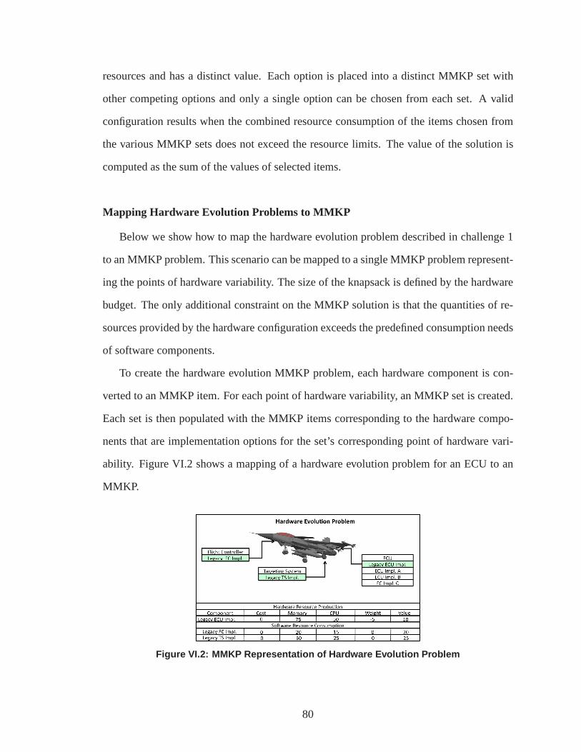
resources and has a distinct value. Each option is placed into a distinct MMKP set with

other competing options and only a single option can be chosen from each set. A valid

configuration results when the combined resource consumption of the items chosen from

the various MMKP sets does not exceed the resource limits. The value of the solution is

computed as the sum of the values of selected items.

Mapping Hardware Evolution Problems to MMKP

Below we show how to map the hardware evolution problem described in challenge 1

to an MMKP problem. This scenario can be mapped to a single MMKP problem represent-

ing the points of hardware variability. The size of the knapsack is defined by the hardware

budget. The only additional constraint on the MMKP solutionis that the quantities of re-

sources provided by the hardware configuration exceeds the predefined consumption needs

of software components.

To create the hardware evolution MMKP problem, each hardware component is con-

verted to an MMKP item. For each point of hardware variability, an MMKP set is created.

Each set is then populated with the MMKP items correspondingto the hardware compo-

nents that are implementation options for the set’s corresponding point of hardware vari-

ability. Figure VI.2 shows a mapping of a hardware evolutionproblem for an ECU to an

MMKP.

Figure VI.2: MMKP Representation of Hardware Evolution Pro blem

80

In Figure VI.2 the software does not have any points of variability that are eligible

for evolution. Since there is no variability in the software, the exact amount of each re-

source consumed by the software is known. The M-HEU approximation algorithm (or an

exhaustive search algorithm, such as a linear constraint solver) uses this hardware evolu-

tion MMKP problem, the predefined resource consumption, andthe predefined external

resource (budget) requirements to determine which ECUs to purchase and install. The so-

lution to the MMKP is the hardware components that should be chosen to implement each

point of hardware variability.

Mapping Software Evolution Problems to MMKP

We now show how to map the software evolution problem described in challenge 2to

an MMKP problem. In this case, the hardware configuration cannot be altered, as shown

in Figure VI.3. The hardware thus produces a predetermined amount of each resource.

Figure VI.3: MMKP Representation of Software Evolution Pro blem

Similar to the previous section. the fiscal budget availablefor software purchases is also

predetermined. Only the software evolution MMKP problem must therefore be solved to

determine an optimal solution.

As shown in thesoftware problemportion of Figure VI.3, each point of software vari-

ability becomes a set that contains the corresponding controller implementations. For each

81

set there are multiple implementations that can serve as thecontroller. This software evolu-

tion problem—along with the software budget and the resources available for consumption

as defined by the hardware configuration—can be used by an MMKPalgorithm to deter-

mine a valid selection of throttle and brake controllers.

Hardware/Software Co-Design with ASCENT

Several approximation algorithms can be applied to solve single MMKP problems, as

described in the previous two sections. These algorithms, however, cannot solve cases in

which there are points of variability in both hardware and software that have eligible evo-

lution options. In this situation, the variability in the production of resources from hard-

ware and the consumption of resources by software requires solving two MMKP problems

simultaneously, rather than one. In prior work we developedtheAllocation-baSed Config-

uration Exploration Technique(ASCENT) to determine valid, low-cost solutions for these

types of dual MMKP problems [122].

ASCENT is a search-based, hardware/software co-design approximation algorithm that

maximizes the software value of systems while ensuring thatthe resources produced by the

hardware MMKP solution are sufficient to support the software MMKP solution [122]. The

algorithm can be applied to system design problems in which there are multiple producer/-

consumer resource constraints. In addition, ASCENT can enforce external resource con-

straints, such as adherence to a predefined budget.

The software and hardware evolution problem described in challenge 4 must be mapped

to two MMKP problems so ASCENT can solve them. The hardware and software evolu-

tion MMKP problems are prepared as shown in Figure VI.4. Thisevolution differs from

the problems described in the section entitled “Mapping Hardware Evolution Problems to

MMKP”, since all software implementations are now eligiblefor evolution, thereby dra-

matically increasing the amount of variability. These two problems—along with the total

budget—are passed to ASCENT, which then searches the configuration space at various

82

Figure VI.4: MMKP Representation of Unlimited Evolution Pr oblem

budget allocations to determine a configuration that optimizes a linear function computed

over the software MMKP solution. Since ASCENT utilizes an approximation algorithm,

the total time to determine a valid solution is usually small. In addition, the solutions it

produces average over 90% of optimal [122].

Formal Validation of Evolved DRE Systems

There are many complex constraints that make it hard to determine the validity of a

DRE system configuration. These constraints include the resource production/consumption

relationship of tightly coupled hardware/software, the presence of multiple external re-

source constraints (such as component cost and power consumption) consumed by hard-

ware and/or software components, and functional constraints that restrict which compo-

nents are required/disallowed for implementation due to other component selections.

This section presents a formal model that can be used to determine the validity of a sys-

tem based on the selection of hardware and software components. The model takes into ac-

count the presence of external resources, such as total project budget, power consumption,

and heat production, the complex hardware/software resource production/consumption re-

lationship, and functional constraints between multiple components. The empirical results

section uses thismodel to define experiment parameters and determine the validity of gen-

erated final system configurations.

83

Top-Level Definition of an Evolved DRE System

A goal of evolving DRE systems is often to produce a new systemconfiguration that

meets all system-wide constraints and increases system value. The final system configura-

tion produced by software evolution analysis can be described as a 4-tuple:

F =< H,S,B,V >

where

• H is a set of variables describing the hardware portion of the final system configura-

tion, including the set of hardware components selected, their external resource consump-

tion and computational resource production.

• Sdefines the software portion of the systems consisting of thea set of software com-

ponents, their total cost, and the total value added to the system.

• B represents the total project budget of evolving a system. The project budget is

the total funding available for purchasing hardware and software components. If the total

project budget is exceeded, then system designers will not be able to purchase required

components resulting in an incomplete final system configuration.

• V is the total value of the hardware and software components comprising the final

system configuration.

Definition of Hardware Partition

The hardware partition of system provides the computational resources, such as mem-

ory and processing power, to support the software components of the system. To provide

these resources, the hardware of the system must also consume physical resources, such as

weight, power, and heat. Unlike software components, however, some hardware compo-

nents can increase the availability of these resources. Thehardware partition of a system is

represented by the following 5-tuple:

84

H =< HC,α(HC),ρ(HC),Ex,V(HC)>

where

• HC is the set of hardware components that make up the hardware ofthe system. These

components support one or more software components or add additional resources, such as

power, to support other hardware components.

• α(HC) is a tuple containing the total resource consumption valuesof the set of hard-

ware componentsHC.

• ρ(HC) defines the total hardware resources, such as power and heat dissipation, pro-

duced by the set of hardware componentsHC.

•Exspecifies the predetermined hardware resource limitations, such as available weight

capacity and power, provided by the system environment. In some cases purchasing hard-

ware components can increase these values, as defined byρ(HC). For example, purchasing

a battery can increase the power availability of the system,but may increase system cost,

weight, and heat generation.

•V(HC) is the total value added to the system by the set of hardware componentsHC.

External Resource Limitations

The hardware partition of a system must meet several external resource constraints that

are predetermined based on the application of the system. For example, avionics systems,

such as unmanned aerial vehicles, do not remain perpetuallyconnected to an external power

source. Instead, on-board batteries provide a finite power source. The following 4-tuple

represents the external resources available for consumption by the hardwareH:

Ex=< BH ,PH ,HHWH >

where

85

• BH is the hardware budget, which is the maximum amount of money available to pur-

chase Hardware components. OnceBH is exhausted, no additional hardware components

can be added to the system. No hardware components can be purchased to augmentBH .

• PH is the total amount of external power available to the system. For systems in

which power is unlimited, this value can be set to∞. Some evolution scenarios may allow

the purchase of batteries or other hardware to increase the available power pastPH , though

this is usually at the expense ofBH , WH , and/orHH .

• HH defines the maximum amount of heat that can be generated by thehardwareH

of the system. In certain applications, such as automated manufacturing systems, exceed-

ing predefined temperature limits can cause hardware to failor corrupt the product being

manufactured. Additional hardware components, such as heat sinks, can be purchased to

counteract heat produced by hardware and thereby increase the heat capacity of they sys-

tem.

•WH represents the weight limit of the final system configurationas a result ofH. Each

additional hardware component increases the weight of the system by a distinct amount.

Many DRE systems have strict requirements on the total weight of the system. For example,

each pound of hardware added to avionics systems requires roughly 4 additional supporting

pounds of infrastructure and fuel. No hardware components are capable of reducing the

weight capacity of a system.

Hardware Components

The hardware component selectionHC of the hardware partition determines the com-

putational resources, such as memory and processor utilization, that are available to sup-

port the software partition of the system. Hardware components can also produce other

resources (such as power and heat dissipation) to validate the selection of additional hard-

ware and increase elements ofEx beyond their initial capacities. The set of N chosen

hardware components is by the following N-tuple:

86

HC=< Hc0,Hc1.....Hcn >

where

• Hci is a hardware component included in the final configuration. Each hardware

component consumes multiple external resources. The totalresource consumption of a

hardware componentHc is defined by the following 4-tuple:

Rc(Hc) =<Cost(Hc),Pow(Hc),W(Hc),He(Hc),>

where

• Cost(Hc) is the cost of purchasing hardware componentHc.

• Pow(Hc) is the power consumed byHc.

• W(Hc) is the weight added to the final configuration by includingHc.

• He(Hc) is the heat generated byHc.

Hardware components will either support one or more software components or add

additional hardware resources, such as power to the system.The following equation defines

the set of software components that are deployed to hardwarecomponentHc:

Dep(Hc) =< Sc0,Sc1.....Scn >

Hardware components (such as heat sinks and batteries) provide additional resources

(such as heat capacity and power) to the system. These components, however, do not

produce any computational resources and may consume other external resources (such as

project budget and weight). The total resource production of hardware componentHc is

defined by the following tuple:

Rp(Hc) =< r0, r1, r2, ...rn >

87

wherer i is a resource produced by componentHc.

Hardware components must also consume several resources (such as project budget

and weight capacity) to function. The resource consumptionof hardware componentHc is

defined as:

Rc(Hc) =< r0, r1, r2....rn >

wherer i represents a distinct hardware resource (such as power or cost). The total

resource consumption of all hardware componentsHC is defined by the following 4-Tuple:

α(HC) =< β (HC),δ (HC),τ(HC),m(HC)>

where

• β is the total cost of all hardware componentsHC.

• δ is the total power consumption of all hardware componentsHC.

• τ is the total weight of all hardware componentsHC.

• m is the total heat consumption of hardware componentsHC.

The total resource consumption of each type of resource inα is determined by the sum-

mation of each type of resourcer i across all hardware componentsHC. If we assume that

r0 is the cost of a hardware component,r1 represents the power consumption,r2 the weight

of the component, andr3 the heat generation of the component, the resource consumption

totals is given by the following equations:

β (HC) =|HC|

∑i=0

Rc(HCi)0

δ (HC) =|HC|

∑i=0

Rc(HCi)1

τ(HC) =|HC|

∑i=0

Rc(HCi)2

88

m(HC) =|HC|

∑i=0

Rc(HCi)3

Finally, each hardware component adds a discrete amount of value to the system. The

amount of value added to the system by hardware componentsHC is defined by the fol-

lowing equation:

V(HC) =|HC|

∑i=0

v(HCi)

wherev(HCi) gives the value of including hardware componentHCi in the final system

configuration.

Definition of Software Partition

The software partition consists of software components that provide functionality and

add value to the system. The software partition is comprisedof a set of software compo-

nents that consume the computational resources of the hardware components to which they

are deployed. Each software component consumes multiple resources, carries a purchase

cost, and adds a discrete amount of value to the system. The software partitionSof a final

configuration is defined by the follow 3-tuple:

S=< θ(SC),V(SC),SC>

where

• θ(SC) is the total cost of the software componentsSCof the final configuration.

• V(SC) is the total value of the software componentsSCcomprising the final system

configurations.

• SCis the set of software components that make up the final systemconfiguration.

The set of software componentsSCconsists of one or more individual software compo-

nents, each costing different amounts of money to purchase and adding distinct amounts of

89

value to the system. The total cost of the software componentsSCis determined by taking

the sum of the values of all software components in the system:

θ(SC) =|SC|

∑i=0

Rc(SCi)0

The value added by all components,V(SC), is calculated with the following equation:

V(SC) =|SC|

∑i=0

v(SCi)

Each software component also consumes one or more computational resources. These

resources (such as memory and processing power) are provided by the hardware component

to which the software component(s) are deployed. A softwarecomponent that consumesn

resources is defined by the following n-tuple:

Rc(Sc) =< r0, r1, r2, ...rn >

wherer i is the amount of the resource consumed.

Determining if a Final System Configuration is Valid

The hardwareH and softwareS for are selected for a final system configurationF

must satisfy several constraints to be considered valid. The first constraint is that external

resources, such as weight and power, must not be over consumed by the hardware. Second,

the purchase price of all components must not exceed the total project budget. Finally, no

set of software components can consume more resources than provided by the hardware

component to which they are deployed.

External Resource Consumption Does Not Exceed Production

The following equation determines if the total external resource consumption exceeds

external resource availability:

90

σ(HC) =(

|HC|

∑i=0

Rp(HCi)+Ex)

−|HC|

∑i=0

Rp(HCi)

This equation adds the total hardware resource production to the predefined external

resource limits to give the total external resource availability. The total resource consump-

tion of the hardware componentsHC is then subtracted from the total external resource

availability. If no elements inσ are negative the external resources are not over consumed

by the hardware. This constraint is violated, however, if the following equation yields a

negative value:

ExCon(F) = min(0,σ(HC))

If ExCon is less than zero the available external resources are not sufficient to support

the external resource consumption of the hardware.

Project Budget Exceeds Component Costs

Each final system configurationF has a project budgetB defining the maximum amount

of money that can be spent purchasing hardware and software components. If this amount

is exceeded, however, sufficient funds will not be availableto purchase allHC andSCof

H andS, thereby invalidating the final configurationF. The total cost of the system can be

calculated with the following equation:

TotCost(HC,SC)= β (HC)+θ(SC)

CostCon(F) = min(0,B−TotCost(HC,SC))

If the value ofCostCon(F) is less than zero, then insufficient funds are available to

purchase componentsHC andSC.

91

Hardware Resource Production Exceeds Software Resource Consumption

In a final configurationF, the software componentsSCare deployed to the hardware

componentsHC. Each software componentScconsumes computational resourcesr i (such

as memory and processing power) provided by the hardware componentHc to which it is

deployed. The sum of the consumption of each resource of all software components allo-

cated to a hardware component must not exceed the resource production of each resource

produced. The following equation,λ (HC) determines the resource consumption of the

software components deployed to hardware componentsHC:

λ (HC) = ∀HC,∀r ∈ Rp(HCi), r i − (|Dep(HCi)|

∑j=0

Rc(Dep(Hc) j))

HSRCon(F) = min(0,λ (HC))

The final hardware/software resource constraint,HSRFCon(F), determines if the re-

source production of any hardware component inHC is over consumed by the software it

supports. IfHSRFCon(F) is less than 0 the constraint is violated and the final configuration

F is invalid.

Validating a Final System Configuration

The following three constraints must be satisfied to ensure the validity of a final system

configurationF:

• Resource availability must exceed consumption as determined byExCon(F),

• Component costs must be less than the project budget as given byCostCon(F), and

• The resource production of the hardware componentsHC must exceed the resource

consumption of the software componentsSCas given byHRSCon f(F).

The validity of the final system configurationF is conveyed by the following equation:

92

Validity(F) = ExCon(F)+CostCon(F)+HSRCon f(F)

A final system configurationF is considered valid ifValidity(F) is equal to zero.

Empirical Results

This section determines valid, high-value, evolution configurations for the scenarios de-

scribed in the section entitled “Challenges of DRE System Evolution Decision Analysis”

using empirical data obtained from three different algorithmic techniques: (1) exhaustive

search techniques, (2) the M-HEU algorithm for solving single MMKP problem instances,

and (3) the ASCENT technique for solving unlimited evolution problems, all of which are

described in the previous solution sections. These resultsdemonstrate that each algorithm

is effective for certain types of MMKP problems. Moreover, anear-optimal solution can be

found if the correct technique is used. Each set represents apoint of design variability and

problems with more sets have more variability. Moreover, the ASCENT and M-HEU algo-

rithms can be used to determine solutions for large-scale problems that cannot be solved in

a feasible amount of time with exhaustive search algorithms.

Experimentation Testbed

All algorithms were implemented in Java and all experimentswere conducted on an

Apple MacbookPro with a 2.4 GHz Intel Core 2 Duo processor, 2 gigabytes of RAM,

running OS X version 10.5.5, and a 1.6 Java Virtual Machine (JVM) run in client mode.

For our exhaustive MMKP solving technique—which we call thelinear constraint solver

(LCS)—we used a branch and bound solver built on top of the Java Choco Constraint

Solver (choco.sourceforge.net). The M-HEU heuristic solver was a custom im-

plementation that we developed with Java. The ASCENT algorithm was also based on a

custom implementation with Java.

93

Simulation MMKP problems were randomly generated. In this process, the number

of sets, the minimum and maximum number of items per set, the minimum and maximum

resource consumption/production per item, and the minimumand maximum value per item,

are the inputs to the MMKP problem generator. The generator produces an MMKP problem

consisting of the specified number of sets. The number of items in each set, the resource

consumption/production of each item, and the value of each item, are randomly selected

within the specified bound for each parameter. This generation process is described further

in [122].

Hardware Evolution with Predefined Resource Consumption

Figure VI.5: Hardware Evolution Solve Time vs Number of Sets

This experiment investigates the use of a linear constraintsolver and the use of the

M-HEU algorithm to solve the challenge described in challenge 1, where the software

components are fixed. This type of system based on the formal definition of a system

configurationF.In this type of evolution problem, theS of the F tuple is fixed. For ease

of explanation, we also assumed that with the exception of budgetB, all values ofEx are

abundantly available.

We first tested for the total time needed for each algorithm torun to completion. We

then examined the optimality of the solutions generated by each algorithm. We ran these

tests for several problems with increasing set counts, thereby showing how each algorithm

performed with increased design variability.

94

Figure VI.5 shows the time required to generate a hardware configuration if the soft-

ware configuration is predefined.1 Since only a single MMKP problem must be solved,

we use the M-HEU algorithm. As set size increases, the time required for the linear con-

straint solver increases rapidly. If the problem consists of more sets, the time required for

the linear constraint solver becomes prohibitive. The M-HEU approximation algorithm,

however, scaled much better, finding a solution for a problemwith 1,000 sets in∼15 sec-

onds. Figure VI.6 shows that both algorithms generated solutions with 100% optimality

Figure VI.6: Hardware Evolution Solution Optimality vs Num ber of Sets

for problems with 5 or less sets.

Regardless of the number of sets, the M-HEU algorithm completed faster than the linear

constraint solver without sacrificing optimality.

Figure VI.7: Software Evolution Solve Time vs Number of Sets

1Time is plotted on a logarithmic scale for all figures that show solve time.

95

Software Evolution with Predefined Resource Production

This experiment examines the use of a linear constraint solver and the M-HEU algo-

rithm to solve evolution scenarios in which the hardware components are fixed, as described

in challenge 2. In this type of problem, theH of the configurationF is predefined. We test

for the total time each algorithm needs to run to completion and examine the optimality of

solutions generated by each algorithm.

Figure VI.7 shows the time required to generate a software configuration generated if

the hardware configuration is predetermined. As with Challenge 2, the M-HEU algorithm

is used since only a single MMKP problem must be solved. Once again, LCS’s limited

scalability is demonstrated since the required solve time makes its use prohibitive for prob-

lems with more than five sets. The M-HEU solver scales considerably better and can solve

a problem with 1,000 sets in less than 16 seconds, which is fastest for all problems.

Figure VI.8 shows the optimality provided by each solver. Inthis case, the M-HEU

Figure VI.8: Software Evolution Solution Optimality vs Num ber of Sets

solver is only 80% optimal for problems with 4 sets. Fortunately, the optimality improves

with each increase in set count with a solution for a problem with 7 sets being 100% opti-

mal.

96

Unrestricted Software Evolution with Additional Hardware

This experiment examines the use of a linear constraint solver and the ASCENT algo-

rithm to solve the challenge described in challenge 4, in which no hardware or software

components are fixed. We first test for the total time needed for each algorithm to run to

completion and then examine the optimality of the solutionsgenerated by each algorithm.

Unrestricted evolution of software and hardware components has similar solve times to the

previous experiments.

Figure VI.9 shows that regardless of the set count for the MMKP problems, the AS-

CENT solver derived a solution much faster than LCS. This figure also shows that the

Figure VI.9: Unrestricted Evolution Solve Time vs Number of Sets

Figure VI.10: Unrestricted Evolution Solution Optimality vs Number of Sets

required solve time to determine a solution with LCS increases rapidly,e.g., problems that

have more than five sets require an extremely long solve time.The ASCENT algorithm

once again scales considerably better and can even solve problems with 1,000 or more sets.

97

Figure VI.11: LCS Solve Times vs Number of Sets

In this case, the optimality of the solutions found by ASCENTis low for problems with 5

sets, as shown in Figure VI.10.

Fortunately, the time required to solve with LCS is not prohibitive in these cases, so it

is still possible to find a solution with 100% optimality in a reasonable amount of time.

Comparison of Algorithmic Techniques

This experiment compared the performance of LCS to the performance of the M-HEU

and ASCENT algorithms for all challenges. As shown in FigureVI.11, the characteris-

tics of the problem(s) being solved have a significant impacton solving duration. Each

Figure VI.12: M-HEU & ASCENT Solve Times vs Number of Sets

challenge has more points of variability than the previous challenge. The solving time for

LCS thus increases as the number of the points of variabilityincreases. For all cases, the

LCS algorithm requires an exorbitant amount of time for problems with more than five

sets. In contrast, the M-HEU and ASCENT algorithms show no discernable correlation

98

Figure VI.13: Comparison of Solve Times for All Experiments

between the amount of variability and the solve time. In somecases, problems with more

sets require more time to solve than problems with less sets,as shown in Figure VI.12.

Figure VI.14: Comparison of Optimalities for All Experimen ts

Figure VI.13 compares the scalability of the three algorithms.

Figure VI.15: Taxonomy of Techniques

This figure shows that LCS requires the most solving time in all cases. Likewise, the

ASCENT and M-HEU algorithms scale at approximately the samerate for all problems and

are far superior to the LCS algorithm. The optimality of the ASCENT and M-HEU algo-

rithms is near-optimal only for problems with five or more sets, as shown in Figure VI.14.

The exception to this trend occurs if there are few points of variability,e.g., when there

99

are few sets and the software is predetermined. These findings motivate the taxonomy

shown in Figure VI.15 that describes which algorithm is mostappropriate, based on prob-

lem size and variability.

100

CHAPTER VII

MODEL-DRIVEN AUTO-SCALING OF GREEN CLOUD COMPUTINGINFRASTRUCTURE

Challenge Overview

This chapter presents an application of automated model-driven configuration to cloud

computing paradigms. We demonstrate how the auto-scaling policies of cloud comput-

ing environments can be augmented with automated configuration techniques to meet the

dynamic configuration requirements of application demand.Further, we show that these

techniques can be used to generate configurations with substantially reduced operating cost

and emissions while ensuring that Service Level Agreements(SLAs) are upheld.

Introduction

Current trends and challenges.By 2011, power consumption of computing data cen-

ters is expected to exceed 100,000,000,00 kilowatt-hours(kWh) and generate over 40,568,000

tons of CO2 emissions [1, 23, 93]. Since data centers operate at only 20-30% utilization,

70-80% of this power consumption is lost due to over-provisioned idle resources, resulting

in roughly 29,000,000 tons of unnecessary CO2 emissions [1, 23, 93]. Applying new com-

puting paradigms, such as cloud computing with auto-scaling, to increase server utilization

and decrease idle time is therefore paramount to creating greener computing environments

with reduced power consumption and emissions [8,11,15,21,75].

Cloud computing is a computing paradigm that uses virtualized server infrastructure

and auto-scaling to provision virtual OS instances dynamically [86]. Rather than over-

provisioning an application’s infrastructure to meet peakload demands, an application can

auto-scaleby dynamically acquiring and releasing virtual machine (VM) instances as load

fluctuates. Auto-scaling increases server utilization anddecreases idle time compared with

101

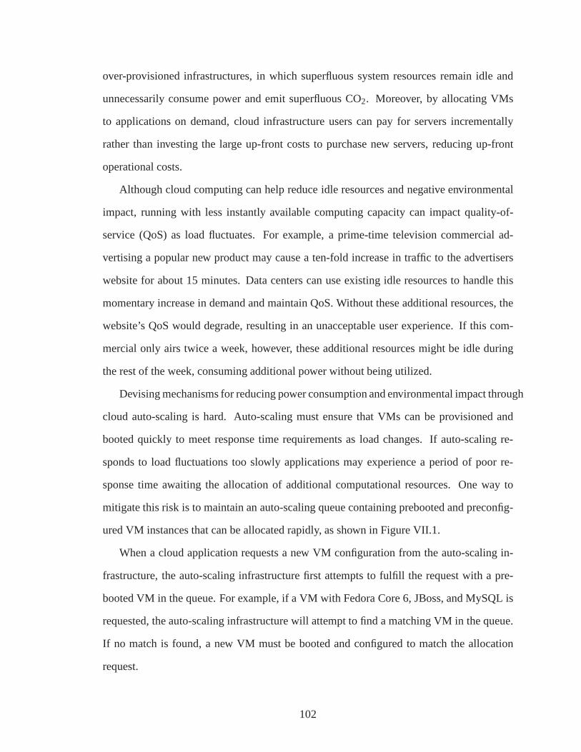
over-provisioned infrastructures, in which superfluous system resources remain idle and

unnecessarily consume power and emit superfluous CO2. Moreover, by allocating VMs

to applications on demand, cloud infrastructure users can pay for servers incrementally

rather than investing the large up-front costs to purchase new servers, reducing up-front

operational costs.

Although cloud computing can help reduce idle resources andnegative environmental

impact, running with less instantly available computing capacity can impact quality-of-

service (QoS) as load fluctuates. For example, a prime-time television commercial ad-

vertising a popular new product may cause a ten-fold increase in traffic to the advertisers

website for about 15 minutes. Data centers can use existing idle resources to handle this

momentary increase in demand and maintain QoS. Without these additional resources, the

website’s QoS would degrade, resulting in an unacceptable user experience. If this com-

mercial only airs twice a week, however, these additional resources might be idle during

the rest of the week, consuming additional power without being utilized.

Devising mechanisms for reducing power consumption and environmental impact through

cloud auto-scaling is hard. Auto-scaling must ensure that VMs can be provisioned and

booted quickly to meet response time requirements as load changes. If auto-scaling re-

sponds to load fluctuations too slowly applications may experience a period of poor re-

sponse time awaiting the allocation of additional computational resources. One way to

mitigate this risk is to maintain an auto-scaling queue containing prebooted and preconfig-

ured VM instances that can be allocated rapidly, as shown in Figure VII.1.

When a cloud application requests a new VM configuration fromthe auto-scaling in-

frastructure, the auto-scaling infrastructure first attempts to fulfill the request with a pre-

booted VM in the queue. For example, if a VM with Fedora Core 6,JBoss, and MySQL is

requested, the auto-scaling infrastructure will attempt to find a matching VM in the queue.

If no match is found, a new VM must be booted and configured to match the allocation

request.

102

Figure VII.1: Auto-scaling in a Cloud Infrastructure

Open problem→ determining green settings, such as the size and properties of the

auto-scaling queue shared by multiple applications with different VM configurations [19].

The chosen configurations must meet the configuration requirements of multiple applica-

tions and reduce power consumption without adversely impacting QoS. For example, a

web application may request VM instances configured as database, middle-tier Enterprise

Java Beans (EJB), or front-end web servers. Determining howto capture and reason about

the configurations that comprise the auto-scaling queue is hard due to the large number of

configuration options (such as MySQL and SQL Server databases, Ubuntu Linux and Win-

dows operating systems, and Apache HTTP and IIS/Asp.Net webhosts) offered by cloud

infrastructure providers.

It is even harder to determine the optimal queue size and types of VM configurations

that will ensure VM allocation requests can be serviced quickly enough to meet a required

auto-scaling response time limit. Cost optimization is challenging because each configu-

ration placed into the queue can have varying costs based on the hardware resources and

software licenses it uses. Energy consumption minimization is also hard since hardware

resources can consume different amounts of power.

Solution approach→ Auto-scaling queue configuration derivation based on fea-

ture models. This chapter presents a model-driven engineering (MDE) approach called

103

theSmart Cloud Optimization for Resource Configuration Handling(SCORCH). SCORCH

captures VM configuration options for a set of cloud applications and derives an optimal

set of virtual machine configurations for an auto-scaling queue to provide three green com-

puting contributions:

• An MDE technique for transforming feature model representations of cloud VM con-

figuration options into constraint satisfaction problems (CSPs) [53,62], where a set of vari-

ables and a set of constraints govern the allowed values of the variables.

• An MDE technique for analyzing application configuration requirements, VM power

consumption, and operating costs to determine what VM instance configurations an auto-

scaling queue should contain to meet an auto-scaling response time guarantee while mini-

mizing power consumption.

• Empirical results from a case study using Amazon’s EC2 cloudcomputing infrastruc-

ture (aws.amazon.com/ec2) that shows how SCORCH minimizes power consumption

and operating cost while ensuring that auto-scaling response time requirements are met.

Challenges of Configuring Virtual Machines in Cloud Environments

Reducing unnecessary idle system resources by applying auto-scaling queues can po-

tentially reduce power consumption and resultingCO2 emissions significantly. QoS de-

mands, diverse configuration requirements, and other challenges, however, make it hard to

achieve a greener computing environment. This section describes three key challenges of

capturing VM configuration options and using this configuration information to optimize

the setup of an auto-scaling queue to minimize power consumption.

Challenge 1: Capturing VM Configuration Options and Constraints

Cloud computing can yield greener computing by reducing power consumption. A

cloud application can request VMs with a wide range of configuration options, such as

type of processor,

104

OS, and installed middleware, all of which consume different amounts of power. For

example, the Amazon EC2 cloud infrastructure supports 5 different types of processors, 6

different memory configuration options, and over 9 different OS types, as well as multiple

versions of each OS type [47]. The power consumption of theseconfigurations range from

150 to 610 watts per hour.

The EC2 configuration options cannot be selected arbitrarily and must adhere to myriad

configuration rules. For example, a VM running on Fedora Core6 OS cannot run MS

SQL Server. Tracking these numerous configuration options and constraints is hard. The

sections entitled “SCORCH Cloud Configuration Models” and “SCORCH Configuration

Demand Models” describe how SCORCH uses feature models to alleviate the complexity

of capturing and reasoning about configuration rules for VM instances.

Challenge 2: Selecting VM Configurations to Guarantee Auto-scaling Speed Require-

ments

While reducing idle resources results in less power consumption and greener computing

environments, cloud computing applications must also meetstringent QoS demands. A

key determinant of auto-scaling performance is the types ofVM configurations that are

kept ready to run. If an application requests a VM configuration and an exact match is

available in the auto-scaling queue, the request can be fulfilled nearly instantaneously. If

the queue does not have an exact match, it may have a running VMconfiguration that can

be modified to meet the requested configuration faster than provisioning and booting a VM

from scratch. For example, a configuration may reside in the queue that has the correct

OS but needs to unzip a custom software package, such as a pre-configured Java Tomcat

Web Application Server, from a shared file system onto the VM.Auto-scaling requests can

thus be fulfilled with both exact configuration matches and subset configurations that can

be modified faster than provisioning a VM from scratch.

Determining what types of configurations to keep in the auto-scaling queue to ensure

105

that VM allocation requests are serviced fast enough to meeta hard allocation time con-

straint is hard. For one set of applications, the best strategy may be to fill the queue with

a common generic configuration that can be adapted quickly tosatisfy requests from each

application. For another set of applications, it may be faster to fill the queue with the virtual

machine configurations that take the longest to provision from scratch. Numerous strate-

gies and combinations of strategies are possible, making ithard to select configurations to

fill the queue that will meet auto-scaling response time requirements. The section entitled

“Runtime Model Transformation to CSP and Optimization” shows how SCORCH captures

cloud configuration options and requirements as cloud configuration feature models, trans-

forms these models into a CSP, and creates constraints to ensure that a maximum response

time limit on auto-scaling is met.

Challenge 3: Optimizing Queue Size and Configurations to Minimize Energy Con-

sumption and Operating Cost

A further challenge for developers is determining how to configure the auto-scaling

queue to minimize the energy consumption and costs requiredto maintain it. The larger the

queue, the greater the energy consumption and operating cost. Moreover, each individual

configuration within the queue varies in energy consumptionand cost. For example, a

“small” Amazon EC2 VM instance running a Linux-based OS consumes 150W and costs

$0.085 per hour while a "Quadruple Extra Large" VM instance with Windows consumes

630W and costs $2.88 per hour.

It is hard for developers to manually navigate tradeoffs between energy consumption,

operating costs, and auto-scaling response time of different queue sizes and sets of VM

configurations. Moreover, there are an exponential number of possible queue sizes and

configuration options that complicates deriving the minimal power consumption/operating

cost queue configuration that will meet auto-scaling speed requirements. The section enti-

tled “Runtime Model Transformation to CSP and Optimization” describes how SCORCH

106

uses CSP objective functions and constraints to derive a queue configuration that minimizes

power consumption and operating cost.

The Structure and Functionality of SCORCH

This section describes how SCORCH resolves the challenges in the previous section

by using (1) models to capture virtual machine configurationoptions explicitly, (2) model

transformations to convert these models into CSPs, (3) constraint solvers to derive the

optimal queue size, and (4) contained VM configuration options to minimize energy con-

sumption and operating cost while meeting auto-scaling response time requirements.

Figure VII.2: SCORCH Model-Driven Process

The SCORCH MDE process is shown in Figure VII.2 and describedbelow:

1. Developers use a SCORCHcloud configuration modelto construct a catalog of

configuration options that are available to VM instances.

2. Each application considered in the auto-scaling queue configuration optimization

provides aconfiguration demand modelthat specifies the configuration for each type of

virtual machine instance the application will request during its execution lifecycle.

3. Developers provide aconfiguration adaptation time modelthat specifies the time

required to add/remove a feature from a configuration.

4. Developers provide anenergy modelthat specifies the power consumption required

107

to run a VM configuration with each feature present in the SCORCH cloud configuration

model.

5. Developers provide acost modelthat specifies the cost to run a VM configuration

with each feature present in the SCORCH cloud configuration model.

6. The cloud configuration model, configuration demand models,and load estimation

model are transformed into a CSP and a constraint solver is used to derive the optimal

auto-scaling queue setup.

The remainder of this section describes the structure and functionality of each model

defined and used by SCORCH.

SCORCH Cloud Configuration Models

A key consideration in SCORCH is modeling the catalog of VM configuration options.

Amazon EC2 offers many different options, such as Linux vs. Windows operating systems,

SQL Server vs. MySQL databases, and Apache HTTP vs. IIS/Asp.Net webhosts. This

model provides developers with a blueprint for constructing a request for a VM instance

configuration and checking its correctness. The queue configuration optimization process

also uses this model to ensure that valid configurations are chosen to fill the queue.

To manage the complexity of representing VM instance configuration options, SCORCH

usesfeature models[53], which describe commonality and variability in a configurable

software platform via an abstraction called afeature. Features can describe both high-level

functional variations in the software,e.g., whether or not the underlying software can load

balance HTTP requests. A feature can also represent implementation-specific details,e.g.,

whether or not Ubuntu 9.10 or Fedora is used.

Feature models use a tree structure to define the relationships between the various fea-

tures and encode configuration rules into the model,e.g., a VM configuration can include

only a single operating system, such as Ubuntu 9.10 or Fedora. Some features may require

108

other features to be present to function,e.g., the JBOSS v6 feature cannot be chosen

without also selecting theJBOSS feature.

A configuration of the software platform is defined by a selection of features from

the feature model. The most basic rule of configuration correctness is that every selected

feature must also have its parent feature selected. This rule also implies that every correct

feature selection must include the root feature. Moreover,the feature selection must adhere

to the constraints on the parent-child relationships encoded into the feature model.

Developers use the SCORCH cloud configuration model to express the available con-

figuration options for VM instances as a feature model. The configuration adaption time

model’s information is captured as attributes of the features in the SCORCH cloud configu-

ration model. Each feature can be annotated with an integer attribute that specifies the time

in milliseconds to add/remove the given feature from a configuration.

The energy model and cost model are also captured using attributes in the SCORCH

cloud configuration model. Each feature impacting the energy consumption or operating

cost of a configuration is annotated with an energy attributethat specifies the energy con-

sumption per hour and cost attribute that specifies the operating cost per hour to have a

booted VM configuration in the queue with that feature. For example, these attributes can

be used to model the cost of the “Small” vs. “Quadruple Extra Large” computing node size

features of an Amazon EC2 VM configuration.

SCORCH Configuration Demand Models

Applications are auto-scaled at runtime by dynamically requesting and releasing VM

instances. When a new VM instance is requested, the desired configuration for the instance

is provided. SCORCH requires each application to provide a model of the VM instance

configurations that it will request over its lifetime.

Developers construct SCORCH configuration demand models todictate what VM con-

figurations an application will request. The configuration demand models use a textual

109

domain-specific language to describe each configuration requested as a selection of fea-

tures from the SCORCH cloud configuration model.

Runtime Model Transformation to CSP and Optimization

Using feature models to capture VM configuration options allows the use of constraint

solvers to select a group of features to optimize an objective function. In the context of

SCORCH, the cloud configuration model and configuration demand models are converted

into a CSP where a solution is a valid set of configurations forthe VM instances in the auto-

scaling queue. The objective function of the CSP attempts toderive a mix of configurations

that minimizes the energy consumption and cost of maintaining the queue while ensuring

that any hard constraints on the time to fulfill auto-scalingrequests are met.

The conversion of feature selection problems into CSPs has been described in prior

work [14,119]. Feature configuration problems are converted into CSPs where the selection

state of each feature is represented as a variable with domain {0,1}. The constraints are

designed so that a valid labeling of these variables yields avalid feature selection from the

feature model.

A CSP for a feature selection problem can be described as a 3-tuple:

P=< F,C,γ >

where:

• F is a set of variables describing the selection state of each feature. For each feature,

fi ∈ F, if the feature is selected in the derived configuration, then fi = 1. If the ith feature

is not selected, thenfi = 0.

• C captures the rules from the feature model as constraints on the variables inF . For

example, if theith feature requires thejth feature,C would include a constraint:( fi = 1)⇒

( f j = 1).

110

• γ is an optional objective function that should be maximized or minimized by the

derived configuration.

Building a CSP to derive a set of configurations for an auto-scaling queue uses a similar

methodology. Rather than deriving a single valid configuration, however, SCORCH tries to

simultaneously derive both the size of the auto-scaling queue and a configuration for each

position in the auto-scaling queue. If SCORCH derives a sizefor the queue ofK, therefore,

K different feature configurations will be derived for theK VM instances that need to fill

the queue.

The CSP for a SCORCH queue configuration optimization process can be described

formally as the 8-tuple

P=< S,Q,C,D,E,L,T,M,γ >

, where:

• S is the auto-scaling queue size, which represents the numberof prebooted VM in-

stances available in the queue. This variable is derived automatically by SCORCH.

• Q is a set of sets that describes the selection state of each VM instance configuration

in the queue. The size ofQ is Z if there areZ distinct types of configurations specified in

the configuration demand models. Each set of variables,Qi ∈ Q, describes the selection

state of features for one VM instance in the queue. For each variable,qi j ∈ Qi , if qi j = 1 in

a derived configuration, it indicates that thejth feature is selected by theith VM instance

configuration.

• C captures the rules from the feature model as constraints on the variables in all

setsQi ∈ Q. For example, if the kth feature requires thejth feature,C would include a

constraint:∀Qi ∈ Q, (qik = 1)⇒ (qi j = 1).

• D contains the set of configuration demand models contributedby the applications.

Each demand modelDi ∈ D represents a complete set of selection states for the features

in the feature model. If thejth feature is requested by theith demand model, thendi j ∈

111

Di ,di j = 1. The demand models can be augmented with expected load per configuration,

which is a focus of future work.

• E is the cost model that specifies the energy consumption resulting from including

the feature in a running VM instance configuration in the auto-scaling queue. For each

configurationDi ∈ D a variableEi ∈ E specifies the energy consumption of that feature.

These values are derived from annotations in the SCORCH cloud configuration model.

• L is the cost model that specifies the cost to include the feature in a running VM

instance configuration in the auto-scaling queue. For each configurationDi ∈ D a variable

Li ∈ L specifies the cost of that feature. These values are derived from annotations in the

SCORCH cloud configuration model.

• T is the configuration time model that defines how much time is needed to add/-

remove a feature from a configuration. The configuration timemodel is expressed as a set of

positive decimal coefficients, whereti ∈ T is the time required to add/remove theith feature

from a configuration. These values are derived from the annotations in the SCORCH cloud

configuration model.

• γ is the cost minimization objective function that is described in terms of the variables

in D, Q, andL.

• M is the maximum allowable response time to fulfill a request toallocate a VM with

any requested configuration from the demand models to an application.

Response Time Constraints and CSP Objective Function

SCORCH defines an objective function to attempt to minimize the cost of maintaining

the auto-scaling queue, given a CSP to derive configurationsto fill the queue. Moreover,

we can define constraints to ensure that a maximum response time bound is adhered to by

the chosen VM queue configuration mix and queue size that is derived.

112

We describe the expected response time,Rtx, to fulfill a requestDx from the configura-

tion demand model as:

Rtx = min(CT0 . . .CTn, boot(Dx)) (VII.1)

CTi =

∀qi j ∈ Qi , qi j = dx j0 (a),

∃qi j ∈ Qi , qi j ! = dx j ∑ t j(|qi j −dx j|) (b)

(VII.2)

where:

• Rtx is the expected response time to fulfill the request.

• n is the total number of features in the SCORCH cloud configuration model

• CTi is the expected time to fulfill the request if theith VM configuration in the queue

was used to fulfill it.

• boot(Dx) is the time to boot a new VM instance to satisfyDx and not use the queue

to fulfill it.

The expected response time,Rtx is equal to the fastest time available to fulfill the re-

quest, which will either be the time to use a VM instance in thequeueCTi or to boot a

completely new VM instance to fulfill the requestboot(Dx). The time to fulfill the request

is zero (or some known constant time) if a configuration exists in the queue that exactly

matches request (a). The time to fulfill the request with thatconfiguration is equal to the

time needed to modify the configuration to match the requested configurationDx if a given

VM configuration is not an exact match (b). For each featureqi j in the configuration that

does not match what is requested in the configuration,t j is the time incurred to add/remove

the feature. Across theZ distinct types of configuration requests specified in the configura-

tion demand models we can therefore limit the maximum allowable response time with the

constraint:

113

∀Dx ∈ D, M ≥ Rtx (VII.3)

With the maximum response time constraint in place, the SCORCH model-to-CSP

transformation process then defines the objective functionto minimize. For each VM in-

stance configuration,Qi , in the queue we define its energy consumption as:

Energy(Qi) =n

∑j=0

qi j E j

. The overall energy consumption minimization objective function, ε, is defined as the

minimization of the variableEnergy, where:

ε = Energy= Energy(Q0)+Energy(Q1)+ · · ·+Energy(Qk)

.

Similarly, the cost of each VM instance is defined as:

Cost(Qi) =n

∑j=0

qi j L j

. The overall cost minimization objective function,γ, is defined as the minimization of the

variableCost, where:

γ =Cost=Cost(Q0)+Cost(Q1)+ · · ·+Cost(Qk)

.

The final piece of the CSP is defining the constraints attachedto the queue size variable

S. We defineSas the number of virtual machine instance configurations that have at least

114

one feature selected:

Si =

∀qi j ∈ Qi , qi j = 00,

∃qi j ∈ Qi , qi j = 11

(VII.4)

S=Z

∑i=0

Si

Once the CSP is constructed, a standard constraint solver, such as the Java Choco con-

straint solver (choco.sourceforge.net), can be used to derive a solution. The fol-

lowing section presents empirical results from applying SCORCH with Java Choco to a

case study of an ecommerce application running on Amazon’s EC2 cloud computing in-

frastructure.

Empirical Results

This section presents a comparison of SCORCH with two other approaches for provi-

sioning VMs to ensure that load fluctuations can be met without degradation of QoS. We

compare the energy efficiency and cost effectiveness of eachapproach when provisioning

an infrastructure that supports a set of ecommerce applications. We selected ecommerce

applications due to the high fluctuations in workload that occur due to the varying seasonal

shopping habits of users. To compare the energy efficiency and cost effectiveness of these

approaches, we chose the pricing model and available VM instance types associated with

Amazon EC2.

We investigated three-tiered ecommerce applications consisting of web front end, mid-

dleware, and database layers. The applications required 10different distinct VM config-

urations. For example, one VM required JBOSS, MySql, and IIS/Asp.Net while another

required Tomcat, HSQL, and Apache HTTP. These applicationsalso utilize a variety of

computing instance types from EC2, such as high-memory, high-CPU, and standard in-

stances.

To model the traffic fluctuations of ecommerce sites accurately we extracted traffic

115

information from Alexa (www.alexa.com) for newegg.com (newegg.com), which is

an extremely popular online retailer. Traffic data for this retailer showed a spike of three

times the normal traffic during the November-December holiday season. During this period

of high load, the site required 54 VM instances. Using the pricing model provided by

Amazon EC2, each server requires 515W of power and costs $1.44 an hour to support the

heightened demand (aws.amazon.com/economics).

Experiment: VM Provisioning Techniques

Static provisioning. The first approach provisions a computing infrastructure equipped

to handle worst-case demand at all times. In this approach, all 54 servers run continuously

to maintain response time. This technique is similar to computing environments that permit

no auto-scaling. Since the infrastructure can always support the worst-case load, we refer

to this technique asstatic provisioning.

Non-optimized auto-scaling queue. The second approach augments the auto-scaling

capabilities of a cloud computing environment with an auto-scaling queue. In this ap-

proach, auto-scaling is used to adapt the number of resources to meet the current load that

the application is experiencing. Since additional resources can be allocated as demand in-

creases, we need not run all 54 servers continuously. Instead, an auto-scaling queue with

a VM instance for each of ten different application configurations must be allocated on

demand. We refer to this technique asnon-optimized auto-scaling queuesince the auto-

scaling queue is not optimized.

SCORCH. The third approach uses SCORCH to minimize the number of VM instances

needed in the auto-scaling queue, while ensuring that response time is met. By optimizing

the auto-scaling queue with SCORCH, the size of the queue canbe reduced by 80% to two

VM instances.

116

Power Consumption & Cost Comparison of Techniques

The maximum load for the 6 month period occurred in November and required 54 VM

instances to support the increased demand, decreasing to 26servers in December and finally

18 servers for the final four months. The monthly energy consumption and operational

costs of applying each response time minimization technique can be seen in Figure VII.3

and VII.4 respectively.

Figure VII.3: Monthly Power Consumption

Figure VII.4: Monthly Cost

Since the maximum demand of the ecommerce applications required 54 VM instances,

the static provisioning technique consumed the most power and was the most expensive,

with 54 VM instances prebooted and run continuously. The non-optimized auto-scaling

queue only required ten pre-booted VM instances and therefore reduced power consump-

tion and cost. Applying SCORCH yielded the most energy efficient and lowest cost infras-

tructure by requiring only two VM instances in the auto-scaling queue.

Figures VII.5 and VII.6 compares the total power consumption and operating cost of ap-

plying each of the VM provisioning techniques for a six monthperiod. The non-optimized

auto-scaling queue and SCORCH techniques reduced the powerrequirements and price

117

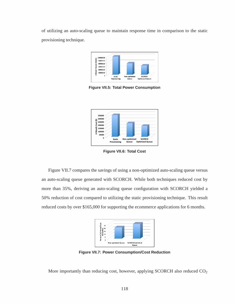
of utilizing an auto-scaling queue to maintain response time in comparison to the static

provisioning technique.

Figure VII.5: Total Power Consumption

Figure VII.6: Total Cost

Figure VII.7 compares the savings of using a non-optimized auto-scaling queue versus

an auto-scaling queue generated with SCORCH. While both techniques reduced cost by

more than 35%, deriving an auto-scaling queue configurationwith SCORCH yielded a

50% reduction of cost compared to utilizing the static provisioning technique. This result

reduced costs by over $165,000 for supporting the ecommerceapplications for 6 months.

Figure VII.7: Power Consumption/Cost Reduction

More importantly than reducing cost, however, applying SCORCH also reduced CO2

118

Figure VII.8: C02 Emissions

emissions by 50%, as shown in Figure VII.8. According to recent studies, a power plant

using pulverized coal as its power source emits 1.753 poundsof CO2 per each kilowatt hour

of power produced [93]. Not using an auto-scaling queue therefore results in an emission of

208.5 tons of CO2 per year, as shown in Figure VII.8. Applying the SCORCH optimized

auto-scaling queue, however, cuts emissions by 50% resulting in an emission reduction of

104.25 tons per year.

119

CHAPTER VIII

PREDICTIVE PROCESSOR CACHE ANALYSIS

Challenge Overview

This chapter presents a metric for measuring the predicted performance benefits of DRE

systems that can be realized with processor caching. We present an avionics industry case

study in which code and hardware level cache optimizations are prohibited to motivate

the need for this metric. We demonstrate how this metric can be used as a heuristic to

alter system execution schedules to increase processor cache hit rate and reduce system

execution time without violating these constraints.

Introduction

Current trends and challenges.Distributed Real-time and Embedded (DRE) systems,

such as integrated avionics systems, are subject to stringent real-time constraints. These

systems require that execution time be minimized to ensure that these real-time deadlines

are met. Fortunately, processor caches can be utilized to dramatically increase system

performance and reduce execution time.

For example, Bahar et al examine several different cache techniques and the trade off

between increases in performance and power requirements [7] and saw enhancements as

high as 24%. Manjikian et al demonstrate a performance increase of 25% using cache

partitioning and code-level modification techniques [77].

Many techniques exist to increase the effectiveness of processor caches through code-

level optimizations [61, 77, 84, 91, 105]. Techniques, suchas loop interchange and loop

fusion, require modifying software applications at the code-level to change the order in

which data is written to and read from the processor cache. These techniques have been

120

shown to increase performance by increasing amount of shared data that remains in the

cache between multiple task executions, known astemporal locality[61].

Open problem. Prior work has investigated source-code level modifications to single

applications instead of integrated applications. Integrated system designers, face two prob-

lems that prohibit the use of code-level cache optimizationtechniques for individual appli-

cations. First, integrated systems are composed from multiple individual applications that

are provided by several sub contractors. Since these applications are usually proprietary,

system designers may not have access at the code-level or theexpertise required to make

these modifications. Second, integrated systems are subject to rigid safety requirements.

Designers of integrated systems, such as avionics systems,must provide strict safety

guarantees to ensure the system will behave in a predictablemanner. To guarantee that this

type of behavior will not occur, components and systems mustundergo a rigorous safety

inspection process. Once this process is completed, however, any alteration to a component

will invalidate the certification. Therefore, safety requirements prohibit the use of cache

optimization techniques that require the code-level alterations of certified components.

Altering the execution schedule of the tasks of an application is another technique for

increasing processor effectiveness and reducing execution time. Since altering the exe-

cution order of tasks does not require code-level modifications, integrated system design-

ers can apply this technique without needing code-level software permissions or violating

safety certifications.

While modifying the execution schedule of the applicationsis allowed, ensure that

the resulting schedule will uphold the real-time scheduling constraints of the system is

difficult. Priority-based scheduling techniques, such as rate-monotonic scheduling, can

be used to ensure that the software of a system completes execution without exceeding

predefined real-time deadlines. These techniques, however, must be modified to take into

account the impact of changing the application execution order on temporal locality so that

performance gains due to processor caching can be maximized.

121

Further, other system specific properties can influence the potential for performance

benefits of altering the execution schedule. The effectiveness of processor caching of a

system is dependent upon hardware properties, such as cachesize and replacement pol-

icy, and software properties such as data sharing characteristics and task execution sched-

ule [55, 61, 66, 88, 91, 106]. These properties must be taken into account when applying

cache optimization techniques such as execution schedule alteration.

Solution approach → Heuristic Driven Scheduling Integration for Cache Opti-

mization with SMACK. This article presents a heuristic driven scheduling integration for

cache optimization approach to increase the performance ofintegrated applications. Al-

tering the execution schedule of integrated applications and executing tasks impacts the

data that is stored in the cache at a given point in time, potentially increasing temporal lo-

cality. Further, modifying the execution schedule of tasksdoes notrequire any code-level

alterations.

To predict the system performance of integrated application execution schedules and

guide the schedule modification process, we have created theSystem Metric for Applica-

tion Cache Knowledge(SMACK). SMACK considers several factors, such as cache size,

data sharing, and software execution schedule to predict the effectiveness of the proces-

sor cache. By calculating and comparing the SMACK score of multiple systems, system

designers can make more informed design decisions that leading to the construction of

systems with enhanced performance. This article provides the following contributions to

predictive performance evaluation and optimization of DREsystems:

• We present a heuristic-based scheduling technique that satisfies real-time scheduling

constraints and safety requirements while granting an average execution time reduction of

2.4%.

• We motivate the need for a predictive performance metric with an avionics industry

case study of an integrated system in which modifications to components are prohibited

due to safety certification requirements.

122

• We provide a formal methodology for calculating the SMACK score for integrated

avionics systems that satisfy the constraints defined in thecase study.

• We analyze empirical results of the performance of 44 simulated integrated systems

with different data sharing characteristics and executionschedules.

• We demonstrate the correlation between SMACK score and system performance.

• We show that system execution time can be reduced by alteringthe execution schedule

to optimize SMACK score.

DRE System Integration Example

This section describes how multiple applications are integrated in avionics platforms

such the system shown in Figure VIII.1. It presents a detailed scheduling approach to inte-

grating application components while guaranteeing safetyconstraints and priority-scheduling

requirements are upheld. Later, we will modify this approach to increase the cache effec-

tiveness of the integrated application execution schedulethis process yields.

Figure VIII.1: Example of an Integrated Avionics System

System Integration Architecture

The system is physically expressed as a set of computing nodes connected by one or

more networks as shown in Figure VIII.2. Each node contains asingle core computing

123

element consisting of a COTS processor (typically PowerPC architecture, but this is not

essential) with main memory and a two-level cache.

Figure VIII.2: Notional System Physical Architecture

This section lays out an structure that prevents interaction between integrated software

components which are assumed to operate at different safetylevels by partitioning space

(memory) and execution time by safety criteria. Applications with lower safety levels are

not allowed integrated in the same partition as those with higher levels.

For the notional system under study, we assume that multipletime and space partitions

execute on each node in the network. Figure VIII.3 shows an example system structure

with three partitions, in which seven different software applications are implemented.

Figure VIII.3: Time & Space Partitioned System Architectur e

Each partition is allocated a fixed time duration over which only its applications can

be executed. The sum of the partition durations usually add up to the base frame duration

124

discussed in the next section. The real-time operating system (RTOS) “activates”’ parti-

tions in the specified sequence, allowing the integrated applications inside each partition to

execute in turn, then repeats the sequence.

Runtime Integration Architecture

Each node executes its own system scheduler, which is part ofeither the operating

system or system middleware, to integrate the application execution. The system scheduler

on each node implements a rate-based pattern for integrating software execution, which

breaks time into a series of numbered frames of equal duration as shown in Figure VIII.4.

Figure VIII.4: Periodic Scheduler Interleaves Callback Ex ecution

Each base frame, the software that executes at that rate is scheduled to run, plus another

rate of lower frequency. This pattern continues as shown in Figure VIII.4 until the low-

est rate software in the system has completed; the pattern repeats indefinitely. All of the

scheduling of application avionic software in the system occurs in this manner.

Revisiting Figure VIII.3 from above, Figure 4 illustrates the effect of priority-based

interleaving of callback from multiple applications in a partition. As shown, multiple call-

backs from Application1 in Partition 1 may execute in a row, followed by one or more

callbacks from Application 2, and so on. For the baseline system under study, we assume

that there is no construct for integrated applications to influence the interleaved order other

than specifying priority, which is determined by executionfrequency. This pattern is re-

peated in all of the partitions in the system.

Taking a deeper look inside only Partition 1, Figure VIII.6,illustrates the notional

scheduler architecture, and illuminates some other important characteristics. Applications

125

Figure VIII.5: Execution Interleaving inside Time Partiti on

1 and 2 both have callbacks that execute at rates N, N/2, and N/4. The rate N callbacks from

both applications will always execute before any of the other callbacks in a given frame;

however, it is not necessarily the case that all the rate N callbacks from Application 1 will

be run before the rate N callbacks from Application 2.

However, for the notional system under study we define this order to be repeatable; that

is, the interleaving A1 / B2 / A2 will not change from frame to frame once established at

system start-up. We define data structures as being dynamically allocated, but practically

static once allocated.

The overwhelming practice is for each object to allocate allthe data structures it intends

to use during system start-up. After that time, data structures are neither released nor moved

in the address space. Similarly, program text (instructions) are statically linked and do not

move once loaded into main memory. Message buffers are also allocated at system start-up

and do not move thereafter. In addition, if two or more objects on a given node subscribe

to a received message, the two objects share a single read-only copy of the message.

Challenges of Analyzing and Optimizing Integration Architectures for Cache Effects

Accurately predicting and quantifying the performance of potential implementations

for integrated system such as the avionics system describedin the previous section, is

critical for making intelligent design decisions. If a predictive metric can be devised that

accurately reflects post-implementation performance, potential alterations to the system can

be tested without the time and expense required for actual implementation. Determining

126

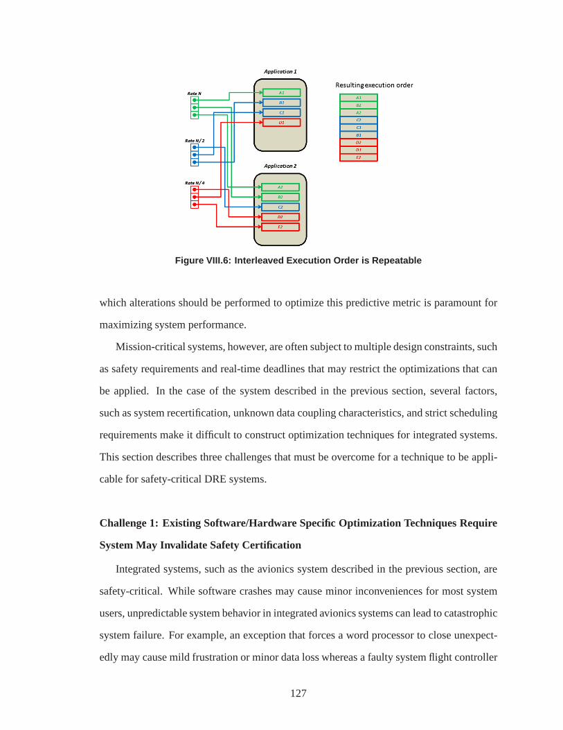
Figure VIII.6: Interleaved Execution Order is Repeatable

which alterations should be performed to optimize this predictive metric is paramount for

maximizing system performance.

Mission-critical systems, however, are often subject to multiple design constraints, such

as safety requirements and real-time deadlines that may restrict the optimizations that can

be applied. In the case of the system described in the previous section, several factors,

such as system recertification, unknown data coupling characteristics, and strict scheduling

requirements make it difficult to construct optimization techniques for integrated systems.

This section describes three challenges that must be overcome for a technique to be appli-

cable for safety-critical DRE systems.

Challenge 1: Existing Software/Hardware Specific Optimization Techniques Require

System May Invalidate Safety Certification

Integrated systems, such as the avionics system described in the previous section, are

safety-critical. While software crashes may cause minor inconveniences for most system

users, unpredictable system behavior in integrated avionics systems can lead to catastrophic

system failure. For example, an exception that forces a wordprocessor to close unexpect-

edly may cause mild frustration or minor data loss whereas a faulty system flight controller

127

could cause a passenger plane to crash. To ensure that these catastrophes will not occur, the

software and hardware components of safety-critical integrated avionics must be certified.

This certification guarantees that as long as the software and hardware are not modified,

the system will execute in a safe, predictable manner.

Existing cache optimization techniques such as loop fusionand data padding require

modifications to the components to increase cache utilization and performance [58, 87].

Modifications of system components, however, may void any previous safety certifica-

tions. Re-certification of system components can be a prohibitively slow and expensive

process, potentially resulting in dramatically increasedsystem cost and considerable devel-

opment delays. Therefore, techniques should be developed that alter the system to optimize

a predictive performance metric while leaving the hardwareand software of the system un-

modified. These techniques could increase system performance through better cache uti-

lization, resulting in decreased system runtime while avoiding the need for costly system

recertification.

Challenge 2: Data Sharing Characteristics of Software Components May Be Un-

known

As opposed to small, stand-alone software applications, integrated systems are com-

prised of several systems made up of many components workingtogether in concert. Sys-

tem developers usually work on a small portion of the components of a single system and

are unaware of the inner-workings of components developed by other manufacturers. For

example, the software that controls the system flight controller may consist of components

developed by a group in California and another in Texas, while the stabilizer may be de-

veloped by a different group exclusively in New Jersey. Therefore, system designers are

usually ignorant of amount of the implementation details ofthe software components that

may comprise the final system.

128

The data sharing characteristics of software can have a large impact on system perfor-

mance due to processor caching. However, system size may make data coupling analysis

excessively cumbersome and time consuming. Therefore, optimization techniques should

be developed to increase performance without requiring that the amount of data shared

between software be known a priori. These techniques could then be applied to systems

where the data coupling profile is unknown to increase the predictive performance metric

and ultimately reduce system execution time.

Challenge 3: Optimization Techniques Must Satisfy Real-time Scheduling Constraints

Safety-critical systems such as the avionics system described in the previous section

are subject to strict scheduling constraints. These systems commonly use a priority based

scheduling method, such as rate monotonic scheduling, to ensure that the software tasks

execute in a predictable manner [42,110]. For example, if a task A is assigned a priority of

rate N/2 and task B is assigned a priority of rate N, then task Bmust execute twice before

task A executes a second time. This ensures that tasks of higher priority will execute

without causing tasks of lower priority to completely starve due to continuous preemption.

Any optimization technique must result in a schedule that does not violate any of these

scheduling restrictions. This constraint prohibits many simple solutions that would greatly

increase the cache utilization but would also cause the system to behave in an unpredictable

and potentially catastrophic manner. This difficulty is compounded by the fact that the

priority of system tasks may fluctuate during system lifetime. Optimization techniques

should be developed that can be applied and re-applied when necessary to increase the

predictive performance metric and decrease system execution time for any set of system

task priorities.

129

Using SMACK to Evaluate and Adapt Integration Architecture s to Improve Cache

Performance

Each node of the system described in the case study consists of multiple partitions of

executing applications. The tasks that comprise these applications, as described in Sec-

tion VIII, are scheduled for execution with a priority-based scheduler that is specific to

each node. As tasks execute, cache hits may occur between tasks that share a common

partition. These cache hits can yield substantial reductions in the required execution time

of the partition.

Each of the partitions described in the case study is set to execute for a fixed-time

duration determined by the expected execution time for all tasks of the partition. This fixed-

time duration, however, does not take into account cache hits. Since execution time can be

substantially reduced if multiple cache hits occur, a segment of the fixed-time duration

of the partition could be spent idle, leading to wasted CPU cycles and decreased system

performance.

Goal: A Cache Hit Characterization Metric for Software Deployments

We propose the System Metric for Application Cache Knowledge (SMACK), for pre-

dicting the performance that a specific task scheduling willyield. SMACK can be used to

predict the performance for multiple execution schedules and to determine which schedule

will result in the greatest reduction of required executiontime. Further, using SMACK

can provide a much more accurate prediction of total execution time than techniques that

ignore potential cache hit benefits, leading to more efficient partition fixed-time durations.

SMACK Hypothesis

We expect that by profiling the data sharing of software tasksand creating an execution

schedule that decreases the occurrences of task executionsthat do not share data between

the execution of tasks that share data will increase temporal locality. We hypothesize that

130

altering the execution schedule of the software tasks of integrated applications to increase

temporal locality will result in increased cache hits and reduced system execution time

without violating real-time constraints.

How Real-time Schedules can Potentially Impact Cache Hits

As described in the case study, the physical structure of thesystem consists of multiple,

separate nodes. Each node is divided into separate partitions in which applications execute.

Each application executing in a partition is made up of tasksvarious rates and priorities.

Each node is equipped with a priority-based scheduler that determines the execution order

of these tasks. Different execution schedules can lead to more or less cache hits. While the

reduction in system execution time resulting from a successful cache hit may differ from

node to node, we assume it is the same for applications executing on a common node.

A task execution schedule is divided into frames and super-frames. A frame is a subset

of tasks that execute before the next set of tasks are allowedto begin executing. A super-

frame is the set of frames that must execute before all tasks of all rates will have executed.

For example, Figure VIII.6 shows an execution for a set of tasks. Tasks A1 through B1

execute in the same frame. The super-frame is the execution of all tasks from frame 0 to

frame 7.

Intra-frame Transitions

Transitioning between tasks executing in one or more framescan potentially result in a

cache hit. For example, Figure VIII.7 shows a scheduling of multiple tasks with six tasks

scheduled to execute in the same frame. Task A1 executes and then Task B2 is scheduled

to execute next. Since task A1 and B2 share the same frame, we call the transition from

A1 executing to B2 executing an intra-frame transition. If tasks A1 and B2 share common

require common data, then there is the potential for a cache hit.

131

Figure VIII.7: Scheduling with Intra-Frame Transitions

Extra-frame Transitions

Tasks may also be scheduled to execute in separate frames. A cache hit may result

from a transition from the final task to execute in one frame and the first task to execute

in the next frame. We call this type of this transition between separate frames an extra-

frame transition. For example, Figure VIII.8 shows two setsof tasks executing in separate

frames. An extra-frame transition exists between Task B1 and A1. The probability of a

cache hit occurring due to extra-frame and intra-frame transitions, however, differs based

on the cache contention factor.

Figure VIII.8: Scheduling with Extra-Frame Transition

132

Cache Contention Factor

Transitioning a new task onto the processor as described in Sections VIII and VIII

can result in a cache hit. However, the likelihood of a cache hit occurring as a result of

transition is based on the cache contention factor. The cache contention factor is defined as

the memory usage of the software, the size of the cache, and the cache replacement policy.

The cache contention factor determines how many different transitions can occur before all

the data written to the cache by a task is invalidated, reducing the probability of a cache hit

to 0.

For example, assume there are 5 applications consisting of 2tasks, each of which con-

sumes 2 kilobytes of memory of a 64k cache. The hardware uses aLeast Recently Used

(LRU) replacement policy in which the cache line that has remained the longest without

being read is replaced when new data is written to the cache. Executing the tasks will re-

quire writing 20 kilobytes to memory. Since the cache can store 64 kilobytes of data, all

data from all applications can remain in the cache. The cachecontention factor in this case

would be 10 since the last of the 10 tasks executed in the superframe could utilize the data

stored by the first task to execute in the superframe.

Now consider a system in which the total cache is only 2 kilobytes. Executing a task of

Application A would write 2 kilobytes of cache to memory, thereby filling the cache. Next,

a task of Application B executes writing 2 kilobytes of new data to the cache. Since the

cache is only 2 kilobytes, the cached data from the first task will be invalidated. Executing

a task from Application A will not result in cache hit since the cache data from the first task

was invalidated by the data of Application B written by the second task. In this case, two

tasks of the same application must execute consecutively toproduce cache hits. Therefore,

this set system would have a cache contention factor of 1.

133

Determining Total Cache Hits

Each intra-frame and extra-frame transition yields a probability of a cache hit based on

the contention factor of the system. Each of these cache hitswill reduce the execution time

of the system. The total probabilistic expected cache hits due to these transitions yields the

expected cache hits for this set of tasks. Adding the expected cache hits for all set of tasks

in all partitions of a given node will yield the total expected cache hits for the node.

The total execution time reduction for a node due to caching can be determined by

multiplying the total number of expected cache hits by the amount of time saved due to

successful cache hit, which may differ between nodes. Finally, the execution time reduc-

tion for a system can be determined by taking the sum of execution time reductions of all

nodes. In the following section, we formally define a methodology for determining the

total execution time savings due to caching of system deployments.

Defining and Calculating SMACK Cache Metric

Section VIII describes a high-level methodology for calculating the cache metric of a

system deployment. In this section, we will formally define this calculation. Please refer

to Section VIII for a higher level explanation as needed.

Calculating the Cache Contention Factor

The cache contention factor,CCF, determines how many consecutive transitions can

potentially lead to a cache hit before all cached data from the original task is invalidated.

CCF is calculated by dividing the size of the cache,CS, by the average amount of data

written per task. To determine the average amount of data written per task, the total amount

of data written,DW is divided by the number of tasks|T|, and multiplied by the percent of

task data shared between tasks,DS.

CCF=CS

((DW(T)/|T|)∗ (1−DS))(VIII.1)

134

FR(Fi j ,k) =

F(i−1)+(⌊ i+k|F| ⌋)(( j+k)%|F |) i +k< M(SF)

F(i−1)+(⌊

(i+k)−M(SF)|F | ⌋)((( j+k)−M(SF))%|F |)

i +k≥ M(SF)(VIII.4)

Determining if Tasks Overlap

In the integrated avionics system described in the case study, it is stated that tasks of

different applications do not share any data. Therefore, cache hits can only occur if two

tasks share the same application. Equation VIII.2 returns 1if two tasks are a part of the

same application and 0 if they are not.

O(ti, t j) =

1 ti == t j

0 ti! = t j

(VIII.2)

Quantifying Cache Hits for Variable Size Tasks

Software tasks of the same application may not read the same amount of memory. As

a result, the number of cache hits that result from a task executing will differ based on the

amount of common data read. Equation VIII.3 defines the maximum cache hits that can

be expected if a task of an application executes after another task of the same application.

The maximum cache hits is equal to the percentage of data shared by the tasks multiplied

by the amount of data read by the task executing later.

CHit(t(Fi) j , t(Fx)y) = DS∗DR(t(Fx)y (VIII.3)

Cache Hits due to Intra-frame & Extra-frame Transitions

We must calculate the cache hit probability "CHit" for all intra-frame and exta-frame

transitions in the superframe SF. The total set of transitions for a frame "F" is given by t(F).

Once a task executes, the number of transitions that can occur before all data written by the

135

TTot(SF) =|SF|−1

∑i=0

|F |−1

∑j=0

CCF−1

∑k=0

(CHit(t(Fi) j ,FR(t(Fi) j ,k)))

∗O(t(Fi) j ,FR(t(Fi) j ,k)) (VIII.5)

task to the cache is invalidated is determined by the CCF. Therefore, each transition that

occurs before the CCF is reached can potentially yield a cache hit and must be investigated.

Determining which task executesk transitions from a task is shown in Equation VIII.4.

We defineM(SF) as the number of tasks that execute in a given superframe. Twocases

must be considered: First, a task may executek steps ahead of a task, but in the same

superframe. This is shown in the first case of Equation VIII.4. Second, incrementing byk

transitions may exceed the boundary of the superframe. In this case, the task is determined

by wrapping back to the beginning of the superframe and incrementing any remaining

transitions as shown in the second case of Equation VIII.4.

Equation VIII.5 accounts for all cache hits due to all transitions in the superframe.

The first summation in Equation VIII.5 accounts for all frames in the superframe. The

second summation examines all frame transitions in the current frame. The innermost

summation in Equation VIII.5 sums the expected cache hits CHit for tasks that share the

same application, as given by O.

Total Cache Hits of a Partition

Each partition consists of one or more executing applications. To determine the total

expected cache hits for a given partition "(p)", the total expected cache hits of each appli-

cation "(a)" for each application "a" in the set of all applications "A" executing on partition

"p" must be summed as shown in Equation VIII.6.

θ(p) =|A|−1

∑k=0

β (ak) (VIII.6)

136

However, all tasks for a given partition will be executing inthe same super-frame "SF".

Therefore, the total number of caches hits due to all transitions in a super-frame will yield

the total cache hits for the set of applications in a partition, as shown in Equation VIII.7.

θ(p) =|A|−1

∑k=0

β (ak) = TTot(SF) (VIII.7)

Total Cache Hits of a Node

Cm(n) =Cc(n)∗|P|−1

∑j=0

θ(p j) (VIII.8)

Each node consists of one or more executing partitions. To calculate the cache benefits

"Cm(n)" of a single node "n", we must first determine the sum ofthe cache hits "(p)"

for each partition "p" from the set of all partitions "P" executing on node "n" as shown

in Equation VIII.8. This sum reflects the total probabilistic number of cache hits of the

partitions executing on the node.

Total Execution Time Reduction of a Node

The overhead execution time reduction resulting from a successful cache hit may differ

from node to node. We define this reduction as the Cache Constant or "Cc(n)". This value

must be supplied by the system designer or determined through profiling. Once we have

calculated the total number of cache hits on the node as described in 5.5 we multiply this

value by the Cc(n) to determine the total average overhead reduction (ms) for the node as

shown in Equation VIII.8.

Total Execution Time Reduction of a System

Finally, the physical structure of the system consists of multiple, separate nodes. To

quantify the total cache benefits (the total reduction of system overhead due to successful

137

cache hits) of the system, the cache benefits of each node mustbe calculated and summed.

This process is described in Equation VIII.9, which defines the SMACK metric "SMACK"

of a total set of nodes "N".

SMACK(N) =|N|−1

∑i=0

Cm(ni) (VIII.9)

Notation Quick Reference Guide

• Cm(N) is the Cache Metric, or the expected probabilistic amount of time(ms) saved

through cache effects for all N.

• N is the set of hardware processing nodes.

• SMACK(N) predicts the performance of the set of processingnodes N.

• O(ti, t j) returns 1 if the tasks are of the same application and 0 if not.

• M(SF) as the number of tasks that execute in a given superframe.

• Cm(n) is the expected probabilistic amount of time saved through cache effects for a

single node n.

• Cc(n) is the amount of time(ms) that each cache hit saves on agiven node n. âAS P

is the set of partitions for a given node n.

• θ (p) total number of expected cache hits for all applicationsA in a given partition p.

• β (a) is the total number of expected cache hits for all tasks T in a given application

a.

• Fi ∈ F is the set of tasks that execute in the ith frame.

• CHit(Ti,Tj) returns the probabilistic number of cache hits that will occur when exe-

cuting Ti immediately before Tj.

138

• SF, called a super-frame, is the set of frames that execute before the last task of

the lowest priority executes. This set includes the frame that the last task of lowest

priority executes in.

• CS, is the size of the processor cache.

• T is the set of all software tasks to execute.

• DS is the average percentage of application member variables read that are shared

between tasks, i.e. if all tasks read the same variables thenDS is 1.

• DW(T) is the total amount of data written to the cache by all tasks.

• CCC, called the Cache Contention Metric, uses the cache size, CS, number of tasks,

• TTot(SF) is the total number of cache hits due to extra-frame and intra-frame transi-

tions for super-frame SF.

Applying the SMACK Metric to Increase System Performance

This section describes how SMACK can be applied to potentially increase cache hit rate

while resolving the challenges described in the section entitled “Challenges of Predictive

Performance Analysis of Integrated Systems”. The SMACK metric is used as a heuristic

to determine the “score” of potential system configurations. For instance, if calculating

the SMACK metric for system A yields a higher score than doingthe same for system B,

then we assume that executing system A will result in a fasterexecution time due to more

efficient data caching.

To determine if SMACK can be applied to reduce the runtime of integrated systems

by increasing the cache hit rate, we examine an instance of the avionics system described

in the case study. Due to the challenges described in the section entitled “Challenges of

Predictive Performance Analysis of Integrated Systems”. specifically Challenge 1, cache

optimization techniques that alter the software of the system cannot be applied. Therefore,

139

we must determine if there are other ways to optimize the SMACK value of the system

without modifying the underlying software, altering the data coupling characteristics of the

software, and while meeting all real-time scheduling requirements.

As discussed in the case study, multiple tasks schedules exist that satisfy real-time

scheduling requirements. As stated in Section VIII, many existing cache optimization

methods require altering the software, which then requiresexpensive and time consuming

recertification. Changing the execution ordering of the tasks, however,does notactually

alter the software and therefore does not require recertification. The SMACK score of one

task ordering may be greater than that of others, thereby indicating a faster runtime.

Fortunately, it is extremely unlikely that the SMACK score will be the same for all

task schedules. As specified in the system defined in the case study, tasks of different

applications do not share data. The Cache Contention Factor(CCF) determines how many

task executions of other applications can occur after a taskexecutes before the cache is

potentially completely invalidated.

As a result, executing tasks of the same application consecutively will lower the SMACK

metric and therefore execution time, despite having limited or no knowledge of the data

coupling between tasks, as stated in Challenge 2. If more is known about the data coupling

characteristics of the tasks between common applications,the more accurate the SMACK

value will be.

Finally, reordering the tasks to attempt to increase the SMACK value of the system

cannot be done in a haphazard fashion. Any execution order must adhere to the real-time

scheduling constraints defined in Challenge 3. This greatlyrestricts the total potential

execution orders that satisfy all system constraints. Scheduling techniques, such as rate

monotonic scheduling, can be applied to create schedules that enforce real-time constraints.

140

Empirical Results

This section presents an analysis of the performance of multiple systems with different

SMACK values. These systems differ in task execution schedules and the amount of mem-

ory shared between tasks. For each system, we investigate potential correlations between

the SMACK score and L1 cache misses, L2 cache misses, and runtime reductions.

To examine the relationship between SMACK score and system performance, we were

required to create multiple software systems to mimic the scale, execution schedule and

data sharing of the system described in the case study. For each system, we specified the

number of applications, number of tasks per application, the distribution of task priority,

and the maximum amount of memory shared between each task. Wecreated a Java based

code generator to create C++ system code that possessed these characteristics. Rate mono-

tonic scheduling was used to create a deterministic priority based schedule for the generated

tasks that adheres to rate monotonic scheduling requirements.

Figure VIII.9: Processor Instructions Profiled with VTune

Experimental Platform

The systems were compiled and executed on a Dell Latitude D820 with a 2.16Ghz

Intel Core 2 processor with 2 x 32kb L1 instruction caches, 2 x32 kb write-back data

caches, a 4 MB L2 cache and 4GB of RAM running Windows Vista. For each experi-

ment, each system was executed 50 times to obtain an average runtime. These executions

were profiled using the Intel VTune Amplifier XE 2011. VTune isa profiling tool that is

141

capable of calculating the total number of times an instruction is executed by a proces-

sor. For example, to determine the L2 cache misses of System ’A’, System ’A’ is com-

piled and then executed with VTune configured to return the total times that the instruction

MEM_LOAD_REQUIRED.L2_MISS is called. Figure VIII.9 showsthe instructions that

were profiled in the following experiments as well as their semantic meanings.

Creation Process of Simulated Systems

To test the SMACK based schedule modification technique, we created a software suite

for generating the C++ code of mock integrated avionics systems that behave as specified in

the case study. As shown in Figure VIII.10, these systems include a priority based scheduler

and multiple sample avionics applications consisting of a variable number periodic avionic

tasks.

Figure VIII.10: System Creation Process

Together, these components comprise a full test avionics system. The data sharing and

memory usage of these applications as well as the schedulingtechnique are all parame-

terized and varied to generate a range of test systems. We usethese simulated systems to

validate the SMACK metric by showing that a higher SMACK value correlates with better

performance in terms of execution time and cache misses.

142

Data Sharing Characteristics

The data shared between applications and shared between tasks of the same application

can greatly impact the cache effectiveness of a system. For example, the more data that is

shared between two applications, the more likely that the data in the cache can be utilized

by tasks of the applications, resulting in reduced cache misses and system runtime. The

integration architecture described in the case study prohibits data sharing between tasks of

different applications. Therefore, all systems profiled inthis section are also restricted to

sharing data between tasks of the same application.

Task Execution Schedule

The execution schedule of the software tasks of the system can potentially affect system

performance. For example, assume there are two applications named App1 and App2 that

do not share data. Each application contains 1000 task methods, with tasks of the same

application sharing a large amount of data. The execution ofa single task stores enough

memory to completely overwrite any data in the cache, resulting in a Cache Contention

Factor of 1. A task from App1 executes, completely filling thecache with data that is only

used by App1. If the same or another task from App1 executes next, data could reside in

the cache that could potentially result in a cache hit. Sinceno data is shared with App2,

however, executing a task from App2 could not result in a cache hit and would overwrite all

data used by App1 in the class. Therefore, multiple execution schedules effect performance

differently and produce different SMACK scores.

Experiment 1: Variable Data Sharing

As stated in the section entitled “Data Sharing Characteristics”, the amount of data

shared between multiple tasks can potentially have a large impact on the performance of a

system in terms of cache misses and system runtime. To examine the effect of data sharing

between tasks of common applications, we constructed 10 software systems. Each of these

143

systems contained 5 separate applications consisting of ten tasks each. The body of the

tasks consisted of floating and integer addition operations. The total number of operations

of the tasks was constant across all applications.

Figure VIII.11: Amount of Data Shared vs Runtime.

The amount of data shared between the same tasks, however, was manipulated. For

example, if the data sharing between tasks was set to 20%, then each tasks shared ap-

proximately 20% of the variables used in operations with allother tasks. After generating

these ten software systems, we executed each system 50 timesand determined an average

runtime of each system.

As can be seen in Figure VIII.11, as the amount of data shared between tasks of a single

application, the faster the system can execute. In this case, sharing 100% of data resulted in

an execution time of 2572.58 milliseconds, where as a sharing of no data between tasks, or

0%, resulted in an execution time of 3704.85 milliseconds, which is a difference of 30.56%.

It is important to note, however, that the curve shown in Figure VIII.11 is non-linear, with

only an additional reduction of 9.40% occurring as a result of increasing the shared data

amount from 50% to 100%.

Increasing the amount of shared data between tasks also leads to a decrease in cache

misses. As described in the section entitled “ExperimentalPlatform” VTune Amplifier

144

Figure VIII.12: Amount of Data Shared vs L2 Cache Misses

XE 2011 was used to determine the total number of L2 and L1 cache misses by moni-

toring for MEM_LOAD_RETIRED.L2_MISS” and MEM_LOAD_RETIRED.L1D_MISS

instructions. It is important to note that these instructions only take into account cache

misses due to data write-back and do not include cache missesresulting from instruction

fetching.

Figure VIII.12 shows the number of L2 cache misses as data sharing between tasks

increases. As the data sharing increases the number of L2 cache misses decrease at an

exponential rate. In this case from 5.172x108 to 1.6x105 a reduction of 99.69%. As with

runtime, the vast majority of L2 cache miss reductions occurred by increasing the amount

of shared data from 0 %to 50% or greater, resulting in an 80.36% L2 cache miss reduc-

tion. Figure VIII.13 shows the number of L1 cache misses decrease as data between tasks

increases. In contrast to runtime and L2 cache misses, the decrease in L1 cache misses is

considerably more linear.

Experiment 2: Execution Schedule Manipulation

As discussed in the section entitled “Task Execution Schedule”, the execution schedule

of tasks can potentially impact both the runtime and number of cache misses of a system.

In this experiment, we manipulated the execution order of a single software system with

145

20% shared data probability between 5 applications consisting of 10 tasks each to create 4

new execution schedules.

Figure VIII.13: Amount of Data Shared vs L1 Cache Misses

First, stride scheduling was used to create an execution ordering that meets all schedul-

ing constraints. This schedule was then permuted to change the total number of instances

in which the execution of two tasks from a common applicationexecuting could poten-

tially cause a cache hit, referred to as "overlaps". The number of overlaps that exist in an

execution schedule is effected by the number of task executions that must occur before the

amount of data written to the cache exceeds the size of the cache, defined by the Cache

Contention Factor. For example, if each task writes 30k to memory and the cache size is

50k, then most data written to the cache by the first task executing would persist through

the execution of two more tasks. Therefore, the Cache Contention Factor for this system

would be two.

The original execution schedule generated by Stride Scheduling is referred to as "Un-

optimized”. The Cache Contention Factor for the experimental platform was 15, thereby

yielding 655 overlaps for the Unoptimized schedule. This schedule was then permuted

to increase the number of overlaps while satisfying priority scheduling constraints. This

schedule is referred to as the "Optimized" ordering and it contained 801 overlaps.

We also created two execution schedules that do not satisfy the priority scheduling

146

Figure VIII.14: Runtimes of Various Execution Schedules

requirement to maximize and minimize the number of overlaps. To minimize the number

of overlaps, we permuted the execution order such that no twotasks of the same application

executed consecutively, resulting in the "Worst" case execution order with 732 overlaps.

Figure VIII.15: Cache Contention Factor vs Overlaps

We refer to this execution order as the Worst execution orderas it yields 0 overlaps

when the Cache Contention Factor is one. As shown in Figure VIII.15, as cache size in-

creases, the Worst execution order may result in more overlaps than other execution orders.

Finally we maximized the number of overlaps by executing alltasks of each application

consecutively, resulting in 1743 overlaps. We refer to thisexecution ordering as the "Best"

execution schedule.

The average runtimes for the different execution schedulescan be seen in Figure VIII.14.

147

Figure VIII.16: Execution Schedules vs L1 Cache Misses

As can be seen, the task execution order can have a large impact on runtime. In this case,

the Best execution schedule, consisting of 1743 overlaps, executed in 2790 milliseconds on

average. The Optimized execution schedule completed in 3299 milliseconds, an 18.24% in-

crease from the Best execution schedule. The Unoptimized and Worst execution schedules

executed in 3337 and 3329 milliseconds respectively.

Execution order was also shown to impact the number of cache misses. Figure VIII.16

shows the L1 cache misses for all execution schedules. Once again, the execution schedule

with the most overlaps, Best, performed the best of all execution orders, resulting in only

3.2584x109 cache misses. The Optimized execution schedule, consisting of 801 overlaps,

generated 3.484x109 cache misses, an increase of 6.47% from the L1 cache misses ofthe

Best execution order. Next, the Unoptimized execution schedule, consisting of 655 over-

laps, resulted in 3.5076x109 L1 cache misses. Finally, the Worst execution order resulted

in 3.5336x109 L1 cache misses, the most of all execution orders.

The impact of execution order on L2 cache misses can be seen inFigure VIII.17. Simi-

larly to L1 cache misses and runtime, the execution schedulewith the most overlaps, Best,

produced the lowest results with 1.588x108 L2 cache misses. The Worst case execution

schedule generated less L2 cache misses than the Unoptimized schedule which in turn gen-

erated less L2 cache misses than the Optimized schedule.

148

Figure VIII.17: Execution Schedules vs L2 Cache Misses

Experiment 3: Dynamic Execution Order and Data Sharing

The section entitled “Data Sharing Characteristics” and Experiment 2 demonstrate the

effects of the data sharing characteristics of applications and execution order of tasks on

runtime and cache misses. These sections, however, do not examine the impact of altering

both of these aspects concurrently. In this section we examine multiple execution orders

for multiple systems with different data sharing characteristics. For example, the reduction

in system cache misses could be substantially different by altering the execution order of a

system with 80% shared data than a system with only 10% shareddata.

The number of L1 cache misses also decreases as the number of overlaps in the execu-

tion order and/or the amount of shared data increases as shown in Figure VIII.19. Again,

the Best execution order consisting of the most overlaps resulted in the fewest L1 cache

misses for all software systems. Unlike runtime, however, the number of L1 cache misses

are only slightly less than those of the other execution orders. Further, L1 cache misses for

all execution orders decreased at near-linear rate.

As can be seen in Figure VIII.20, however, L2 cache misses decreased at an exponential

rate. Once again, the Best execution order resulted in the lowest number of cache misses

for almost all trials, with the exception of the system with 90% data sharing in which the

number of L2 cache misses were comparably negligible. The exponential nature of the

decrease in cache misses show that the greatest reduction inL2 cache misses can be made

149

by altering increasing the total amount of shared data if less than 50% of data is shared.

For example, increasing the amount of data shared from 0% to 50% for the Optimized

execution order resulted in an L2 cache miss reduction of 77.64%. Increasing data sharing

from 50% to 90%, however, does not yield as extreme benefits. Increasing the amount of

data shared from 50% to 90% for the Optimized execution orderresulted in an additional

reduction of only 21.18%.

Figure VIII.18: Runtime vs Data Shared and Execution Order

As can be seen in Figure VIII.18, system execution time decreases as the amount of

shared data increases. However, the decrease in runtime is not constant across all execution

orders. For example, the Best execution order decreases from 2884 milliseconds when 0%

of data is shared to 2398 milliseconds when 100% of data is shared, a total decrease of 486

milliseconds or 16.85%. The Optimized execution order decreases from 3592 milliseconds

to 2582 milliseconds as the shared data increase from 0% to 100%, for a total runtime

decrement of 1010 milliseconds or 28.12%. Altering the amount of data shared reduced

the system runtime of the Optimized execution order by 107.82% more than the same data

alteration with the Best optimized execution order. Therefore, it can be seen that altering

the amount of data shared has a larger impact on runtime for systems with less efficient

execution orders.

While adjusting the data sharing characteristics of a system may be acceptable at design

150

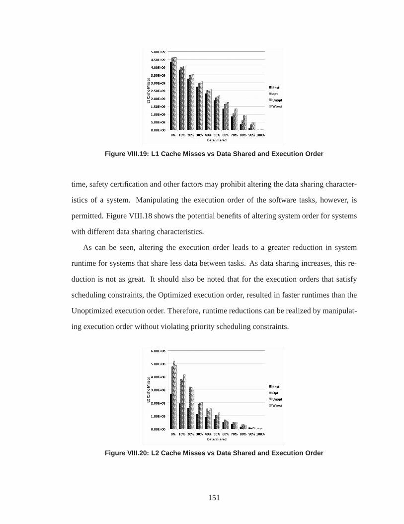
Figure VIII.19: L1 Cache Misses vs Data Shared and Execution Order

time, safety certification and other factors may prohibit altering the data sharing character-

istics of a system. Manipulating the execution order of the software tasks, however, is

permitted. Figure VIII.18 shows the potential benefits of altering system order for systems

with different data sharing characteristics.

As can be seen, altering the execution order leads to a greater reduction in system

runtime for systems that share less data between tasks. As data sharing increases, this re-

duction is not as great. It should also be noted that for the execution orders that satisfy

scheduling constraints, the Optimized execution order, resulted in faster runtimes than the

Unoptimized execution order. Therefore, runtime reductions can be realized by manipulat-

ing execution order without violating priority schedulingconstraints.

Figure VIII.20: L2 Cache Misses vs Data Shared and Execution Order

151

Experiment 4: Predicting Performance with SMACK

The previous experiments demonstrate the impact of the datasharing and execution

schedule of several different systems. This section examines the correlation between the

SMACK score and actual runtime for a system. As described in the section entitled “Eval-

uating Systems for Expected Cache Hits with SMACK”, SMACK uses the execution order

and data sharing characteristics in conjunction with a Cache Contention Factor to score

systems in terms of expected performance. SMACK provides a basis for comparing mul-

tiple systems in terms of expected performance. For example, if System ’A’ produces a

higher SMACK score than System ’B’ then System ’A’ is expected to have a faster runtime

for System ’B’.

Figure VIII.21: Smack Score vs Data Shared and Execution Ord er

Experiment 3 presents 44 different systems with data sharing ranging from 0%-100%

and four different execution schedules for each. Each system was executed on the same

hardware, thereby producing the same value for the contention factor. The SMACK value is

calculated for each system taking into account the contention factor, the execution schedule,

and data sharing characteristics.

Figure VIII.21 presents the SMACK values for each system. Asthe amount of data

sharing increases, the SMACK score increases, indicating areduction in runtime. Compar-

ing the SMACK scores shown in Figure VIII.21 to the actual system execution times shown

152

in Figure VIII.18 shows that the a higher SMACK score does correlates with a decrease in

execution time. Similarly to runtime, optimizing the execution schedule of a system is

also shown to reduce the SMACK score. Therefore, the SMACK metric is effective for

predicting and comparing the performance of multiple software systems.

Experiment 2 presents four different execution schedules used to execute the software

systems tested. Of these execution schedules, only the Unoptimized and Optimized exe-

cution schedules satisfy priority based scheduling constraints. The Unoptimized schedule

was built without taking into account the effect of overlapson system performance. The

Optimized execution order is created by reordering the tasks executions such that overlaps

are increased without violating priority scheduling constraints.

Figure VIII.22 shows the percentage reduction in runtime bychanging the unoptimized

execution order to increase overlaps and create the Optimized execution order. Altering the

execution order resulted in an average runtime reduction of2.4% though was shown to be

as high as 4.34%. This reduction can be realized without altering the underlying hardware

or software executing on the system. Therefore, optimizingsystem execution schedules

to minimize SMACK scores can lead to substantial reductionsin system execution time

without requiring extensive knowledge of the software, access to the code, recertification,

or alterations to the hardware.

Figure VIII.22: Percent Runtime Reduction vs Data Shared

153

It should be noted that the Optimized execution order presented here is not theoptimal

execution order that would lead to the maximum smack score. Even for systems with the

same software, the hardware can have a large impact on the Cache Contention Factor, which

is an integral part of the SMACK score calculation. Experiment 2 demonstrates that the

Cache Contention Factor of a system changes the effectiveness of an execution schedule.

In future work, we investigate creating an algorithmic technique that takes into account

the Cache Contention Factor of a system to maximize the SMACKscore and performance

gains.

154

CHAPTER IX

CONCLUDING REMARKS

This chapter presents lessons learned from our work in DRE system deployment and

configuration derivation. Chapter 2 presents our findings from constructing an automated

technique for deriving deployments with reduced processorrequirements. Chapter 3 show-

cases conclusions drawn from creating a tool to optimize system-wide deployment proper-

ties. Chapter 4 describes lessons learned from creating a model-driven tool for DRE system

configuration. Chapter 5 presents our discoveries from creating an automated technique for

evolving DRE systems. Chapter 6 provides a model-driven technique for reducing oper-

ating cost and emissions of cloud computing environments. Finally, Chapter 7 presents

the SMACK metric for assessing and predicting the performance gains of systems due to

processor caching.

Automated Deployment Derivation

Determining component deployments that minimize the number of required processors

is hard. This problem is exacerbated by proving that software applications are schedula-

ble for a chosen deployment. Using bin packing algorithms, such as first-fit decreasing,

the entire deployment space need not be searched. By using our BLITZ algorithm (which

combines first-fit decreasing bin packing with proven utilization bounds based on data char-

acteristics), valid and near minimal deployments can be determined.

Based on our work with BLITZ thus far, we learned the following lessons pertaining to

deployment for DRE systems:

• Grouping based on harmonic periods improves packing tightness. BLITZ com-

bines the Liu-Layland equation with the increased utilization bound of components

155

with harmonic execution periods to maximize the utilization of each processor dur-

ing deployment. As a result, tasks can be clustered on fewer processors, reducing the

processors required.

• Processor minimization depends on real-time benchmarks. BLITZ has been

shown to greatly reduce the required processors of a DRE system of an extensively

benchmarked real-time system. Without knowledge of periodicity, resource con-

straints, and co-location constraints, BLITZ cannot be fully utilized. It is essential

to develop tools that effectively simulate and thoroughly benchmark DRE systems

before they are deployed so that the full capabilities of BLITZ can be applied.

The current version of BLITZ with example code is available in open-source form at

ascent-design-studio.googlecode.com. The industry challenge problem that

is the basis for this chapter can be found atwww.sprucecommunity.org.

Legacy Deployment Optimization

Optimizing deployment topologies on legacy embedded flightavionics system can yield

substantial benefits, such as reducing hardware costs and power consumption. By combin-

ing the efficiency of metaheuristic optimization techniques (such as particle swarm opti-

mization) with other heuristic algorithms (such as bin-packing) legacy deployments can be

evolved and optimized in a matter of seconds.

The following are a summary of the lessons we learned applying our ScatterD tool for

deployment optimization to a legacy flight avionics system:

• Multiple constraints make deployment planning hard. Avionics deployments

must adhere to a wide range of strict constraints, such as resource, colocation, schedul-

ing, and network bandwidth. Deployment optimization toolsmust account for all

these constraints when determining a new deployment.

156

• A Huge deployment space requires intelligent search techniques. The vast ma-

jority of potential deployments that could be created violate one or more design con-

straints. Intelligent and automated techniques, such as hybrid-heuristic bin-packing,

should therefore be applied to discover valid “near-optimal” deployments.

• Substantial processor and network bandwidth reductions are possible.Applying

hybrid-heuristic bin-packing to the flight avionics systemresulted in 42.8% proces-

sor reduction and 24% bandwidth reduction. Our future work is applying hybrid-

heuristic bin-packing to other embedded system deploymentdomains, such as auto-

mobiles, multi-core processors, and tactical smartphone applications.

The ScatterD tool is available in open-source form in the Ascent Design Studio(ascent-design-studio.

googlecode.com). A document describing the flight avionics system case study as well

as additional information on ScatterD, can be found at the SPRUCE web portal (www.

sprucecommunity.org), which pairs open industry challenge problems with cutting-

edge methods and tools from the research community.

Model Driven Configuration Derivation

Determining valid configurations for distributed real-time and embedded (DRE) sys-

tems is hard. Designers must take into account a myriad of constraints including resource

constraints, real-time constraints, QoS constraints, andother functional constraints. The

difficulty of this task is exacerbated by the presence of a plethora of potential COTS com-

ponents for inclusion in the configuration, with each providing varying quality of service,

functionality, resource requirements and financial cost. This high availability of COTS

components results in an exponential number of potential DRE system configurations.

As a result, manual techniques for determining valid DRE system configurations are

far too cumbersome. Even exact automated techniques, such as the use of CSPs, require

a prohibitive amount of time to execute. Approximation techniques, such as ASCENT,

157

however, do not require an exhaustive search of the vast design space allowing a much

more rapid execution while often resulting in solutions with over 95% optimality.

The use of complex programmatic techniques in approximation techniques like AS-

CENT often have a steep learning curve and require large amounts of coding to construct

a problem for execution. Due to the complex coding involved,these techniques carry the

added burden of being error prone when defining problem instances. To address these chal-

lenges, an MDA-based tool called the Ascent Modeling Platform (AMP) that utilized GME

to construct problem instances and display valid solutionsfor DRE system configurations

was utilized. The following are lessons learned during our creation and use of AMP:

• Modeling tools provide rapid problem construction. Through the use of GME,

problems could be constructed in a fraction of the time of using programmatic tech-

niques.

• Utilizing MDA reduces human error. AMP utilizes a GME metamodel that en-

forces the many complex design constraints associated withDRE system configu-

ration. As a result, users of AMP are prevented from constructing a configuration

problem that is invalid.

• Modeling tools facilitate design space exploration.Solutions are posted directly

back into the model for analysis by system designers. Designers can then change

problem parameters within the model and execute the interpreter to explore multiple

configuration scenarios, resulting in an increased understanding of the design space.

• Multiple execution options still needed.Currently ASCENT is the only technique

that is executed upon interpreting models in AMP. Other techniques, such as the use

of CSP solvers, should be implemented to determine solutions to problems with an

appropriately reduced number of candidate components.

The current version of AMP with example code is available in open-source form at

ascent-design-studio.googlecode.com.

158

Automated Hardware and Software Evolution Analysis

It is hard to determine valid DRE system evolution configurations that increase DRE

system value. The exponential number of possible configurations that stem from the mas-

sive variability in these problems prohibit the use of exhaustive search algorithms for non-

trivial problems. This chapter presented theSoftware Evolution Analysis with Resources

(SEAR) technique, which converts common evolution problems into multi-dimensional

multiple-choice knapsack problems(MMKP). We also empirically evaluated three differ-

ent algorithms for solving these problems to compare their effectiveness in providing valid,

high-value evolution configurations.

From these experiments, we learned the following lessons pertaining to determine valid

evolution configurations for hardware/software co-designsystems:

• Approximation algorithms scale better than exhaustive algorithms. Exhaustive

search techniques, such as the linear constraint solver algorithm, cannot be applied to

non-trivial problems. The determining factor in the effectiveness of these algorithms

is the number of problem sets. To solve problems with realistic set counts in feasible

time, approximation algorithms, such as the M-HEU algorithm or the ASCENT al-

gorithm must be used. These techniques can solve even large problems in seconds,

with minimal impact on optimality.

• Extremely small or large problems yield near-optimal solutions. For non-trivial

problems, the ASCENT algorithm and M-HEU algorithm can be used to determine

near-optimal evolution configurations. For tiny problems,the LCS algorithm can be

used to determine optimal solutions. Given that these tiny problems have few points

of variability, optimal solutions can be determined rapidly.

• Problem size should determine which algorithm to apply.Based on problem char-

acteristics, it can be highly advantageous to use one algorithmic technique versus

another, which can result in faster solving times or higher optimality. Figure VI.15

159

shows the problem attributes that should be examined when deciding which algo-

rithm to apply. It also relates the algorithm that is best suited for solving these evo-

lution problems based on the number of sets present.

• No algorithm is universally superior. The analysis of empirical results indicate

that all three algorithms are superior for different types of evolution problems. We

have not, however, discovered an algorithm that performs well for every problem

type. To determine if other existing algorithms perform better for one or all types

of evolution problems, further experimentation and analysis is necessary. Our future

work will therefore examine other approximation algorithms, such as evolutionary

algorithms [6, 39] and particle swarm techniques [57, 101],to determine if a single

superior algorithm exists.

The current version of ASCENT with example code that utilizes SEAR is available in

open-source form atascent-design-studio.googlecode.com.

Virtual Machine Configuration & Auto-scaling Optimization

Auto-scaling cloud computing environments helps minimizeresponse time during pe-

riods of high demand, while reducing cost during periods of light demand. The time to

boot and configure additional VM instances to support applications during periods of high

demand, however, can negatively impact response time. Thischapter describes how the

Smart Cloud Optimization of Resource Configuration Handling (SCORCH) MDE tool uses

feature models to (1) represent the configuration requirements of multiple software applica-

tions and the power consumption/operational costs of utilizing different VM configurations,

(2) transform these representations into CSP problems, and(3) analyze them to determine

a set of VM instances that maximizes auto-scaling queue hit rate. These VM instances

are then placed in an auto-scaling queue so that response time requirements are met while

minimizing power consumption and operational cost.

160

The following are lessons learned from using SCORCH to construct auto-scaling queues

that create greener computing environments by reducing emissions resulting from super-

fluous idle resources:

• Auto-scaling queue optimization effects power consumption and operating cost.

Using an optimized auto-scaling queue greatly reduces the total power consump-

tion and operational cost compared to using a statically provisioned queue or non-

optimized auto-scaling queue. SCORCH reduced power consumption and operating

cost by 50% or better.

• Dynamic pricing options should be investigated.Cloud infrastructures may change

the price of procuring VM instances based on current overallcloud demand at a given

moment. We are therefore extending SCORCH to incorporate a monitoring system

that considers such price drops when appropriate.

• Predictive load analysis should be integrated.The workload of a demand model

can effect application resource requirements drastically. We are therefore extending

SCORCH to use predictive load analysis so auto-scaling queues can cater to specific

application workload characteristics.

SCORCH is part of the ASCENT Design Studio and is available inopen-source format

from code.google.com/p/ascent-design-studio.

Predictive Processor Cache Analysis

Processor data caching can substantially increase DRE system performance and reduce

system runtime. Several factors, such as task execution schedule, data sharing characteris-

tics, and system hardware can influence the caching effects of a system, making it difficult

to predict performance gains. Without a formal methodologyfor predicting performance

gains due to the processor caching behavior of a system, it isextremely difficult to compare

multiple potential system implementations or apply performance optimizations.

161

This paper presents the System Metric for Application CacheKnowledge (SMACK) for

quantifying the performance gains of processor caching of asystem. System performance

of multiple system implementations can be assessed and compared based on SMACK

score. The system with the lowest SMACK score will better utilize the processor cache

than other system implementations, resulting in decreasedsystem execution time. Further,

certain aspects of the systems could potentially be altered, such as execution schedule, to

optimize the SMACK score and decrease system execution time. We empirically evalu-

ated applying the SMACK metric to 44 different simulated industry avionics system to

determine if a correlation exists between the SMACK metric and runtime reductions due

to processor caching.

As a result of these efforts, we learned the following lessons from predicting the impact

of processor caching on system performance

• Both hardware and software design decisions effect the SMACK score of a sys-

tem. The processor cache size, data sharing characteristics andtask execution have a large

impact on the SMACK score. The SMACK score tends to improve with increases in cache

size and data sharing. The execution order of system task effects the SMACK score differ-

ently based on the cache contention factor.

• Decreases in the SMACK score correlates with increased system performance

and decreased system execution time.Increasing the data sharing and/or altering the

execution order of a system leads to a decreased SMACK score.Reducing the SMACK

score correlated with an average runtime reduction of 2.4%.Therefore, multiple system

implementations can be compared based on their SMACK scores.

• Effects of other cache replacement policies should be investigated. The SMACK

metric does not take into account the cache replacement policy of a system and was only

tested with random replacement policy. The effectiveness of SMACK should be investi-

gated for other cache policies, such as Least Recently Used (LRU) and First In First Out

(FIFO).

162

• Algorithmic techniques to maximize SMACK should be developed. The execution

order of tasks was shown to have a large impact on system performance and SMACK score.

Further, the performance of execution schedules differed base on the Cache Contention

Factor. In future work, we will examine the development of algorithmic techniques that

use SMACK and the Cache Contention Factor as a heuristics fordetermining the optimal

execution order for the tasks of specific systems.

163

BIBLIOGRAPHY

[1] Computer Center PowerNap Plan Could Save 75 Percent Of Data Cen-ter Energy. http://www.sciencedaily.com/releases/2009/03/090305164353.htm, 2009. Accessed October 20, 2010.

[2] G. Abandah and A. Abdelkarim. A Study on Cache Replacement Policies. 2009.

[3] M.M. Akbar, E.G. Manning, G.C. Shoja, and S. Khan. Heuristic Solutions for theMultiple-Choice Multi-dimension Knapsack Problem.Lecture Notes in ComputerScience, pages 659–668, 2001.

[4] J.R. Allen and K. Kennedy. Automatic loop interchange. In Proceedings of the 1984SIGPLAN symposium on Compiler construction, page 246. ACM, 1984.

[5] C. Alves and J. Castro. Cre: A systematic method for cots components selection. InXV Brazilian Symposium on Software Engineering (SBES). Rio de Janeiro, Brazil,2001.

[6] T. Bäck. Evolutionary Algorithms in Theory and Practice: EvolutionStrategies,Evolutionary Programming, Genetic Algorithms. Oxford University Press, USA,1996.

[7] R.I. Bahar, G. Albera, and S. Manne. Power and performance tradeoffs using variouscaching strategies. InLow Power Electronics and Design, 1998. Proceedings. 1998International Symposium on, pages 64–69. IEEE, 2005.

[8] A. Bateman and M. Wood. Cloud computing.Bioinformatics, 25(12):1475, 2009.

[9] D. Batory. Feature Models, Grammars, and PrepositionalFormulas.Software Prod-uct Lines: 9th International Conference, SPLC 2005, Rennes, France, September26-29, 2005: Proceedings, 2005.

[10] Hakem Beitollahi and Geert Deconinck. Fault-TolerantPartitioning Scheduling Al-gorithms in Real-Time Multiprocessor Systems.Pacific Rim International Sympo-sium on Dependable Computing, IEEE, 0:296–304, 2006.

[11] A. Beloglazov and R. Buyya. Energy efficient allocationof virtual machines incloud data centers. InCluster, Cloud and Grid Computing (CCGrid), 2010 10thIEEE/ACM International Conference on, pages 577–578. IEEE, 2010.

[12] D. Benavides, P. Trinidad, and A. Ruiz-Cortes. Automated Reasoning on Fea-ture Models. 17th Conference on Advanced Information Systems Engineering(CAiSEŠ05, Proceedings), LNCS, 3520:491–503, 2005.

164

[13] D. Benavides, P. Trinidad, and A. Ruiz-Cortés. Automated reasoning on featuremodels. InLNCS, Advanced Information Systems Engineering: 17th InternationalConference, CAiSE 2005, volume 3520, pages 491–503. Springer, 2005.

[14] David Benavides, Pablo Trinidad, and Antonio Ruiz-Cortes. Automated Reasoningon Feature Models. InProceedings of the 17th Conference on Advanced InformationSystems Engineering, Porto, Portugal, 2005. ACM/IFIP/USENIX.

[15] A. Berl, E. Gelenbe, M. Di Girolamo, G. Giuliani, H. De Meer, M.Q. Dang,and K. Pentikousis. Energy-efficient cloud computing.The Computer Journal,53(7):1045, 2010.

[16] A.A. Bertossi, L.V. Mancini, and F. Rossini. Fault-Tolerant Rate-Monotonic First-Fit Scheduling in Hard-Real-Time Systems.IEEE Transactions On Parallel andDistributed Systems, pages 934–945, 1999.

[17] K. Beyls and E. DùHollander. Reuse distance as a metric for cache behavior. InProceedings of the IASTED Conference on Parallel and Distributed Computing andsystems, volume 14, pages 350–360. Citeseer, 2001.

[18] B. Boehm, B. Clark, E. Horowitz, C. Westland, R. Madachy, and R. Selby. Costmodels for future software life cycle processes: COCOMO 2.0. Annals of SoftwareEngineering, 1(1):57–94, 1995.

[19] J. Bosch, G. Florijn, D. Greefhorst, J. Kuusela, J.H. Obbink, and K. Pohl. Variabilityissues in software product lines.Lecture Notes in Computer Science, pages 13–21,2002.

[20] A. Burchard, J. Liebeherr, Y. Oh, and S.H. Son. New Strategies for AssigningReal-time Tasks to Multiprocessor Systems.IEEE Transactions on Computers,44(12):1429–1442, 1995.

[21] R. Buyya, A. Beloglazov, and J. Abawajy. Energy-Efficient management of data cen-ter resources for cloud computing: A vision, architecturalelements, and open chal-lenges. InProceedings of the 2010 International Conference on Parallel and Dis-tributed Processing Techniques and Applications (PDPTA 2010), Las Vegas, USA,July 12, volume 15, 2010.

[22] A. Carzaniga, A. Fuggetta, S. Richard, D. Heimbigner, A. van der Hoek, A.L. Wolf,and COLORADO STATE UNIV FORT COLLINS DEPT OF COMPUTER SCI-ENCE.A Characterization Framework for Software Deployment Technologies. De-fense Technical Information Center, 1998.

[23] Chris Cassar. Electric Power Monthly.http://www.eia.doe.gov/cneaf/electricity/epm/epm_sum.html. Accessed October 20, 2010.

165

[24] G. Chen, B.T. Kang, M. Kandemir, N. Vijaykrishnan, M.J.Irwin, and R. Chan-dramouli. Studying energy trade offs in offloading computation/compilation in Java-enabled mobile devices.IEEE Transactions on Parallel and Distributed Systems,pages 795–809, 2004.

[25] T.F. Chen and J.L. Baer. Reducing memory latency via non-blocking and prefetchingcaches.ACM SIGPLAN Notices, 27(9):51–61, 1992.

[26] L. Chung and K. Cooper. COTS-aware requirements engineering and software ar-chitecting. InProc. of Software Engineering Research and Practice Conference(SERP). Citeseer, 2004.

[27] K. Czarnecki, S. Helsen, and U. Eisenecker. Staged Configuration Using FeatureModels. InSoftware Product Lines: Second International Conference,SPLC2, SanDiego, CA, USA, August 19-22, 2002: Proceedings, page 266. Springer, 2002.

[28] W. Damm, A. Votintseva, A. Metzner, B. Josko, T. Peikenkamp, and E. Böde. Boost-ing Re-use of Embedded Automotive Applications Through Rich Components.Pro-ceedings of Foundations of Interface Technologies, 2005, 2005.

[29] S. Davari and S.K. Dhall. An On-line Algorithm for Real-time Tasks Allocation. InIEEE Real-time Systems Symposium, pages 194–200, 1986.

[30] S. Davari and SK Dhall. On a Periodic Real-Time Task Allocation Problem. In19thAnnual International Conference on System Sciences, pages 133–141, 1986.

[31] D. De Niz and R. Rajkumar. Partitioning bin-packing algorithms for distributed real-time systems.International Journal of Embedded Systems, 2(3):196–208, 2006.

[32] T. Denton, E. Jones, S. Srinivasan, K. Owens, and R.W. Buskens. NAOMI-AnExperimental Platform for Multi-modeling. InProceedings of MODELS, pages 143–157, Toulouse, France, October 2008.

[33] S.K. Dhall and CL Liu. On a Real-time Scheduling Problem. Operations Research,26(1):127–140, 1978.

[34] R.P. Dick and N.K. Jha. MOGAC: A multiobjective geneticalgorithm for the co-synthesis of hardware-software embedded systems. InProceedings of the 1997IEEE/ACM international conference on Computer-aided design, pages 522–529.IEEE Computer Society Washington, DC, USA, 1997.

[35] R.P. Dick and N.K. Jha. MOCSYN: Multiobjective core-based single-chip systemsynthesis. InProceedings of the conference on Design, automation and test in Eu-rope. ACM New York, NY, USA, 1999.

[36] Brian Dougherty, Jules White, Chris Thompson, and Douglas Schmidt. Automating

166

Hardware and Software Evolution Analysis. InInternational Conference and Work-shop on the Engineering of Computer Based Systems (ECBS), San Francisco, USA,November 2009.

[37] Brian Dougherty, Jules White, Chris Thompson, and Douglas C. Schmidt. Automat-ing Hardware and Software Evolution Analysis. In16th Annual IEEE InternationalConference and Workshop on the Engineering of Computer Based Systems (ECBS),San Francisco, CA, April 2009.

[38] J. Eker, J.W. Janneck, E.A. Lee, J. Liu, X. Liu, J. Ludvig, S. Neuendorffer, S. Sachs,and Y. Xiong. Taming heterogeneity - the Ptolemy approach.Proceedings of theIEEE, 91(1):127–144, 2003.

[39] DB Fogel, N.S. Inc, and CA La Jolla. What is EvolutionaryComputation?Spectrum,IEEE, 37(2):26–28, 2000.

[40] C.M. Fonseca, P.J. Fleming, et al. Genetic algorithms for multiobjective optimiza-tion: Formulation, discussion and generalization. InProceedings of the fifth inter-national conference on genetic algorithms, pages 416–423. Citeseer, 1993.

[41] J.W.C. Fu, J.H. Patel, and B.L. Janssens. Stride directed prefetching in scalar pro-cessors. InProceedings of the 25th annual international symposium on Microarchi-tecture, pages 102–110. IEEE Computer Society Press, 1992.

[42] S. Ghosh, R. Melhem, D. Mossé, and J.S. Sarma. Fault-tolerant rate-monotonicscheduling.Real-Time Systems, 15(2):149–181, 1998.

[43] Aniruddha Gokhale, Douglas C. Schmidt, Balachandra Natarajan, and NanborWang. Applying Model-Integrated Computing to Component Middleware and En-terprise Applications.The Communications of the ACM Special Issue on EnterpriseComponents, Service and Business Rules, 45(10), October 2002.

[44] X. Gu, PS Yu, and K. Nahrstedt. Optimal Component Composition for ScalableStream Processing. InDistributed Computing Systems, 2005. ICDCS 2005. Pro-ceedings. 25th IEEE International Conference on, pages 773–782, 2005.

[45] F. Guo and Y. Solihin. An analytical model for cache replacement policy perfor-mance. InProceedings of the joint international conference on Measurement andmodeling of computer systems, pages 228–239. ACM, 2006.

[46] A. Hassidim. Cache replacement policies for multicoreprocessors. InProceedingsof The First Symposium on Innovations in Computer Science. Tsinghua UniversityPress, 2010.

[47] S. Hazelhurst. Scientific computing using virtual high-performance computing: acase study using the Amazon elastic computing cloud. InProceedings of the 2008

167

annual research conference of the South African Institute of Computer Scientists andInformation Technologists on IT research in developing countries: riding the waveof technology, pages 94–103. ACM New York, NY, USA, 2008.

[48] J.S. Her, S.W. Choi, DW Cheun, JS Bae, and SD Kim. A Component-Based Processfor Developing Automotive ECU Software.LECTURE NOTES IN COMPUTERSCIENCE, 4589:358, 2007.

[49] M. Hifi, M. Michrafy, and A. Sbihi. Heuristic algorithmsfor the multiple-choicemultidimensional knapsack problem.Journal of the Operational Research Society,55(12):1323–1332, 2004.

[50] M. Hifi, M. Michrafy, and A. Sbihi. A Reactive Local Search-Based Algorithm forthe Multiple-Choice Multi-Dimensional Knapsack Problem.Computational Opti-mization and Applications, 33(2):271–285, 2006.

[51] C.S. Hiremath and R.R. Hill. New greedy heuristics for the Multiple-choice Multi-dimensional Knapsack Problem.International Journal of Operational Research,2(4):495–512, 2007.

[52] M. Jaring and J. Bosch. Representing variability in software product lines: A casestudy.Software Product Lines, pages 219–245, 2002.

[53] K.C. Kang, S.G. Cohen, J.A. Hess, W.E. Novak, and A.S. Peterson. Feature-orienteddomain analysis (FODA) feasibility study, 1990.

[54] Kyo C. Kang, Sajoong Kim, Jaejoon Lee, Kijoo Kim, Euiseob Shin, and MoonhangHuh. FORM: A Feature-Oriented Reuse Method with Domain-specific ReferenceArchitectures.Annals of Software Engineering, 5(0):143–168, January 1998.

[55] R. Karedla, J.S. Love, and B.G. Wherry. Caching strategies to improve disk systemperformance.Computer, 27(3):38–46, 2002.

[56] C.F. Kemerer and S. Slaughter. An empirical approach tostudying software evolu-tion. Software Engineering, IEEE Transactions on, 25(4):493–509, 2002.

[57] J. Kennedy and R. Eberhart. Particle Swarm Optimization. In Neural Networks,1995. Proceedings., IEEE International Conference on, volume 4, 1995.

[58] K. Kennedy and K. McKinley. Maximizing loop parallelism and improving datalocality via loop fusion and distribution.Languages and Compilers for ParallelComputing, pages 301–320, 1994.

[59] Stuart Kent. Model Driven Engineering. InProceedings of the 3rd InternationalConference on Integrated Formal Methods (IFM 02), pages 286–298, Turku, Fin-land, May 2002. Springer-Verlag LNCS 2335.

168

[60] D. Kirovski and M. Potkonjak. System-level synthesis of low-power hard real-timesystems. InProceedings of the 34th annual conference on Design automation, pages697–702. ACM New York, NY, USA, 1997.

[61] M. Kowarschik and C. Weiß. An overview of cache optimization techniques andcache-aware numerical algorithms.Algorithms for Memory Hierarchies, pages 213–232, 2003.

[62] V. Kumar. Algorithms for constraint-satisfaction problems: A survey.AI magazine,13(1):32, 1992.

[63] H.A. Lagar-Cavilla, J.A. Whitney, A.M. Scannell, P. Patchin, S.M. Rumble,E. de Lara, M. Brudno, and M. Satyanarayanan. SnowFlock: rapid virtual ma-chine cloning for cloud computing. InProceedings of the fourth ACM europeanconference on Computer systems, pages 1–12. ACM, 2009.

[64] S. Lauzac, R. Melhem, and D. Mosse. An efficient RMS Admission Control andits Application to Multiprocessor Scheduling. InInternational Parallel ProcessingSymposium, pages 511–518, 1998.

[65] S. Lauzac, R. Melhem, and D. Mosse. Comparison of Globaland PartitioningSchemes for Scheduling Rate Monotonic Tasks on a Multiprocessor. In10th Eu-romicro Workshop on Real Time Systems, pages 188–195, 1998.

[66] A.R. Lebeck and D.A. Wood. Cache profiling and the SPEC benchmarks: A casestudy.Computer, 27(10):15–26, 2002.

[67] A. Ledeczi, M. Maroti, A. Bakay, G. Karsai, J. Garrett, C. Thomason, G. Nordstrom,J. Sprinkle, and P. Volgyesi. The generic modeling environment. InWorkshop onIntelligent Signal Processing, Budapest, Hungary, volume 17. Citeseer, 2001.

[68] A. Ledeczi, G. Nordstrom, G. Karsai, P. Volgyesi, and M.Maroti. On metamodelcomposition. InIEEE CCA, 2001.

[69] G. Leen and D. Heffernan. Expanding Automotive Electronic Systems.Computer,35(1):88–93, 2002.

[70] L. Lehoczky, J.P. snf Sha and J Strosnider. Enhancing Aperiodic Responsiveness in aHard Real-Time Environment. InProc. of the IEEE Real-Time Systems Symposium,pages 416–423, 1987.

[71] Z. Li, C. Wang, and R. Xu. Task allocation for distributed multimedia processing onwirelesslynetworked handheld devices. InParallel and Distributed Processing Sym-posium., Proceedings International, IPDPS 2002, Abstracts and CD-ROM, pages79–84, 2002.

169

[72] J. Liebeherr, A. Burchard, Y. Oh, and S.H. Son. New strategies for assigning real-time tasks to multiprocessor systems.IEEE Transactions on Computers, pages1429–1442, 1995.

[73] E.Y.H. Lin. A Biblographical Survey on Some Wellknown Non-Standard KnapsackProblems.INFOR-OTTAWA-, 36:280–283, 1998.

[74] C.L. Liu and J.W. Layland. Scheduling Algorithms for Multiprogramming in a Hard-Real-time Environment.JACM, 20(1):46–61, January 1973.

[75] L. Liu, H. Wang, X. Liu, X. Jin, W.B. He, Q.B. Wang, and Y. Chen. GreenCloud:a new architecture for green data center. InProceedings of the 6th internationalconference industry session on Autonomic computing and communications industrysession, pages 29–38. ACM, 2009.

[76] M.A. Livani, J. Kaiser, and W. Jia. Scheduling hard and soft real-time communica-tion in a controller area network.Control Engineering Practice, 7(12):1515–1523,1999.

[77] N. Manjikian and T. Abdelrahman. Array data layout for the reduction of cacheconflicts. InProceedings of the 8th International Conference on Parallel and Dis-tributed Computing Systems, pages 1–8. Citeseer, 1995.

[78] M. Mannion. Using First-order Logic for Product Line Model Validation.Proceed-ings of the Second International Conference on Software Product Lines, 2379:176–187, 2002.

[79] S. Martello and P. Toth. Knapsack problems: algorithmsand computer implemen-tations.Wiley-Interscience Series In Discrete Mathematics And Optimization, page296, 1990.

[80] S.J. Mellor, S. Kendall, A. Uhl, and D. Weise.MDA distilled. Addison WesleyLongman Publishing Co., Inc. Redwood City, CA, USA, 2004.

[81] M. Mikic-Rakic and N. Medvidovic. Architecture-LevelSupport for Software Com-ponent Deployment in Resource Constrained Environments.LECTURE NOTES INCOMPUTER SCIENCE, pages 31–50, 2002.

[82] M. Morisio, CB Seaman, VR Basili, AT Parra, SE Kraft, andSE Condon. COTS-based software development: Processes and open issues.Journal of Systems andSoftware, 61(3):189–199, 2002.

[83] M. Moser, D.P. Jokanovic, and N. Shiratori. An algorithm for the multidimensionalmultiple-choice knapsack problem.IEICE transactions on fundamentals of electron-ics, communications and computer sciences, 80(3):582–589, 1997.

170

[84] B.A. Nayfeh and K. Olukotun. Exploring the design spacefor a shared-cache multi-processor. InProceedings of the 21ST annual international symposium on Computerarchitecture, page 175. IEEE Computer Society Press, 1994.

[85] CSP Ng and G.T. Chan. An ERP maintenance model. InSystem Sciences, 2003.Proceedings of the 36th Annual Hawaii International Conference on, page 10, 2003.

[86] D. Nurmi, R. Wolski, C. Grzegorczyk, G. Obertelli, S. Soman, L. Youseff, andD. Zagorodnov. The eucalyptus open-source cloud-computing system. InProceed-ings of the 2009 9th IEEE/ACM International Symposium on Cluster Computing andthe Grid-Volume 00, pages 124–131. IEEE Computer Society, 2009.

[87] P.R. Panda, H. Nakamura, N.D. Dutt, and A. Nicolau. Augmenting loop tiling withdata alignment for improved cache performance.Computers, IEEE Transactions on,48(2):142–149, 2002.

[88] P.R. Panda, ND Nicolau, and A. Nicolau. Data cache sizing for embedded processorapplications. InDesign, Automation and Test in Europe, 1998., Proceedings, pages925–926. IEEE, 2002.

[89] R. Poli, J. Kennedy, and T. Blackwell. Particle swarm optimization. Swarm Intelli-gence, 1(1):33–57, 2007.

[90] J.D. Poole. Model-driven architecture: Vision, standards and emerging technolo-gies. InWorkshop on Metamodeling and Adaptive Object Models, ECOOP. Citeseer,2001.

[91] J. Reineke, D. Grund, C. Berg, and R. Wilhelm. Timing predictability of cachereplacement policies.Real-Time Systems, 37(2):99–122, 2007.

[92] M. Richters and M. Gogolla. On formalizing the UML object constraint languageOCL. Conceptual Modeling–ERù98, pages 449–464, 1998.

[93] E.S. Rubin, A.B. Rao, and C. Chen. Comparative assessments of fossil fuel powerplants with CO2 capture and storage. InProceedings of 7th International Conferenceon Greenhouse Gas Control Technologies, volume 1, pages 285–294, 2005.

[94] D. Sabin and E.C. Freuder. Configuration as Composite Constraint Satisfaction.In Proceedings of the Artificial Intelligence and Manufacturing Research PlanningWorkshop, pages 153–161, 1996.

[95] S.R. Schach.Classical and Object-Oriented Software Engineering. McGraw-HillProfessional, 1995.

[96] D.C. Schmidt. Middleware for real-time and embedded systems.Communicationsof the ACM, 45(6):48, 2002.

171

[97] Douglas C. Schmidt. Model-Driven Engineering.IEEE Computer, 39(2):25–31,2006.

[98] D. Seto, JP Lehoczky, L. Sha, and KG Shin. On task schedulability in real-timecontrol systems. InReal-Time Systems Symposium, 1996., 17th IEEE, pages 13–21,1996.

[99] L. Sha and J.B. Goodenough. Real-time scheduling theory and Ada. Computer,23(4):53–62, 1990.

[100] A.Z.M. Shahriar, M.M. Akbar, M.S. Rahman, and M.A.H. Newton. A multiproces-sor based heuristic for multi-dimensional multiple-choice knapsack problem.TheJournal of Supercomputing, 43(3):257–280, 2008.

[101] Y. Shi and R.C. Eberhart. Empirical Study of Particle Swarm Optimization. InProceedings of the 1999 Congress on Evolutionary Computation, volume 3, pages1948–1950. Piscataway, NJ: IEEE Service Center, 1999.

[102] W.T. Shiue and C. Chakrabarti. Memory design and exploration for low power,embedded systems.The Journal of VLSI Signal Processing, 29(3):167–178, 2001.

[103] S.K. Singhai and K.S. McKinley. A parametrized loop fusion algorithm for improv-ing parallelism and cache locality.The Computer Journal, 40(6):340, 1997.

[104] F. Slomka, M. Dorfel, R. Munzenberger, and R. Hofmann.Hardware/software code-sign and rapid prototyping of embeddedsystems.Design & Test of Computers, IEEE,17(2):28–38, 2000.

[105] E. Sprangle and D. Carmean. Increasing processor performance by implementingdeeper pipelines. InComputer Architecture, 2002. Proceedings. 29th Annual Inter-national Symposium on, pages 25–34. IEEE, 2002.

[106] MS Squillante and ED Lazowska. Using processor-cacheaffinity information inshared-memory multiprocessor scheduling.Parallel and Distributed Systems, IEEETransactions on, 4(2):131–143, 2002.

[107] S. Srinivasan and N.K. Jha. Hardware-software co-synthesis of fault-tolerant real-time distributed embedded systems. InEuropean Design Automation Conference:Proceedings of the conference on European design automation, volume 18, pages334–339, 1995.

[108] J.A. Stankovic. Strategic Directions in Real-time and Embedded Systems.ACMComputing Surveys (CSUR), 28(4):751–763, 1996.

[109] National Research Council Steering Committee for theDecadal Survey ofCivil Aeronautics. Decadal Survey of Civil Aeronautics: Foundation for the Fu-ture. The National Academies Press, 2996.

172

[110] D. Stewart and M. Barr. Rate monotonic scheduling.Embedded Systems Program-ming, pages 79–80, 2002.

[111] J.K. Strosnider and T.E. Marchok. Responsive, deterministic IEEE 802.5 token ringscheduling.Real-Time Systems, 1(2):133–158, 1989.

[112] KW Tindell, A. Burns, and AJ Wellings. Allocating hardreal-time tasks: an NP-hardproblem made easy.Real-Time Systems, 4(2):145–165, 1992.

[113] N. Ulfat-Bunyadi, E. Kamsties, and K. Pohl. Considering Variability in a SystemFamily’s Architecture During COTS Evaluation. InProceedings ofthe 4th Interna-tional Conference on COTS-Based Software Systems (ICCBSS 2005), Bilbao, Spain.Springer, 2005.

[114] S. Verdoolaege, M. Bruynooghe, G. Janssens, and P. Catthoor. Multi-dimensionalincremental loop fusion for data locality. InApplication-Specific Systems, Architec-tures, and Processors, 2003. Proceedings. IEEE International Conference on, pages17–27. IEEE, 2003.

[115] JM Voas. Certifying off-the-shelf software components. Computer, 31(6):53–59,1998.

[116] C. Wang and Z. Li. A computation offloading scheme on handheld devices.Journalof Parallel and Distributed Computing, 64(6):740–746, 2004.

[117] Nanbor Wang, Douglas C. Schmidt, Aniruddha Gokhale, Christopher D. Gill, Bal-achandran Natarajan, Craig Rodrigues, Joseph P. Loyall, and Richard E. Schantz.Total Quality of Service Provisioning in Middleware and Applications.The Journalof Microprocessors and Microsystems, 27(2):45–54, mar 2003.

[118] J. White, B. Dougherty, and D.C. Schmidt. Selecting highly optimal architecturalfeature sets with Filtered Cartesian Flattening.The Journal of Systems & Software,82(8):1268–1284, 2009.

[119] J. White, D.C. Schmidt, D. Benavides, P. Trinidad, andA. Ruiz-Cortés. Automateddiagnosis of product-line configuration errors in feature models. InProceedings ofthe Software Product Lines Conference (SPLC), pages 225–234. Citeseer, 2008.

[120] Jules White, David Benavides, Brian Dougherty, and Douglas Schmidt. AutomatedReasoning for Multi-step Configuration Problems. InProceedings of the SoftwareProduct Lines Conference (SPLC), San Francisco, USA, August 2009.

[121] Jules White, Krzysztof Czarnecki, Douglas C. Schmidt, Gunther Lenz, ChristophWienands, Egon Wuchner, and Ludger Fiege. Automated Model-based Configura-tion of Enterprise Java Applications. InEDOC 2007, October 2007.

173

[122] Jules White, Brian Dougherty, and Douglas C. Schmidt.ASCENT: An Algorith-mic Technique for Designing Hardware and Software in Tandem. IEEE Transac-tions on Software Engineering Special Issue on Search-based Software Engineering,35(6):838–851, November/December 2010.

[123] M.E. Wolf, D.E. Maydan, and D.K. Chen. Combining loop transformations consid-ering caches and scheduling. Inmicro, page 274. Published by the IEEE ComputerSociety, 1996.

[124] Q. Yi and K. Kennedy. Improving memory hierarchy performance through combinedloop interchange and multi-level fusion.International Journal of High PerformanceComputing Applications, 18(2):237, 2004.

174

computer science configuration and deployment derivation - etd

Documents