1

Computer Physics Communications 81 (1994) 74-90

Expansion of vacuum magnetic fieldsin toroidal harmonics

B.Ph. van Milligen, A. Lopez Fraguas

Asociación EURATOM-CIEMAT para FusiónAvda. Complutense 22, 28040 Madrid, Spain

AbstractThe vacuum magnetic field in stellarators and tokamaks is expanded in toroidal harmonics (half-integer Legendre functions). In addition to the commonly used external harmonics (irregular atinfinity), internal harmonics (irregular at the coordinate pole) are included in the expansion.This allows representation of the field from the central conductor in the TJ-II Heliac. Theexpansion is shown to provide a very accurate representation of the vacuum field in both cases.Algorithms for the accurate and rapid evaluation of the half-integer Legendre functions areprovided.

1 . IntroductionA good description of the magnetic field in vacuum is of importance in toroidal thermonuclearfusion devices. In vacuum, the Maxwell equations allow the introduction of a scalar potential,related to the magnetic field, that satisfies the Laplace equation. Several complete sets ofsolutions to the Laplace equations are known that allow expansions of the scalar potential (andtherefore also of the magnetic field) in terms of moments [1], [2], [3], [4], [5]: Bessel functions(cylindrical coordinates), spherical harmonics (spherical coordinates) and toroidal harmonics(toroidal coordinates). The choice of coordinates and moments depends on the shape of theregion of interest: a bad adaptation of the expansion functions to the region of interest will leadto a moment series of slow convergence. In toroidal devices such as stellarators or tokamaks,the most suitable expansion functions are toroidal harmonics. In literature, other (but related)types of expansions have been suggested because of the supposed difficulty in computing thetoroidal harmonics [6], [7]. However, modern computational capacity and a moderately fastalgorithm for evaluating these functions (see Appendix) remove this objection.

The advantages of the use of (toroidal) harmonics for field reconstruction are: (1) Thetoroidal harmonics constitute a complete and orthogonal set of solutions to the Laplace equationon a doubly connected toroidal region. This guarantees that regression procedures to determinethe moments from magnetic field data will be stable and well-conditioned (when sufficient dataare provided). The same cannot be said of some other systems of moments introduced inliterature. (2) The toroidal harmonic moments can directly be interpreted as dipole, quadrupole,etc., field components. (3) When calculating a plasma equilibrium from external magneticmeasurements, the moment formalism can be used for the calculation of the magnetic fieldoutside the plasma, providing a systematic way to extrapolate inward from magnetic field pick-up coil measurements towards the plasma boundary. Limiting the number of moments in thisprocess is a robust way of suppressing measurement noise and stabilizing the extrapolation.The extrapolated field data close to or at the plasma boundary can then be used as input for a(fixed-boundary) equilibrium code. (4) The field of each external current-carrying coil can beexpressed in terms of a number of moments (each moment scaling linearly with the coilcurrent), so that for any combination of the external coils currents the external (vacuum) field

2

can be computed in a fast way (no need to evaluate Green's functions) with high accuracy. (5)With a suitably designed set of pick-up coils, it becomes possible to separate the external (fromfield coils) and internal (from the plasma) contributions to the field, facilitating the analysis ofthe field caused by the plasma alone. (6) The magnetic field (in three dimensions) can be storedin a compact manner. Instead of storing the field components on a large number of grid points,only a limited number of moments needs to be stored, from which the field can bereconstructed.

2 . Expansion of the vacuum magnetic field in toroidal harmonics

In vacuum, the magnetic field is subject to

∇·B = 0 and ∇×B = 0, (1)

from which follows

B = ∇ψ and ∆ψ = 0. (2)

Thus the scalar potential ψ can be expanded in toroidal harmonics [1], [2].We introduce toroidal coordinates [1], [8] (an alternative but equivalent definition is

given in [4]). The relationship between the usual cylindrical coordinates (R, φ, Z) and toroidalcoordinates (ζ, η, φ) is as follows:

R = Rp

sinhζcoshζ − cosη

, Z = Rp

sinηcoshζ − cosη

, φ = φ, (3)

where Rp is the pole of the coordinate system. Surfaces of constant ζ are tori with major radiiR = Rp/tanh ζ and minor radii a = Rp/sinh ζ. At R = Rp, ζ = ∞, while at infinity and atR = 0, ζ = 0. The coordinate η is a poloidal angle and runs from 0 to 2π. See Appendix for theinverse transformation corresponding to Eq. (3).

In toroidal coordinates the Laplace operator becomes

∆ =coshζ − cosη( )2

Rp2

coshζ − cos η( )sinhζ

∂∂ζ

sinhζcoshζ − cosη( )

∂∂ζ

+ coshζ − cosη( ) ∂∂η

1

coshζ − cos η( )∂

∂η

+

1

sinh2ζ∂2

∂φ2

. (4)

The equation ∆ψ = 0 separates with the substitution [1]:

ψ = coshζ − cosη f (ζ)g(η)h(φ) (5)

and the separated equations are:

1

sinhζ∂

∂ζsinhζ

∂f

∂ζ

−

n2 f

sinh2 ζ− (m2 − 1

4 ) f = 0 , (6a)

3

∂2 g

∂η2 =− m2g , (6b)

∂2h

∂φ2 = −n2h . (6c)

A complete set of solutions to equation (6a) is provided by the half-integer Legendre functionsor toroidal harmonics [1]. The solutions are singular at ζ = 0 or ζ = ∞. Because the region0 < ζ < ∞ is doubly connected, two additional functions are needed in order to representmagnetic fields caused by net currents flowing along the Z-axis or along the pole, for thesefields do not satisfy ∇×B = 0 on one-dimensional singularities outside the region0 < ζ < ∞. The scalar potential ψ is therefore expanded as follows:

ψ = M00φ ψφ + δ intM00

η ψη + coshζ − cosη

× Mmncce cos(nφ)cos(mη) + Mmn

cse cos(nφ)sin( mη) + Mmnsce sin(nφ)cos(mη)[{

n =0

N

∑m= 0

M

∑+Mmn

sse sin(nφ)sin( mη)]Qm− 1/2n (coshζ )/ Qm −1 / 2

n (coshζ0 )

+δ int Mmnccicos(nφ)cos(mη) + Mmn

csi cos(nφ)sin( mη)[+Mmn

sci sin(nφ )cos(mη) + Mmnssisin(nφ)sin(mη)]Pm−1 / 2

n (coshζ )/ Pm−1 / 2n (coshζ0)} (7a)

where the Mmnxxx are the moments. The Pm −1/2

n and Qm −1 / 2n are the half-integer Legendre functions

[1], [2]. δint is a Kronecker symbol, the meaning of which is explained below. The termM00

φ ψ φ is included to account for net currents along the Z-axis. The choice

ψ φ = φ (7b)

generates an axisymmetric toroidal field Bφ = M00φ / R , corresponding to a line current

I = 2πµ0− 1M00

φ eZ along the Z-axis. Likewise, the potential ψ η of Eq. (7a) generates a fieldB = M00

η ∇ψ η corresponding to a line current along the pole. The function ψ η can be writtendown as a series expansion, the leading term being proportional to η. However, a morecompact representation is available in terms of the conjugate function χ [8]:

∇ψη = Rp R∇χ × eφ , χ =sinhζ

coshζ − cosηP−1/2

1 (coshζ) (7c)

The field thus generated is that of a line current I = 2πµ0( )−1M00

η eφ along the torus axis (pole)R = Rp, Z = 0.

The expansion functions are normalized with Qm −1 / 2n (coshζ0 ) and Pm −1/2

n (coshζ0 ) fornumerical purposes: if the fixed surface ζ =ζ 0 is well-chosen (i.e. roughly centered in theregion of interest), the expansion functions Qm −1 / 2

n (coshζ)/ Qm −1 / 2n (coshζ0) and

Pm −1/2n (coshζ)/ Pm −1/2

n (coshζ 0) will have values close to one in this region.Comparing Eqs. (5) and (7), it should be clear that the expansion (7) is overcomplete:

the moments Mmnsse / i depend in a non-linear way on Mmn

cce / i , Mmncse / i and Mmn

sce / i . However, theexpansion (7) is preferable over other types of expansions that do not exhibit thisovercompleteness, because it leads to a linear regression problem when determining themoments from a given field configuration.

4

The expansion (7) can be simplified by taking account of symmetries imposed by thedesign of the machine. Tokamak symmetry (axisymmetric fields) implies, of course, that onlyn = 0 terms appear in (7). Some other symmetries are:

antisymmetry: ψ (R, Z ,φ ) = −ψ (R,−Z ,−φ) ⇒ Mmncce / i = Mmn

sse/ i = 0, (8a)

symmetry: ψ (R, Z ,φ ) = +ψ (R,−Z ,−φ) ⇒ Mmncse / i = Mmn

sce / i = 0. (8b)

Stellarators are antisymmetric (8a). The number of moments in the expansion is (notethat M0 n

sse = M0nssi = M0n

sce = M0 nsci = 0 for n ≥ 0 and Mm 0

sse = Mm 0ssi = Mm0

cse = Mm0csi = 0 for m ≥ 0):

Nmoments = 2N

NT

M +N

NT

+ M

(2 − s ) + 2 − Θ(−s)

(δ int +1),

where s = −1 when (8a) applies, s = 1 when (8b) applies and s = 0 otherwise, and Θ(x) is theHeaviside function: Θ(x) = 1 when x ≥ 0 and Θ(x) = 0 when x < 0; and δint = 0 when theinternal moments are not included in the expansion (7), δint = 1 otherwise. The toroidalperiodicity NT of the machine (stellarator) implies that only toroidal moments n = 0, NT, 2NT,..., N are used. Absence of periodicity means NT = 1.

The expansion is only valid in a toroidally annular region between two ζ = constantsurfaces where the current density is identically zero: say ζ = ζin and ζ = ζex, ζin > ζex(Fig. 1). The moments labeled "i" are "internal moments" due to currents in the region ζ > ζin(the "internal" or "plasma" region) and the moments labeled "e" are "external moments" due tocurrents in the region ζ < ζex (the "external" or "coil" region). In the formalism, all currents,including magnetisation currents , are to be treated as true currents. If no current flows in theinternal region (e.g. no plasma), all internal moments are equal to zero (δint = 0).

It may be that some current-carrying coil enters one of the regions ζ > ζin or ζex < ζ <ζin; in the former case, the coil is conveniently represented by the internal moments (e.g. thecentral conductor of TJ-II, see Section 3), while in the latter case the coils can, strictlyspeaking, not be represented by the formalism and only the part of the field not due to thesecoils can be expanded in the harmonics (this occurs with the toroidal field coils of TJ-II, seesection 3).

When M and N are sufficiently large, any function ψ satisfying ∆ψ = 0 in the region ofvalidity can in theory be approximated with arbitrary accuracy. The actual accuracy dependsmainly on the accuracy with which the expansion functions (the Legendre polynomials) areknown, and on the regression procedure (i.e. number and distribution of field data points towhich the moment expansion is fitted, as well as their accuracy). The Appendix provides analgorithm for computing the Legendre functions.

The convergence of the expansion (7) depends critically on the choice of the pole Rpwhen currents flow in the interior region (a plasma is present), the best choice being for thesurface ζ = ζin to coincide as closely as possible with the limiting surface of the current-carrying region (plasma boundary). For example, if R0 is the plasma major radius and a is theplasma minor radius, Rp = R0

2 − a2 .Using Eqs. (2, 3, 7) the field can trivially be expressed in the moments Mmn

xxx .Specifically [1]:

B =∇ ψ = BReR + BZeZ + Bφeφ , (9)

where the e's are the unit vectors of the coordinate system. The field components are:

5

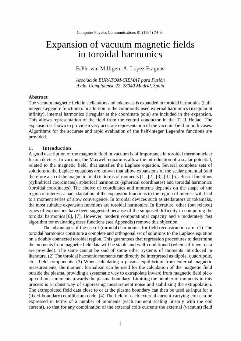
BR =sinhζ

Rp

1 − coshζ cos η( )sinhζ

∂ψ∂ζ

− sinη∂ψ∂η

, (10a)

BZ =sinhζ

Rp

−sinη∂ψ∂ζ

−1 − coshζ cosη( )

sinhζ∂ψ∂η

, (10b)

Bφ =coshζ − cosη( )

Rp sinhζ∂ψ∂φ

. (10c)

The contribution of the moment introduced in Eq. (7c) to the total field is found to be:

BR = δ intM00η coshζ − cosη sinη

4Rp sinhζcoshζP1/2

0 (coshζ ) − P− 1/20 (coshζ)[ ] , (10d)

Bz =− δ intM00η coshζ − cosη

4Rp

cosηP1/20 (coshζ) − P−1 / 2

0 (coshζ )[ ] , (10e)

Bφ = 0 . (10f)

Note that these expressions can also be written in cylinder coordinates in terms of the morefamiliar elliptic functions K and E [2].

For a magnetic field given on a number of grid points, the moments are determined by aregression using Eqs. (7) and (10) to find a linear expression of the field components in themoments, the latter being the regression coefficients.

3 . Application to stellarators

As test cases for the potential of the moment formalism as presented in the previous sections,two stellarators were analysed. TJ-IU, an l = 1 torsatron, and TJ-II, an l = 1 heliac with centralconductor, both under construction at the Asociación EURATOM-CIEMAT para Fusión. Thefields corresponding to these machines were computed on a number of Ngrid points forstandard configurations of coil currents, and the moments were determined by the regressionprocedure described in the previous section. The grid points were selected randomly within aspecified region, in order to improve the regression and avoid aliasing effects. Then the fieldwas reconstructed from the obtained moments, and the following two global error indicatorswere introduced:The average error <ε>:

< ε >=B rec − Borig 2∑( )/ Ngrid

Borig∑( )/ Ngrid

(11a)

and the maximum error εmax:

6

εmax = maxBrec − Borig

Borig

(11b)

Here Brec refers to the field as reconstructed using the expansion in toroidal harmonics, andBorig to the original field as calculated from the coil currents using Biot-Savart's Law. Thesummation in Eq. (11a) and the maximum in Eq. (11b) are taken over all grid points. Thesequantities are well-defined because in the configurations we studied the B-field did not vanishanywhere.

3.1 Expansion of a TJ-IU standard configuration without plasma

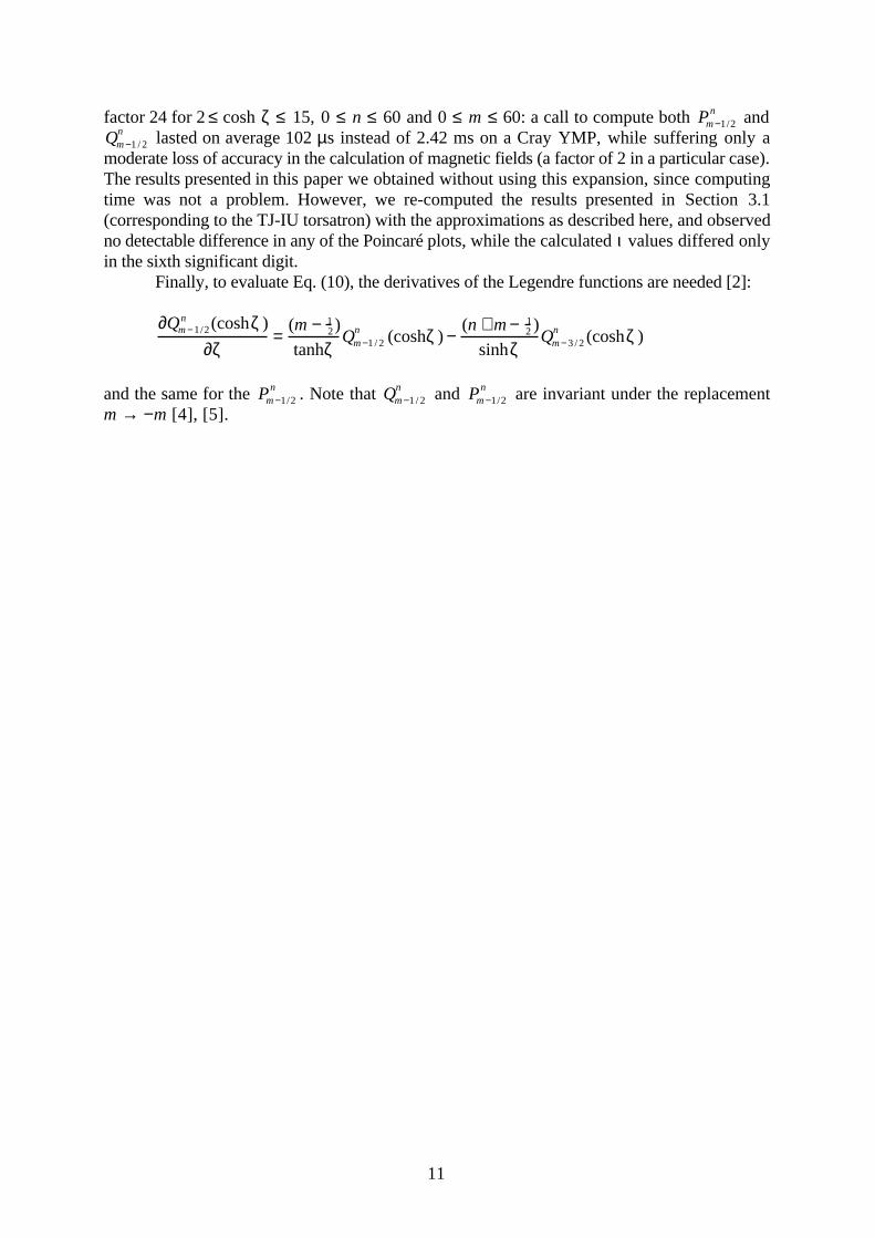
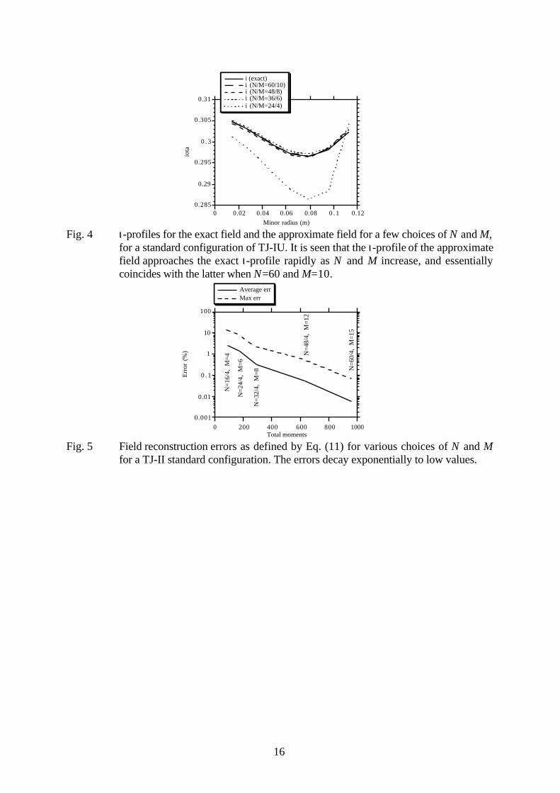
A standard TJ-IU Torsatron field configuration was analysed. TJ-IU has the followingparameters: l = 1, Toroidal periodicity NT = 6, major radius R0 = 0.6 m, minor radius of theregion of interest (the plasma region) amin = 0.15 m, inner minor radius of the helical coilacoil = 0.24 m. The pole of the toroidal coordinate system is chosen at Rp = 0.55 m, andcosh(ζ0) = 5. The stellarator symmetry is given by Eq. (8a) (s = −1). We considered a toroidalregion 0 ≤ r ≤ amin , 0 ≤ θ < 2π and 0 ≤ φ < 2π, and selected 500 points randomly in thisregion for which the field was calculated from given external coil currents. The momentsexpansion of the field was fitted to these data. In the expansion (7) only the termsn = 0, 6, 12, ..., N were used because of the toroidal periodicity of NT = 6. Because nocurrents flow in the internal region (no plasma), all internal moments were set to 0 (δint = 0).Fig. 2 shows the field reconstruction errors as defined by Eq. (6) for various choices of N andM for a standard configuration. It is observed that the errors decay exponentially to very lowvalues, and that the regression remains stable even at very large numbers of moments, due tothe orthogonality of the expansion functions. Fig. 3 shows Poincaré plots for the exactmagnetic field (as calculated from Biot-Savart's Law) and the approximate field as calculatedform the moments for a few choices of N and M. It is observed that the approximationimproves as N and M increase, and that for N = 60, M = 10 there is no visible difference withthe exact field, not only in the shape of the flux surfaces but even in the position of theindividual points forming the Poincaré plot. Finally, Fig. 4 shows the ι-profiles for the exactfield and the approximate field for a few choices of N and M. It is seen that the ι-profile of theapproximate field approaches the exact ι-profile rapidly as N and M increase, and essentiallycoincides with the latter when N = 60 and M = 10.

3.2 Expansion of a TJ-II standard configuration without plasma

The stellarator TJ-II is a heliac with a central conductor with l = 1 and toroidal periodicityNT = 4, major radius R0 = 1.5 m [9]. The stellarator symmetry is given by Eq. (8a) (s = −1).As mentioned in section 2, the topology of the 32 circular toroidal field (TF) coils (8 per period)does not permit, in theory, the definition of a region of validity as with TJ-IU, because of theirhelical swing. The TF coils are circular with a radius of 0.425 m, and the centreRc(φ), Zc(φ) of each coil is displaced by a distance rswing = 0.2825 m from the major axisR = R0, Z = 0, according to the law Rc = R+ rswing cos(NTφ) and Zc = −rswing sin(NTφ). Thefield generated by the TF coils is mainly toroidal, although some radial and vertical fields existin the interstitial coil regions (i.e. field ripple) which is mainly of importance near the coils andis small in the region of interest, well inside the TF coils. Therefore, modelling each TF coilwith one which has a larger radius at the same position (carrying a correspondingly larger

7

current in order to generate the same toroidal field) will not affect the field in the region ofinterest much; more specifically, this procedure does not affect the average toroidal field at all,but it neglects the field ripple. Thus, computing the moments assuming that the TF coils have asufficiently large radius such that they do not invade the region ζex < ζ < ζin (although in realitythey do) should be able to give a reasonable reproduction of the total magnetic field, exceptperhaps for the field ripple. We investigate this in the following.

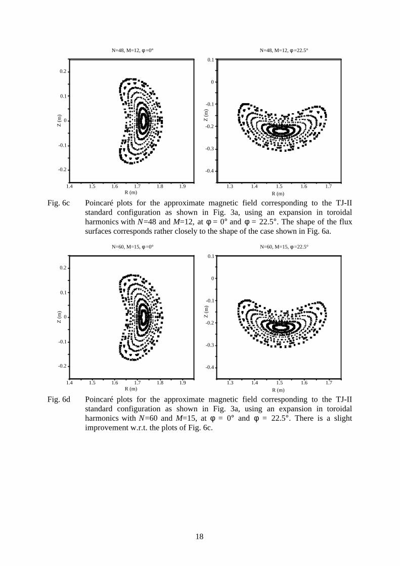
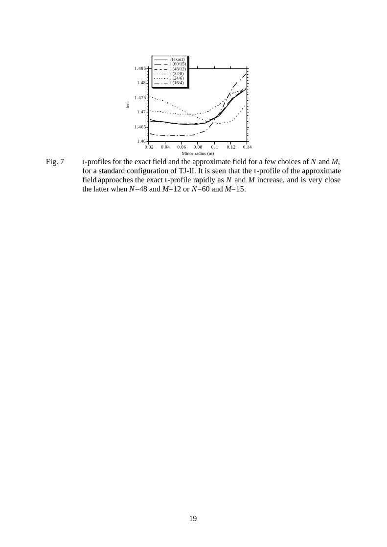
We considered a helical region that remained within the TF coils everywhere. In eachplane φ = constant, the boundary of the region is an ellipse with short half axis a = 0.175 m andlong half axis b = εa, where the ellipticity is ε = 1.4. The ellipse is centered on Re(φ), Ze(φ)with Re = R0+ reswingcos(NTφ) and Ze = −reswingsin(NTφ) where reswing = 0.18 m. The majoraxis b of the ellipse is perpendicular to the direction (Re − R0, Ze). Finally, points less than adistance 0.13 m from the major axis are excluded from the region. This elliptical-helical regionwith a gap is designed to approximately enclose a typical plasma. The pole of the toroidalcoordinate system is chosen at Rp = 1.5 m, and cosh(ζ0) = 5.7. We selected 1000 pointsrandomly in this region for which the field was calculated from given external coil currents. Themoments expansion of the field was fitted to these data. In the expansion (7) only the terms n =0, 4, 8, ..., N were used because of the toroidal periodicity of NT = 4. To represent the fieldgenerated by the central conductor, the internal moments were used (δint = 1). Fig. 5 displaysthe field reconstruction errors for various choices of N and M for a standard configuration.Again, it is observed that the errors decay exponentially to very low values and that theregression remains stable even at very large numbers of moments. Also, it is seen that theinclusion of moments with n = 32 leads to an additional reduction of the reconstruction error(over the exponential decay), because that allows representation of the field ripple (recall thatthere are 32 TF coils). Further it is seen that the presence of the TF coils in the region of validitydoes not affect the accuracy much, probably because of the reason given earlier: they may bereplaced by an equivalent set of coils not invading the region of validity but generatingessentially the same field in the helical region of interest as defined above. Fig. 6 showsPoincaré plots for the exact magnetic field (as calculated from Biot-Savart's Law) and theapproximate field as calculated form the moments for a few choices of N and M. It is observedthat the approximation improves as N and M increase, and that for N=48, M=12 there is onlysome slight difference with the exact field left. For N=60, M=15 the field errors as definedabove are reduced (see Fig. 5) but the Poincaré plot shows that, although the interior fluxsurfaces are reproduced with excellent precision, the outermost flux surface suffers some smallhigher-harmonic deformation, due to overfitting. Finally, Fig. 7 shows the ι-profiles for theexact field and the approximate field for a few choices of N and M. It is seen that the ι-profile ofthe approximate field approaches the exact ι-profile rapidly as N and M increase.

4 . Future extensions of this work

A first extension of the work presented here is to calculate the moments in the presence of aplasma from the field in the vacuum region surrounding the plasma. It is to be foreseen that thiswill cause no difficulties in the TJ-IU case, since the plasma can simply be represented by theinternal moments. In the case of TJ-II, however, due to the helical shape of the plasma and thepresence of the central conductors, this may be not so simple and probably only the part of thevacuum field on the outside of the plasma (i.e. on the side away from the central conductor) canbe represented by toroidal harmonics.

In the case of TJ-IU and perhaps also in the case of TJ-II we will then create a smalldatabase containing some scans of the most important plasma parameters and the response ofthe moments. This can be used to create a bigger database by interpolating between equilibria in

8

moments-space, which may then be used in statistical analyses to determine the response of(magnetic) diagnostics to plasma parameters (this will aid data interpretation). It is evenforeseen to use this bigger database to design the magnetic diagnostic in such a way that itprovides maximum information on some selected plasma parameters.

5 . Conclusions and comparison with other systems of moments

Expanding the vacuum magnetic field in stellarators (or tokamaks) in toroidal harmonics is asuccessful method for representing the field in a compact manner. The toroidal harmonics orhalf-integer Legendre functions form a complete and orthogonal set of expansion functions,which allows determination of the moments with very good precision that is only limited bycomputational accuracy. Other expansion functions have been suggested in literature for thisproblem, but all seem to suffer from some drawbacks compared to the system of momentsdiscussed here. The cylindrical expansion functions with a first-order toroidal correction assuggested in [7] are complete nor orthogonal, and consequently the reconstruction error <ε>does not drop to very low values (in [7], <ε> = 0.46 % is mentioned as best result for astandard ATF configuration without plasma, but it should be mentioned that only a very smallnumber of moments was used). The Dommaschk potentials [6], which are both orthogonal andcomplete for fields regular at the torus axis, have the advantage that they are easy to evaluate,but, as noted in [6], they fail to represent Heliac fields with singularities at the toroidal axis,because they do not contain the equivalent of the internal moments as described in this paper.We have demonstrated that the half-integer Legendre functions can even approximate vacuumHeliac fields with high accuracy (the TJ-II case).

It has been said many times that the half-integer legendre functions are difficult toevaluate (e.g. [6]). In the Appendix to this paper we provide an analysis of this supposeddifficulty and a solution. We do not believe that the numerical evaluation of the half-integerLegendre functions is an obstacle to their use.

AcknowledgementsThis work was made possible by Commission of the European Communities BursaryERB4001GT921485. The authors would like to thank the TJ-IU and TJ-II teams at theAsociación EURATOM-CIEMAT para Fusión for a very pleasant cooperation.

9

Appendix

A.1 Toroidal coordinates inverse transformation

The transformation from cylindrical coordinates (R, Z, φ) to toroidal coordinates (ζ, η, φ) (theinverse of Eq. (3)) is carried out as follows:

tanhζ = 2R

Rp

+Z 2

RRp

+Rp

R

− 1

, tanη =Z sinhζ

Rcoshζ − Rpsinhζ

A.2 Evaluation of the half-integer Legendre functions

In this Appendix, we discuss an algorithm to evaluate the half-integer Legendre functions ortoroidal harmonics, since there are no standard computer library routines available for thesefunctions. The half-integer Legendre functions can be expressed in terms of the Hypergeometricfunction F(a, b; c; z) = 2 F1a, b; c; z) [1, 2] (Note an unimportant difference of a factor (-1)n

between the Qm −1 / 2n 's and of a factor −1( )n

between the Pm −1/2n 's in the two cited references,

as discussed in [5]. We adopt the normalization of [2]):

Pm −1/2n (coshζ) =

Γ(m + n + 12 )

2n n!Γ(m − n + 12 )

tanhn ζ coshm −1 / 2 ζ

×F 12 n − m + 1

2( ), 12 n − m + 3

2( );n +1;tanh2 ζ[ ] (A.1)

Qm −1 / 2n (coshζ) =

Γ 12( )Γ(m + n + 1

2 )

2m+1 / 2 Γ(m + 1)

tanhn ζcoshm +1/2 ζ

×F 12 m + n + 1

2( ), 12 m + n + 3

2( );m +1;1

cosh2 ζ

(A.2)

where Γ(x) is the Gamma function.The Hypergeometric function F(a, b; c; z) can be expanded as a series (note that here a,

b, c, z are all real and 0 < z < 1) [2]:

F(a,b;c;z) = S(i)i =0

∞

∑ , with S(i) =(a + i − 1)(b + i −1)

(c + i −1)

z

iS(i −1), i ≥ 1, and S(0) = 1.

Convergence is discussed in [2]. If this series is truncated at some number i = itrunc,itrunc >> max(1, |a|, |b|, |c|), the absolute error ε in F(a, b; c; z) is estimated by

ε(itrunc ) = S(itrunc)z

1 − z .

Thus it is seen that truncation errors are important for Pm −1/2n (coshζ) when ζ is large (near the

pole of the coordinate system), and for Qm −1 / 2n (coshζ) when ζ is close to 0. The series is

evaluated (itrunc incremented) until ε rel(itrunc) falls below some preset relative precision δ:

10

ε rel(itrunc) = ε(itrunc) S(i)i = 0

itrunc

∑

−1

< δ

or when itrunc reaches some preset maximum N trunc. A best estimate for F(a, b; c; z) from thetruncated series, with the condition that itrunc >> max(1, |a|, |b|, |c|), is then given by:

F(a,b;c;z) ≈ S(i)i =0

itrunc

∑ + ε(itrunc )

(we only use this estimate when itrunc reaches N trunc).It turns out that for values of the argument in the range 2 ≤ cosh ζ ≤ 15 (this range

amply covers the requirements we have encountered in practice), the hypergeometric seriescorresponding to Qm −1 / 2

n converges rapidly (itrunc ≤ 73 for a wide range of n- and m-values, i.e.0 ≤ n ≤ 60 and 0 ≤ m ≤ 60, when the termination criterion is set to δ = 10−10), whereas theseries corresponding to Pm −1/2

n converges much slower (itrunc ≤ 5247 under the sameconditions). Note, however, that the convergence of the series corresponding to Pm −1/2

n

improves as m increases (itrunc ≤ 985 for m > 10 under the above conditions). Note, also, thatthese values of itrunc are maxima taken over the whole range of ζ-, n- and m-values as specified;in general the series converge much faster (e.g. itrunc is of the order of 10 in most cases forQm −1 / 2

n ). Finally, recall that the Pm −1/2n are only required when internal field sources are present

(cf. Eq. (7)).Evaluation of Qm −1 / 2

n and Pm −1/2n for a range of m-values for fixed n and ζ can be done

more efficiently using the recurrence relations [2]:

Pm −1/2n = (m − n + 1

2 )−1 2mcoshζPm −1/2n − (m + n − 1

2 )Pm −3/2n( ) , (A.3)

Qm −3 / 2n = (m + n − 1

2 )−1 2mcoshζQm − 1/2n − (m − n + 1

2 )Qm +1 / 2n( ) . (A.4)

These relations should be used in the manner as suggested by Eqs. (A.3) and (A.4), i.e. withascending m for Pm −1/2

n and descending m for Qm −1 / 2n , in order to retain the largest possible

number of significant digits in the results.Computation time may be further reduced by introducing the following approximation:

log Pm −1 / 2n (coshζ)( ) = α0

nm +α1nm log(coshζ) + α2

nm coshζcoshζnorm

+⋅ ⋅ ⋅+ αknm coshζ

coshζnorm

k −1

+⋅⋅⋅ , (A.5)

where the coefficients αknm are found from a least-squares fit to the Legendre functions as

calculated using the method described above, and are stored in a file for later use. The sametype of expansion is also used to find approximations to Qm −1 / 2

n (coshζ) . Note that theexpansion ignores the sign of Pm −1/2

n and Qm −1 / 2n . Pm −1/2

n is negative if and only if m < n andm + n = odd, while Qm −1 / 2

n is always positive. We found that for 2 ≤ cosh ζ ≤ 15, 0 ≤ n ≤ 60and 0 ≤ m ≤ 60, taking cosh ζnorm = 5.7 and truncating this expansion at k = 16, the averageand maximum relative errors in the calculation of Pm −1/2

n are ε relP (av) = 4 ×10−5 and

ε relP (max) = 1 × 10−3 , and similar numbers for Qm −1 / 2

n . The error in the series approximation ofPm −1/2

n and Qm −1 / 2n increases almost linearly with n. We achieved an average acceleration of a

11

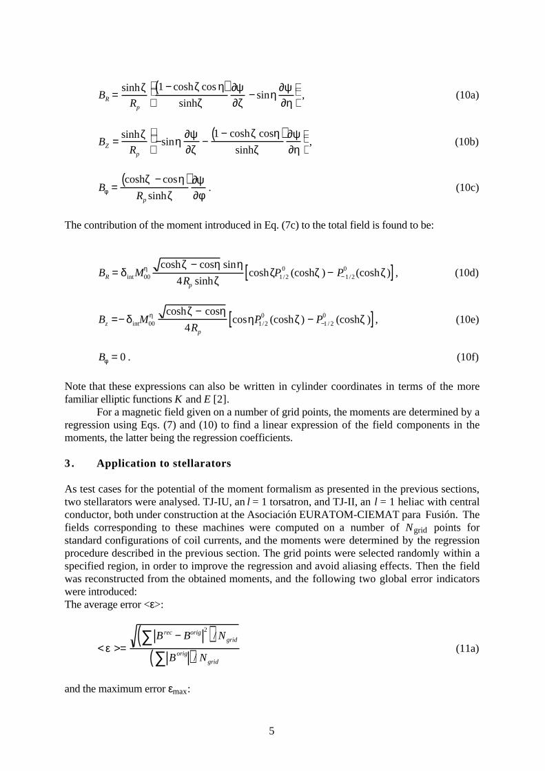
factor 24 for 2 ≤ cosh ζ ≤ 15, 0 ≤ n ≤ 60 and 0 ≤ m ≤ 60: a call to compute both Pm −1/2n and

Qm −1 / 2n lasted on average 102 µs instead of 2.42 ms on a Cray YMP, while suffering only a

moderate loss of accuracy in the calculation of magnetic fields (a factor of 2 in a particular case).The results presented in this paper we obtained without using this expansion, since computingtime was not a problem. However, we re-computed the results presented in Section 3.1(corresponding to the TJ-IU torsatron) with the approximations as described here, and observedno detectable difference in any of the Poincaré plots, while the calculated ι values differed onlyin the sixth significant digit.

Finally, to evaluate Eq. (10), the derivatives of the Legendre functions are needed [2]:

∂Qm − 1/2n (coshζ )

∂ζ=

(m − 12)

tanhζQm −1 / 2

n (coshζ ) −(n + m − 1

2 )

sinhζQm − 3 / 2

n (coshζ )

and the same for the Pm −1/2n . Note that Qm −1 / 2

n and Pm −1/2n are invariant under the replacement

m → −m [4], [5].

12

References

[1] Morse and Feshbach, Methods of theoretical physics, McGraw-Hill, New York, 1953[2] Abramowitz and Stegun, Handbook of mathematical functions, Dover, New York,

1972[3] K. Miyamoto, Recent stellarator research, Nucl. Fusion 18 (1978) 243 - 284[4] J.R. Cary, Construction of three-dimensional vacuum magnetic fields with dense nested

flux surfaces, Phys. Fluids 27 (1984) 119 - 128[5] B.J. Braams, Computational studies in tokamak equilibrium and transport, Thesis,

FOM-Institute "Rijnhuizen", Nieuwegein, The Netherlands (1986)[6] W. Dommaschk, Representations for vacuum potentials in stellarators, Comp. Phys.

Comm. 40 (1986) 203-218[7] G.H. Neilson, J.H. Harris, Harmonic analysis for magnetic configuration control in

experimental stellarator devices, Nucl. Fusion 27 (1987) 711-724[8] F. Alladio, F. Chrisanti, Analysis of MHD equilibria by toroidal multipolar expansions,

Nucl. Fusion 26 (1986) 1143[9] C. Alejaldre, J.J. Alonso Gonzalo, J. Botija Perez, et al., TJ-II project: a flexible heliac

stellarator, Fusion Techn. 17 (1990) 131-139

13

Figures

R

Z

ζ = ζ in ζ = ζ ex

Plasma

Region of validity External coils

Fig. 1 Region of validy of the expansion of the vacuum magnetic field in toroidalharmonics. The region is delimited by two coordinate surfaces such that ζex < ζ <ζin . Within this region the current density is identically zero. Exceptions to the latterstatement are discussed in the text.

0.0001

0.01

1

100

0 100 200 300 400 500

Average errMax err

Err

or (

%)

N=

12/6

, M

=2

Total moments

N=

24/6

, M

=4

N=

36/6

, M

=6

N=

48/8

, M

=8

N=

60/6

, M

=10

N=

72/6

, M

=12

N=

84/6

, M

=14

Fig. 2 Field reconstruction errors as defined by Eq. (11) for various choices of N and Mfor a TJ-IU standard configuration. The errors decay exponentially to very lowvalues.

14

0.2

0.1

0

-0.1

-0.20.4 0.5 0.6 0.7 0.8

R (m)

Z (

m)

Exact, φ =0°

0.2

0.1

0

-0.1

-0.20.4 0.5 0.6 0.7 0.8

R (m)

Z (

m)

Exact, φ =15°

Fig. 3a Poincaré plots for the exact magnetic field of a TJ-IU standard configuration (ascalculated from Biot-Savart's Law) at φ = 0° and φ = 15°. Note that the third andseventh surfaces (counting outwards) are close to the resonance ι = n/m = 6/20.

0.2

0.1

0

-0.1

-0.20.4 0.5 0.6 0.7 0.8

R (m)

Z (

m)

N=24, M=4, φ =0°

0.2

0.1

0

-0.1

-0.20.4 0.5 0.6 0.7 0.8

R (m)

Z (

m)

N=24, M=4, φ =15°

Fig. 3b Poincaré plots for the approximate magnetic field corresponding to the TJ-IUstandard configuration as shown in Fig. 3a, using an expansion in toroidalharmonics with N=24 and M=4, at φ = 0° and φ = 15°. Strong deformation of theflux surfaces w.r.t. Fig. 3a is observed.

15

0.2

0.1

0

-0.1

-0.20.4 0.5 0.6 0.7 0.8

R (m)

Z (

m)

N=48, M=8, φ =0°

0.2

0.1

0

-0.1

-0.20.4 0.5 0.6 0.7 0.8

R (m)

Z (

m)

N=48, M=8, φ =15°

Fig. 3c Poincaré plots for the approximate magnetic field corresponding to the TJ-IUstandard configuration as shown in Fig. 3a, using an expansion in toroidalharmonics with N=48 and M=8, at φ = 0° and φ = 15°. The shape of the fluxsurfaces corresponds closely to the shape of the case shown in Fig. 3a, but theindividual points in the plots do not correspond (indicating a significant differencein the ι-profile).

0.2

0.1

0

-0.1

-0.20.4 0.5 0.6 0.7 0.8

R (m)

Z (

m)

N=60, M=10, φ =0°

0.2

0.1

0

-0.1

-0.20.4 0.5 0.6 0.7 0.8

R (m)

Z (

m)

N=60, M=10, φ =15°

Fig. 3d Poincaré plots for the approximate magnetic field corresponding to the TJ-IUstandard configuration as shown in Fig. 3a, using an expansion in toroidalharmonics with N=60 and M=10, at φ = 0° and φ = 15°. No difference w.r.t. Fig.3a is detectable.

16

0.285

0.29

0.295

0 . 3

0.305

0.31

0 0.02 0.04 0.06 0.08 0 . 1 0.12

i (exact)i (N/M=60/10)i (N/M=48/8)i (N/M=36/6)i (N/M=24/4)

iota

Minor radius (m)

Fig. 4 ι-profiles for the exact field and the approximate field for a few choices of N and M,for a standard configuration of TJ-IU. It is seen that the ι-profile of the approximatefield approaches the exact ι-profile rapidly as N and M increase, and essentiallycoincides with the latter when N=60 and M=10.

0.001

0.01

0 . 1

1

10

100

0 200 400 600 800 1000

Average errMax err

Err

or (

%)

Total moments

N=

16/4

, M

=4

N=

24/4

, M

=6

N=

32/4

, M

=8

N=

48/4

, M

=12

N=

60/4

, M

=15

Fig. 5 Field reconstruction errors as defined by Eq. (11) for various choices of N and Mfor a TJ-II standard configuration. The errors decay exponentially to low values.

17

0.2

0.1

0

-0.1

-0.2

1.4 1.5 1.6 1.7 1.8R (m)

Z (

m)

1.9

Exact, φ =0° Exact, φ =22.5°

0

-0.1

-0.2

-0.3

-0.4

1.4 1.5 1.6 1.71.3

R (m)

Z (

m)

0.1

Fig. 6a Poincaré plots for the exact magnetic field of a TJ-II standard configuration (ascalculated from Biot-Savart's Law) at φ = 0° and φ = 22.5°. Note that the outermostsurface but one is close to the resonance ι = n/m = 28/19.

0.2

0.1

0

-0.1

-0.2

1.4 1.5 1.6 1.7 1.8R (m)

Z (

m)

1.9

N=24, M=6, φ =0° N=24, M=6, φ =22.5°

0

-0.1

-0.2

-0.3

-0.4

1.4 1.5 1.6 1.71.3

R (m)

Z (

m)

0.1

Fig. 6b Poincaré plots for the approximate magnetic field corresponding to the TJ-IIstandard configuration as shown in Fig. 3a, using an expansion in toroidalharmonics with N=24 and M=6, at φ = 0° and φ = 22.5°. Slight deformation of theflux surfaces w.r.t. Fig. 6a is observed, and the outermost surface but one is seennot to be close to resonance.

18

0.2

0.1

0

-0.1

-0.2

1.4 1.5 1.6 1.7 1.8R (m)

Z (

m)

1.9

N=48, M=12, φ =0° N=48, M=12, φ =22.5°

0

-0.1

-0.2

-0.3

-0.4

1.4 1.5 1.6 1.71.3

R (m)

Z (

m)

0.1

Fig. 6c Poincaré plots for the approximate magnetic field corresponding to the TJ-IIstandard configuration as shown in Fig. 3a, using an expansion in toroidalharmonics with N=48 and M=12, at φ = 0° and φ = 22.5°. The shape of the fluxsurfaces corresponds rather closely to the shape of the case shown in Fig. 6a.

0.2

0.1

0

-0.1

-0.2

1.4 1.5 1.6 1.7 1.8R (m)

Z (

m)

1.9

N=60, M=15, φ =0° N=60, M=15, φ =22.5°

0

-0.1

-0.2

-0.3

-0.4

1.4 1.5 1.6 1.71.3

R (m)

Z (

m)

0.1

Fig. 6d Poincaré plots for the approximate magnetic field corresponding to the TJ-IIstandard configuration as shown in Fig. 3a, using an expansion in toroidalharmonics with N=60 and M=15, at φ = 0° and φ = 22.5°. There is a slightimprovement w.r.t. the plots of Fig. 6c.

19

1.46

1.465

1.47

1.475

1.48

1.485

0.02 0.04 0.06 0.08 0 . 1 0.12 0.14

i (exact)i (60/15)i (48/12)i (32/8)i (24/6)i (16/4)

iota

Minor radius (m)

Fig. 7 ι-profiles for the exact field and the approximate field for a few choices of N and M,for a standard configuration of TJ-II. It is seen that the ι-profile of the approximatefield approaches the exact ι-profile rapidly as N and M increase, and is very closethe latter when N=48 and M=12 or N=60 and M=15.

20

Erratum

The following sentence (following Eq. (7c)):

The field thus generated is that of a line current I = 2πµ0( )−1M00

η eφ along the torus axis (pole)R = Rp, Z = 0.

should be replaced by:

The field thus generated is that of a line current I = 2 / µ0( )M00η eφ along the torus axis (pole)

R = Rp, Z = 0.