computer modeling for injection molding (simulation, optimization, and control) || learning control

13LEARNING CONTROL

Yi YangDeptartment of Control Science and Engineering, Zhejiang University, Hangzhou, Zhejiang, China

Furong GaoDepartment of Chemical and Biomolecular Engineering, Hong Kong University of Science and Technology, Kowloon, HongKong, China

As mentioned in Chapter 2, injection molding is a batchprocess with a repetitive nature, information of past controlsmay be explored for improvement of the current and futurecycles. This kind of cycle-to-cycle improvement is similarto that of the human learning process, therefore referred toas learning control .

13.1 LEARNING CONTROL

Generally, there are two ways to improve the learningcontrol performance along cycle direction, one is controllerparameter learning and the other is control signal learningcontrol.

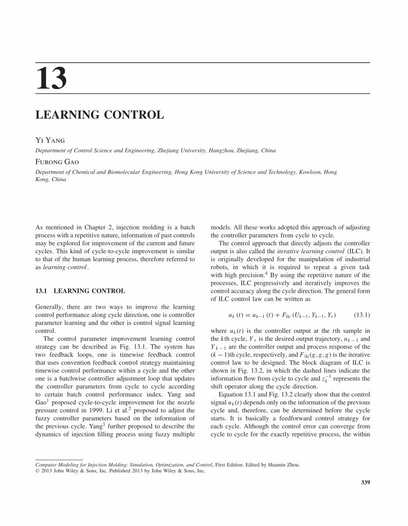
The control parameter improvement learning controlstrategy can be described as Fig. 13.1. The system hastwo feedback loops, one is timewise feedback controlthat uses convention feedback control strategy maintainingtimewise control performance within a cycle and the otherone is a batchwise controller adjustment loop that updatesthe controller parameters from cycle to cycle accordingto certain batch control performance index. Yang andGao1 proposed cycle-to-cycle improvement for the nozzlepressure control in 1999. Li et al.2 proposed to adjust thefuzzy controller parameters based on the information ofthe previous cycle. Yang3 further proposed to describe thedynamics of injection filling process using fuzzy multiple

Computer Modeling for Injection Molding: Simulation, Optimization, and Control, First Edition. Edited by Huamin Zhou.© 2013 John Wiley & Sons, Inc. Published 2013 by John Wiley & Sons, Inc.

models. All these works adopted this approach of adjustingthe controller parameters from cycle to cycle.

The control approach that directly adjusts the controlleroutput is also called the iterative learning control (ILC). Itis originally developed for the manipulation of industrialrobots, in which it is required to repeat a given taskwith high precision.4 By using the repetitive nature of theprocesses, ILC progressively and iteratively improves thecontrol accuracy along the cycle direction. The general formof ILC control law can be written as

uk (t) = uk−1 (t) + Filc (Uk−1, Yk−1, Yr) (13.1)

where uk (t) is the controller output at the t th sample inthe k th cycle, Y r is the desired output trajectory, uk − 1 andY k − 1 are the controller output and process response of the(k − 1)th cycle, respectively, and F ilc(g , g , g) is the iterativecontrol law to be designed. The block diagram of ILC isshown in Fig. 13.2, in which the dashed lines indicate theinformation flow from cycle to cycle and z−1

k represents theshift operator along the cycle direction.

Equation 13.1 and Fig. 13.2 clearly show that the controlsignal uk (t) depends only on the information of the previouscycle and, therefore, can be determined before the cyclestarts. It is basically a feedforward control strategy foreach cycle. Although the control error can converge fromcycle to cycle for the exactly repetitive process, the within

339

340 LEARNING CONTROL

FIGURE 13.1 Block diagram of parameter learning controlsystem.

FIGURE 13.2 Generalized iterative learning control system.

cycle disturbances cannot be rejected. It is necessary tocombine the ILC law Equation 13.1 with the real timefeedback controller to form a feedback feedforward ILC,as formulated below,

uk (t) = ufb,k (t) + uilc,k (t) (13.2)

ufb,k (t) = Ffb

(Yr, Uk

(∣∣∣∣ 0t − 1

), Yk

(∣∣∣∣0t))

(13.3)

uilc,k (t) = uilc,k−1 (t) + Filc (Yr , Uk−1, Yk−1) (13.4)

where u ilc, k (t) and u fb, k (t) are the iterative learning actionand feedback control action of the t th sample in the

k th cycle, respectively. Uk

(∣∣∣∣ 0t − 1

)and Yk

(∣∣∣∣0t)

are the

historical controller output and input series up to the t thsample of the k th cycle, respectively. The block diagramof control system described by Equations 13.2–13.4 canbe seen from Fig. 13.3. There are two feedback loops inthis system, one is the real-time feedback along the timeaxis within a cycle and the other is the feedback along thecycle direction to ensure a cyclewise convergence satisfyingcertain criterion.

uilc’k−1(t)

uilc’k(t)

ufb’k(t)

Yr

FIGURE 13.3 Feedback feedforward ILC system.

The feedback plus feedforward ILC is the main stream ofthe research on learning control area, detailed reviews canbe found in References 5 and 6. The key problem is to selecta proper model and algorithm to determine F ilc(g , g , g) andF fb(g , g , g). In 1999, Havlicsek and Alleyne7 proposed afeedback ILC combined control for injection ram velocity.In 2002, Tan and Tang8 proposed a cycle-to-cycle learningfor injection filling phase based on the linear feedbackcontrol to deal with the nonlinear uncertain dynamics. In2004, Ouyang et al.9 designed a control system in which atimewise proportional-derivative (PD) controller combinedwith a neural-network-based cyclewise ILC controller forinjection velocity control. In 2008, Yao et al.10 adoptedthe feedback feedforward ILC for the barrel temperaturecontrol and reduced the steady-state temperature to a rangewithin ±0.3 ◦C. This kind of control was also adopted forthe V/P switchover point detection.11

Learning control strategy is proposed to exploit therepetitive nature of injection molding process like anyother batch processes. The advantage of learning controlis that the control can converge well along the cycledirection when the process dynamics is exactly repeatable.Furthermore, the design of control law F ilc(g , g , g) requireslittle process knowledge, with relatively good robustness.The major problem of the learning control is that when thereare uncertain disturbances and nonrepetitive dynamics,there are no guidelines on how to design and balanceF ilc(g , g , g) and F fb(g , g , g).

13.1.1 Learning Control for Injection VelocityProfiling

Filling is the first phase of the injection molding process.The injection velocity has an important influence on the

LEARNING CONTROL 341

Ab Vm

Amf

IV

Barrel

Mold cavity

FIGURE 13.4 Illustration of the mold filling.

flow pattern inside the mold cavity, hence determinesthe evenness of the molded products.12,13 Although theinjection velocity can be accurately closed-loop controlledwith good robustness with the methods of Chapter 12, thesetting of the velocity profile remains as a difficult task.For a given mold and material, how the injection velocityshould be profiled to produce a part with evenly distributedquality? Before going further, it must be clarified that theinjection velocity is the velocity of the screw motion, whichis different from the melt-front velocity inside the mold.A schematic illustration of the mold filling is shown inFig. 13.4, in which IV is the screw injection velocity, V m

the melt-front velocity in the mold, Ab the cross-sectionalarea of the barrel, and Amf the corresponding melt-front areainside the mold. It is clear that the melt-front velocity isinfluenced by the mold geometry. Researchers in injectionmolding area14 have all recommended that a constant melt-front velocity during mold cavity filling should be used toprofile injection velocity, to minimize nonuniformity withinthe molded part. This, however, cannot be implementedbecause of the lack of a practical melt-front flow ratemeasurement method.

Recently, a transducer has been developed to measuremelt-front position (MFP) during mold filling by Gao andChen. The sensor output is linear to the melt-flow frontposition within the mold. Melt-front velocity is, simply, thederivative of the MFP. With such a transducer, the constantmelt-front velocity strategy can be translated to control theMFP to follow a constant ramp profile, as illustrated inFig. 13.5, in which a cascade control is adopted, consistingof two control loops. The inner loop is the injection velocitycontrol developed in Chapter 12; the outer control loopdetermines the injection velocity set point for the inner

FIGURE 13.5 Block diagram of the cascade melt-front velocitycontrol system.

velocity controller. The ramp rate is the melt-front velocity.Many existing control designs may be used for the outerloop controller, but they all require the development of adynamic model relating injection velocity to MFP. Effortof establishing such a model based on the fundamentalprinciples is tremendous, where the mold geometry factorsand the complicated flow and material properties have tobe involved. The development of such a model based onthe identification is inappropriate either, as this identifiedmodel will be mold dependent.

In view of the cyclic nature of the process, a model-freeILC method as introduced above is explored here to controlthe MFP without having to develop a detailed processmodel. The ILC, which is simple in control formulation,has found many applications for cases where detailedprocess knowledge is unavailable. In such a control system,information of last cycle is used to improve the control ofthe current cycle. The controller can be removed after anumber of cycles when a proper consistent profile has beenobtained for the inner velocity control loop.

13.1.1.1 ILC Formulation The ILC approach is adoptedhere to find a proper injection velocity profile to ensure thefilling of mold cavity at a uniform melt-front velocity.

Among many types of learning control laws proposed,a P-type learning control law is possibly the simplest, asformulated below,

uk+1 (t) = uk (t) + LPek (t) (13.5)

where u(t) is the process input at time t , e = y s − ym isthe error between the set point and real-time measurement,subscripts k and k + 1 denote the cycle number, and LP isthe ILC gain. It is clear that the control of the current cycleis based on the process input and the error of the last cyclein a point-to-point manner. Up to now, most of the ILCresults are for the systems without time delay. However, formany batch processes such as injection molding, the effectsof time delay cannot be ignored. There is a large delaybetween the injection velocity and the melt-front velocityresponse. During injection, there exists some melt betweenthe injection screw and the melt-flow front, and the meltis compressible coupled with its complicated viscoelasticproperties. Changes in the injection velocity cannot affectthe melt-front flow rate instantaneously. The long processdelay as well as variations of delay during filling makesit difficult to apply the simple point-to-point ILC method.To solve this problem, control law Equation 13.5 can bemodified to taken into consideration of the delay term:

uk+1 (t) = uk (t) + LPek (t + td) (13.6)

where td is an estimated delay time. In this equation, thecontrol error at time t + td is used to update the control


input at time t for the next cycle. Control law of Equation13.6 can be applied to cases for which the time delay isexactly known. For processes with an uncertain delay, thereis no guarantee that this control law will be convergent.

For a system with a varying delay bounded by h , Parket al.15 proposed to hold the control input at a constantover the duration h , resulting in a modified learning controllaw as

uk+1 (t) = uk (mh) + �ek (mh + dh + ξ,∀t ∈)

[mh,mh + h) ,m ∈ {0, 1, . . . ,M − d} (13.7)

where ek (mh + dh + ξ ) = yd(mh + dh + ξ ) − yk (mh + dh+ ξ ), ξ is the initial remainder, and dh + ξ is the upperlimit of the delay. The system divides the process timespan by the size of the time delay uncertainty h . It hasbeen shown that the convergence can be maintainedby this method.15 This idea is adopted by this work.Several modifications have to be made as detailed below,considering practical issues of the process.

13.1.1.2 Division of Injection Velocity Profile The firstmodification is on the division of the filling phase timespan. For a given mold, a given amount of melt needs tobe injected. Changes in the injection velocity profile bythe ILC makes the total filling time span to vary fromcycle to cycle. This creates difficulties for the division ofthe filling time span. Furthermore, time delay is a strongfunction of injection velocity, a slower injection velocityresults in a larger time delay. The amount of materialinjected into a mold can be reasonably well representedby the distance that the screw has traveled during injection,known as injection stroke. The injection stroke is, therefore,used to replace the time for the ILC implementation. Withthis change, the time delay has also been transformed intostroke delay. As described in Section 13.1.1.5, the use ofstroke to replace time for the ILC implementation can resultin a more consistent delay for the injection phase.

13.1.1.3 Change in Controlled Variable This chapteruses the slope of the MFP instead of MFP itself, as thecontrolled variable. Even though the derivative of MFP cangive melt-front velocity, it also results in a low signal-to-noise ratio. Thus, the velocity is obtained by linear curvefitting of MFP measurements as the following equation:

Dm = Vmdt + Dm0 (13.8)

where Dm is the MFP, V m is the slope of Dm, that is, themelt-front velocity.

Injection time

Inje

ctio

n ve

loci

ty s

et p

oint

FIGURE 13.6 A typical ramp set point profile of injectionvelocity.

13.1.1.4 Change in Manipulated Variable For mostmolding machines, the velocity profile can only be set in apiecewise form as illustrated in Fig. 13.6. It is desirableto use ramp profiles instead of step change profiles, asthe step change injection velocity causes abrupt changes inMFP response, which is not desirable. It has, therefore, beendecided to use the velocity ramp slope as the manipulatedvariable for the outer loop.

Considering all the above practical issues with injectionmolding, the ILC control for searching optimal injectionvelocity profile can be reformulated as

Rk+1 (n) = Rk (n) + LPek (n + nd) (13.9)

where Rk (n) is the velocity slope at nth stroke stepof the k th iteration, nd the stroke delay, e(n + nd) =V s(n + nd) − V m(n + nd), and other symbols are the sameas Equation 13.9. Figure 13.7 shows the profile searchingoverall scheme via ILC approach. The slopes of injectionvelocity settings are obtained by control law Equation 13.9,before they are reconstructed as the real injection velocityset point for the inner-loop control.

13.1.1.5 Experimental Results and Discussion All theexperiments were conducted using the high densitypolyethylene (HDPE) processed with the barrel tempera-ture of 200 ◦C, on the same injection molding machineas introduced above. Three mold inserts with significantchanges in geometry were used to test the system experi-mentally, as illustrated in Fig. 13.8. The sampling periodfor the inner-loop velocity control is 5 ms.

The first experiment is conducted with a constantinjection velocity of 25 mm/s. The responses of MFPmeasurements for the three different molds of Fig. 13.9 areshown in Fig. 13.10. It is clear that with a constant injectionvelocity, melt-front velocity varies with the changes inmold geometry. This indicates the necessity of profiling the

LEARNING CONTROL 343

FIGURE 13.7 Flow chart of profile searching by ILC.

injection velocity. The minor oscillations of MFP responsein Fig. 13.10 are due to the noises of the capacitancemeasurement.

The second experiment is conducted with mold 3 todemonstrate the delay variation, as shown in Fig. 13.11.Three MFP responses are obtained: one with a constantinjection velocity of 25 mm/s (dotted line), one with a stepchange injection velocity profile of 25–15 mm/s with thestep change introduced at 1000 ms injection time (solidline), and one with the same step change profile butdifferent step time of 1275 ms (dashed line). Take the MFPresponse of constant injection velocity as the reference, thepoint at which the MFP measurement begins to diverse fromthe reference line can be considered to be the starting timeof step change response, and the time difference betweenstep change time and the starting response time is the timedelay. It can be seen from Fig. 13.11 that the late stepchange obviously has much larger delay value than the earlystep change. The time delay changes not only with the melt-flow development but also with the injection velocity. Thesame measurements are plotted using the injection strokeas the x -axis, as shown in Fig. 13.12: Fig. 13.12a for earlystep change and Fig. 13.12b for late step change. The delayvariation in stroke shown in Fig. 13.12 is obviously muchsmaller than the delay in time of Fig. 13.11, indicating theadvantage of using the stroke.

0

0.0

0.2

0.4

MFP

out

put (

V)

Inje

ctio

n ve

loci

ty s

ettin

g (m

m/s

)

0.6

0.8

Constant velocity

Set pointThird iterationSecond iterationFirst iteration

Constant velocity

Third iterationSecond iterationFirst iteration

1.0

50 100 200

Injection time (*/5 ms)

300 350150 250

014

16

18

20

22

24

26

28

30

32

50 100 200

Injection time (*/5 ms)

300 350 400150 250

(a)

(b)

FIGURE 13.8 Simulation test of proposed ILC search methodon mold 3: (a) MFP responses and (b) corresponding velocitysettings.

The first step in the ILC controller design is to determinethe number of steps for the filling phase. Previous workssuggests that five steps of velocity profile are sufficientto achieve a satisfactory constant melt-front velocity.16

Considering the fact that most injection molding machineprovide 10 points injection velocity setting, that is, ninesteps of velocity profile, so it has been decided to use ninesteps for the velocity profiling in this section. The secondissue is to determine the learning gain LP. On the basis ofthe simulation results, LP has been determined to be 35 forthe experimental test. The set point for MFP slope, V s, isselected to be 1.0 in Equation 13.9. The stroke delay term,nd, is determined to be one step by the above open-looptest results.

To illustrate the problem with the straightforwardapplication of the point-to-point ILC of Equation 13.6,


(a) (b)

(c)

FIGURE 13.9 Geometry of molds: (a) mold insert 1, (b) mold insert 2, and (c) mold insert 3.

03.6

3.8

4.0

4.2

4.4

4.6

4.8

MFP

out

put (

V)

100

Mold 1Mold 2Mold 3

200 300Injection time (*5 ms)

400

FIGURE 13.10 MFP open-loop test using three molds.

experiment is conducted with the injection velocity settingsdirectly adjusted by the error between the MFP set point andmeasurement. The resulted melt-front position responsesare shown in Fig. 13.13, with the corresponding velocitysettings shown in Fig. 13.13b. It is clear that the MFP is farfrom a straight line even after 30 learning cycles, indicatingthat the point-to-point direct learning method cannot workwell. No significant improvement can be made with changesin learning rates.

The proposed search method as ILC control lawEquation 13.9 is thus tested on mold insert 2. The injectionstroke for filling this mold is 37.5 mm. This stroke isdivided into nine steps as [16.50, 18.83, 21.17, 23.50,25.83, 28.17, 30.50, 32.83, 35.17, 37.50], where 16.50 is thestarting point at which the melt front reaches the transducer.Figure 13.14a shows some MPF measurements for the firstiterations of learning. The initial injection velocity is set to

FIGURE 13.11 Illustration of the time delay variation.

be a constant of 25 mm/s. The corresponding MFP response,as indicated by the dashed line, accelerates because of thecontinuously decreasing cross-sectional area of the mold.After only two iterations, the third cycles MFP response,shown by the black solid line, overlaps well with the setpoint (gray solid line). The corresponding injection velocityprofiles are shown in Fig. 13.14b. Clearly, a decreasingvelocity profile, as shown in the solid line of Fig. 13.3b,can deliver a uniform filling of mold insert 2.

The mold insert 3 with stronger changes in the moldshape is used to test further the designed profile searchingscheme. The injection stroke is also divided into nine stepsof [16.5, 19.0, 21.5, 24.0, 26.5, 29.0, 31.5, 34.0, 36.5,39.0], because of the mold change. The ILC search scheme

TWO-DIMENSIONAL (2D) CONTROL 345

(a)

(b)

FIGURE 13.12 Illustration of delay in terms of stroke: (a) earlystep change and (b) later step change.

is applied to this new mold without any other changes.Again, the initial injection velocity is set to be a constant25 mm/s. The MFP responses are plotted in Fig. 13.3a. It isclearly shown that after three iterations, the MFP responseis very close a straight line. The corresponding velocityprofiles are shown in Fig. 13.15b. Owing to the delay, thevelocity setting after 350th samples has no effect on theMPF response, and it was thus set to be constant as shownin Fig. 13.15b.

13.2 TWO-DIMENSIONAL (2D) CONTROL

The feedback feedforward ILC shown in Fig. 13.3 isactually a 2D feedback control system, with one dimensionalong the cycle axis and the other dimension along thetime axis. From the viewpoint of a 2D system, the

(a)

150

3.6

3.8

4.0

4.2

4.4

4.6

4.8

250200 300

Injection time (∗5 ms)

MFP

out

put (

V)

350 450

Set pointCycle 30Cycle 20Cycle 10

Cycle 20Cycle 10

Cycle 2Cycle 1

Cycle 30Cycle 2Cycle 1

400

1500

10

15

25

30

40

35

45

20

5

250200 300


Inje

ctio

n ve

loci

ty s

ettin

g (m

m/s

)

350 450400

(b)

FIGURE 13.13 Point-to-point direct iterative searching ofthe injection velocity setting: (a) MFP responses and (b)corresponding velocity settings.

conventional ILC as shown in Fig. 13.2 is only a cyclewisefeedback control with cyclewise integral action ensuringthe performance improvement along the cycle direction.To guarantee the performance improvement along boththe time and cycle directions, 2D feedback controller isnecessary. The feedback feedforward ILC introduced earlieris actually a 2D feedback controller but without uniformand balanced design, analysis, and optimization in twodirections.

For batch processes such as injection molding, a moregeneral form of 2D feedback control system can be shownin Equation 13.11, where F 2D(·) denotes the 2D control lawto be designed. z−1

t and z−1k are the shift operator along the

time and cycle axes, respectively. The integral action alongthese two directions formed a 2D integrator cascaded for


(a)

(b)



FIGURE 13.14 Experimental test of the proposed ILC searchingmethod on mold insert 2: (a) MFP responses and (b) correspondingvelocity settings.

eliminating the control error within and along cycles. The2D control law F 2D(·) can be written as follows:

uk (t) = uk (t − 1) + vk (t) (13.10)

vk (t) = vk−1 (t) + F2D (Yr , Uk−1, Yk−1, Uk(∣∣∣∣ 0t − 1

), Yk

(∣∣∣∣0t))

(13.11)

The research work applying the 2D control to theinjection molding process is mainly done by Gao’s researchgroup in the Hong Kong University of Science andTechnology. The related works include the ILC basedon the 2D state feedback and output feedback robustdesign,17–19 2D robust fault-tolerant control for injectionmolding process,20 2D linear quadratic optimal control forinjection molding process,21,22 single-cycle-generalized andmulticycle-generalized two-dimensional model predictiveiterative learning control (2D MPILC) for injection moldingprocess,23–25 and higher-order generalized 2D model

(a)

(b)

Injection time (*5 ms)

Injection time (*5 ms)

FIGURE 13.15 Experimental test of the proposed ILC searchingmethod on mold insert 3: (a) MFP responses and (b) correspondingvelocity settings.

predictive iterative learning control schemes for injectionmolding process.26 Although the proposed control strategieswere applied to the injection velocity control in all theseworks, they can be extended for key parameters of otherbatch processes without much effort. References 27 and 28used similar 2D control algorithm for packing pressure andmold filling melt-front velocity control, both achieved goodcontrol performances. A multiphase 2D model predictiveiterative learning control schemes was later proposed byWang et al.29 for the filling and packing phases of injectionmolding, using similar design principle.

13.2.1 2D Control of Packing Pressure

13.2.1.1 Two-Dimensional Model Predictive IterativeLearning Control (2D MPILC) Algorithm The basic de-sign principle of 2D MPILC is introduced briefly here. The


detailed derivation and analysis were given in References23 and 25. An single-input-single-output (SISO) batch pro-cess can be described by the following controlled autore-gressive integrated moving average (CARIMA) model

�P : A(q−1

t

)yk (t) = B

(q−1

t

)�t (uk (t)) + wk (t) ;

t = 0, 1, . . . , T ; k = 1, 2, . . . (13.12)

where t and k represent the discrete time and cycle/batchindex, respectively; T is the time duration of each cycle;uk (t), yk (t), and wk(t) are the input, output, and disturbanceof the process at time t in the k th cycle, respectively; q−1

t

indicate the timewise unit backward shift operator; bothA

(q−1

t

)and B

(q−1

t

)are operator polynomials

A(q−1

t

) = 1 + a1q−1t + a2q

−2t + · · · + anq

−nt (13.13)

B(q−1

t

) = b1q−1t + b2q

−2t + · · · + bmq−m

t (13.14)

and �t represents the timewise backward differenceoperator, that is, �t (f (t , k )) = f (t , k ) − f (t − 1, k ).

For the above repetitive process, introduce an ILC lawwith the form

�ILC : uk (t) = uk−1 (t) + uk (t − 1) − uk−1 (t − 1) + rk (t) ;

u0 (t) = 0, t = −1, 0, 1, . . . , T (13.15)

where rk (t) is referred as the updating law to be determinedonline based on the MPC philosophy and u0(t) the initialprofile of iteration. Let q−1

k represents the cyclewise unitbackward shift operator, the uk (t) and rk (t) have thefollowing relationship,

uk (t) = 1(1 − q−1

k

) 1(1 − q−1

t

) rk (t) (13.16)

which is a 2D system with 2D integral transformation.Control law Equation 13.16 can be expressed equiva-

lently as

�t (uk (t)) = �t (uk−1 (t)) + rk (t) (13.17)

or�k (uk (t)) = �k (uk (t − 1)) + rk (t) (13.18)

where �k represents the cyclewise backward differenceoperator, that is, �k (f (t , k )) = f (t , k ) − f (t , k − 1).

Substituting Equation 13.18 into model Equation 13.12leads to the following 2D system:

�2D−P : A(q−1

t

)yk (t) = A

(q−1

t

)yk−1 (t) + B

(q−1

t

)rk (t)

+�k (wk (t)) (13.19)

where rk (t), yk (t), and �k (wk (t)) represent the input,output, and disturbance of the system, respectively.

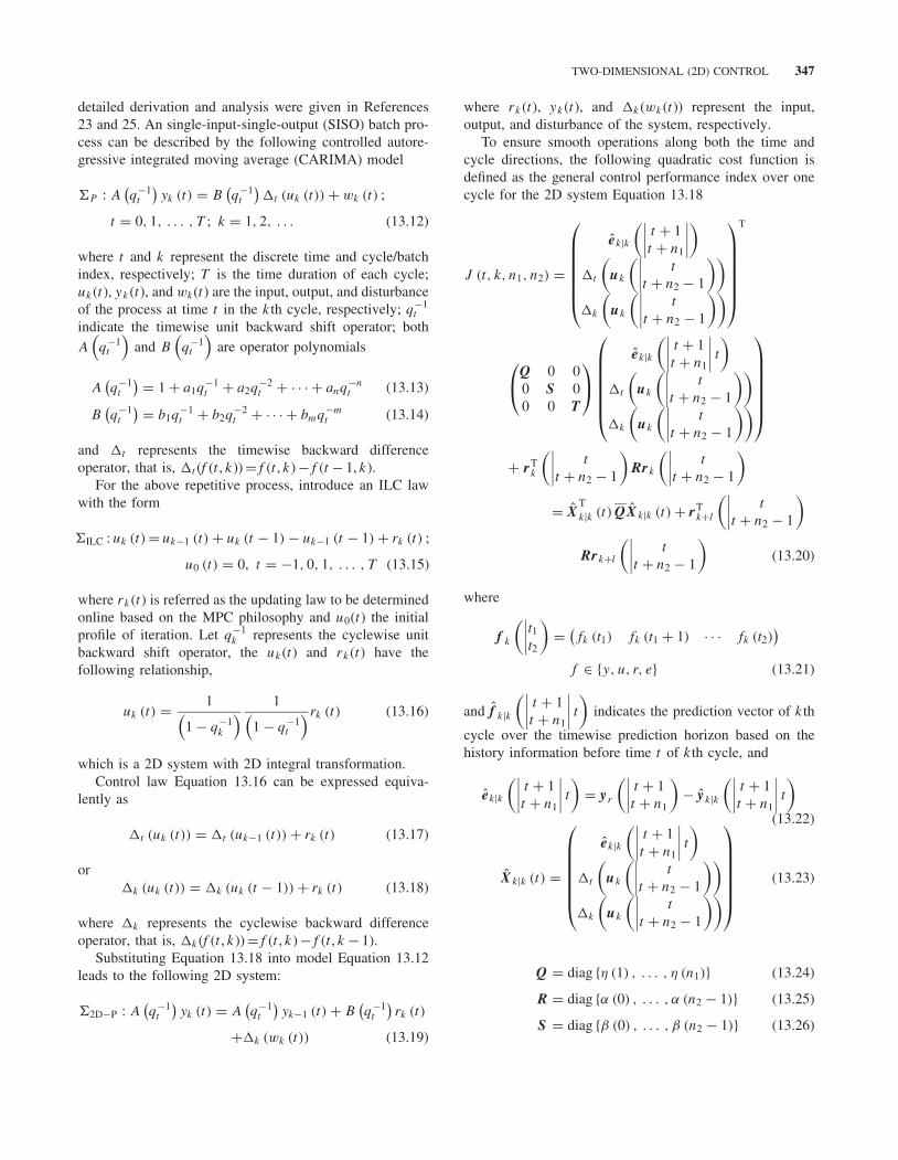
To ensure smooth operations along both the time andcycle directions, the following quadratic cost function isdefined as the general control performance index over onecycle for the 2D system Equation 13.18

J (t, k, n1, n2) =

⎛⎜⎜⎜⎜⎜⎜⎝

ek|k(∣∣∣∣ t + 1

t + n1

∣∣∣∣)

�t

(uk

(∣∣∣∣ t

t + n2 − 1

))

�k

(uk

(∣∣∣∣ t

t + n2 − 1

))

⎞⎟⎟⎟⎟⎟⎟⎠

T

⎛⎝Q 0 0

0 S 00 0 T

⎞⎠

⎛⎜⎜⎜⎜⎜⎜⎝

ek|k(∣∣∣∣ t + 1

t + n1

∣∣∣∣ t)

�t

(uk

(∣∣∣∣ t

t + n2 − 1

))

�k

(uk

(∣∣∣∣ t

t + n2 − 1

))

⎞⎟⎟⎟⎟⎟⎟⎠

+ rTk

(∣∣∣∣ t

t + n2 − 1

)Rrk

(∣∣∣∣ t

t + n2 − 1

)

= XTk|k (t) QX k|k (t) + rT

k+l

(∣∣∣∣ t

t + n2 − 1

)

Rrk+l

(∣∣∣∣ t

t + n2 − 1

)(13.20)

where

f k

(∣∣∣∣t1t2)

= (fk (t1) fk (t1 + 1) · · · fk (t2)

)

f ∈ {y, u, r, e} (13.21)

and f k|k

(∣∣∣∣ t + 1t + n1

∣∣∣∣ t)

indicates the prediction vector of k th

cycle over the timewise prediction horizon based on thehistory information before time t of k th cycle, and

ek|k(∣∣∣∣ t + 1

t + n1

∣∣∣∣ t)

= y r

(∣∣∣∣ t + 1t + n1

)− yk|k

(∣∣∣∣ t + 1t + n1

∣∣∣∣ t)

(13.22)

X k|k (t) =

⎛⎜⎜⎜⎜⎜⎜⎝

ek|k(∣∣∣∣ t + 1

t + n1

∣∣∣∣ t)

�t

(uk

(∣∣∣∣ t

t + n2 − 1

))

�k

(uk

(∣∣∣∣ t

t + n2 − 1

))

⎞⎟⎟⎟⎟⎟⎟⎠

(13.23)

Q = diag {η (1) , . . . , η (n1)} (13.24)

R = diag {α (0) , . . . , α (n2 − 1)} (13.25)

S = diag {β (0) , . . . , β (n2 − 1)} (13.26)


T = diag {γ (0) , . . . , γ (n2 − 1)} (13.27)

Q = diag {Q, S , T } (13.28)

By the procedure proposed in References 23 and 25 thebest prediction model for the 2D system, Equation 13.19can be formulated as follows:

yk|k

(∣∣∣∣ t + 1t + n1

∣∣∣∣ t)

= Grk

(∣∣∣∣ t

t + n2 − 1

)+ yk−1

(∣∣∣∣ t + 1t + n1

)

+ F k (t) (13.29)

the detailed formulation of matrix G and Fk (t) can befound in References 23 and 25.

To minimize cost function Equation 13.20, the followingrelationships between variables

�t

(uk

(∣∣∣∣ t

t + n2 − 1

))and �k

(uk

(∣∣∣∣ t

t + n2 − 1

))

and updating variable

rk

(∣∣∣∣ t

t + n2 − 1

)

are required

�t

(uk

(∣∣∣∣ t

t + n2 − 1

))= rk

(∣∣∣∣ t

t + n2 − 1

)

+�t

(uk−1

(∣∣∣∣ t

t + n2 − 1

))(13.30)

rk

(∣∣∣∣ t

t + n2 − 1

)= H �k

(uk

(∣∣∣∣ t

t + n2 − 1

))

−�k (uk (t − 1)) |n2 (13.31)

where

H =

⎛⎜⎜⎜⎜⎜⎝

1 0 0 · · · 0−1 1 0 · · · 00 −1 1 · · · 0...

......

. . ....

0 0 0 · · · 1

⎞⎟⎟⎟⎟⎟⎠

n2×n2

,

�k (uk (t − 1)) |n2 =

⎛⎜⎜⎜⎜⎜⎝

�k (uk (t − 1))

00...

0

⎞⎟⎟⎟⎟⎟⎠

n2×1

(13.32)

Let V = H − 1, then

�k

(uk

(∣∣∣∣ t

t + n2 − 1

))= V rk

(∣∣∣∣ t

t + n2 − 1

)

+V �k (uk (t − 1)) |n2 (13.33)

Together with Equations 13.29, 13.30, and 13.33, thefollowing generalized 2D prediction model is obtained:

X k|k (t) = Grk

(∣∣∣∣ t

t + n2 − 1

)+ AX k−1 (t) + W k (t)

(13.34)where

G =⎛⎝−G

IV

⎞⎠ ,A =

⎛⎝I 0 0

0 I 00 0 0

⎞⎠ (13.35)

X k−1 (t) =

⎛⎜⎜⎜⎜⎜⎜⎝

ek−1

(∣∣∣∣ t + 1t + n1

)

�t

(uk−1

(∣∣∣∣ t

t + n2 − 1

))

�k

(uk−1

(∣∣∣∣ t

t + n2 − 1

))

⎞⎟⎟⎟⎟⎟⎟⎠

,

W k(t) =⎛⎝ −F k(t)

0V �k (uk (t − 1)) |n2

⎞⎠ (13.36)

ek−1

(∣∣∣∣ t + 1t + n1

)= y r

(∣∣∣∣ t + 1t + n1

)− yk−1

(∣∣∣∣ t + 1t + n1

)

(13.37)On the basis of the above prediction model, it results

from optimization algorithm that the quadratic cost functionEquation 13.19 is minimized by the following optimalcontrol law

r∗k

(∣∣∣∣ t

t + n2 − 1

)= −

(R + G

TQ G

)−1G

TQ

(AX k−1 (t) + W k (t)

)(13.38)

It follows from Equations 13.19, 13.22, and 13.34 that

r∗k

(∣∣∣∣ t

t + n2 − 1

)= (

R + GTQG + S + V TT V)−1

GTQ(

ek−1

(∣∣∣∣ t + 1t + n1

)− F k (t)

)

− (R + GTQG + S + V TT V

)−1

S�t

(uk−1

(∣∣∣∣ t

t + n2 − 1

))

− (R + GTQG + S + V TT V

)−1V TT V

�k (uk (t − 1)) |n2 (13.39)

Now, let K 1 and K 2 be the first rows of matrices (R +GTQG + S + V TTV )− 1GTQ and − (R + GTQG + S +V TTV )− 1S , respectively, and K 3 be the up-left element


of matrix − (R + GTQG + S + V TTV )− 1V TTV , then the2D MPILC scheme is given as follows:

�2D MPILC : �t (uk (t)) = �t (uk−1 (t))

+ K 1

(ek−1

(∣∣∣∣ t + 1t + n1

)− F k (t)

)

+ K 2�t

(uk−1

(∣∣∣∣ t

t + n2 − 1

))

+ K3�k (uk (t − 1)) (13.40)

13.2.1.2 Experimental Test Results and Discussion A2D nozzle packing pressure control has been designed fol-lowing the above introduction. Experiments are conductedon the same injection molding machine as described above.Packing is an important phase in the injection molding pro-cess. The nozzle packing pressure is a key variable duringpacking. The nonlinear and time-varying characteristics ofnozzle pressure have been studied extensively in References1 and 30. Since the analysis of the nozzle pressure throughfirst-principle model is difficult, a data-based first-orderinput–output model is established using the open-loop testresults as follows:

(1 − 0.8596q−1

t

)yk (t) = 1.408uk (t) + wk (t) (13.41)

Figure 13.16 gives the comparison between the actualnozzle packing pressure response and the output of theabove model. It is shown that the pressure response ofthe first cycle is different from that of the other cycles,which is caused by the material leakage during the machine

FIGURE 13.16 Comparison of the actual nozzle packingpressure response and the output of the model.

initial heat up. This difference may cause initial problem forthe iterative learning. The discrepancy between the actualresponse and the model prediction also clearly indicates thatthe model has significant mismatch.

The 2D MPILC is designed using the design parameterslisted in Table 13.1. The resulted controller parameters arealso listed in Table 13.1. The controller has been testedon the machine experimentally. To perform a thorough testover a wide range of operating conditions, the injectionvelocity that affects the initial status of packing andnozzle pressure settings are changed to combine fiveoperating conditions. All the five conditions are conductedcontinuously in 107 cycles. The cycle number and the

TABLE 13.1 List of Controller Parameters and Design Parameters

Design Parameters Controller Parameters

n1 = n2 = 5 K ′1 = (

0.0013 0.0024 0.0033 0.0040 0.0046)

α(j ) = 1000, j = 0, 1, 2, 3, 4 K ′2 = (

0 9.3091e − 4 6.2538e − 4 3.4665e − 4 1.2717e − 4)

β(0) = 0, β(j ) = 20, j = 1, 2, 3, 4 K ′3 = Null

γ (j ) = 0, j = 0, 1, 2, 3, 4 K ′4 = (

0.0383 −0.0539)

η(j ) = 0, j = 1, 2, 3, 4, 5 K ′5 = 0

TABLE 13.2 List of Experimental Test Operating Conditions

Operating Conditions (Set Points)

Condition Number Cycle Number MT (◦C) BT (◦C) IV (mm/s) NP (bar)

1 1–42 25 200 15 3502 43–61 25 200 25 3503 62–76 25 200 15 4254 78–91 25 200 20 4255 92–107 25 200 25 425

Abbreviations: MT, mold temperature; BT, barrel temperature; IV, injection velocity; NP, nozzle pressure.


(a) (b)

FIGURE 13.17 Experimental control results, condition 1. (a) Nozzle pressure measurements and(b) corresponding control valve opening.

(a) (b)


corresponding operating conditions are listed in Table 13.2.The experimental results of these five conditions are shownin Figures 13.17–13.21, respectively, where Fig. 13.21(a)shows the nozzle pressure responses and Fig. 13.21(b) plotsthe corresponding proportional valve opening.

It is shown in Figs. 13.17–13.21 that in all thefive conditions, the control can converge within oneto two cycles and can keep the good performancewith the continuous molding cycles. Even though thenozzle pressure dynamics change for different operatingconditions, and initial uncertainties exist in all the conditionchanges, a good and consistent control result can beachieved using the proposed 2D MPILC controller.

13.3 CONCLUSIONS

Injection molding is a complicated batch manufacturingprocess with multiple physical and chemical changes. Toensure the final product quality, the control system needsto be designed in a multilayer multiobjective manner.In the overall control system, the process parametercontrol is the key element to a successful molding. Inthe past decades, the injection molding process controlhas evolved from simple feedback control to process-oriented advanced control. The development of the controlstrategies of injection molding in the recent decades isintroduced in Chapters 1 and 2, with typical application

CONCLUSIONS 351

(a) (b)


(a) (b)


examples. The future research direction is to developadvanced control strategies that fully exploit the multiphase,repetitive, and periodic nature of the process, to dealwith the complicated and inherent nonlinear and time-varying characteristics. In detail, the research topics mayinclude

1. Advanced process control strategies based on thelearning control principle. The repetitive nature ofthe injection molding process provides a necessarycondition for the ILC design. The robustness and

convergence rate analysis shall be the key problemfor the ILC applications.

2. Advanced process control strategies based on the 2Dsystem controller design. Injection molding controllerdesigned under the 2D infrastructure can provideunified analysis, design, and optimization in bothtime and cycle directions. The open question is todevelop an effective design procedure, specificallyfor injection molding process, forming the basis forintelligent setting.


(a) (b)


REFERENCES

1. Yang Y., Gao F.R., Cycle-to-cycle and within-cycle adaptivecontrol of nozzle pressure during packing-holding for thermo-plastic injection molding. Polymer Engineering and Science,1999. 39(10): 2042–2063.

2. Li M.Z., Yang Y., Gao F.R., et al., Fuzzy multi-model basedadaptive predictive control and its application to thermoplasticinjection molding. Canadian Journal of Chemical Engineer-ing, 2001. 79(2): 263–272.

3. Yang Y., Injection Molding Control: From Process to Quality.2004, Hong Kong: Hong Kong University of Science &Technology.

4. Arimoto S., Kawamura S., Miyazaki F., Better operation ofrobust by learning. Journal of Robotic Systems, 1984. 1(2):123–140.

5. Ahn H.S., Chen Y., Moore K.L., Iterative learning control:Brief survey and categorization. IEEE Transactions onSystems Man and Cybernetics Part C – Applications andReviews, 2007. 37(6): 1099–1121.

6. Lee J.H., Lee K.S., Iterative learning control applied to batchprocesses: an overview. Control Engineering Practice, 2007.15(10): 1306–1318.

7. Havlicsek H., Alleyne A., Nonlinear control of an electro-hydraulic injection molding machine via iterative adaptivelearning. IEEE-ASME Transactions on Mechatronics, 1999.4(3): 312–323.

8. Tan K.K., Tang J.C., Learning-enhanced PI control ofram velocity in injection molding machines. EngineeringApplications of Artificial Intelligence, 2002. 15(1): 65–72.

9. Ouyang G.X., Li X.L., Guan X.P., et al., Ram velocity controlin plastic injection molding machines with neural networklearning control, in Advances in Neural Networks - ISNN2004, Pt 2, Yin F.L., Wang J., Guo C.G., Editors. 2004.169–174, Berlin Heidelberg: Springer,-Verlag.

10. Yao K., Gao F.R., Allgower F., Barrel temperature controlduring operation transition in injection molding. ControlEngineering Practice, 2008. 16(11): 1259–1264.

11. Zheng D., Alleyne A., Modeling and control of an electro-hydraulic injection molding machine with smoothed fill-to-pack transition. Journal of Manufacturing Science andEngineering, 2003. 125(1): 154–163.

12. Boldizar A., Kubat J., Rigdahl M., Influence of mold fillingrate and gate geometry on the modulus of high-pressureinjection-molded polyethylene. Journal of Applied PolymerScience, 1990. 39(1): 63–71.

13. Chiu C.P., Shih M.C., Wei J.H., Dynamic modeling of themold filling process in an injection-molding machine. PolymerEngineering and Science, 1991. 31(19): 1417–1425.

14. Turng L.S., Chiang H.H., Stevenson J.F., Optimization strate-gies for injection molding, in ANTEC95. 1995, 668–672,Society of Plastics Engineers.

15. Park K.H., Bien Z., Hwang D.H., Design of an iterativelearning controller for a class of linear dynamic systemswith time delay IEE Proceedings – Control Theory andApplications, 1998. 145(6): 507–512.

16. Chen X., A Study on Profile Setting on Injection Molding.2002, Hong Kong: Hong Kong University of Science &Technology.

17. Shi J., Gao F.R., Wu T.J., Robust design of integratedfeedback and iterative learning control of a batch processbased on a 2D Roesser system. Journal of Process Control,2005. 15(8): 907–924.

18. Shi J., Gao F.R., Wu T.J., Integrated design and structureanalysis of robust iterative learning control system based on atwo-dimensional model. Industrial & Engineering ChemistryResearch, 2005. 44(21): 8095–8105.

19. Shi J., Gao F.R., Wu T.J., Robust iterative learning controldesign for batch processes with uncertain perturbations andinitialization. AIChE Journal, 2006. 52(6): 2171–2187.

REFERENCES 353

20. Wang S.M., Liaw W.L., Chen S.C., Effective fast-responsepressure control for thin-wall gas-assisted injection molding.International Journal of Advanced Manufacturing Technol-ogy, 2006. 28(9): 890–898.

21. Shi J., Gao F.R., Wu T.J., From two-dimensional linearquadratic optimal control to iterative learning control. Paper 1.Two-dimensional linear quadratic optimal controls and systemanalysis. Industrial & Engineering Chemistry Research, 2006.45(13): 4603–4616.

22. Shi J., Gao F.R., Wu T.J., From two-dimensional linearquadratic optimal control to iterative learning control. Paper2. Iterative learning controls for batch processes. Industrial &Engineering Chemistry Research, 2006. 45(13): 4617–4628.

23. Shi J., Gao F., Wu T., 2D model predictive iterative learningcontrol schemes for batch processes, in IFAC InternationalSymposium on Advanced Control of Chemical Processes2006. 2006. Gramado, Brazil.

24. Shi J., Gao F.R., Jiang Q.Y., et al., A design framework foriterative learning control (ilc) based on 2-dimensional modelpredictive control (2D-MPC). CCDC 2009: 21st ChineseControl and Decision Conference, Vols 1–6, Proceedings,2009: 1746–1751.

25. Shi J., Gao F.R., Wu T.J., Single-cycle and multi-cyclegeneralized 2D model predictive iterative learning control(2D-GPILC) schemes for batch processes. Journal of ProcessControl, 2007. 17: 715–727.

26. Shi J., Gao F., Higher-order generalized 2D predictive itera-tive learning control schemes, in 8th International Symposiumon Dynamics and Control of Process Systems, DYCOPS2007.2007, Cancun, Mexico.

27. Shi J., Yang Y., Gao F., Injection molding process controlusing 2D model predictive iterative learning algorithm, in ThePolymer Processing Society 26th Annual Meeting (PPS-26).2010, Banff, Canada.

28. Zhou F., Yao K., Chen X., et al., In-mold melt front ratecontrol using a capacitive transducer in injection molding.International Polymer Processing, 2009. 24(3): 253–260.

29. Wang Y.Q., Zhou D.H., Gao F.R., Iterative learning modelpredictive control for multi-phase batch processes. Journal ofProcess Control, 2008. 18(6): 543–557.

30. Yang Y., Gao F.R., Adaptive control of nozzle meltpacking pressure. Journal of Intelligent Material Systems andStructures, 1998. 9(12): 1046–1050.

computer modeling for injection molding (simulation, optimization, and control) || learning control

Documents