Computer Methods and Programs in Biomedicine 212 (2021) 106461

Contents lists available at ScienceDirect

Computer Methods and Programs in Biomedicine

journal homepage: www.elsevier.com/locate/cmpb

FLIRT: A feature generation toolkit for wearable data

Simon Föll a , 1 , 2 , ∗, Martin Maritsch

a , 1 , 3 , Federica Spinola

b , Varun Mishra

c , 4 , Filipe Barata

a , 5 , Tobias Kowatsch

a , d , 6 , Elgar Fleisch

a , d , 7 , Felix Wortmann

d , 8

a Department of Management, Technology, and Economics, ETH Zurich, Zurich, Switzerland b Department of Mechanical and Process Engineering, ETH Zurich, Zurich, Switzerland c Department of Computer Science, Dartmouth College, Hanover, NH, USA d Institute of Technology Management, University of St. Gallen, St. Gallen, Switzerland

a r t i c l e i n f o

Article history:

Received 4 March 2021

Accepted 6 October 2021

Keywords:

Physiological signal processing

Wearable sensors

Artifact detection

Signal filtering

Machine learning

Feature engineering

a b s t r a c t

Background and Objective: Researchers use wearable sensing data and machine learning (ML) models

to predict various health and behavioral outcomes. However, sensor data from commercial wearables are

prone to noise, missing, or artifacts. Even with the recent interest in deploying commercial wearables

for long-term studies, there does not exist a standardized way to process the raw sensor data and re-

searchers often use highly specific functions to preprocess, clean, normalize, and compute features. This

leads to a lack of uniformity and reproducibility across different studies, making it difficult to compare

results. To overcome these issues, we present FLIRT: A Feature Generation Toolkit for Wearable Data ; it is an

open-source Python package that focuses on processing physiological data specifically from commercial

wearables with all its challenges from data cleaning to feature extraction.

Methods: FLIRT leverages a variety of state-of-the-art algorithms (e.g., particle filters, ML-based artifact

detection) to ensure a robust preprocessing of physiological data from wearables. In a subsequent step,

FLIRT utilizes a sliding-window approach and calculates a feature vector of more than 100 dimensions –

a basis for a wide variety of ML algorithms.

Results: We evaluated FLIRT on the publicly available WESAD dataset, which focuses on stress detection

with an Empatica E4 wearable. Preprocessing the data with FLIRT ensures that unintended noise and

artifacts are appropriately filtered. In the classification task, FLIRT outperforms the preprocessing baseline

of the original WESAD paper.

Conclusion: FLIRT provides functionalities beyond existing packages that can address unmet needs in

physiological data processing and feature generation: (a) integrated handling of common wearable file

formats (e.g., Empatica E4 archives), (b) robust preprocessing, and (c) standardized feature generation

that ensures reproducibility of results. Nevertheless, while FLIRT comes with a default configuration to

accommodate most situations, it offers a highly configurable interface for all of its implemented algo-

rithms to account for specific needs.

© 2021 The Author(s). Published by Elsevier B.V.

This is an open access article under the CC BY-NC-ND license

( http://creativecommons.org/licenses/by-nc-nd/4.0/ )

n

f

f

(

h

0

(

∗ Corresponding author at Department of Management, Technology, and Eco-

omics, ETH Zurich, Weinbergstrasse 56/58, 092 Zurich, Switzerland.

E-mail addresses: sfoell@ethz.ch (S. Föll), mmaritsch@ethz.ch (M. Maritsch),

spinola@student.ethz.ch (F. Spinola), varun@cs.dartmouth.edu (V. Mishra),

barata@ethz.ch (F. Barata), tkowatsch@ethz.ch (T. Kowatsch), efleisch@ethz.ch

E. Fleisch), felix.wortmann@unisg.ch (F. Wortmann). 1 These authors contributed equally. 2 [orcid: 0 0 0 0-0 0 02-4364-4282 ]. 3 [orcid: 0 0 0 0-0 0 01-9920-0587 ]. 4 [orcid: 0 0 0 0-0 0 03-3891-5460 ]. 5 [orcid: 0 0 0 0-0 0 02-3905-2380 ].

1

e

s

l

ttps://doi.org/10.1016/j.cmpb.2021.106461

169-2607/© 2021 The Author(s). Published by Elsevier B.V. This is an open access article

http://creativecommons.org/licenses/by-nc-nd/4.0/ )

. Introduction

The advances in wearable technologies and sensor quality have

nabled researchers to increasingly use wearables to passively

ense and record physiological and behavioral data signals in daily

iving conditions. Devices from a wide range of manufacturers such

6 [orcid: 0 0 0 0-0 0 01-5939-4145 ]. 7 [orcid: 0 0 0 0-0 0 02-4842-1117 ]. 8 [orcid: 0 0 0 0-0 0 01-5034-2023 ].

under the CC BY-NC-ND license

S. Föll, M. Maritsch, F. Spinola et al. Computer Methods and Programs in Biomedicine 212 (2021) 106461

Fig. 1. Key functionalities provided by FLIRT.

Table 1

FLIRT package metadata.

Metadata description .

License MIT

Implementation Python 3.7 +

Code repository https://github.com/im-ethz/flirt

Documentation https://flirt.readthedocs.io

PyPI installation pip install flirt

a

v

v

R

i

i

a

d

d

t

r

i

t

s

f

m

i

s

q

o

p

p

c

c

t

t

l

d

s

i

W

s

t

s

h

i

s

w

s

s

i

M

v

d

i

W

u

r

e

t

p

t

2

a

d

s

c

f

d

c

i

m

c

i

a

s

c

s

s

a

s

e

p

w

q

p

H

c

s Empatica, Oura, Garmin, Fitbit, Lifecard, and Apple provide a

ariety of sensor streams like electrocardiogram (ECG), heart rate

ariability (HRV), and more recently, electrodermal activity (EDA).

esults have shown that it is feasible to build machine learn-

ng (ML) models to detect and predict various health and behav-

oral outcomes, like stress, hypoglycemia, cognitive engagement,

nd COVID-19 onset (see for example [32,46,48,52,59] ). However,

ata from wearables are prone to noise, missing, artifacts; and

espite increasing interest in deploying such wearables for long-

erm studies, there is not yet a standardized way to process its

aw sensor data. Researchers often implement custom functional-

ties to preprocess, clean, normalize, and compute features from

hese sensor signals, which results in a lack of uniformity across

tudies, thus making it difficult to compare the results from dif-

erent studies. Further, the lack of a standard processing pipeline

akes it challenging to reproduce or replicate the results achieved

n a particular study by researchers not involved in the original

tudy, even when the data is publicly available. Hence, one cannot

uantitatively evaluate the benefit of a new ML model or approach

ver previous models because it is unclear if the performance im-

rovement is due to the “better” model or a difference in the data

rocessing steps. Thus, the lack of standardization is a significant

hallenge before realizing the true potential of using wearables for

ontinuous physiological signals.

In this work, we take a concrete step towards realizing a tool

hat can deal with artifacts, measure gaps within the input data

o construct reliable digital biomarkers. Specifically, our work out-

ines methods to reliably process physiological data from wearable

evices to provide standardized and meaningful features for re-

earchers to build their ML models. We bundle these functional-

ties into a Python package, FLIRT: A Feature Generation Toolkit for

earable Data ( Table 1 ). FLIRT is a middleware between raw sen-

or data and ML models that aims to provide a standardized way

o generate physiological features from wearables (see Fig. 1 ). Re-

earchers can then use these features to develop ML models for

ealthcare applications such as digital biomarkers.

Our motivation to build such a tool stemmed from our inabil-

ty to effectively reproduce the results from a paper on affect and

tress detection using the authors’ publicly available data, even

hen trying to replicate the same ML model as accurately as pos-

ible as detailed by the authors. In the original paper, there are

everal crucial gaps in how the authors processed their data, mak-

ng it infeasible to replicate results and compare if and how new

2

L models can lead to better performance. Our work aims to pre-

ent such scenarios in the future. Thus, we implemented several

ifferent state-of-the-art processing methodologies and algorithms

n FLIRT, which are easily configurable through various parameters.

e envision that in the future, researchers can share their config-

rations for FLIRT, and succeeding works can leverage those pa-

ameters to emulate the same processed data and features, thus

nabling evaluation of reproducibility and replicability and also the

est the effectiveness of new ML models and methods compared to

rior works in that domain. Furthermore, we open-sourced FLIRT

o encourage further development with the power of many.

. Related work

Prior research has shown considerable progress in applying ML

lgorithms to physiological data to develop, for example, novel

igital biomarkers. According to their feature generation, we clas-

ify these approaches into two categories. The first category in-

ludes approaches where the ML models themselves extract the

eatures. As an example, consider the end-to-end learning of one-

imensional convolutional neural networks [7,52,60] . The second

lass subsumes approaches that leverage explicit feature engineer-

ng, such as calculating a pre-defined set of features on time seg-

ents of a physiological recording [12,46,59] . Although the second

lass has the advantage that interpretable features can be selected,

t requires an intensive effort to preprocess the physiological data

nd select and compute the associated features.

To point out the contribution of FLIRT, we evaluated the current

tate on Python packages for processing and generating physiologi-

al features. For this purpose, we first select and evaluate packages

pecialized in processing physiological data.

Python packages include Neurokit2 [43] , BioSPPy [66] , PyPh-

yio [15] , PySiology [21] , HeartPy [23] , HRV [11] , hrv-analysis [17] ,

nd pyHRV [25] . Packages such as Neurokit2 provide comprehen-

ive pipelines to process any kinds of physiological signals. How-

ver, these algorithms are usually tailored to signals obtained by

rofessional medical equipment. In order to achieve robust results

ith data from wearables applied in the wild, where artifacts fre-

uently occur, such a package is not the preferable choice. Other

ackages such as hrv and hrv-analysis solely focus on retrieving

RV features, while other signals such as EDA cannot be processed.

Additionally, we evaluate the packages mentioned above ac-

ording to their functionalities:

• File r eader: Manufacturers of wearables (e.g., Empatica) pro-

vide non-standardized though documented file formats, which

contain the desired physiological data. Moreover, recordings of

medical devices (e.g., ECG) are often exported in proprietary file

formats (e.g., Holter format). By directly processing proprietary

file formats, such as zipped archives provided by the Empatica

E4 wearable, a package facilities easy application. • Preprocessing: Data recordings from commercial wearable are

often prone to artifacts, measuring gaps, or deviations from the

S. Föll, M. Maritsch, F. Spinola et al. Computer Methods and Programs in Biomedicine 212 (2021) 106461

Table 2

Overview of Python packages for physiological data processing.

Package File reader Sliding window Preprocessing ECG IBI EDA ACC

BioSPPy � � �

HeartPy � �

HRV � � �

hrv-analysis �

Neurokit2 � � � �

pyHRV � �

PyPhysio � � �

PySiology � � �

FLIRT � � � � � � �

Electrocardiogram (ECG), inter-beat interval (IBI), electrodermal activity (EDA), and accelerometer

(ACC).

Table 3

IBI artifact detection rules.

Rule Description

Malik [44] Each IBI should not differ more than 20 percent compared to the preceding IBI.

Kamarth [34] Each IBI should not increase or decrease by more than 32.5 percent nor by more than 24.5 percent from the previous interval.

Acar [1] Removing IBIs that differ by more than the 20 percent of the mean of the last nine IBIs.

Karlsson [35] Removing IBIs that differ by more than 20 percent of the mean of the preceding and succeeding IBI.

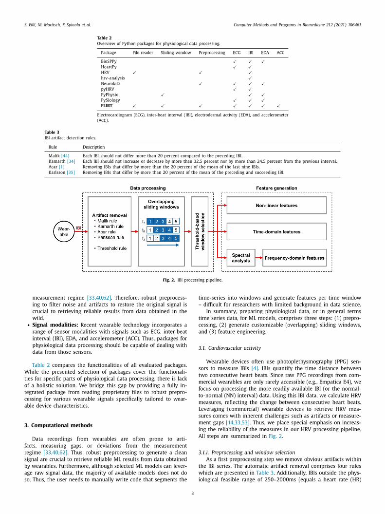
Fig. 2. IBI processing pipeline.

W

t

o

t

c

a

3

f

r

s

b

a

s

t

–

t

c

a

3

s

t

m

f

t

m

L

s

m

i

A

3

t

w

i

measurement regime [33,40,62] . Therefore, robust preprocess-

ing to filter noise and artifacts to restore the original signal is

crucial to retrieving reliable results from data obtained in the

wild. • Signal modalities: Recent wearable technology incorporates a

range of sensor modalities with signals such as ECG, inter-beat

interval (IBI), EDA, and accelerometer (ACC). Thus, packages for

physiological data processing should be capable of dealing with

data from those sensors.

Table 2 compares the functionalities of all evaluated packages.

hile the presented selection of packages cover the functionali-

ies for specific parts of physiological data processing, there is lack

f a holistic solution. We bridge this gap by providing a fully in-

egrated package from reading proprietary files to robust prepro-

essing for various wearable signals specifically tailored to wear-

ble device characteristics.

. Computational methods

Data recordings from wearables are often prone to arti-

acts, measuring gaps, or deviations from the measurement

egime [33,40,62] . Thus, robust preprocessing to generate a clean

ignal are crucial to retrieve reliable ML results from data obtained

y wearables. Furthermore, although selected ML models can lever-

ge raw signal data, the majority of available models does not do

o. Thus, the user needs to manually write code that segments the

3

ime-series into windows and generate features per time window

difficult for researchers with limited background in data science.

In summary, preparing physiological data, or in general terms

ime series data, for ML models, comprises three steps: (1) prepro-

essing, (2) generate customizable (overlapping) sliding windows,

nd (3) feature engineering.

.1. Cardiovascular activity

Wearable devices often use photoplethysmography (PPG) sen-

ors to measure IBIs [4] . IBIs quantify the time distance between

wo consecutive heart beats. Since raw PPG recordings from com-

ercial wearables are only rarely accessible (e.g., Empatica E4), we

ocus on processing the more readily available IBI (or the normal-

o-normal (NN) interval) data. Using this IBI data, we calculate HRV

easures, reflecting the change between consecutive heart beats.

everaging (commercial) wearable devices to retrieve HRV mea-

ures comes with inherent challenges such as artifacts or measure-

ent gaps [14,33,53] . Thus, we place special emphasis on increas-

ng the reliability of the measures in our HRV processing pipeline.

ll steps are summarized in Fig. 2 .

.1.1. Preprocessing and window selection

As a first preprocessing step we remove obvious artifacts within

he IBI series. The automatic artifact removal comprises four rules

hich are presented in Table 3 . Additionally, IBIs outside the phys-

ological feasible range of 250–20 0 0ms (equals a heart rate (HR)

S. Föll, M. Maritsch, F. Spinola et al. Computer Methods and Programs in Biomedicine 212 (2021) 106461

o

p

c

s

d

a

d

g

m

f

t

H

T

i

c

n

b

s

r

B

y

o

v

v

t

⌈

w

d

s

b

t

h

3

H

t

o

t

f

e

t

c

a

t

m

s

F

p

E

t

c

p

o

u

t

I

n

i

3

c

m

3

t

t

fi

l

a

m

r

s

g

x

w

c

n

t

t

l

e

s

m

S

m

P

w

i

g

a

i

d

P

s

p

s

x

w

vt

s

t

s

f 30–240) are discarded as well [55] . The cleaned IBIs are then

artitioned into overlapping time windows for feature generation.

The IBI series can contain measuring gaps caused by either dis-

arded (ectopic) beats or heart beats not recognized by the mea-

urement device; a frequent case with wearables [14,33] . Han-

ling missing data is an important step to avoid otherwise neg-

tively affected HRV measures [50,53] . This error in HRV features

rastically increases with the occurrence and length of measuring

aps [41,50] . However, applying interpolation methods to recover

issing beats can cause a significant proportion of errors in HRV

eatures whenever measuring gaps occur [50] . In contrast to in-

erpolation, incomplete time windows can be discarded prior to

RV feature calculation to prevent overly inaccurate measures [44] .

hus, instead of accepting an arbitrary error in HRV measures, we

ncrease the reliability of the HRV measure by defining a threshold

riterion for the removal of incomplete windows.

We do not rely on a static threshold such as the minimum

umber of sinus beats because it would imply two major draw-

acks. First, such approaches cannot be individualized to single

ubjects and, second, they are not dynamically adjusting to tempo-

al changes in the input signal (e.g., diurnal changes in heart rates).

ased on the idea of [14] , we introduce an adaptive threshold anal-

sis method. We set an adaptive threshold for a minimum number

f detected beats based on the expected number of beats per indi-

idual time window. The expected number of beats is estimated

ia the arithmetic mean over the detected heart beats within a

ime window.

A time window t is not discarded if it satisfies the inequality

thresh · L

μIBI t

⌉< N t ,

here L denotes the window length in seconds, N t the number of

etected valid beats in window t , μIBI t the mean IBI of window t in

econds, and thresh ∈ [0 , 1] the threshold, which can be chosen ar-

itrarily based on the desired application. In summary, the higher

he threshold is set the higher the required proportion of detected

eart beats with respect to the amount of expected beats.

.1.2. Feature engineering

Current research highlights three feature categories for

RV: statistical, time-domain, and frequency-domain fea-

ures [2,44,47,61,63,68] . In Table 4 , we summarize all features.

First, time-domain features represent the variability of the IBIs

ver a time specific period. Additionally, we retrieve the instan-

aneous heart rate from the IBIs and compute basic time domain

eatures. In case the wearable provides raw PPG data, one can gen-

rate statistical features for the blood volume pulse. In general,

ime-domain features are quickly calculable but provide less dis-

riminant power to distinguish between the two branches of the

utonomic nervous system [2] .

Second, frequency-domain features reflect the energy distribu-

ion over a range of frequencies. In particular, this class of HRV

easures better quantifies changes in the balance between the

ympathetic and parasympathetic autonomic nervous system [2] .

or frequency-domain HRV features, we have to estimate the

ower spectral density (PSD) of the partitioned IBI sequence [9] .

stimating PSD based on the fast Fourier transform requires an in-

erpolation method to produce an artificial equally-sampled dis-

rete time-series [9,38,44,58] . Since interpolation can affect the

ower spectrum, and thus frequency-domain features [50] , we rely

n the Lomb-Scargle method [42,57] . This method is robust against

nequally-sampled time-series and has shown promising results in

he context of HRV analysis [9,38,49] .

Third, non-linear HRV features quantify the uncertainty in the

BI sequence. We added them, since time- and feature-domain can-

4

ot account for the entire complexity of the mechanisms regulat-

ng HRV [58] .

.2. Electrodermal activity

In this section, we present an electrodermal activity (EDA) pro-

essing pipeline in order to retrieve reliable and standardized EDA

easures for ML applications. All steps are depicted in Fig. 3 .

.2.1. Preprocessing EDA

We present two distinct categories of approaches. First, two in-

egrated approaches which comprises artifact removal and noise fil-

ering: (a) the extended Kalman filter (EKF) and (b) the particle

lter (PF). Second, a modular approach which allows to combine

ow-pass filter and artifact detection algorithms.

Kalman filter The Kalman filter is an integrated, model-based

pproach for filtering data, which combines the data measure-

ents with a theoretical model of the signal to estimate its true

esponse. Our procedure implements the EKF algorithm as it has

hown reasonable results in removing noise and artifacts from data

athered using wearables [67] .

We estimate the state matrix as

= [ SC H , k di f f , SC 0 , SCR, S] T , (1)

here SC H is the hydration-dependent contribution to the skin

onductance (SC), SC 0 is the baseline SC of the inert skin, SCR de-

otes the skin conductance response (SCR), k di f f is the inverse

ime constant of the sweat diffusion, and the variable S denotes

he sudomotor nerve activation.

The model equations found in [67] are discretized and the non-

inear system is then linearized around the last predicted state in

ach time step. At each time step, the well-known Kalman filter

teps are performed: the prediction step (prior update) and the

easurement update (posterior update).

The final estimate of the SC signal is retrieved as SC = SC H +C 0 + SCR . Initialization was conducted according to [67] , with the

ean vector as x 0 = [0 , 0 , 0 , 0 , 0] T , and the variance as

0 =

⎡

⎢ ⎢ ⎣

0 . 01 0 0 0 0

0 0 . 01 0 0 0

0 0 0 . 01 0 0

0 0 0 0 . 001 0 . 01

0 0 0 0 . 01 0 . 01

⎤

⎥ ⎥ ⎦

,

here we slightly modified the variance of SC H , k di f f , and SC 0 . The

ntuition is that an over-idealized model may hinder the conver-

ence of the extended Kalman filter specifically when this filter is

pplied to real-world data.

Particle filter Similarly to the EKF, the PF is a model-based filter-

ng algorithm. However, PF assumes in contrast to EKF no normal

istribution of state and noise random variables. This allows the

F algorithm to be more widely applicable to wearable signals and

cenarios with highly non-Gaussian noise.

We propose a PF algorithm based on the pyParticleEst Python

ackage [54] . The algorithm is based on a linear process and mea-

urement model:

k +1 = x k + v k z k = x k + w k , (2)

here x k is the SC signal to estimate, z k is the EDA measurement,

k is the process noise and w k is the measurement noise, all at

ime k .

A specified number of particles are sampled from the initial

tate distribution to initialize the algorithm. Subsequently, the par-

icles are updated and propagated to the next time step by first

ampling from the prior distribution (the model) and then from

S. Föll, M. Maritsch, F. Spinola et al. Computer Methods and Programs in Biomedicine 212 (2021) 106461

Table 4

HR and HRV features.

Category Name Description Unit

Statistical min/max HR Minimum and maximum of the HR bpm

mean HR Mean of the HR i bpm

median HR Median of the HR i bpm

Time

domain

SDN N SD of all NN intervals ms

RMSSD The square root of the mean of the sum of the squares of differences between adjacent NN intervals ms

NN 50 Number of pairs of adjacent NN intervals differing by more than 50 ms in the entire recording ms

pNN 50 NN 50 count divided by the total number of all NN intervals %

NN 20 Number of pairs of adjacent NN intervals differing by more than 20 ms in the entire recording -

pNN 20 NN 20 count divided by the total number of all NN intervals. %

CV N N Coefficient of variation equal to the ratio of SDNN divided by mean NN interval -

CV SD Coefficient of variation of successive differences equal to the RMSSD divided by mean NN interval -

mean Mean of the IBIs ms

std Standard deviation of the IBIs ms

min/max Minimum and maximum of the IBIs ms

pt p Range (peak to peak) of the IBIs ms

sum Sum of the IBIs ms

energy Energy of the IBIs ms 2

skewness Skewness of the IBIs -

kurtosis Kurtosis of the IBIs -

peaks Number of the IBIs -

rms Root mean square of the IBIs ms

l ine _ integral Integral under the IBIs ms

n _ abov e _ mean Number of IBIs above the mean -

n _ below _ mean Number of IBIs below the mean -

n _ sign _ changes Number of changes in the IBIs slope -

iqr Interquartile range between the 25th and 75th percentile of the IBIs ms

iqr 5 − 95 Interquartile range between the 5th and 95th percentile of the IBIs ms

pct 5 5th percentile of the IBIs -

pct 95 95th percentile of the IBIs -

entropy Entropy of the IBIs -

perm entropy Permutation entropy of the IBIs -

s v d entropy Singular value decomposition of the IBIs entropy -

Frequency

domain

total power The variance of NN intervals over the temporal segment below 0.04 Hz ms 2

v l f Power in very low frequency range below or equal 0.04 Hz ms 2

l f Power in low frequency range 0.04 Hz and 0.15 Hz ms 2

h f Power in high frequency range 0.15 Hz and 0.4 Hz ms 2

l f/h f − ratio Ratio of LF to HF -

l f nu LF power in normalized units -

h f nu HF power in normalized units -

High frequency (HF), low frequency (LF), heart rate (HR), inter-beat interval (IBI), and normal-to-normal (NN) interval.

Fig. 3. EDA processing pipeline.

t

s

i

s

a

I

l

p

l

T

b

t

s

E

r

t

m

he posterior distribution (the measured SC signal). Additionally, a

moothing algorithm is applied to re-weight the particles, grant-

ng a larger contribution to the particles that better represent the

ignal.

Low-pass filter. The effect of measurement noise can be attenu-

ted by using a low-pass filter with the desired cut-off frequency.

n technical terms, a low-pass filter keeps only the frequencies be-

ow a specified threshold. Low-pass filtering is the traditional ap-

roach to automatically reduce noise in EDA signals [22,37,56] . We

everage several infinite impulse response filtering methods [69] .

5

he cutoff frequency is set below 0.5 Hz, since the SC signal is

and limited to 0.5 Hz [5] .

In contrast to the integrated approach, artifacts can be de-

ected and removed using ML algorithms as they have been proven

uccessful in automatically and accurately detecting artifacts in

DA signals recorded with wrist-worn devices [65,72] . In FLIRT,

esearchers can choose from the following two integrated, pre-

rained models:

EDAexplorer. Taylor et al. proposed this method, which detects

otion artifacts in the EDA raw data by classifying each consecu-

S. Föll, M. Maritsch, F. Spinola et al. Computer Methods and Programs in Biomedicine 212 (2021) 106461

Fig. 4. ACC processing pipeline.

t

s

c

t

d

c

t

t

t

e

t

c

i

I

r

3

t

w

c

m

a

b

n

s

c

S

s

n

e

t

m

w

i

m

b

t

a

3

t

t

r

t

v

o

d

s

i

n

C

w

i

o

n

w

t

o

p

r

e

p

l

g

f

o

w

t

c

3

c

I

i

t

t

w

c

3

s

w

ive five second epoch into artifact, questionable , or clean . The clas-

ification is performed using a support vector machine on features

omputed on the raw and low-pass filtered EDA data (for more de-

ailed information see [65] or [64] ).

Ideas-Lab UT. Further, we include a second method [72] that

etects motion artifacts in the raw EDA signal by classifying each

onsecutive five second epoch into artifact or clean . The classifica-

ion is performed using an logistic regression (LR) model on fea-

ures computed on the raw EDA data. The artifact detector was

rained on available labeled data, partially recorded in a controlled

nvironment and partially in-the-wild (for more detailed informa-

ion see [72] ).

These methods can be optionally enabled to optimize the out-

ome of EDA preprocessing. The methods’ performance in detect-

ng artifacts, however, may depend on the particular use case itself.

n both cases, the artifacts are marked and the resulting gap in the

aw EDA signal is linearly interpolated.

.2.2. Decomposition

The EDA signal consists of two SC components: skin conduc-

ance response (SCR) and skin conductance level (SCL) or in other

ords, the phasic and tonic component, respectively. Several de-

omposition algorithms for both components have been imple-

ented in the literature [6,8,13,26,29] . Below we elaborate on two

lgorithms for EDA signal decomposition that are included in FLIRT

ecause of their wide adoption, cvxEDA [26] and Ledalab [13] .

cvxEDA. The basic principle of cvxEDA is to model the EDA sig-

al as the sum of a SCR term, a SCL term, and additive white Gaus-

ian noise [26] . The algorithm then determines the SCR and SCL

omponents that maximize the likelihood of observing a specific

C time-series. The convex optimization problem is rewritten as a

tandard quadratic program, which can be solved efficiently.

Ledalab. The alternative Ledalab was chosen because it requires

o parameters other than the data itself and therefore can be gen-

ralized to all situations, without the need for additional parame-

er fine-tuning [13] . The key concept of the Ledalab algorithm is to

odel the SC signal as a sum of a SCR and SCL driver, convolved

ith an impulse response. This impulse response is modeled us-

ng the Bateman equation with parameters τ1 and τ2 (to be opti-

ized).

In presence of physiologically incoherent (nerve firing cannot

e negative) data, the SCR and SCL components can be further fil-

ered using a low-pass Butterworth filter to remove negative SCR

nd SCL values.

.2.3. Feature engineering

FLIRT computes general statistical and entropy features on both

he SCR and SCL components for each window. Time domain fea-

6

ures were chosen since they best describe the SCR and SCL signals

ecorded from wearable devices, as suggested by [24,28] . In con-

rast, frequency domain features of the EDA were proven to pro-

ide additional valuable information about the transient behaviour

f the sudomotor activity [3,24] . The benefits of time-frequency

omain features is that they capture the oscillatory behavior of the

udomotor response. Therefore, this class of features can provide

nformation to detect and distinguish health conditions [24] .

To calculate time-frequency domain features, the Cepstrum sig-

al C is estimated by [24]

= IF T (log| F T (X ) | ) , (3)

here X is the signal of interest, F T is Fourier Transform and IF T

s the inverse Fourier Transform. We are interested in the real part

f C, which gives us the required Mel-Frequency Cepstrum Compo-

ents as a basis of our features.

Peak features are computed only on the SCR component of each

indow. Table 6 shows a description of the calculated peak fea-

ures. We chose the best performing peak detection algorithms out

f [27,36,43,51,65] and implemented them in FLIRT: the EDAex-

lorer algorithm [64,65] and the algorithm implemented in Neu-

oKit2 [43] .

The EDAexplorer peak detection algorithm determines the pres-

nce of a peak based on several criteria related to a typical SCR

eak morphology such as the signal’s rate of change, maximum al-

owed rise time, and decay time. The Neurokit peak detection al-

orithm is based on the SciPy [69] Python package peak detection

unction. It refines its peak search by specifying constraints based

n the peaks derivative and on the density of peaks within a time-

indow.

Table 5 outlines the main parameters and their default values

hat can be individualized by the user. A detailed description of all

alculated features is presented in Table 6 .

.3. Accelerometer data

In addition to sensors that passively record physiological data,

ommercial wearables also have an embedded acceleration sensor.

n most cases a three-axis ACC is utilized, measuring accelerations

n the x-, y-, and z-axis. ACC data has been utilized for ML-based

asks such as human activity recognition or inferring physical ac-

ivity intensity [16,71] . Even physiological features calculated from

earable sensors such as HRV can be improved by taking into ac-

ount ACC information [18,45] .

.3.1. Preprocessing ACC

As outlined in prior work, filtering ACC data is an important

tep to reduce noise in the recordings. Although the number of

ays to filter the signal is many, there is a consensus in applying

S. Föll, M. Maritsch, F. Spinola et al. Computer Methods and Programs in Biomedicine 212 (2021) 106461

Table 5

Overview of parameters for EDA preprocessing. Corresponding default parameter values are indicated in parentheses.

Algorithm Available main parameter

Low-pass filter [69] cutoff (1e-1), filter (’butter’)

EKF [67] d_min (5e-3) d_max (5e-1), min_diff (1e-3), max_diff (1e-1), min_Savi_Go (-3e-2), max_Savi_Go (3e-2)

PF [54] num_particles (80), P0_variance (2-e2), Q_variance (2e-2), R_variance (6e-2)

EDAexplorer [65] –

Ideas-Lab UT [72] –

cvxEDA [26] delta_knot (15), cvx_alpha (8e-3), gamma (1e-3)

Ledalab [13] optimization (0)

EDAexplorer peaks [65] threshold (1e-2)

Neurokit peaks [43] amplitude_min (3e-2)

Table 6

EDA features.

Category Name Description Unit

Time

domain

mean Mean of the SCR and SCL μS

std Standard deviation of the SCR and SCL μS

min/max Minimum and maximum of the SCR and SCL μS

pt p Range (peak to peak) of SCR and SCL within a time interval μS

sum Sum of the SCR and SCL values with a time interval μS

energy Energy of the SCR and SCL μS 2

skewness Skewness of the SCR and SCL -

kurtosis Kurtosis of the SCR and SCL -

peaks Number of SCR and SCL peaks with a time interval -

rms Root mean square of the SCR and SCL μS

l ine _ integral Integral under the SCR and SCL curve μS.s

n _ abov e _ mean Number of SCR and SCL data-points above the mean -

n _ below _ mean Number of SCR and SCL data-points below the mean -

n _ sign _ changes Number of changes in the SCR and SCL slope -

iqr Interquartile range between the 25th and 75th percentile of the SCR and SCL μS

iqr _ 5 − 95 Interquartile range between the 5th and 95th percentile of the SCR and SCL μS

pct _ 5 5th percentile of the SCR and SCL -

pct _ 95 95th percentile of the SCR and SCL -

entropy Entropy of the SCR and SCL -

perm _ entropy Permutation entropy of the SCR and SCL -

s v d _ entropy Singular value decomposition of the SCR and SCL entropy -

Frequency

domain

sma Signal magnitude area of the frequency domain SCR and SCL μS

energy Energy of the frequency domain SCR and SCL μS 2

kurtosis Kurtosis of the frequency domain SCR and SCL -

iqr Interquartile range of the frequency domain SCR and SCL μS/Hz

spectral _ power 5 spectral power magnitudes in the [0.05-0.55] Hz bands for the power density of the SCR and SCL μS 2 .Hz

v ar _ power Variance of the SCR and SCL spectral power μS 2

Time-

frequency

domain

mean Mean of the SCR’s and SCL’s MFC signal μS

std Mean of the SCR’s and SCL’s MFC signal μS

median Median of the SCR’s and SCL’s MFC signal μS

iqr Interquartile range of the SCR’s and SCL’s MFC signal μS

skewness Skewness of the SCR’s and SCL’s MFC signal -

kurtosis Kurtosis of the SCR’s and SCL’s MFC signal -

SCR

time-

domain

features

peaks Number of SCR peaks -

rise _ time Mean of the SCR peaks rise time s

max _ deri v Mean value of the maximum derivative of the SCR peaks μS/s

amp Mean amplitude of the SCR peaks μS

decay _ time Mean of the SCR peaks decay time s

scr _ width Mean width of the SCR peaks s

auc _ mean Mean area-under-curves of the SCR peaks μS.s

auc _ sum Sum of the area-under-curves of the SCR peak μS.s

Mel-Frequency Cepstrum (MFC), skin conductance level (SCL), and skin conductance response (SCR).

l

w

3

c

d

t

t

n

F

f

e

s

f

4

v

g

t

p

ow-pass filters [20,30,70] . As suggested by Fridolfsson et al. [20] ,

e set the default cut-off frequency to 10 Hz.

.3.2. Feature engineering

For ACC, FLIRT provides an additional generic set of features

onsisting of time domain, frequency domain, and time-frequency

omain features [10,31,39,59] . We calculate this set of features on

he filtered ACC data. Following the idea of [59] , we computed

he set of features for each ACC axis and additionally on the l2-

orm of these three axes. Table 7 summarizes those features and

igure 4 depicts our ACC pipeline. Note that for the spectral power

eatures we chose the ranges according to Huynh et al. [31] and

7

stimated the Cepstrum signal with Eq. 3 . In addition, the generic

et of statistical features applied to ACC could as well be leveraged

or other sensor data such as temperature readings.

. Software description

FLIRT is implemented in Python and supports Python 3 with

ersions 3.7 and above. The package structure is shown in Table 8 .

We provide an extensive documentation of the application pro-

rammer interface (API) via the popular Sphinx Python documen-

ation tool. It translates source-code documentation markup into

retty, human-readable documentation. Furthermore, the API doc-

S. Föll, M. Maritsch, F. Spinola et al. Computer Methods and Programs in Biomedicine 212 (2021) 106461

Table 7

ACC features.

Category Name Description Unit

Time

domain

mean Mean of the ACC signal g

std Standard deviation of the ACC signal g

min/max Minimum and maximum of the ACC signal g

pt p Range (peak to peak) of the ACC signal g

sum Sum of the ACC signal g

energy Energy of the ACC signal g 2

skewness Skewness of the ACC signal -

kurtosis Kurtosis of the ACC signal -

peaks Number of the ACC signal -

rms Root mean square of the ACC signal g

l ine _ integral Integral under the ACC signal g

n _ abov e _ mean Number of ACC signal above the mean -

n _ below _ mean Number of ACC signal below the mean -

n _ sign _ changes Number of changes in the ACC signal slope -

iqr Interquartile range between the 25th and 75th percentile of the ACC signal g

iqr _ 5 − 95 Interquantile range between the 5th and 95th percentile of the ACC signal g

pct _ 5 5th percentile of the ACC signal -

pct _ 95 95th percentile of the ACC signal -

entropy Entropy of the ACC signal -

perm _ entropy Permutation entropy of the ACC signal -

s v d _ entropy Singular value decomposition of the ACC signal entropy -

Frequency

domain

sma Signal magnitude area of the frequency domain ACC signal g

energy Energy of the frequency domain ACC signal g 2

kurtosis Kurtosis of the frequency domain ACC signal -

iqr Interquartile range of the frequency domain ACC signal g/Hz

spectral _ power 3 spectral power magnitudes in the [1–5.5] Hz bands for the power density of the ACC signal g 2 .Hz

v ar _ power Variance of the ACC signal spectral power g 2

Time-

frequency

domain

mean Mean of the ACC signal’s MFC signal g

std Mean of the ACC signal’s MFC signal g

median Median of the ACC signal’s MFC signal g

iqr Interquartile range of the ACC signal’s MFC signal g

skewness Skewness of the ACC signal’s MFC signal -

kurtosis Kurtosis of the ACC signal’s MFC signal -

Accelerometer (ACC) and gravitational force equivalent (g).

Table 8

FLIRT software sub-packages.

Sub-package Description

flirt Provides access to most common functions ( get_eda_features, get_hrv_features, get_acc_features ).

flirt.reader Provides implementations to read common file formats such as Empatica E4 ( flirt.reader.empatica ) or Holter devices

( flirt.reader.holter ).

flirt.with_ Convenience sub-package to provide functions for commonly used methods. For example, for a ready Empatica E4 zip archive a function call

to flirt.with_.empatica('E4.zip') will automatically parse all available data and generate features.

flirt.eda Provides access to low-level feature functions for processing EDA data.

flirt.hrv Provides access to low-level feature functions for processing HRV data.

flirt.acc Provides access to low-level feature functions for processing ACC data.

flirt.stats Provides access to a standard set of statistical aggregation functions which will generate features in a window-based approach for arbitrary

time-series data.

u

T

s

a

i

a

f

l

d

q

e

c

i

5

o

p

d

c

t

R

t

i

i

S

w

d

mentation can easily be extended by custom pages like articles.

he documentation artifact is provided on the public readthedocs 9

ervice.

To facilitate fast and easy installation, we provide FLIRT via PyPI

nd it can easily be installed to Python environments via pip nstall flirt .

In its core, FLIRT uses parallelization wherever possible and

llows for multi-threaded execution. Specifically, FLIRT by de-

ault uses parallel multi-core processing for the feature generation

oops. Since the feature calculation process for each time window

oes not depend on information from other time windows, the se-

uence of execution is irrelevant and thus can be parallelized and

xecuted in an arbitrary order. Furthermore, when working with

omplex signal decomposition methods, we rely on already exist-

ng, vectorized implementations out of NumPy and SciPy [69] .

9 https://flirt.readthedocs.io

w

t

o

8

. Results and discussion

The objective of this section is to validate reproducible sets

f features provided by FLIRT . For this purpose, we rely on the

ublicly available Wearable Stress and Affect Detection (WESAD)

ataset and its classification performance as baseline [59] . WESAD

ontains wearable sensor data from 15 participants going through

ask-induced emotions. During the study, an Empatica E4 and a

espiBan sensor were used to record the physiological response to

he emotions relaxation, amusement, and stress. The Empatica E4

n particular is an established device whose data has been used

n a variety of published studies and articles [19] . Since the WE-

AD dataset defines a clear ML-task and baseline as well as uses a

idely established wearable, we will rely on this publicly available

ataset for validation.

Our validation follows the original WESAD paper. Nevertheless,

e found that reproducibility of their features was limited due

o incomplete information about the algorithms as well as a lack

f publicly available code. Therefore, we use the results from the

S. Föll, M. Maritsch, F. Spinola et al. Computer Methods and Programs in Biomedicine 212 (2021) 106461

Table 9

Classification performance on the WESAD dataset. The mean (standard deviation) of the respective macro F1-score over 5 randomly

initialized runs are reported. Note that LDA is a deterministic model and thus no standard deviation is reported. Best mean F1-scores are

highlighted in bold.

Parameters ML model

Artifact detection Window selection LDA RF AB DT

HRV WESAD – – 54.72 53.83 (0.11) 53.29 (0.16) 51.15 (0.31)

FLIRT default Malik rule threshold = 0.0 57.59 57.13 (0.59) 54.85 (0.77) 49.23 (1.12)

FLIRT threshold Malik rule threshold = 0.2 53.21 52.28 (0.43) 49.14 (1.36) 47.78 (0.64)

Data preprocessing Decomposition method

EDA WESAD – – 42.72 45.74 (0.06) 49.06 (0.59) 45.48 (0.17)

FLIRT integrated EKF cvxEDA 51.54 43.46 (0.34) 51.96 (0.32) 44.70 (0.45)

FLIRT modular B.worth, LR cvxEDA 50.43 42.17 (0.40) 51.02(0.43) 41.98 (0.32)

Data preprocessing

ACC WESAD - 36.27 46.50 (0.26) 46.38 (1.02) 43.91 (1.16)

FLIRT Unfiltered signal 56.55 55.58 (0.31) 55.92 (1.02) 52.99 (0.75)

FLIRT Butterworth filter 54.93 48.73 (0.24) 48.70 (0.47) 49.32 (0.35)

AdaBoost (AB), accelerometer (ACC), decision tree (DT), electrodermal activity (EDA),extended Kalman filter (EKF), inter-beat interval (IBI),

linear discriminant analysis (LDA), logistic regression (LR), machine learning (ML), and random forest (RF).

o

f

s

b

M

A

(

F

c

a

W

i

b

g

r

f

c

H

f

w

i

b

p

s

w

o

d

s

s

n

t

i

r

e

d

o

H

u

f

w

6

f

d

a

s

b

o

c

a

d

t

o

m

t

r

a

t

t

m

a

d

P

v

i

D

t

o

I

w

E

s

w

T

e

riginal paper as baseline. Second, we calculated all features uni-

ormly over a 60 seconds time window, 10 with a sliding window

hift of 1/4 seconds, and assigned the corresponding emotion la-

el to each window. For the classification task, we compare four

L models from the original WESAD paper (Random forest (RF),

daBoost (AB), decision tree (DT), and linear discriminant analysis

LDA)). Our objective is to compare the feature generation between

LIRT and WESAD in particular. Although emotion recognition is a

hallenging task and might require more complex ML models, we

im to be comparable to the ML pipeline presented in the original

ESAD paper, and thus we used the same models, parameters, and

mplementations. We report classification with the macro F1-score

ased on a leave-one-subject-out cross-validation to assess model

eneralization capabilities to unseen subjects. We summarize the

esults in Table 9 .

In general, FLIRT offers many ways to combine algorithms for

eature calculation. In this section, we evaluate the basic data pro-

essing options from which the user can choose. In the case of

RV, the F1-score increases by 2.87 pp for the overall best per-

orming RF model based on FLIRT’s default HRV features without

indow selection (i.e., threshold = 0). For the EDA modality, the

ntegrated EDA pipeline yields an overall improvement of 2.9 pp

ased on the LDA model. Finally, the ACC features achieve an im-

rovement of 10.05 pp for the LDA model. Although we used the

ame ML model hyperparameters as the original WESAD paper,

here the parameters were tuned to their feature sets, we achieve

verall better results than the WESAD baseline.

For the ACC features, we included FLIRT without filtering ACC

ata as presented in [59] . It is noticeable that ACC features achieve

trong improvements compared to the baseline. We see two rea-

ons for this improved performance. First, FLIRT calculates sig-

ificantly more features than WESAD (92 vs. 19). Second, emo-

ions in WESAD are task-induced, e.g., stress from public speak-

ng and amusement from watching a video. Therefore, it seems

easonable that our large set of ACC features simply captures the

motion-specific task (sitting vs. gesticulating) rather than the in-

uced emotion. However, there is a high likelihood that even the

riginal WESAD-based ACC classifications makes use of this Clever

ans strategy. In essence, the WESAD setting suggests to avoid the

se of ACC features and we only include this analysis to maintain

ull comparability to WESAD.

10 In general, WESAD uses 60 seconds as well, however, the authors change the

indow length for ACC to 5 seconds.

C

–

t

9

. Conclusion

In this paper, we presented FLIRT: A Feature Generation Toolkit

or Wearable Data , a Python package that focuses explicitly on stan-

ardized processing of physiological data from commercial wear-

bles, from data cleaning to feature extraction. FLIRT supports re-

earchers to leverage rich sensing data (HRV, EDA, ACC) obtained

y wearables to build ML models for various health and behavioral

utcome detections. Instead of writing custom code to preprocess,

lean, and compute features, which results in a lack of uniformity

cross studies, FLIRT helps researchers to create fast and repro-

ucible results across disciplines and applications with state-of-

he-art methods.

However, we tested FLIRT on a publicly available dataset based

n which we demonstrated an increase in classification perfor-

ance. Whether this increase can be achieved in other applica-

ions remains to be seen. However, note that FLIRT enables the

eproducibility of the results and contributes to research in this

rea. Last, applying FLIRT can inherit a challenge that is choosing

he parameters of FLIRT. Although we included default parameters

ailored to supported wearables (e.g., Empatica E4), the user must

anually tune these parameters for yet unsupported wearables.

Soon, we look forward to extending the capabilities of FLIRT,

nd welcome the community to this open-source project. Future

irections include a detailed performance comparison to related

ython packages, incorporating different commercial wearable de-

ices (e.g., Apple Watch), and increasing the functionalities with

mproved algorithms and feature selection capabilities.

eclaration of Competing Interest

T.K. and E.F. are affiliated with the Center for Digital Health In-

erventions ( www.c4dhi.org ), a joint initiative of the Department

f Management, Technology and Economics at ETH Zurich and the

nstitute of Technology Management at the University of St. Gallen,

hich is funded in part by the Swiss health insurer CSS. T.K. and

.F. are also co-founders of Pathmate Technologies, a university

pin-off company that creates and delivers digital clinical path-

ays. However, Pathmate Technologies is not involved in any way.

he remaining authors declare that they have no competing inter-

sts.

RediT authorship contribution statement

Simon Föll: Conceptualization, Methodology, Software, Writing

original draft, Project administration. Martin Maritsch: Concep-

ualization, Methodology, Software, Visualization, Writing – origi-

S. Föll, M. Maritsch, F. Spinola et al. Computer Methods and Programs in Biomedicine 212 (2021) 106461

n

i

F

K

v

&

A

2

R

[

[

[

[

[

[

[

[

[

[

[

[

[

[

[

[

[

[

[

[

[

[

[

[

al draft. Federica Spinola: Software, Visualization, Writing – orig-

nal draft. Varun Mishra: Validation, Writing – review & editing.

ilipe Barata: Methodology, Writing – review & editing. Tobias

owatsch: Writing – review & editing. Elgar Fleisch: Writing – re-

iew & editing. Felix Wortmann: Methodology, Writing – review

editing, Supervision.

cknowledgment

This work was part-funded by the Hasler Stiftung , Project

0039.

eferences

[1] B. Acar , I. Savelieva , H. Hemingway , M. Malik , Automatic ectopic beat elimina-

tion in short-term heart rate variability measurement, Comput Methods Pro- grams Biomed 63 (20 0 0) 123–131 .

[2] R.U. Acharya, P.K. Joseph, N. Kannathal, C.M. Lim, J.S. Suri, Heart rate variabil-

ity: a review, Med. Biol. Eng. Comput. 44 (12) (2006) 1031–1051, doi: 10.1007/ s11517- 006- 0119- 0 .

[3] A . Alberdi, A . Aztiria, A . Basarab, Towards an automatic early stress recognitionsystem for office environments based on multimodal measurements: a review,

J Biomed Inform 59 (2016) 49–75, doi: 10.1016/j.jbi.2015.11.007 . [4] J. Allen, Photoplethysmography and its application in clinical physiological

measurement, Physiol Meas 28 (3) (2007) 1–39, doi: 10.1088/0967-3334/28/3/

R01 . [5] M.R. Amin , R.T. Faghih , Inferring autonomic nervous system stimulation from

hand and foot skin conductance measurements, 2018, pp. 655–660 . [6] M.R. Amin, R.T. Faghih, Tonic and phasic decomposition of skin conduc-

tance data: A generalized-cross-validation-based block coordinate descent ap- proach, in: 41st Annual International Conference of the IEEE Engineering in

Medicine and Biology Society (EMBC), 2019, pp. 745–749, doi: 10.1109/EMBC. 2019.8857074 .

[7] R. Avram , J.E. Olgin , P. Kuhar , J.W. Hughes , G.M. Marcus , M.J. Pletcher , K. As-

chbacher , G.H. Tison , A digital biomarker of diabetes from smartphone-based vascular signals, Nat. Med. (2020) .

[8] D.R. Bach, K.J. Friston, R.J. Dolan, An improved algorithm for model-based anal- ysis of evoked skin conductance responses, Biol Psychol 94 (2013) 4 90–4 97,

doi: 10.1016/j.biopsycho.2013.09.010 . [9] M. Bachler, Spectral analysis of unevenly spaced data: models and application

in heart rate variability, SNE Simulation Notes Europe 27 (4) (2017) 183–190,

doi: 10.11128/sne.27.tn.10393 . URL: https://www.sne-journal.org/10383 [10] L. Bao, S.S. Intille, Activity recognition from user-annotated acceleration

data, Pervasive Computing, Springer Berlin Heidelberg, 2004, doi: 10.1007/ 978- 3- 540- 24646- 6 _ 1 .

[11] R. Bartels, hrv, 2020, [Online; accessed October 26, 2020], URL: https://hrv. readthedocs.io/en/latest/ .

[12] M.O. Bekkink, M. Koeneman, B.E. de Galan, S.J. Bredie, Early detection of hypo-

glycemia in type 1 diabetes using heart rate variability measured by a wear- able device, Diabetes Care 42 (4) (2019) 689–692, doi: 10.2337/dc18-1843 .

[13] M. Benedek, C. Kaernbach, Decomposition of skin conductance data by means of nonnegative deconvolution, Psychophysiology 47 (2010) 647–658, doi: 10.

1111/j.1469-8986.20 09.0 0972.x . [14] B. Bent, B.A. Goldstein, W.A. Kibbe, J.P. Dunn, Investigating sources of inaccu-

racy in wearable optical heart rate sensors, npj Digital Medicine 3 (1) (2020)

18, doi: 10.1038/s41746- 020- 0226- 6 . [15] A . Bizzego, A . Battisti, G. Gabrieli, G. Esposito, C. Furlanello, Pyphysio: a phys-

iological signal processing library for data science approaches in physiol- ogy, SoftwareX 10 (2019) 100287, doi: 10.1016/j.softx.2019.100287 . URL: http:

//www.sciencedirect.com/science/article/pii/S2352711019301839 [16] P. Casale , O. Pujol , P. Radeva , Human Activity Recognition from Accelerometer

Data Using a Wearable Device BT - Pattern Recognition and Image Analysis,

Springer Berlin Heidelberg, Berlin, Heidelberg, 2011, pp. 289–296 . [17] R. Champseix, hrv-analysis, 2020, [Online; accessed October 26, 2020], URL:

https://aura-healthcare.github.io/hrvanalysis/ . [18] E.P. Doheny, M.M. Lowery, A. Russell, S. Ryan, Estimation of respiration rate

and sleeping position using a wearable accelerometer, in: 2020 42nd Annual International Conference of the IEEE Engineering in Medicine & Biology Society

(EMBC), 2020, pp. 4668–4671, doi: 10.1109/EMBC44109.2020.9176573 .

[19] Empatica, Empatica - scientific publications, 2020, [Online; accessed October 26, 2020], URL: https://www.empatica.com/research/publications/ .

20] J. Fridolfsson, M. Börjesson, C. Buck, Ö. Ekblom, E. Ekblom-Bak, M. Hunsberger, L. Lissner, D. Arvidsson, Effects of frequency filtering on intensity and noise

in accelerometer-based physical activity measurements, Sensors 19 (9) (2019), doi: 10.3390/s19092186 .

[21] G. Gabrieli, Pysiology - physiological analysis made easy, 2020, [Online; ac- cessed October 26, 2020], URL: https://pysiology.readthedocs.io/en/latest/ .

22] S. Gashi , E.D. Lascio , B. Stancu , V.D. Swain , V. Mishra , M. Gjoreski , S. Santini ,

Detection of artifacts in ambulatory electrodermal activity data, Proc. ACM In- teract. Mob. Wearable Ubiquitous Technol. 4 (2020) .

23] P. van Gent, Python heart rate analysis toolkit, 2020, [Online; accessed Octo- ber 26, 2020], URL: https://python- heart- rate- analysis- toolkit.readthedocs.io/

en/latest/heartrateanalysis.html .

10

24] P. Ghaderyan, A. Abbasi, An efficient automatic workload estimation method based on electrodermal activity using pattern classifier combinations, Inter-

national Journal of Psychophysiology 110 (2016) 91–101, doi: 10.1016/j.ijpsycho. 2016.10.013 .

25] P. Gomes, Pyhrv - python toolbox for heart rate variability, 2020, [Online; accessed October 26, 2020], URL: https://pyhrv.readthedocs.io/en/latest/index.

html . 26] A. Greco, G. Valenza, A. Lanata, E.P. Scilingo, L. Citi, Cvxeda: a convex optimiza-

tion approach to electrodermal activity processing, IEEE Trans. Biomed. Eng. 63

(2016) 797–804, doi: 10.1109/TBME.2015.2474131 . 27] S. Halem, E. Roekel, L. Kroencke, N. Kuper, J. Denissen, Moments that mat-

ter? on the complexity of using triggers based on skin conductance to sam- ple arousing events within an experience sampling framework, Eur J Pers 34

(2020), doi: 10.1002/per.2252 . 28] J.A. Healey, R.W. Picard, Detecting stress during real-world driving tasks using

physiological sensors, IEEE Trans. Intell. Transp. Syst. 6 (2005) 156–166, doi: 10.

1109/TITS.2005.84 836 8 . 29] F. Hernando-Gallego, D. Luengo, A. Artes-Rodriguez, Feature extraction of gal-

vanic skin responses by nonnegative sparse deconvolution, IEEE J Biomed Health Inform 22 (2018) 1385–1394, doi: 10.1109/JBHI.2017.2780252 .

30] M. Huang, G. Zhao, L. Wang, F. Yang, A pervasive simplified method for human movement pattern assessing, in: 2010 IEEE 16th International Conference on

Parallel and Distributed Systems, 2010, pp. 625–628, doi: 10.1109/ICPADS.2010.

65 . [31] Q.T. Huynh , U.D. Nguyen , B.Q. Tran , Power spectral analyses to detect falls us-

ing 3-d accelerometers, in: T. Vo Van, T.A. Nguyen Le, T. Nguyen Duc (Eds.), 6th International Conference on the Development of Biomedical Engineering

in Vietnam (BME6), Springer Singapore, Singapore, 2018, pp. 191–195 . 32] N.C. Jacobson, H. Weingarden, S. Wilhelm, Digital biomarkers of mood disor-

ders and symptom change, npj Digital Medicine 2 (1) (2019) 3, doi: 10.1038/

s41746- 019- 0078- 0 . 33] E. Jovanov, Preliminary analysis of the use of smartwatches for longitudi-

nal health monitoring, in: 2015 37th Annual International Conference of the IEEE Engineering in Medicine and Biology Society (EMBC), 2015, pp. 865–868,

doi: 10.1109/EMBC.2015.7318499 . 34] M. Kamath , E. Fallen , Correction Ofthe Heart Rate Variability Signal for Ectopics

and Missing Beats, in: M. Malik, A. Camm (Eds.), Heart Rate Variability, Futura

Pub. Co. Inc., Armonk, N.Y., 1995, pp. 75–85 . 35] M. Karlsson, R. Hörnsten, A. Rydberg, U. Wiklund, Automatic filtering of out-

liers in RR intervals before analysis of heart rate variability in holter record- ings: a comparison with carefully edited data, Biomed Eng Online 11 (1) (2012)

2, doi: 10.1186/1475-925X-11-2 . 36] K.H. Kim, S.W. Bang, S.R. Kim, Emotion recognition system using short-term

monitoring of physiological signals, Medical & Biological Engineering & Com-

puting 42 (2004), doi: 10.1007/BF02344719 . 37] I.R. Kleckner , R.M. Jones , O. Wilder-Smith , J.B. Wormwood , M. Akcakaya ,

K.S. Quigley , C. Lord , M.S. Goodwin , Simple, transparent, and flexible auto- mated quality assessment procedures for ambulatory electrodermal activity

data, IEEE Trans. Biomed. Eng. 65 (2018) 1460–1467 . 38] P. Laguna, G. Moody, R. Mark, Power spectral density of unevenly sampled

data by least-square analysis: performance and application to heart rate sig- nals, IEEE Trans. Biomed. Eng. 45 (6) (1998) 698–715, doi: 10.1109/10.678605 .

39] O.D. Lara, M.A. Labrador, A survey on human activity recognition using wear-

able sensors, IEEE Communications Surveys Tutorials 15 (3) (2013) 1192–1209, doi: 10.1109/SURV.2012.110112.00192 .

40] F. Larradet, R. Niewiadomski, G. Barresi, D.G. Caldwell, L.S. Mattos, Toward emotion recognition from physiological signals in the wild: approaching the

methodological issues in real-Life data collection, Front Psychol 11 (2020) 1111, doi: 10.3389/fpsyg.2020.01111 . URL: https://www.frontiersin.org/article/10.

3389/fpsyg.2020.01111

[41] N. Lippman, K.M. Stein, B.B. Lerman, Comparison of methods for removal of ec- topy in measurement of heart rate variability, American Journal of Physiology-

Heart and Circulatory Physiology 267 (1) (1994) H411–H418, doi: 10.1152/ ajpheart.1994.267.1.H411 . PMID: 7519408

42] N.R. Lomb, Least-squares frequency analysis of unequally spaced data, Astro- phys Space Sci 39 (2) (1976) 447–462, doi: 10.10 07/BF0 0648343 .

43] D. Makowski, T. Pham, Z.J. Lau, J.C. Brammer, F. Lespinasse, H. Pham,

C. Schölzel, S.H. Annabel Chen, Neurokit2: A python toolbox for neurophysi- ological signal processing, Zenodo, 2020, doi: 10.5281/ZENODO.3597887 . URL:

https://github.com/neuropsychology/NeuroKit 44] M. Malik, J.T. Bigger, A.J. Camm, R.E. Kleiger, A. Malliani, A.J. Moss,

P.J. Schwartz, Heart rate variability: standards of measurement, physiological interpretation, and clinical use, Eur. Heart J. 17 (3) (1996) 354–381, doi: 10.

1093/oxfordjournals.eurheartj.a014 86 8 .

45] M. Maritsch, C. Bérubé, M. Kraus, V. Lehmann, T. Züger, S. Feuerriegel, T. Kowatsch, F. Wortmann, Improving heart rate variability measurements from

consumer smartwatches with machine learning, in: Adjunct Proceedings of the 2019 ACM International Joint Conference on Pervasive and Ubiquitous Comput-

ing and Proceedings of the 2019 ACM International Symposium on Wearable Computers, in: UbiComp/ISWC ’19 Adjunct, Association for Computing Machin-

ery, New York, NY, USA, 2019, pp. 934–938, doi: 10.1145/3341162.3346276 .

46] M. Maritsch , S. Föll , V. Lehmann , C. Bérubé, M. Kraus , S. Feuerriegel ,T. Kowatsch , T. Züger , C. Stettler , E. Fleisch , et al. , Towards wearable-based hy-

poglycemia detection and warning in diabetes, in: Extended Abstracts of the 2020 CHI Conference on Human Factors in Computing Systems, 2020, pp. 1–8 .

S. Föll, M. Maritsch, F. Spinola et al. Computer Methods and Programs in Biomedicine 212 (2021) 106461

[

[

[

[

[

[

[

[

[

[

[

[

[

[

[

[

[

[

[

[

[

[

[

[47] J.E. Mietus, C.-K. Peng, I. Henry, R.L. Goldsmith, A.L. Goldberger, The pnnx files: re-examining a widely used heart rate variability measure, Heart 88 (4) (2002)

378–380, doi: 10.1136/heart.88.4.378 . 48] V. Mishra, S. Sen, G. Chen, T. Hao, J. Rogers, C.-H. Chen, D. Kotz, Evaluating

the reproducibility of physiological stress detection models, Proc. ACM Interact. Mob. Wearable Ubiquitous Technol. 4 (4) (2020), doi: 10.1145/3432220 .

49] G. Moody, Spectral analysis of heart rate without resampling, in: Proceed- ings of Computers in Cardiology Conference, IEEE Comput. Soc. Press, 1993,

pp. 715–718, doi: 10.1109/CIC.1993.378302 .

50] D. Morelli, A. Rossi, M. Cairo, D.A. Clifton, Analysis of the impact of interpo- lation methods of missing RR-intervals caused by motion artifacts on HRV

features estimations, Sensors 19 (14) (2019) 1–14, doi: 10.3390/s19143163 . URL: https://www.ncbi.nlm.nih.gov/pubmed/31323850 https://www.ncbi.nlm.nih.

gov/pmc/articles/PMC6679245/ https://www.mdpi.com/1424-8220/19/14/3163 [51] M. Nabian, Y. Yin, J. Wormwood, K.S. Quigley, L.F. Barrett, S. Ostadabbas, An

open-source feature extraction tool for the analysis of peripheral physiological

data, IEEE J Transl Eng Health Med 6 (2018), doi: 10.1109/JTEHM.2018.28780 0 0 . 52] A. Natarajan, H.-W. Su, C. Heneghan, Assessment of physiological signs associ-

ated with COVID-19 measured using wearable devices, npj Digital Medicine 3 (1) (2020) 156, doi: 10.1038/s41746- 020- 00363- 7 .

53] B.W. Nelson, C.A. Low, N. Jacobson, P. Areán, J. Torous, N.B. Allen, Guidelines for wrist-worn consumer wearable assessment of heart rate in biobehavioral re-

search, npj Digital Medicine 3 (1) (2020) 90, doi: 10.1038/s41746- 020- 0297- 4 .

54] J. Nordh, K. Berntorp, B. Nizette, pyparticleest, 2018, URL: https://github.com/ jerkern/pyParticleEst .

55] C. Orphanidou, T. Bonnici, P. Charlton, D. Clifton, D. Vallance, L. Tarassenko, Sig- nal quality indices for the electrocardiogram and photoplethysmogram: deriva-

tion and applications to wireless monitoring, IEEE J Biomed Health Inform 19 (3) (2014), doi: 10.1109/JBHI.2014.2338351 . 1–1, URL: http://ieeexplore.ieee.org/

document/6862843/

56] H.F. Posada-Quintero , K.H. Chon , Innovations in electrodermal activity data col- lection and signal processing: A systematic review, volume 20, MDPI AG, 2020 .

57] J.D. Scargle, Studies in astronomical time series analysis. II - statistical aspects of spectral analysis of unevenly spaced data, Astrophys. J. 263 (1982) 835,

doi: 10.1086/160554 . 58] T. Schaffer, B. Hensel, C. Weigand, J. Schüttler, C. Jeleazcov, Evaluation of

techniques for estimating the power spectral density of RR-intervals under

paced respiration conditions, J Clin Monit Comput 28 (5) (2014) 4 81–4 86, doi: 10.1007/s10877- 013- 9447- 4 .

59] P. Schmidt, A. Reiss, R. Duerichen, K.V. Laerhoven, Introducing wesad, a mul- timodal dataset for wearable stress and affect detection, ICMI 2018 - Proceed-

ings of the 2018 International Conference on Multimodal Interaction (2018) 400–408, doi: 10.1145/3242969.3242985 .

60] P. Schwab, W. Karlen, A deep learning approach to diagnosing multiple sclero-

sis from smartphone data, IEEE J Biomed Health Inform 25 (4) (2021) 1284–1291, doi: 10.1109/JBHI.2020.3021143 .

11

61] F. Shaffer, J.P. Ginsberg, An overview of heart rate variability metrics and norms, Front Public Health 5 (2017) 1–17, doi: 10.3389/fpubh.2017.00258 . URL:

http://journal.frontiersin.org/article/10.3389/fpubh.2017.00258/full 62] L. Smital, C.R. Haider, M. Vitek, P. Leinveber, P. Jurak, A. Nemcova, R. Smisek,

L. Marsanova, I. Provaznik, C.L. Felton, B.K. Gilbert, D.R.H. III, Real-Time quality assessment of long-term ECG signals recorded by wearables in free-living con-

ditions, IEEE Trans. Biomed. Eng. 67 (10) (2020) 2721–2734, doi: 10.1109/TBME. 2020.2969719 .

63] J.P. Spiers, B. Silke, U. McDermott, R.G. Shanks, D.W.G. Harron, Time and fre-

quency domain assessment of heart rate variability: a theoretical and clinical appreciation, Clinical Autonomic Research 3 (2) (1993) 145–158, doi: 10.1007/

BF018190 0 0 . 64] S. Taylor, N. Jaques, W. Chen, S. Fedor, A. Sano, R. Picard, Automatic identi-

fication of artifacts in electrodermal activity data, 2015a, ( https://github.com/ MITMediaLabAffectiveCom puting/eda-explorer a).

65] S. Taylor, N. Jaques, W. Chen, S. Fedor, A. Sano, R. Picard, Automatic iden-

tification of artifacts in electrodermal activity data, volume 2015-November, Institute of Electrical and Electronics Engineers Inc., 2015, pp. 1934–1937,

doi: 10.1109/EMBC.2015.7318762 . 66] Instituto de Telecomunicacoes, Biosppy - biosignal processing written in

python, 2020, [Online; accessed October 26, 2020], URL: https://biosppy. readthedocs.io/en/stable/ .

67] C. Tronstad, O.M. Staal, S. Saelid, O.G. Martinsen, Model- based filtering for

artifact and noise suppression with state estimation for electrodermal activ- ity measurements in real time, volume 2015-November, Institute of Electrical

and Electronics Engineers Inc., 2015, pp. 2750–2753, doi: 10.1109/EMBC.2015. 7318961 .

68] H.J. Van Dellen , J. Aasman , L.J.M. Mulder , G. Mulder , Time domain versus fre-quency domain measures of heart-rate variability, in: J.F. Orlebeke, G. Mulder,

L.J.P. Van Doornen (Eds.), Psychophysiology of Cardiovascular Control. Models,

Methods, and Data, Plenum Press, New York, 1985, pp. 353–374 . 69] P. Virtanen, R. Gommers, T.E. Oliphant, M. Haberland, T. Reddy, D. Courna-

peau, E. Burovski, P. Peterson, W. Weckesser, J. Bright, S.J. van der Walt, M. Brett, J. Wilson, K.J. Millman, N. Mayorov, A.R.J. Nelson, E. Jones, R. Kern,

E. Larson, C.J. Carey, I. Polat, Y. Feng, E.W. Moore, J. VanderPlas, D. Laxalde,J. Perktold, R. Cimrman, I. Henriksen, E.A. Quintero, C.R. Harris, A.M. Archibald,

A.H. Ribeiro, F. Pedregosa, P. van Mulbregt, SciPy 1.0 Contributors, Scipy 1.0:

fundamental algorithms for scientific computing in python, Nat. Methods 17 (2020) 261–272, doi: 10.1038/s41592- 019- 0686- 2 .

70] W.-Z. Wang, B.-Y. Huang, L. Wang, Analysis of filtering methods for 3d acceler- ation signals in body sensor network (2011). 10.1109/ISBB.2011.6107697

[71] C.-C. Yang, Y.-L. Hsu, A Review of Accelerometry-Based Wearable Mo- tion Detectors for Physical Activity Monitoring, Sensors, 2010, doi: 10.3390/

s100807772 .

72] Y. Zhang, M. Haghdan, K.S. Xu, Unsupervised motion artifact detection in wrist- measured electrodermal activity data. arXiv:1707.08287 .