Computer Aided Problem Solving

Carl Sandrock

2008

Contents

1 Computability and computers 11.1 Introduction . . . . . . . . . . . . . . . . . . . . . . . . . . . . . . . . . . 11.2 Equations . . . . . . . . . . . . . . . . . . . . . . . . . . . . . . . . . . . 11.3 Questions and problems . . . . . . . . . . . . . . . . . . . . . . . . . . . 2

1.3.1 Black boxes . . . . . . . . . . . . . . . . . . . . . . . . . . . . . . 21.4 Mathematical notation . . . . . . . . . . . . . . . . . . . . . . . . . . . . 31.5 Algorithm . . . . . . . . . . . . . . . . . . . . . . . . . . . . . . . . . . . 31.6 Computability . . . . . . . . . . . . . . . . . . . . . . . . . . . . . . . . . 71.7 Logic functions . . . . . . . . . . . . . . . . . . . . . . . . . . . . . . . . 7

1.7.1 Axioms . . . . . . . . . . . . . . . . . . . . . . . . . . . . . . . . 71.7.2 Black box abstraction . . . . . . . . . . . . . . . . . . . . . . . . 81.7.3 Reduction rules . . . . . . . . . . . . . . . . . . . . . . . . . . . . 91.7.4 Systematic reduction of logic expressions . . . . . . . . . . . . . . 9

2 Functional composition 112.1 Functions in computers . . . . . . . . . . . . . . . . . . . . . . . . . . . . 112.2 The current directory . . . . . . . . . . . . . . . . . . . . . . . . . . . . . 132.3 Comparisons . . . . . . . . . . . . . . . . . . . . . . . . . . . . . . . . . . 132.4 Conditionals . . . . . . . . . . . . . . . . . . . . . . . . . . . . . . . . . . 142.5 Recursion . . . . . . . . . . . . . . . . . . . . . . . . . . . . . . . . . . . 16

2.5.1 Calling yourself . . . . . . . . . . . . . . . . . . . . . . . . . . . . 162.5.2 More examples . . . . . . . . . . . . . . . . . . . . . . . . . . . . 172.5.3 Recursion rules . . . . . . . . . . . . . . . . . . . . . . . . . . . . 20

2.6 Assignments . . . . . . . . . . . . . . . . . . . . . . . . . . . . . . . . . . 20

3 Debugging 213.1 Introduction . . . . . . . . . . . . . . . . . . . . . . . . . . . . . . . . . . 213.2 Types of errors . . . . . . . . . . . . . . . . . . . . . . . . . . . . . . . . 21

3.2.1 Syntax errors . . . . . . . . . . . . . . . . . . . . . . . . . . . . . 213.2.2 Semantic errors . . . . . . . . . . . . . . . . . . . . . . . . . . . . 23

3.3 Pre-emptive maintainence . . . . . . . . . . . . . . . . . . . . . . . . . . 233.3.1 Comment . . . . . . . . . . . . . . . . . . . . . . . . . . . . . . . 233.3.2 Indent . . . . . . . . . . . . . . . . . . . . . . . . . . . . . . . . . 243.3.3 Space . . . . . . . . . . . . . . . . . . . . . . . . . . . . . . . . . 243.3.4 Parenthesise . . . . . . . . . . . . . . . . . . . . . . . . . . . . . . 243.3.5 Aim for readability . . . . . . . . . . . . . . . . . . . . . . . . . . 243.3.6 Keep functions short . . . . . . . . . . . . . . . . . . . . . . . . . 25

3.4 Tools and tricks . . . . . . . . . . . . . . . . . . . . . . . . . . . . . . . . 25

1

3.4.1 Octave . . . . . . . . . . . . . . . . . . . . . . . . . . . . . . . . . 253.4.2 Excel . . . . . . . . . . . . . . . . . . . . . . . . . . . . . . . . . . 25

4 Variables and types 274.1 Introduction . . . . . . . . . . . . . . . . . . . . . . . . . . . . . . . . . . 274.2 Variables . . . . . . . . . . . . . . . . . . . . . . . . . . . . . . . . . . . . 27

4.2.1 Scalar variables . . . . . . . . . . . . . . . . . . . . . . . . . . . . 274.2.2 Scope . . . . . . . . . . . . . . . . . . . . . . . . . . . . . . . . . 284.2.3 Vectors and matrices . . . . . . . . . . . . . . . . . . . . . . . . . 294.2.4 Concatenation . . . . . . . . . . . . . . . . . . . . . . . . . . . . . 304.2.5 Ranges . . . . . . . . . . . . . . . . . . . . . . . . . . . . . . . . . 304.2.6 Application . . . . . . . . . . . . . . . . . . . . . . . . . . . . . . 324.2.7 Exploration . . . . . . . . . . . . . . . . . . . . . . . . . . . . . . 34

4.3 Types . . . . . . . . . . . . . . . . . . . . . . . . . . . . . . . . . . . . . 344.3.1 Concept . . . . . . . . . . . . . . . . . . . . . . . . . . . . . . . . 344.3.2 Complex values . . . . . . . . . . . . . . . . . . . . . . . . . . . . 344.3.3 Strings . . . . . . . . . . . . . . . . . . . . . . . . . . . . . . . . . 354.3.4 Function handles . . . . . . . . . . . . . . . . . . . . . . . . . . . 37

4.4 Cell arrays . . . . . . . . . . . . . . . . . . . . . . . . . . . . . . . . . . . 374.4.1 The problem . . . . . . . . . . . . . . . . . . . . . . . . . . . . . . 374.4.2 The solution . . . . . . . . . . . . . . . . . . . . . . . . . . . . . . 384.4.3 Brackets and braces . . . . . . . . . . . . . . . . . . . . . . . . . . 384.4.4 Cell arrays and strings . . . . . . . . . . . . . . . . . . . . . . . . 39

4.5 Dealing with data . . . . . . . . . . . . . . . . . . . . . . . . . . . . . . . 404.5.1 Load and save . . . . . . . . . . . . . . . . . . . . . . . . . . . . . 404.5.2 Importing data . . . . . . . . . . . . . . . . . . . . . . . . . . . . 40

4.6 Assignments . . . . . . . . . . . . . . . . . . . . . . . . . . . . . . . . . . 40

5 Loops 465.1 Imperative algorithms . . . . . . . . . . . . . . . . . . . . . . . . . . . . 465.2 Types of iteration . . . . . . . . . . . . . . . . . . . . . . . . . . . . . . . 46

5.2.1 Deterministic loops . . . . . . . . . . . . . . . . . . . . . . . . . . 475.2.2 Non-deterministic loops . . . . . . . . . . . . . . . . . . . . . . . 48

5.3 Different ways of repeating . . . . . . . . . . . . . . . . . . . . . . . . . . 495.4 Roles of variables . . . . . . . . . . . . . . . . . . . . . . . . . . . . . . . 49

5.4.1 Concept . . . . . . . . . . . . . . . . . . . . . . . . . . . . . . . . 495.4.2 Fixed value . . . . . . . . . . . . . . . . . . . . . . . . . . . . . . 505.4.3 Stepper . . . . . . . . . . . . . . . . . . . . . . . . . . . . . . . . 505.4.4 Temporary . . . . . . . . . . . . . . . . . . . . . . . . . . . . . . . 505.4.5 Most-wanted holder . . . . . . . . . . . . . . . . . . . . . . . . . . 505.4.6 Gatherer . . . . . . . . . . . . . . . . . . . . . . . . . . . . . . . . 51

5.5 Assignments . . . . . . . . . . . . . . . . . . . . . . . . . . . . . . . . . . 51

6 Engineering problem solving 556.1 Introduction . . . . . . . . . . . . . . . . . . . . . . . . . . . . . . . . . . 556.2 Visualisation . . . . . . . . . . . . . . . . . . . . . . . . . . . . . . . . . . 55

6.2.1 Two dimensions . . . . . . . . . . . . . . . . . . . . . . . . . . . . 566.2.2 Three dimensions . . . . . . . . . . . . . . . . . . . . . . . . . . . 576.2.3 Annotations . . . . . . . . . . . . . . . . . . . . . . . . . . . . . . 57

2

6.3 Getting a handle on functions . . . . . . . . . . . . . . . . . . . . . . . . 596.3.1 Function handles . . . . . . . . . . . . . . . . . . . . . . . . . . . 596.3.2 Anonymous functions . . . . . . . . . . . . . . . . . . . . . . . . . 59

6.4 Curve fitting . . . . . . . . . . . . . . . . . . . . . . . . . . . . . . . . . . 606.4.1 Excel . . . . . . . . . . . . . . . . . . . . . . . . . . . . . . . . . . 606.4.2 Polynomials . . . . . . . . . . . . . . . . . . . . . . . . . . . . . . 606.4.3 Other curves . . . . . . . . . . . . . . . . . . . . . . . . . . . . . 61

6.5 Data lookup . . . . . . . . . . . . . . . . . . . . . . . . . . . . . . . . . . 616.5.1 Excel . . . . . . . . . . . . . . . . . . . . . . . . . . . . . . . . . . 626.5.2 Octave . . . . . . . . . . . . . . . . . . . . . . . . . . . . . . . . . 62

6.6 Integration . . . . . . . . . . . . . . . . . . . . . . . . . . . . . . . . . . . 626.6.1 Quadrature . . . . . . . . . . . . . . . . . . . . . . . . . . . . . . 626.6.2 Polynomials . . . . . . . . . . . . . . . . . . . . . . . . . . . . . . 63

6.7 Solving equations . . . . . . . . . . . . . . . . . . . . . . . . . . . . . . . 646.7.1 Polynomials . . . . . . . . . . . . . . . . . . . . . . . . . . . . . . 646.7.2 Sets of linear equations . . . . . . . . . . . . . . . . . . . . . . . . 646.7.3 Nonlinear equations . . . . . . . . . . . . . . . . . . . . . . . . . . 656.7.4 Sets of nonlinear equations . . . . . . . . . . . . . . . . . . . . . . 656.7.5 Excel Solver . . . . . . . . . . . . . . . . . . . . . . . . . . . . . . 66

6.8 Assignments . . . . . . . . . . . . . . . . . . . . . . . . . . . . . . . . . . 66

A Number systems and theory 70A.1 Value vs representation . . . . . . . . . . . . . . . . . . . . . . . . . . . . 70A.2 Numeral systems . . . . . . . . . . . . . . . . . . . . . . . . . . . . . . . 70

A.2.1 Radix conversion . . . . . . . . . . . . . . . . . . . . . . . . . . . 71A.2.2 Computer terminology . . . . . . . . . . . . . . . . . . . . . . . . 71A.2.3 IEEE floating point representation . . . . . . . . . . . . . . . . . 72A.2.4 Logic turns to math . . . . . . . . . . . . . . . . . . . . . . . . . 72

A.3 Assignments . . . . . . . . . . . . . . . . . . . . . . . . . . . . . . . . . . 73

3

Introduction

Engineers encounter problems every day. Many of these problems require a large numberof relatively simple operations to be carried out very accurately. Computers excel at suchtasks, and it is only natural that we should employ them to lighten our workload. In thisdocument, you are going to learn how to solve your engineering problems using a computerprogramming language called GNU Octave and a spreadsheet program called MicrosoftExcel. You will learn how to describe problems in such a way that using a computerto solve them becomes easier and you will learn some aspects of solving problems oncomputer that you may not have encountered while solving problems by hand.

This is the primary, but not the only reference for the subject CRV 210. You shouldread the recommended sections of the GNU Octave manual and the online help systemsfor the software when directed to do so.

Bear in mind that writing a computer program is not like using software that hasalready been designed to make your job easy. Learning to write computer programs issometimes frustrating and often confusing but the final result is not only very rewarding,but will make you a more efficient engineer.

4

Chapter 1

Computability and computers

Computers are useless. They can only give you answers.

Pablo Picasso

After completing this chapter you should be able to

• Use the correct nomenclature when describing problems.

• Explain the concept of a computable function

• Understand the concept of an algorithm as a solution to problems.

• Know and apply Boolean algebra concepts

• Derive a logic expression from a truth table and

• Simplify that expression using Boolean algebra axioms

1.1 Introduction

Think about answering an engineering question in a paper. A part of the knowledge thatyou are employing is about facts that you remember, such as multiplication tables or thesequence of the alphabet and spelling of words. This is called declarative knowledge.Another part is about how to do things, like spelling a word you have not yet seen, orcalculating 1234×3423. This knowledge is called procedural knowledge. We can onlyremember a limited number of facts, but if we know how to solve a problem, we can findthe answer to an infinite number of questions.

In many ways, computers are like genies. They interpret each of our commandsliterally, and they sometimes seem to want to misinterpret our commands. To makesure that there are no misunderstandings, we need to be very exact about describing ourproblems. Unfortunately, we will need to define some basic nomenclature.

This chapter deals with this nomenclature, covering some of the difficulties of usingconventional mathematical concepts to express processes rather than statements of truth.

1.2 Equations

Let’s start with something that probably doesn’t feel like a process – an explicit equation.

x = 1 + 2× 3 (1.1)

1

In Octave, we can enter this directly at the octave> prompt, using * instead of ×.

octave:1> x = 1 + 2*3

x = 7

In Excel, we can enter =1+2*3 , and the answer will be displayed in the cell when wepress enter.

A lot of action is going on behind the scenes of this equation – we need to know therules of precedence to multiply before adding, and we need to understand that x (or thecell) now has a value associated with it. All of that with just 6 symbols!

Things get a bit more interesting than explicit equations. Consider the followingequation:

2y = y + 2 (1.2)

Even though most of us can easily see that this implies that y = 2, there is no wayin either Octave or Excel to enter this equation as is. This is because there is a processinvolved in solving this equation. Notice, however that there is only one correct answer.

1.3 Questions and problems

We will be using the word question to refer to a specific problem with all the numbersfilled in. Examples of questions are “what is 1 added to 1?” or “what is the square rootof two?”. Clearly answer applies naturally to this. As we have seen, if we can find anexplicit equation that describes the question, we can enter it directly into Octave or Excelto find the answer. You should also notice that these questions can be answered frommemory, in other words using only declarative knowledge.

Now, we can generalise these questions as “how does one add two numbers together?”and “how does one determine the square root of a number?”. We will call the generalcase a problem. The solution to a problem will usually be a process, because eventhough you may remember the answer to 4 + 3, it is unlikely that you know beforehandwhat 1232 + 99329 is.

If we have a problem, we can get a question by choosing specific values for theproblem and calculating the answer as a value. We will refer to the values we change inthe problem to get a question as inputs or arguments of the problem and to the valueor values we get as an answer as the outputs.

To summarise:

• the answer to a question is a value

• the solution to a problem is a process

• a question is a specific case of a problem

1.3.1 Black boxes

We can represent processes using “black box” diagrams. Inputs enter a process from theleft and outputs exit to the right. The process itself is shown as a box or circle. We canexpress the idea of adding two numbers graphically as

2

+ o

a

b

In this notation the inputs or arguments of a function are always to the left of thefunction, while the outputs are to the right. This graphical notation is unambiguous interms of the inputs and outputs, while mathematical notation has many different waysof representing the function concept.

1.4 Mathematical notation

Functions like sin, cos or ln are usually written in prefix notation. This means that thefunction name comes before or precedes its argument (example: sin(θ), ln π).

Operators like +, − or × are usually written in infix notation. This means thatthey occur in between their arguments, like a + b or a × b. Some operators, however,make use of postfix notation, where the operator appears after its argument, like thefactorial operator, a!. Still other operators appear to both sides of their arguments

(nk

)or above and to the side like n

√x. The naming of these positions is not generally agreed

upon.Operators can also be distinguished by the number of arguments that they take.

Unary operators (like the factorial) take one argument and binary operators (like + and×) take two. ternary operators (like Σb

ac or Πbac) take three. Of course, we can define

any number of inputs to a function, but very few operators with more than four inputsare in common usage.

It is therefore proper to refer to the factorial or ! operator as a postfix unary operator,the multiplication or × operator as infix binary and the sine function as an prefix unaryfunction. Notice that there is no real difference between a function and an operator orbetween the different ways of writing mathematical formulae. We could just as well haveinvented a postfix operator to calculate the sine of a function or defined a function thatcalculates the factorial instead of using the methods discussed above.

The irregularity of written mathematical notation leads to many problems when at-tempting an unambiguous expression. For this reason, we will be using more of thegraphical notation in this chapter. As we progress through the subject, we will startintroducing notation specific to each of the environments that we will use.

1.5 Algorithm

To express the process involved in solving a problem, we must refer to some basic levelof competence. We may, for instance use the idea of adding numbers together whileexplaining the idea of multiplication. One way that this happens is by expressing moredifficult or complicated tasks as groups of less complicated tasks.

As an example, consider the following:

3

add o

a

b

c

We are attempting to add all three numbers. This can be transformed into one usingonly our previous definition of “+”, as follows:

add

a +

b

c

+ o

We may describe this process using words by saying “to add three numbers together,given that you know how to add two, add the first two numbers together and then addthe third to that sum”.

This enables us to add an arbitrarily large number of numbers together by repeatingthis process. Here, our diagrams can become quite tedious to draw, and we may feel thatwe can describe the process more succinctly by saying “to add a long list of numberstogether, add the first two, then add the next to the total, add the next to that totaland so on until there are no numbers left to add”. Another approach may be to say “toadd a long list of numbers together, add the first number to all the other numbers addedtogether. Remember that the sum of a list of one number is that number.”. Yet anotherapproach could be to add pairs of numbers together, then add pairs of the sums untilonly one number remained as shown in figure 1.1. Even though all of these solutionsto the addition problem give the same answer to all the questions we may choose, theyare different algorithms for doing the same thing – adding numbers together. They haveanother thing in common: they all work for any number of items in our list, even thoughthe sentences remain the same length. This brings us to our definition of an algorithm:

An algorithm is a finite representation of the solution to a problem.

Algorithms may be expressed as formulae, sentences like the ones above, diagrams orcomputer program code.

To start, let’s consider the question “what is the square root of two?”. A reasonableanswer would be “approximately 1,414”. A mathematician may say that it is just asreasonable to simply write “

√2”. Both of these answers are correct when we look at the

definition of a square root defined as “the square root of a number x is the number that,when multiplied by itself, is equal to x”. We can test both of these answers by squaringthem and determining that 1,4142 = 1,999 ≈ 2 and (

√2)2 = 2.

Unfortunately, neither of these answers gave us any information about how to calculatethe square root of a number in general. They only gave us one example that we could

4

a

+b

c

+

d

e +

f

g

+

h

+

+

+ o

Figure 1.1: Adding numbers together in pairs

5

test and find to be correct.A simple algorithm to calculate the square root of a number x by Heron of Alexandria

is described by the following steps:

1. Start with an initial guess (g) of 1

2. Test the guess by comparing its square with x. If |g2 − x| < ε, stop.

3. Guess again, using 12

[g + x

g

]as the new guess

4. Go back to step 2

Let’s follow these steps to find√

5 with ε = 0,1. The process plays out as shown intable 1.1.

Table 1.1: Finding the square root of 5 with Heron’s Algorithm

Action g |g2 − x|

Step 1 1 4Step 3 3 4Step 3 2,333 0.444Step 3 2,238 0.009stop

After 4 applications of step three, we are well within our desired error.Let’s try to follow the same steps in Octave:

octave> x = 5

x = 5

octave> g = 1

g = 1

octave> abs(g^2 - x)

ans = 4

octave> g = 1/2*(g+x/g)

g = 3

octave> abs(g^2 - x)

ans = 4

octave> g = 1/2*(g+x/g)

g = 2.3333

octave> abs(g^2 - x)

ans = 0.44444

octave> g = 1/2*(g+x/g)

g = 2.2381

octave> abs(g^2 - x)

ans = 0.0090703

In Excel, we enter the formulae as shown in figure 1.2

6

Figure 1.2: Excel spreadsheet for Heron’s algorithm

1.6 Computability

If a problem has a solution with a finite representation that can be executed by a computerto determine the answer to each question in the problem, the problem is computable.There is a very basic computer called the Turing machine that is the standard machinefor determining computability. If a problem can not be solved by such a machine it issaid to be undecidable.

A significant amount of effort has gone into finding rules to determine computability.In fact, the idea of the Turing machine as the standard has not yet been proved, eventhough every computer ever developed has been shown to be equivalent to a Turingmachine.

With so much unknown, how does computability help us? In essence, you will befaced with very few undecidable problems in your undergraduate career. Both Octaveand Excel have been shown to be Turing complete (equivalent to a Turing machine).This gives us the comforting thought that the tools we have are certainly up to the taskof solving these problems. Unfortunately, computability and Turing completeness do nottell us anything about the difficulty of expressing a solution using a system, and we willsee that some tasks are more suited to certain systems than others.

1.7 Logic functions

1.7.1 Axioms

Computers operate by employing very basic logic functions. The reason that computersare able to do so much with so little was stated by George Boole in 1854, long before thefirst electronic computer was developed. Boole analysed the act of thinking or reasoningand proclaimed that one could express any logical statement by referring only to thesymbols 0 and 1 (denoting false and true respectively) and the logical functions and,or and not. Boolean algebra was named after Boole, even though he was not the solecontributor of the work. For our purposes, the philosophical nature of Boole’s work is notimportant. However, It is important to understand that such a small set of symbols canexpress any logical function, and can indeed be used to express many numeric problemsas well. We will be using a common convention of using 1 to show true and 0 to showfalse.

The operations Boole describes are defined easily by stating the following axioms for’and’ (often denoted as ·):

a · b = b · a (commutativity)

a · 1 = a

a · 0 = 0

7

The equivalent set of axioms for ’or’ (denoted as +):

a + b = b + a

a + 1 = 1

a + 0 = a

The last operation, ’not’ (denoted by a postfix prime or ′) simply gives the opposite, suchthat 1′ = 0 and 0′ = 1.

These axioms can also be defined by using a truth table as shown in table 1.2.

Table 1.2: Truth table for logical operations

a b a · b a + b a′

0 0 0 0 10 1 0 1 11 0 0 1 01 1 1 1 0

It should be noted that many different notations are used for the logic functions. Oneconvention which is pertinent to our representation of functions up to now is the repre-sentation of logic functions as circuit symbols, and the construction of logic expressionas circuits. The symbols for the logic functions are shown in figure 1.3.A N D O R N O T

Figure 1.3: Logical ‘gates’ or circuit symbols

Notice how this logic diagram corresponds to our earlier black box diagrams. We areagain expressing a more complicated function in terms of less complicated ones.

1.7.2 Black box abstraction

We can apply the same “black box” concept to logical functions. To see how, let’sintroduce a new operator called ‘exclusive or’ or xor. This is more similar to the or weare used to in English, where you can have either one thing or another, but not both.The truth table for xor is shown in table 1.3

The language leads us to a proper expression for xor. It is the same as or (a + b),except when a · b is true. a xor b = (a + b) · (a · b)′. Read this as “a or b and not (a andb)”

The logic diagram for this is shown in figure 1.4We can define any number of additional logic functions in this way, by collecting

useful groups of the basic logic functions. In computers, logic functions are used forevery relationship – even for doing math! If the deriviation of the xor expression wasnot clear to you, read on for an easy algorithm that will always give you a valid logicexpression given a truth table.

8

Table 1.3: Truth table for xor

a b a xor b

0 0 00 1 11 0 11 1 0

A N DA N D

N O TO R

X O RFigure 1.4: xor logic diagram

1.7.3 Reduction rules

We can use the axioms in the De Morgan noticed the following statement

(a + b)′ = a′ · b′ (1.3)

which, if we use a = x′ and b = y′ in equation 1.3 along with the idea that (a′)′ = aleads to

(x · y)′ = x′ + y′ (1.4)

It can also be shown that

a · (b + c) = a · b + a · c (1.5)

These rules allow us to reduce complex logic expressions systematically when combinedwith the previous axioms.

1.7.4 Systematic reduction of logic expressions

The previous example required an intuitive leap to get to the right answer. In general,we can follow a few easy steps to get to a reduced version of a truth table without usingintuition.

Our steps are:

• Find the values of the function that evaluate to 1.

9

• For each of these values write down a term that contains all the variables involved,joined by ands (a · b · c). If a variable is false on that row, use it’s negation (a′).

• Combine all of the terms obtained in the previous step using +.

Example: For the xor function in table 1.3 we find a′ · b + a · b′. We can show that thisis equivalent to the previous expression we derived as follows:

(a + b) · (a · b)′ = (a + b) · (a′ + b′) (De Morgan)

= (a + b) · a′ + (a + b) · b′ (by equation 1.5)

= a · a′ + b · a′ + a · b′ + b · b′

= 0 + b · a′ + a · b′ + 0 (as a · a′ = 0)

= a′ · b + a · b′

10

Chapter 2

Functional composition

Unless in communicating with it one says exactly what one means, trouble is bound toresult

Alan Turing, about computers

After completing this chapter you should be able to

• Construct a functional representation of a problem

• Write a computer-readable version of the this representation

• Combine functions using conditionals and recursion

2.1 Functions in computers

In the previous chapter, we covered the concept of a function as the solution to a problem,and we touched on the idea of using Excel cells as functions. In Octave, we need someadditional work before using a function. Let’s return to the function below:

+ o

a

b

To implement this function in Octave, we must create a file with the same name asthe function name. Function names in Octave must start with a letter and may not Hahn

§10.2contain any spaces, punctuation or operators. This means we will have to rename the ‘+’function as it is not a legal name. Let’s call it ‘add’. Our diagram now looks like this:

add o

a

b

Remember that this shows the function name in the circle, with the inputs (a and b)to the left and the outputs (o) to the right. Octave requires a description of the functionin the following form:

11

-- ‘function’ �� � 〈outputname〉

� ‘[’� ‘,’ �� 〈outputname〉 � ‘]’ �

� ‘=’ �� 〈functionname〉 -

- �� ‘(’

� ‘,’ �� 〈inputname 〉 � ‘)’ �� 〈block〉 �� ‘end’ �� ‘endfunction’ �

� -�

To read this syntax diagram, known as a railroad diagram, simply move from left toright, taking table 2.1 account.

Table 2.1: How to interpret railroad syntax diagrams

Construction Meaning

-- · · · Start of syntax diagram· · · -� End of syntax diagram

- · · · Continued on next line· · · - Continued from previous line· · · ‘text’ · · · Text that must be entered as is· · · 〈name〉 · · · Name for a part of the diagram· · · � 〈option-a〉� 〈option-b〉 �� 〈option-c〉 �

� · · ·Alternatives: choose any one

· · ·� 〈separator〉 �� 〈repeat-me〉 � · · ·One or more items, with separators

To find out more about defining functions, type help function. Don’t be too worriedif it all seems a bit unintelligible. The important bit is right at the top, and says thesame as the format above.

In the Octave command window, we can check that Octave can do this operation bytyping a few sums:

octave> 1 + 1

ans =

2

octave> 2 + 2

ans =

4

octave> 1 + 2

ans =

3

So, Octave understands how to add two numbers together. Let’s create a new functionby opening our editor and typing the following lines.

1 function o = add (a , b)2 o = a + b ;3 end

12

The first line tells Octave that this is a function, what its name is and what inputsand outputs it has. The second line tells Octave how to find the value of the output fromthe inputs. Another interesting thing on line 2 is the semicolon (;) at the end of the line.This will stop Octave from printing the result as it did in the examples before.

Save it as add.m. Make absolutely sure that you save the with the same name asthe function and add a .m. Also make sure you know where you are saving the file. Irecommend creating a new folder for the examples that you create while going throughthis document.

To test our new function, we need to change the current directory to the folderwhere you saved the file. Type cd followed by the full path of the folder, for exam-ple cd c:\Documents and Settings\User\folder. Then we can use the function wehave defined just like a built-in function.

octave> add(1, 1)

ans =

2

We can use all the operators and any other defined functions inside this function.

2.2 The current directory

For Octave to see your function, you have to tell it where to look. When you have saveda function file in a certain folder, you need to go to that folder by using the cd commandas shown above.

When you start Octave, it is always in your user’s directory. If you are unsure of wherethis is, you can type pwd at the prompt and Octave will print the current directory.

Note: It is highly recommended that you save all your files on your network drive andrun them from there. This will save you a lot of trouble if your computer stops working!

2.3 Comparisons

We have covered logic functions before, but it was not clear how the “true or false”variables would appear. In most engineering problems, they are the result of comparisons.In Excel and Octave, comparing numbers to one another will return a logical value (trueor false). In Excel, typing =1>2 in a cell will yield the result TRUE .

In Octave it works in a similar way, except that comparisons return 0 or 1 instead ofTRUE and FALSE:

octave> 1 > 0

ans = 1

octave> 5 <= 2

ans = 0

Table 2.2 shows the comparison operators in Excel and Octave.Most of the operators are straightforward, except for the ones that check for equality.

In Octave, there is a separate operator for assignment, as is used to return the value ofa function, and equality, which is checking if two things are equal.

13

Table 2.2: Comparison operators in Excel and Octave

Math Excel Octave

a < b, a > b =a<b, =a>b a<b, a>ba ≤ b, a ≥ b =a<=b, =a=>b a<=b, a>=ba = b, a 6= b =a=b, =a<>b a==b, a~=ba < b < c =AND(a<b, b<c) a<b & b<c

Also, you may be used to using the notation a < b < c to indicate that a is less than band b is less than c. You may be tempted to use this syntax in Ocave. However, becauseOctave only defines < as a binary operator, it will attempt to evaluate the first part(a < b) first, returning a 0 or 1 value. This value will then be compared to c to give thefinal result. Unfortunately, this is rarely what is needed. A proper Octave expression forwould be a<b & b<c. The same problem occurs in Excel, where we use the AND functionrather than the & operator.

2.4 Conditionals

The logic functions covered in chapter 1 provide a powerful nomenclature for dealing withany kind of logical question. But we usually want more than a yes or no answer. Our mainuse of logical functions will be to react differently in different situations. Conditionalsallow us to use different parts of our functions based on logic.

The environments that Octave and Excel provide to express this concept are bothcalled if, but they are implemented slightly differently.

Consider this definition of the absolute function:

|x| =

{−x, if x < 0;

x, otherwise.(2.1)

In Octave this function could be written like this:

1 function r = abso lu t e ( x )2 i f x < 03 r = −x ;4 else5 r = x ;6 end7 end

Here, Octave will evaluate the condition x < 0. If this is true (1), line 3 will beevaluated, otherwise line 5 will be evaluated.

The syntax for the if structure is shown below:

-- ‘if’ 〈condition〉 〈block〉 �� � �� ‘elseif’ 〈condition〉 〈block〉 � �

� -

- �� ‘else’ 〈block〉 �� ‘end’ -�

14

In Excel, conditionals are handled by a function called if, so to get the absolute valueof cell A1, I would type the following into cell A2: =if(A1<0, -A1, A1) . Of course,both Excel and Octave already have an abs function, but this is just an example.

In some cases, we need to use more than two conditions. In Octave, this is handledby adding elseif statements. In other words, the function

f(x) =

1, if x < −1;

−x, if −1 ≤ x ≤ 0;

x otherwise.

(2.2)

shown graphically in figure 2.1 may be written in Octave as

−4 −2 0 2 40

1

2

3

4

x

f(x)

Figure 2.1: Equation 2.2 shown graphically.

1 function r = f ( x )2 i f x < −1 % cond i t i on 13 r = 1 ;4 e l s e i f x <= 0 % cond i t i on 2 −− t h i s w i l on ly be reached i f x >= −15 r = abs ( x ) ;6 else7 r = x ;8 end9 end

Any number of elseif statements can be used, leading to an ‘elseif ladder’, wherethe expression is evaluated from top to bottom, stopping at the ‘rung’ with the first match.Convince yourself that the second condition only needed to check for x <= 0, as the firstcondition will return if x < −1.

Expert tip: To generate a graph like figure 2.1, type fplot(@f, [-4, 4]) at thecommand prompt after entering and saving the function as f.m.

For more information about conditionals in Octave, check Hahn Section 2.9 or theonline help for if. Hahn

§2.9In Excel, handling multiple conditions involves nesting ifs, ie using one inside another.For instance, if we wanted to find the output of f(x) in cell A2, with the value of x in

cell A1, we would write =if(A1<-1, 1, if(A1<=0, abs(A1), A1)) .

15

If Octave didn’t have an elsif statement, we could have used the same nestingstrategy to write f as follows:

1 function r = f ( x )2 i f x < −1 % cond i t i on 13 r = 1 ;4 else5 i f x <= 0 % cond i t i on 2 −− t h i s w i l on ly be reached i f x >= −16 r = abs ( x ) ;7 else8 r = x ;9 end

10 end11 end

We can use any number of levels of nesting.

2.5 Recursion

2.5.1 Calling yourself

The concept of nesting functions is very powerful. Consider the following definition ofthe factorial function:

n! =

{1, if n = 0;

n× (n− 1)!, otherwise(2.3)

Make sure you understand how equation 2.3 works. You may be familiar with theidea that n! = 1 × 2 × · · · × n and that 0! = 1. Equation 2.3 achieves the same thingwithout using “· · · ” to imply the multiplication. For example, if we use the definition for5!, we see that 5! = 5 × 4! by the second condition. We now use the same definition for4!, finding 5! = 5 × 4 × 3!. This process continues until we try to find 0!, which by thefirst condition is equal to one. At this point we have 5! = 5× 4× 3× 2× 1× 1 (do yousee why there are two 1s?).

A direct translation of this function into Octave results in

1 function r = f a c t (n)2 i f n == 03 r = 1 ;4 else5 r = n∗ f a c t (n−1) ;6 end7 end

Note: Remember the procedure for defining and calling a function: The functionmust be saved using a name corresponding to the function name (in this case, fact.m).Octave will now use the definition whenever you use fact in a formula. Test it by enteringfact(5) at the Octave prompt in the command window.

A function that includes itself in its definition is called a recursive function. Anylanguage that provides conditionals and a way of calling functions recursively is Turingcomplete and can therefore calculate any computable function.

16

What happens when Octave runs this function? Figure 2.2 shows the process graph-ically for fact(5).

The figure shows what Octave has to do to find the final value of fact(5). Octaveunderstands that a final answer cannot contain any function calls, but should return avalue. Therefore, when it finds a result containing a function call, it has to find thevalue of that call. To do this, it uses a stack of function calls just like the boxes infigure 2.2. Each one of these contains a new “version” of the fact function, called for adifferent value. The process continues until there are only values left. At that point, allthe hanging calculations are resolved and an answer is returned.

We could have implemented a similar idea in Excel by building a spreadsheet as shownin table 2.3

Table 2.3: Spreadsheet for the factorial functionA B

1 0 12 1 =A2*B13 2 =A3*B2

However, notice how the Excel solution requires us to drag the formula down to everynew value. In Excel, we would need to set up this kind of formula every time we neededa recursive function, taking up cells and requiring maual intervention every time thenumber changes. This procedure isn’t really recursion, it is simply manual application ofthe formula.

2.5.2 More examples

Sums of series

Imagine we were trying to find the sum of the ratio of the first n integer pairs, startingat 1. We could express this as

S(n) =n∑i

i

i + 1=

1

2+

2

3+

3

4+ · · ·+ n

n + 1(2.4)

Notice how the problem changes for different values of n:

S(n) =n∑i

i

i + 1=

1

2︸︷︷︸S(1)

+2

3

︸ ︷︷ ︸S(2)

+3

4

︸ ︷︷ ︸S(3)

+ · · ·+ n

n + 1(2.5)

We can see that in general, S(n) = S(n−1)+ nn+1

, except when n = 1, when the result

is 12. Most problems involving sums or steps will have this pattern: A small number of

base cases defined with constants (like S(1) = 12) and a large number of general cases

defined in terms of themselves or the base cases.The Octave code for this function looks like this:

17

fact(5)

= 5 × fact(4) “but what is fact(4)?”

= 5 ×�� ��4 × fact(3) “but what is fact(3)?”

= 5 �

�4 ×

�� ��3 × fact(2) “but what is fact(2)?”

= 5 ��

� 4 ×

�

�3 ×

�� ��2 × fact(1) “but what is fact(1)?”

= 5 ×

��

��4 ×

��

� 3 ×

�

�2 ×

�� ��1 × fact(0) “but what is fact(0)?”

= 5 ×

��

��4 ×

��

� 3 ×

�

�2 ×

��

��1 ×

�� ��1 “OK, no more questions”

= 5 ×

��

� 4 ×

�

�3 ×

��

��2 ×

�� ��1

= 5 �

�4 ×

��

��3 ×

�� ��2

= 5 ��

��4 ×

�� ��6

= 5 �� ��24

= 120

Figure 2.2: Understanding how fact(5) works.

18

1 function r = S(n)2 i f n == 13 r = 1/2 ;4 else5 r = n/(n+1) + S(n−1) ;6 end7 end

Fibonacci numbers

This definition of the Fibonacci numbers is taken from Wikipedia:

F (n) =

0, if n = 0;

1, if n = 1;

F (n− 2) + F (n− 1), otherwise

(2.6)

Essentially, the next number is the sum of the previous two. The first few numbersare 0, 1, 1, 2, 3, 5, 8, 13, 21, 34, 55, 89, 144, 233, 377, 610, 987, 1597, 2584, 4181, 6765,10946, 17711, 28657, 46368, 75025. . .

These numbers have a number of interesting properties, which we will get into later.For now, it should be clear that we can implement the Fibonacci function as follows:

1 function Fn = f i b (n)2 i f n == 03 Fn = 0 ;4 e l s e i f n == 15 Fn = 1 ;6 else7 Fn = f i b (n−2) + f i b (n−1) ;8 end9 end

Note Don’t try to run this function with n > 15, as it will take very long! We willcover ways of speeding up this function in later chapters.

Interval halving

Let’s imagine that we are trying to find the value of√

x but are unaware of Heron’salgorithm in chapter 1. Our approach will work as follows: Assume that the correctanswer lies somewhere between a and b. We will calculate the midpoint of a and b asc = a+b

2. If a and b differ less than ε, we will use the value of c as the answer. Otherwise,

we need to refine our values as follows: If c2 < x, start again between c and b, if c2 > x,start again between a and c. If we assume that we must supply an initial interval, theOctave code for this process is:

1 function r = sq r tha l v i ng (x , a , b , e p s i l o n )2 c = ( a+b) / s ;3 i f abs ( a−b) < ep s i l o n4 r = c ;5 e l s e i f c ˆ2 > x

19

6 r = sq r tha l v i ng (x , a , c , e p s i l o n ) ;7 else8 r = sq r tha l v i ng (x , c , b , e p s i l o n ) ;9 end

2.5.3 Recursion rules

To get a recursive definition, we need to remember three rules (?):

1. Know when to stop

2. Know how to take one step

3. Break the problem into that one step plus a smaller journey

In the series sum example, we know to stop when n = 1, when the value will beS(n) = 1

2. We take one step by calculating n

n+1. The smaller journey is S(n − 1). In

the Fibonacci example, we are using two smaller journeys (F (n − 2) and F (n − 1) andtwo stopping cases (n = 0 and n = 1). In the halving example, searching for the correctroot in each half of the initial interval were smaller journeys, while the stopping case waswhen the interval was very small.

2.6 Assignments

1. Create a function called myxor that evaluates the xor function by using only and,or and not.

or

and

and not

o

a

b

2. Write a function called quadratic that inputs a, b, c and x and outputs the valueof a quadratic function y = ax2 + bx + c.

3. Write a function called seriesprod that accepts two arguments a and n and cal-culates

n∏i=1

a

i

4. Write a function called iseven that will return 1 if its argument is even and 0 if itis odd. Hint: use the mod built-in function.

5. Write a function called ancientsqrt that implements the square root algorithmin chapter 1. Your function should accept a value for x and ε (call this argumentepsilon) and return the square root of x.

20

Chapter 3

Debugging

To err is human – and to blame it on a computer is even more so.

Robert Orben (1927–)

After reading this chapter you should be able to

• Write code defensively – trying to avoid errors

• Use variable displays to help you find out what is happening in your program

• Use the Excel auditing tools to find problems in spreadsheets

3.1 Introduction

Most computer programs will contain at least one program fault or bug. The name bughas been in engineering use for some time, describing a problem with mechanical devices.Later it was pulled into use by computer scientists, who are also responsible for the useof the word debugging to indicate removing bugs or fault-finding.

Bugs have several causes, and not everything that causes a program to function in-correctly can be described as a bug. For instance, if you are asked to write a programto complete a task which you do not completely understand, you may create a perfectlyworking program which does not work as desired. We will focus for now on bugs whichare due to a mistake in implementing the algorithm, oversight or lack of knowledge of thesystem or unexpected interactions between program components.

Sadly, the most difficult problems with computer programs arise from these issues. Itis therefore imperative that you are certain of the problem statement and specificationsfor a program before attempting to write it.

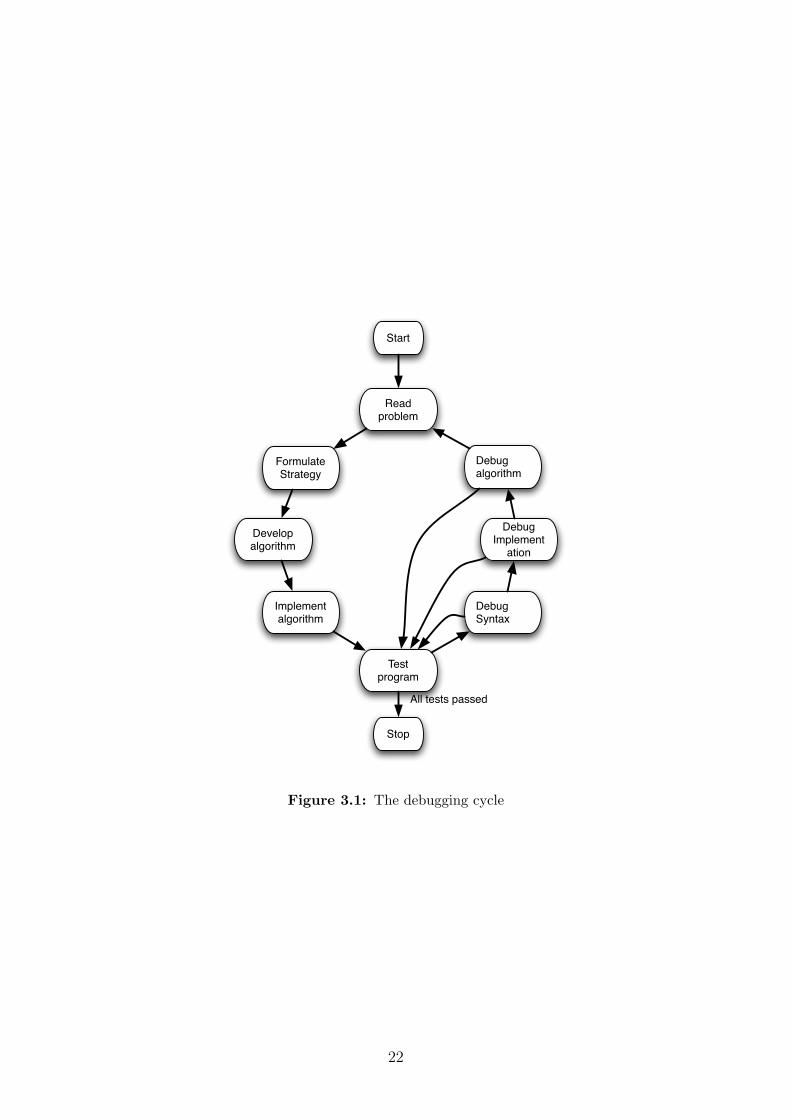
The cycle of development is shown in figure ??.

3.2 Types of errors

3.2.1 Syntax errors

The syntax of a language are the basic rules that define which words are allowed, whatsequence of words is allowed and which punctuation marks are required. A human reader

21

Read problem

Formulate Strategy

Debug Implement

ation

Debug algorithm

Develop algorithm

Implement algorithm

Debug Syntax

Start

Stop

Test program

All tests passed

Figure 3.1: The debugging cycle

22

can usually determine the semantics or meaning of a sentence even when the syntax isincorrect. “Me dog is want food” is syntactically incorrect, but the meaning is (relatively)clear. Unfortunately, computers lack the context and experience to accurately determinethe meaning of an expression if the syntax laid out by the language you are using is notfollowed very closely. This means that Octave does a preliminary syntax check beforeeven attempting to execute any function you have written.

The visible effect of this is that syntax errors are always the first hurdle to getting yourfunction to work. Octave syntax is relatively simple and following the examples shouldallow you to steer clear of most problems. Things to watch out for when debugging syntaxerrors are:

• make sure all operators and functions have the correct number of arguments (a *

needs an argument on both sides, mod needs two arguments separated by a comma)

• Octave regards the end of a line as the end of your statement. If you mean for yourstatement to span lines, use the ... operator, which indicates to Octave that theline should be continued

• certain structures like if require a closing statement, which in Octave is alwaysend. Octave will only complain after having searched through the entire file for thecorrect end, so be sure to search well for this one.

3.2.2 Semantic errors

When all the syntax has been sorted out, Octave will attempt to run your function. Atthis point the meaning of your program becomes important. Clearly, a sentence like“computers swim very well” is syntactically correct, but the sentence does not makesense. Again, the computer cannot attempt to make sense of what we have written, evenif the syntax is correct. It is up to you to say what you mean clearly and rephrase untilthe computer interprets it the way you want it to.

3.3 Pre-emptive maintainence

There are many things that one can do to stop problems from occurring in the first place,but most of the pre-emptive action that can be taken is to enable the programmer to findproblems before they happen. To do this effectively, you need to make the program codeeasy to read. The clearer your program is, the less chance there is of a mistake slippingin.

3.3.1 Comment

Comments in Octave are introduced using the % character. All the remaining characterson the line will be treated as though they were not there. Comments help to clarify whatyou are doing in words that you can understand.

1 % FACT determine the f a c t o r i a l2 % FACT(N) c a l c u l a t e s the f a c t o r i a l us ing a r e cu r s i v e t echn ique3 %4 % See a l s o f a c t o r i a l5 %

23

6 % NOTE: Do not use f o r N > 1007

8 % Author : Carl Sandrock9

10 function r = f a c t (N)11 i f N == 012 r = 1 ;13 else % recurse f o r prev ious terms14 r = N∗ f a c t (N − 1) ;15 end

A handy Octave feature is that typing help fact will show the first block of commentsin the fact function, giving you the same type of information that you would find fromany built-in Octave command. It even builds hyperlinks to the factorial function’s helpthat we referenced using “See also”.

3.3.2 Indent

You may have noticed that the code examples for the conditional statements in chapter 2and the fact function above used a simple convention for the display of nested structures.The nested parts where indented a certain distance to the right. This makes followingthe structure of a complicated piece of code easier, leading to less mistakes.

The Octave editor will usually do indentation automatically, but every so often (usu-ally after intense editing) your indentation may become disrupted. can automaticallyindent your code when you select a piece of code and select “Text—Smart indent” fromthe menu.

3.3.3 Space

Using proper spacing can improve the legibility of your code. Comparer=1+N/3-f(a,b^3) tor = 1 + N/3 - f(a, b^3).

A good rule is to use spaces on both sides of +, -, =, |, >, <, <=, >= and ==, and touse a single space after a comma as used in writing.

3.3.4 Parenthesise

If the precedence in an expression is unclear, use parenthesis liberally to group expressionsfor evaluation. Make sure you understand the precedence of the most often used operators,found in Table 2.2 of Hahn.

3.3.5 Aim for readability

The goal should always be to keep your readable. If there are confusing bits in yourprogram, give them names by defining more functions.

For example,

1 i f mod(N, 2) == 02 % do something3 else

24

4 % do something e l s e5 end

could be made more readable by using a function to show what the formula in line 1 does(and adding some comments)

1 i f i s ev en (N, 2)2 % do somethinng3 else % N i s odd4 % do something e l s e5 end

3.3.6 Keep functions short

Octave is an expressive language, so you should be able to express most problems in ashort, intuitive way. If you find yourself using more than about 20 lines of code, you areprobably in need of more functions.

3.4 Tools and tricks

3.4.1 Octave

One important way to debug functions is by displaying the values of variables while theprogram executes by removing the trailing semicolons after assignments. In later chaptersyou will see how to produce better looking output, but for now, let’s return to our factfunction. Edit fact.m so that line 5 does not end with a semicolon. Now, when you runit, you should see something like the following:

octave> fact(5)

r = 1

r = 2

r = 6

r = 24

r = 120

ans = 120

Notice how Octave shows the assignment each time it happens.The most important thing to remember when a function is not running as it is sup-

posed to, is to read. You must read both the error messages Octave prints out and yourcode.

3.4.2 Excel

The greatest strength of spreadsheeting – that of hiding the formulae from the user andfocusing on the results – turns out to be its greatest weakness as well. Although a workingspreadsheet is easy to use and can be made to please the eye, the opacity of spreadsheetcells displaying values can become a problem.

Excel handles this in two ways: by allowing us to reveal the formulae in a sheet andproviding ways of finding the dependence of one cell on another graphicalle. The hotkey

25

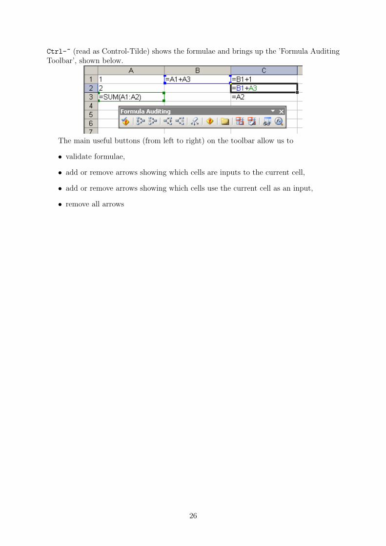
Ctrl-~ (read as Control-Tilde) shows the formulae and brings up the ’Formula AuditingToolbar’, shown below.

The main useful buttons (from left to right) on the toolbar allow us to

• validate formulae,

• add or remove arrows showing which cells are inputs to the current cell,

• add or remove arrows showing which cells use the current cell as an input,

• remove all arrows

26

Chapter 4

Variables and types

On two occasions I have been asked [by members of Parliament], ’Pray, Mr. Babbage,if you put into the machine wrong figures, will the right answers come out?’ I am notable rightly to apprehend the kind of confusion of ideas that could provoke such a question.

Charles Babbage (1791 – 1871)

After completing this chapter you should be able to

• Describe and understand the use of variables

• Create matrices of numbers

• Know the difference between numbers and strings

• Apply functions to numbers and strings

• Create cell arrays

• Understand the difference between matrices and cell arrays

• Import data from files

4.1 Introduction

If you have mastered logic functions, creation of functions, conditionals and recursion,you can provably solve any computable problem. Unfortunately the proof of the existenceof a solution says nothing about the practicality of a solution.

This chapter introduces two basic concepts: variables as containers for values andtypes of values. Unlike logic or conditional execution, data structures more advancedthan simple numbers (or 1 and 0 for that matter) are not strictly required for the solutionof a problem. They help to make the solution easier to understand and to implement inaddition to saving memory and processor time.

4.2 Variables

4.2.1 Scalar variables

So far, all the functions that we have created have only included references to their inputsand outputs and other functions. You may already have started using other variables to

27

simplify your programs, without knowing exactly how they work.Octave supplies us with space to store intermedate results. It allows us to place values

in variables, which can be considered as labelled containers. The = or assignment op-erator places the result of the expression on the right hand side (RHS) in the variable(s)on the left hand side.

Note that the RHS is completely evaluated before being stored in the variable, so thatthe following Octave session may happen (in the command window):

octave> a = 1;

octave> b = 2;

octave> x = a + b;

octave> a = 3;

octave> x

x = 3

In the above code section, notice how I used the semicolon (;) to suppress output (stopOctave from showing me each result). Also notice how the value of x was unchanged whenwe changed a. This is because the whole expression a+b was evaluated before storing theresult in x. Octave has no memory of how a value is calculated, only storing the resultof the calculation. To remember this, it is helpful to imagine an arrow from right to leftin all assignments (x ← a+b).

Also notice how the sequence in which we typed the instructions above is very im-portant. Up to now, it is would have been very unlikely for you to make a sequencingerror, as all our functions have been built to avoid this problem. When assigning valuesto variables, it is clear from the example above that the sequence in which we do things isvery important. The golden rule is that Octave evaluates every file from top to bottom.

4.2.2 Scope

Variables assigned in the command window are held in a space known as the workspace.This is the space that we viewed using the workspace viewer when doing debugging. Everytime a function is called, the variables created in that function occupy a separate spacetogether with the input arguments of the function. Note that the space is created witheach call or evaluation of the function, not the function itself, so one function can havemany spaces. When the function terminates, the values in variables that are indicatedas outputs in the function are returned and all the variables in the space are deleted.

The above idea is known as variable scope. The scope of a variable is the area whereit can be “seen” by calling functions.

To understand variable scope, it is useful to think of variables as labelled boxes. Eachtime we assign a value to a variable we are “putting it into a box”. When we use a variablename, we are making a copy of the value in a box. In the description of a sequence ofevents below, the scope is indicated by a box as well.

Let’s say we have defined this function:

1 function z = add (a , b)2 z = a + b3 end

28

First, we create three variables x, y, and z

octave> x = 1;

octave> y = 3;

octave> z = x + y;

Workspacex 1

y 3

z 4

Then, we replace the contents of x with a 9

octave> x = 9;

Notice that z still contains the same value

Workspacex 9

y 3

z 4

Calling the function creates a new scope with two newvariables a and b

octave> y = add(x, z);

Workspacex 9

y 3

z 4

adda 9

b 4

The line z=a+b inside the add function creates a newz variable in the “add” scope. Note that the z on theworkspace still contains the same value.

Workspacex 9

y 3

z 4

adda 9

b 4

z 13

When the function terminates, the “add” scope isdeleted along with all the variables inside it. Becausethe function definition defined z as an output vari-able, the value in z is returned as the result of thefunction and y is changed in the Workspace scope.

Workspacex 9

y 13

z 4

4.2.3 Vectors and matrices

Creating matricesManual§4.1So far, we have been working only with scalar values. If you look at the workspace

browser or use the Octave command whos, you will notice that all the variables we havedefined have a size of 1× 1. This is because Octave was developed with matrices in mindfrom the beginning. To create vectors you use square brackets ([ and ]) to indicate thestart and end of a vector definition and elements can be separated using commas or (morecommonly) spaces. To create matrices, you separate rows with semicolons.

octave> a = [1 2 3]

a =

1 2 3

octave> b = [1 2; 3 4]

b =

1 2

3 4Manual§16.4It is often easier to use one of the built-in utility matrices to create matrices. The

important functions eye, ones, zeros and rand all accept a number of rows and columnsas arguments and return an identity matrix, a matrix consisting of ones or zeros anda random matrix respectively. If only one dimension is specified, a square matrix isreturned.

octave> eye(4)

29

ans =

1 0 0 0

0 1 0 0

0 0 1 0

0 0 0 1

octave> ones(2, 4)

ans =

1 1 1 1

1 1 1 1

octave> zeros(1, 10)

ans =

0 0 0 0 0 0 0 0 0 0

octave> rand(3, 2)

ans =

0.69995 0.82151

0.16199 0.49675

0.37963 0.43924

4.2.4 Concatenation

One element that is not immediately obvious is that other vectors can be used in thecreation of vectors and matrices, in a process called concatenation, as shown below:

octave> b = [a 4 5]

b =

1 2 3 4 5

octave> C = [a; a; a]

C =

1 2 3

1 2 3

1 2 3

We say that C contains three copies of the contents of a concatenated vertically and thatb contains the vector [4 5] concatenated to the contents of a. This behaviour will comein really handy in functions.

Even when we are building a vector like [1 2 3], we are using the concatenationoperator to put three scalar values together in a vector.

4.2.5 RangesManual§4.2The colon (:) operator in Octave can be used to create uniformly spaced vectors. The

basic form for this structure is start:end, creating a vector going from start to end inincrements of 1.

octave> 1:10

ans =

1 2 3 4 5 6 7 8 9 10

octave> 0.1:5

ans =

0.10000 1.10000 2.10000 3.10000 4.10000

30

Alternatively, you can use start:increment:end, which uses the specified incrementrather than 1, as shown below:

octave> 0:.1:0.5

ans =

0.00000 0.10000 0.20000 0.30000 0.40000 0.50000

octave> 0:10:50

ans =

0 10 20 30 40 50

An interesting feature is that an empty matrix is produced when end¡start. Thismeans that a negative increment must be specified when generating numbers backwardas follows:

octave> 10:1

ans = [](1x0)

octave> 10:-1:1

ans =

10 9 8 7 6 5 4 3 2 1

SubscriptingManual§8.1In Octave, the concept of indexing or subscripting as expressed by a vector notation

like xi, giving the ith element of x is expressed by brackets as in x(i). For multipleindices, like the matrix notation Aij, we would use A(i, j). Indexing works on bothsides of an assignment, so we can assign values to items inside an existing matrix as wellas getting the values out, like the following:

octave> A = [1 2 3; 4 5 6]

A =

1 2 3

4 5 6

octave> A(2, 1)

ans = 4

octave> A(2, 1) = 0

A =

1 2 3

0 5 6

Note: Octave supplies an automatic value for end in matrix expressions, representingthe last index of a vector. This means that if k = [11 12 13 14], k(end) will be 14.

It is also possible to use vectors as subscripts as in the following examples:

octave> A = [1 2 3; 4 5 6]

A =

1 2 3

4 5 6

octave> A(1, [2 3])

ans =

31

2 3

octave> A([1 2], 1)

ans =

1

4

octave> A([1 2], [2 3])

ans =

2 3

5 6

4.2.6 Application

Fibonacci again

Let’s see an application of this new information. Let’s say we wanted to modify the fib

function we wrote a while back to output the first N fibonacci numbers instead of only theN th one. Conceptually, we can see that if we have a partial list of N −1 numbers, we canfind the last one by adding the previous two. In Octave code, (with the previous N − 1numbers in the vector p) this concept is expressed as r = [p, p(end-1) + p(end)],which is read as “the result of the function is the concatenation of the previous N − 1terms with the sum of the last two”.

The function is shown here:

7 function r = f ib vec (N)8 i f N == 19 r = 1 ;

10 e l s e i f N == 211 r = [ 1 1 ] ;12 else13 p = f ib vec (N−1) ;14 r = [ p , p(end−1)+p(end) ] ;15 end

Vectorising operations

The use of vectors in Octave is highly encouraged. Using vectors and functions thatoperate on them we can determine many of the answers to questions we have previouslyanswered without creating functions at all. For instance, let’s look at the series productagain:

c =N∏

i=1

a/N

Manual§17.4We can find this answer easily by using vector notation as follows:

octave> N = 30;

octave> a = 10;

octave> prod(a./(1:N))

ans = 0.0038

Here is another function using vectors to find the smallest element in a vector:

32

12 function m = findmin (v )13 i f length ( v ) == 114 m = v ;15 e l s e i f length ( v ) == 216 i f v (1) < v (2)17 m = v (1) ;18 else19 m = v (2) ;20 end21 else22 m = findmin ( [ v (1 ) f indmin (v ( 2 :end) ) ] ) ;23 end

This function works by making the observation that the minimum is always the firstelement unless there is a smaller element in the rest of the vector. Follow the logic of thisfunction closely, especially noting the use of the length function.

Sorting

There are many algorithms for sorting lists. One of the simpler ones is called selectionsorting. This is probably the method you would use to sort a hand of cards. The idea isthat you start with a stack of unsorted cards and move the cards one by one to a secondstack, taking care to place it in the correct position. The following function shows onepossible implementation of a selection sorting procedure.

1 function so r t ed = s e l s o r t ( unsorted , workspace )2 i f isempty ( unsorted )3 so r t ed = workspace ;4 else5 f i r s t i t e m = unsorted (1 ) ;6 unsorted = unsorted ( 2 :end) ;7 workspace = i n s e r t ( f i r s t i t em , workspace ) ;8 so r t ed = s e l s o r t ( unsorted , workspace ) ;9 end

10

11 function new l i s t = i n s e r t ( item , l i s t )12 % assume the l i s t i s s o r t ed a l r eady13 i f isempty ( l i s t )14 new l i s t = item ;15 e l s e i f item < l i s t (1 )16 new l i s t = [ item l i s t ] ;17 else18 new l i s t = [ l i s t (1 ) i n s e r t ( item , l i s t ( 2 :end) ) ] ;19 end

One calls this function with a list to sort and an empty vector for the workspace, forexample:

octave> selsort([3 2 1 4 3], [])

ans =

1 2 3 3 4

33

Here is how this all works: If there are no unsorted items, we are done and theworkspace constains all the sorted items (lines 2-3). If there are some items, we take thefirst one out of the unsorted ‘heap’ and insert it into the workspace (lines 5-7). Then, werepeat this process with a smaller heap of items to sort and a larger, sorted, workspace.

A key part of this algorithm is the insert function which we define in the same file.This puts one item in the correct place in an already sorted list. Clearly if the list isempty, we just have the one item we wanted to insert as output (lines 13-14). Otherwise,if our item is less than the first item of the list, we return a new list with the item in thefront (lines 15-16). If that didn’t work, we try to put the item into the rest of the list(lines 17-18).

4.2.7 Exploration

These problems are not for marks, but give you some interesting ideas to follow up on.

1. Determine the sum of all the odd numbers between 3 and 1503, inclusive using oneOctave command

2. Compare fib_vec.m to fib.m. Try running them to find the 25th Fibonacci num-ber. Why is fib.m so much slower than fib_vec.m?

3. What do the following vector functions do? mean, sum, min, max, prod, horzcat,vertcat

4. What is the difference between \ and / in Octave? Check the effect using matrices

5. What is the difference between the “normal” operators -+*/\ and the “dotted”operators with a . in front of them?

4.3 Types

4.3.1 Concept

Up to now, we have been working with numbers in our programs. In the previous sectionyou saw that we could form groups of numbers by concatenating them into vectors andmatrices. Octave can do more than just numbers – there are several types of values.

In Octave values have types, but variables do not. The type of a variable can changemany times in a program, depending on what type of data is stored in that variable atthe time. Octave calls the type of a variable its class. You can see what class a variable isby executing the command whos. Each of the currently defined variables is listed towardthe end of the output. You will see a class column on the right hand side.

4.3.2 Complex values

Octave can handle complex as well as real values. The variables i and j are normallyassigned to be equal to

√−1. In the Octave command window, we can see the effect:

octave> i^2

ans = -1

octave> sqrt(-4)

34

ans = 0 + 2.0000i

octave> a = 4 + 3i

a = 4.0000 + 3.0000i

4.3.3 StringsManual§5Numbers seem to come naturally to computers, and we have seen a few ways in which

they can be represented. But we are familiar with other uses for computers that do notseem to be directly related to numbers. The document that you are reading seems to bemade up of characters and words. In computer terminology, such sequences of charactersare called strings.

The computer can only work with ones and zeros, so there have to be ways to translatefrom ones and zeros to characters and words. One common convention is to set up a tableof characters corresponding to numbers. One common table is the American StandardCode for Information Interchange (ASCII) table. This maps 7 bit values (256 differentones in all) to useful characters.

Octave handles strings as vectors of characters and uses 8 bit characters, starting withthose defined in the ASCII table, extended by new characters. The exact contents of thetable is not important (and, in fact varies between different types of computers), but canbe obtained from many sources, including http://en.wikipedia.org/wiki/ASCII.

Octave uses single quotation marks1 to indicate string literals (values that must beinterpreted directly). Consider the following Octave session:

octave> ’my name is’

ans =my name is

octave> t = ’pete’

t = pete

octave> t(2)

ans = e

We say that the ’my name is’ in the above example is a string literal, while t wouldbe a string variable after assignment. In Octave’s terminology, t is known as a characterarray or character vector. This explains why it is possible to display the second elementof the array using normal vector indexing.

Program output

Using strings makes it possible to communicate with the user using more than just num-bers. To display a string value on the screen, the disp function can be used as follows:

octave> disp(’Hello’)

Hello

octave> disp(t)

pete

Note that disp simply displays an array, and as such can be used for numeric valuesas well. It is however, usually used to inform the user of a program of the status orintermediate results of a program.

1Double quotes may also be used, but this is not compatible with Matlab

35

Concatenation

It is often required to combine the values of different variables to achieve a user-friendlyoutput. The normal concatenation operator [] can be used to concatenate strings, asfollows:

octave> greeting = ’hello ’

greeting = hello

octave> myname = ’pete’

myname = pete

octave> [greeting myname]

ans = hello pete

Notice how greeting was assigned a value that included a trailing space, so thatwhen myname was concatenated to it, it would present a readable string.

It is helpful to remember that each of the characters in the string is stored as a number,so the operations on strings and numeric vectors operate in a consistent manner.

Conversion

What happens when we attempt to mix types? What if we tried to add 1 to the string“pete”?

octave> ’pete’ + 1

ans =

113 102 117 102

Octave tries to interpret this statement in a way that will not result in an error, and endsup adding 1 to each of the numbers in the string “pete”. Remember that each charactersis actually stored as a number. The fact that an “e” looks like an “e” is all up to thetable the computer is using, so we just get the next number on in the table as a result.

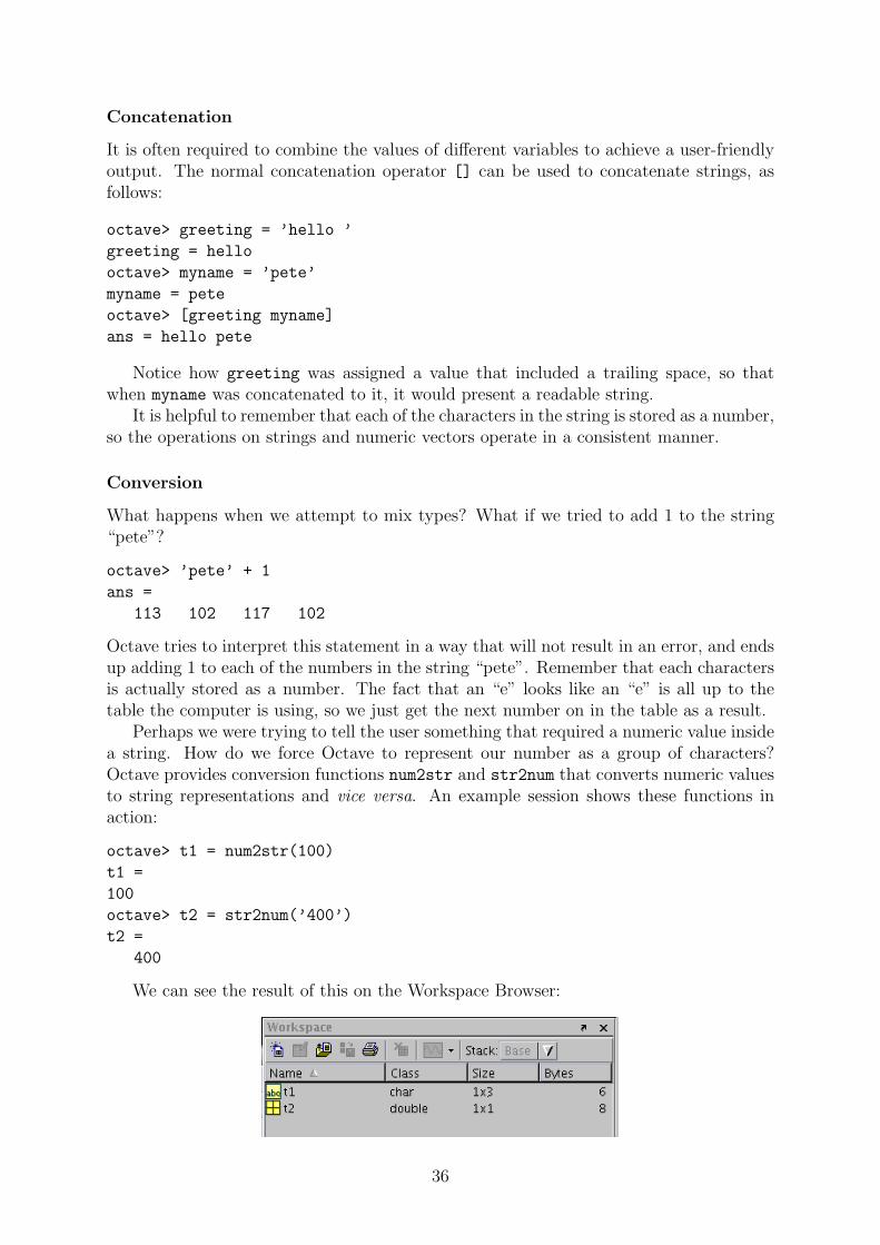
Perhaps we were trying to tell the user something that required a numeric value insidea string. How do we force Octave to represent our number as a group of characters?Octave provides conversion functions num2str and str2num that converts numeric valuesto string representations and vice versa. An example session shows these functions inaction:

octave> t1 = num2str(100)

t1 =

100

octave> t2 = str2num(’400’)

t2 =

400

We can see the result of this on the Workspace Browser:

36

Comparison

Because strings are stored as vectors of characters, the normal == operator does not workquite as one would expect. Conceptually, we can imagine strings being equal when alltheir characters are equal, but what if they have differing numbers of characters?

Octave’s solution to this problem is the strcmp function, which returns 1 if its twoarguments are the same string and 0 if they differ.

octave> a = ’this’

a = this

octave> b = ’isatest’

b = isatest

octave> a == b

error: mx_el_eq: nonconformant arguments (op1 is 1x4, op2 is 1x7)

error: evaluating binary operator ‘==’ near line 54, column 3

octave> strcmp(a, b)

ans = 0

octave> strcmp(a, a)

ans = 1

4.3.4 Function handles

You have come across the function handle operator before. The function handle that thefunction handle operator returns is also a different type. We can see this by executingf = @sin and observing the class reported for f in the output of whos. It is reported as“function handle”.

4.4 Cell arrays

4.4.1 The problemManual§6.2Octave allows us to place simple values in vectors and matrices to group them together.

We can see that a matrix of values can be interpreted as a “list of lists”, in other words,one can think of each row of the matrix representing a collection of values.

For instance, if we have the marks for 3 students in 4 subjects, we could choose tostore the marks in three rows of a matrix as follows:

octave> stud1 = [75 50 54 45];

octave> stud2 = [90 50 56 40];

octave> stud3 = [80 50 60 70];

octave> marks = [stud1; stud2; stud3]

marks =

75 50 54 45

90 50 56 40

80 50 60 70

A function that will calculate the average mark for each student could look like this:

1 function a = markaverage (marks )2 i f isempty (marks )

37

3 a = [ ] ;4 else5 a = [mean(marks (1 , : ) ) ; markaverage (marks ( 2 :end , : ) ) ] ;6 end

However, if not all students are enrolled for the same number of subjects, it becomesdifficult to use a matrix, as we can only concatenate items with matching dimensions.

Let’s say there is a fourth student who only has 3 subjects.

octave> stud4 = [80 58 54];

octave> marks = [stud1; stud2; stud3; stud4]

??? Error using ==> vertcat

CAT arguments dimensions are not consistent.

We see that we cannot concatenate the fourth student as that would result in a rowwith less columns than the rest!

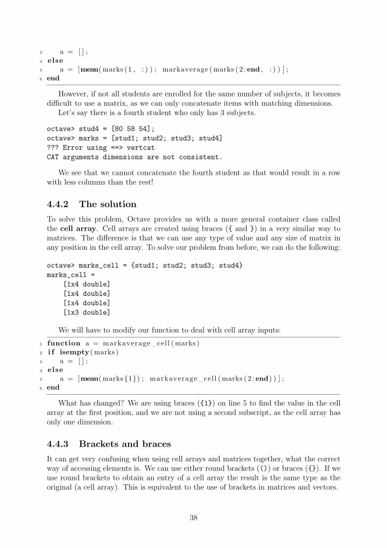
4.4.2 The solution

To solve this problem, Octave provides us with a more general container class calledthe cell array. Cell arrays are created using braces ({ and }) in a very similar way tomatrices. The difference is that we can use any type of value and any size of matrix inany position in the cell array. To solve our problem from before, we can do the following:

octave> marks_cell = {stud1; stud2; stud3; stud4}

marks_cell =

[1x4 double]

[1x4 double]

[1x4 double]

[1x3 double]

We will have to modify our function to deal with cell array inputs:

1 function a = markaverage ce l l (marks )2 i f isempty (marks )3 a = [ ] ;4 else5 a = [mean(marks {1}) ; markaverage ce l l (marks ( 2 :end) ) ] ;6 end

What has changed? We are using braces ({1}) on line 5 to find the value in the cellarray at the first position, and we are not using a second subscript, as the cell array hasonly one dimension.

4.4.3 Brackets and braces

It can get very confusing when using cell arrays and matrices together, what the correctway of accessing elements is. We can use either round brackets (()) or braces ({}). If weuse round brackets to obtain an entry of a cell array the result is the same type as theoriginal (a cell array). This is equivalent to the use of brackets in matrices and vectors.

38

[ ]

( )

Figure 4.1: The use of brackets when creating and referencing ordinary arrays (matrices). Use[] to construct matrices, () to index.

Cell arrays can be seen as similarly shaped containers with differently shaped contents.If we only want the information stored in the container, curly brackets should be used.The use of brackets when creating and referencing ordinary arrays is shown in figure 4.1

The same procedure is shown for cell arrays in figure 4.2.

( )

{}

{}

{}

Figure 4.2: The use of braces when creating and referencing cell arrays. Use {} to construct,() to subscript with cell return value, {} to subscript with inside return value

4.4.4 Cell arrays and strings

Because Octave stores strings as vectors of characters, it is possible to form matrices ofcharacters by concatenating strings. There is a catch – the strings all have to be the samelength. The cell array can solve this problem as well. Let’s say we wanted to modify ourmarks function to display the average marks next to a student’s name rather than returnthem. Or displaying function could look like this:

1 function markaverage disp (names , marks )2 i f ˜isempty (marks )3 disp ( [ names{1} ’ - ’ num2str(mean(marks {1}) ) ] ) ;4 markaverage disp ( names ( 2 :end) , marks ( 2 :end) ) ;5 end

39

octave> marks_cell = {stud1; stud2; stud3; stud4};

octave> names = {’Jack’, ’Jill’, ’Jane’, ’John’};

octave> markaverage_disp(names, marks_cell)

Jack - 56

Jill - 59

Jane - 65

John - 64

4.5 Dealing with data

4.5.1 Load and saveHahn§16.1Octave provides several ways of accessing files. The most common ones you will be

using are the load and save functions. Without arguments, save will save the currentworkspace in a file called matlab.mat. If you exit Octave and execute the load commandin the same directory, your variables will reappear. You can save to a specific filenameusing save(filename), where filename is a string. You can use the same idea by sayingload(filename).

Be sure to read Hahn section 16.2 for more detail.

4.5.2 Importing dataHahn§16.2Other data can usually be imported into Octave using the “File—Import data—” menu

option. The import wizard will guide you through this process. If the file you areimporting contains text mixed with numeric values, Octave will import the text into acell array and the numbers into a matrix.

4.6 Assignments

1. Write a function oddsum that accepts two numbers and returns the sum of theodd numbers between them. Make sure it works regardless of the numeric order ofthe two numbers and regardless of whether the numbers are odd or not. Examplesession:

octave> oddsum(3, 3)

ans =

3

octave> oddsum(3, 5)

ans =

8

octave> oddsum(302, 5)

ans =

22797

2. Write a function called givecoin that will accept a vector of coin values in descend-ing order and an amount and return the largest coin value less than the amount.Example session:

40

octave> sacoins = [100 50 20 10 5];

octave> givecoin(sacoins, 23)

ans =

20

octave> givecoin(sacoins, 200)

ans =

100

octave> givecoin(sacoins, 2)

ans =

[]

3. Use the givecoin function to write a function called givechange that accepts avector of coin values and an amount and returns a vector of coins given as change.You may assume that you can simply give the largest coin possible for the amount,then subtract that coin value from the amount and repeat the process until no morecoins can be given.

Example session:

octave> sacoins = [100 50 20 10 5];

octave> givechange(sacoins, 233)

ans =

[100 100 20 10]

octave> givechange(sacoins, 5)

ans =

5

octave> givechange(sacoins, 3)

ans =

[]

4. Write a function called pointonline that will accept three inputs and one output.The first two inputs (p1 and p2) are both vectors containing the x and y coor-dinates of points on a line while the third input (x) is a scalar value giving an xvalue on this line. The function must calculate the corresponding y value as output.

��

��

��

��

��

��

��

v p1

v p2

v(x, y)

With p1 = [x1y1] and p2 = [x2y2],

y − y1

x− x1

=y2 − y1

x2 − x1

so

y = y1 + (x− x1)×y2 − y1

x2 − x1

Sample output:

octave> pointonline([0 0], [1 1], 0.5)

ans =

41

0.5000

octave> pointonline([1 1], [0 0], 0.5)

ans =

0.5000

octave> pointonline([1 1], [2 2], 1.5)

ans =

1.5000

octave> pointonline([1 2], [2 3], 1.5)

ans =

2.5000

5. Write a function called interpolate that will accept three arguments, known_x,known_y and x. known_x and known_y represent a table of values as shown be-low, and x represents the x value to find the corresponding y value of using linearinterpolation.

known_x known_y

1 32 103 204 206 15

If x is 5, we know that y lies on the line defined bythe points (4, 20) and (6, 15) and we can use thepointonline function to do the interpolation for us(finding y = 17.5). interpolate will therefore mainlyfind the rows to interpolate on. You may assume thatknown_x is strictly increasing and that x is betweenthe smallest and largest values in known_x.

octave> known_x = [1 2 3 4 6];

octave> known_y = [3 10 20 20 15];

octave> interpolate(known_x, known_y, 5)

ans =

17.5000

octave> interpolate(known_x, known_y, 3.2)

ans =

20

6. Write a function called christmas that will accept an integer argument N anddisplay stars in the shape of a Christmas tree N characters high as follows :

octave> christmas(3)

*

***

|

octave> christmas(6)

*

***

*****

*******

42

*********

|

Note that the stem (at the bottom) should always be one character.

7. A palindrome is a phrase or number that is the same written from left to right orright to left. Usually, punctuation and spaces do not count, so some interestingpalindromes are:

• laminar animal

• Live not on evil

• A man, a plan, a canal – Panama!

Write a function called ispal that will return 1 if its argument is a palindrome and0 if it is not (you do not have to remove spaces and punctuation).

octave> ispal(’amanaplanacanalpanama’)

ans =

1

octave> ispal(’notapalindrome’)

ans =

0

8. Palindromic numbers have some interesting properties. Starting with a numberlike 12, we find that if we add the number to its reversed number (21), we get apalindrome (33). For some numbers, we need to repeat the process a few times.For instance, starting with 59, we find the following sequence:

(a) 59 + 95 = 154

(b) 154 + 451 = 605

(c) 605 + 506 = 1111, which is a palindrome.

Write a function that will determine how many steps (iterations) are required beforea number becomes a palindrome using this procedure. Your function must receiveone input, the seed number and return one output, the number of iterations. Noadditional output must be generated.

Hint: Use the ispal function after converting to a string to check if a number is apalindrome.

Sample output:

octave> findpal(11)

ans =

1

octave> findpal(61)

ans =

2

43

octave> findpal(651)

ans =

4

octave> findpal(151)

ans =

1

octave> findpal(153)

ans =

3

Don’t try to run findpal on 196 – this number is not known to have a palindromicsequence, even though several million iterations have been done!

9. Write a function called divisors that returns a vector of the divisors of its input(all the integers less than or equal to a that divide into a with no remainder a,including a).

Sample output:

octave> divisors(1)

ans =

1

octave> divisors(4)

ans =

4 2 1

octave> divisors(6)

ans =

6 3 2 1

octave> divisors(56)

ans =

56 28 14 8 7 4 2 1

10. Write a function divisors_vec that returns a cell array containing the divisors ofeach of the elements of its input, which is a vector. Use the divisors function youhave just written.

Example output:

octave> t = divisors_vec([56 13 23])

t =

[1x8 double] [1x2 double] [1x2 double]

octave> t{1}

ans =

56 28 14 8 7 4 2 1

44

octave> t{2}

ans =

13 1

octave> t{3}

ans =

23 1

45

Chapter 5

Loops

A small error in the beginning can lead to great ones in the end.

St. Thomas Aquinas (1225–1274) paraphrasing Aristotle (322–384 BCE)

After completing this chapter you should be able to

• Distinguish between functional and imperative approaches to programming

• Understand and use deterministic and non-deterministic loops

• Distinguish between the loop types

• Decide between different repitition techniques

• Identify the roles of variables in loops

5.1 Imperative algorithms

Recursion is a powerful way of expressing repeated operations, but can become difficultto understand if one is not careful. Octave provides other ways of handling repetitivetasks called loops.

So far, we have expressed algorithms as networks of functions. This is called thefunctional approach to programming. In this approach, we do not need to use temporaryvariables to store intermediate results but instead use function calls and recursion tocreate new versions of the inputs and output of functions. In technical terms, we areusing the function inputs and outputs to store the state of the program.

A contrasting view of algorithms is to write them down as a series of steps. This iscalled the imperative view. In this view, we need variables to store the state of theprogram. For instance, to sum the elements of a vector, we need a variable to store therunning total as we step through the elements. Octave encourages a mix of functionaland imperative techniques.

5.2 Types of iteration

Consider the following problems:

46

1. Determine the sum of all odd integers between a and b, assuming a and b are oddand a < b

2. Determine the number of coins to be given as change given a vector of coin valuesc and an amount a

In the first case, it is possible to determine exactly how many odd integers there are –there will be b−a

2+1. It is also possible to enumerate or write down all of the candidate

numbers. This type of repeating task is called deterministic. In the second case, it isnot easy to determine how many coins will be given as change without actually goingthrough the process of giving coins until all the change is given. This type of repeatingtask is called non-deterministic.

5.2.1 Deterministic loopsManual§10.5Octave provides one generic form of loop for situations where it is known beforehand how

many times a loop is to run. The syntax for this loop is shown below:

-- ‘for’ 〈variable〉 ‘=’ 〈matrix 〉 〈block〉 ‘end’ -�

When Octave encounters a for statement, it evaluates the statements between forand end exactly Nc times, where Nc is the number of columns in matrix. Before eachexecution, the next column of matrix is stored in variable, which is then accessible tothe statements in the loop.

As an example, consider the first off the problems in section 5.2. One solution to thisproblem using a for loop is shown here:

1 function s = oddsumfor ( a , b)2 s = 0 ;3 for n = a : 2 : b4 s = s + n ;5 end

Notice how the term a:2:b is evaluated first, yielding a vector with the elements thatwe want to sum. Each column of this vector is a single element, which is assigned to n

for each run of the loop.An interesting edge case occurs when the matrix has no columns at all, which only

happens when the matrix is the empty matrix ([]). As there are no columns, the loopis not evaluated at all. Try running the oddsumfor function with a < b. Why does theloop not run?

A common misconception about Octave’s for loop is that the construction of thematrix is a part of the syntax. This is not true, but can be misleading if all the loopsone encounters are of the type in oddsumfor. See if you can see how the next example(which is a reworking of a previous example) works:

1 function c o i n t og i v e = g iveco in f o r ( co ins , amount )2 c o i n t og i v e = [ ] ;3 for t h i s c o i n = co in s (end :−1:1)4 i f t h i s c o i n <= amount5 c o i n t og i v e = th i s c o i n ;6 end7 end

47

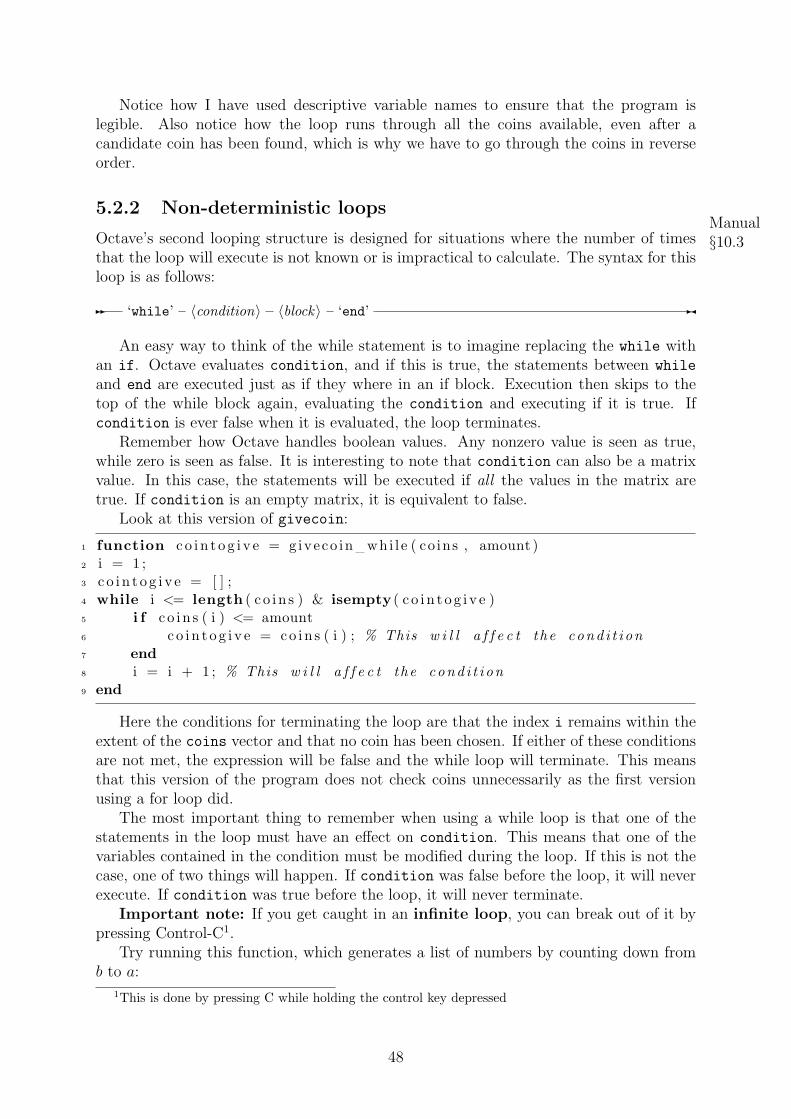
Notice how I have used descriptive variable names to ensure that the program islegible. Also notice how the loop runs through all the coins available, even after acandidate coin has been found, which is why we have to go through the coins in reverseorder.

5.2.2 Non-deterministic loopsManual§10.3Octave’s second looping structure is designed for situations where the number of times

that the loop will execute is not known or is impractical to calculate. The syntax for thisloop is as follows:

-- ‘while’ 〈condition〉 〈block〉 ‘end’ -�

An easy way to think of the while statement is to imagine replacing the while withan if. Octave evaluates condition, and if this is true, the statements between while

and end are executed just as if they where in an if block. Execution then skips to thetop of the while block again, evaluating the condition and executing if it is true. Ifcondition is ever false when it is evaluated, the loop terminates.

Remember how Octave handles boolean values. Any nonzero value is seen as true,while zero is seen as false. It is interesting to note that condition can also be a matrixvalue. In this case, the statements will be executed if all the values in the matrix aretrue. If condition is an empty matrix, it is equivalent to false.

Look at this version of givecoin:

1 function c o i n t og i v e = giveco in whi l e ( co ins , amount )2 i = 1 ;3 c o i n t og i v e = [ ] ;4 while i <= length ( c o in s ) & isempty ( c o i n t og i v e )5 i f co in s ( i ) <= amount6 c o i n t og i v e = co in s ( i ) ; % This w i l l a f f e c t the cond i t i on7 end8 i = i + 1 ; % This w i l l a f f e c t the cond i t i on9 end

Here the conditions for terminating the loop are that the index i remains within theextent of the coins vector and that no coin has been chosen. If either of these conditionsare not met, the expression will be false and the while loop will terminate. This meansthat this version of the program does not check coins unnecessarily as the first versionusing a for loop did.

The most important thing to remember when using a while loop is that one of thestatements in the loop must have an effect on condition. This means that one of thevariables contained in the condition must be modified during the loop. If this is not thecase, one of two things will happen. If condition was false before the loop, it will neverexecute. If condition was true before the loop, it will never terminate.

Important note: If you get caught in an infinite loop, you can break out of it bypressing Control-C1.

Try running this function, which generates a list of numbers by counting down fromb to a:

1This is done by pressing C while holding the control key depressed

48

1 function r = wtest ( a , b)2 r = [ ] ;3 i = b4 while i ˜= a5 i = i − 1 ;6 r = [ r i ] ;7 end

What happens when b < a?

5.3 Different ways of repeating

The three approaches we have covered so far to bring about repetition of code blocks (inorder of generality) are recursion, non-deterministic loops and deterministic loops. Thefollowing three code snippets all do the same thing – they evaluate a statement for valuesof i from 1 to N:

1 for i = 1 :N2 statement3 end

1 i = 1 ;2 while i <= N3 statement4 i = i + 1 ;5 end

1 function t e s t ( i )2 i f i > 13 t e s t ( i − 1) ;4 statement5 end6 % t h i s f unc t i on must be c a l l e d as t e s t (N)

Make sure you understand that recursion can do anything that while or for loops can,than while loops can do anything that for loops can, but not everything that recursioncan and that for loops can not do all the things that while loops or recursion can. Alsonotice how the types of repeating structures grow more complex as they become moregeneral.

5.4 Roles of variables

5.4.1 Concept

The reason for a loop is always to execute some statements repeatedly. Most often, wewant to use some changing values inside the loop to complete a calculation. Most (butnot all) variables associated with loops can be classified as one of the following types2.

2Roles of variables as a teaching aid are discussed by J Sajaniemi and others at http://cs.joensuu.fi/~saja/var_roles/

49

As an example for later discussion, consider the following programs: The first returnsthe elements of a vector that are larger than the mean of the vector elements:

1 function a l i s t = aboveaverage ( l i s t )2 themean = mean( l i s t ) ;3 a l i s t = [ ] ;4 for element = l i s t5 i f element > themean6 a l i s t = [ a l i s t i ] ;7 end8 end

The second finds the maximum of a function between two x values given as start

and end:

1 function mv = maxvalue ( f , s t a r t , end)2 mv = f ( s t a r t ) ;3 s t e p s i z e = 0 . 0 1 ;4 for x = s t a r t : s t e p s i z e : end5 f at x = f (x ) ;6 i f f at x > mv7 mv = f at x8 end9 end

5.4.2 Fixed value

Variables with fixed value are usually assigned outside the loop to aid in calculationsinside the loop. The variable themean above is used this way. Sometimes fixed valuesare used to give meaning to values as in the use of the variable stepsize. They are alsoknown as constants.

5.4.3 Stepper

Stepper variables go through a succession of values in some systematic way. The variablesused in for loops (also called loop variables) are always steppers. The variables elementis an example. It is a well-used convention to use i and j for stepper that step from oneinteger to another in for loops, especially to access rows and columns of matrices.

5.4.4 Temporary

A most-recent holder is used to store intermediate values in a loop, in other words, valuesthat will be recalculated every time the loop repeats. f_at_x is such a variable.

5.4.5 Most-wanted holder

In some cases, the goal of a function is to find some desired property of a list or the resultof some calculation. In the case of the maxvalue function above, the variable mv storesthe most wanted value (the largest value encountered so far). This pattern can be usedfor any wanted property – maximum, minimum, closest to some value, etc.

50

5.4.6 Gatherer

When returning values like the sum or product of values calculated or accessed in aloop, a gatherer of accumulator is used. The variable alist above is an example of agatherer.

5.5 Assignments

1. Write a function called forfib which generates a list of the first N Fibonacci num-bers. Use a for loop.

2. Write a function called movingaverage that will calculate the moving average of avector in the following way: The result is initially the first element of the vector.For the remaining elements, the result is the average of the current result and theelement.

octave> movingaverage([1 2])

ans = 1.5000

octave> movingaverage([1 2 3])

ans = 2.2500

octave> movingaverage([1 2 3 4])

ans = 3.1250

octave> movingaverage([1 2 3 4 5])

ans = 4.0625

3. Write a function called inorder that will accept a row vector v which you mayassume is in ascending order) and a scalar c and return a new vector containing c

inserted into v in ascending order. If v already contains c you must still insert it.You may not use the find sort sort functions.

You must use loops, not recursion.

Sample output:

octave> inorder([], 0)

ans =

0

octave> inorder(1, 0)

ans =

0 1

octave> inorder(1, 0)

ans =

0 1

octave> inorder(1, 2)

ans =

1 2

51

octave> inorder([1 2 4], 0)

ans =

0 1 2 4

octave> inorder([1 2 4], 6)

ans =

1 2 4 6

4. Write a function called uniq that will accept a strictly ascending vector and returna vector containing only one of each number in the vector.

octave> uniq([1 1 1 2 3 ])

ans =

1 2 3

octave> uniq([1 1 1 2 3 3 3 ])

ans =

1 2 3

octave> uniq([])

ans =

[]

5. Write a function called ntimes that will accept a character c and a number n andreturn a vector containing n copies of c.

octave> ntimes(’*’, 10)

ans =

**********

octave> ntimes(’k’, 2)

ans =

kk

octave> ntimes(’k’, 0)

ans =

[]

6. Write a function called frequency that will accept two strings str and let andreturn a vector containing the number of times each of the letters in let occurs instr.

octave> frequency(’this is a test’, ’te’)

ans =

3 1

octave> frequency(’this is a test’, ’tex’)

ans =

3 1 0

52

7. Write a function called distribution that will use the frequency, inorder, uniqand ntimes functions to generate a display as shown below:

octave> distribution(’this is a test’)

***

a *

e *

h *

i **

s ***

t ***

octave> distribution(’Another test’)

*

A *

e **

h *

n *

o *

r *

s *

t ***

octave> distribution(’the quick brown fox jumps over the lazy dog’)

********

a *

b *

c *

d *

e ***

f *

g *

h **

i *

j *

k *

l *

m *

n *

o ****

p *

q *

r **

s *

t **

u **

v *

w *

x *

y *

53

z *

In other words, the function displays a sorted list of characters with the number oftimes they occur in the string indicated by stars.

8. Write a function called circlematrix that will accept an odd positive integer Nand return an N × N matrix which contains ones in a circular pattern and zeroseverywhere else. Remember that for a disc, x2 + y2 ≥ r2. You may assume that amatrix element is within the circle if its centre is within the circle. Hint: You willhave to use two nested for loops to address every element of the matrix.

The following graph shows the results for the first few sizes. A black dot indicatesa 1 value, while a white dot indicates a 0 value.

1

2

3

4

5

6

54

Chapter 6

Engineering problem solving

Engineering problems are under-defined, there are many solutions, good, bad andindifferent. The art is to arrive at a good solution. This is a creative activity, involvingimagination, intuition and deliberate choice.

Ove Nyquist Arup (1895 – 1988)

After completing this chapter you should be able to

• Plot data using 2D and 3D graphs

• Use cell mode

• Use function handles and anonymous functions

• Look up and interpolate for values in tables

• Fit curves to data

• Solve linear and non-linear sysems of equations.

6.1 Introduction

Up to now, we have worked on abstract problems that probably did not seem relatedto the problems you were solving in other subjects. It is possible to use the conceptsthat you have learnt in this course to solve many tedious and difficult problems. Thischapter summarizes some of the routines and techniques you can use in Excel and Oc-tave to visualise data, fit curves, determine areas under curves (quadrature) and solveequations.

6.2 VisualisationManual§15Visualisation is an important step in the problem solving process, because we process a

lot of information visually. A clear graphical representation of data can not only help usunderstand a problem, but can also help us solve it.

55

6.2.1 Two dimensions

The plot function

Octave provides several functions to create two dimensional plots, but most of them arebased on the plot function. This function works by accepting a vector of x values and avector of y values and plotting these on a normal axis as shown in the code below (theresult is shown in figure 6.1):

x = 1:10;

y = 1./x;

plot(x, y);

0.1

0.2

0.3

0.4

0.5

0.6

0.7

0.8

0.9

1

1 2 3 4 5 6 7 8 9 10

Figure 6.1: Simple plot generated by the code in section 6.2.1

A few points are worth noticing here:

• Octave plots data, not functions, so we must always create vectors containing databefore we can plot.

• Octave connects data points using straight lines, which is why the plot in figure ??is not smooth at the start of the plot.

• It is very important that there are the same number of x points as y points. Youwill get some very nasty error messages if you try to plot vectors with differentlengths.

We can make the plot smoother by using more datapoints. The following code alsoillustrates how to plot more than one line at a time.

smoothx = linspace(1, 10);

smoothy = 1./smoothx;

plot(x, y, smoothx, smoothy);

56

0.1

0.2

0.3

0.4

0.5

0.6

0.7

0.8

0.9

1

1 2 3 4 5 6 7 8 9 10

Figure 6.2: Smoother curves can be generated by using more points. Both of these curvesrepresent y = 1

x

Plot variants

To use log axes, three variants of the plot function are supplied – semilogx, semilogyand loglog. They are used to plot log axes in only the x axis, only the y axis and bothaxes respectively.

To produce a plot with error bars, use the errorbar function, which accepts x values,y values and errors as shown in the following example:

x = 1:10; y = 1./x;

err = x/20;

errorbar(x, y, err);

6.2.2 Three dimensionsManual§15.1.2Three dimensional plots can take the form of a surface or of a line in three dimensions.

Three dimensional plotting is beyond the scope of this course, but you can look at theexamples in the GNU Octave manual, Section 15.1.2 for an idea of what Octave is capableof plotting.

6.2.3 AnnotationsManual§15.1.3The graphs we have plotted so far have been quite uninformative about their contents.

Usually, a graph will have annotations. These include lables for the axes, legends andtext to highlight specific areas of the plot.

The following code shows some examples of each of these:

x = linspace(0, 3*pi, 10);

smoothx = linspace(0, 3*pi);

y = abs(sin(x)./x);

57

0.1

0.2

0.3

0.4

0.5

0.6

0.7

0.8

0.9

1

1 2 3 4 5 6 7 8 9 10

Figure 6.3: Error bars give an indication of measuring error in experimental data.

smoothy = abs(sin(smoothx)./smoothx);

plot (x, y, ’o’, smoothx, smoothy);

title (’Height of a bouncing ball’);

xlabel (’Time (s)’);

ylabel (’Height (m)’);

text (3/2*pi, 0.28, ’First bounce’);

legend (’Data’, ’Model’);

0

0.2

0.4

0.6

0.8

1

0 1 2 3 4 5 6 7 8 9

Height (m)

Time (s)

Height of a bouncing ball

DataModel

First bounce

Figure 6.4: A plot showing a title, labels on the axes, a legend and different plot types.

One useful feature of the annotations is that Greek letters or symbolic characters canbe displayed. Table 15.1 of the Gnu Octave Manual shows a list of the characters that Manual

§15.2.2.5

58

can be displayed.

6.3 Getting a handle on functions

6.3.1 Function handlesManual§11.9.1Many of the functions that Octave provides to solve engineering problems require you as

the user to define a function for them to operate on. However, if the function name is usedas a reference, Octave will attempt to execute that function. To stop this from happening,we can use the @ operator, which will return a function handle to the function. Thishandle can be used as a reference to the function as follows:

octave> myfunction = sin

error: sin: too few arguments

error: evaluating assignment expression near line 81, column 12

octave> myfunction = @sin

myfunction =

sin

octave> myfunction([ 1 2 3])

ans =

0.8415 0.9093 0.1411

octave> myfunction = @cos

myfunction =

cos

octave> myfunction([ 1 2 3])

ans =

0.5403 -0.4161 -0.9900

Notice how we can access each of the functions using the same name due to the factthat we have a function handle stored in the myfunction variable above. The ability torefer to functions in this way is a very powerful feature that has uses beyond the functionsin this handout. Also notice that we have introduced a new type called function_handle

(check the workspace browser for the type of myfunction after executing the above samplecode).

6.3.2 Anonymous functionsManual§11.9.2To simplify the process of creating a function handle for short functions, Octave allows us

to to define simple functions by using the concept of anonymous functions1. An anony-mous function is again created by using the @ operator, but this time with parenthesis.Look at the following session which defines an anonymous function that accepts a singleargument and returns the square of that argument.

octave> y = @(x) x^2

y =

@(x) x^2

octave> y(3)

ans = 9

1Many languages define this concept as a lambda function

59

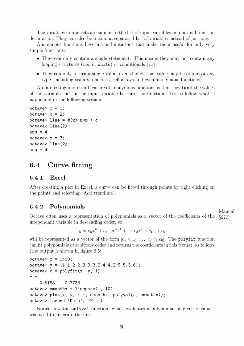
The variables in brackets are similar to the list of input variables in a normal functiondeclaration. They can also be a comma separated list of variables instead of just one.

Anonymous functions have major limitations that make them useful for only verysimple functions:

• They can only contain a single statement. This means they may not contain anylooping structures (for or while) or conditionals (if).

• They can only return a single value, even though that value may be of almost anytype (including scalars, matrices, cell arrays and even anonymous functions).

An interesting and useful feature of anonymous functions is that they bind the valuesof the variables not in the input variable list into the function. Try to follow what ishappening in the following session:

octave> m = 1;

octave> c = 2;

octave> line = @(x) m*x + c;

octave> line(2)

ans = 4

octave> m = 3;

octave> line(2)

ans = 4

6.4 Curve fitting

6.4.1 Excel

After creating a plot in Excel, a curve can be fitted through points by right clicking onthe points and selecting “Add trendline”.

6.4.2 PolynomialsManual§27.5Octave often uses a representation of polynomials as a vector of the coefficients of the

intependant variable in descending order, so

y = cnxn + cn−1x

n−1 + · · · c2x2 + c1x + c0

will be represented as a vector of the form [cn cn−1 . . . c2 c1 c0]. The polyfit functioncan fit polynomials of arbitrary order and returns the coefficients in this format, as follows(the output is shown in figure 6.5:

octave> x = 1:10;

octave> y = [1.1 2 2.3 3 3.2 4 4.2 5 5.3 6];

octave> c = polyfit(x, y, 1)

c =

0.5158 0.7733

octave> smoothx = linspace(1, 10);

octave> plot(x, y, ’.’, smoothx, polyval(c, smoothx));

octave> legend(’Data’, ’Fit’)

Notice how the polyval function, which evaluates a polynomial at given x values,was used to generate the line.

60

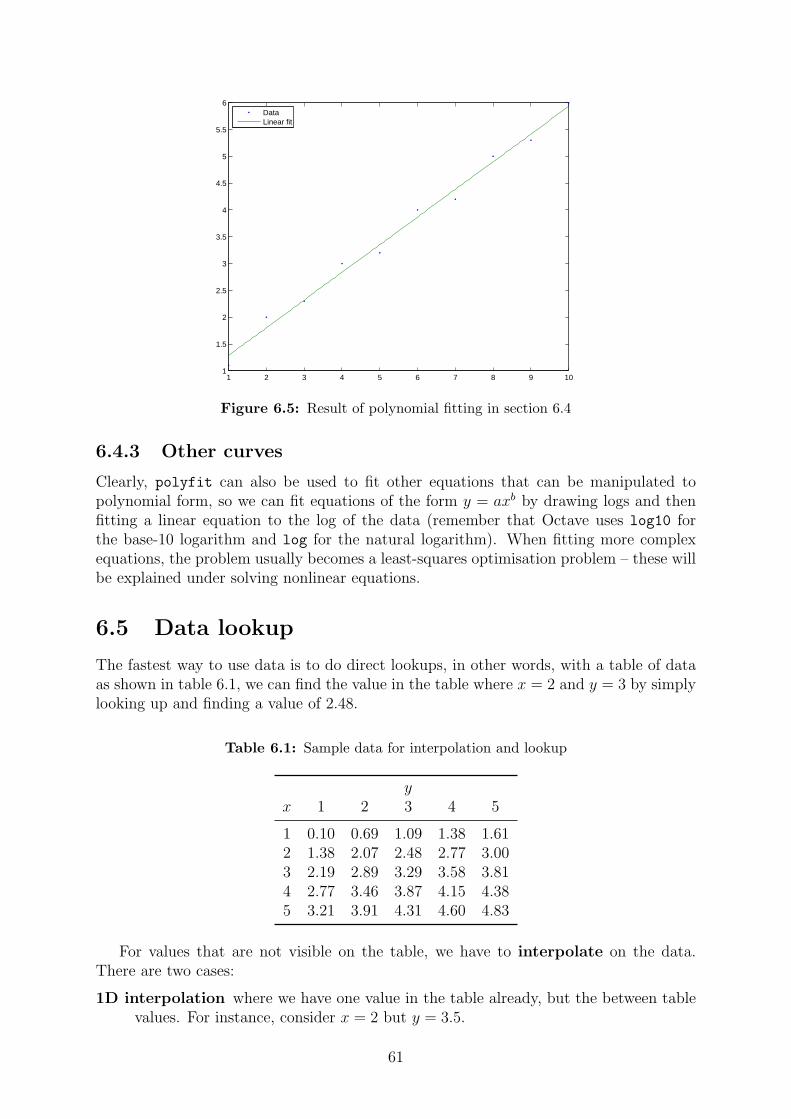
1 2 3 4 5 6 7 8 9 101

1.5

2

2.5

3

3.5

4

4.5

5

5.5

6

DataLinear fit

Figure 6.5: Result of polynomial fitting in section 6.4

6.4.3 Other curves

Clearly, polyfit can also be used to fit other equations that can be manipulated topolynomial form, so we can fit equations of the form y = axb by drawing logs and thenfitting a linear equation to the log of the data (remember that Octave uses log10 forthe base-10 logarithm and log for the natural logarithm). When fitting more complexequations, the problem usually becomes a least-squares optimisation problem – these willbe explained under solving nonlinear equations.

6.5 Data lookup

The fastest way to use data is to do direct lookups, in other words, with a table of dataas shown in table 6.1, we can find the value in the table where x = 2 and y = 3 by simplylooking up and finding a value of 2.48.

Table 6.1: Sample data for interpolation and lookup

yx 1 2 3 4 5

1 0.10 0.69 1.09 1.38 1.612 1.38 2.07 2.48 2.77 3.003 2.19 2.89 3.29 3.58 3.814 2.77 3.46 3.87 4.15 4.385 3.21 3.91 4.31 4.60 4.83

For values that are not visible on the table, we have to interpolate on the data.There are two cases:

1D interpolation where we have one value in the table already, but the between tablevalues. For instance, consider x = 2 but y = 3.5.

61

2D interpolation where we have both values between table values, for instance x = 3.2,y = 2.3.

Interpolation can be done using many different functions to approximate the inter-mediate behaviour. The best approximation, of course, is a model of the system inquestion. However, it is common practise to interpolate linearly or cubically (by fittinga line between the closest two points or a cubic between points with constraints on thederivatives). In the 1D case, this is easy to imagine – just draw a line between twopoints. In the 2D case, it is not as easy, but one can do a two-step interpolation, firstinterpolating for two data points for the rows above and below the desired value, theninterpolating between these points for the column.

6.5.1 Excel

In Excel, lookup in tables is handled by the VLOOKUP and HLOOKUP functions, that dovertical and horizontal lookups. They require a value to look up, a block of data and anoffset (how many rows or columns to move to the right or down to find the data value).The Excel help has good examples on how these functions work.

Interpolation is not as easy – one way is to do lookup for the closest values and thenuse the TREND function to give function values at new x values. If the data can be fit bya curve, one can fit the curve and use the equation to fill in missing values.

6.5.2 OctaveManual§28Octave supplies a rich set of functions to do interpolation via the interp1 (1D interpo-

lation) and interp2 (2D interpolation) functions. interp1 accepts an x and y vectorof known values and returns the values interpolated according to an optional method(doc interp1 for more information). interp2 accepts x and y vectors and a matrixcorresponding to the values in these vectors in addition to the x and y values at whichthe interpolation is to occur. It also has several options that are detailed in the help(doc interp2 for more information).

6.6 Integration

6.6.1 Quadrature

Quadrature is the determination of the area under a curve using numeric methods ratherthan analytic integration. The quad function accepts a function handle and two limits,and calculates the area under the curve defined by the function between the limits. Forinstance, take the function

y =sin(x)

x + 1(6.1)

which has no analytic integral.The function is plotted in figure 6.6To find the area ∫ π

0

sin(x)

x + 1dx

we can call quad with an anonymous function representing the equation we are integrat-ing:

62

0 1 2 3 4 5 6−0.2

−0.1

0

0.1

0.2

0.3

0.4

0.5

x

sin(

x)/(

x+1)

A1 ≈ 0.8438

A2 ≈ −0.3553

Figure 6.6: Quadrature example

octave> myfun = @(x) sin(x)./(x + 1);

octave> quad(myfun, 0, pi)

ans = 0.84381

Verify that you can obtain the second area as shown on the graph. What is the totalarea under the graph?

6.6.2 PolynomialsManual§27.4Using the curve fitting functions from section 6.4, we can fit a fourth order polynomial

to the function in equation 6.1

octave> myfun = @(x) sin(x)./(x + 1);

octave> smoothx = linspace(0, 2*pi);

octave> cfit = polyfit(smoothx, myfun(smoothx), 4);

Plot the function and the fitted polynomial to verify the fit is good over the interval wehave chosen.

Instead of using quad to calculate an approximate area, we can use the polyint

function to find the integral of the fitted polynomial, then find the area by evaluating theintegral polynomial at the values we desire.

octave> integralc = polyint(cfit);

octave> polyval(integralc, pi)

ans =

0.8432

63

6.7 Solving equations

6.7.1 Polynomials

Matlab offers many polynomial functions, and most of them start with poly followedby the function they represent. roots is the exception to this rule. It determines theroots of a polynomial described as discussed in section 6.4.2. Let’s find the roots of thepolynomial we fitted to equation 6.1 in section 6.6.2.

octave> roots(cfit)

ans =

7.2304

6.3163

3.1395

-0.0195

It is clear that the correct roots at x = 0, x = π and x = 2π are found, along with aspurious root outside the fitted x range.

roots is guaranteed to find all the roots of the polynomial, and will return complexroots as well.

6.7.2 Sets of linear equations

Sets of linear equations can be solved using matrix algebra. Make sure that you under-stand that the equations

a11x1 + a12x1 + a13x1 = b1

a21x1 + a22x1 + a23x1 = b2

a31x1 + a32x1 + a33x1 = b3

Can be simplified to the following: a11 a12 a13

a21 a22 a23

a31 a32 a33

x1

x2

x3

=

b1

b2

b3

Or, Ax = b. To solve for x, we simply multiply from the left by A−1, yielding A−1Ax =x = A−1b.

Octave

In Octave, muliplying from the left by the inverse of a matrix is done by the \ operator.It is helpful to think of this as ‘left division’ (as opposed to the ‘normal’ / right divisionoperator).

So, as an exaple, we may have the following statics problem where a beam is balancedon a hinge:

?

F1

?

F2

6

Fr

l1 l2

64

From a force and momentum balance, we can see that

F1 + F2 = Fr

l1F1 − l2F2 = 0

If l1 = 4 m, l2 = 6 m and Fr = 100 N, what are the values of F1 and F2?

octave> A = [1 1; 4 -6];

octave> b = [100; 0];

octave> F = A\b

F =

60

40

Excel

Excel also supplies matrix operations. The MMULT and MINVERSE functions calculate thematrix multiplication and matrix inverse of a region in Excel. The most important aspectof using array formulae in Excel is the use of Ctrl-Shift-Enter to enter the formula. Tryreworking the Octave example above in Excel.

6.7.3 Nonlinear equations

The fsolve function can be used to find the roots or zeros of a nonlinear function and isinvoked with a function to operate on and an approximate starting point near the zero inquestion. To use fsolve you have to define a function of one argument to find the zeroof. Often, the function we are dealing with has many arguments (one may for instanceneed physical constants, flowrates and other details). In such a case, it is often helpful tomake use of an anonymous function to operate as a wrapper for the real target function.

To continue with our example in equation 6.1, we can find the roots of this equationas follows:

octave> myfun = @(x) sin(x)./(x + 1);

octave> fsolve(myfun, 3)

ans = 3.1416

octave> fsolve(myfun, 7)

ans = 6.2832

Notice how fsolve only returns a root near the starting point value. This is becauseit is not generally known to the function how many roots it is looking for. Contrast thisto the roots function.

6.7.4 Sets of nonlinear equations

To find the solution to sets of nonlinear equations, it is common to rewrite them so thatthe right hand side is equal to zero.

So, if we had to find x and y such that

sin(x) + cos(y) = 0.3

x = 2− log(y)

65

We would first rewrite this to

sin(x1) + cos(x2)− 0.3 = 0

x1 + log(x2)− 2 = 0

Then, we would define a function to return a column vector containing the left handsides of the equations:

octave> system = @(x) [sin(x(1)) + cos(x(2)) - 0.3; x(1) + log10(x(2)) - 2];

octave> solutionx = fsolve(system, [2 2 ])

solutionx =

1.6301

2.3437

We can verify that this is indeed a solution by plotting the equations y = arccos(0.3−sin(x)) and y = 102−x and the solution obtained together

x = linspace(1, 3);

plot(x, acos(0.3-sin(x)), x, 10.^(2-x))

hold(’on’);

plot(solutionx(1), solutionx(2), ’ro’);

hold(’off’)

6.7.5 Excel Solver

Excel supplies an interface on optimisation called the solver, found under Tools|Solver(if the tool is not available, select Add-ins and select the check box next to solver). Thisinterface allows one to do optimisation of any cell in the spreadsheet by changing inputcells. Even though the solver interface is simple, it is very powerful, allowing one to addconstraints to the variables being solved for or on other cells.

An important aspect of using the solver is that it also requires an initial estimate ofthe values of the inputs before the optimisation can start.

6.8 Assignments

1. Write a function called colebrook which will solve for f ′ in the following nonlinearequation (the Colebrook estimator for the friction factor).

1√f ′ = −2 log

(e/D

3.7+

2.51

Re√

f ′

)The function must accept values for e, D, Re in that order and return the solution.

octave> colebrook(0.001, 100, 10000)

ans = 0.0309

66

2. It is known that haul truck speeds vary as a function of Total Resistance (RT )according to the function

V = Vmin + (Vmax − Vmin)(1 + e

RT−a

b

)−1

where Vmin and Vmax are the minimum and maximum speeds. Write a functioncalled truckfit that will accept two vectors – TR and V, and will return the fittingparameters a and b that fit the data by minimising the sum of the squares of theerror. Use the sqp function.

Test your function on this data (a ≈ −9.5, b ≈ 2.5):

TR 0 1 2 3 4 5 6 7 8 9 10 11 12V 52 52 52 51 50 47 45 41 37 32 27 22 18

3. Use Excel to plot and fit the data in the previous example. Use solver to find thevalues of the parameters. Save your spreadsheet as truckfit.xls

67

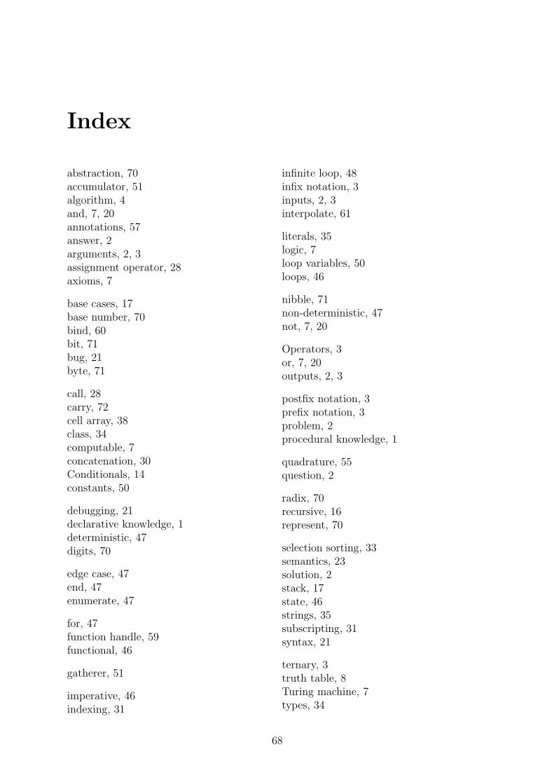
Index

abstraction, 70accumulator, 51algorithm, 4and, 7, 20annotations, 57answer, 2arguments, 2, 3assignment operator, 28axioms, 7

base cases, 17base number, 70bind, 60bit, 71bug, 21byte, 71

call, 28carry, 72cell array, 38class, 34computable, 7concatenation, 30Conditionals, 14constants, 50

debugging, 21declarative knowledge, 1deterministic, 47digits, 70

edge case, 47end, 47enumerate, 47

for, 47function handle, 59functional, 46

gatherer, 51

imperative, 46indexing, 31

infinite loop, 48infix notation, 3inputs, 2, 3interpolate, 61

literals, 35logic, 7loop variables, 50loops, 46

nibble, 71non-deterministic, 47not, 7, 20

Operators, 3or, 7, 20outputs, 2, 3

postfix notation, 3prefix notation, 3problem, 2procedural knowledge, 1

quadrature, 55question, 2

radix, 70recursive, 16represent, 70

selection sorting, 33semantics, 23solution, 2stack, 17state, 46strings, 35subscripting, 31syntax, 21

ternary, 3truth table, 8Turing machine, 7types, 34

68

Unary, 3undecidable, 7

value, 70values, 2variable scope, 28variables, 28

word, 71workspace, 28wrapper, 65

xor, 8

69

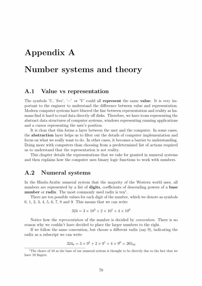
Appendix A

Number systems and theory

A.1 Value vs representation

The symbols ’5’, ’five’, ’:·:’ or ’V’ could all represent the same value. It is very im-portant to the engineer to understand the difference between value and representation.Modern computer systems have blurred the line between representation and reality as hu-mans find it hard to read data directly off disks. Therefore, we have icons representing theabstract data structures of computer systems, windows representing running applicationsand a cursor representing the user’s position.

It is clear that this forms a layer between the user and the computer. In some cases,the abstraction layer helps us to filter out the details of computer implementation andfocus on what we really want to do. In other cases, it becomes a barrier to understanding.Doing more with computers than choosing from a predetermined list of actions requiredus to understand that the representation is not reality.

This chapter details the representations that we take for granted in numeral systemsand then explains how the computer uses binary logic functions to work with numbers.

A.2 Numeral systems

In the Hindu-Arabic numeral system that the majority of the Western world uses, allnumbers are represented by a list of digits, coefficients of descending powers of a basenumber or radix. The most commonly used radix is ten1.

There are ten possible values for each digit of the number, which we denote as symbols0, 1, 2, 3, 4, 5, 6, 7, 8 and 9. This means that we can write

324 = 3× 102 + 2× 101 + 4× 100

Notice how the representation of the number is decided by convention. There is noreason why we couldn’t have decided to place the larger numbers to the right.

If we follow the same convention, but choose a different radix (say 9), indicating theradix as a subscript we can write

3249 = 3× 92 + 2× 91 + 4× 90 = 26510

1The choice of 10 as the base of our numeral system is thought to be directly due to the fact that wehave 10 fingers.

70

Negative powers are also allowed, allowing us to find representations of fractionalvalues by placing digits to the right of a fractional indicator (in South Africa we use ‘,’)so that

5

4= 1× 100 + 2× 10−1 + 5× 10−2 = 1, 25

When writing the representation of a value, we usually neglect any leading or trailingzeros, or zeros at the start of the representation of a number or to the right of the fractionalindicator, as they do not affect the value. It is, however, important to remember thatthere are theoretically an infinite number of zeros to the left of any integer representationand the right of any fractional representation, ie

1, 25 = · · · 0× 102 + 0× 101 + 1× 100 + 2× 10−1 + 5× 10−2︸ ︷︷ ︸1,25

+0× 10−3 · · ·

.In the computer world, hexadecimal notation is often used. This is a base 16 system,

and therefore has 16 unique single digits. The digits representing the values from 10 to15 are usually chosen as A-F, so that F416 = 15× 161 + 4× 160 = 244

A.2.1 Radix conversion

Any value can be represented in many different numeral systems, with many differentbases. We will not concern ourselves too much with different numeral systems, but wewill find it useful to convert between different bases.

When writing the value of a number using a different base number, we must find outhow to use only one digit for each power of the base number to describe the value we arelooking for. This means that we must fill up the number from left to right, so that wealways use the largest numbers available first.

To convert 26 to a binary (base 2) representation, we notice that the digits in binarywill correspond to 1, 2, 4, 8, 16, 32 and so on from right to left. The largest of thesenumbers that is less than 26 is 16. To convert the remainder, the same procedure isfollowed, so that 8 is the largest power of two less than 10, leaving 2 which is clearly apower of two. Our result is therefore

26 = 16 + 10

= 16 + 8 + 2

= 24 + 23 + 21

= 1 × 24 + 1 × 23 + 0 × 22 + 1 × 21 + 0 × 20

So we may write 2610 = 110102. This procedure is valid for any radix, and extends tofractional representation as well, so that 1, 2510 = 1, 012.

A.2.2 Computer terminology

Computer scientists refer to each binary digit as a bit. Names for groups of bits includea nibble for 4 bits, a byte for 8 bits and a word for a machine-natural number of bits2.Common word lengths are 16, 32 and 64 bits.

2Note that word length is machine specific, so different computers may have different definitions ofword

71

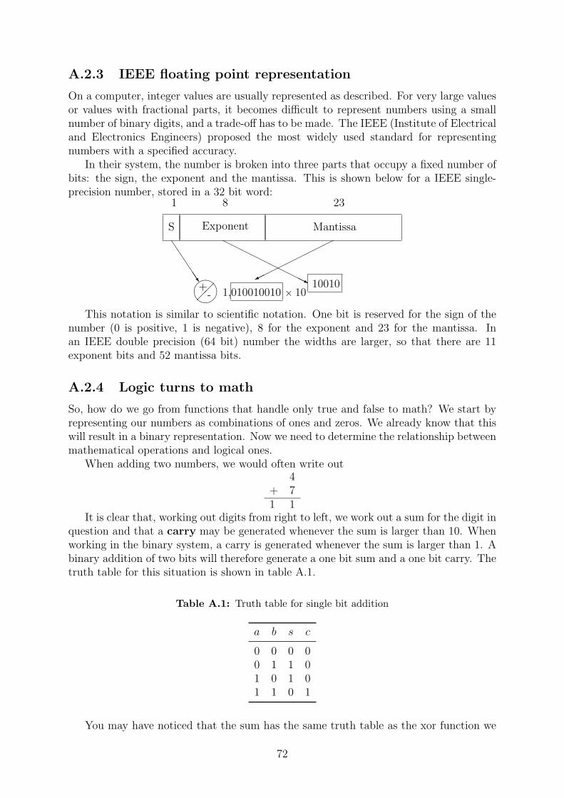
A.2.3 IEEE floating point representation

On a computer, integer values are usually represented as described. For very large valuesor values with fractional parts, it becomes difficult to represent numbers using a smallnumber of binary digits, and a trade-off has to be made. The IEEE (Institute of Electricaland Electronics Engineers) proposed the most widely used standard for representingnumbers with a specified accuracy.

In their system, the number is broken into three parts that occupy a fixed number ofbits: the sign, the exponent and the mantissa. This is shown below for a IEEE single-precision number, stored in a 32 bit word:

S Exponent Mantissa

����

JJ

JJJ

��

��

��

��

����

..........................

HH

HH

HH

HH

HHj

1 8 23

1,+

- 010010010 1010010

This notation is similar to scientific notation. One bit is reserved for the sign of thenumber (0 is positive, 1 is negative), 8 for the exponent and 23 for the mantissa. Inan IEEE double precision (64 bit) number the widths are larger, so that there are 11exponent bits and 52 mantissa bits.

A.2.4 Logic turns to math

So, how do we go from functions that handle only true and false to math? We start byrepresenting our numbers as combinations of ones and zeros. We already know that thiswill result in a binary representation. Now we need to determine the relationship betweenmathematical operations and logical ones.

When adding two numbers, we would often write out4

+ 71 1

It is clear that, working out digits from right to left, we work out a sum for the digit inquestion and that a carry may be generated whenever the sum is larger than 10. Whenworking in the binary system, a carry is generated whenever the sum is larger than 1. Abinary addition of two bits will therefore generate a one bit sum and a one bit carry. Thetruth table for this situation is shown in table A.1.

Table A.1: Truth table for single bit addition

a b s c

0 0 0 00 1 1 01 0 1 01 1 0 1

You may have noticed that the sum has the same truth table as the xor function we

72

just defined, and that the carry is generated only when both inputs are true, just like theand function. It should be clear that s = a xor b, while c = a · b.

In a similar manner, we can define functions that return the digits for any numberof bits added together by connecting several logic functions together. This is the basisof computer arithmetic. Of course, the circuits that do multiplication or division areconsiderably more complex, but they can all be expressed as combinations of and, or andnot.

A.3 Assignments

1. Write a function radixvalue that will take a vector of digits d and a radix r and re-turn the value of the representation. For instance, 2203 = 24, so radixvalue([2 2 0], 3)

will return 24.

>> radixvalue([1 0 2 0 3], 4)

ans =

291

>> radixvalue([1 2 0 3], 6)

ans =

291

For extra credit, use only one line for this program.

2. Write a function valueradix that will take a number n and a radix r and return avector containing the digits of the representation of n in the radix r.

>> valueradix(24, 3)

ans =

2 2 0

>> valueradix(291, 4)

ans =

1 0 2 0 3

>> valueradix(291, 6)

ans =

1 2 0 3

Hint: One way of doing radix conversion is by repeatedly dividing the value by theradix and writing down the remainder. This gives the digits from least significantto most significant. So converting 24 to radix three we find 24/3 is 8, remainder0 . 8/3 is 2 remainder 2 . 2/3 is 0 remainder 2 . We stop when we attempt to dothis with 0. Our conversion shows 24 = 2203. The floor function may be useful.

73