Computational Topology for Geometric and

Molecular Approximations

Edward L. F. Moore, Ph.D.University of Connecticut, 2005

The goal of this research will be to provide sufficient conditions and tractable al-gorithms that guarantee the topological embedding of geometric approximationscommonly used by modern geometric design systems. Particular focus is on theuse of ambient isotopy as the measure of topological equivalence, which is stricterthan the more traditional use of homeomorphism. Such topological guaranteeswill be made within a user-specified tolerance for applications specific to futureComputer-Aided Geometric Design (CAGD) and Computer-Aided Molecular De-sign (CAMD) systems. The results of this work contribute to the emerging fieldof computational topology, while providing more accurate and efficient modelingmethods to the geometric and molecular design communities.

Computational Topology for Geometric and

Molecular Approximations

Edward L. F. MooreB.S.M.E., University of Florida, 1993

M.S.M.E., University of Central Florida, 1998

A DissertationSubmitted in Partial Fullfilment of the

Requirements for the Degree ofDoctor of Philosophy

at theUniversity of Connecticut

2005

Copyright by

Edward L. F. Moore

2005

APPROVAL PAGE

Doctor of Philosophy Dissertation

Computational Topology for Geometric and

Molecular Approximations

Presented byEdward L. F. Moore,

Major Advisor

Thomas J. PetersAssociate Advisor

Alexander C. RussellAssociate Advisor

John A. Roulier

University of Connecticut2005

ii

ACKNOWLEDGEMENTS

iii

TABLE OF CONTENTS

1. Introduction . . . . . . . . . . . . . . . . . . . . . . . . . . . . . . . . 11.1 Contributions . . . . . . . . . . . . . . . . . . . . . . . . . . . . . . . 21.2 Thesis overview . . . . . . . . . . . . . . . . . . . . . . . . . . . . . . 3

2. Background . . . . . . . . . . . . . . . . . . . . . . . . . . . . . . . . 42.1 Topological definitions . . . . . . . . . . . . . . . . . . . . . . . . . . 52.1.1 Combinatorial topology . . . . . . . . . . . . . . . . . . . . . . . . 52.1.2 Point-Set topology . . . . . . . . . . . . . . . . . . . . . . . . . . . 72.1.3 Embedded topology . . . . . . . . . . . . . . . . . . . . . . . . . . 102.2 Knot theory . . . . . . . . . . . . . . . . . . . . . . . . . . . . . . . . 132.3 Homeomorphic subdivision . . . . . . . . . . . . . . . . . . . . . . . . 152.4 Piecewise Linear(PL) approximations . . . . . . . . . . . . . . . . . . 172.5 Weierstrass approximation theorem . . . . . . . . . . . . . . . . . . . 20

3. The Class of Unknots with Knotted Control Polygons . . . . . 21

4. Isotopic Curve Subdivision . . . . . . . . . . . . . . . . . . . . . . 274.1 Subdivision of planar and open curves . . . . . . . . . . . . . . . . . 274.2 Subdivision in R

3 for degree less than 5 . . . . . . . . . . . . . . . . . 284.3 On the number of subdivisions . . . . . . . . . . . . . . . . . . . . . . 324.4 Experimental examples . . . . . . . . . . . . . . . . . . . . . . . . . . 35

5. Isotopic Surface Approximation . . . . . . . . . . . . . . . . . . . 385.1 Isotopy of a surface by control points . . . . . . . . . . . . . . . . . . 405.2 Manifolds with Boundary . . . . . . . . . . . . . . . . . . . . . . . . 42

6. Algorithms . . . . . . . . . . . . . . . . . . . . . . . . . . . . . . . . 446.1 Isotopic curve subdivision algorithm . . . . . . . . . . . . . . . . . . 446.2 Star algorithm . . . . . . . . . . . . . . . . . . . . . . . . . . . . . . 446.3 Applications . . . . . . . . . . . . . . . . . . . . . . . . . . . . . . . . 46

7. Conclusion . . . . . . . . . . . . . . . . . . . . . . . . . . . . . . . . . 47

Bibliography 48

iv

LIST OF FIGURES

2.1 Same graphs, different objects . . . . . . . . . . . . . . . . . . . . . . 72.2 (a) Block. (b) Block with slot. (c) Block with hole. . . . . . . . . . . 82.3 Union between a solid 3-manifold cube and a 2-manifold planar surface:

(a) before the union, and (b) resultant mixed-dimensional object . 102.4 (a) The Unknot (b) The Non-Planar Trefoil knot . . . . . . . . . . . 112.5 Non-Equivalent Knots . . . . . . . . . . . . . . . . . . . . . . . . . . 122.6 The first three knots (a) The unknot 01 (b) The trefoil knot 31 (c) The

figure-8 knot 41 . . . . . . . . . . . . . . . . . . . . . . . . . . . . 132.7 (a) A messy unknot (b) The unknot . . . . . . . . . . . . . . . . . . 142.8 Cubic B-spline curve with knot vector (a) {0 0 0 0 1 1 1 1}, (b) {0 0 0

0 .5 .5 .5 1 1 1 1}, (c) {0 0 0 0 .25 .25 .25 .5 .5 .5 .75 .75 .75 1 1 1 1} 162.9 Cubic B-spline curve with knot vector (a) {0 0 0 0 1 1 1 1}. (b) {0 0

0 0 .5 .5 .5 1 1 1 1}. . . . . . . . . . . . . . . . . . . . . . . . . . . 172.10 (a) The unknot. (b) The figure-8 knot. (c) Good approximation. . . . 182.11 A curve with its pipe surface and PL approximant. . . . . . . . . . . 19

3.1 Non-self-intersecting degree 10 Bezier curve with self-intersecting con-trol polygon. . . . . . . . . . . . . . . . . . . . . . . . . . . . . . . 22

3.2 (a) Non-self-intersecting degree 10 Bezier curve with knotted controlpolygon (b) Same curve rotated about the y-axis . . . . . . . . . . 25

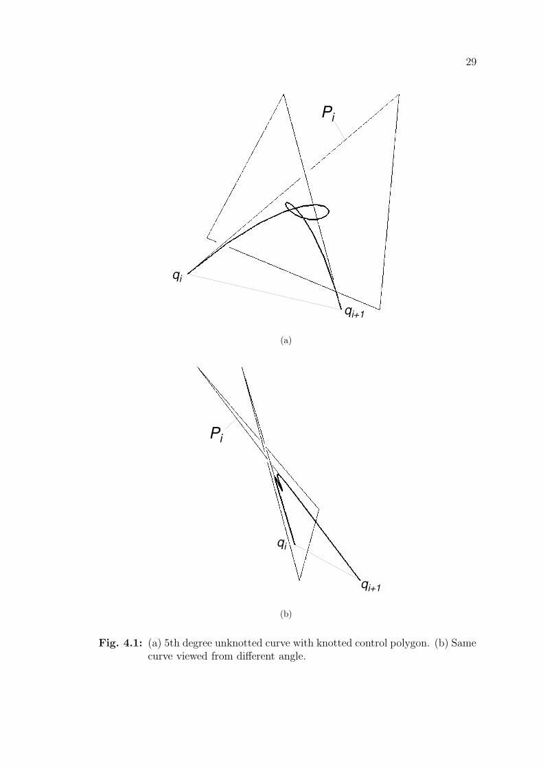
4.1 (a) 5th degree unknotted curve with knotted control polygon. (b) Samecurve viewed from different angle. . . . . . . . . . . . . . . . . . . 29

4.2 Normal plane does not give good sets of compact support. . . . . . . 304.3 (a) 4th degree curve segment. (b) Two 4th degree curve segments

’pasted’ together . . . . . . . . . . . . . . . . . . . . . . . . . . . 334.4 The control points are ’pushed’ along the linear path denoted by the

dashed arrows. . . . . . . . . . . . . . . . . . . . . . . . . . . . . 344.5 A cubic bezier curve (a) with no subdivisions (b) after 1st subdivision

(c) after 2nd subdivision, and (d) control polygon of 3rd subdivisionfits inside pipe surface. . . . . . . . . . . . . . . . . . . . . . . . . 36

6.1 (a) Star(v) (b) Star(v*) . . . . . . . . . . . . . . . . . . . . . . . . . 45

v

LIST OF TABLES

vi

Chapter 1

Introduction

Topology is the branch of mathematics that studies the properties of geometricobjects which are preserved under continuous deformation [1]. Whereas geometryis concerned with rigid form, size and location of objects, topology is concernedwith deformation, connectivity, and associativity of objects.

The field of computational geometry as its own discipline has been pervasivein CAGD, computer graphics, and robotics for more than twenty years [2]. Theterm ‘computational topology’ first appeared in 1983 to emphasize the role of thetopological adjacency relationships within CAGD [3]. More recently, researchersare attempting to formalize computational topology into its own discipline [4] inan effort to improve reliability in geometric computing, varying in scales from theatomic to the astronomical.

The nascent field of computational topology holds great promise for re-solving several long-standing industrial design modeling challenges. Geometricmodeling has become commonplace in industry as manifested by the critical useof Computer Aided Geometric Design (CAGD) systems within the automotive,aerospace, shipbuilding and consumer product industries. Commercial CAGDpackages depend upon complementary geometric and topological algorithms. Theemergence of geometric modeling for molecular simulation and pharmaceuticaldesign presents new challenges for supportive topological software within Com-puter Aided Molecular Design (CAMD) systems. For both CAGD and CAMDsystems, splines provide relatively mature geometric technology for modeling com-plex shapes. However, there remain robustness issues regarding the ’topology’ ofthese models, particularly for supporting simulations that rely upon approxima-tions of these models. The simultaneous consideration of CAGD and CAMDis important to provide unifying abstractions to benefit both domains. In engi-neering applications it is a common requirement that topological equivalence bepreserved during geometric modifications, but in molecular simulations attentionis focused upon where topological changes have occurred as indications of impor-tant chemical changes. The methods presented in this thesis are supportive ofboth these disciplinary approaches.

An important challenge in computational topology is the development ofrigorous, robust and tractable methods for guaranteeing that computational ap-

1

2

proximations of smooth curves and surfaces preserve critical topological charac-teristics. Such treatments of topology are lacking in the contemporary literature,and become the focus of contribution in this thesis to computational topology.

1.1 Contributions

This thesis furthers the field of computational topology by contributing formal-izations of algorithmic issues in topology and topological considerations for com-puter applications. Both emphases are combined to create algorithms to ensurethat geometric approximations are sufficiently accurate to maintain topologicalequivalence for robust modeling within CAGD and CAMD. As a result of this re-search, the following three contibutions are made to the scientific and engineeringcommunity.

1. The ’topology’ of a CAGD model is frequently expressed as a critical prop-erty for reliable engineering simulation. Although topology is a well formal-ized subject in mathematics, communication about the topology of CAGDmodels is ambiguous in the computational and engineering literature. Inthis thesis, precise terminology is defined for communicating about CAGDand CAMD models with the goal of providing a foundation for future de-velopment of software systems capable of more robust simulations. Thus, ifone speaks of preserving the topology of a geometric model or changing thetopology of a model by some operation on the model, it is important to spec-ify which topological characteristics are of interest, where the focus of thisresearch is on preserving ambient isotopy. Such definitions will contribute tobetter communication about topological modeling in the geometric designliterature.

2. Using ambient isotopy as the criteria for equivalence is a stronger guaran-tee for approximations than the traditional use of homeomorphism. Theisotopic subdivision algorithm proposed in Theorem 4.2.1 for subdivisionapproximations will be useful for geometric design systems that performapproximations for display and analysis. Both engineering and molecularapplications will require accurate topology while intersecting surfaces dy-namically during simulations. A challenging test area could be on DNAmolecules, where structure and function are inextricably related, since DNAmostly exists in a supercoiled form – meaning it is twisted and tangled (andknotted) in order to be in a state of minimum energy [5–7]. Ambient isotopicapproximations are shown for both Bezier curves and spline surfaces.

3. The local and global topology preservation under the star algorithm for 1-complexes is expected to be useful in simulating properties of higher dimen-sional complexes having in excess of ten thousand vertices. In particular,

3

earlier work [8,9] relied upon the expensive computation of all distances be-tween disjoint vertices, edges and faces. It was specifically noted [8] thatthese computations could be done prior to any single perturbation. How-ever, when many perturbations are being executed, the overhead associatedwith repeating that full computation for each iteration may be prohibitive.The more localized methods proposed here afford significant performanceadvantages when relevant. Hence, further refinement and development ofthe star algorithm will contribute to more efficient and robust algorithmsfor geometric and molecular simulations.

1.2 Thesis overview

The remainder of this dissertation is organized as follows. Chapter 2 contains thebackground in topology that is needed to understand the sequel. Much of thismaterial is available in standard texts, to which the interested reader is referred formore details. Chapter 3 is the central motivation and compelling example for theinvestigations that follow concerning the role of knottedness in control polygonsand their associated spline curves and surfaces. This relies upon a projectionlemma, which is proved in this chapter, but which is expected to be a well-known‘folk theorem’. The value of this lemma, though, is that it can be used in ageneral technique to create unknotted Bezier curves whose control polygons areknotted, as shown in this chapter. Hence, consideration of this phenomenonis seen as not being restricted to pathological cases, but has wide applicability.Chapter 4 contains one of the principal results, indicating that repeated subdvisionof a Bezier curve of degree less than 5 will eventually create a control polygonhaving the same isotopy class as the curve. The advantages of this method overother techniques for curve approximation are presented, with a particular focusupon examples that show the algorithmic gains made by this approach. Thereasons for the degree restriction are discussed, with some indications for futuregeneralizations. Chapter 5 then has partial extensions of these curve results tosurfaces, with discussions of the present limitations of those extensions. Chapter 6presents the pseudocode to transform the previous theory into effective algorithms,as well as discussion of current and emerging application opportunities. The finalchapter contains conclusions.

Chapter 2

Background

Surprisingly, all contemporary CAGD systems lack the reliability and robustnessrequired for automation of sophisticated engineering analysis tasks such as com-putational fluid dynamics (CFD), finite element analysis (FEA) and optimizationof design processes. These engineering applications rely heavily on the accuracy ofthe model provided by the original CAGD system. An intermediate step betweenCAGD and analysis is the generation of a piecewise linear (PL) mesh which in-troduces added errors from the mesh approximation of a free-form surface. Whilemeshing is typical in CAGD, it is expected to become more prominent in CAMDas more sophisticated surface models of molecules evolve. During model approx-imations for engineering analysis, topological anomalies that now arise includeextraneous self-intersections, unwarranted gaps, and incorrect connectivity – allof which can cause problems in a subsequent analysis. According to Farouki [10],a core problem with modern CAGD systems is in the underlying mathematicsused for representing models, and the source of many of these problems arise fromthe algorithmic issues inherent in computing approximations. The mismatch be-tween approximate geometry and faithful topology has historically caused relia-bility problems not only in CFD and FEA, but also for scientific visualizationand engineering applications. As CAMD matures, with more sophisticated geo-metric models, the accompanying visualizations and simulations are expected toexperience similar approximation problems. Hence, it is useful to consider thetopological characteristics of the approximation problem from the viewpoints ofCAGD and CAMD simultaneously.

Modern engineering simulation increasingly relies upon geometric modelsto analyze a broad range of objects, from manufactured parts to bio-molecularsystems. Today’s CAGD and CAMD systems lack the reliability and robustnessrequired for automation of analysis tasks such as CFD, FEA, and design optimiza-tion [10]. Such analyses typically require computations on application-specific ap-proximations of these models. Furthermore, many operations in commercial solidmodeling packages perform approximations “under the hood” without providingany awareness to the end user. Most notable is the intersection between two

4

5

surfaces, where, for example, each surface may be a B-spline given by [11],

S(u, v) =

n∑

i=0

m∑

j=0

Ni,p(u)Nj,q(v)Pi,j (2.1)

where the Ni,p(u) and Ni,q(v) are the pth-degree and qth-degree B-spline basisfunctions, the {Pi,j} are the control points, and (u, v) ∈ [0, 1]2. Such surface in-tersection routines typically approximate the intersection curve with a low degreepiecewise polynomial curve, since the theoretically exact result may be too highof a degree to be computationally efficient [12]. Clearly, this raises open ques-tions. How good is a particular approximation? What criteria should be usedto determine a ’valid’ approximation for a particular analysis? Current theoryand methods for evaluating topological equivalence of approximations is eithermisleading or simply not considered. Hence, a key milestone towards achievinghigher reliability, lower human intervention, and faster results for engineering sim-ulations is the ability to algorithmically guarantee topologically correct geometricapproximations.

This chapter presents background material and key definitions that are usedthroughout this thesis. Section 2.1 presents the most important definitions intopology for this work. Sections 2.3 and 2.4 discuss important related work leadingto the main results of this thesis in Chapter 4. Finally, Section 2.2 provides somebackground on the theory of mathematical knots.

2.1 Topological definitions

In order to make progress in engineering and molecular simulations, with theirdependency upon topology, the use of precise terminology is important. In par-ticular, this is in sharp contrast to informal usage, which frequently just speaksof the ’topology of a model’. For the purposes of this thesis to aid in the develop-ment of future CAGD and CAMD systems, the following three areas of topologyare proposed as fundamental: Combinatorial Topology, Point-Set Topology, andEmbedded Topology.

2.1.1 Combinatorial topology

The underlying idea here is that each geometric object is defined, as is typical ina solid modeling boundary representation (see below), by a collection of points,curves and surfaces, which respectively are called nodes, edges and faces. For thistheoretical view of the representation, each node is assumed to lie on a curve andto limit the extent of the curve. Typically, each curve will have two limiting nodes,an initial node and a final node. A well-known example is the use of the notation[0,1] to represent the interval from 0 to 1 that is inclusive of these two end-points.

6

These end-points are also known as the boundary of the curve. Similarly, eachsurface will be limited by a collection of curves that forms its boundary. Thistype of topology is also often referred to as symbolic topology because of the datarepresentation practice of taking each geometric entity and assigning some uniquesymbol to it. This prevents redundant storage of data. For instance, considertrying to represent the triangle with nodes:

(0, 0, 0), (1, 0, 0), (0, 1, 0)

The three edges could, in turn, be listed as

[(0, 0, 0), (1, 0, 0)]

[(1, 0, 0), (0, 1, 0)]

[(0, 1, 0), (0, 0, 0)]

with the triangular boundary then indicated by the cyclic list

{[(0, 0, 0), (1, 0, 0)], [(1, 0, 0), (0, 1, 0)], [(0, 1, 0), (0, 0, 0)]}

However, it is more convenient to make the following symbolic assignments

(0, 0, 0) → A

(1, 0, 0) → B

(0, 1, 0) → C

Then the edges can be listed as

[A, B] → E1

[B, C] → E2

[C, A] → E3

and the triangle then becomes the cyclic list

{E1, E2, E3}

This level of indirection is particularly important to preserve data integritywhen the nodes have co-ordinates represented by floating point values, which istypical.

It is easy to see that this combinatorial topology can be represented in agraph, where the nodes take on symbols, as indicated above. In this context,preservation of topology could mean that these symbolic graphs are identical fortwo objects or that they are isomorphic. If one wishes the graphs to be identical,

7

then the represented objects can still appear very differently to the user. Forinstance, a triangle and a disc could have exactly the same symbolic topologygraph, but the geometric entities referenced for the triangle would be line segmentswhereas those for the disc would be arcs, as shown in Figure 2.1. If one wishes thebroader equivalence of isomorphic graphs, then this raises the well-known graphisomorphism problem, for which it remains unknown as to whether answers arecomputationally tractable. However, it is well-known that changing the graph canstill preserve topological equivalence of the object from a point-set perspective, asdiscussed in Section 3.2.

A

B C

A

B C

A

B CGraph

TriangleDisc

Fig. 2.1: Same graphs, different objects

The relationship between the location of one entity relative to another isdefined here as adjacency. Adjacency information is typically at the core of anyCAGD system, and their symbolic representation is critical for Boolean operationssuch as union, intersection, and subtraction between two solids. Many data struc-tures have been proposed and studied over the past twenty-five years for sufficientstorage of adjacency information within the context of combinatorial topology.However, the design of these data structures will not be discussed any further,and the reader is referred to [13,14] for more details.

2.1.2 Point-Set topology

Point-set topology is a mature mathematical subject completely independent ofany reference to solid modeling. However, it is somewhat surprising that thedominant use of topology in solid modeling has been in the sense described inSection 2.1.1 without much regard to the point-set implications. Equivalencerelations are central to topology. A central definition in point-set topology is ahomeomorphism.

8

Definition 2.1.1: Any two subsets X and Y of R3 are homeomorphic if there

exists a function f : X → Y such that f is continuous, 1 − 1, has a continuousinverse and maps onto all of Y . Such a function is known as a homeomorphism.

In the context of CAGD, a homeomorphism is intuitively expressed in thefollowing example. Consider the three blocks shown in Figure 2.2. Figure 2.2(a)is merely a parallelpiped. Figure 2.2(b) is a block with a slot, and the blockin Figure 2.2(c) contains a hole. Imagine that each object is made of an ex-tremely pliable or rubber-like material. Note that there exists a homeomorphismbetween the block and the block with the slot since each object can be continu-ously deformed into the other. However, there does not exist a homeomorphismbetween the block and the block with the hole because the object would have tobe ’punctured’ in order to produce the hole. Hence, there can be no continuoustransformation between the block and the block with a hole. It is also worthwhileto note that each of the three blocks would have very different adjacency graphsin order to represent their combinatorial topology. Hence, the adjacency graph,alone, is inconclusive towards determining the classical topological equivalencegiven by homeomorphisms. Consider then the block and a block with a slot in it,as shown in Figure 2.2. They would have very different symbolic graphs to repre-sent the combinatorial topology of each. However, there exists a homeomorphismbetween these objects.

(a) (b) (c)

Fig. 2.2: (a) Block. (b) Block with slot. (c) Block with hole.

Within the context of point-set topology, it is worthwhile to distinguishfour topological characteristics important to the practice of CAGD: connectivity,multiple-points 1, number of components, and dimensionality. Connectivity is theformal topological term for what most design engineers would informally refer toas a ’hole’ or ’gap’ in the model. Indeed, there are several refinements of the ideaof connectivity, and it is noted that a hole will mean that some local region isnot simply connected. As this is a deep concept, it is only mentioned here that

1 Multiple-points are more commonly called self-intersections in the literature

9

a hole on a surface will prevent a loop on that surface from being continuouslycontracted to a point within that surface. These holes can either be intentionallypart of a model or an unwanted artifact from an approximation. If the latter is thecase, then the unwanted hole can dramatically affect an engineering simulation.

Multiple-points occur when a geometric object intersects itself. Typically,multiple points are an unwanted artifact of some operation intended to approxi-mate the original model, and similar to what was discussed regarding connectivitycharacteristics, undesirable artifacts here also interfere with reliable engineeringsimulation. It is clear that multiple points fit nicely within the context of point-settopology: an approximation with an unwanted self-intersection does not have aone-to-one correspondence with the original model. Hence, the approximation isnot homeomorphic to the original model.

Solid models can be composed of multple shells, where each shell is definedas having its adjancency graph of nodes, edges and faces being disjoint fromany other adjacency graph in the model. Hence, two distinct shells correspondnicely to the point-set topology concept of two sets being contained in open setswhose closures are disjoint [1]. There exists a minimal number for this family ofcomplementary closed sets such that this number is a topological invariant of thesolid, meaning that if these numbers are different for two solids, then these twosolids cannot be homeomorphic. This minimal number is equal to the number ofcomponents within point-set topology [1].

Finally, the dimensionality of a model is defined as follows. Most CAGDsystems, particularly those referred to as solid modelers, are designed to onlyrepresent n-manifolds, where n is either one, two, or three in each component.Formally, an n-manifold is a space such that each point of the space is containedin an open set which is homeomorphic to an open subset of R

n or an open subsetof a closed half-space of R

n. For example, any open or closed space curve, whichis allowed to self-intersect only at its end points, is a 1-manifold. Similarly, anon-self-intersecting surface is a typical example of a 2-manifold and a solid is a3-manifold. Most data structures used in commercial CAGD systems to repre-sent the connective and adjacency relationships restrict Boolean operands to bemanifolds having the same value of n (This also implies that the resultant is ann-manifold.)

Consider what can happen if these input constraints were relaxed. For in-stance, if one takes the set-theoretic union (not the Boolean operation of ‘join’,which is sometimes informally discussed in CAGD communities as ‘union’) of a3-manifold cube with the 2-manifold surface shown with the ‘dashed’ lines in Fig-ure 2.3(a), the set-theoretic result would be the object in Figure 2.3(b) consistingof the new 3-manifold cube with a ’dangling’ 2-manifold [15,16]. Most commercialCAGD systems in use today use data structures that will not allow for such a re-sult. Indeed, although what is depicted in Figure 2.3(b) is a perfectly valid set, itis not an admissible result of a Boolean operation [17]. However, there are systems

10

in use that employ more complex data structures [14] allowing the representationof mixed dimensional objects, and in this case, the operation in Figure 2.3(a) isdefined. Consistent with the literature, these types of representations are callednon-manifold [14], and the types of representations that do not allow multipledimensions in a single component are called manifold. This is important becauseit represents another method to distinguish when two objects are homeomorphic.Obviously, any manifold object is not homeomorphic to any non-manifold, andmanifold objects of different dimensions are not homeomorphic.

(a) (b)

Fig. 2.3: Union between a solid 3-manifold cube and a 2-manifold planar surface:(a) before the union, and (b) resultant mixed-dimensional object

2.1.3 Embedded topology

While the relations of combinatorial topology and the equivalence relations definedby homeomorphisms are quite powerful and useful, they fail to distinguish betweentwo types of objects that most engineering professionals would choose to placein different equivalence classes. For instance, if set A is a circle and set B is aknotted curve (See Figure 2.4), then there exists a homeomorphism between them,yet it is often useful to distinguish between these two curves. Indeed, this can beaccomplished with additional topological techniques. Intuitively, two closed curveswill be in different equivalence classes if one knot can only be converted into theother by untying and retying it to conform to the other. This relates to how thetwo objects are situated within R

3, which is formally known as an embedding,and any function which preserves this embedding is known as an ambient isotopy.

Definition 2.1.2: Let X and Y be two subspaces of Rn. Then there is an am-

bient isotopy, H between X and Y if there exists a continuous function H :R

n × [0, 1] → Rn with the following conditions:

1. H(·, 0) is the identity,

2. H(X, 1) = Y , and

3. ∀t ∈ [0, 1], H(·, t) is a homeomorphism from Rn onto R

n.

11

The sets X and Y are then said to be ambient isotopic.

Although any two simple closed planar curves are ambient isotopic, twosimple homeomorphic space curves, need not be ambient isotopic, because theycan describe different knots. For instance, the simplest possible knot is planarand is a circle, and this is known as the unknot or the trivial knot. Any nontrivialknot must necessarily be non-planar, and the simplest nontrivial knot is the trefoilknot. Both these knots are depicted in Figure 2.4, where one should note the threeovercrossings in space for the trefoil knot, leading to its name. Indeed, the numberof crossings is a critical discriminant for different knot equivalence classes and theinterested reader is referred to the standard text [6] for more background. Anytwo knots will be in the same equivalence class determined by homeomorphisms,but can still be in very different equivalence classes as determined by ambientisotopies. These different knot equivalence classes become particularly relevantwhen considering the piecewise linear (PL) approximations of free-form geometrythat are often used for engineering analyses.

(a) (b)

Fig. 2.4: (a) The Unknot (b) The Non-Planar Trefoil knot

For defining ambient isotopies, it is often sufficient to restrict the movementof points to a compact subset of R

n, allowing the function to be the identityoutside this compact set. This property also permits easier decision about when agiven function is an ambient isotopy, as attention can be focused to local, ratherthan global, behavior of the function. This property is well-known and is defined,below, as compact support.

Definition 2.1.3: A function f , from the space X to X has compact supportif there is a compact set K ⊆ X such that for any x ∈ X − K, f(x) = x. Then,K is called a set of compact support for f .

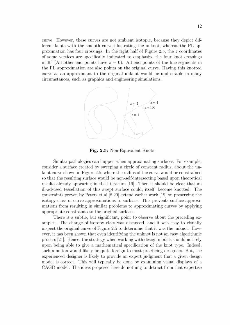
It has been shown [18] that in creating a PL approximation of a smoothunknot that it is possible to change the knot equivalence class, referred to here asknottedness. That example is repeated here. Figure 2.5 shows two simple home-omorphic space curves, where the PL curve is an approximation of the smooth

12

curve. However, these curves are not ambient isotopic, because they depict dif-ferent knots with the smooth curve illustrating the unknot, whereas the PL ap-proximation has four crossings. In the right half of Figure 2.5, the z coordinatesof some vertices are specifically indicated to emphasize the four knot crossingsin R

3 (All other end points have z = 0). All end points of the line segments inthe PL approximation are also points on the original curve. Having this knottedcurve as an approximant to the original unknot would be undesirable in manycircumstances, such as graphics and engineering simulations.

z = -2z = 100

z = -1

z = -1

z = 1

Fig. 2.5: Non-Equivalent Knots

Similar pathologies can happen when approximating surfaces. For example,consider a surface created by sweeping a circle of constant radius, about the un-knot curve shown in Figure 2.5, where the radius of the curve would be constrainedso that the resulting surface would be non-self-intersecting based upon theoreticalresults already appearing in the literature [19]. Then it should be clear that anill-advised tessellation of this swept surface could, itself, become knotted. Theconstraints proven by Peters et al [8,20] extend earlier work [19] on preserving theisotopy class of curve approximations to surfaces. This prevents surface approxi-mations from resulting in similar problems to approximating curves by applyingappropriate constraints to the original surface.

There is a subtle, but significant, point to observe about the preceding ex-amples. The change of isotopy class was discussed, and it was easy to visuallyinspect the original curve of Figure 2.5 to determine that it was the unknot. How-ever, it has been shown that even identifying the unknot is not an easy algorithmicprocess [21]. Hence, the strategy when working with design models should not relyupon being able to give a mathematical specification of the knot type. Indeed,such a notion would likely be quite foreign to most practicing designers. But, theexperienced designer is likely to provide an expert judgment that a given designmodel is correct. This will typically be done by examining visual displays of aCAGD model. The ideas proposed here do nothing to detract from that expertise

13

and judgment, but, instead, the methods proposed rely entirely upon such soundjudgments. Namely, the formalisms discussed here can lead to software tools toensure that if the topology of a model is judged to be correct, then subsequentgeometric approximations will not alter that topology, if the approximations areappropriately constrained.

Note that such circumstances may even be relevant to the pathologies dis-cussed by Farouki [10]. For instance, the smooth and approximating curves shownin Figure 2.5 are both non-self-intersecting. However, again, a slight variant of thisexample could be generated where the original curve was non-self-intersecting andthe other contained a self-intersection. This type of difference can be determinedin that the non-self-intersecting object and the self-intersecting object would bediscriminated purely via point-set topology, where they would be in different topo-logical equivalence classes determined by homeomorphisms. For such differences,there is no need for the more powerful techniques based on ambient isotopy, butthe proposed topological constraints will also ensure against changing the topo-logical equivalence class determined by homeomorphisms. Recall that one of thepathologies mentioned in [10] is that self-intersections can appear in models wherenone are expected. If such self-intersections were generated in a model approxi-mation process, then the constraints discussed here will prevent that.

2.2 Knot theory

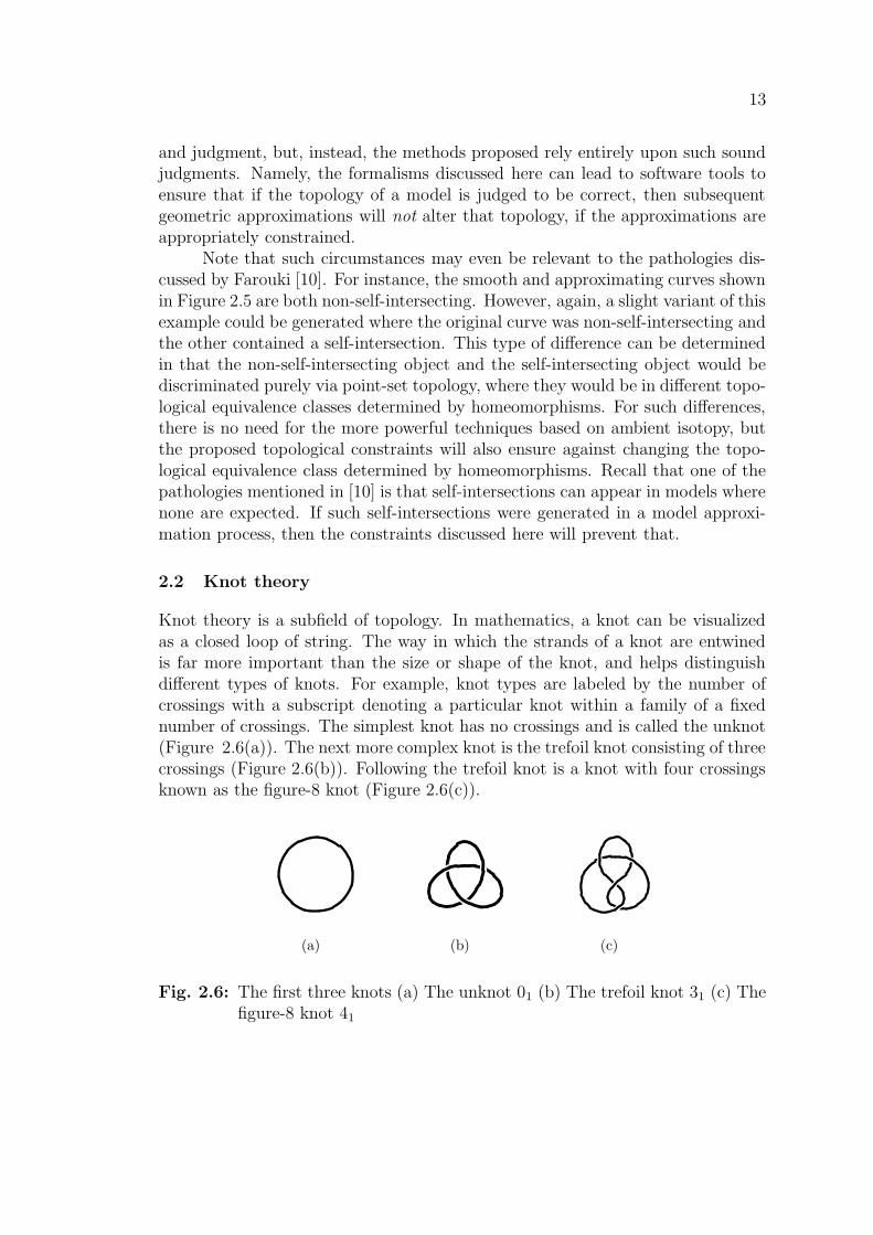
Knot theory is a subfield of topology. In mathematics, a knot can be visualizedas a closed loop of string. The way in which the strands of a knot are entwinedis far more important than the size or shape of the knot, and helps distinguishdifferent types of knots. For example, knot types are labeled by the number ofcrossings with a subscript denoting a particular knot within a family of a fixednumber of crossings. The simplest knot has no crossings and is called the unknot(Figure 2.6(a)). The next more complex knot is the trefoil knot consisting of threecrossings (Figure 2.6(b)). Following the trefoil knot is a knot with four crossingsknown as the figure-8 knot (Figure 2.6(c)).

(a) (b) (c)

Fig. 2.6: The first three knots (a) The unknot 01 (b) The trefoil knot 31 (c) Thefigure-8 knot 41

14

Knot theory also studies links. Links are simply two or more knots that mayor may not be entwined in such a way that they can not be separated withoutbreaking one of the knots.

The fundamental questions in knot theory are how to distinguish differenttypes of knots, how to determine knot equivalence, and how to recognize whethera “tangled mess” is actually knotted. Two knots can appear to be drasticallydifferent geometrically, yet topologically they are the same. Note that the knotin Figure 2.7(a) is actually the unknot. It can be continuously deformed into theunknot shown in Figure 2.7(b) without breaking a single strand. Good introduc-tory texts on knot theory are offered by Adams [5], Gilbert and Porter [22], andLikorish [23].

(a) (b)

Fig. 2.7: (a) A messy unknot (b) The unknot

Mathematicians have investigated knot theory for nearly a hundred yearswith some of the most exciting results occurring over the last two decades. Themost active area of research is finding polynomial invariants to distinguish knots.Historically, the first polynomial invariant was published by J. Alexander [24], andthe Alexander polynomial along with simple generalizations remained the onlyknot invariant in existence for 60 years until the discovery of a new polynomialinvariant by Vaughan Jones [25] in 1984. The significance of Jones’ discoverywas that unlike the Alexander polynomial, the Jones polynomial could distinguishmost of the time whether a knot is equivalent to its mirror image. Many invariantsnow exist, but no single invariant can distinguish all knots.

The work presented here on correct topology for geometric approximationsis expected to have impact upon a broad range of technical disciplines such asengineering, biology, chemistry and physics. For example, Molecular Biologistsnow realize the use of knot theory for the modeling and simulation of molecularstructure found in DNA molecules [26–28] and proteins, which depend upon thetopologically correct geometric approximations for visualizations and animationof these molecular models. Similarly, such approximated geometric models willalso support visualization for chemists who are now researching knot theory as a

15

basis for the study of topological stereochemistry to model and synthesize complexmolecules [29].

2.3 Homeomorphic subdivision

Repeatedly subdividing a curve by uniformly inserting knots with multiplicityequal to the curve degree and then capturing its control polygon is a commontechnique for rapidly approximating a curve for display or analysis, as was firstcaptured by the Oslo algorithm [30]. The typical convergence of a control polygonvia subdivision is depicted in Figure 2.8. Figure 2.8(a) represents a simple cubicBezier curve B with control polygon P. The curve is then subdivided by insertingknots with multiplicity equal to three, as shown in Figure 2.8(b) and Figure 2.8(c).Note how rapidly the control polygon converges to the curve in terms of distance.

However, since self-intersecting control polygons can define non-self-intersectingcurves, one result [31] resolved that any non-self-intersecting curve will eventuallyhave a non-self-intersecting control polygon under repeated subdivision. This isdepicted in Figure 2.9, where the self-intersecting control polygon for the non-self-intersecting cubic B-spline in Figure 2.9(a) becomes non-self-intersecting bysubdividing the knot vector in Figure 2.9(b). Furthermore, the control polygoncan never again become self-intersecting under any successive subdivisions [31].The result depends upon the regularity of the parameterization. A regular param-eterization t ∈ [a, b] is one such that the 1st derivative of the curve does not vanishfor all values of t [32]. If the curve parameterization is not regular, then there arecases where a self-intersecting control polygon with a non-self-intersecting curvewill never become non-self-intersecting by repeated subdivision [31].

The stopping criteria for these recursive subdvision graphics algorithms areusually based upon the subdivision merely being within some numerical distancebound of the orginal curve. For instance, the initial control polygon here rep-resents the 0 − th subdivision, and, if this 0 − th subdivision satisfied merely adistance bound from the original curve for graphics display, then this would be aninappropriate rendering of the curve. Since subdivision is widely used in graphicsdisplay, additional care must be taken to ensure that not only is any approxima-tion within some distance of the original curve, but also that desired topologicalproperties should be preserved. The material in Chapter 4 provides theorems andexamples with explicit topological criteria for ambient isotopic subdivision.

This thesis studies whether the topological embedding of a spline curveis preserved by approximation of the control polygon through uniform subdivi-sion. The topological form of equivalence considered here not only considers self-intersections, but also considers the embedding of a curve in three-dimensionalspace. This relies upon equivalence by ambient isotopy, which is stronger thanthe more traditional equivalence relation given by homeomorphism. The mainresult presented in Chapter 4 proves the following theorem. Given a C2 spline

16

(a) (b)

(c)

Fig. 2.8: Cubic B-spline curve with knot vector (a) {0 0 0 0 1 1 1 1}, (b) {0 0 00 .5 .5 .5 1 1 1 1}, (c) {0 0 0 0 .25 .25 .25 .5 .5 .5 .75 .75 .75 1 1 1 1}

17

(a) (b)

Fig. 2.9: Cubic B-spline curve with knot vector (a) {0 0 0 0 1 1 1 1}. (b) {0 00 0 .5 .5 .5 1 1 1 1}.

curve with a clamped and uniform knot vector, the piecewise linear curve formedfrom the control points eventually becomes ambient isotopic to the curve by re-peated subdivision. As a direct result of this theorem, an algorithm to computeambient isotopic curve approximations is outlined in Chapter 6. The next sectiondiscusses piecewise linear approximations of spline curves, which provides morebackground for the main result presented in Chapter 4.

2.4 Piecewise Linear(PL) approximations

Summarizing previous work [18], the space curve in Figure 2.10(a) is equivalentto the unknot. An undesirable PL approximation, shown in Figure 2.10(b), isthe figure-8-knot. This crude approximation would not be acceptable for manyanalysis and visualization applications. However, the more refined approximationshown in Figure 2.10(c) is ambient isotopic to the original curve. While this ismerely an illustrative example, it suggests that similar changes in the embeddingcould occur during approximation by subdivision. The main theorem presented inSection 4.2 gives sufficient conditions to obtain an ambient isotopic approximationby repeated subdivision.

It is easy to see from the example in Figure 2.10 that if one displayed a pro-jection of this initial approximation as a graphics approximation of the curve, thenthe displayed graphics would have self-intersections, whereas the original curvedoes not. Indeed, the use of projections is fundamental in analyzing knots [5],as will be further indicated in the sequel, particularly in Chapter 3. Hence, this

18

(a) (b) (c)

Fig. 2.10: (a) The unknot. (b) The figure-8 knot. (c) Good approximation.

lends some caution to the typical graphics practice of using an approximation ofa curve for its display. Summarizing previous work [19], it has been shown howto generate an ambient isotopic PL approximation of a curve in R

3. The resultrelies upon understanding pipe surfaces, so their definition follows2.

Definition 2.4.1: The pipe surface of radius r of a parametrized curve c(t),where t ∈ [0, 1] is given by

p(t, θ) = c(t) + r[cos(θ)n(t) + sin(θ)b(t)],

where θ ∈ [0, 2π] and n(t) and b(t) are, respectively, the normal and bi-normalvectors at the point c(t), as given by the Frenet-Serret trihedron.

Then the previous ambient isotopic PL approximation proof [19] follows fourmain steps, under the assumption that c is C2:

1. Determine a radius r such that p(t, θ) is non-self-intersecting.

2. Define Nr(c) to be the open neighborhood of c with boundary given byp(t, θ) if c is a closed curve. If c is an open curve then the two closed discsof radius r normal to c at its endpoints must be added to this boundary.

3. Select points {q0, q1, . . . , qn} on c such that each line segment [qi, qi+1] lieswithin Nr(c) (where [qn, qn+1] = [qn, q0].) Furthermore, denoting each sec-tion of c between qi and qi+1 as ci, each ci is ambient isotopic to [qi, qi+1]via the nearest point mapping.

4. The open polyline with vertices {q0, q1, . . . , qn} is ambient isotopic to c, if cis open, otherwise the closed polyline on {q0, q1, . . . , qn} is ambient isotopicto c.

2 Pipe surfaces have been studied since the 19th century [33], but the presentation here followsa contemporary source [34].

19

For use later in this thesis, the r-pipe isotopy property is now defined basedon these four criteria.

Definition 2.4.2: If the set Q = {q0, q1, . . . , qn} on a curve has the four proper-ties listed above, then Q will be said to have the r-pipe isotopy property.

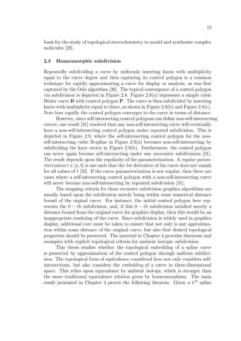
Considering Figure 2.11, let ci be the segment of c between qi and qi+1, letDi be the closed disc of radius r normal to c at qi and let pi be the section ofthe pipe surface between Di and Di+1. Then, the previously published proof [19]constructs local ambient isotopies from [qi, qi+1] to ci for each i, such that eachlocal isotopy has a set of compact support bounded by

Di ∪ pi ∪ Di+1.

Each Di remains fixed under the local isotopies, so the proof is then completedby reliance upon the following “folk lemma” (even though this reliance was notspecifically articulated). This lemma provides sufficient conditions so that two dif-ferent isotopies defined over intersecting sets of compact support can be “pasted”together to yield a single ambient isotopy over the union of the sets of compactsupport.

Di Di+1

qi i+1q

pi

N (c)rc

Fig. 2.11: A curve with its pipe surface and PL approximant.

This result from the literature relies upon the idea that local isotopies can bejoined together to form an overall isotopy. This article [19] does not supply thosemathematical details, as they are particularly easy to follow within their proof.However, a more generalized argument is needed, later, in Chapter 4, to supportthe main proof. Hence, that associated “Ambient Isotopic Pasting Lemma” ispresented and proved in Chapter 4.

20

2.5 Weierstrass approximation theorem

The Weierstrass Approximation Theorem is of fundamental importance and prac-ticality for computing applications that evaluate a broad variety of functions. Itproves how any continuous real-valued function on a compact interval can be uni-formly approximated by a sequence of polynomials. The results presented in Chap-ter 5 on isotopic surface approximations are similar in spirit and were partiallymotivated by this fundamental topological approximation theorem. Analogously,it will be shown how compact orientable C2 manifolds can be approximated bya sequence of piecewise linear(PL) manifolds. For the special case of spline sur-faces, the vertices of the PL approximants can be specifically chosen with theintent of capturing additional shape characteristics of the original manifold. TheWeierstrass Approximation Theorem is now given here, where the notation [a, b]represents a closed interval in R, whenever a < b.

Theorem 2.5.1: Every real-valued continuous function f on [a, b] can be approx-imated uniformly by polynomials.

Proof: Please consult a standard topology reference, such as [35].

Note that the original function f is merely required to be continuous. Noother specific characteristics are known, such as whether it might be exponential.But, it then claims that a uniform approximation can be generated that is also acontinuous function. In an analogous spirit, we only identify that we have a C2

compact orientable manifold. It may be with or without boundary and we do notknow any specific information about its isotopy equivalence class. However, we arestill able to deliver an approximating compact manifold that is ambient isotopic tothe original. Usually, the approximant created will no longer be C2, differing fromhow the Weierstrass Approximation Theorem preserves continuity. However, thisloss of surface smoothness is not often an issue in computing applications. Indeed,the interest often is primarily in generating a piecewise linear (PL) approximationfor use in graphics, simulations and engineering analysis software packages [30].Moreover, since two surfaces can be isotopic while having very different shapes3,the approximation of spline surfaces that is created in chapter 5 is based uponthe control points of those surfaces, since these control points offer additionalinformation about the underlying shape.

3 Consider the unit sphere and the PL boundary of the unit cube.

Chapter 3

The Class of Unknots with Knotted Control Polygons

The following example motivates the need for ambient isotopic subdivision.Consider the planar Bezier curve shown in Figure 3.1. The graphics appear

to show that this planar curve is non-self-intersecting. However, knowing thatgraphics can obscure some subtleties (particularly since each graphical image isonly an approximation to some pixel level accuracy), it is important to conducta more rigorous analysis to conclude that any curve is truly non-self-intersecting.The graphics can be suggestive and helpful, but rarely can they be considered tobe conclusive. That more detailed analysis is undertaken here and is presented,below.

Initial consideration of planar curves is fundamental to the methodologypresented here to generate arbitrarily many examples unknotted curves whosecontrol polygons are non-trivial knots. This methodology relies upon the followingtwo results. The first is likely a ‘folk theorem’ and the second is a standard result.

Lemma 3.0.1 (Unknot Projection Test): If K is a knot such that some pla-nar projection of K is non-self-intersecting, then K is the unknot.

Proof: Without loss of generality, assume that the projection is into the planein R

3 defined by z = 0 and that the projection is denoted by π. Since π(K) isnon-self-intersecting, there does not exist z1 6= z2 such that (x, y, z1) ∈ K and(x, y, z2) ∈ K. Hence, K cannot have any over-crossing or under-crossings in R

3,implying that K must be the unknot.

Lemma 3.0.2 (Projection of Bezier Curves): The parallel projection of a Beziercurve is achieved by applying the same projection to its control points.

Proof: See [11], specifically the discussion on p. 236.

Hence, these two results can be applied to some non-self-intersecting Bezierplanar curves to generate unkotted space curves that have knotted control poly-gons. The obvious idea is to consider the planar Bezier curve as a projectionof some space curve. As long as the planar curve can be shown to be non-self-intersecting, its pre-image under the projection cannot be knotted, due to

21

22

Fig. 3.1: Non-self-intersecting degree 10 Bezier curve with self-intersecting con-trol polygon.

23

Lemma 3.0.1. Without loss of generality, the ensuing exposition will be simplifiedby assuming that the plane of interest is the x-y plane, with an implied z valueof 0. Hence, if the co-ordinates of the control points of the planar curve are alsorepresented as (x, y, z) ordered triples, then it is clear that changes in only thez-values would not change the planar Bezier curve generated by a projection ontothe x-y plane by Lemma 3.0.2. However, it should also be clear that this raises thepossibility to change the z co-ordinates to create a knotted control polygon. Anexample follows with the same degree 10 Bezier curve shown in Figure 3.1. Thishigh degree was chosen merely for numerical and graphical convenience. However,it is interesting to note that this construction will only generate the described ex-amples when the degree of the Bezier curve is at least 5, as will be explained inmore detail in the next chapter, due to a known result on ‘stick knots’.

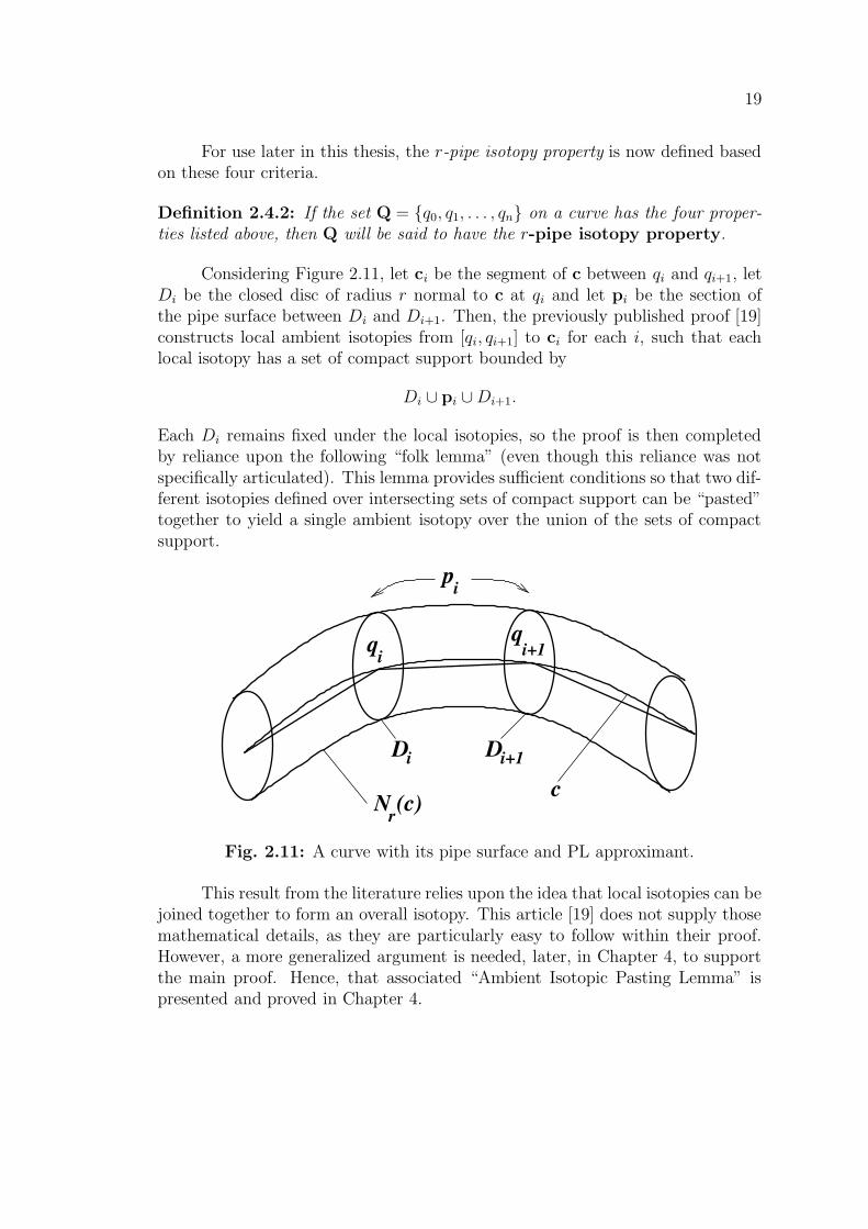
The example depicted Figure 3.1 above has the following planar controlpoints:

P0 = (2.25, 0)

P1 = (6, 0)

P2 = (6,−2.25)

P3 = (4,−2.25)

P4 = (4,−5.75)

P5 = (4.875,−1.9375)

P6 = (5.75,−5.5)

P7 = (0,−5.5)

P8 = (0, 0)

P9 = (1.375, 0)

P10 = (2.25, 0)

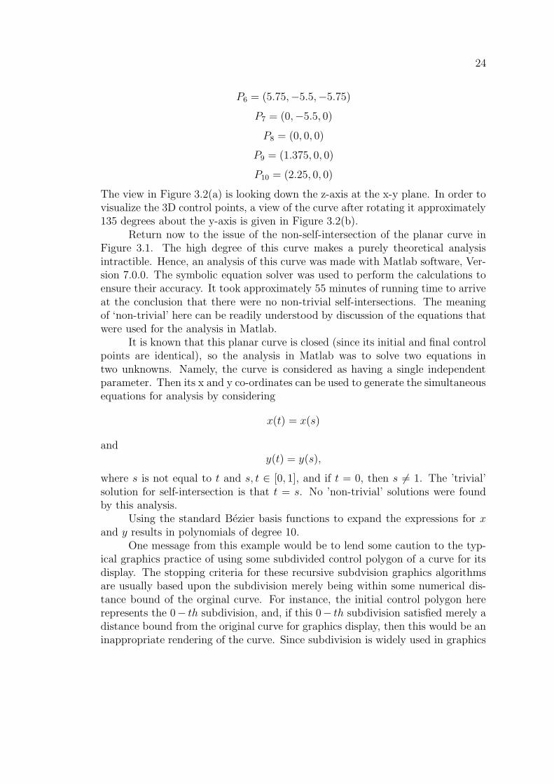
By applying a z co-ordinate to particular control points above, it is clear thata knotted control polygon can result. A specific example resulting in controlpolygon which is a figure-8 knot is shown in Figure 3.2(a). The control points forthis example are as follows:

P0 = (2.25, 0, 0)

P1 = (6, 0, 0)

P2 = (6,−2.25, 14.5)

P3 = (4,−2.25, 0)

P4 = (4,−5.75,−4.5)

P5 = (4.875,−1.9375, 7.5)

24

P6 = (5.75,−5.5,−5.75)

P7 = (0,−5.5, 0)

P8 = (0, 0, 0)

P9 = (1.375, 0, 0)

P10 = (2.25, 0, 0)

The view in Figure 3.2(a) is looking down the z-axis at the x-y plane. In order tovisualize the 3D control points, a view of the curve after rotating it approximately135 degrees about the y-axis is given in Figure 3.2(b).

Return now to the issue of the non-self-intersection of the planar curve inFigure 3.1. The high degree of this curve makes a purely theoretical analysisintractible. Hence, an analysis of this curve was made with Matlab software, Ver-sion 7.0.0. The symbolic equation solver was used to perform the calculations toensure their accuracy. It took approximately 55 minutes of running time to arriveat the conclusion that there were no non-trivial self-intersections. The meaningof ‘non-trivial’ here can be readily understood by discussion of the equations thatwere used for the analysis in Matlab.

It is known that this planar curve is closed (since its initial and final controlpoints are identical), so the analysis in Matlab was to solve two equations intwo unknowns. Namely, the curve is considered as having a single independentparameter. Then its x and y co-ordinates can be used to generate the simultaneousequations for analysis by considering

x(t) = x(s)

andy(t) = y(s),

where s is not equal to t and s, t ∈ [0, 1], and if t = 0, then s 6= 1. The ’trivial’solution for self-intersection is that t = s. No ’non-trivial’ solutions were foundby this analysis.

Using the standard Bezier basis functions to expand the expressions for xand y results in polynomials of degree 10.

One message from this example would be to lend some caution to the typ-ical graphics practice of using some subdivided control polygon of a curve for itsdisplay. The stopping criteria for these recursive subdvision graphics algorithmsare usually based upon the subdivision merely being within some numerical dis-tance bound of the orginal curve. For instance, the initial control polygon hererepresents the 0− th subdivision, and, if this 0− th subdivision satisfied merely adistance bound from the original curve for graphics display, then this would be aninappropriate rendering of the curve. Since subdivision is widely used in graphics

25

(a)

(b)

Fig. 3.2: (a) Non-self-intersecting degree 10 Bezier curve with knotted controlpolygon (b) Same curve rotated about the y-axis

26

display, additional care must be taken to ensure that not only is any approxima-tion within some distance of the original curve, but also that desired topologicalproperties should be preserved. The next chapter gives explicit topological criteriato be met and provides theorems and examples for doing so.

Chapter 4

Isotopic Curve Subdivision

The new results presented here are dependent upon three results from the litera-ture. First, a fundamental result is that repeated subdivision permits arbitrarilyclose approximation of a spline curve [30]. Second, a recent topological perspec-tive is that any spline curve having no self-intersections will eventually have anon-self-intersecting control polygon under repeated subdivision [31]. Third, theresult presented in [19] given in Section 2.4 constructed an ambient isotopic PLapproximation to a spline curve, but did not use subdivision.

The results presented here provide advantages over the approach taken inthe previously cited literature [19]. Namely, that earlier work will guarantee anambient isotopic approximation, if the user is able to judiciously choose interpolantpoints for a PL approximation such that each of the approximating linear segmentslies within the stipulated pipe surface. Hence, the user must pick a collection ofpoints and then test for geometric inclusion of each of the generated line segments.This could take many iterations, with no clear information about stopping criteria.The approach developed here provides two advantages

• the approximating line segments are generated by sub-division, so thereis no need for the user to guess at appropriate points, where subdivisionalgorithms are quite standard and stable, and

• additional results can be integrated to give formal a priori stopping criteriaas to the number of iterations required to have the control polygon fit withinthe stipulated pipe surface.

The second item, above, requires further explanation, which is provided laterin Section-4.3. This chapter begins by first presenting some easy results for thepurely planar case of curves in Section 4.1. These are included primarily for thesake of completeness, but the real emphasis here is upon space curves, as given inSection 4.2.

4.1 Subdivision of planar and open curves

For isotopic planar subdivision, the knottedness of the curve is not consideredsince the isotopy occurs in R

2. Similarly, for subdivision of an open curve in R3

27

28

with degree less than five, the knottedness of the curve is not considered sincean open curve does not describe a knot (note: the degree < 5 constraint will bedescribed in Section 4.2. Hence, only self-intersections need to be considered whenperforming subdivision approximation on either a planar curve (open or closed)or an open curve in R

3. Furthermore, the degree of the curve is not important forthe planar case, in contrast to subdividing curves in R

3, as will be shown in thenext two sections.

Theorem 4.1.1: Let B be a non-self-intersecting C2 Bezier curve with regularBezier parametrization, where B is open or closed in the plane or B is open inR

3 with degree < 5. Let P be the control polygon defined by the control points ofB. Then P is eventually ambient isotopic to B under repeated subdivision.

Proof: Subdivide the curve until P is non-self-intersecting [31]. Any two opennon-self-intersecting and non-planar curves are ambient isotopic. Also, any twoclosed, non-self-intersecting, non-planar curves are ambient isotopic.

Note that this may provide an option for the graphics community to gen-erally continue to use subdvision to preserve isotopy without too much concern.Namely, many curves are only displayed after planar projection. Hence, if a curveis projected as non-self-intersecting onto a plane, then eventually subdivision willyield a non-self-intersecting control polygon, which could then be used for display.

4.2 Subdivision in R3 for degree less than 5

This section discusses subdivision for curves with degree less than five. Extendingthe current theory to curves in R

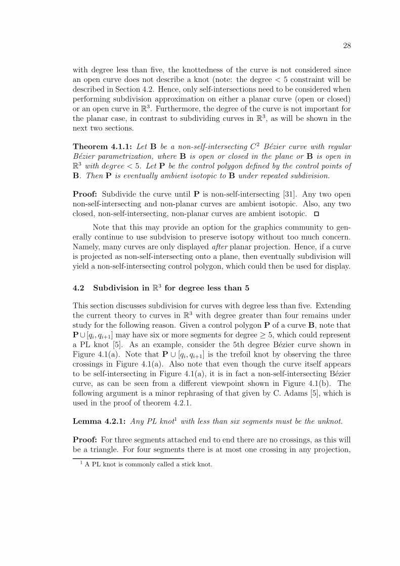
3 with degree greater than four remains understudy for the following reason. Given a control polygon P of a curve B, note thatP∪ [qi, qi+1] may have six or more segments for degree ≥ 5, which could representa PL knot [5]. As an example, consider the 5th degree Bezier curve shown inFigure 4.1(a). Note that P ∪ [qi, qi+1] is the trefoil knot by observing the threecrossings in Figure 4.1(a). Also note that even though the curve itself appearsto be self-intersecting in Figure 4.1(a), it is in fact a non-self-intersecting Beziercurve, as can be seen from a different viewpoint shown in Figure 4.1(b). Thefollowing argument is a minor rephrasing of that given by C. Adams [5], which isused in the proof of theorem 4.2.1.

Lemma 4.2.1: Any PL knot1 with less than six segments must be the unknot.

Proof: For three segments attached end to end there are no crossings, as this willbe a triangle. For four segments there is at most one crossing in any projection,

1 A PL knot is commonly called a stick knot.

29

(a)

(b)

Fig. 4.1: (a) 5th degree unknotted curve with knotted control polygon. (b) Samecurve viewed from different angle.

30

so such a knot is trivial. For five segments, a projection can be made of foursegments while looking down the fifth segment. Such a projection can have atmost one crossing, corresponding to the unknot. Since a trefoil knot can be madefrom six segments, six is the minimum number of segments required to make anon-trivial knot.

A remark was previously made in Chapter 2 about the technique used tocreate the ambient isotopy within the pipe surface [19]. Crucial to their resultwas the property that each Di contained only the single common endpoint ofthe consecutive segments [qi, qi+1] and [qi+1, qi+2]. The circumstances are notso simple when considering control polygons. For instance, consider Figure 4.2which is centered about the origin. The plane normal to the curve at (0, 0, 0)intersects five points of the control polygon, so no subset of this plane can playthe previous role of Di. The proof of the main curve approximation theorem below(theorem 4.2.1) relies upon an assumption that Pi ∪ [qi, qi+1] is the unknot.

Fig. 4.2: Normal plane does not give good sets of compact support.

Fortunately, a slightly more elaborate technical argument yields the moregeneralized result that is used within the ensuing proof.

Lemma 4.2.2 (Ambient Isotopic Pasting Lemma): For n ≥ 0, let F be anambient isotopy defined on R

n × [0, 1] onto Rn so that subsets A and B of R

n

are ambient isotopic under F . Similarly, let G be an ambient isotopy defined onR

n × [0, 1] onto Rn so that subsets C and D of R

n are ambient isotopic underG. Furthermore, suppose that F has compact support CS(F ) and G has compactsupport CS(G). If for each point x ∈ CS(F ) ∩ CS(G), it is true that F (x, t) =G(x, t) = x, for all t ∈ [0, 1], then there exists an ambient isotopy of compactsupport mapping A ∪ C onto B ∪ C.

Proof: The functionH : R

n × [0, 1] → Rn,

defined by

H(x, t) =

F (x, t), x ∈ CS(F ),G(x, t), x ∈ CS(G),x, otherwise;

31

for t ∈ [0, 1] is an ambient isotopy with compact support CS(F ) ∪ CS(G) suchthat A ∪ C is ambient isotopic to B ∪ D under H.

Now, it must be shown that (a) H(x, t) is continuous ∀t ∈ [0, 1], and (b)that H(x, t) is a homeomorphism ∀t ∈ [0, 1] in order for H(x, t) to be an ambientisotopy. For (a), H(x, t) is continuous as a direct application of the pasting lemmain [1]. For (b), Let t ∈ [0, 1], and consider H(x, t) for each x ∈ R

n. If x ∈ CS(F ),then H(x, t) is a homeomorphism by definition of H, since H(x, t) = F (x, t). Ifx ∈ CS(G), then H(x, t) is a homeomorphism, since H(x, t) = G(x, t). Similarly,if x /∈ CS(F ) ∪ CS(G), then H(x, t) is a homeomorphism, since H(x, t) = x.

There is a third technical consideration about how to show that a stickknot with 5 sticks yields the type of local ambient isotopy required to satisfyLemma 4.2.2. Fortunately, this can readily be done, as indicated in the followinglemma.

Lemma 4.2.3: Consider the unknot formed with 5 sticks. Then, 4 consecutivesticks can be made ambient isotopic to the 5th stick by an isotopy where the endpoints of the 5th stick remain fixed.

Proof: Label the vertices as v1, v2, v3, v4, v5. Assume, without loss of generality,that the fixed segment is [v1, v2], and that the indices are cyclic along the arclengthof the stick knot.

Then perturb v4 so that it is collinear with v3 and v5. This can be done bya single push [36], resulting with a quadrilateral, where the vertex v4 is no longerimportant. By perturbing, v3, all four remaining verticies are can be guaranteedto be co-planar. It is then easy to see that 2 planar pushes will produce the desiredisotopy with compact support that leaves v1 and v2 fixed.

With these technical preliminaries in place, it is now possible to state andprove the principle isotopic approximation result for Bezier curves.

Theorem 4.2.1: Let B be a non-self-intersecting C2 Bezier curve with regularBezier parametrization in R

3 where B also has degree less than five. Then thereexists a subdivision of B whose control polygon is ambient isotopic to B. Fur-thermore, there exists such a subdvision such that the control polygon of eachsubsequent subdivision is also ambient isotopic to B. (Note that B may be openor closed.)

Proof: For the curve B, choose a radius r for a pipe surface of B as defined inSection 2.4. Then, take sufficiently many subdivisions such that

• the control polygon is contained in Nr(B) (See Section 2.4), and

• the control polygon is non-self-intersecting [31] (See Section 2.3).

32

Then, let Q = {q0, q1, . . . , qn} be the subdivision points on B, noting thatQ meets the four criteria for a PL approximation to be isotopic to its curve givenin Section 2.4. Let Pi be the control polygon for each Bi. Two key points mustbe shown to complete the proof:

1. that there exists an ambient isotopy between each Pi and linear segmentconnecting [qi, qi+1] (See Figure 4.3(a)), and

2. that each segment of the curve can be ’pasted’ together to form a singleisotopy.

In order to show that there exists an ambient isotopy between each Pi andlinear segment connecting [qi, qi+1], the points qi and qi+1 must remain fixed. Then,each control point between qi and qi+1 is continuously moved to the line segment[qi, qi+1] along a linear path via a push [36] (See Figure 4.4), generlizing the 2Dpush defined by Bing [36] to 3D. These details are expressed here, for the sake ofcompleteness in Lemma 4.2.3, where it is noted that the perturbations expressedin Lemma 4.2.3 can be further constrained to lie within the neighborhood aboutthe curve constructed having the pipe surface as its boundary.

By applying lemmas 4.2.1 and 4.2.3, as indicated, there will be an ambientisotopy if the degree of the curve is less than five (i.e. less than six segments).

It is now clear that there exists an ambient isotopy between [qi, qi+1] and Pi,implying that each Pi is also ambient isotopic to Bi. Since these are all compactsets and each point qi remains fixed, the pasting lemma (See Section 2.4) can beapplied to form a single ambient isotopy over all the sets of compact support. theambient isotopies can be carried out on sets of compact support which can bemade arbitrarily close to Pi ∪ [qi, qi+1], as shown in Figure 4.3(b).

An algorithm for guaranteeing isotopic curve subdivisions is provided inChapter 6.1.

As an example of a case where this technique would not work, consideragain the control polygon Pi of the degree five curve in Figure 4.1(a), and notethat Pi can not be continuously ’pushed’ into [qi, qi+1] without producing a self-intersection.

4.3 On the number of subdivisions

In practice, it would be desirable to know the minimum number of subdivisionsrequired for the control polygon to lie inside the pipe surface, guaranteeing anambient isotopic approximation. The following expression taken from work byJorg Peters et. al. [37] will provide the maximum distance between a curve andits control polygon after m subdivisions.

x2mN∞

(d)||∆2b||∞

33

(a)

(b)

Fig. 4.3: (a) 4th degree curve segment. (b) Two 4th degree curve segments’pasted’ together

34

Fig. 4.4: The control points are ’pushed’ along the linear path denoted by thedashed arrows.

where x is the subdivision parameter on the interval [0, x], 0 < x < 1, andx = max{x, 1 − x}. The term N

∞(d) is given by

N∞

(d) =bd

2cdd

2e

2d

where d is the curve degree. The term ||∆2b||∞ is given by

||∆2b||∞ = max0<j<d|∆2bj|

where ∆2bj is the jth centered second difference over the coefficients, j = 1, ..., d−1,

∆2bj = bj−1 − 2bj + bj+1

In R3, a bj must be computed for each x, y, and z. Hence,

||∆2b||∞(x, y, z) = max0<j<d|∆2bj(x, y, z)|

Note the bj terms are the control points, and max0<j<d|∆2bj(x, y, z)| representsa scalar value that is the maximum ∆2bj computed for each x, y, and z. Hence,for a 3D control polygon, the following scalar values must be computed for j =1, ..., d − 1:

∆2bj(x)

∆2bj(y)

∆2bj(z)

35

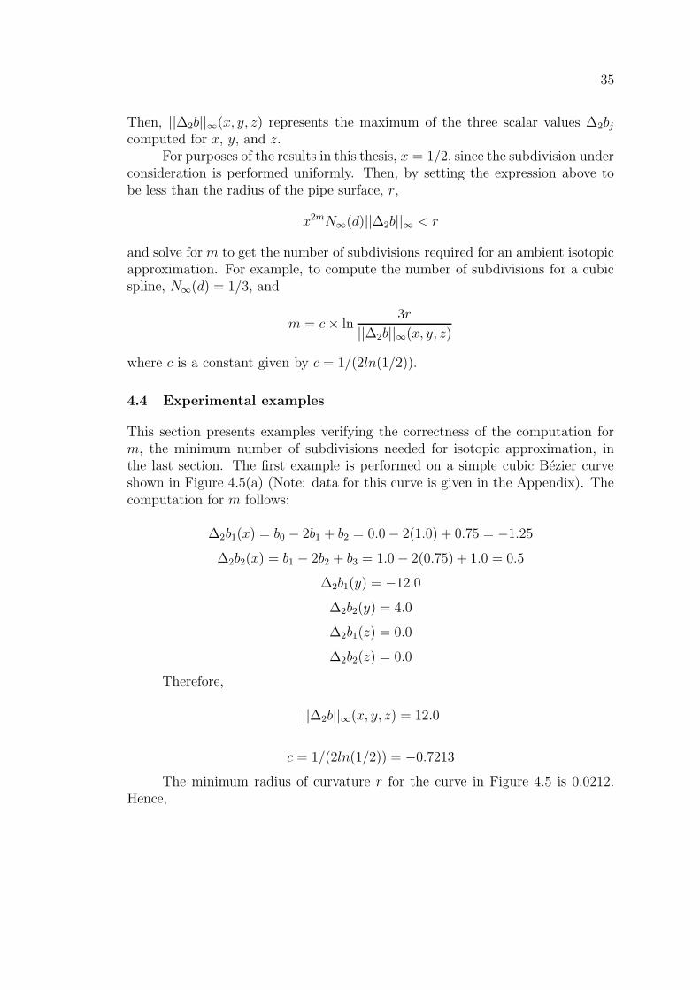
Then, ||∆2b||∞(x, y, z) represents the maximum of the three scalar values ∆2bj

computed for x, y, and z.For purposes of the results in this thesis, x = 1/2, since the subdivision under

consideration is performed uniformly. Then, by setting the expression above tobe less than the radius of the pipe surface, r,

x2mN∞

(d)||∆2b||∞ < r

and solve for m to get the number of subdivisions required for an ambient isotopicapproximation. For example, to compute the number of subdivisions for a cubicspline, N

∞(d) = 1/3, and

m = c × ln3r

||∆2b||∞(x, y, z)

where c is a constant given by c = 1/(2ln(1/2)).

4.4 Experimental examples

This section presents examples verifying the correctness of the computation form, the minimum number of subdivisions needed for isotopic approximation, inthe last section. The first example is performed on a simple cubic Bezier curveshown in Figure 4.5(a) (Note: data for this curve is given in the Appendix). Thecomputation for m follows:

∆2b1(x) = b0 − 2b1 + b2 = 0.0 − 2(1.0) + 0.75 = −1.25

∆2b2(x) = b1 − 2b2 + b3 = 1.0 − 2(0.75) + 1.0 = 0.5

∆2b1(y) = −12.0

∆2b2(y) = 4.0

∆2b1(z) = 0.0

∆2b2(z) = 0.0

Therefore,

||∆2b||∞(x, y, z) = 12.0

c = 1/(2ln(1/2)) = −0.7213

The minimum radius of curvature r for the curve in Figure 4.5 is 0.0212.Hence,

36

(a) (b)

(c) (d)

Fig. 4.5: A cubic bezier curve (a) with no subdivisions (b) after 1st subdivision(c) after 2nd subdivision, and (d) control polygon of 3rd subdivisionfits inside pipe surface.

37

m = c × ln3r

||∆2b||∞(x, y, z)= (−0.7213) × ln

3(0.0212)

12.0= 3.8

A value of m = 3.8 can easily be seen visually by experimentation. Lookingagain at Figure 4.5(a), it is clear that the radius of the pipe surface for this curvewill be minimized by the minimum radius of curvature located at the top of thiscurve, which equals 0.0212. The first subdivision is depicted in Figure 4.5(b)with its new control polygon.Figure 4.5(c) and Figure 4.5(d) show the second andthird subdivisions in a ’zoomed in’ view, along with a section of the pipe surface.It is clear that the control polygon of the second subdivision in Figure 4.5(c)intersects the pipe surface at its boundary, whereas the control polygon of thethird subdivision in Figure 4.5(d) lies completely within the pipe surface. Hence,the computation for m agrees with the visual inspection.

Chapter 5

Isotopic Surface Approximation

It is well known that a crude PL approximation of a curve may result in a differentknot type, with a specific examples already shown and cited in Chapter 2. There,a crude approximation of a smooth unknot, denoted here as K1, resulted in a PLknot with 4 crossings. Similar pathologies can occur when approximating surfaces.For example, consider a pipe surface [33], denoted S, created along K1 with theradius of S chosen so that S would be non-self-intersecting [19]. Then it should beclear that an ill-advised approximation of S could result in a change of embeddingwithin R

3. Recently published constraints [38,39] establish when approximationsof 2-manifolds preserve the original isotopy class. The proofs of these theoremsestablish a tubular neighborhood in which the approximation is guaranteed to beisotopic to the original surface. For each manifold, its tubular neighborhood isexplored as a constraint within which the isotopy class of dynamically changingmolecules can be preserved.

Splines have proven to be valuable as general geometric representations formany computing applications. A spline surface is defined in terms of a finite setof control points, which need not necessarily lie on the surface.

A spline surface1 is defined [11] over the parameters s, t ∈ [0, 1]2 as

S(s, t) =

n∑

i=0

m∑

j=0

Ni,p(s)Nj,q(t)Pi,j,

where Ni,k is defined as a step function over a non-decreasing sequence of realnumbers u0, . . . , ul, known as the knots of the spline2 as

Ni,0(u) =

{

1, if ui ≤ u < ui+1,0, otherwise

(5.1)

and

1 A spline curve is defined similarly, except there is only one independent parameter, oneindexing variable and a single summation.

2 This usage is standard for splines and should not be confused with the definition of a knotas a closed curve embedded in R

3. The contexts are usually sufficiently different to preventconfusion over this shared terminology.

38

39

Ni,k(u) =u − ui

ui+k − ui

Ni,k−1(u) +ui+k+1 − u

ui+k+1 − ui+1

Ni+1,k−1(u). (5.2)

The points Pi,j are known as the control points and the Ni,k are known as the basisfunctions.

It is a standard and widely used result on splines that the spline equationscan be modified to have an increased number of control points with this processproducing sets of control points that converge to the original curve or surfaceunder the Hausdorff metric [30,37], and this refinement process is known as sub-division [11]. If m is the cardinality of the initial set of control points, then eachsubdivision doubles the number of control points. Hence, after, n subdivisions,the number of control points is m ∗ 2n. All spline surfaces considered here willbe assumed to be continuous images of [0, 1]2, so these spline surfaces will becompact.

One advantage of splines is that the control points are often used as input tohighly efficient algorithms that have desirable numerical properties. One indica-tion as to how the control points provide shape information is that, for any spline,the convex hull of the control points will contain the spline curve or surface [30,11].Hence, the investigations reported here are directed towards discovering if the setof control points could be used to form an ambient isotopic approximation of aspline surface. There has only been partial success here because, in general, onlya subset of the control points are used in constructing the PL ambient isootopicapproximation.

One result from the literature used throughout this Chapter gives specificnumeric limits on how far the vertices of a compact triangulated 2-manifold can beperturbed while preserving ambient isotopy between the original and perturbedsurfaces [8,9]. This earlier work relied upon the expensive computation of alldistances between disjoint vertices, edges and faces.

There are three recent results about approximations of curves that also mo-tivated this present work. The first result [19] constructed an ambient isotopic PLapproximation to a spline curve, but did not specifically use the control points,possibly resulting in isotopic approximations having very different shape charac-teristics from the original curve. Their proof relied upon using pipe surfaces [33]for the construction of tubular neighborhoods (See Chapter 2).

A recent paper [31] showed preservation of an important topological prop-erty between any non-self-intersecting Bezier curve and an approximating PLcurve formed on its control points, as generated after finitely many subdivisions.These Bezier curves form a subclass of the spline curves. It was shown that aftersufficiently many subdivisions, all further subdvisions continue to yield these non-self-intersecting PL approximants over the control points, where all the controlpoints were used in forming the approximant. This then shows that the curvesare homeomorphic, but not necessarily isotopic. This result relied upon the use

40

of another aspect of spline curves, known as the hodograph [11], for which thereis no known generalization for surfaces.

In Chapter 4 it was shown that a PL curve can be created on the controlpoints that is ambient isotopic to the original curve, but this proof relied uponthe ability to discern whether a closed PL curve was unknotted. The recognitionof the unknot is a problem of considerable continuing theoretical interest [40–42],where the development of practical algorithms has remained elusive.

5.1 Isotopy of a surface by control points

While the results presented here for surfaces are similar in spirit to those cited inChapter 4 for curves, there are critical differences between curves and surfaces toemphasize. For any set of points on an oriented curve there is a natural orderingof the points defined by choosing an initial point and a faithful indexing of theremaining points by the order in which they are encountered relative to increasingarclength along the curve. If one takes the control points of a curve in order, thenthey form a polyline, or another curve. However, sample points of a surface haveno obvious order. Furthermore, if one takes the control points of a surface andconnects them by line segments (where the vertices are lexigraphically orderedrelative to their spline subscripts) one has only a net of control points, not asurface. So, any notion of isotopy between a surface and its control points mustexplicate what surface (typically a PL one) is being represented by the controlpoints. Specifically for spline curves, the technical tool of the hodograph wasused [31], but there is no obvious generalization of hodographs to surfaces.

Hence, the techniques employed here will differ from those provided forcurves. Note, however, the fact that the control net of a surface is not itselfa surface, permits the avoidance of dependency upon isotopy class recognitiontechniques, that arose in approximating a curve.

Lemma 5.1.1: Let F be a spline surface and let T (F ) be any triangulation of Fthat is ambient isotopic to F . Then there exists an ambient isotopic PL approx-imation of F , where all the points of this PL approximation are control points ofsome subdivision of F .

Proof: For T (F ), there exists a constant ν(T (F )) > 0 such that any perturba-tion of the vertices of T (F ) that is strictly less than ν(T (F ))/2 is ambient isotopicto T (F ), where the ambient isotopy has compact support [8]. For the n-th sub-division of F , let Dn denote its set of control points. Choose some ε > 0 withε < ν(T (F ))/2. Then by the convergence of subdivision [30,11] there exists somen ≥ 0 such that for each point of T (F ) there is a point of Dn within ε of T (F ).Note that this relies upon the fact that each vertex of T (F ) is also a point of F .Choose a subset Dn such that |T (F )| = |Dn| and such that each point of T (F ) has

41

a unique nearest point in Dn (If there are ties for nearest points, then these tiescan be broken by arbitrarily choosing any one of these nearest neighbors in Dn forany particular point of T (F ).) Then create a triangulation with the points of Dn

by perturbing each point of T (F ) to its nearest neighbor in Dn while maintain-ing all the same connectivity relations that existed within T (F ). Call this newlyperturbed triangulated surface T (Dn). The sets T (F ) and T (Dn) are ambientisotopic [8]. Since ambient isotopy is an equivalence relation, T (Dn) is ambientisotopic to F .

This is an “existence” proof dependent upon the a priori existence of atriangulation isotopic to F . However, previous work [18] allows the creation ofsuch a triangulation T (F ), as discussed below. While there are many results abouttriangulations of manifolds, the specific one quoted in the proof is of computationalinterest because it has both a practical algorithm and implemented software toproduce an ambient isotopic PL approximation, under the additional hypothesisthat F is orientable.

Theorem 5.1.1: For any compact C2, orientable manifold F without boundary,a sufficiently dense set of sample points can be chosen to produce a triangulationof F that is ambient isotopic to F .

Proof: This result has previously appeared in the literature [18].

The previously published result [18] relies on the Power Crust with a sam-pling criterion for F based upon local and adaptive bounds on the distance of Ffrom its medial axis MA(F ). The primary advantage of the reliance upon themedial axis is that the sampling criterion is adaptive, meaning that local choicesresult in a smaller sampling set than if a more restrictive global criterion wereused. However, this dependence upon MA(F ) remains problematic for any re-sponsive algorithm because the inherent difficulties of computing the medial axishas been expressed in the literature [43–46]. In order to avoid these medial axisalgorithmic difficulties, the work [39] establishes a global positive value ρ for atubular neighborhood about F . An advantage of using this value of ρ is thatρ can be computed from splines without ever computing any approximation ofMA(F ), while the disadvantage of any global sampling criterion is that it willusually require more sample points than an adaptive criterion.Note: The above proof can be specialized to spline curves, to show that there isan ambient isotopy between a curve formed from a subset of the control points ofsome subdivision and the original curve, without any reliance upon the hodograph.This application to spline curves is more general than a previously quoted curveresult [31] on Bezier curves, but this generalization is gained at the cost of possiblynow only using a subset of the control points obtained under subdivision.

42

5.2 Manifolds with Boundary

The previous arguments [18] were restricted to manifolds without boundary. Toconsider manifolds with boundary, theory from emerging work [47,48] will be used.The arguments are similar in spirit to those given for the proof of Lemma 5.1.1,but there is more technical subtlety required, both because of the existence of theboundary and because the known PL approximation which is ambient isotopic toF is no longer a triangulation of F .

A summary of those emerging results [47,48] is now provided, which willbe important to the proof given below. Those works show that for any compactorientable C2 manifold, M , with boundary, there exists an embedding, h from Minto a tubular neighborhood of M . The boundary of this tubular neighborhoodis also shown to always be within Hausdorff distance ρ from M , where ρ is apositive constant determined from geometric properties of M . Then, it is shownthat for any γ ∈ (0, ρ), there exists an ambient isotopic approximation N of M ,such that for each p ∈ M , there exists q ∈ N , with d(p, q) < γ and N is asubset of a triangulated manifold, T , embedded in R

3. If G is the ambient isotopyG : R

3 × [0, 1] → R3 such that G(M, 1) = N , then the image of each point x of M

is specifically given by the ‘nearest point mapping’, α : M → T , which is definedas follows. For x ∈ M , denote the normal of x by nx, chosen so that all nx’sare consistentlyoriented on M . Then α(x) is given as the point in nx ∩ T thathas the smallest distance to x. This work notes that N need not be PL, becausethe boundary of N need not be PL. However, it does show that there exists anambient isotopic PL approximation N of N that can be made arbitrarily close toN .

In addition to the notation of the previous paragraph, the following willbe invoked within the proof of the next theorem. For any set A, let |A| denotethe cardinality of A; for any function f between two sets X and Y and for anyy ∈ Y , let f←(y) = {x ∈ X : f(x) = y}; for any two points x, y ∈ R

3, letd(x, y) denote the usual Euclidean distance; for any compact subsets A, B ⊂ R

3,let dH(A, B) denote the Hausdorff distance between sets A and B; for any r > 0and any point x ∈ R

3, let Br(x) denote the open ball of radius r about x; for any2 points x, y ∈ R

3, let [x, y] denote the corresponding 1-simplex; for any 3 pointsx, y, z ∈ R

3, let [x, y, z] denote the corresponding 2-simplex.

Theorem 5.2.1: For any C2, spline surface F with boundary, there exists anambient isotopic PL approximation of F , where all the points of this PL approxi-mation are control points of some subdivision of F .

Proof: For the spline surface F , let N be its PL ambient isotopic approximationsuch that d(N, F ) < γ < ρ, where γ and ρ are as defined, above. Let the verticesof N be denoted by p0, p1, . . . , pn. Then, there exists a constant ν(N) such that

43

any perturbation of the points of N by less than ν(N)/2 results in an ambientisotopic PL approximation [8] of N . Then, for the ensuing comparisons, chooseε > 0 such that ε < min {γ, ν(N)/2}.

Using [47,48] as discussed above, for each i = 1, . . . , n, choose a unique pointpi ∈ N such that d(pi, pi) < ε/2. Now choose δ > 0, such that, for i = 1, . . . , n,

Bδ(α←(pi)) ∩ Bδ(α

←(pj)) = ∅, ∀j 6= i,

and there exists some m > 0 such that the m-th subdivision of F has a set ofcontrol points Dm, so that ∀i, ∃qi with

qi ∈ Dm ∩ Bδ(α←(pi))

such thatd(pi, β(qi)) < ε/2,

where β is defined as a function on the qi’s in the following manner:

• for each qi, determine its unique nearest point qi on F , where the existenceand uniqueness of qi is assured [47,48], because qi is in the open tubularneighborhood of radius γ about F ,

• each qi then lies on the normal nqiand β(qi) is then taken as the point

of nqi∩ N that has the smallest distance to qi, where the intersection is

guaranteed to be non-empty because of the definition of N .

Then, by the Triangle Inequality, it is clear that

d(pi, β(qi)) ≤ d(pi, pi) + d(pi, β(qi)) < 2(ε/2) = ε.

However, ε was chosen so that perturbing the vertices pi of N into the β(qi)’sresults in a new PL manifold, denoted as Tβ such that N and Tβ are ambientisotopic (and the isotopy has compact support) [8]. However, since N was alreadyambient isotopic to F (with a compact set of support), it follows that F and Tβ

are ambient isotopic over a set of compact support.Consider now, the 2-complex C formed over the qi’s by defining a 1-simplex

[qi, qj] for i, j = 1, . . . , n, with i 6= j if and only if [pi, pj] is a 1-simplex of N andsimilarly by defining a 2-simplex [qi, qj, qk] for i, j, k = 1, . . . , n, with i, j and kdistinct, if and only if [pi, pj, pk] is a 2-simplex of N . Then C is ambient isotopicto Tβ, as can be seen from the definition of β.

Hence, C and F are ambient isotopic, where C is a PL manifold formedfrom some control points of a subdivision of F .

Remark: While control points are used to develop the triangulation, it is clearlypossible that only a subset of those from a particular subdivision will be used. So,while this may provide more shape similarity than just by using points sampledfrom the surface, the trade-offs here warrant further experimental investigation.The details of the number of subdivisions needed also remain as a subject forfurther study.

Chapter 6

Algorithms

6.1 Isotopic curve subdivision algorithm

As a direct result of the Theorem 4.2.1, an experimental implementation hasbeen made to demonstrate ambient isotopic curve approximations by repeatedsubdivision. The pseudocode for the primary algorithm follows here.

Isotopic Curve Subdivision Algorithm

Input: B as defined in Theorem 4.2.1.1. Compute r for B, as defined previousls [19].2. Subdivide B until its control polygon is in Nr(B).

Output: The final control polygon – which is ambientisotopic to the original spline.

6.2 Star algorithm

Simplicial 1-complexes, considered as PL embeddings in R3, are used in CAGD to

define meshes and in CAMD to represent molecules. For simulations, it is desir-able to modify the position of individual vertices, while preserving the topologyof the complex. Large models may have in excess of ten thousand vertices, so per-formance considerations are crucial in designing simulation software, particularlyversus global constraints previously presented [8,20]. Hence, a new approach isproposed that offers more efficient sufficient conditions. This approach perturbsonly a single vertex inside a local bounding box, and then performs a check toguarantee an ambient isotopy via that bounding box.

An algorithm for locally perturbing the vertices of a 1-complex, while pre-serving the topology, is given here followed by a brief description.

44

45

Star Algorithm

Input: v ∈ K1. Compute Star(v); (See Figure 6.1(a))2. Move v to v∗ by a push [36];3. Compute Star(v∗); (See Figure 6.1(b)4. Compute B = BoundingBox(Star(v) ∪ Star(v∗));5. If B ∩ (K − Star(v)) = ∅

return true;elsereturn false;

The input to the star algorithm is the position of a single vertex, v, in theentire 1-complex, K. The collection of edges connected to v is called Star(v), andStar(v∗) is the collection of edges connected to v∗, the new position of v. Theessential characteristic of a push is that v can only be perturbed strictly less thanmin{d(vi, vj), d(vi, [vj, vk])}, ∀vi, vj, vk ∈ Star(v) such that vj, vk 6= v, vi 6= vj,and vi /∈ [vj, vk]. The bounding box, B, of Star(v) ∪ Star(v∗), is a rectilinearparallelepiped with vertices defined by the minimum values of x, y, and z and themaximum values of x, y, and z taken from the vertices of all the edges given inStar(v)∪Star(v∗). Now, if any edges of K not in Star(v) are contained in B, thenfurther testing must be performed to ensure that there are no intersecting edgesof B. Otherwise, the movement from v to v∗ is permissible, as the perturbationsare merely linear mappings.

(a) (b)

Fig. 6.1: (a) Star(v) (b) Star(v*)

46

6.3 Applications

The Isotopic Curve Subdivision Algorithm can be integrated with any availableeffective subdivision code to yield subdivisions that are ambient isotopic to curvessatisfying the hypotheses of Theorem 4.2.1. This can then be used for graphicsand engineering approximations, where fidelity to topological form is crucial.

The Star Algorithm only directly deals with 1-complexes. An experimentalpath, though, is to use this as a first approximation in simulations with geomet-ric objects formed from spline curves or surfaces. This appears to be especiallypromising with respect to simulations on high performance computing (HPC),and this algorithm has been fundamental in initiating a collaboration with IBMfor their HPC architecture of Blue Gene. The additional theory contained hereprovides some opportunities for moving beyond these 1-complexes into complexesformed with curves and surfaces. However, the execution and reporting of thoseexperiments is beyond the scope of the current dissertation and will be reportedin the future.

Chapter 7

Conclusion

The main theoretical results of this dissertation are

• demonstration that there is a large class of unknotted curves with knottedcontrol polygons (Chapter 3),

• the theory proving that iterative subdivision of non-self-intersecting Beziercurves of less than degree 5 will produce ambient isotopic control polygons,with a specific a priori bound on the number of iterations required (Chapter4),

• the theory for ambient approximation of spline surfaces by using a subset ofthe control points generated under repeated subdivision (Chapter 5), and

• pseudocode for practical algorithms and applications (Chapter 6).

In summary, these are viewed as effective contributions to the growing bodyof knowledge on incorporation of topological considerations into geometric ap-proximation algorithms. There remain some interesting opportunities to explore,particulary with respect to

• approximation of Bezier curves of degree higher than 5 (Chapter 4),

• approximation of surfaces (Chapter 5), and

• applications to scientific visualization for HPC (Chapter 6).

47

Bibliography

[1] Munkres, J. R., 1999. Topology, 2nd Edition. Prentice Hall.

[2] O’Rourke, J., 1998. Computational Geometry in C, 2 ed. Cambridge.

[3] Mantyla, M., 1983. Computational topology: a study on topological manipula-tions and interrogations in computer graphics and geometric modeling. PhDthesis, Finnish Academy of Technical Sciences, Helsinki. Acta PolytechnicaScandinavica, Mathematics and Computer Science Series 37.

[4] et. al., D. E., 1999. Emerging challenges in computational topology.http://arxiv.org/abs/cs.CG/9909001, June. Report from the NSF-fundedWorkshop on Computational Topology, Miami Beach, FL.

[5] Adams, C. C., 2001. The Knot Book: An Elementary Introduction to theMathematical Theory of Knots. W. H. Freeman and Company.

[6] Rolfsen, D., 2003. Knots and Links. AMS Chelsea Publishing, Providence,RI.

[7] Sinden, R. R., 1994. DNA Structure and Function. Academic Press.

[8] Andersson, L.-E., Dorney, S. M., Peters, T. J., and Stewart, N. F., 1995.“Polyhedral perturbations that preserve topological form”. CAGD, 12 ,pp. 785–799.

[9] T. J. Peters, e. a., 1996. “Propagating topological tolerances for rapid pro-totyping”. In MED-Vol. 4, 1996 ASME IMECE Conference Proceedings,pp. 487–498.

[10] Farouki, R. T., 1999. “Closing the gap between cad model and downstreamapplication”. SIAM News, 32 (5) June .

[11] Piegl, L., and Tiller, W., 1997. The NURBS Book, 2nd ed. Springer.

[12] Sederberg, T. W., 1983. Implicit and Parametric Curves and Surfaces forComputer Aided Geometric Design. PhD thesis, Purdue University.

48

49

[13] Hoffman, C. M., 1989. Geometric and Solid Modeling: An Introduction.Morgan Kaufman.

[14] Weiler, K., 1985. “Edge-based data structures for solid modeling in curvedsurface environments”. Computer Graphics and Applications, 5 (1) , pp. 21–40.

[15] Requicha, A. G., 1999. “Representations for rigid solids: theory, methodsand systems”. ACM Computing Surveys, 46 , pp. 185–211.

[16] Voelcker, H. B., and Requicha, A. A. G., 1977. “Geometric modelling ofmechanical parts and processes”. IEEE Computer, 10 (12) , pp. 48–57.

[17] Tilove, R. B., and Requicha, A. A. G., 1980. “Closure of boolean operationson geometric entities”. CAD, 12 (5) .

[18] Amenta, N., Peters, T. J., and Russell, A. C., 2003. “Computational topol-ogy: ambient isotipic approcimation of 2-manifolds”. Theoretical ComputerScience, 305 , pp. 3–15.

[19] Maekawa, T., Patrikalakis, N. M., Sakkalis, T., and Yu, G., 1998. “Analysisand applications of pipe surfaces”. Computer Aided Geometric Design, 15 ,pp. 437–458.

[20] Andersson, L.-E., Peters, T. J., and Stewart, N. F., 2000. “Equivalence oftopological form for curvilinear geometric objects”. International Journal ofComputational Geometry and Applications, 10 (6) , pp. 609–622.

[21] Pippenger, N., Hass, J., and Lagarias, J. C., 1999. “The computationalcomplexity of knot and link problems”. Journal of the ACM, 46 , pp. 185–211.

[22] Gilbert, N. D., and Porter, T., 1994. Knots and Surfaces. Oxford SciencePublications.

[23] Lickorish, R. W. B., 1997. An Introduction to Knot Theory. Springer-Verlag,New York.

[24] Alexander, J. W., 1928. “Topological invariants of knots and links”. Trans-actions of the American Mathematical Society, 30 , pp. 275–306.

[25] Jones, V. F. R., 1985. “A polynomial invariant for knots and links via vonneumann algebras”. Bulletins of the American Mathematical Society, 12 ,pp. 103–111.

50

[26] Liang, C., and Mislow, K., 1995. “Topological features in proteins: knotsand links”. Journal of the American Chemical Society, 117 , pp. 4201–4213.

[27] Sumners, D. W., 1995. “Lifting the curtain: Using topology to probe thehidden action of enzymes”. Notices of the AMS, 42 (5) May , pp. 528–537.

[28] Wasserman, S. A., Dungan, J. M., and Cossarelli, N. R., 1985. “Discovery ofa predicted dna knot substantiates a model for site-specific recombination”.Science, 229 , pp. 171–174.

[29] Flapan, E., 2000. When Topology Meets Chemistry: A Topological Look AtMolecular Chirality. Cambridge University Press.

[30] Cohen, E., Lyche, T., and Riesenfeld, R. F., 1980. “Discrete b-splinesand subdivision techniques in computer-aided geometric design”. ComputerGraphics and Image Processing, 14 , pp. 87–111.

[31] Neagu, M., Calcoen, E., and Lacolle, B., 2000. “Bezier curves: Topologicalconvergence of the control polygon”. In Mathematical Methods in CAGD:Oslo 2000, T. Lyche and L. L. Schumaker, Eds., Vanderbilt University Press,pp. 347–354.

[32] Farin, G., 1990. Curves and Surfaces for Computer Aided Geometric Design:A Practicle Guide, 2 ed. Academic Press, San Diego, CA.

[33] Monge, G., 1850. Application de l’Analys a la Geometrie. Bachelier, Paris.

[34] Maekawa, T., and Patrikalakis, N. M., 2002. Shape Interrogation for Com-puter Aided Design and Manufacturing. Springer, New York.

[35] Willard, S., 2001. General Topology. Addison-Wesley Publishing Company,Reading, MA.

[36] Bing, R. H., 1983. The Geometric Topology of 3-Manifolds, vol. 40. Ameri-can Mathematical Society Colloquium Publications, American MathematicalSociety, Providence, RI.

[37] Nairn, D., Peters, J., and Lutterkort, D., 1999. “Sharp, quantitative boundson the distance between a polynomial piece and its bezier control polygon”.Computer Aided Geometric Design, 16 , pp. 613–631.

[38] Sakkalis, T., and Peters, T. J., 2003. “Ambient isotopic approximations forsurface reconstruction and interval solids”. In Proceedings of the Eighth ACMSymposium on Solid Modeling and Applications, G. Elber and V. Shapiro,Eds., ACM, ACM, pp. 176–184.

51

[39] Sakkalis, T., Peters, T. J., and Bisceglio, J., 2004. “Application of ambi-ent isotopy to surface approximation and interval solids”. Computer AidedGeometric Design, 36 (11) , pp. 1089–1100.

[40] Birman, J. S., and Hirsch, M. D., 1998. “A new algorithm for recognizingthe unknot”. Geometry and Topology, 2 , pp. 175–220.

[41] Haken, W., 1961. “Theorie der normalflachen”. Acta. Math, 105 , pp. 245–375.

[42] Hass, J., Lagarias, J. C., and Pippenger, N., 1999. “The computationalcomplexity of knot and link problems”. Journal of the ACM, 46 (2) , pp. 185–211.

[43] Culver, T., Keyser, J., and Manocha, D., 2004. “Exact computation of amedial axis of a polyhedron”. Computer Aided Geometric Design, 21 (1) ,pp. 65 – 98.

[44] Damon, J., 2003. “On the smoothness and geometry of boundaries associatedto skeletal structures, i: sufficient conditions for smoothness”. Annales Inst.Fourier, 53 , pp. 1941 – 1985.

[45] Damon, J., 2004. Smoothness and geometry of boundaries associated toskeletal structures, ii: geometry in the blum case. pre-print.

[46] Damon, J., 2004. Determining the geometry of boundaries of objects frommedial data. pre-print.

[47] Abe, K., Bisceglio, J., Peters, T. J., Russell, A. C., Ferguson, D. R., andSakkalis, T., 2005. “Computational topology for reconstruction of surfaceswith boundary: integrating experiments and theory”. In International Con-ference of Shape Modeling and Applications, M. Spagnuolo, A. Pasko, andA. Belyaev, Eds., IEEE, IEEE Computer Society, pp. 288–297.

[48] et al, K. A., 2005. Computational topology for reconstructionof surfaces with boundary, part ii: mathematical foundations.www.cse.uconn.edu/~tpeters, May. pre-print.