computational simulation and analytical … · buckling resistant steel plate shear wall (br-spsw)...

COMPUTATIONAL SIMULATION AND ANALYTICAL DEVELOPMENT OF

BUCKLING RESISTANT STEEL PLATE SHEAR WALL (BR-SPSW)

Abhilasha Maurya

Thesis submitted to the faculty of the Virginia Polytechnic Institute and State University in

partial fulfillment of the requirements for the degree of

Master of Science

In

Department of Civil and Environmental Engineering

Matthew R. Eatherton, Committee Chair

Cristopher D. Moen

Carin L. Roberts-Wollmann

August 06, 2012

Blacksburg, Virginia

Keywords: Steel Plate Shear Wall, hysteretic damping, plate buckling, seismic behavior, finite

element modeling

COMPUTATIONAL SIMULATION AND ANALYTICAL DEVELOPMENT OF


Abhilasha Maurya

ABSTRACT

Steel plate shear walls (SPSWs) are an attractive option for lateral load resisting systems for both

new and retrofit construction. They, however, present various challenges that can result in very

thin web plates and excessively large boundary elements with moment connections, neither of

which is economically desirable. Moreover, SPSW also suffers from buckling at small loads

which results in highly pinched hysteretic behavior, low stiffness, and limited energy dissipation.

To mitigate these shortcomings, a new type of SPSW has been developed and investigated. The

buckling resistant steel plate shear wall (BR-SPSW) utilizes a unique pattern of cut-outs to

reduce buckling. Also, it allows the use of simple shear beam-column connections and lends

tunability to the shear wall system. A brief discussion of the concept behind the BR-SPSW is

presented. A detailed parametric study is presented that investigates the sensitivity of the local

and global system behavior to the geometric design variables using finite element models as the

main tool. The key output parameters which define the system response are discussed in detail.

Analytical solutions for some output parameters like strength and stiffness have been derived and

resulting equations are proposed. Finally, preliminary suggestions have been made about how

this system can be implemented in practice to improve the seismic resistance of the buildings.

The proposed BR-SPSW system was found to exhibit relatively fuller hysteretic behavior with

high resistance during the load reversals, without the use of moment connections.

iii

ACKNOWLEDGEMENTS

The two years which I have spent at Virginia Tech has been truly nourishing. My experiences

have enriched me socially, professionally, and intellectually, and I am grateful to have the

opportunity to acknowledge the people and organizations who have contributed to all aspects of

my life.

First and foremost, I would like to thank my advisor, Dr. Matthew R. Eatherton for the valuable

guidance and advice. Under his influence, I have grown as an engineer, researcher, and technical

writer. I would also like to thank Dr. Christopher Moen and Dr. Carin L.Roberts-Wollmann for

their invaluable support and feedback as my advisory committee.

The entire Structures group at Virginia Tech has been a tremendous resource for me. I am

grateful for the research discussions within and beyond my research group and for the thorough

and high quality lectures that the faculty provides.

My tuition and research were funded in part by the American Institute of Steel Construction

(AISC) Milek Faculty Fellowship. This support is sincerely appreciated.

Finally, and most importantly, I’d like to thank my parents, roommates and wonderful friends

who have supported me throughout my graduate studies. I am indebted to you all for the

completion of this thesis.

iv

TABLE OF CONTENTS

Abstract .......................................................................................................................................... ii

Acknowledgements ...................................................................................................................... iii

Table of Contents ......................................................................................................................... iv

List of Figures ............................................................................................................................. viii

List of Tables ............................................................................................................................... xii

Chapter 1

Introduction ................................................................................................................................... 1

1.1. Motivation for the study ....................................................................................................... 1

1.2. Objectives and scope ............................................................................................................ 4

1.3. Organization of the thesis ..................................................................................................... 6

Chapter 2

Literature Review ......................................................................................................................... 8

2.1. Solid panels .......................................................................................................................... 8

2.1.1. Solid panel with normal strength steel .......................................................................... 8

2.1.2. Solid panel with Low Yield Strength (LYS) steel ....................................................... 17

2.2. Panel with corrugated plates .............................................................................................. 19

2.3. Perforated steel plate shear walls ....................................................................................... 20

2.4. Panel with quarter-circle cutouts ........................................................................................ 22

2.5. Slit steel plate shear walls and related shear fuse plates .................................................... 23

2.5.1. Panel with rectangular slits .......................................................................................... 23

2.5.2. Rectangular fuse with buckling restrained channels ................................................... 28

2.6. Butterflyfuse ....................................................................................................................... 29

2.6.1. Panels with butterfly fuse ............................................................................................ 29

2.6.2. Panels with butterfly fuse attached to a backing plate ................................................. 30

2.7. Dissipative devices employing the ring-link system .......................................................... 31

Chapter 3

Buckling resistant steel plate shear wall (BR-SPSW) concept................................................ 35

v

Chapter 4

Validation of the BR-SPSW concept and preliminary investigations .................................... 39

4.1. Single story, one bay panel: Aligned-ring model ............................................................... 41

4.1.1. Modeling features and parameters ............................................................................... 41

4.1.2. Analysis Results .......................................................................................................... 43

4.2. Single story, one-bay panel: Influence of diameter of the rings ........................................ 45

4.3. UNCONSTRAINED RING MODEL ................................................................................ 47

4.3.1. Shell Model.................................................................................................................. 47

4.3.2. Beam Model ................................................................................................................ 49

4.4. Constrained ring model ...................................................................................................... 50

4.5. Single story, one bay panel: Staggered configuration ........................................................ 52

4.6. Summary of analysis results ............................................................................................... 53

Chapter 5

Strength calculation: Discussion of mechanisms ..................................................................... 56

5.1. Mechanism-I....................................................................................................................... 56

5.1.1. Plastic mechanism (without axial effects) ................................................................... 57

5.1.2. Plastic mechanism with axial effects ........................................................................... 60

5.2. Mechanism-II ..................................................................................................................... 64

5.2.1. Lower-Bound Solution ................................................................................................ 66

5.2.2. Upper-Bound Solution ................................................................................................. 66

5.3. Mechanism-III .................................................................................................................... 68

5.4. Mechanism-IV .................................................................................................................... 71

5.5. Comparison of results......................................................................................................... 73

Chapter 6

Stiffness calculation: Discussion of mechanisms ...................................................................... 75

6.1. Unconstrained ring model .................................................................................................. 75

6.2. Constrained ring model ...................................................................................................... 81

Chapter 7

Effect of initial imperfections ..................................................................................................... 85

7.1. Effect of magnitude of initial imperfection ........................................................................ 85

7.2. Effect of the shape of initial imperfection .......................................................................... 87

vi

Chapter 8

Parameteric study ....................................................................................................................... 91

8.1. Input parameters ................................................................................................................. 92

8.1.1. Thickness of steel plate used (t) .................................................................................. 92

8.1.2. Outer radius of the rings (Ro) ...................................................................................... 92

8.1.3. Width of the rings (Wc) ............................................................................................... 92

8.1.4. Width of the connecting link (Wl) ............................................................................... 92

8.2. Output parameters .............................................................................................................. 93

8.2.1. Strength, stiffness and yield drift ................................................................................. 93

8.2.2. Total energy dissipation............................................................................................... 94

8.2.3. Energy Dissipation Ratio ............................................................................................. 94

8.2.4 Buckling Ratio .............................................................................................................. 95

8.2.5. Length of the cut .......................................................................................................... 97

8.2.6. Openness of the wall.................................................................................................... 97

8.2.7. Peak strength................................................................................................................ 97

8.2.8. Weight ratio ................................................................................................................. 98

8.3. Test sets .............................................................................................................................. 98

8.4. Results and discussion ...................................................................................................... 101

8.4.1. Hysteretic behavior .................................................................................................... 101

8.4.2. Buckling ratio ............................................................................................................ 105

8.4.3. Trend plots ................................................................................................................. 108

8.5. Comparative analysis: SPSW and BR-SPSW .................................................................. 126

8.6. Analytical vs. Computational results ............................................................................... 127

8.6.1. Comparison of strength of the full wall ..................................................................... 128

8.6.2. Comparison of stiffness of the full wall .................................................................... 129

Chapter 9

Fracture prediction and future work ...................................................................................... 131

9.1. SMCS model .................................................................................................................... 131

9.2. CVGM model ................................................................................................................... 132

9.3. Extended finite element modeling (XFEM) ..................................................................... 136

vii

Chapter 10

Experimentational study design .............................................................................................. 140

Chapter 11

Summary and conclusions ........................................................................................................ 146

11.1. Preliminary investigations .............................................................................................. 146

11.2. Analytical solution: strength of the full wall .................................................................. 147

11.3. Analytical solution: stiffness of the full wall ................................................................. 147

11.4. Effect of initial imperfections ........................................................................................ 149

11.5. Parametric study ............................................................................................................. 149

11.6. General obeservations and conclusions.......................................................................... 151

References .................................................................................................................................. 154

Appendix A: Trend Plots.......................................................................................................... 159

Appendix B: Hysteretic Plots ................................................................................................... 167

Appendix C: Energy Dissipation Ratio ................................................................................... 176

Appendix D: Strength Calculation .......................................................................................... 185

Appendix E: Copyrighted Figures .......................................................................................... 193

viii

LIST OF FIGURES

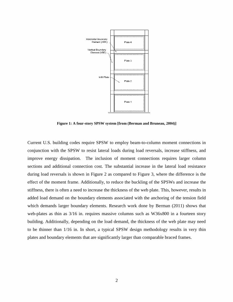
Figure 1: A four-story SPSW system [from (Berman and Bruneau, 2004)] .................................. 2

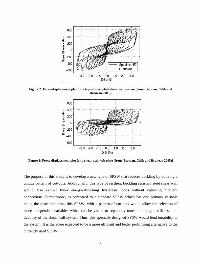
Figure 2: Force-displacement plot for a typical steel plate shear wall system [from (Berman,

Celik and Bruneau 2005)] ............................................................................................................... 3

Figure 3: Force-displacement plot for a shear wall web plate [from (Berman, Celik and Bruneau

2005)] .............................................................................................................................................. 3

Figure 4: Buckling resistant steel plate shear wall and a basic ring unit ........................................ 4

Figure 5: Diagrammatic representation of Strip Model [from (Lubell et al. 2000)]..................... 12

Figure 6: Diagrammatic representation of multi-angle strip model [from (Lubell et al. 2000)] .. 13

Figure 7: Infill panel connection details tested [from (Schumacher, Grondin and Kulak 1999)] 14

Figure 8: Test conducted by Berman and Bruneau (2005) demonstrating SPSW behavior ......... 15

Figure 9: Perforated steel plate shear walls [from (Roberts et al. 1992 and Vian et al. 2005)] .... 20

Figure 10: Steel plate walls with rectangular slits [from (Hitaka et al. 2006)] ............................. 24

Figure 11: Panel with butterfly fuse [from (Borchers, Peña, Krawinkler, and Deierlein 2010)] . 30

Figure 12: Yielding frame with constant cross-section [from (Tyler 1985)]................................ 31

Figure 13: Yielding frame with varying width [from (Ciampi and Samuelli-Ferretti 1990)] ...... 32

Figure 14: Yielding frame with varying depth [from (Ciampi and Samuelli-Ferretti 1990)] ...... 32

Figure 15: Yielding frame with complementary plates [from (Ciampi and Samuelli-Ferretti

1990)] ............................................................................................................................................ 33

Figure 16: Ring fuse [from (Rogers and Morrison 2011)] ........................................................... 34

Figure 17: Geometry of the circle and the deformed ellipse ........................................................ 35

Figure 18: Concept showing how the ring eliminates slack in the direction transverse to the

tension diagonal ............................................................................................................................ 37

Figure 19: BR-SPSW subjected to lateral load ............................................................................. 37

Figure 20: Geometric parameters of the SPSW rings ................................................................... 40

Figure 21: Modeling features of the SPSW panel ........................................................................ 41

Figure 22: Stress-strain behavior of the steel used for analysis .................................................... 42

Figure 23: Loading Protocol used in the ABAQUS analysis ....................................................... 43

Figure 24: Hysteresis curve for the single story, one-bay panel. .................................................. 44

Figure 25: One bay, one story aligned ring panel at the 2% drift ................................................. 45

Figure 26: Hysteresis curve and out-of-plane deformation for Panel 1 ........................................ 46

Figure 27: Hysteresis curve and out-of-plane deformation for Panel 2 ........................................ 47

Figure 28: Unconstrained ring model ........................................................................................... 48

Figure 29: Load-displacement relationship for unconstrained ring shell model .......................... 48

Figure 30: Comparison of effective Poisson’s ratio of the single ring unit .................................. 49

Figure 31: Beam model for unconstrained configuration ............................................................. 50

Figure 32: Force-displacement curve for unconstrained beam model .......................................... 50

Figure 33: Constrained ring model ............................................................................................... 51

Figure 34: Load-displacement curve for constrained ring model ................................................. 51

ix

Figure 35: Deformation and stress distribution of the staggered full-size panel at the end of the

test ................................................................................................................................................. 52

Figure 36: Load-drift plot for staggered full-size panel................................................................ 53

Figure 37: Pictorial Representation of Mechanism I .................................................................... 56

Figure 38: Free body diagram of quarter of a ring with radius R ................................................. 57

Figure 39: Plastic Hinge mechanism without axial effects ........................................................... 58

Figure 40: Deformation of the ring as governed by Mechanism-I without considering axial

effects ............................................................................................................................................ 59

Figure 41: Plastic mechanism with axial effects........................................................................... 60

Figure 42: axial-bending interaction curve for rectangular cross-section [from (Chen and Han

2007)] ............................................................................................................................................ 61

Figure 43: Elaborate analysis of the ring considering axial affects .............................................. 62

Figure 44: Line diagram for Mechanism -II ................................................................................. 65

Figure 45: Stress distribution in an un-constrained ring (red and orange regions are yielded) .... 65

Figure 46: Dimensional features of Mechanism-II ....................................................................... 65

Figure 47: Free body diagram of quarter of a ring (Mechanism-II) ............................................. 66

Figure 48: Development of plastic hinge in the ring as governed by Mechanism-II ................... 67

Figure 49: idealized line-diagram for Mechanism-III .................................................................. 69

Figure 50: Deformation of the ring as governed by Mechanism-III ............................................. 69

Figure 51: Deformed shape and the stress distribution of the constrained ring ABAQUS model 71

Figure 52: Deformed constrained ring represented by a quadrilateral ......................................... 71

Figure 53: The constrained ring represented in the form of a line diagram ................................. 72

Figure 54: Unconstrained ring model ........................................................................................... 75

Figure 55: Resultant stiffness of the ring ...................................................................................... 77

Figure 56: Stiffness of the full wall .............................................................................................. 78

Figure 57: Displacement of inclined arrays .................................................................................. 79

Figure 58: Line diagram of the constrained ring model ............................................................... 81

Figure 59: Arrangement of constrained ring models in the full panel .......................................... 83

Figure 60: Effect of the magnitude of initial imperfections for plate A4 ..................................... 86

Figure 61: Effect of initial imperfection for plate B11 ................................................................. 87

Figure 62: Effect of shape of initial imperfection on plate A4 ..................................................... 90

Figure 63: effect of shape of initial imperfection on plate B11 .................................................... 90

Figure 64: Loading protocol used for the parametric study .......................................................... 91

Figure 65: Strength, Stiffness and Yield Drift calculation from force-displacement plot ............ 94

Figure 66: Plot showing the method for calculating the energy dissipation ratio ........................ 95

Figure 67: Plot showing the variation of out-of-plane displacement across the width of the web

plate ............................................................................................................................................... 96

Figure 68: FFT plot for a specimen .............................................................................................. 97

Figure 69: Figure showing the dependence of hysteretic behavior on thickness for 10’’ outer ring

radius ........................................................................................................................................... 102

x

Figure 70: Figure showing the dependence of the hysteretic behavior on the ring radius (t=1/2’’)

..................................................................................................................................................... 103

Figure 71: Figure showing the dependence of the hysteretic behavior on the ring width .......... 104

Figure 72: Variation of out-of-plane deformation across the width of the web-plate ................ 107

Figure 73: Discrete Fourier Transform for Specimen A1 and A4 .............................................. 108

Figure 74: Effect of web plate thickness and radius on strength/ring ......................................... 110

Figure 75: Effect of Ro/wc and Ro/t ratios on strength/ring unit ................................................. 110

Figure 76: Effect of Ro/wl and Ro/t ratios on strength/ring unit .................................................. 111

Figure 77: Effect of web plate thickness and radius on stiffness/ring ........................................ 112

Figure 78: Effect of Ro/wc and Ro/t ratios on the stiffness/ring .................................................. 112

Figure 79: Effect of Ro/wl and Ro/t on stiffness/ring .................................................................. 113

Figure 80: Effect of thickness and radius on total dissipated energy ......................................... 114

Figure 81: Effect of Ro/t on the total dissipated energy .............................................................. 115

Figure 82: Effect of Ro/wl on total dissipated energy ................................................................. 115

Figure 83: Effect of Ro/wc on total dissipated energy ................................................................. 116

Figure 84: Effect of thickness and radius on energy dissipation ratio ........................................ 117

Figure 85: Effect of Ro/wc and Ro/t on energy dissipation ratio ................................................. 118

Figure 86: Effect of Ro/wl on energy dissipation ratio ................................................................ 118

Figure 87: Effect of radius and thickness on buckling ratio ....................................................... 119

Figure 88: Effect of wc/t on buckling ratio ................................................................................. 119

Figure 89: Effect of Ro/t on buckling ratio ................................................................................. 120

Figure 90: Effect of Ro/wc and Ro/t on buckling ratio ................................................................. 120

Figure 91: Effect of ring radius on the length of cut................................................................... 121

Figure 92: Effect of Ro/wl on the length of cut ........................................................................... 121

Figure 93: Effect of Ro/wc on the length of cut ........................................................................... 122

Figure 94: Effect of thickness and radius on yield drift .............................................................. 123

Figure 95: Effect of Ro/wc and Ro/t on yield drift ....................................................................... 123

Figure 96: Effect of wc/t on yield drift ........................................................................................ 123

Figure 97: Effect of Ro/t on yield drift ........................................................................................ 124

Figure 98: Comparison of hysteretic behavior of BR-SPSW and SPSW ................................... 127

Figure 99: Last cycles comparing the total energy dissipation for BR-SPSW and SPSW ......... 127

Figure 100: Percent error in the predicted strength as compared to the FE results .................... 128

Figure 101: Plot showing the dependence of the accuracy of the analytical solution on Ro/wl

ratio ............................................................................................................................................. 130

Figure 102: CVGM model example ........................................................................................... 134

Figure 103: Dependence of the equivalent strain to fracture on the stress triaxiality [from (Bao

and Wierzbicki 2004)] ................................................................................................................ 135

Figure 104: Initiation of crack in a single-ring model ................................................................ 137

Figure 105: Plot showing the effect of fillet radius on crack initiation ...................................... 138

Figure 106: Force-displacement curve and crack initiation location for 3in. fillet model ......... 139

xi

Figure 107: A typical test specimen to be tested as a part of experimental study ...................... 140

Figure 108: Experiment setup for small-scale BR-SPSW test .................................................... 145

Figure A.109: Trend plots for strength per ring .......................................................................... 160

Figure A.110: Trend plots for stiffness per ring ......................................................................... 161

Figure A.111: Trend plots for yield drift % ................................................................................ 162

Figure A.112: Trend plots for total dissipated energy ................................................................ 163

Figure A.113: Trend plots for energy dissipation ratio ............................................................... 164

Figure A.114: Trend plots for buckling ratio .............................................................................. 165

Figure A.115: Trend plots for cutting length .............................................................................. 166

Figure A.116: Hysteresis plots for specimens ............................................................................ 175

Figure A.117: Plots for the calculation of energy dissipation ratio ............................................ 184

Figure A.118: Plots showing the method for calculation of full wall strength ........................... 192

xii

LIST OF TABLES

Table 1: Notations for the geometric features of BR-SPSW ........................................................ 40

Table 2: Engineering and true stress and strain values used for steel ........................................... 42

Table 3: Geometrical features of the panels to test the influence of the diameter ........................ 45

Table 4: Comparison of analysis results of the rings units ........................................................... 54

Table 5: Comparison of analysis results of the full panel ............................................................. 55

Table 6: Comparison of computational and analytical results for unconstrained models ............ 74

Table 7: Comparison of computational and analytical results for constrained model .................. 74

Table 8: Comparison of computational and analytical results for full wall models ..................... 74

Table 9: Comparison of results obtained from Mechanism-IV to computational results ............. 74

Table 10: Geometric features of A4 and B11 ............................................................................... 86

Table 11: Table showing the eigen buckling modes of specimen A4 and B11 ............................ 88

Table 12: Table showing the tests done as a part of SERIES A of the parametric study ............. 99

Table 13: Table showing the tests done as a part of SERIES B of the parametric study ............. 99

Table 14: Table showing the tests done as a part of SERIES C of the parametric study ........... 100

Table 15: Table showing the tests done as a part of SERIES D of the parametric study ........... 101

Table 16: Output parameters for the test specimens of SERIES A ............................................ 124

Table 17: Output parameters for the test specimens of SERIES B............................................. 125

Table 18: Output parameters for the test specimens of SERIES C............................................. 125

Table 19: Output parameters for the test specimens of SERIES D ............................................ 126

Table 20: Predicted behavior of the experiment Specimen 1 ..................................................... 141








1

CHAPTER 1

INTRODUCTION

1.1. MOTIVATION FOR THE STUDY

Steel plate shear walls (SPSWs) have been investigated in numerous research projects, and

implemented in quite a few buildings (Sabelli and Bruneau, 2006). SPSWs designed in the U.S.

and Canada generally use thin plates that are allowed to buckle. Previous studies have shown that

SPSWs exhibit significant post-buckling capacity and energy dissipation takes place as the web

plate yields in the inclined tension field direction.

A typical steel plate shear wall (SPSW) consists of a thin steel plate, referred to as the web plate,

bounded at the sides by columns, also referred to as vertical boundary elements (VBE), and at

the floor levels by beams, also referred to as horizontal boundary elements (HBE). This

arrangement is shown in Figure 1. Web plates, adequately anchored by the boundary elements,

buckle in shear and form a diagonal tension field to resist lateral loads. The basic design process

of a SPSW requires the sizing of the web plate such that it can resist the entire base shear.

Additionally, HBEs and VBEs must be designed to elastically resist the development of the full

expected tensile capacity of the web plate to ensure that the web plate can yield in tension prior

to the plastic hinging of the boundary elements. (AISC 341-10). The force-displacement

behavior of a typical steel plate shear wall system (Berman and Bruneau, 2005) is shown in

Figure 2. The experimental setup was designed such that the boundary elements were connected

through a rigid moment connections. The hysteretic behavior shown in Figure 2 is therefore due

to the moment frame and the web plate. The hysteretic behavior is stable, but suffers substantial

pinching. This pinching in the hysteresis curve aggravates when the force-deformation behavior

of the web plate alone is considered as shown in Figure 3. This behavior is due to the fact that

the web plate acting in tension field is like tension-only bracing. Tension-only bracing is not

allowed in seismic zones because there is no lateral load resistance during load reversal which is

similar to the force-deformation behavior of the web plate (refer Figure 3). Moreover, the highly

pinched hysteretic behavior of SPSW web plate results in much lower energy dissipation. Early

buckling of the web plate also causes reduction in the wall stiffness.

2

Figure 1: A four-story SPSW system [from (Berman and Bruneau, 2004)]

Current U.S. building codes require SPSW to employ beam-to-column moment connections in

conjunction with the SPSW to resist lateral loads during load reversals, increase stiffness, and

improve energy dissipation. The inclusion of moment connections requires larger column

sections and additional connection cost. The substantial increase in the lateral load resistance

during load reversals is shown in Figure 2 as compared to Figure 3, where the difference is the

effect of the moment frame. Additionally, to reduce the buckling of the SPSWs and increase the

stiffness, there is often a need to increase the thickness of the web plate. This, however, results in

added load demand on the boundary elements associated with the anchoring of the tension field

which demands larger boundary elements. Research work done by Berman (2011) shows that

web-plates as thin as 3/16 in. requires massive columns such as W36x800 in a fourteen story

building. Additionally, depending on the load demand, the thickness of the web plate may need

to be thinner than 1/16 in. In short, a typical SPSW design methodology results in very thin

plates and boundary elements that are significantly larger than comparable braced frames.

3

Figure 2: Force-displacement plot for a typical steel plate shear wall system [from (Berman, Celik and

Bruneau 2005)]

Figure 3: Force-displacement plot for a shear wall web plate [from (Berman, Celik and Bruneau 2005)]

The purpose of this study is to develop a new type of SPSW that reduces buckling by utilizing a

unique pattern of cut-outs. Additionally, this type of resilient buckling resistant steel shear wall

would also exhibit fuller energy-absorbing hysteresis loops without requiring moment

connections. Furthermore, as compared to a standard SPSW which has one primary variable

being the plate thickness, this SPSW, with a pattern of cut-outs would allow the selection of

more independent variables which can be varied to separately tune the strength, stiffness and

ductility of the shear wall system. Thus, this specially designed SPSW would lend tunability to

the system. It is therefore expected to be a more efficient and better performing alternative to the

currently used SPSW.

4

The concept behind the resilient buckling resistant steel shear wall is to reduce the out-of plane

buckling of shear walls by exploiting a unique characteristic of the ring-type cut-outs. The basic

configuration of the buckling resistant steel plate shear wall (BR-SPSW) and the ring shaped cut-

outs, which form the basic unit of the full-wall, are shown in Figure 4. When the wall is

subjected to lateral forces, this basic ring unit deforms into an ellipse. The transverse and

longitudinal deformations of a circular ring that is being stretched into an ellipse are nearly

equal. This implies that for a SPSW made of rings, in the direction perpendicular to the tension

field, the slack in the compression diagonal direction will be removed. The removal of slack in

the compression diagonal will lead to an almost immediate development of tension field action in

the opposite direction upon load reversal. In other words, the BR-SPSW reduces buckling due to

the fact that the elongation of the ring in one radial direction will be compensated by the

shortening of the ring in the perpendicular radial direction, thus reducing out-of-plane

deformation. These concepts are further examined in Chapter 3.

Ring

Simple

Connections

Horizontal Boundary elements (HBE)

Horizontal Boundary elements (HBE)

Ver

tica

l B

oundar

y E

lem

ents

(V

BE

)

Ver

tica

l B

oundar

y E

lem

ents

(V

BE

)

Ring Unit

Link

Figure 4: Buckling resistant steel plate shear wall and a basic ring unit

1.2. OBJECTIVES AND SCOPE

The main aim of this report is to develop a more efficient and high performance shear wall

system. The concept behind BR-SPSW is new and hence should be extensively explored before

it is used for practical purposes. To achieve this goal, global and local behavior of BR-SPSW has

5

been investigated thoroughly using computational and analytical methods. Additionally, an

attempt has been made to devise means (analytical equations and trend plots) to aid the design of

BR-SPSW.

This report is organized around six objectives outlined below:

Proposing the BR-SPSW concept: Propose the idealized concept behind BR-SPSW and

how the new system will reduce buckling of the web plate as compared to a typical

SPSW system.

Preliminary investigation of the BR-SPSW concept: As mentioned previously the idea

behind BR-SPSW is new and thus requires some preliminary validation through carefully

designed models. This type of investigation is required to prove that the proposed concept

works more efficiently than a typical SPSW. This exercise also paves the way for a more

exhaustive parametric study.

Developing mathematical models for system behavior: Understanding the deformation

mechanics of the ring units in a full wall and developing analytical and empirical

solutions for major system response (strength and stiffness) needs to be done. The results

from these models must then be compared to the computational results from the

preliminary study and the parametric study to determine the efficacy of the proposed

equations.

Performing parametric study: Developing a set of computational models to study the

influence of the geometric features of the plate on the overall system response is

necessary to conduct the parametric study using ABAQUS (ABAQUS Version 6.10

Documentation) as the finite element analysis tool. Analyzing the results of the analysis

and demonstrating the system behavior using suitable plots is a major objective of this

research. The buckling behavior of the web-plate is also studied.

Understanding fracture behavior: The rings in BR-SPSW may be prone to fracture due to

their intricate shapes and reentrant corners. Methods to analyze the initiation and

propagation of cracks in the ring have therefore been investigated.

Proposing experimental program: Development of a set of experimental specimens and

test set-up for experimentation is required. The behavior of the panels needs to be

predicted using the analytical tools developed.

6

1.3. ORGANIZATION OF THE THESIS

The report is divided into eleven chapters, including this introduction, and four appendices.

Chapter 2 briefly summarizes the research work done in the field of steel plate shear walls. It

focusses on the numerous variations of SPSW that have been investigated in the past.

Additionally, some energy dissipating devices which work on similar grounds as the ring units

have been discussed in this chapter.

Chapter 3 demonstrates the idealized concept behind BR-SPSW. Mathematical tools have been

used to show how the use of ring-like cutouts in BR-SPSW help in reducing buckling.

Chapter 4 describes the preliminary investigation of the BR-SPSW concept. Four full scale

models with different configurations and ring sizes have been analyzed using ABAQUS as the

finite element analysis tool. Additionally, two ring units with different boundary conditions were

analyzed to understand the deformation behavior of the rings.

Chapter 5 focuses on understanding the deformation mechanics of the rings to develop an

analytical solution for the strength of the ring units. This solution is then translated to the

strength of the full wall.

On a similar ground as Chapter 5, Chapter 6 uses the single ring models developed in Chapter 4

to derive analytical and empirical equations for the stiffness of the full wall.

Chapter 7 investigates the effect of initial imperfections of the web-plate on the overall system

behavior. Random imperfections and imperfections in the shape of buckling modes of the web

plate were studied and necessary conclusions on the influence of initial imperfection are

presented.

Chapter 8 summarizes the parametric study done to build on the work done in Chapter 4. This

chapter tabulates the model sets carefully designed to thoroughly understand the sensitivity of

the system behavior on the geometric features of BR-SPSW followed by the detailed finite

element analysis results and conclusions.

7

Chapter 9 discusses the various techniques that can be used to predict fracture in BR-SPSW

using analytical models proposed by various researchers. This discussion is backed up by

relevant literature review. Additionally, extended FEM (XFEM) technique has been used to

model crack in a single ring model. Recommendations have been made on future work in

fracture prediction and modeling.

Chapter 10 outlines the experimental program that is being conducted at Virginia Tech to

validate the concept of BR-SPSW. A set of eight specimens have been proposed and behavior

related predictions have been made using the computational and analytical techniques developed

through the course of this research.

Chapter 11 summarizes the work presented in this report and provides a compilation of

conclusions.

8

CHAPTER 2

LITERATURE REVIEW

This chapter summarizes the previous research work done on steel plate shear walls with a focus

on system behavior obtained from previous experiments. The latter part of the section reviews

the work done on some dissipative devices also known as yielding frames which may be

considered as an inspiration for the development of buckling resistant steel plate shear walls.

2.1. SOLID PANELS

2.1.1. Solid panel with normal strength steel

Thorburn, Kulak and Montgomery (1983) recognized that thin plate shear walls have significant

post-buckling strength and developed a method of analysis on this basis. An analytical model

was designed to study the shear resistance provided by the buckled plate, wherein the tension

zone developed in a buckled plate is represented as a series of inclined planar truss members,

capable of transmitting only tension loads. This model, based on the work of Wagner (1931),

was used to investigate transfer of forces and the resulting stress redistribution in thin plate walls.

The analysis was conducted assuming that the boundary elements were stiff and allowed the

development of tension field in the web plate. The investigation of the post-buckling strength of

a panel was not done for cyclic loads. Using the analytical model, parametric studies were done

to determine the influence of column stiffness and plate thickness and aspect ratio on the overall

stiffness and strength of the shear wall panels. It was concluded that increasing web thickness

and column stiffness have positive effects on panel shear capacity. Also, panel stiffness increases

linearly as the panel length increases. It was noted that the angle of inclination of the diagonal

tension forces in a shear wall is a function of the column and beam moments of inertia, panel

dimensions and the plate thickness. Also, as column flexibility increases, variation of tensile

forces across the plate increases. Maximum stresses occur at mid-plate and they decrease

towards the plate edges. Finally, some recommendations were made to improve the analytical

model and to compare this study with experimental data.

Timler and Kulak (1983) tested a large-scale single story steel shear wall test specimen to verify

the analytical work done by Thorburn et al. (1983). The beam-to-column connection was pin-

9

jointed for exterior connections and continuous for interior connections. The 5 mm infill panel

was welded to the boundary frame by means of a 6mm thick “fish plate” The specimen was

tested under monotonically increasing loading to the serviceability drift limit, followed by the

final loading excursion until the failure of the structural system. No gravity loads were applied to

the system. The test results were then compared with the predicted results. It was noted that there

was good agreement between predicted and actual principle stresses in the plate and axial

stresses in the frame members. The angle of inclination of the principle stresses was found to be

between 46.6ᵒ and 53.2ᵒ. The predicted angle was 51.0ᵒ. Accurate prediction of the entire load-

displacement curve was obtained. However, the bending strains in the frame members were

over-estimated in each case. Thus, the analytical method put forward by Thorburn, et al. (1983)

was found to be a satisfactory approach.

Tromposch and Kulak (1987) verified the analytical model developed by Thorburn, et al. (1983),

on a specimen subjected to cyclic loading. The specimen consisted of two panels arranged so that

opposing tension fields would form. It had story height of 2200 mm, a bay width of 2750 mm

and a panel thickness of 3.25 mm. The boundary members were joined by bolted connections.

The steel panels were connected to the frame by using 5mm fish plates. The columns in the

frame were axially preloaded to simulate the effect of gravity loads. The specimen was subjected

to two loading phases: a cyclic loading phase (28 cycles) and a monotonic loading phase. During

the cyclic phase, a maximum load of 4000 kN was applied and a maximum centerline deflection

of 17 mm (0.8% drift) was reached. The hysteresis loops were stable, but pinching was observed

after 8th

cycle. The displacement ductility achieved was about 4.3 for compression cycle and 6.8

for tension cycle. Weld tearing at several corners was observed at the end of this phase. After

completing this phase, the specimen was loaded monotonically to a maximum load of 6000 kN.

The maximum deflection achieved was 71mm (3.2% drift).The axial loads measured in the

frame members produced a good correlation with those predicted by the inclined tension bar

model. The measured orientation of the principal strains was close to the predicted value of

44.0ᵒ. It was noted that hysteretic behavior of an unstiffened steel plate can be predicted with a

reasonable accuracy by the analytical method proposed by Thorburn, et al (1983). It was also

recommended that welds between the panel and the boundary members should be designed to

carry the ultimate design capacity of the plate material. Finally, it was concluded that inclined

10

tension model bar can be used with confidence to evaluate the strength and capacity of the steel

plate shear wall.

Cassese et al. (1993) investigated the seismic behavior of unstiffened thin steel- plate shear

walls. The main aim of the research was to assess the feasibility of thin plate shear walls and to

develop new design methods to result in more optimal designs. Eight quarter-scale single-bay

three-story specimens were tested. These specimens varied in the beam-to-column connections

(moment and shear connections). Three plate thicknesses (gage 22, 14 and 12) were used. The

infill plates were welded to the frame elements. One of the specimens used was just a frame

without any infill plate. The test results showed that as compared to the frame with no plates, the

specimen with gage 22 plate (0.76 mm thickness) was initially nine times stiffer. The thickening

of the plates did not result in a substantial increase in the stiffness. With respect to the strength of

the plate, it was found that thinnest plate shear wall (gage 22) was 2.8 times stronger than frame

with no infill plate. Also, a two-fold increase in strength is observed when a specimen with gage

22 plates is compared with gage 14 plate (1.87 mm thickness). It was also noted that in slender

specimens, the plate yielded long before inelastic behavior is observed in the column which is a

desirable characteristics. As anticipated, in thicker plates failure was governed by inelastic

instability of the column. It was observed that the beam-to-column connection did not have a

major effect on the frame behavior. However, this observation was attributed to the fact that the

plates are continuously welded to the frame elements so the beam-to-column connection ended

up behaving like a moment connection, even when the beam flanges were not welded to the

column flanges. However, for more slender members, moment connections have positive effect

on initial stiffness and strength. Lastly, energy dissipation of the thicker specimen was found to

be almost 2.5 times that of the slender specimen.

Elgaaly (1998) performed a series of tests on thin steel plate shear walls under cyclic loading. An

analytical model to determine the behavior of the shear walls was also presented. The model was

capable of predicting the behavior for plates with both welded and bolted connection. The tests

were conducted in two phases. Eight quarter scale single bay three story specimens were tested

in Phase I. These specimens varied in the beam-to-column connections (moment and shear

connections) and plate thickness. The plate-to-frame connection was welded in nature for all the

specimens. A detailed summary of results and conclusions for Phase 1 tests has been presented in

11

a paper by Caccese et al. (1993). Phase II tests were performed on seven one third scale single

bay two story specimen. Gage 13 (0.0897 in.) plates were used in these tests and the plate-to-

beam connection was bolted in all the specimens except one. The columns in all the elements

except for one were subjected to compressive axial force. Shear connection detailing was done

between the beam and the column of the frame. Also, the bolt spacings were varied in the

specimen to determine the optimum bolt spacing. Most of the tests in Phase II had to be stopped

prematurely due to either buckling of the column or connection failure. The specimen tested with

all the planned cycles reached a drift of 2.39%. A number of conclusions were drawn from Phase

II tests. Firstly, it was concluded that bolt spacing did not affect the mode of failure. Also, it was

noted that absence of column axial compressive loads does not change the behavior of the wall

substantially. The author has recommended that the columns of the bay should be strong enough

to allow the plate panels to develop full tension fields and yield without any premature failure of

the columns. It was also concluded from the tests that welded plates exhibited higher elastic

stiffness and initial yielding load compared to the bolted specimens. However, the ultimate

capacity of welded and bolted walls is comparable. One of the most significant contributions

from this work is the development of an analytical model using equivalent truss elements which

is able to depict the test results to a good degree of accuracy.

Lubell, Prion, Ventura and Rezai (2000) studied the performance of single and multi-story

unstiffened steel shear walls subject to cyclic quasi-static loading. One four-story and two single-

story steel plate shear wall specimens were tested. Each specimen had unstiffened infill panels

having aspect ratio of 1:1 thickness of 1.5mm (gage16) and yield stress of 46 ksi (320 MPa). Full

moment connections were provided at all beam-column joints by continuous fillet-welds. For the

four-story specimen, each horizontal load was applied at each floor. Gravity loading of this

specimen was simulated by means of steel masses attached at each story level. For single story

specimens, no gravity loading was applied. It was observed that the column of the multistory

frame yielded before significant inelastic action occurred in the infill plate. Also, significant pull-

in of the columns caused by the tension field in the infill plates, resulted in an hour-glass

deformation mode of all the specimens. It is therefore recommended as a necessary step that

capacity design of the bounding columns in a steel plate shear wall is done to ensure that the

infill panels yield prior to column hinging and to minimize pull-in of the columns. It was also

noted that flexurally stiff beams at the top and bottom of the shear wall are important to prevent

12

the formation of plastic hinges and to avoid the decrease of out-of-plane stability of the frame.

Further, it was observed that the multi-story specimen was more flexible that the single-story

specimen because the influence of the overturning moment is more significant as the height of

the structure increases. A series of numerical models using strip models was employed to

validate the results of the experiments and in all cases the results obtained were fairly accurate

with the exception that the elastic stiffnesses of the single story specimens were over predicted

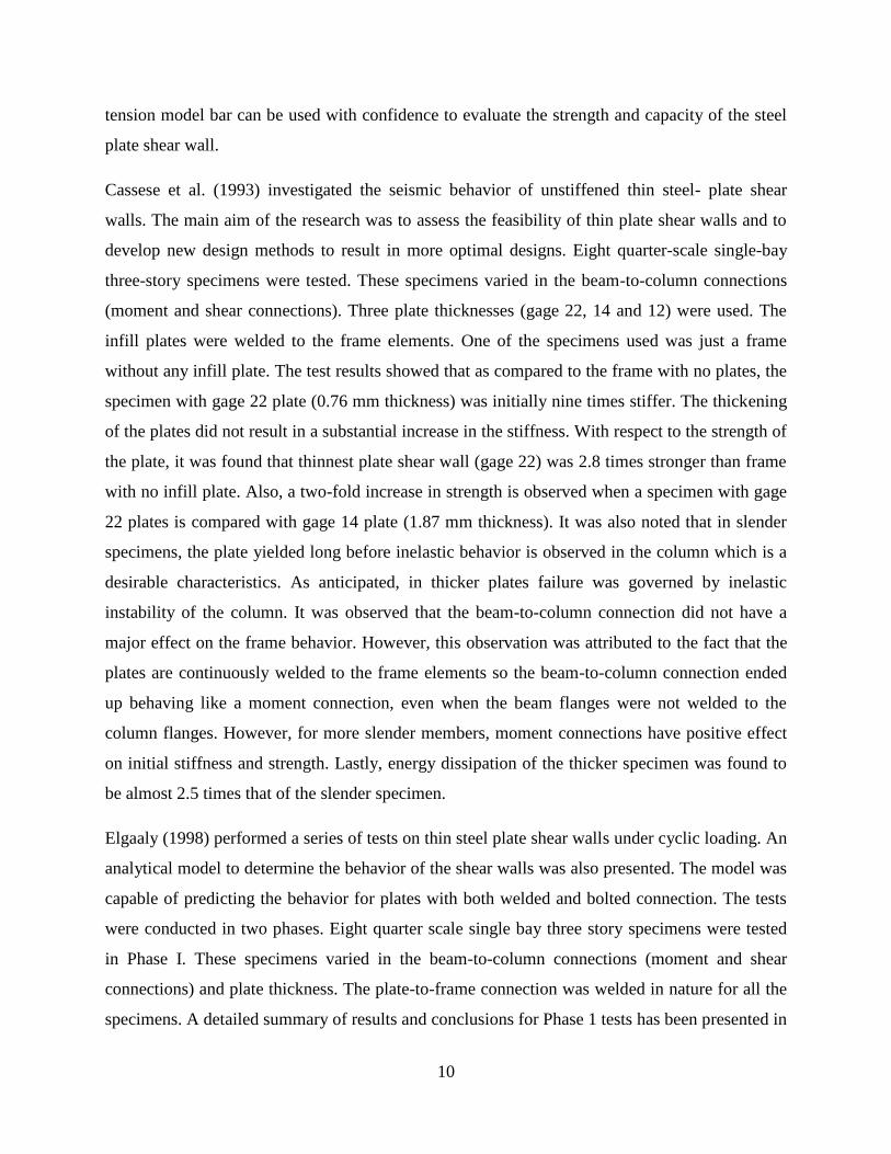
by the numerical models. Note that the strip model, shown in Figure 5, represents SPSWs as a

series of inclined strip elements, capable of transmitting tension forces only, and oriented in the

same direction as the average principal tensile stresses in the panel.

Figure 5: Diagrammatic representation of Strip Model [from (Lubell et al. 2000)]

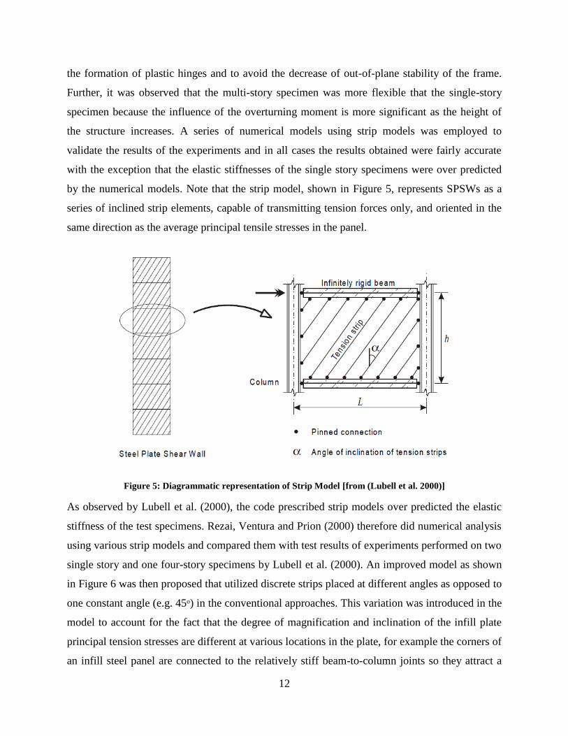
As observed by Lubell et al. (2000), the code prescribed strip models over predicted the elastic

stiffness of the test specimens. Rezai, Ventura and Prion (2000) therefore did numerical analysis

using various strip models and compared them with test results of experiments performed on two

single story and one four-story specimens by Lubell et al. (2000). An improved model as shown

in Figure 6 was then proposed that utilized discrete strips placed at different angles as opposed to

one constant angle (e.g. 45ᵒ) in the conventional approaches. This variation was introduced in the

model to account for the fact that the degree of magnification and inclination of the infill plate

principal tension stresses are different at various locations in the plate, for example the corners of

an infill steel panel are connected to the relatively stiff beam-to-column joints so they attract a

13

considerable portion of the steel plate membrane forces. This multi-angle strip model along with

three parallel strip models inclined at 37ᵒ, 45ᵒ and 55ᵒ respectively, was employed to numerically

analyze the specimens. After a thorough comparison of the analysis results with the experimental

results, it was concluded that the multi-angle strip model gave fairly accurate results for single-

story specimens and the first story of the four-story specimen. However, it was noticed that none

of the models could accurately predict the stiffness and strength of the fourth story. This was

attributed to the fact that due to the small overall aspect ratio of the four-story specimen there

was an increase in moment to base shear ratio, which resulted in a dominance of flexural

deformation compared to shear behavior. This effect can be significant for shear walls with

relatively light perimeter framing members which was the case for the specimens tested. It was

thus recommended that an improvement be made in the modeling technique to better capture the

behavior of multi-story structure at higher stories.

Figure 6: Diagrammatic representation of multi-angle strip model [from (Lubell et al. 2000)]

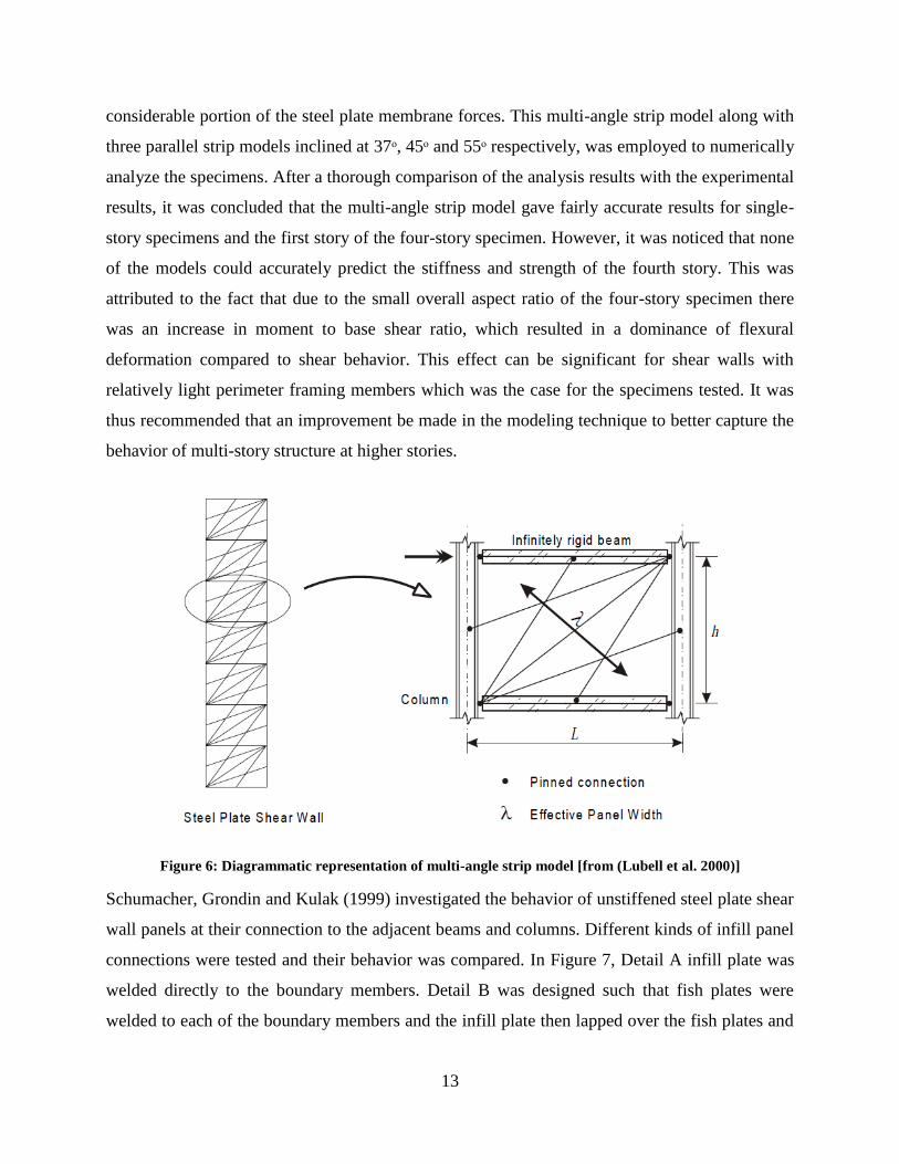
Schumacher, Grondin and Kulak (1999) investigated the behavior of unstiffened steel plate shear

wall panels at their connection to the adjacent beams and columns. Different kinds of infill panel

connections were tested and their behavior was compared. In Figure 7, Detail A infill plate was

welded directly to the boundary members. Detail B was designed such that fish plates were

welded to each of the boundary members and the infill plate then lapped over the fish plates and

14

welded. Finally, in Detail C, fish plate was welded to only one boundary member and then the

infill plate was welded directly to the other boundary member and lapped and welded onto the

fish plate. A fourth detail was a modified version of Detail B where two fish plates with a corner

cut-out were welded to the boundary members and the infill plate was then lapped

asymmetrically over the fish plates and welded. The cutout was made to reduce stress at corners.

The four details tested are shown in Figure 7. The loading strategy was adopted from ATC-24

(Applied Technology Council 1992) for experiments using quasi-static cyclic loading. Test

results concluded that each of the four infill connection performed satisfactorily under the quasi-

static loading. Cyclic inelastic response and energy dissipation capacity of all specimens was

comparable. It was also observed that the infill plate connection detail welded directly to the

boundary members was less susceptible to tearing than were the details that used fish plates.

However, due to the impracticality of such connections it cannot be used widely. It was found

that although modified Detail B connection delayed significant tearing of the corner detail, it did

not substantially improve the load-deformation behavior of the panel.

Figure 7: Infill panel connection details tested [from (Schumacher, Grondin and Kulak 1999)]

Berman, Celik and Bruneau (2005) performed cyclic testing on six frames. The main aim of their

experiments was to compare hysteretic behavior of light gauge steel plate shear walls and braced

15

frames. The aim was to design shear walls/ bracing systems that were strong enough to resist

necessary lateral forces and yet light enough to keep the existing structural elements from further

reinforcement. The flat infill plate (FP) was ASTM A1008 and had a thickness of 1.0 mm and

the boundary frame aspect ratio was 2.0. Continuous welded connection was used to connect the

infill plate to the boundary frame. Quasi-static testing was performed on the specimen in

accordance with the ATC-24 testing protocol. Specimen FP exhibited linear behavior during the

first six cycles of the testing. Buckling of the specimen started at 0.29% drift. The specimen was

successfully tested up to a drift of 3.7%, after which the testing had to be stopped due to

extensive damage to the plate. Overall, behavior of the specimen was ductile and stable up to

large drift levels, although pinching is also apparent from the hysteresis. Further analysis showed

that 90% of the initial stiffness of the system was due to the infill plate. Almost 50% of the

energy dissipated by the system was due to the infill plate. Also, the entire plate contributed to

the energy dissipation process. Another specimen on which the test was performed was a

corrugated infill plate specimen. The test setup and the load-deformation behavior of the SPSW

are shown in Figure 8.

a. Test Setup(from Berman and Bruneau 2005)

b. Load Deformation Behavior of SPSW (from Berman and Bruneau 2005)

Figure 8: Test conducted by Berman and Bruneau (2005) demonstrating SPSW behavior

The research work done on solid steel panels with normal strength steel can thus be broadly

categorized into two groups. The first group includes the work done by Thorburn, et al. (1983),

Elgaaly (1998), Rezai et al.(2000) and others in developing the analytical and numerical models

(e.g. the tensile bar model, multi angle strip model and other variations to the conventional strip

models) to predict the behavior of steel shear walls under various loading protocols and

boundary conditions. The second group includes the work done by Timler and Kulak (1983),

16

Tromposch and Kulak (1987), Berman et al. (2005), Cassese et al. (1993) and Lubell et al.

(2000) in verifying the proposed models and putting forward recommendations for better design

of steel plate shear walls through extensive experimentation. The major conclusions that can be

drawn from all the experiments performed on the steel plates walls are briefly summarized in the

following paragraphs.

Steel plate shear walls perform better than moment frames with no panels. As compared to the

moment frame with no plates, the specimen with 22 gage plate was initially nine times stiffer and

2.8 times stronger (Cassese et al.1993). The infill panels also performed better than most of the

singly braced frames as is clear from the experiments performed by Berman et al. (2005). The

infill plates could achieve a maximum drift of up to 3.7% in cases where the boundary members

or connections did not fail prior to the failure of the plates. Almost all the experiments performed

exhibited ductile and stable hysteresis behavior up to large drift levels. Experiments conducted

by Berman et al. (2005) concluded that almost 90% of the initial stiffness of the system was due

to the infill plate and about half of the total energy dissipation of the system was due to the infill

plate. It was also concluded that almost the entire plate contributed in dissipating energy, which

was another desirable characteristic of this system. Further, it was observed from the

experiments done by Tromposch and Kulak (1987) that these infill plate systems could achieve a

displacement ductility up to 6.8 which was later reaffirmed by the research done by Berman et al.

(2005), wherein he could achieve a displacement ductility of 12.

Although, the use of solid steel panels in the structural frames has advantages as compared to

bracing systems, the system also had a few shortcomings and the researchers faced some

challenges in implementing the concept. One of the major challenges faced was the failure of the

boundary members and the bolt/weld connections before the plates could reach their full

capacity. It is clear that the boundary members should elastically resist the moments associated

with plate tension and thus, it has been recommended that the boundary members be able to

resist the yield capacity of the plate acting at the inclined tension field angle. Experiments

performed by Tromposch et al. (1987) and Berman et al. (2005) brought out the fact that the

plates start to buckle at very low drifts of almost 0.29% which results in significant loss of

stiffness and leads to pinching of hysteresis curve. Also, it was observed in the experiments

performed by Berman et al. (2005) that buckling base shear for singly braced and X-braced

17

frames is higher under similar conditions. Also, post-buckling stiffness for plate walls is

considerably less than braced frames. Also, as the thickness of the steel plates decrease, it

becomes difficult to connect it to the boundary elements (Eatherton 2006).

2.1.2. Solid panel with Low Yield Strength (LYS) steel

Bruneau and Bhagwagar (2002) conducted non-linear analyses to investigate how structural

behavior is affected when thin infills of steel are used to seismically retrofit steel frames located

in regions of low and high seismicity. A typical three-bay frame extracted from an actual 20-

story hospital building in New York City was considered for this purpose. For loading purpose,

synthetic seismic ground excitation time histories were generated. Fully rigid and perfectly

flexible frame connection rigidities were considered to capture the extremes of frame behavior. It

was concluded from the study that the use of steel or any other ductile material as infill panels

can significantly reduce story drifts by as much as 200%. Also, this reduction in story drift can

be achieved without any significant increase in floor accelerations. It was also concluded that the

low yield strength steel infills behave slightly better (higher ductility ratio and lower story drifts)

than standard constructional grade steel under extreme seismic conditions but at the cost of some

extra material. It was noted that frames with LYS100 infills reached a maximum ductility ratio of

six which is about three times the ductility exhibited by frames having ordinary steel infills for

almost the same story drifts. They also exhibited lower fundamental vibration period. Further, it

was noted that steel plate shear walls may not be very effective in frames with aspect ratio

greater than three.

Vian and Bruneau (2005) investigated a set of three specimens: a solid steel infill panel (S2),

panel with twenty 200-mm-diameter (7.9 in.) holes (P) and a panel with quarter circle cut-outs at

the top corners (CR). LYS steel infill panels with reduced beam section (RBS) beam-to-column

connections at the top and bottom HBE was used. RBS was introduced in the beam design to

ensure sufficient ductility in the moment connections. It was observed that RBS reduced the end

plastic moment to 60.2% of the span plastic moment. A frame with an aspect ratio of 2:1 was

used for experimentation and 7 mm thick fish plates were used to connect the steel panel to the

boundary members. The infill panel thickness was 2.6 mm. A stable S-shape hysteretic curve

was achieved for specimen S2. The elastic stiffness was found to be 130 kN/mm. Elastic

buckling of the specimen started early at a drift of 0.1%, followed by initiation of yielding at

18

0.2%. Buckling folds were observed to be at an angle of about 27-35ᵒ. Finally, the test had to be

discontinued at a drift of 3%. The end of the test was marked by cracks in the bottom beam

flange at RBS, severe twisting of the columns, tension yielding of the panels with cracks in the

corner. Maximum base shear strength was found to be 2115 kN and high displacement ductility

of 10 was achieved. Finally, finite element analysis was done using ABAQUS to analyze the

specimens. Good agreement in the overall behavior was seen between the test results and the

FEM analysis.

Chen and Jhang (2011) investigated the behavior of low yield point (LYP) steel web plates in

single and multi-story frames. Four specimens with the width-to-thickness ratio varying from 50

to 150 were selected for the single-story frame test. Plate-type stiffeners were provided in the

first two specimens only. All the specimens in this test reached drift angles of about 4-5%

without significant decay in their strengths. The buckling started at a drift of about 2-3% for

specimens with b/t ratio less than or equal to 80, whereas for specimen with b/t larger than 80, it

started as early as 1% drift. Therefore to delay the onset of buckling, a b/t ratio less than 80 is

desirable. The maximum shear buckling strength was observed in the specimen with a b/t ratio of

80 and with no stiffeners. It was argued that the boundary elements provided much stronger

restraints as compared to conventional plate-type stiffeners. It was concluded that relatively low

b/t ratio result in higher buckling strength.

The experimental data was compared to the theoretical values obtained from inelastic buckling

stress equation given by Galambos (1987). The difference between the experimental and the

theoretical data was found to be less that 14%. For the multi-story frame test, two steel panel

specimens were chosen. Beam-to-column connection was a rigid moment type for the first

specimen, while for the second specimen, a simple shear type connection was adopted. Both of

the specimens displayed stable hysteretic behavior up to a large drift of 5% and significant

inelastic tension field was developed at their ultimate strength. It was observed that the frame

with moment connections displayed higher stiffness than the one with shear connection. This

difference exceeds 30% after the onset of yielding, but gradually reduces at higher drifts. Also, it

was noted that moment connections enhanced the strength and energy dissipation capacity of the

frame by 28% and 18% respectively. Both the specimens reached a maximum drift of about 6%.

It was concluded that the pinching behavior that is usually observed in conventional thin steel

19

shear walls under in-plane load, could be alleviated due to the use of LYP web plates. The LYP

steel also has superior elongation capacity and display significant strain-hardening in the post

yield stage.

2.2. PANEL WITH CORRUGATED PLATES

Berman and Bruneau (2005) conducted experiments to study the hysteretic behavior of braced

frames and frames with steel infill plates. As mentioned previously, one of these specimens

consisted of a corrugated infill plate (cold formed steel deck). The corrugations were inclined at

45ᵒ from the horizontal. This was done to force the inclination angle of the tension field to be

45◦. The corrugated plate was sandwiched between two angles that were bolted to the boundary

frame. The plate was connected to the angles through epoxy. The infill plate consisting of four

pieces was fastened together using 1.6 mm diameter steel pop-rivets. The hysteretic behavior

was elastic in the first three cycles. Buckling started at about 0.44% drift. The failure of pop-

rivets and cracking in epoxy was observed at about yield displacement. The specimen was

successfully tested to a maximum displacement of 40.6 mm (2.2% drift). Failure of the specimen

was from fractures of the infill plate at locations of repeated local buckling. As anticipated, the

hysteresis of the specimen was one-sided because the tension-field action only took place when

the corrugations were in tension. The infill contributed to about 90% of the initial stiffness of the

system. A displacement ductility of 3 was achieved. It was observed that more than 67% of the

total energy dissipated was due to the infill plate. However, total energy dissipated was less than

one-fifth of that achieved by solid steel panel.

Stojadinovic and Tipping (2008) proposed a shear wall system that utilized a low profile metal

deck as sheathing which was fastened to light-framed cold-formed steel framing with screws.

The term “corrugated sheet steel shear wall” or CSSSW was used to describe thissystem. The

main purpose of this research was to provide the practicing engineers with a stronger, stiffer and

less expensive lateral bracing system. Cyclic loading tests were performed on 44 specimens. The

six design variables that were varied during the test were: gauge of the corrugated sheet steel (22

gauge, 20 gauge and 18 gauge), gauge of the studs and tracks, fastener type/size, fastener spacing

for attachment of corrugated sheet steel, inclusion of gypsum board on one side and application

of the corrugated sheet steel on one or both sides of a wall specimen. For connections, note that

the sheathing (corrugated plates) was fastened to the stud and the stud in turn was fastened to the

20

boundary elements. To facilitate installation and removal of the specimens from the test frame,

attachment plates were fastened to the perimeter of the specimens with self-drilling sheet metal

screws. These plates, in turn, were fastened to the test frame with High Strength bolts. Test

results showed that in all the cases the failure mode of the specimen was the popping out of the

screws due to warping of the corrugated plates. In all cases, the first screws to pop out were

located in the boundary members. Further, the comparison of the results showed that using of

gypsum board had little effect on the strength and stiffness of the CSSSW. To determine the

effect of adding the corrugated sheet steel to both sides of a specimen, two specimens were

tested. It was concluded that double sided walls can achieve double the shear strength.

2.3. PERFORATED STEEL PLATE SHEAR WALLS

Perforated steel plate shear walls such as shown in Figure 9, are shear walls with single or

multiple circular holes. These shear walls were developed by the researchers to allow for utility

access. These perforations also served as a method of reducing the panel strength and in turn the

demand on the reducing frame. This characteristic was believed to be beneficial in markets that

do not have low yield strength (LYS) steel readily available.

Figure 9: Perforated steel plate shear walls [from (Roberts et al. 1992 and Vian et al. 2005)]

21

Roberts and Sabouri-Ghomi (1992) performed a series of sixteen quasi-static cyclic loading tests

on unstiffened steel shear walls with centrally placed circular openings of varying diameters.

Panels with aspect b/d ratio of 1 and 1.5, thicknesses of 0.83mm and 1.23 mm and circular

opening diameter ranging from 0 to 150 mm were used. The plates were clamped between rigid

pin-joined frame elements. Experiment results demonstrated that all the panels tested exhibited

stable hysteresis loops. All the panels exhibited adequate ductility for the first four loading

cycles without significant loss in the load-carrying capacity. It was observed that the stiffness

and the ultimate strength of the panels reduced linearly with the increase in the diameter of the

circular openings. Roberts and Sabouri-Ghomi (1992), therefore suggested that the strength and

the stiffness of a perforated plated can be approximated conservatively by applying a reduction

factor of (1-D/d) (where, D is the perforation diameter and d is the height of the panel) to the

strength and the stiffness of a similar un-perforated plate. In another paper, Roberts and Sabouri-

Ghomi (1991) developed an analytical model to predict the hysteretic behavior of the unstiffened

steel shear walls. This model was modified using the reduction factor and the results were

compared with the experimental data. Using a reduction factor of (1-D/d) implied completely

neglecting the contribution of steel of width equal to the diameter of the opening along the

diagonal. Therefore, as anticipated it was found that the model gave conservative values. Other

factors which lead to conservative results were that strain hardening was neglected and the plate

boundaries were treated as simply supported, thus underestimating the critical load.

Vian and Bruneau (2005) conducted experiments to investigate the efficiency of steel infill

panels with circular openings. They came up with an effective reduction factor to account for

reduced stiffness and strength of panels with multiple circular holes. The test set-up and the

specimen (specimen CR) dimensions were identical to those mentioned in the previous section.

After considering a number of options for the hole diameter and spacings, the final design of the

infill panel had 20 circular openings staggered to be aligned diagonally at 45ᵒ, with a diameter of

200 mm and horizontal/vertical spacing of 300 mm. This pattern of circular openings would

reduce the stiffness of the panel by 17% as predicted by the reduction factors developed by Vian

et al.(2005) The specimen displayed stable S-shaped hysteresis loops with little pinching.

Observed elastic stiffness was 115 kN/mm. Yielding was first observed at a drift of 0.3%. At

1.2% drift, the RBS connection started yielding at the top beam connection. At 2.5% drift,

yielding and buckling of the fish plate was observed in addition to the web local buckling at the

22

bottom beam RBS connection. The test was finally stopped at 3% drift when a column continuity

plate fractured. Although the web panel had not fractured at this drift, severe damage and

distortions to the panel had made it impractical to continue testing. The elastic strength and

elastic stiffness of the specimen were found to be 85.5% and 81.5% respectively, as compared to

a solid panel of same dimensions. This was in good agreement with the value predicted earlier.

The maximum base shear achieved was 1790 kN. A displacement ductility of 10 was achieved

when the test stopped.

Moghimi and Driver (2011) investigated the influence of perforations on steel plate shear walls

by comparing them with similar SPSW systems with no perforations in their infill plates. For the

purpose of this study, a set of three four-story walls were chosen. Set A consisted of solid walls

whereas set B and C consisted of walls with circular opening. They had 18 openings each on the

top-most story. For the other three stories, set B had 22 openings as opposed to set C which had

23 openings. All the openings were regularly spaced vertically and horizontally (at a distance of

280 mm) over the entire area of the infill plates. Note that each set consisted of two specimens

which were identical to each other, but employed different beam-to-column connection- moment

and shear connections. According to the perforation patterns, it was predicted that the shear

resistance of the perforated wall should be 0.6 times that of a solid wall. The pushover analysis

showed that a reduction factor of 0.6 was a conservative evaluation. The most notable finding of

the paper was associated with the force demand of the shear walls. It was found that, although

the perforations reduce the shear capacity of the infill plate considerably, they may not reduce

the force demands on the columns, especially at the upper stories where the perforations make

the design strength ratios worse. These results are in contrast the main idea behind the

development of this system and also highlight an inherent uncertainty in the response of the

perforated plates.

2.4. PANEL WITH QUARTER-CIRCLE CUTOUTS

As a continuation of the experiments performed by Vian and Bruneau (2005) on LYS steel

panels, tests were done on a specimen with quarter-circle cutouts at the four corners of the web

plate. The main purpose of the cutouts was to provide access to utilities. Also, the corner cutouts

are a favorable feature because they provide more flexibility to accommodate angle change at the

frame corners during sway. This results in lower end moments along the length of the arc. An arc

23

section 160mm wide and 19mm thick was chosen after preliminary calculations. The other plate

dimensions were identical to the ones mentioned in Section 2.1.2.The hysteresis curve obtained

was stable with little pinching. As observed in other specimens tested by Vian and Bruneau,

buckling of the panel started at a drift of 0.1% and yielding initiated at 0.3% drift. The fish plate

started buckling at 1.5% drift. At about 3% drift fractures of the beam RBS was observed in

addition to the fractures in the infill plates. At about 4% drift, a loud bang was heard, followed

by a reduction in the strength of about 24-35% in the subsequent cycle of the same amplitude. At

this drift, the test had to be stopped due to safety issues. The infill plate could have resisted

loading to larger deflections, but the testing had to be concluded to prevent lateral support

damage. The end of the test was marked by local buckling of the fish plates, severe tears in the

panel interior, weld tears in the top bam top flange continuity plates and twisting of the columns.

The maximum base shear strength was noted as 2050 kN which was quite comparable to that of

an identical panel with no cutouts. An elastic stiffness of 140kN/mm and a displacement ductility

of 13.33 were achieved by the specimen.

2.5. SLIT STEEL PLATE SHEAR WALLS AND RELATED SHEAR FUSE

PLATES

2.5.1. Panel with rectangular slits

Panels with rectangular slits such as shown in are steel shear walls with vertical slits equally

spaced, forming columns of links. When subjected to lateral loading, these links behave as

beams in double curvature, dissipating energy in flexural. Numerous variations in these types of

panels have been investigated in the past.

24

Figure 10: Steel plate walls with rectangular slits [from (Hitaka et al. 2006)]

Hitaka, Matsui, Tsuda and Sadakane (2000) conducted experiments on slit panel shear walls with

beam-to-column rigidity ratio and the strength/stiffness of the shear wall as the test parameters.

The main aim of the test was to bring out the mutual effects of the wall and the frame when

attached to each other. Three sets of frames were used: one with beam-column rigidity ratio

larger than 1 and the other, less than 1. In the other set of frames two kinds of shear walls; one

stronger and stiffer than the other. Last set of two frames did not have any shear wall. Stiffeners

were welded at both sides of the wall to prevent out-of-plane deformation. All the specimens

showed stable hysteresis with little or no pinching. A maximum drift of more than 4% was

observed in all the specimens. As compared to the frames with infinite stiffness, the behavior of

these specimens was relatively unstable. It was noted that the wall contributes greatly to increase

the stiffness of the structure. Also, there is a modest increase in the frame stiffness with the

addition of shear wall. It was also noted that for the same story drift, the vertical force transferred

from beam to the shear wall is smaller in the case where the beams are not infinitely rigid. With

respect to energy absorption capacity, it was observed that the shear wall contributed to almost

70-80% of the total energy absorption capacity of the system.

Hitaka and Matsui (2003) introduced the steel plate shear walls with vertical slits. In this system,

the segments between the slits formed a series of flexural link and provided a fairly ductile

response. Hitaka and Matsui came up with equations to predict the initial stiffness and the

25

ultimate strength of the slit panels. Also, a series of four tests (A, B, C, D) were conducted on a

total of 42 specimens. Test series A and B focused on the behavior of shear walls with varied slit

parameters (b/t, L/t, number of slits in a row, number of rows). The objective of the Series C was

to study the transverse behavior of the slit walls with and without transverse stiffening. Series D

tests examined the shear wall behavior under different loading protocols. Steel panels for all

specimens had the dimensions of 800 mm by 800 mm by 34.5 mm, which is about one-quarter to

one-third of the full scale applications. All the specimens other than the Series C specimens were

stiffener stiffened.

Except for a few, all specimens underwent story drift of more than 3% without initiation of

cracks or abrupt strength degradation. The response was pretty linear until the force reached one-

third of its maximum, after which the response softened until reaching the maximum strength. At

about 5% drift, all the specimens experienced transverse deformation which resulted in post-peak

strength degradation. In general, this post peak strength degradation was stable for almost all the

elements. At about 2% drift some specimens saw initiation of cracks at slit ends. These cracks

propagated further and led to the ductile fractures in some specimens at 4% drift which in turn

resulted in substantial strength degradation. It was however concluded that the main cause of

strength degradation was transverse buckling of the plate, rather than the ductile fractures.

With respect to the parametric design, b/t ratio of the flexural link was found to be most

influential parameter. A major observation to back up this idea was that all the specimens with

b/t ratio of 10 did not display any transverse deformation up to a drift of 2.5%, whereas all the

other specimens this deformation took place before a drift of 2%. By comparing specimens with

equal plastic strength, it was noted that specimens with higher β ratio (ratio of total link length to

the wall height) displayed higher ultimate strength. Regarding the out-of plane deformations, a

few major conclusions could be drawn. Firstly, Stiffening enhances the maximum strength of a

specimen and the drift at which it experiences an increase in out-of-plane deformation. In

stiffener-stiffened specimens, it was observed that specimens with relatively large b/t and L/b

ratios suffered pinching when inner links deformed out of plane. Contrary to this, specimens with

relatively large b/t ratios and smaller L/b ratios, experienced out-of plane deformation of the

entire panel. This behavior was similar to panels buckling in shear which eventually led to

pinching of the hysteresis curves. It was also noted that controlling the b/t, L/t and L/b ratios can

26

help restraining the links from flexural torsional buckling. The aspect ratios of the links were

thus concluded to be of paramount importance in the behavior of the panels.

Cortes and Liu (2008) discuss the behavior of steel slit panels (SSP) as an independent unit and

as a part of lateral force resisting system (LFRS) and put forward the idea of three different SSPs

that may be used for the system. The SSPs discussed here differ from the panels tested by Hitaka

and Matsui (2000, 2003) in that the aspect ratio of the panel is 1:2 instead of 1:1. Also, the main

objective of the design of SSPs was to resist the entire base shear in the SSP instead of just a

fraction. In general, the behavior of panels tested by Hitaka and Matsui was similar to SSPs, but

the global behavior of a frame with SSP is quite different. Cortes and Liu have suggested the

consideration of gravity loads while analyzing the SSP designs. Panel strength and frame

stiffness have been pointed out as important factors that influence behavior of LFRS. A flexible

beam will result in the reduced stiffness of a Steel Slit Panel Frame (SSPF). Also, the stiffness

provided by a panel also depends on the story in which it is located. It has also been noted that

the stiffness of the SSP depends on the shear stiffness of the zones above, below, and between

links and the shear and flexural stiffness of the links. Finally, three designs for SSPs have been

presented (Panel T1, T2 and BR). The first panel (T1) had three rows of nine links. It is simple to

fabricate and dissipates great amount of energy. Panel T2 had two rows of eight links and was

stiffer than T1. T2 employs stiff stub beams at the top and bottom of the panel which is capable

of increasing the overall stiffness. Finally, Panel BR had the same dimensions as Panel T1,

however a brace was provided over the links to reduce their buckling. Panel T1 and BR had

bolted connections to the loading frame in addition to the edge stiffeners to provide extra

stiffening. The experimental results for this panel have been discussed in the next section.

Tests were performed on panel T1 with two different thicknesses. The hysteresis curves obtained

from both the tests were flat and stable up to large drifts. The test results showed that both the

specimens first yielded at 0.125% drift. Although both specimens suffered lateral torsional

buckling, for the thicker T1 panel this type of buckling was observed at 4% drift, as opposed to

its counterpart, where it was observed at 2% drift. Both the specimens experienced failure of

flexural links at the end of 7% drift, which led to the conclusion of the test. The thicker panel

could resist a maximum load of 28.8 kips as opposed to the thinner plate which could only resist

a maximum load of 19.8 kips. As anticipated the thicker plate had a higher initial stiffness of

27

72.6 k/in as compared to the thin panel which had stiffness of 50.6 k/in. Another test was

performed on Panel type T2, with a panel thickness of 3/16’’. This panel exhibited shear

buckling a tension field action at a drift of about 2%. Two main factors that are believed to have

caused the tension field action and the shear buckling are the boundary conditions and the aspect

ratio of the panel. This panel was welded to the stub beams along its entire width. This created

more rigid boundary conditions as compared to the other specimens which had bolted

connections. For the panels with bolted connections, the distance from the edge stiffener to the

first bolt was not restrained, allowing some rotation to take place. This small rotation proved

beneficial in preventing the tension diagonals or shear buckling from occurring. In addition, the

width to height aspect ratio of this panel was approximately 0.6. This panel was relatively wider

than all other panels which had an aspect ratio of approximately 0.4.

These conditions, found exclusively in this panel, were the main cause for the generation of the

apparent tension field action and shear buckling of the panel. Apart from this, lateral torsional

buckling of the panel was also observed at a drift of 1.5%. The test had to be concluded early at

5% drift due to fracture in the links. The specimen however has a comparable maximum strength

of 24.4 kips and a high stiffness of 80 k/in. the main problem with Panel T2 was the difficulty in

installation. The height of the panel was detailed to be the same height as the frame, thus very

little space, if any, was available. It was therefore recommended that if this panel was to be

specified for use in a building, it would be necessary to leave some space for constructability

purposes.

Cortes and Liu (2009) discussed the advantage of steel slit panels as lateral force resisting

system. Their work focused on the design aspect of the slit panels. The main parameters to be

considered when designing a steel slit panel (SSP) are: α (length to width ratio of the link), β

(fraction of panel height that is composed of the links) and the links cross-section aspect ratio b/t.

The b/t ratio is important as it influences the buckling of the links and should be ideally between

10 and 15. The geometry of the panel was chosen according to the load demand. The number of

panels on each story was decided according to the strength of each story. Once the geometry and

the number of panels were decided, the stiffness and the strength of the panel were obtained as

the sum of shear forces acting on the links when they reach the plastic moment. The designer

must also ensure that global lateral-torsional buckling of the panels do not occur at an early

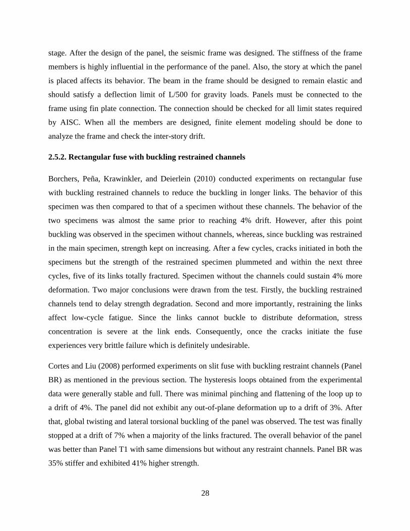
28

stage. After the design of the panel, the seismic frame was designed. The stiffness of the frame

members is highly influential in the performance of the panel. Also, the story at which the panel

is placed affects its behavior. The beam in the frame should be designed to remain elastic and

should satisfy a deflection limit of L/500 for gravity loads. Panels must be connected to the

frame using fin plate connection. The connection should be checked for all limit states required

by AISC. When all the members are designed, finite element modeling should be done to

analyze the frame and check the inter-story drift.

2.5.2. Rectangular fuse with buckling restrained channels

Borchers, Peña, Krawinkler, and Deierlein (2010) conducted experiments on rectangular fuse

with buckling restrained channels to reduce the buckling in longer links. The behavior of this

specimen was then compared to that of a specimen without these channels. The behavior of the

two specimens was almost the same prior to reaching 4% drift. However, after this point

buckling was observed in the specimen without channels, whereas, since buckling was restrained

in the main specimen, strength kept on increasing. After a few cycles, cracks initiated in both the

specimens but the strength of the restrained specimen plummeted and within the next three

cycles, five of its links totally fractured. Specimen without the channels could sustain 4% more

deformation. Two major conclusions were drawn from the test. Firstly, the buckling restrained

channels tend to delay strength degradation. Second and more importantly, restraining the links

affect low-cycle fatigue. Since the links cannot buckle to distribute deformation, stress

concentration is severe at the link ends. Consequently, once the cracks initiate the fuse

experiences very brittle failure which is definitely undesirable.

Cortes and Liu (2008) performed experiments on slit fuse with buckling restraint channels (Panel

BR) as mentioned in the previous section. The hysteresis loops obtained from the experimental

data were generally stable and full. There was minimal pinching and flattening of the loop up to

a drift of 4%. The panel did not exhibit any out-of-plane deformation up to a drift of 3%. After

that, global twisting and lateral torsional buckling of the panel was observed. The test was finally

stopped at a drift of 7% when a majority of the links fractured. The overall behavior of the panel

was better than Panel T1 with same dimensions but without any restraint channels. Panel BR was

35% stiffer and exhibited 41% higher strength.

29

2.6. BUTTERFLYFUSE

2.6.1. Panels with butterfly fuse

The experiments conducted by Borchers, Peña, Krawinkler, and Deierlein (2010) at Stanford

University were focused on the behavior of slit fuse and butterfly fuse panels. Figure 11 shows

one on the butterfly fuse panels tested. The major of the test specimens were the L, b, t, b/t, L/t,

ws (diameter of the rounded slit ends) and a/b ratio in case of butterfly fuse. A total of six

specimens were tested.

The test results showed that unlike the rectangular slit fuse panels where the yielding initiated at

the slit edge, butterfly fuse panels had yielding concentrated at around the quarter height of the

panel. As the deformation increased, it got distributed along the edge of the slit indicating a

proper distribution of yielding. Near the end, buckling became so severe that the links turned 90

degrees and became perpendicular to the loading direction. However, it was observed that

butterfly fuse could sustain more deformation and was able to withstand higher load at large

drifts.

Two main reasons were brought up for this kind of behavior. First, the uniform yielding along

the edge of the link in the butterfly fuse reduced strain concentration at a particular point on the

link and thus, delayed crack initiation. Second, since the plastic hinge formation took place at

quarter height sections in the butterfly link, the effective length of the link in tension was shorter

as compared to the links in slit fuse where the hinges are formed at the slit ends. Due to shorter

length of the tension portion, it could contribute more to the lateral strength. Another butterfly

fuse which had a relatively larger L/t ratio was tested. It was found that buckling in this specimen

was delayed. This differences was however not very significant and it was be concluded that L/t

ratio is not very influential in butterfly-fuse performance. Test results of a specimen with a very

small b/t ratio (=6) showed that thick fuses can sustain stable hysteretic behavior up to much

larger drifts. Buckling was also delayed. This in turn increased the total energy dissipation. The

ultimate deformation however was similar. It was thus concluded that a smaller b/t ratio

improved stability and energy dissipation. Another specimen with a still smaller b/t ratio (=2)

was tested. It was found that very thick butterfly fuse exhibited stable hysteresis behavior

throughout the test. Due to strain hardening, the ultimate strength exceeded twice the design

30

strength. The main findings of this test was that when the fuse is thick enough, buckling can be

prevented which implies more energy dissipation. However, their over-strength due to strain

hardening might be an undesirable after-effect. Overall, all the butterfly fuses acted in a more

ductile manner as compared to the slit fuse panel.

Figure 11: Panel with butterfly fuse [from (Borchers, Peña, Krawinkler, and Deierlein 2010)]

2.6.2. Panels with butterfly fuse attached to a backing plate

Borchers, Peña, Krawinkler, and Deierlein (2010) conducted experiments on butterfly panels

with backing plate connection. The results obtained from these specimens were then compared to

the ones where no backing plate was provided. It was found that they behaved the same up to a

drift of 2.4%. However, after buckling, there was more decrease in strength of the panel without

backing plate. After the formation of the tension field, the strength in the fuse with backing plate

is 5-10% higher due to the friction between the fuse and the backing plate. The fatigue behavior

was also quite different for both the fuses. B10-36W did not show any signs of cracks until a

drift of 20% as compared to a drift of 14% in the unrestrained fuse. This was because in the

unrestrained fuse, the links formed a hinge in the middle due to compression which incurred a lot

of repeated rotation in addition to tension deformation. These conditions led to the fracture of

this fuse at such locations. When a thick butterfly fuse (b/t=7) was used with backing plate

connection, the most important finding which came out was the damage to the fuse due to over-

strength as previously mentioned. At a drift of about 17%, the strength of the fuse exceeded 1.5

times the design strength. The weld was not designed to take up this kind of load and it failed

causing the strength to drop down drastically. It was therefore of extreme importance that the

connections in slit and butterfly fuses are designed to account for the over-strength due to a

31

combined effect of tension and strain-hardening. If adequately accounted for this idea, backing

plate is a viable connection detail.

2.7. DISSIPATIVE DEVICES EMPLOYING THE RING-LINK SYSTEM

R.G. Tyler (1985) described the tests on a dissipative device carried out by David Smith and

Robert Henry in Auckland, New Zealand in 1970s. This device, also known as yielding frames,

dissipate energy through the yielding of the round bars which constitute them. The yielding

frame shown in Figure 12 is geometrically similar to the framework in which it was

incorporated.

When subjected to lateral loading, this device deforms into a parallelogram and develops no

slack along the diagonals, as experienced by conventional cross-bracing systems when subjected

to racking deformations. The yielding frame thus exhibits stable cyclic behavior. Cyclic tests on

bracing systems incorporating the yielding frames showed that many hundreds of cycles can be

completed without the development of much slack in the braces. Thus, the proposed bracing

system was proved to be reliable in providing stable earthquake resistance.

Figure 12: Yielding frame with constant cross-section [from (Tyler 1985)]

Ciampi and Samuelli-Ferretti (1990) also proposed a class of dissipating devices based on

flexural yielding of steel. As mentioned above, these yielding frames are geometrically similar to

the main framework and connected to its joints through tension-only braces. Under lateral cyclic

32

loading, the yielding frame deforms inelastically while keeping both the connecting braces in

tension. This results in a fully dissipative hysteretic response.

Figure 13: Yielding frame with varying width [from (Ciampi and Samuelli-Ferretti 1990)]

Figure 14: Yielding frame with varying depth [from (Ciampi and Samuelli-Ferretti 1990)]

The energy yielding frame is cut out from a thick steel plate. Unlike the system presented by

Tyler (1985), the cross-section of the yielding frame has a tapered shape which is anti-symmetric

to the flexural moment distribution that develops in it during the lateral displacement of the

whole system. Two variations to this device were proposed-one with linearly variable width as

shown in Figure 13 and the other with linearly variable depth shown in Figure 14. This type of

varying cross-section ensures that the device experiences uniform distribution of plastic

deformation.

This device was tested separately as well as in the form of one-bay one-story frame system. In all

cases, the system was efficient and exhibited good dissipation capacity and long cyclic life.

However, these devices exhibited undesirable expansion as a result of excessive plastic

deformation. In real applications, this kind of expansion may have adverse effects on the

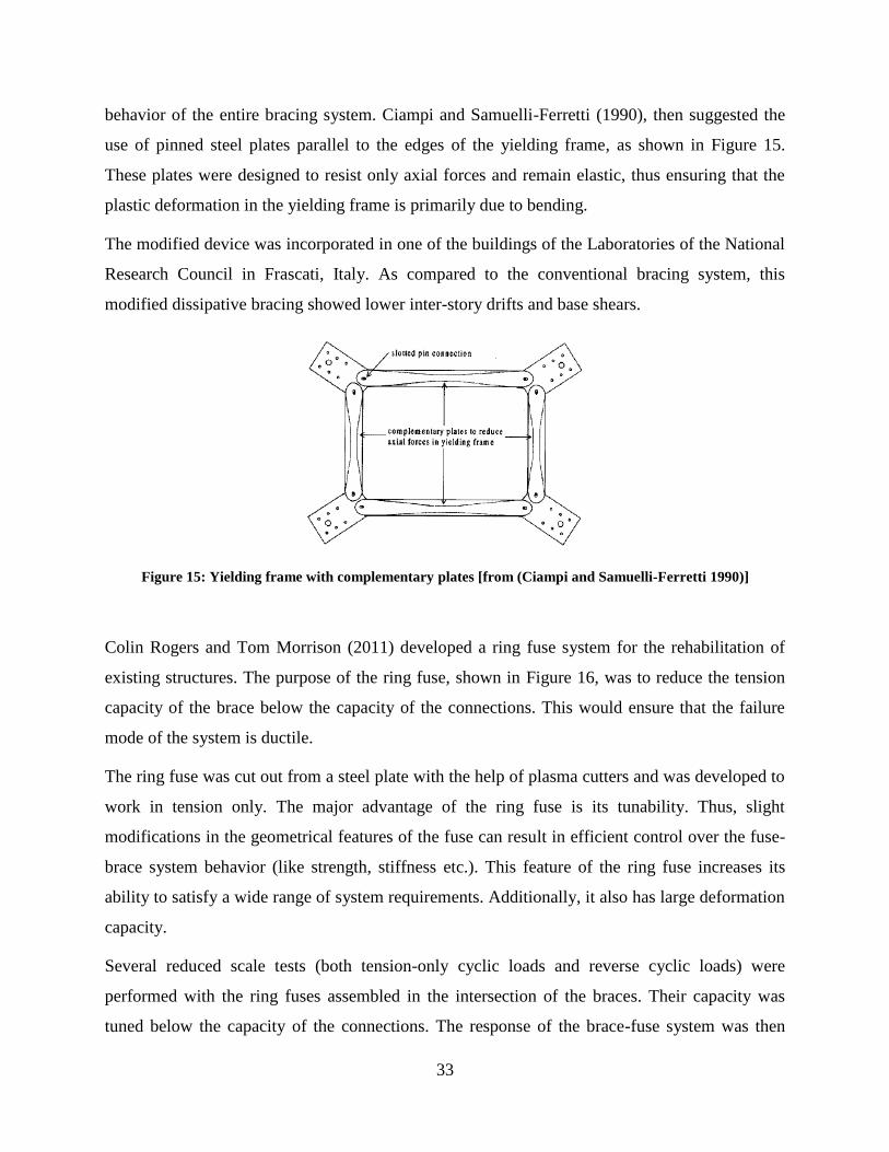
33

behavior of the entire bracing system. Ciampi and Samuelli-Ferretti (1990), then suggested the

use of pinned steel plates parallel to the edges of the yielding frame, as shown in Figure 15.

These plates were designed to resist only axial forces and remain elastic, thus ensuring that the

plastic deformation in the yielding frame is primarily due to bending.

The modified device was incorporated in one of the buildings of the Laboratories of the National

Research Council in Frascati, Italy. As compared to the conventional bracing system, this

modified dissipative bracing showed lower inter-story drifts and base shears.

Figure 15: Yielding frame with complementary plates [from (Ciampi and Samuelli-Ferretti 1990)]

Colin Rogers and Tom Morrison (2011) developed a ring fuse system for the rehabilitation of

existing structures. The purpose of the ring fuse, shown in Figure 16, was to reduce the tension

capacity of the brace below the capacity of the connections. This would ensure that the failure

mode of the system is ductile.

The ring fuse was cut out from a steel plate with the help of plasma cutters and was developed to

work in tension only. The major advantage of the ring fuse is its tunability. Thus, slight

modifications in the geometrical features of the fuse can result in efficient control over the fuse-

brace system behavior (like strength, stiffness etc.). This feature of the ring fuse increases its

ability to satisfy a wide range of system requirements. Additionally, it also has large deformation

capacity.

Several reduced scale tests (both tension-only cyclic loads and reverse cyclic loads) were

performed with the ring fuses assembled in the intersection of the braces. Their capacity was

tuned below the capacity of the connections. The response of the brace-fuse system was then

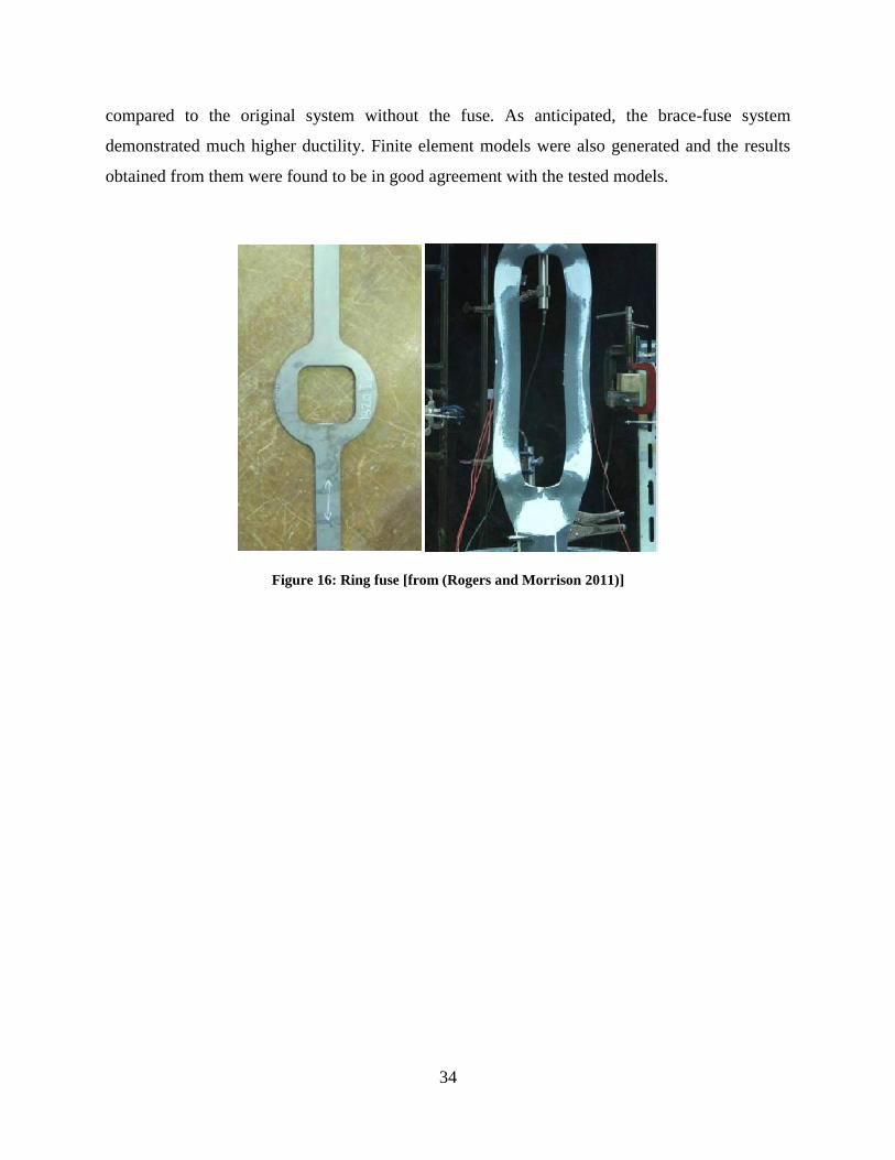
34

compared to the original system without the fuse. As anticipated, the brace-fuse system

demonstrated much higher ductility. Finite element models were also generated and the results

obtained from them were found to be in good agreement with the tested models.

Figure 16: Ring fuse [from (Rogers and Morrison 2011)]

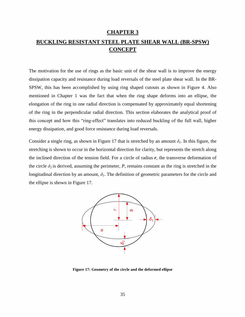
35

CHAPTER 3


CONCEPT

The motivation for the use of rings as the basic unit of the shear wall is to improve the energy

dissipation capacity and resistance during load reversals of the steel plate shear wall. In the BR-

SPSW, this has been accomplished by using ring shaped cutouts as shown in Figure 4. Also

mentioned in Chapter 1 was the fact that when the ring shape deforms into an ellipse, the

elongation of the ring in one radial direction is compensated by approximately equal shortening

of the ring in the perpendicular radial direction. This section elaborates the analytical proof of

this concept and how this “ring-effect” translates into reduced buckling of the full wall, higher

energy dissipation, and good force resistance during load reversals.

Consider a single ring, as shown in Figure 17 that is stretched by an amount δ1. In this figure, the

stretching is shown to occur in the horizontal direction for clarity, but represents the stretch along

the inclined direction of the tension field. For a circle of radius r, the transverse deformation of

the circle δ2 is derived, assuming the perimeter, P, remains constant as the ring is stretched in the

longitudinal direction by an amount, δ1. The definition of geometric parameters for the circle and

the ellipse is shown in Figure 17.

a

δ1

b

δ2

r

Figure 17: Geometry of the circle and the deformed ellipse

36

The approximate perimeter of an ellipse, Pellipse, is given by Equation 3.1, where a and b are the

major and minor radii of the ellipse, respectively as shown in Figure 12.

√

(3.1)

The perimeter of the circle, Pring, is given by Equation 3.2.

(3.2)

Equating the two perimeters results in Equation 3.3,

√

(3.3)

The values for a and b can be related to the radius and deformations as given in Equation 3.4

a = r+δ1andb = r-δ2 (3.4)

Substituting these values in the Equation 3.3 and squaring both the sides gives:

(3.5)

Expanding the terms and solving the quadratic equation for δ2results Equation 3.6.

2 2

2 1 1

14 4 8

2r r r

(3.6)

The variation in transverse deformation, δ2, resulting from longitudinal stretching, δ1, is shown in

Figure 18. The plot highlights several key points relevant to the BR-SPSW concept. The curve

labeled “Ring” in the plot shows that for small applied deformations, the longitudinal and

transverse deformations are nearly equal in magnitude. If the ratio of transverse deformation to

the longitudinal deformation (δ2/δ1) is thought of as an effective Poisson’s ratio of the ring unit,

the slope of the “Ring” curve would give the effective Poisson’s ratio. For small deformations

this ratio is nearly unity. In a steel plate shear wall, an effective Poisson’s ratio close to unity is

desirable because it implies that when a material is subjected to longitudinal stretching, the plate

would experience negligible slack in the transverse direction. To understand how this effect

translates into a full scale shear wall system, consider an idealized BR-SPSW model subjected to

37

a small story drift Δ, as shown in Figure 19. The rings along the tension diagonal will elongate

by a similar amount (L+Δ) as the compression diagonal is shortening (L-Δ), essentially pulling

the plate taught in the transverse direction, thus resisting the tendency for the plate to buckle.

δ2δ1

δ2

δ1

Ring

Solid Plate

Excess material

in transverse

direction causes

buckling

No slack in

the transverse

direction

δ1

δ2

a. Ring b. Solid Plate c. Relationship Between δ1 and δ2

Figure 18: Concept showing how the ring eliminates slack in the direction transverse to the tension diagonal

Com

pression

Diagon

al (L-Δ

)Tensio

n Dia

gonal (L+Δ)

δ

δ: Interstory Drift

L: Initial length of the diagonal

Figure 19: BR-SPSW subjected to lateral load

38

When compared to a standard SPSW wall, which exhibits an approximate Poisson’s ratio equal

to the Poisson’s ratio of the steel material used (generally 0.3), this is a great improvement

because an effective Poisson’s ratio of 0.3 would mean that shortening of the solid plate material

in the transverse direction is approximately 30% of the elongation in the longitudinal direction.

This results in a slack due to excess material in the transverse direction which causes the

buckling of the solid plate.

39

CHAPTER 4

VALIDATION OF THE BR-SPSWCONCEPT AND PRELIMINARY

INVESTIGATIONS

This chapter describes and summarizes the analysis of a few selected finite element models

(analyzed using ABAQUS (Version 6.10 Documentation)) to prove the concept behind BR-

SPSW. Finite element models using shell elements have been used in the past to model SPSW

(Vian and Bruneau, 2005). These computational models have been shown to capture wall

behavior with good accuracy.

In addition to the validation of the BR-SPSW concept, the preliminary investigations were

intended to give insight into the behavior of the BR-SPSW. This was instrumental in developing

the parametric study test sets for the more comprehensive understanding of BR-SPSW.

Moreover, the preliminary analysis was crucial to understand the deformation mechanics of ring

units and the full wall. This information in conjunction with the preliminary analyses results

helped the overall development of the analytical solutions for the system behavior (strength and

stiffness) presented in Chapter 5 and 6.

As a part of the preliminary investigation, the following models were studied;

Single story, one bay panel was investigated to analyze the performance of the full wall

incorporating the ring units.

Single story, one bay panel with varying ring diameters were analyzed for preliminary

understanding of the influence of ring size on the system behavior (strength, stiffness and

buckling mode)

Unconstrained and constrained ring models were studied to understand the deformation

mechanics of the ring units in the full wall. Unconstrained model was a single ring with

two links subjected to pure tension along its axis (refer Figure 28). The constrained

model as shown in Figure 33, was also a single ring model but with four links subjected

to shear (with the base fixed). These models were developed to capture the two

extremities in terms of boundary conditions, which were expected to bracket the

boundary conditions of a ring unit in the full wall. These models further supported the

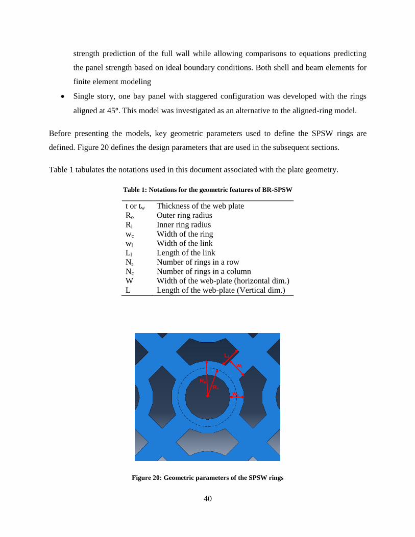
40

strength prediction of the full wall while allowing comparisons to equations predicting

the panel strength based on ideal boundary conditions. Both shell and beam elements for

finite element modeling

Single story, one bay panel with staggered configuration was developed with the rings

aligned at 45ᵒ. This model was investigated as an alternative to the aligned-ring model.

Before presenting the models, key geometric parameters used to define the SPSW rings are

defined. Figure 20 defines the design parameters that are used in the subsequent sections.

Table 1 tabulates the notations used in this document associated with the plate geometry.

Table 1: Notations for the geometric features of BR-SPSW

t or tw Thickness of the web plate

Ro Outer ring radius

Ri Inner ring radius

wc Width of the ring

wl Width of the link

Ll Length of the link

Nr Number of rings in a row

Nc Number of rings in a column

W Width of the web-plate (horizontal dim.)

L Length of the web-plate (Vertical dim.)

wl

Ll

wc

Rc

Ro

Figure 20: Geometric parameters of the SPSW rings

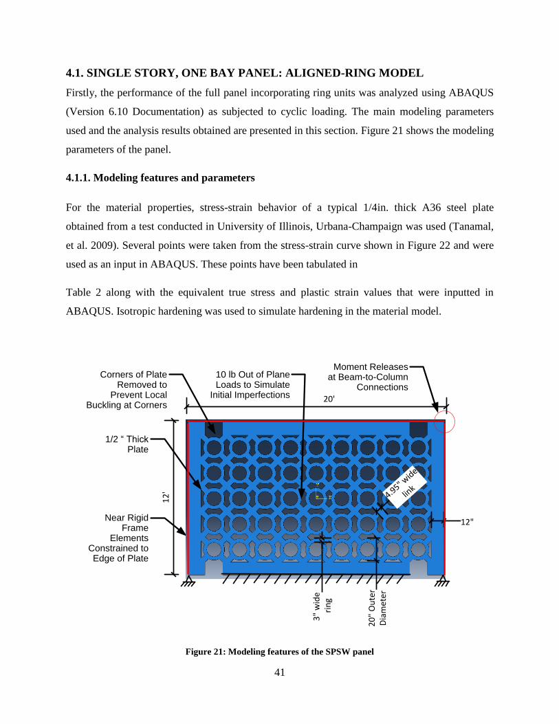
41

4.1. SINGLE STORY, ONE BAY PANEL: ALIGNED-RING MODEL

Firstly, the performance of the full panel incorporating ring units was analyzed using ABAQUS

(Version 6.10 Documentation) as subjected to cyclic loading. The main modeling parameters

used and the analysis results obtained are presented in this section. Figure 21 shows the modeling

parameters of the panel.

4.1.1. Modeling features and parameters

For the material properties, stress-strain behavior of a typical 1/4in. thick A36 steel plate

obtained from a test conducted in University of Illinois, Urbana-Champaign was used (Tanamal,

et al. 2009). Several points were taken from the stress-strain curve shown in Figure 22 and were

used as an input in ABAQUS. These points have been tabulated in

Table 2 along with the equivalent true stress and plastic strain values that were inputted in

ABAQUS. Isotropic hardening was used to simulate hardening in the material model.

12

'

20'

Near Rigid Frame

Elements Constrained to Edge of Plate

10 lb Out of Plane Loads to Simulate

Initial Imperfections

1/2 “ Thick Plate

20

" O

ute

rD

iam

eter

3"

wid

e r

ing

12"

Moment Releases at Beam-to-Column

Connections

Corners of Plate Removed to

Prevent Local Buckling at Corners

4.95" w

ide

link

Figure 21: Modeling features of the SPSW panel

42

Table 2: Engineering and true stress and strain values used for steel

Engineering

Stress (ksi)

Engineering

Strain(%)

True

stress(ksi)

Plastic

Strain (%)

40 0.35 40.14 0

40 0.8 40.32 0.65

47 2 47.94 1.81

50 3 57.5 2.77

61.4 15 70.61 13.73

Figure 22: Stress-strain behavior of the steel used for analysis

The Young’s Modulus (E) and the Poisson’s ratio for the steel has been taken as 29000 ksi and

0.3 respectively. The boundary elements have been modeled near rigid (Across-section= 5000 in2and

I=25e06 in4) with pinned connections to isolate the behavior of the shear wall. For meshing, four

node reduced integration (S4R) shell elements have been used and the meshing has been done

using an automatic meshing technique. A global approximate seeding size of 1.5 has been used.

To account for imperfections in the panel, several out-of-plane loads of 5 and 10 pounds were

applied to the panel at alternate rings on each row. Different types of boundary conditions were

applied on different sections of the model. Presented below is a brief description of all the

boundary conditions used.

The base of the plate was pinned.

0

10

20

30

40

50

60

70

0 5 10 15 20

En

gin

eeri

ng S

tres

s (k

si)

Engineering Strain (%)

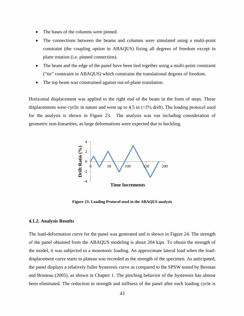
43

The bases of the columns were pinned.

The connections between the beams and columns were simulated using a multi-point

constraint (the coupling option in ABAQUS) fixing all degrees of freedom except in

plane rotation (i.e. pinned connection).

The beam and the edge of the panel have been tied together using a multi-point constraint

(“tie” constraint in ABAQUS) which constrains the translational degrees of freedom.

The top beam was constrained against out-of-plane translation.

Horizontal displacement was applied to the right end of the beam in the form of steps. These

displacements were cyclic in nature and went up to 4.5 in (≈3% drift). The loading protocol used

for the analysis is shown in Figure 23. The analysis was run including consideration of

geometric non-linearities, as large deformations were expected due to buckling.

Figure 23: Loading Protocol used in the ABAQUS analysis

4.1.2. Analysis Results

The load-deformation curve for the panel was generated and is shown in Figure 24. The strength

of the panel obtained from the ABAQUS modeling is about 204 kips. To obtain the strength of

the model, it was subjected to a monotonic loading. An approximate lateral load when the load-

displacement curve starts to plateau was recorded as the strength of the specimen. As anticipated,

the panel displays a relatively fuller hysteresis curve as compared to the SPSW tested by Berman

and Bruneau (2005), as shown in Chapter 1. The pinching behavior of the hysteresis has almost

been eliminated. The reduction in strength and stiffness of the panel after each loading cycle is

-4

-2

0

2

4

0 50 100 150 200

Dri

ft R

ati

o (

%)

Time Increments

44

minimal. Additionally, it can be observed from the hysteresis plot shown in Figure 24 that in the

first two cycles, there is a negligible lag in the lateral load resistance as the tension field reverses

direction, which is significantly less than that observed in a typical SPSW. The lag in the lateral

load resistance at the end of the third cycle is due to the plastic axial deformation of the rings and

links not dissimilar to the plastic axial deformations experienced in tests by Ciampi and

Samuelli-Ferretti (1990). It is expected that the plastic axial deformations and the resulting lag

in hysteretic behavior can be mitigated by adjusting the plate geometry. This will be investigated

as part of the parametric study.

Buckling observed in the plate deformed shape was consistent with global tension field type

buckling as shown in Figure 25. A small number of the rings experienced local lateral torsional

buckling. The maximum out-of-plane deformation at the end of the third cycle was recorded as 5

inches.

Figure 24: Hysteresis curve for the single story, one-bay panel.

The deformed shape of the panel and the stresses in the panel at 2% drift is shown in the Figure

25. A few important observations can be made from this figure. Note that the red color represents

yielded regions and the blue color represents regions below 35 ksi stress.

First, as noted earlier, a few links connecting the ring units are yielding. It is expected that

yielding of these links can be minimized by changing the plate geometry. Second, each ring

appears to develop four plastic hinges. This arrangement of plastic hinges forms the basis of the

plastic mechanisms derived in the next chapter to predict the strength of individual ring units.

-400

-300

-200

-100

0

100

200

300

400

-4 -2 0 2 4

Late

ral

Load

(k

ips)

Drift Ratio(%)

45

Figure 25: One bay, one story aligned ring panel at the 2% drift

4.2. SINGLE STORY, ONE-BAY PANEL: INFLUENCE OF DIAMETER OF THE

RINGS

To study the performance of the panel when the diameter of the rings is varied, two more models

were created in ABAQUS and their respective hysteresis curves were generated. Note that this

section describes a preliminary investigation of the effect of the ring diameter. A more rigorous

study is included in the later chapter on the parametric study.

Although BR-SPSW reduces the amount of buckling as compared to conventional steel plate

shear wall systems, it still buckles to some extent. In addition to the wall behavior (strength and

stiffness), this section also summarizes the preliminary investigation of the effect of ring

diameter on BR-SPSW buckling modes. This issue has been investigated in-depth in the

parametric study.

The basic ring unit dimensions of the panels tested as a part of this study is summarized in Table

3. All the other modeling parameters were identical to the model discussed in Section 4.1.

Table 3: Geometrical features of the panels to test the influence of the diameter

Ro Wc Wl

Panel 1 8 in. 2.4 in. 4.24 in.

Panel 2 16 in. 6 in. 9.9 in.

The hysteresis curves obtained from the analysis of Panel 1 are shown in Figure 26. As observed

from the hysteresis curve, Panel 1 exhibits stable and full hysteretic behavior up to the second

46

cycle. In the third cycle, the panel lags in lateral load resistance on tension field reversals, a

phenomenon also experienced by the previous panel. The strength for the panel was recorded as

212kips. Buckling of the panel was observed to be majorly global tension field buckling as

shown in Figure 26.

Figure 26: Hysteresis curve and out-of-plane deformation for Panel 1

Next, the hysteretic behavior of Panel 2 as captured and recorded in Figure 27. The panel

exhibits a full hysteretic behavior only up to 1% drift. Thereafter, some pinching can be observed

in the hysteresis curve. The strength of the panel was recorded as 359kips. Buckling of the panel

was mostly in the form of local lateral torsional buckling of the rings as shown in Figure 27.

A preliminary conclusion is that changing the diameter of the rings had a major effect on not

only the strength and the stiffness of the panel, but also on its buckling behavior. Ring size thus

appears to be a key geometrical feature of BR-SPSW. Additionally, two major modes of

buckling were identified: global tension field buckling and lateral torsional buckling of the rings.

The panels with larger radii were shown to exhibit a combination of the two modes and the

panels with smaller radii prominently exhibited global tension field buckling. It can also be noted

that a panel with a smaller diameter may result in a better hysteretic response with reduced

pinching.

-400

-300

-200

-100

0

100

200

300

400

-4 -2 0 2 4

Late

ral

Load

(k

ips)

Drift Ratio (%)

47

Figure 27: Hysteresis curve and out-of-plane deformation for Panel 2

This preliminary study on the influence of a parameter on the overall panel behavior was used to

inform the design of the parametric computational study, which is discussed in detail in Chapter

8.

4.3. UNCONSTRAINED RING MODEL

The unconstrained single ring configuration is used to isolate the smallest unit of BR-SPSW with

one end fixed and the other end subjected to horizontal displacement of up to 10 in. This model

was developed to capture the ring in its most unconstrained configuration in terms of boundary

conditions in the full wall. Figure 28 shows the unconstrained ring model with the boundary

conditions and applied displacement. This type of boundary condition was applied to models

using both shell and beam elements. The analysis results and conclusions are presented in the

subsequent sections.

4.3.1. Shell Model

The shell model was created using S4R elements in ABAQUS as shown in Figure 28. Outer

radius of the ring (Ro) for this model was chosen as 10 in. with a ring width (wc) of 3 inches.

Width of the link (wl) was set as 4.95 in. and thickness of the plate used was 0.5 in. Note that all

the material properties and the meshing techniques used were identical to that of the full wall.

-500

-400

-300

-200

-100

0

100

200

300

400

500

-4 -2 0 2 4

Late

ral

Load

(k

ips)

Drift Ratio (%)

48

Figure 28: Unconstrained ring model

The load - displacement curve obtained from the analysis is shown in Figure 29. The yield

strength predicted by the ABAQUS model is approximately 27 kips, as observed in the load-

deformation response by the sharp change in stiffness. The ring, however, exhibits increasing

post-yield strength which is a result of the geometric stiffening effect due to the forces in the

rings transitioning from flexural to axial at large deformations. This effect could be captured

because geometrical non-linearities were included in the analysis.

Figure 29: Load-displacement relationship for unconstrained ring shell model

To validate the results obtained from the mathematical solution regarding the transverse

shortening of the single ring unit, the elongation and shortening of the ring in the radial

directions were recorded. The results are plotted in

0

10

20

30

40

50

60

70

80

90

100

0 2 4 6 8

Rea

ctio

n (

kip

s)

Displacement (inches)

49

Figure 30, along with value of the transverse shortening predicted analytically in Section 3.

Figure 30: Comparison of effective Poisson’s ratio of the single ring unit

It is clear from the above plot that the ring has an effective Poisson’s ratio (PR) approximately

equal to 1.0 for small deformations which reinforces the fact that when a ring deforms into an

ellipse the longitudinal and transverse deformations are nearly same.

Note that the result obtained from ABAQUS is in agreement with the derivation done in Section

3 up to an elongation of 20% of the ring diameter (δ1/R=0.2). Under increasing elongation, the

ring behavior diverges from the analytical solution. It is expected that this is due to the inelastic

axial deformation which causes the perimeter of the ellipse to be larger than the original ring

perimeter.

4.3.2. Beam Model

The similar model using frame elements was created because it provides a more simplified

measurement of strength, as it eliminates the effect of the spread of plasticity through the width

of the ring. The model was created as a line model as shown in Figure 31, with a radius of 8.5 in.

Note that this is the centerline radius of the unconstrained ring model. The cross-sectional and

material properties assigned to the line model were identical to that used for shell element model

(t = 0.5 in., wc = 3 in., wl = 4.95 in.). Linear two node beam elements were used (B21 elements in

ABAQUS).

0

0.5

1

0 0.5 1Norm

ali

zed

tra

nsv

erse

def

orm

ati

on

(δ

2/R

)

Normalized longitudinal deformation

(δ1/R)

Abaqus data

PR=0.3

analytical result

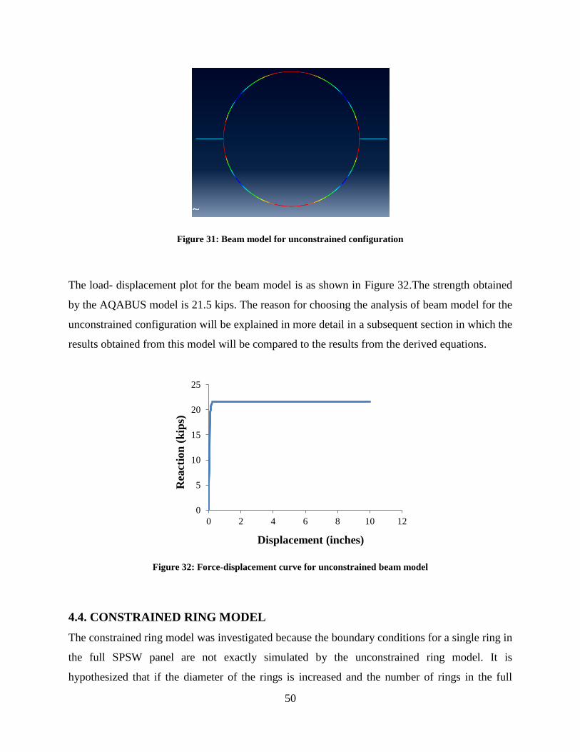
50

Figure 31: Beam model for unconstrained configuration

The load- displacement plot for the beam model is as shown in Figure 32.The strength obtained

by the AQABUS model is 21.5 kips. The reason for choosing the analysis of beam model for the

unconstrained configuration will be explained in more detail in a subsequent section in which the

results obtained from this model will be compared to the results from the derived equations.

Figure 32: Force-displacement curve for unconstrained beam model

4.4. CONSTRAINED RING MODEL

The constrained ring model was investigated because the boundary conditions for a single ring in

the full SPSW panel are not exactly simulated by the unconstrained ring model. It is

hypothesized that if the diameter of the rings is increased and the number of rings in the full

0

5

10

15

20

25

0 2 4 6 8 10 12

Rea

ctio

n (

kip

s)


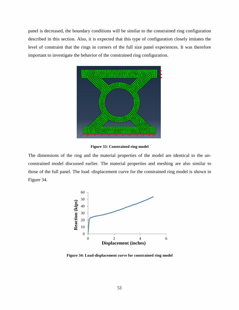
51

panel is decreased, the boundary conditions will be similar to the constrained ring configuration

described in this section. Also, it is expected that this type of configuration closely imitates the

level of constraint that the rings in corners of the full size panel experiences. It was therefore

important to investigate the behavior of the constrained ring configuration.

Figure 33: Constrained ring model

The dimensions of the ring and the material properties of the model are identical to the un-

constrained model discussed earlier. The material properties and meshing are also similar to

those of the full panel. The load -displacement curve for the constrained ring model is shown in

Figure 34.

Figure 34: Load-displacement curve for constrained ring model

0

10

20

30

40

50

60

0 2 4 6

Rea

ctio

n (

kip

s)


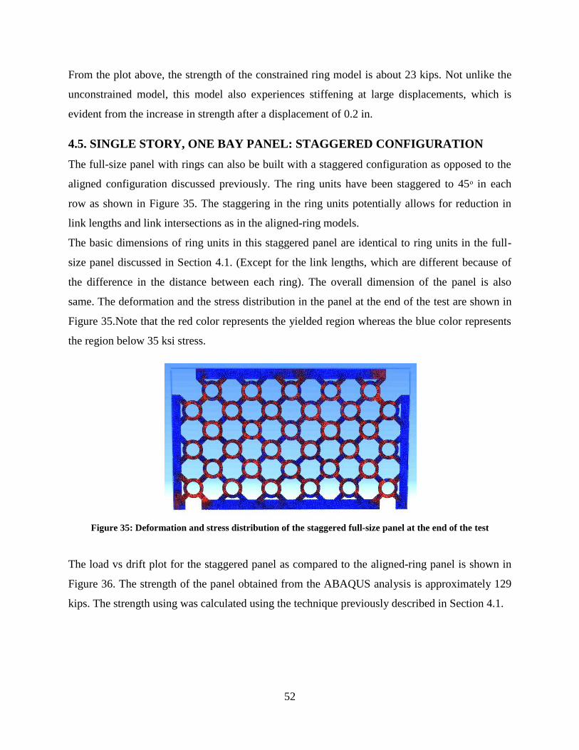
52

From the plot above, the strength of the constrained ring model is about 23 kips. Not unlike the

unconstrained model, this model also experiences stiffening at large displacements, which is

evident from the increase in strength after a displacement of 0.2 in.

4.5. SINGLE STORY, ONE BAY PANEL: STAGGERED CONFIGURATION

The full-size panel with rings can also be built with a staggered configuration as opposed to the

aligned configuration discussed previously. The ring units have been staggered to 45ᵒ in each

row as shown in Figure 35. The staggering in the ring units potentially allows for reduction in

link lengths and link intersections as in the aligned-ring models.

The basic dimensions of ring units in this staggered panel are identical to ring units in the full-

size panel discussed in Section 4.1. (Except for the link lengths, which are different because of

the difference in the distance between each ring). The overall dimension of the panel is also

same. The deformation and the stress distribution in the panel at the end of the test are shown in

Figure 35.Note that the red color represents the yielded region whereas the blue color represents

the region below 35 ksi stress.

Figure 35: Deformation and stress distribution of the staggered full-size panel at the end of the test

The load vs drift plot for the staggered panel as compared to the aligned-ring panel is shown in

Figure 36. The strength of the panel obtained from the ABAQUS analysis is approximately 129

kips. The strength using was calculated using the technique previously described in Section 4.1.

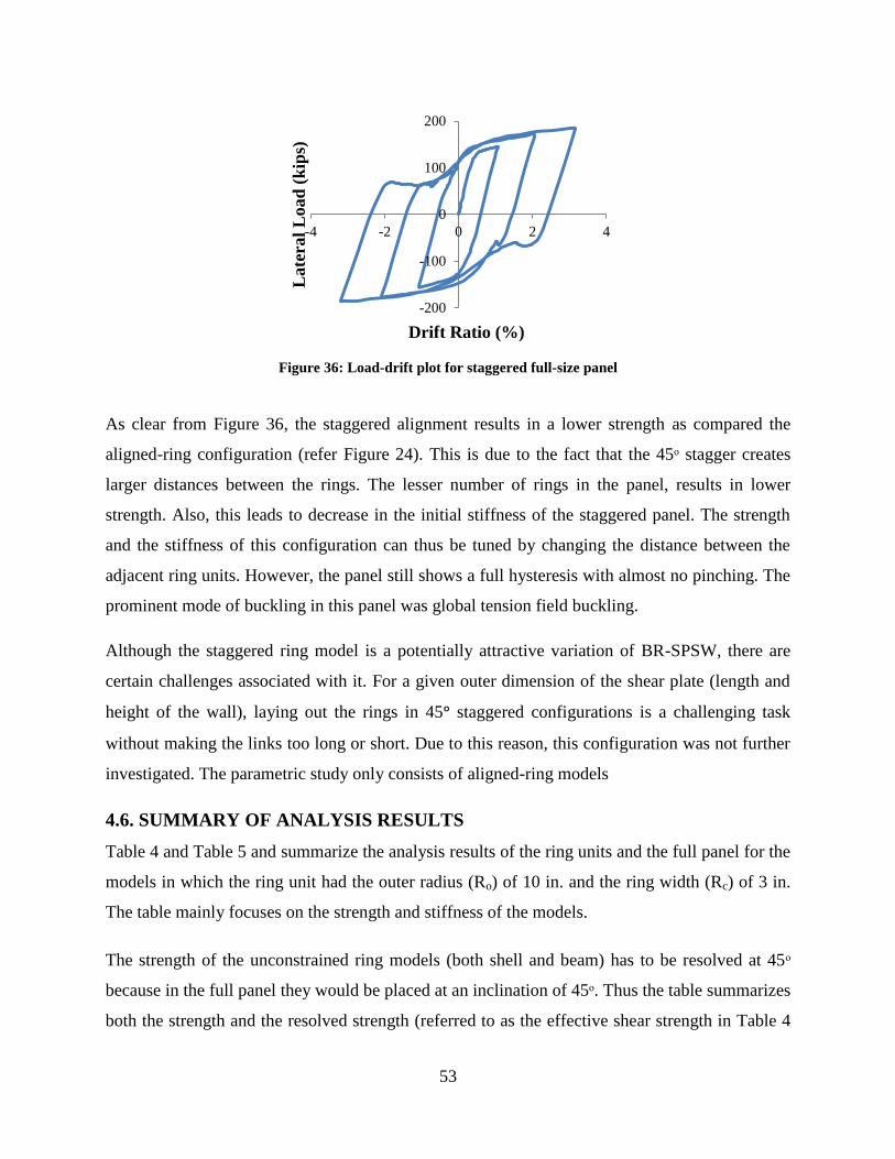
53

Figure 36: Load-drift plot for staggered full-size panel

As clear from Figure 36, the staggered alignment results in a lower strength as compared the

aligned-ring configuration (refer Figure 24). This is due to the fact that the 45ᵒ stagger creates

larger distances between the rings. The lesser number of rings in the panel, results in lower

strength. Also, this leads to decrease in the initial stiffness of the staggered panel. The strength

and the stiffness of this configuration can thus be tuned by changing the distance between the

adjacent ring units. However, the panel still shows a full hysteresis with almost no pinching. The

prominent mode of buckling in this panel was global tension field buckling.

Although the staggered ring model is a potentially attractive variation of BR-SPSW, there are

certain challenges associated with it. For a given outer dimension of the shear plate (length and

height of the wall), laying out the rings in 45ᵒ staggered configurations is a challenging task

without making the links too long or short. Due to this reason, this configuration was not further

investigated. The parametric study only consists of aligned-ring models

4.6. SUMMARY OF ANALYSIS RESULTS

Table 4 and Table 5 and summarize the analysis results of the ring units and the full panel for the

models in which the ring unit had the outer radius (Ro) of 10 in. and the ring width (Rc) of 3 in.

The table mainly focuses on the strength and stiffness of the models.

The strength of the unconstrained ring models (both shell and beam) has to be resolved at 45ᵒ

because in the full panel they would be placed at an inclination of 45ᵒ. Thus the table summarizes

both the strength and the resolved strength (referred to as the effective shear strength in Table 4

-200

-100

0

100

200

-4 -2 0 2 4

Late

ral

Load

(k

ips)

Drift Ratio (%)

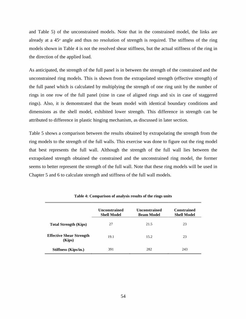
54

and Table 5) of the unconstrained models. Note that in the constrained model, the links are

already at a 45ᵒ angle and thus no resolution of strength is required. The stiffness of the ring

models shown in Table 4 is not the resolved shear stiffness, but the actual stiffness of the ring in

the direction of the applied load.

As anticipated, the strength of the full panel is in between the strength of the constrained and the

unconstrained ring models. This is shown from the extrapolated strength (effective strength) of

the full panel which is calculated by multiplying the strength of one ring unit by the number of

rings in one row of the full panel (nine in case of aligned rings and six in case of staggered

rings). Also, it is demonstrated that the beam model with identical boundary conditions and

dimensions as the shell model, exhibited lower strength. This difference in strength can be

attributed to difference in plastic hinging mechanism, as discussed in later section.

Table 5 shows a comparison between the results obtained by extrapolating the strength from the

ring models to the strength of the full walls. This exercise was done to figure out the ring model

that best represents the full wall. Although the strength of the full wall lies between the

extrapolated strength obtained the constrained and the unconstrained ring model, the former

seems to better represent the strength of the full wall. Note that these ring models will be used in

Chapter 5 and 6 to calculate strength and stiffness of the full wall models.

Table 4: Comparison of analysis results of the rings units

Unconstrained

Shell Model

Unconstrained

Beam Model

Constrained

Shell Model

Total Strength (Kips) 27 21.5 23

Effective Shear Strength

(Kips) 19.1 15.2 23

Stiffness (Kips/in.) 391 282 243

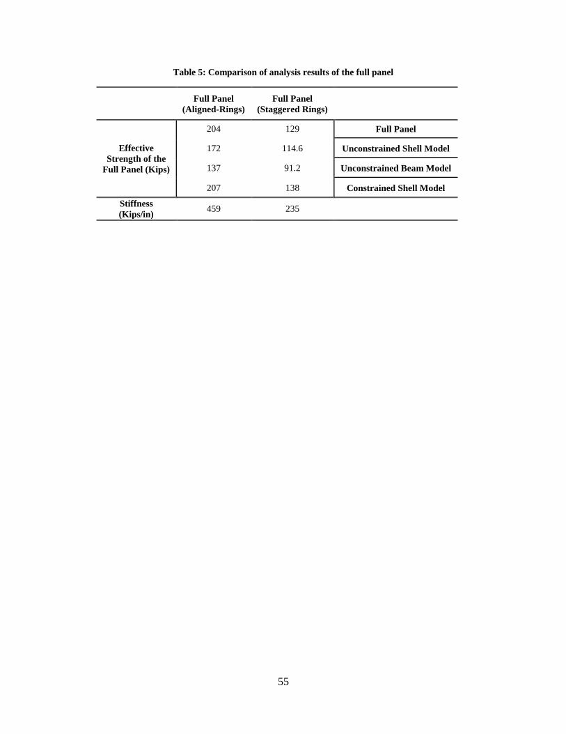
55

Table 5: Comparison of analysis results of the full panel

Full Panel

(Aligned-Rings)

Full Panel

(Staggered Rings)

Effective

Strength of the

Full Panel (Kips)

204 129 Full Panel

172 114.6 Unconstrained Shell Model

137 91.2 Unconstrained Beam Model

207 138 Constrained Shell Model

Stiffness

(Kips/in) 459 235

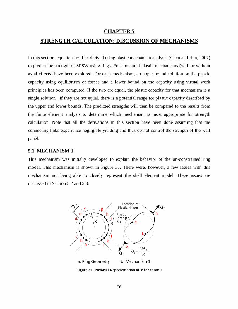
56

CHAPTER 5

STRENGTH CALCULATION: DISCUSSION OF MECHANISMS

In this section, equations will be derived using plastic mechanism analysis (Chen and Han, 2007)

to predict the strength of SPSW using rings. Four potential plastic mechanisms (with or without

axial effects) have been explored. For each mechanism, an upper bound solution on the plastic

capacity using equilibrium of forces and a lower bound on the capacity using virtual work

principles has been computed. If the two are equal, the plastic capacity for that mechanism is a

single solution. If they are not equal, there is a potential range for plastic capacity described by

the upper and lower bounds. The predicted strengths will then be compared to the results from

the finite element analysis to determine which mechanism is most appropriate for strength

calculation. Note that all the derivations in this section have been done assuming that the

connecting links experience negligible yielding and thus do not control the strength of the wall

panel.

5.1. MECHANISM-I

This mechanism was initially developed to explain the behavior of the un-constrained ring

model. This mechanism is shown in Figure 37. There were, however, a few issues with this

mechanism not being able to closely represent the shell element model. These issues are

discussed in Section 5.2 and 5.3.

ab

c

de

f gh

i

jk

l b

e

h

k

R

Plastic Strength, Mp

a. Ring Geometry b. Mechanism 1

1

4 pMQ

R

Location of Plastic HingeswL

Q1

Q1

Figure 37: Pictorial Representation of Mechanism I

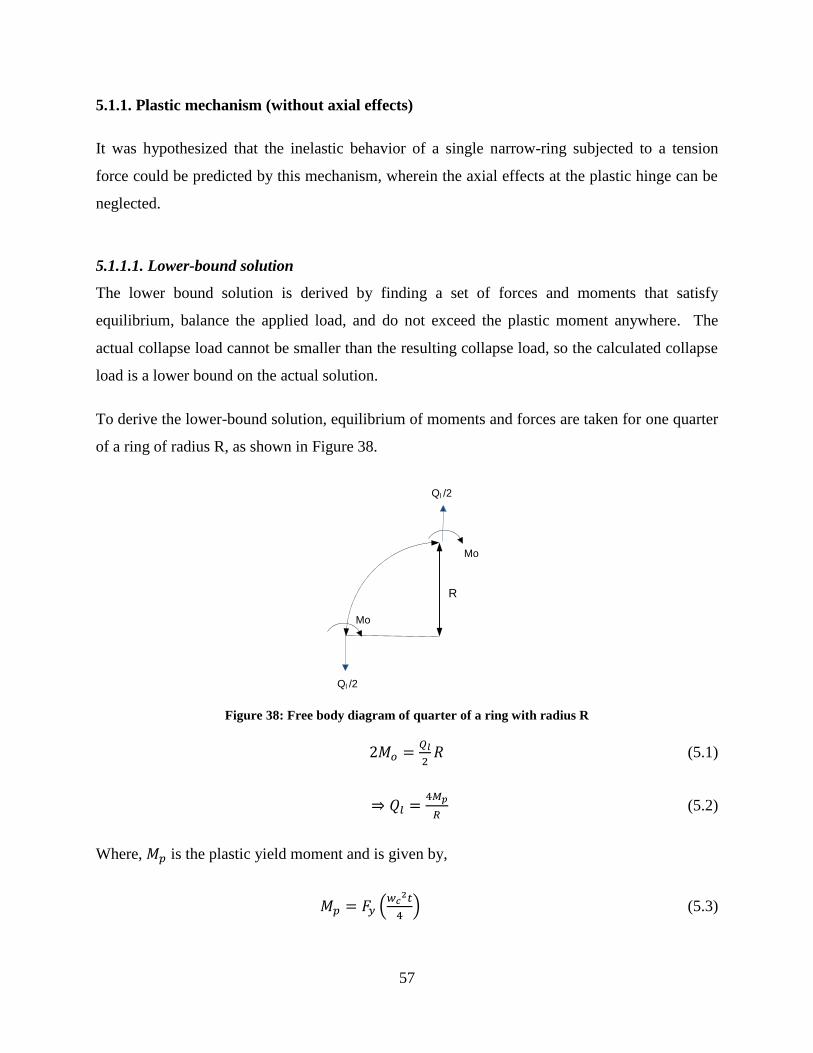
57

5.1.1. Plastic mechanism (without axial effects)

It was hypothesized that the inelastic behavior of a single narrow-ring subjected to a tension

force could be predicted by this mechanism, wherein the axial effects at the plastic hinge can be

neglected.

5.1.1.1. Lower-bound solution

The lower bound solution is derived by finding a set of forces and moments that satisfy

equilibrium, balance the applied load, and do not exceed the plastic moment anywhere. The

actual collapse load cannot be smaller than the resulting collapse load, so the calculated collapse

load is a lower bound on the actual solution.

To derive the lower-bound solution, equilibrium of moments and forces are taken for one quarter

of a ring of radius R, as shown in Figure 38.

90

Ql /2

Ql /2

Mo

Mo

R

Figure 38: Free body diagram of quarter of a ring with radius R

(5.1)

(5.2)

Where, is the plastic yield moment and is given by,

(

) (5.3)

58

In the above equation, is the yield stress of the material, is the width of the ring and is the

thickness of the steel plate used.

5.1.1.2. Upper-bound solution

The upper-bound solution is derived based on a compatible pattern of plastic deformations. The

associated collapse load is computed using virtual work whereby the rate of work done by the

external forces equals the rate of internal energy dissipation. Since the actual collapse load

cannot be lower than the collapse load calculated in this way, the computed collapse load is an

upper bound on the actual collapse load.

Consider the centerline of the ring with plastic hinges as shown in Figure 39.

R

√2 R

R

b

a c

d

Plastic

Hinge

Figure 39: Plastic Hinge mechanism without axial effects

After the formation of plastic hinges, the arcs ab, bc, cd and da will rotate about the plastic

hinges as shown in the Figure 40.

External work done, We, by load Q is given by:

(5.4)

Where is the displacement of the point “c”. Note that Point “a” is fixed.

Internal work, Wi, done by the plastic moment at the plastic hinges is given by:

(5.5)

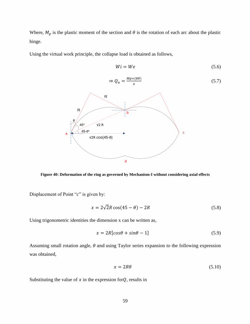
59

Where, is the plastic moment of the section and is the rotation of each arc about the plastic

hinge.

Using the virtual work principle, the collapse load is obtained as follows,

(5.6)

(5.7)

R

R

√2 R

√2R cos(45-θ)

45ᵒ

θ

45-θᵒa

b

d

c

Figure 40: Deformation of the ring as governed by Mechanism-I without considering axial effects

Displacement of Point “c” is given by:

√ (5.8)

Using trigonometric identities the dimension x can be written as,

[ ] (5.9)

Assuming small rotation angle, using Taylor series expansion to the following expression

was obtained,

(5.10)

Substituting the value of in the expression for , results in

60

(5.11)

Since the lower-bound solution is the same as upper-bound solution, the collapse load is obtained

as,

(5.12)

5.1.2. Plastic mechanism with axial effects

In this mechanism the inelastic axial deformations are considered. This mechanism was

examined to explain the behavior of the wide-ring unconstrained model as the axial effects are

significant and cannot be neglected in wider rings. The concept is shown in the deformed ring

shown in Figure 41.

Plastic Hinge

Plastic axial

deformation

Figure 41: Plastic mechanism with axial effects

The cross-section used for the ring is a rectangular section. Thus the axial-bending interaction

curve is approximately shown in Figure 42:

Mathematically, the curve can be expressed as follows:

(

)

(5.13)

61

M/Mo , Mo ǿ

N/No , No ἐ

Strain Rate

1.0

-1.0

-1.0 1.0

Figure 42: axial-bending interaction curve for rectangular cross-section [from (Chen and Han 2007)]

The plastic flow rule requires the generalized plastic strain rate vector to be normal to the plastic

potential surface (assumed to be the same as the yield surface) at all points where the normal is

uniquely defined. Thus,

(5.14)

(5.15)

Going back to the geometry of the deformed circle, and relating it to the axial-bending

interaction curve it is noted that energy dissipation/unit length at Points a and b is given by:

(5.16)

(5.17)

5.1.2.1. Upper-bound solution

As mentioned in the discussion for the previous mechanism, the solution for the collapse load

will be done in the form of lower-bound and upper-bound. Starting with the upper-bound

solution, the internal work done by the plastic moment and the external work done by the applied

force has been evaluated as follows.

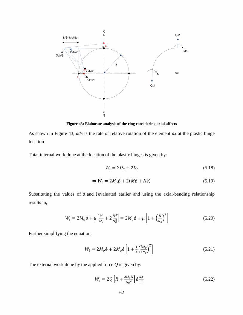
62

Q

Q

Ǿdx/2

Ǿdx/2

ἐ/ǿ=Mo/No

ἐ dx/2

RǾdx/2

R

a

b

90

Q/2

Q/2

Mo

M

Figure 43: Elaborate analysis of the ring considering axial affects

As shown in Figure 43, ǿdx is the rate of relative rotation of the element dx at the plastic hinge

location.

Total internal work done at the location of the plastic hinges is given by:

(5.18)

(5.19)

Substituting the values of and evaluated earlier and using the axial-bending relationship

results in,

[

] [ (

)

] (5.20)

Further simplifying the equation,

[

(

)

] (5.21)

The external work done by the applied force Q is given by:

[

]

(5.22)

63

Using the virtual work Principle,

(5.23)

On simplifying the equation,

[

(

) (

) ]

(5.24)

To obtain maximum Q for a given ratio of , differentiate Q with respect to

(

) (5..25)

On differentiating and simplifying a quadratic equation in is obtained.

(

)

(

) (

)

(5.26)

Solving the quadratic equation,

[ √

(

)

] (5.27)

The resulting upper bound plastic capacity is given by Equation 5.24 with the value for strain

rate ratio from Equation 5.27 substituted in.

5.1.2.2. Lower-Bound Solution

For lower-bound solution, the equilibrium of moments and forces was considered as shown in

Figure 43.

(5.28)

Since axial-bending interaction curve for a rectangular cross-section has been used,

(

)

(5.29)

Here,

64

(5.30)

Hence,

(

)

(5.31)

The two equations were combined to get a quadratic in Q,

(

)

(

) (5.32)

Solving for Q,

√(

)

(5.33)

On comparing the upper and the lower bounds of the collapse load, it was found that they do not

give the same result. Thus, the collapse load for this mechanism is found to be within the range

between the upper and lower bounds. Note that for comparison of results from ABAQUS and

predicted strength from equations later in this section, the upper-bound solution of this

mechanism has been used for simplicity.

5.2. MECHANISM-II

Note that the plastic mechanisms in the previous two sections assumed the ring as a circle using

the centerline radius R with four plastic hinges. The unconstrained ring in the ABAQUS model

however has a link width wc which spreads out the plastic hinge at the locations of the load

application. The spread of plasticity at the points of load application is not captured in the

previous two mechanisms. To account for the width of the link at the location of load

application, a slight modification to Mechanism I, was devised in an attempt to better simulate

the behavior of the unconstrained ring model.

For this mechanism, the position of the plastic hinges was represented as shown in the Figure 44.

Note that radius of the circle represented by Rc is the centerline radius of the ring model and that

axial yielding is neglected for this mechanism

65

W

l

Rc

Q Q

Figure 44: Line diagram for Mechanism -II

This mechanism better represents the plastic hinging in the un-constrained ring model as is clear

from its stress distribution diagram shown in Figure 45. As previously described in Chapter 4,

the Von Mises stress distribution in an unconstrained ring model reflects a certain pattern of

plastic yielding. Note that the red and the orange region represent the yielded region and the blue

region represents the zones with less than 13 ksi stress.

Figure 45: Stress distribution in an un-constrained ring (red and orange regions are yielded)

Wl

Rc

≈ Rc

Rc-wl/2θ

a

b

Figure 46: Dimensional features of Mechanism-II

66

As observed from the figure, instead of one plastic hinge at the joint of the ring and link, the

stress pattern shows two distinct plastic hinges at each side of the link. Thus, Figure 44 and

Figure 46 better simulates the behavior of the unconstrained ring model.

5.2.1. Lower-Bound Solution

Consider the equilibrium of forces and moments in the arc “ab” about point “b” as shown in

Figure 47. The lower bound plastic capacity is computed as follows.

90

Q/2

Q/2

Mo

Mo

Rc-wl/2

Figure 47: Free body diagram of quarter of a ring (Mechanism-II)

(5.34)

(5.35)

5.2.2. Upper-Bound Solution

After the formation of plastic hinge, the arcs ab, bc, cd and da will rotate about the plastic hinges

as shown in Figure 48:

External work, We, done by load Q is given by:

(5.36)

Where is the displacement of the point “c”. Note that Point “a” is fixed.

Internal work, Wi, done by the plastic moment at the plastic hinges is given by:

(5.37)

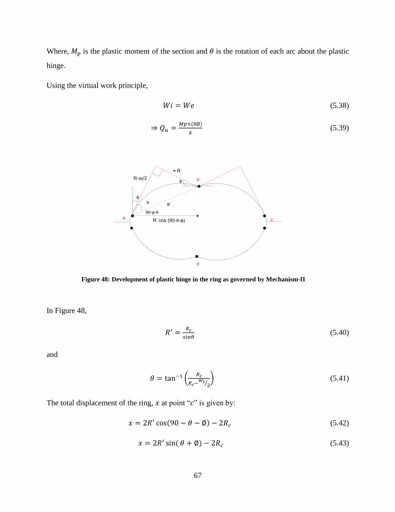
67


hinge.

Using the virtual work principle,

(5.38)

(5.39)

R’

R’ cos (90-θ-φ)

θ

φ

90-φ-θ

φ

≈ R

R-wl/2

a

b

d

c

Figure 48: Development of plastic hinge in the ring as governed by Mechanism-II

In Figure 48,

(5.40)

and

(

⁄) (5.41)

The total displacement of the ring, at point “c” is given by:

(5.42)

(5.43)

68

Using trigonometric identities and assuming a small φ,

(5.44)

Substituting the value of R’ and simplifying to the total displacement,

(5.45)

(5.46)

Substituting this value of in the expression for results in,

(5.47)

Since the lower-bound solution is the same as upper-bound solution, the collapse load is obtained

as,

(5.48)

(5.49)

where,

(5.50)

Thus, it can be concluded that a better prediction of the strength of the unconstrained ring can be

made by slightly modifying the effective radius of the ring.

5.3. MECHANISM-III

Another mechanism was developed on observing the deformation of individual ring units in the

full-size panel wall. The magnified deformed ring and the mechanism are shown in Figure 49.

69

Rc-wl/2

Rc-wl/2

Figure 49: idealized line-diagram for Mechanism-III

It can be proved that the strength predicted by this mechanism is identical to that predicted by

Mechanism II.

The total displacement of the ring at point “d” shown in Figure 50 is given by:

(5.51)

√ (

⁄ ) (5.52)

R’

R’ cos (45-θ)

45ᵒ

θ

45-θ

θR-wl/2

a

b

d

c

f e

R-wl/2

wl

Figure 50: Deformation of the ring as governed by Mechanism-III

Using trigonometric identities the total displacement of the ring at point “d” can be calculated

as:

70

(

⁄ )[ ] (5.53)

Assuming θ is small and using Taylor series expansion,

(

⁄ )[ ] (5.54)

⁄ (5.55)

Computing the internal work done by the plastic moment to the external work done by the

applied force, as done in all the previous derivations, results in external work done by load Q is

given by:

(5.56)

Where is the displacement of the point “d”. Note that Point “a” is fixed.

Internal work done by the plastic moment at the plastic hinges is given by:

(5.57)


hinge.


(5.58)

(5.59)

Substituting this value of in the expression for ,

(5.60)

The same solution can be obtained for the lower-bound by taking the equilibrium of moments

and forces for quarter of the ring (between two plastic hinges).

Thus, the collapse load for this mechanism is identical to that of Mechanism-II and is given by:

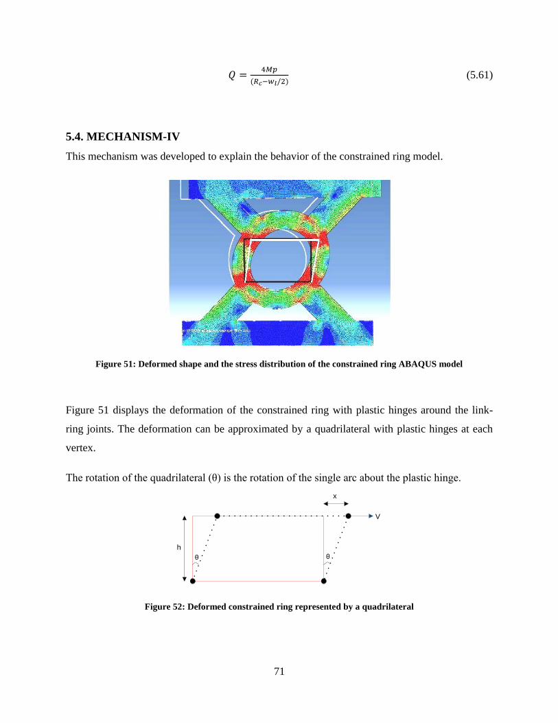
71

(5.61)

5.4. MECHANISM-IV

This mechanism was developed to explain the behavior of the constrained ring model.

Figure 51: Deformed shape and the stress distribution of the constrained ring ABAQUS model

Figure 51 displays the deformation of the constrained ring with plastic hinges around the link-

ring joints. The deformation can be approximated by a quadrilateral with plastic hinges at each

vertex.

The rotation of the quadrilateral (θ) is the rotation of the single arc about the plastic hinge.

θ θ

h

x

V

Figure 52: Deformed constrained ring represented by a quadrilateral

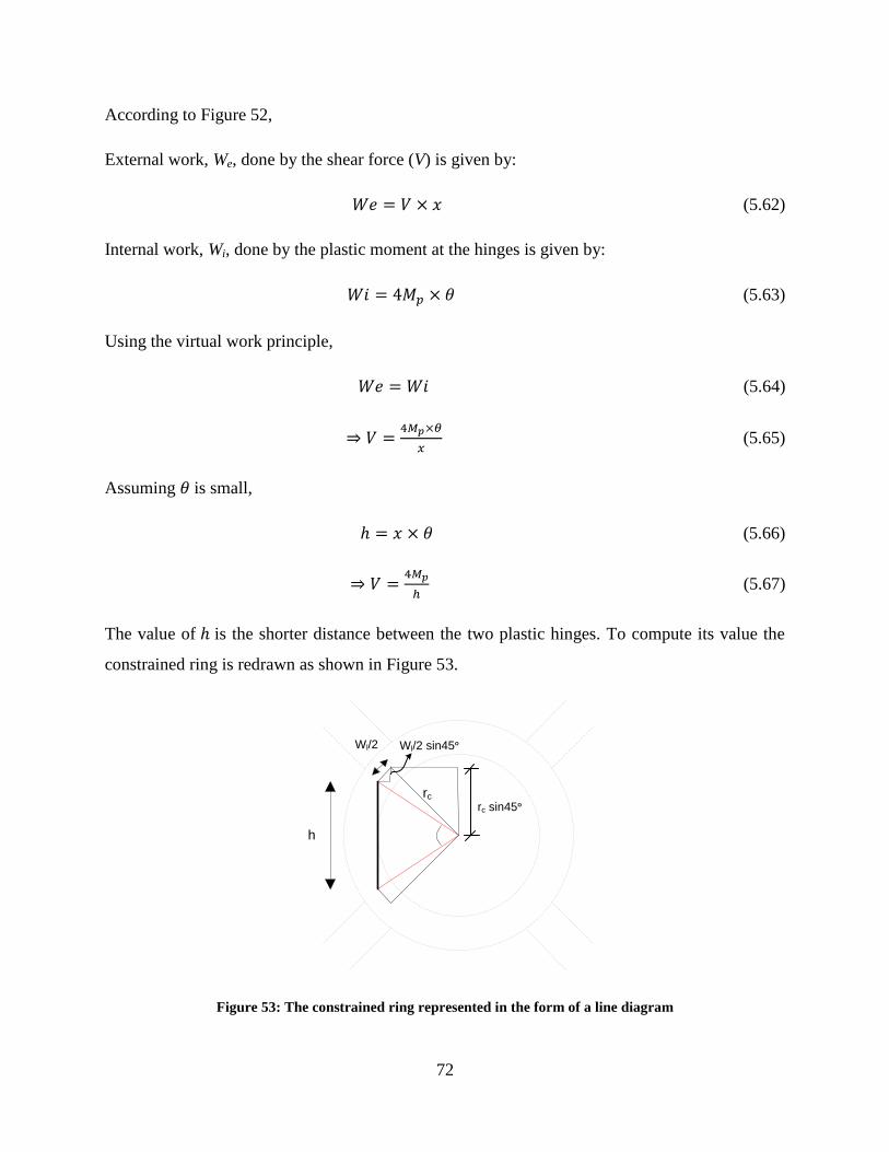
72

According to Figure 52,

External work, We, done by the shear force (V) is given by:

(5.62)

Internal work, Wi, done by the plastic moment at the hinges is given by:

(5.63)


(5.64)

(5.65)

Assuming is small,

(5.66)

(5.67)

The value of is the shorter distance between the two plastic hinges. To compute its value the

constrained ring is redrawn as shown in Figure 53.

h

Wl/2

rc

rc sin45ᵒ

Wl/2 sin45ᵒ

Figure 53: The constrained ring represented in the form of a line diagram

73

Here,

(5.68)

√

(5.69)

Where, is the center-line radius of the ring and is the centerline radius of the ring.

Using this value of to compute V,

√ (5.70)

5.5. COMPARISON OF RESULTS

This section focuses on investigating the effectiveness of the derived equations in predicting the

strength of ring models and the full panels from the preliminary study. Thus, this section is an

extension to the comparison of analysis results of the various ABAQUS models done in Chapter

4. The results from ABAQUS analysis done for the preliminary study have been compared to the

predicted strength in a set of tables presented below.

For extrapolating the plastic capacity of the ring to the capacity of the full panel, strength/ring is

multiplied by the number of rings in a row to get the approximate strength of the full wall. An

important thing to be pointed out in the table is the fact that for the unconstrained ring model, the

strength has been calculated along the connecting links. When these rings become a part of the

full panel the links are aligned at 45ᵒ and thus the total strength of the rings is required to be

resolved in the horizontal direction to get the effective strength of the panel.

Comparing the results in Table 6 and Table 7, it was observed that Mechanism-II/III and IV very

well predict the strength of the unconstrained and constrained shell model respectively.

However, the main conclusion that can be drawn from Table 8 and Table 9 is that the strength of

the full-panel is very well predicted by the constrained shell model as the average strength of the

ring in the full panel is almost equal to the constrained ring model. The unconstrained models

also give good results but they are not as close to the predicted results as the constrained model.

74

Another point to be noticed from the comparison is that in most of the cases axial effects do not

have a significant influence in the strength of the models (refer Table 6).

Thus, based on the previous conclusion, Mechanism IV (constrained ring model) has been used

for BR-SPSW strength calculation from this point onwards. The accuracy of the analytical

solution (Mechanism-IV) in predicting the strength of the full wall specimens analyzed in the

parametric study is investigated in Chapter 8.

Table 6: Comparison of computational and analytical results for unconstrained models

Calculated Plastic Capacity (kips) Observed Strength From FEM Model

Mechanism I Mechanism II Mechanism III Shell Model Beam Model

No Axial Effects 21.2 29.8 29.8

27.0 kips 23.0 kips Axial Effects

Included 21.1 28.4 28.4

Table 7: Comparison of computational and analytical results for constrained model

Constrained

Ring

Calculated Plastic Capacity Observed Strength From FEM Model

Mechanism IV Shell Elements

22.3 kips 23.0 kips

Table 8: Comparison of computational and analytical results for full wall models

Calculated Plastic Capacity (kips) Observed

Strength from full

wall (FEM Model) Mechanism II Mechanism III Mechanism IV

Single Story

Panel 172 172 201 204 kips

Table 9: Comparison of results obtained from Mechanism-IV to computational results

Calculated

Plastic Cap. Observed Strength From FEM Model (kips)

Mechanism IV

Unconstrained

Ring with Shell

Elements

Unconstrained

Ring Frame

Elements

Constrained

Ring

Full Panel /

Number of

Rings

Shear Strength

/Ring 22.3 19.1 15.2 23.0 22.6

75

CHAPTER 6

STIFFNESS CALCULATION: DISCUSSION OF MECHANISMS

This section develops the analytical solution for the stiffness of the full wall panel. The geometry

of the BR-SPSW makes the derivation for stiffness quite challenging. To simplify the problem, a

single ring unit and its deformation mechanics was considered to derive the analytical solution.

The problem has been solved using two types of single ring unit models. A detailed derivation of

stiffness using both these models and the assumptions associated with them is presented in the

subsequent paragraphs.

6.1. UNCONSTRAINED RING MODEL

Consider the unconstrained ring model subjected to a point load P as shown in Figure 54. Note

that since the axial stiffness of the connecting links (transferring the load P to the ring) is much

larger than the total stiffness of the ring, link stiffness was ignored while deriving the stiffness of

the unconstrained ring model.

A B

D

C

D

C

A B

N

MxV

P/2

Mo

θ

R

P

P

Figure 54: Unconstrained ring model

From symmetry, the deformations of each quadrant of the ring are identical. Hence, only one

quadrant, ABCD, has been considered. The quadrant has been considered fixed at the section DC

with a load P/2 and moment Mo at section AB. Because of the symmetry of the ring and ring

76

deformations, section AB always remains perpendicular to section DC. Thus, the rotation of face

AB is zero. Using Castigliano’s Theorem it can be proved that (Boresi and Schmidt, 2003).

(

) (6.1)

where, R is the centerline radius of the ring; A is the cross sectional area and Am for the ring

cross-section is given by:

(6.2)

where, t is the thickness of the ring; Ro and Ri are the outer and the inner radius of the ring

respectively.

For quadrant ABCD, the shear force (V), normal force (Nx) and bending moment (Mx) acting on

a section at an angle θ can be expressed as:

(6.3)

(6.4)

(6.5)

(

) (6.6)

Castigliano’s Theorem was used to find the vertical deflection (δ) of the quadrant ABCD, due to

applied load P/2.

⁄ (6.7)

∫

⁄ ∫

⁄ ∫

⁄ (6.8)

where, E,I,G and κ are the material and geometric properties of the ring and dz is an infinitesimal

section of the ring and can be expressed as Rdθ. Substituting the expression for dz integrating the

expression from 0 to π/2,

77

(

{

}) (6.9)

The stiffness of the quadrant ABCD, is thus given by the expression,

(

{

})

(6.10)

where,

(6.11)

Thus, the ring has four quadrants each with stiffness Ku as shown in the Figure 55. Effective

stiffness of the ring can be calculated by considering the series and parallel stiffness combination

of each quadrant as shown in figure. Thus, the resultant stiffness of the ring was obtained as Ku.

Ku

KuKu

Ku

Ku/2

Ku/2

≡ ≡

Ku

Figure 55: Resultant stiffness of the ring

As mentioned previously, the axial stiffness of the links is believed to have negligible effect on

the stiffness of the ring model. As shown in Figure 55, the stiffness of the links will act in series

with the stiffness of the ring. Since the axial stiffness of the link is very large as compared to the

stiffness of the ring, the resultant stiffness (K) is almost equal to the stiffness of the ring by itself.

(6.11)

Based on the stiffness of the unconstrained ring model, the stiffness of the full wall has been

calculated. The stiffness of full wall (Kw) has been expressed in terms of number of rings in a

column (Nc), number of rings in a row (Nr) and stiffness of one ring based on unconstrained ring

model (ku).

78

Inclined array

N full

Δ=1

F1 F2 FNr-1

Δ=1/√2

Figure 56: Stiffness of the full wall

From Figure 56,

Number of inclined arrays (N) = Nc+ Nr -1

Number of inclined arrays with maximum number of rings (Nfull) = N- 2(Nr-1) = Nc –Nr+1

Resultant stiffness of the inclined array (kc’) along its length is given by,

(6.12)

To calculate the stiffness of the full panel, it was subjected to a unit horizontal displacement as

shown in Figure 56. Force experienced by each inclined array along its length due to this

horizontal displacement is given by F1, F2, ….FN. Firstly, the forces experienced by the partial

arrays (denoted by dotted lines in the Figure 56) have been considered.

When the panel is being subjected to a unit displacement in the horizontal direction, each array is

only experiencing a fraction of the displacement. As shown in the Figure 57, array AB is only

experiencing a displacement equal to the difference of the horizontal displacement of its top and

bottom end (A and B) which is given by,

79

(6.13)

Δ=1

Δ=Nr-1/Nr

Δ=Nr-2/Nr

Δ=1/Nr

A

B

C

D

Figure 57: Displacement of inclined arrays

This horizontal displacement is then resolved along the array length to calculate the force in the

array along its length.

√ (6.14)

√ √

(6.15)

Similarly for other arrays,

√ √

√

(6.16 a)

.

.

.

.

√ √

√

(6.16 i)

Note that each force has been multiplied by a factor of 2 to account for an identical array

positioned in the opposite corner of the full panel.

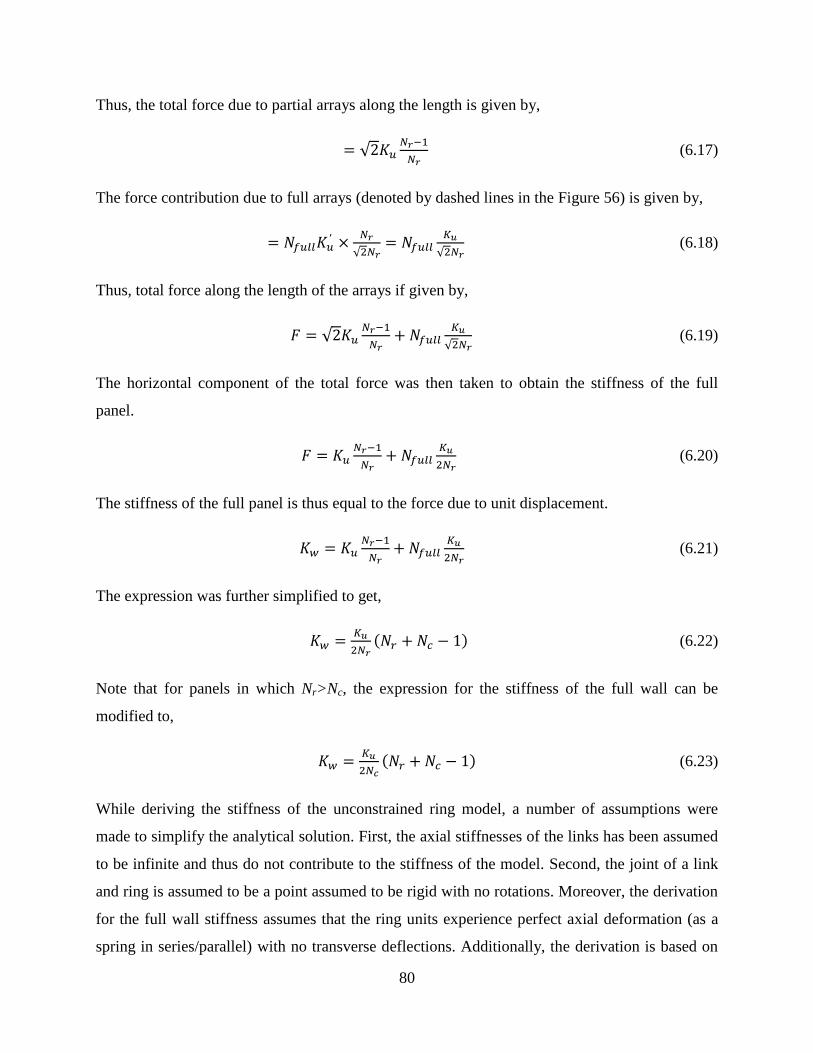
80

Thus, the total force due to partial arrays along the length is given by,

√

(6.17)

The force contribution due to full arrays (denoted by dashed lines in the Figure 56) is given by,

√

√ (6.18)

Thus, total force along the length of the arrays if given by,

√

√ (6.19)

The horizontal component of the total force was then taken to obtain the stiffness of the full

panel.

(6.20)

The stiffness of the full panel is thus equal to the force due to unit displacement.

(6.21)

The expression was further simplified to get,

(6.22)

Note that for panels in which Nr>Nc, the expression for the stiffness of the full wall can be

modified to,

(6.23)

While deriving the stiffness of the unconstrained ring model, a number of assumptions were

made to simplify the analytical solution. First, the axial stiffnesses of the links has been assumed

to be infinite and thus do not contribute to the stiffness of the model. Second, the joint of a link

and ring is assumed to be a point assumed to be rigid with no rotations. Moreover, the derivation

for the full wall stiffness assumes that the ring units experience perfect axial deformation (as a

spring in series/parallel) with no transverse deflections. Additionally, the derivation is based on

81

the Castigliano’s theorem as the initial premise which implies that it is only valid in the linear

elastic region for a material. The comparison of the predicted stiffness with the results obtained

from FE modeling is done in Chapter 8.

6.2. CONSTRAINED RING MODEL

Consider the constrained ring model with a shear force V. The line diagram of the model is

shown in Figure 58.

A D

CB

V

SECTION AB

V/2

Mo

Vx

Nx

Mx

θA

B

Figure 58: Line diagram of the constrained ring model

From Figure 58

(6.24)

(6.25)

√ (6.26)

To find an expression for Mo, the rotation at end A was assumed to be zero. Therefore, by

Castigliano’s theorem, the rotation of end A is given by,

(6.27)

82

where, the total strain energy U is obtained in the form

∫

∫

∫

∫

(6.28)

Taking the derivative of strain energy U, with respect to Mo and setting it to zero,

∫

[

√ ] ∫

(6.29)

√

(

)

√ (6.30)

The expression for moment at an angle θ from the horizontal (Mx) can be given by,

[ √

(

)

√ ] (6.31)

Castigliano’s Theorem was used to find the deflection (δ) of the section AB along the direction of

the applied load V/2.

⁄ (6.32)

∫

⁄ ∫

⁄ ∫

⁄ (6.33)

[

(

)] (6.34)

where,

√

(

) (6.35)

and

√ (6.36)

Thus the stiffness of section AB is given by,

[

(

)]

(6.37)

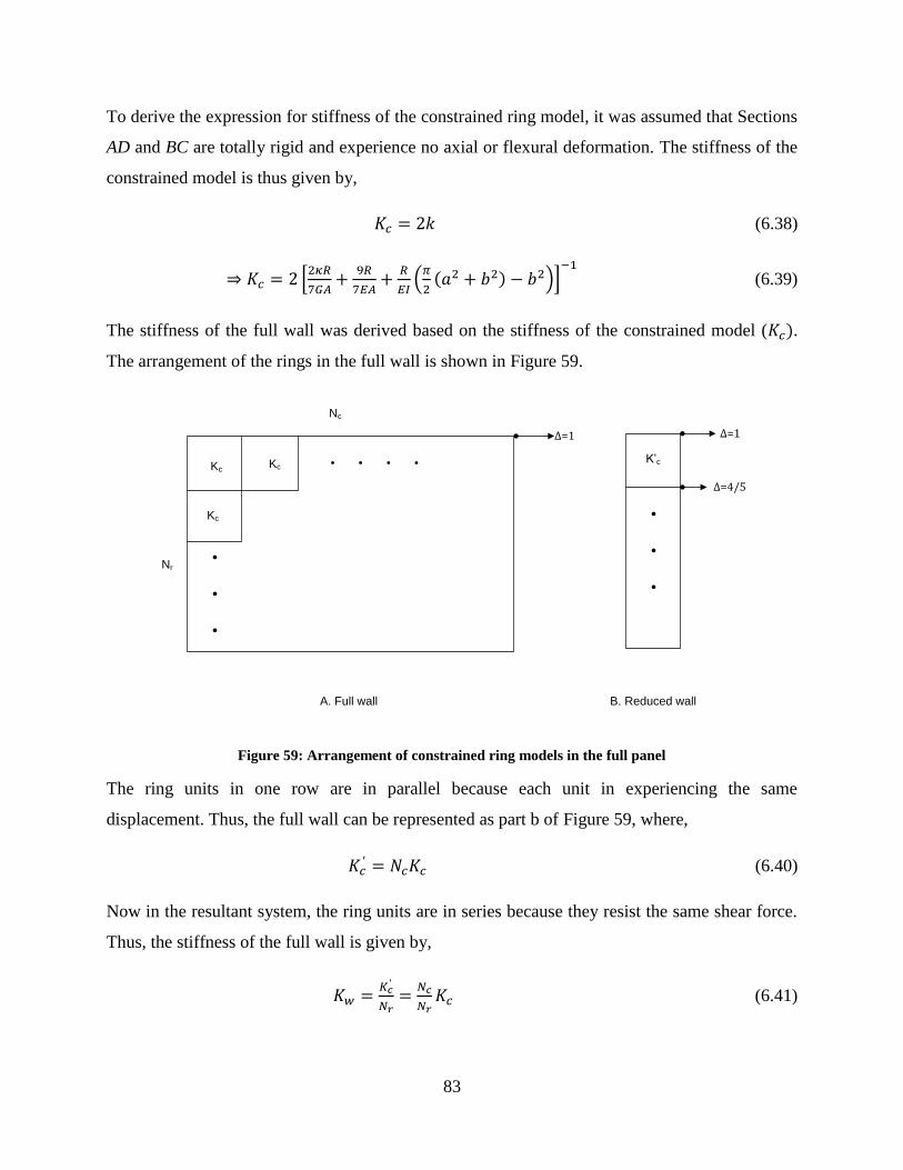
83

To derive the expression for stiffness of the constrained ring model, it was assumed that Sections

AD and BC are totally rigid and experience no axial or flexural deformation. The stiffness of the

constrained model is thus given by,

(6.38)

[

(

)]

(6.39)

The stiffness of the full wall was derived based on the stiffness of the constrained model ( .

The arrangement of the rings in the full wall is shown in Figure 59.

Δ=1

Kc

Nc

Nr

Δ=1

K’c

Δ=4/5

A. Full wall B. Reduced wall

Kc

Kc

Figure 59: Arrangement of constrained ring models in the full panel

The ring units in one row are in parallel because each unit in experiencing the same

displacement. Thus, the full wall can be represented as part b of Figure 59, where,

(6.40)

Now in the resultant system, the ring units are in series because they resist the same shear force.

Thus, the stiffness of the full wall is given by,

(6.41)

84

While deriving the equation for the stiffness using the constrained ring model, a number of

assumptions were made. First, the stiffness of the sections AD and BC and the links have been

assumed to be infinite. Also, rotation of the section AB at both the ends is assumed to be zero.

Additionally, assumptions made while deriving the stiffness for the unconstrained ring model are

also valid in this case.

It was reasoned that since the unconstrained model was restricted by fewer assumptions, it would

yield results that would approximate the mechanics of the plate more closely. Thus, the

unconstrained model was used to predict the stiffness of the BR-SPSW specimens and for

comparison of the analytical solution to the computational results obtained from the parametric

study in Chapter 8.

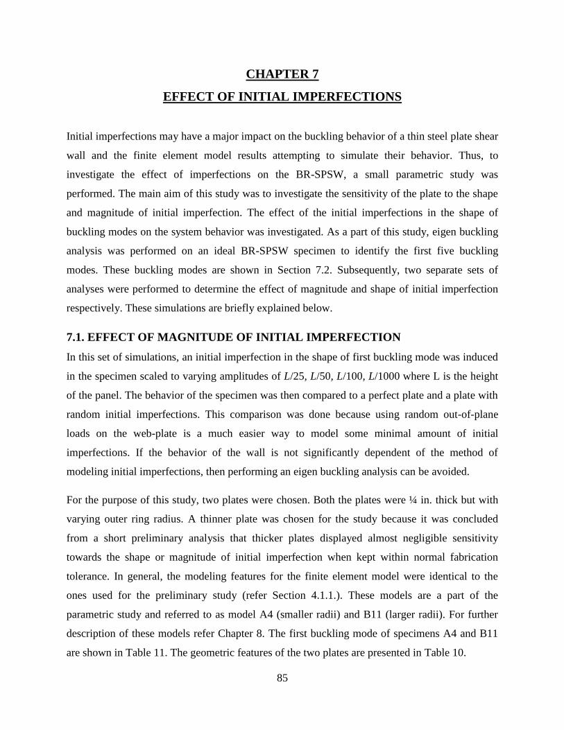
85

CHAPTER 7

EFFECT OF INITIAL IMPERFECTIONS

Initial imperfections may have a major impact on the buckling behavior of a thin steel plate shear

wall and the finite element model results attempting to simulate their behavior. Thus, to

investigate the effect of imperfections on the BR-SPSW, a small parametric study was

performed. The main aim of this study was to investigate the sensitivity of the plate to the shape

and magnitude of initial imperfection. The effect of the initial imperfections in the shape of

buckling modes on the system behavior was investigated. As a part of this study, eigen buckling

analysis was performed on an ideal BR-SPSW specimen to identify the first five buckling

modes. These buckling modes are shown in Section 7.2. Subsequently, two separate sets of

analyses were performed to determine the effect of magnitude and shape of initial imperfection

respectively. These simulations are briefly explained below.

7.1. EFFECT OF MAGNITUDE OF INITIAL IMPERFECTION

In this set of simulations, an initial imperfection in the shape of first buckling mode was induced

in the specimen scaled to varying amplitudes of L/25, L/50, L/100, L/1000 where L is the height

of the panel. The behavior of the specimen was then compared to a perfect plate and a plate with

random initial imperfections. This comparison was done because using random out-of-plane

loads on the web-plate is a much easier way to model some minimal amount of initial

imperfections. If the behavior of the wall is not significantly dependent of the method of

modeling initial imperfections, then performing an eigen buckling analysis can be avoided.

For the purpose of this study, two plates were chosen. Both the plates were ¼ in. thick but with

varying outer ring radius. A thinner plate was chosen for the study because it was concluded

from a short preliminary analysis that thicker plates displayed almost negligible sensitivity

towards the shape or magnitude of initial imperfection when kept within normal fabrication

tolerance. In general, the modeling features for the finite element model were identical to the

ones used for the preliminary study (refer Section 4.1.1.). These models are a part of the

parametric study and referred to as model A4 (smaller radii) and B11 (larger radii). For further

description of these models refer Chapter 8. The first buckling mode of specimens A4 and B11

are shown in Table 11. The geometric features of the two plates are presented in Table 10.

86

Table 10: Geometric features of A4 and B11

t (in.) Ro (in.) Ro/wc Ro/wl

A4 0.25 10 3.33 2

B11 0.25 24 3.33 2

The pushover behavior for models A4 and B11 with varying levels of initial imperfection is

shown in Figure 60 and Figure 61. From the figure it was concluded that as long as the

imperfections are included in the model and are less that L/100, the effect of the magnitude of

imperfection is small and can be neglected. For imperfections larger than L/100, the stiffness of

the panel reduces. For example, an imperfection of L/50 resulted in the reduction of the initial

stiffness by 30% for A4 and 43% for B11. In most cases higher imperfections also led to model

instability. Thus it seems reasonable to limit the initial imperfections of the BR-SPSW to L/100

for practical purposes (about 1.44 inches for this plate).

Figure 60: Effect of the magnitude of initial imperfections for plate A4

0

20

40

60

80

100

120

140

0 0.5 1 1.5 2 2.5 3 3.5 4 4.5

La

tera

l L

oa

d (

kip

s)

Lateral Displacement (in.)

Perfect geometry

Random imperfections

Imperfection L/1000

Imperfection L/100

Imperfection L/50

Imperfection L/25

87

Figure 61: Effect of initial imperfection for plate B11

It was also concluded that using random imperfections for modeling the plates is acceptable

since there was only a small difference in the capacity and stiffness of the plates as compared to

the models with initial imperfections in the shape of the first eigen-mode. Another point that

should be noted here is that large initial imperfections result in reduced strength and stiffness,

especially in model B11 which had larger radii rings. Thus, it is very important to make initial

imperfections in a model to simulate its actual behavior.

7.2. EFFECT OF THE SHAPE OF INITIAL IMPERFECTION

In this set of tests, initial imperfection in the shape of first five eigen buckling modes was used

for both plates A4 and B11. These modes are shown in Table 11. The magnitude of the

imperfection was scaled to L/100 for each case. The results were then compared to the behavior

of the plate with random imperfections. Figure 62 and Figure 63 shows the effect of the shape of

initial imperfection on the plate behavior. The mode shape clearly does not have major effect on

the stiffness and strength of the plate.

The final conclusion that was drawn from this chapter was that the use of random out-of-plane

imperfections to simulate initial imperfections is acceptable. Also, it saves computational time

0

20

40

60

80

100

120

140

0 0.5 1 1.5 2 2.5 3 3.5 4 4.5

La

tera

l L

oa

d (k

ips)


Perfect geometry

Random

Imperfection L/1000

Imperfection L/100

Imperfection L/50

Imperfection L/25

88

and effort that would be required to perform eigen buckling analysis for each plate before

running the main analysis.

Table 11: Table showing the eigen buckling modes of specimen A4 and B11

Specimen A4

Specimen A4

Specimen B11

Specimen B11

Mode

1

Mode

2

89

Mode

3

Mode

4

Mode

5

90

Figure 62: Effect of shape of initial imperfection on plate A4

Figure 63: effect of shape of initial imperfection on plate B11

0

20

40

60

80

100

120

0 0.5 1 1.5 2 2.5 3

La

tera

l L

oa

d (

kip

s)



Mode 1

Mode 2

Mode 3

Mode 4

Mode 5

0

10

20

30

40

50

60

70

80

0 0.5 1 1.5 2 2.5 3

La

tera

l L

oa

d (

kip

s)



Mode 1

Mode 2

Mode 3

Mode 4

91

CHAPTER 8

PARAMETERIC STUDY

The preliminary analyses presented in Chapter 4 were done to validate the idea behind the BR-

SPSW. The study showed that this proposed alternative to a typical shear wall reduced bucking,

exhibited higher resistance to lateral loading during load reversals, and produced much less

pinching of the hysteresis loops. Moreover, the system works well without moment connections

(i.e. has sufficient stiffness, energy dissipation, and resists force during load reversals).

To build on the preliminary work presented in previous sections, there was a need to perform

more rigorous and methodical computational study of the full-size panel with varying parameters

to better understand the behavior of this system. The parametric computational study was

performed using ABAQUS (Version 6.11 Documentation) as the main tool. 2D modeling with

shells elements was used to model the plate. Geometric non-linearities were included to capture

of the web plate. Boundary elements were modeled near rigid to isolate the behavior of the web

plate. All the other modeling parameters were identical to the preliminary studies presented in

Chapter 4. The loading protocol was however changed to a more standard protocol used for

beam-to-column moment connections. The protocol was adopted from AISC seismic provisions

(Appendix S6.2) but was modified such that only one cycle per story drift level was used as

shown in Figure 64.

Figure 64: Loading protocol used for the parametric study

-5

-4

-3

-2

-1

0

1

2

3

4

5

Dri

ft %

92

For the parametric study, the boundary elements (beam and columns) are assumed to be perfectly

rigid so as to isolate the behavior of the panel. All the output data from ABAQUS was recorded

at the middle layer of the shell elements. This was done to get axial stresses only and to avoid

getting the high bending stresses associated with out of plane buckling.

The most critical parameters identified for the computational study, the range in which they are

varied and related issues are discussed in the next section.

8.1. INPUT PARAMETERS

8.1.1. Thickness of steel plate used (t)

The web plate thicknesses to be used in the study are: 5/8 inches, 1/2 inches, 5/16 inches and 1/4

inches. These values were chosen for the steel plates so they can be used in large range of stories

with varying load demand. The initial capacity prediction shows that using these thicknesses can

result in strength in the range 50-550 kips. These values can be further increased or decreased by

changing other dimensional parameters of the panel.

8.1.2. Outer radius of the rings (Ro)

The radius of the rings has been varied in the range: 8 inches, 10 inches, 16 inches and 24 inches.

The lower bound of this range was chosen keeping in mind the fact the decreasing the diameter

of the rings increases the cutting length exponentially, thus increasing the cutting cost. The upper

bound of the range was chosen as 24 inches to further explore the design space to figure out what

combinations of design parameters result in local lateral torsional buckling in the rings.

8.1.3. Width of the rings (Wc)

The width of the rings has been varied in the form of variation in the Ro/wc ratio. This ratio is the

slenderness ratio of the ring and is expected that it may influence the buckling behavior of the

full wall. The ratio chosen for this ratio for the study are: 2, 2.5 and 3.33 and 5.These values

were chosen keeping in mind two important facts. First, very wide rings may not yield easily and

thus, reducing the dissipation energy. Second, a very narrow ring may experience local lateral

torsional buckling, both of which can have adverse effects on the performance of the wall.

8.1.4. Width of the connecting link (Wl)

This parameter is expected to affect the amount of inelastic axial deformations of the link thus

contributing to the amount of lag and pinching of the hysteretic behavior. Again, the parameter

here has been varied in the form of Ro/wlratio. The lower bound for the parameter was set

93

keeping in mind the fact that if the connecting link is too narrow, it will yield, causing an adverse

effect on the wall behavior.

Apart from the independent variables mentioned above, a few dependent and dimensionless

variables were studied to better understand the system behavior. Ro/t and wc/t also referred in this

text as the ring slenderness ratio were used to understand the local buckling of the rings which

have a major impact on the overall energy dissipation of BR-SPSW.

8.2. OUTPUT PARAMETERS

To thoroughly study the behavior of the BR-SPSW a comprehensive list of output parameters

was prepared as shown below.

Strength of the shear wall system

Stiffness of the shear wall system

Yield drift % of the shear wall system

Total energy dissipation

Energy dissipation ratio

Buckling Ratio

Length of the cut

Openness of the wall

Peak strength

Weight ratio

These output parameters were recorded for each specimen of the parametric study. This section

briefly describes each of these parameters and the methods used to record them.

8.2.1. Strength, stiffness and yield drift

Strength, stiffness and the yield drift of a shear wall system were recorded by subjecting every

specimen to a monotonic loading. The force-displacement plot was then generated as shown in

Figure 65. For stiffness, the initial slope of the curve taking the origin (0,0) and the point on the

curve which corresponds to the half of the maximum strength achieved (point-b) was recorded.

Another line was constructed taking the points corresponding to 0.75% and 1% drift on the

force-displacement plot. The intersection point of both the lines (point-a) was noted. The x-

94

coordinate of point was recorded as the strength of the shear panel and the y-coordinate as the

yield drift. Similar plots showing the calculation of strength for all the specimens are compiled as

a part of Appendix D. Each curve was examined individually to ensure that this method

produced seemingly reasonable results.

Figure 65: Strength, Stiffness and Yield Drift calculation from force-displacement plot

8.2.2. Total energy dissipation

Energy dissipation in a BR-SPSW takes places due to the yielding of the ring-link system. The

efficiency of this unique geometrical feature would therefore be reflected in the total dissipated

energy. This output parameter was recorded by taking the total area under the last hysteresis

loop. The hysteresis curve for all the specimens is recorded in Appendix B.

8.2.3. Energy Dissipation Ratio

Energy dissipation ratio is a measure of how close a specimen is to an ideal specimen which

displays full hysteretic behavior with no pinching. It is the ratio of the actual energy dissipated

by a specimen to the ideal energy dissipated, if there were not strength degradation or pinching.

Thus a higher energy dissipation ratio would indicate relatively higher energy dissipation.

95

To record this ratio, a parallelogram was constructed around the last cycle of a hysteresis curve

as shown in Figure 66. The area under the dashed parallelogram represents the energy dissipated

by an ideal specimen exhibiting full hysteretic behavior. The energy dissipation ratio is

calculated as the ratio of the area of the last cycle of the hysteresis curve to the area under the

parallelogram. To construct the parallelogram, the slopes of the adjacent edges of the

parallelogram were first determined. One of the slopes was taken as the slope of the hysteresis

curve in the last cycle right after it attains its peak strength (in the last cycle). The second slope

was slope of the hysteresis curve right before it achieves its global peak strength. The plots for

all the specimens showing the calculation of the energy dissipation ratio are attached in

Appendix C.

Figure 66: Plot showing the method for calculating the energy dissipation ratio

8.2.4 Buckling Ratio

This output parameter indicates the relative percentage of global tension buckling and lateral

torsional bucking of the rings. A higher ratio implies relatively higher percentage of global

tension field buckling. Note that this output parameter is important because the type of buckling

modes (global tension field buckling or lateral torsional bucking of the rings) has an impact on

the total energy dissipation of the shear wall. This will be elaborated in a Section 8.4.2.

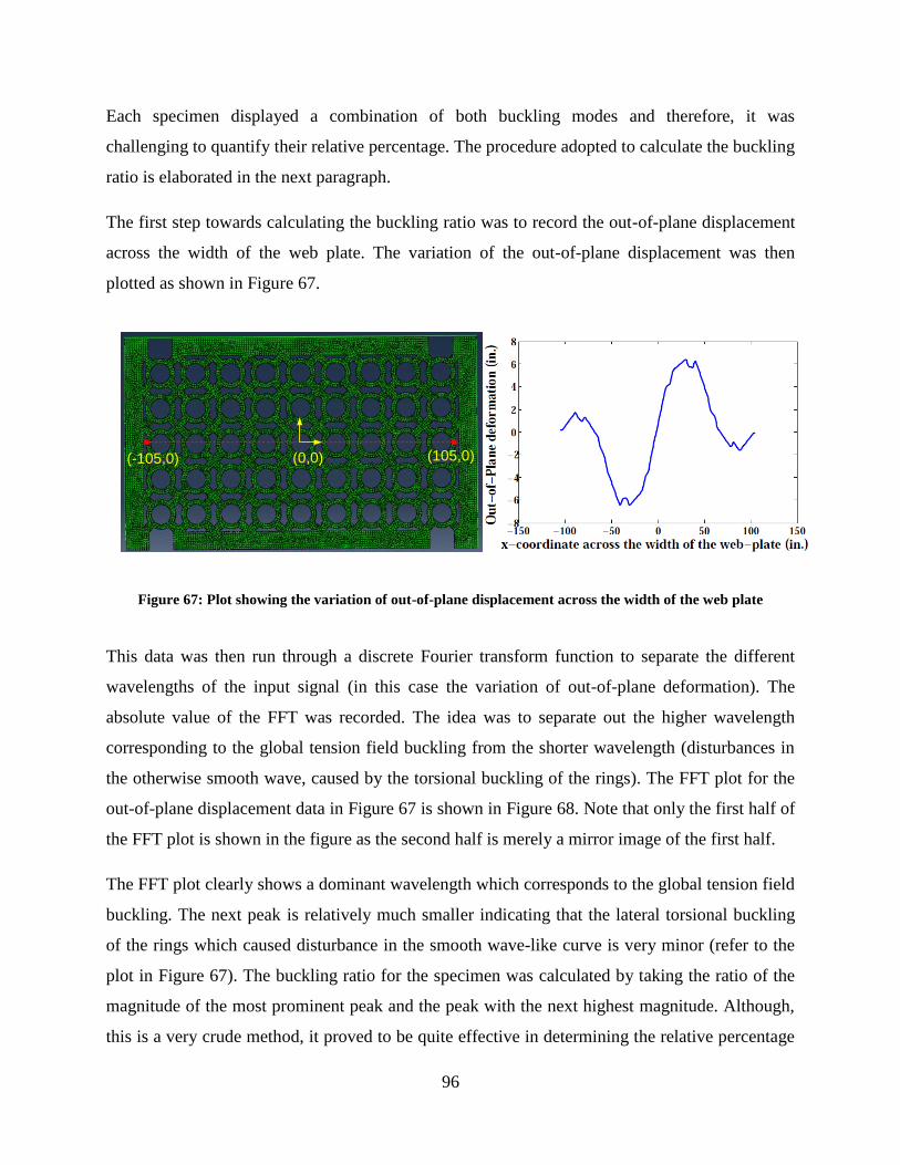
96

Each specimen displayed a combination of both buckling modes and therefore, it was

challenging to quantify their relative percentage. The procedure adopted to calculate the buckling

ratio is elaborated in the next paragraph.

The first step towards calculating the buckling ratio was to record the out-of-plane displacement

across the width of the web plate. The variation of the out-of-plane displacement was then

plotted as shown in Figure 67.

(0,0)(-105,0) (105,0)

Figure 67: Plot showing the variation of out-of-plane displacement across the width of the web plate

This data was then run through a discrete Fourier transform function to separate the different

wavelengths of the input signal (in this case the variation of out-of-plane deformation). The

absolute value of the FFT was recorded. The idea was to separate out the higher wavelength

corresponding to the global tension field buckling from the shorter wavelength (disturbances in

the otherwise smooth wave, caused by the torsional buckling of the rings). The FFT plot for the

out-of-plane displacement data in Figure 67 is shown in Figure 68. Note that only the first half of

the FFT plot is shown in the figure as the second half is merely a mirror image of the first half.

The FFT plot clearly shows a dominant wavelength which corresponds to the global tension field

buckling. The next peak is relatively much smaller indicating that the lateral torsional buckling

of the rings which caused disturbance in the smooth wave-like curve is very minor (refer to the

plot in Figure 67). The buckling ratio for the specimen was calculated by taking the ratio of the

magnitude of the most prominent peak and the peak with the next highest magnitude. Although,

this is a very crude method, it proved to be quite effective in determining the relative percentage

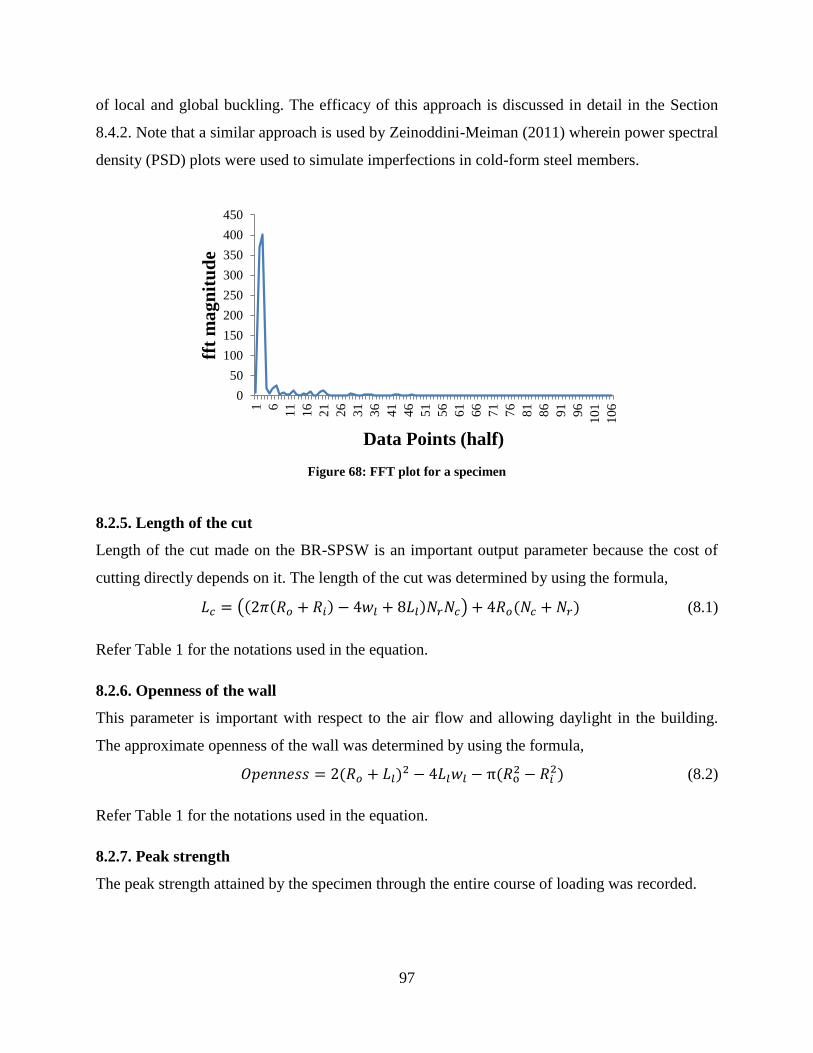
97

of local and global buckling. The efficacy of this approach is discussed in detail in the Section

8.4.2. Note that a similar approach is used by Zeinoddini-Meiman (2011) wherein power spectral

density (PSD) plots were used to simulate imperfections in cold-form steel members.

Figure 68: FFT plot for a specimen

8.2.5. Length of the cut

Length of the cut made on the BR-SPSW is an important output parameter because the cost of

cutting directly depends on it. The length of the cut was determined by using the formula,

( ) (8.1)

Refer Table 1 for the notations used in the equation.

8.2.6. Openness of the wall

This parameter is important with respect to the air flow and allowing daylight in the building.

The approximate openness of the wall was determined by using the formula,

(8.2)

Refer Table 1 for the notations used in the equation.

8.2.7. Peak strength

The peak strength attained by the specimen through the entire course of loading was recorded.

0

50

100

150

200

250

300

350

400

450

1 6

11

16

21

26

31

36

41

46

51

56

61

66

71

76

81

86

91

96

101

106

fft

ma

gn

itu

de

Data Points (half)

98

8.2.8. Weight ratio

The weight ratio was defined as the ratio of the weight of BR-SPSW (considering the cut-out

pattern) specimen to the weight of a solid panel having the same strength as the BR-SPSW

specimen.

The expression used for the strength of the solid panel is given by (Berman and Bruneau, 2007),

(8.3)

where, t is the thickness of the plate, W is the width of the plate and is the angle of inclination

of tension field (taken as 40ᵒ in this report). For calculating the strength of BR-SPSW, equation

5.70 was used.

8.3. TEST SETS

A detailed summary of all the analyses to be performed as a part of the computational study is

presented in

Table 12-15. Each series of tests is designed to study the influence of a specific parameter on the

overall behavior of the panel. Refer to Section 8.1 for the definition of the input parameters used

in the parametric study.

Note the staggered configuration, which was analyzed as a part of the preliminary study was

excluded from the main parametric study. The reason behind this decision was the difficulty in

the ring arrangement for a given web-plate dimension.

Meshing the models with appropriate mesh size is quite essential for obtaining accurate results

from FE analysis. However, too much mesh refinement is computationally expensive. Thus,

before starting the parametric study, two mesh sizes (seed size 0.75 and 1.5) were used for

specimen A1. Note that an element seed size of 1.5 was used for preliminary study.

It was observed that the difference in the major output parameters (strength, stiffness, yield drift

%, energy dissipation) for the two models was less than 9%. The use of element seed size of 1.5

was thus justified and was used for the parametric study.

99

Table 12: Table showing the tests done as a part of SERIES A of the parametric study

SERIES A: To determine the influence of thickness(tw)

tw Ro Ro/wc wc Ro/wL wL Ro/tw

A1 5/8'' 10'' 3.33 3'' 2 5'' 16

A2 1/2'' 10'' 3.33 3'' 2 5'' 20

A3 5/16'' 10'' 3.33 3'' 2 5'' 32

A4 1/4'' 10'' 3.33 3'' 2 5'' 40

Table 13: Table showing the tests done as a part of SERIES B of the parametric study

SERIES B: To determine the influence of outer radius Ro


B1 1/2'' 24'' 3.33 7.2'' 2 12'' 48

B2 5/8'' 16'' 3.33 4.8'' 2 8'' 25.6

B3 5/16'' 8'' 3.33 2.4'' 2 4'' 25.6

B4 5/8'' 24'' 3.33 7.2'' 2 12'' 38.4

B5 1/2 '' 16'' 3.33 4.8'' 2 8'' 32

B6 1/4'' 16'' 3.33 4.8'' 2 8'' 64

B7 5/8'' 8'' 3.33 2.4'' 2 4'' 12.8

B8 1/4'' 8'' 3.33 2.4'' 2 4'' 32

B9 1/2'' 8'' 3.33 2.4'' 2 4'' 16

B10 5/16'' 16'' 3.33 4.8'' 2 8'' 51.2

B11 1/4'' 24'' 3.33 7.2'' 2 12'' 96

B12 5/16'' 24'' 3.33 7.2'' 2 12'' 76.8

100

Table 14: Table showing the tests done as a part of SERIES C of the parametric study

SERIES C :To determine the influence of Ro/wc and Ro/wl ratio


C1 1/2'' 10'' 5 2'' 2 5'' 20

C2 5/8'' 16'' 2.5 6.4'' 2 8'' 16

C3 5/16'' 8'' 5 1.6'' 2 4'' 32

C4 5/8'' 10'' 2.5 4'' 2 5'' 16

C5 1/2 '' 16'' 5 3.2'' 2 8'' 20

C7 1/2'' 10'' 2.5 4'' 2 5'' 20

C8 5/8'' 8'' 2.5 3.2'' 2 4'' 12.8

C9 1/2'' 8'' 2.5 3.2'' 2 4'' 16

C10 5/16'' 10'' 2.5 4'' 2 5'' 32

C11 5/8'' 10'' 5 2'' 2 5'' 16

C12 5/16'' 10'' 2 5'' 2 5'' 32

C13 1/2'' 10'' 2 5'' 2 5'' 20

C14 5/8'' 10'' 2 5'' 2 5'' 16

C15 5/8'' 10'' 3.33 3'' 1.5 6.667'' 16

C16 1/2'' 10'' 3.33 3'' 1.5 6.667'' 20

C17 5/16'' 10'' 3.33 3'' 1.5 6.667'' 32

C18 5/8'' 10'' 3.33 3'' 2.5 4'' 16

C19 1/2'' 10'' 3.33 3'' 2.5 4'' 20

C20 5/16'' 10'' 3.33 3'' 2.5 4'' 32

C21 5/8'' 10'' 3.33 3'' 3 3.33'' 16

C22 1/2'' 10'' 3.33 3'' 3 3.33'' 20

C23 5/16'' 10'' 3.33 3'' 3 3.33'' 32

101

Table 15: Table showing the tests done as a part of SERIES D of the parametric study

SERIES D: To determine the influence of Ro/wl and Ro/wc ratio


D1 5/8'' 10'' 3.33 3'' 3 3.33'' 16

D2 5/8'' 16'' 2.5 6.4'' 1.5 10.67'' 16

D3 1/2'' 10'' 5 2'' 3 3.33'' 20

D4 5/16'' 8'' 2.5 3.2 3 2.67'' 25.6

D5 1/2'' 8'' 3.33 2.4'' 1.5 5.33'' 20

D6 1/2'' 24'' 3.33 7.2'' 1.5 16'' 20

D7 1/2'' 8'' 2.5 3.2 3 2.67'' 16

D8 1/2'' 10'' 2.5 4'' 3 3.33'' 20

D9 1/2'' 10'' 2.5 4'' 2.5 4'' 20

D10 1/2'' 8'' 2.5 3.2'' 2.5 3.2 16

D11 1/2'' 16'' 2.5 6.4'' 2 8'' 32

D12 1/2'' 16'' 2.5 6.4'' 2.5 6.4'' 32

D13 1/2'' 16'' 2.5 6.4'' 3 5.33'' 32

8.4. RESULTS AND DISCUSSION

This section discusses the results of the parametric study. Conclusions related to the behavior of

BR-SPSW have been drawn and recommendations have been made for optimum design.

8.4.1. Hysteretic behavior

As previously mentioned, hysteresis plots for each specimen in the parametric study was

generated. The hysteresis plot reflects the behavior of a specimen under cyclic loading,

specifically its energy dissipation capability. As highlighted previously, the main purpose of the

parametric study was to investigate the sensitivity of the system behavior on the input

parameters. The hysteresis plot of all the test specimens was keenly observed to derive

appropriate conclusion.

One of the major input parameter for the parametric study was the thickness of the steel plate

used. It was observed as the plate thickness decreases, the energy dissipation capacity of the

specimen decreases as is clear from the shrinking area under the curve in Figure 69. This

observation can be attributed to the fact that thinner plates buckle faster and hence experience

102

significant strength and stiffness degradation. For example, specimen A4 with thinnest web plate

suffered a reduction in stiffness of about 66% in the last cycle as compared to the first cycle.

This decrease was comparatively less (52%) for specimen A2. A much detailed and quantitative

analysis of the dependence of system behavior on the thickness of the web plate is presented in

Section 8.4.3.

(t=1/2’’)

(t=1/4’’)

(t=5/16'’)(t=1/2’’)

Figure 69: Figure showing the dependence of hysteretic behavior on thickness for 10’’ outer ring radius

Next, the dependence of the hysteretic behavior on the ring radius was investigated. It was

observed that increase in the outer ring radius resulted in lower energy dissipation as shown in

Figure 70. The FE analysis results showed that specimens with larger ring radius (B5 and B1)

exhibited severe lateral torsional buckling of the rings as opposed to their smaller radii

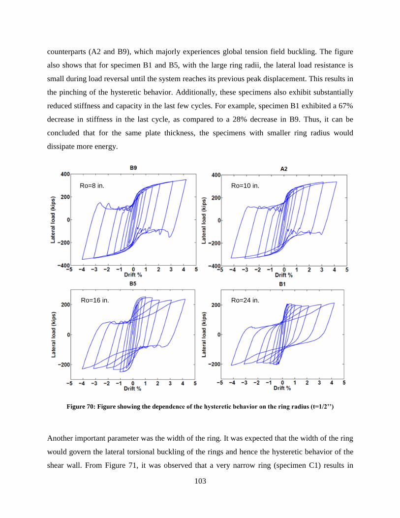
103

counterparts (A2 and B9), which majorly experiences global tension field buckling. The figure

also shows that for specimen B1 and B5, with the large ring radii, the lateral load resistance is

small during load reversal until the system reaches its previous peak displacement. This results in

the pinching of the hysteretic behavior. Additionally, these specimens also exhibit substantially

reduced stiffness and capacity in the last few cycles. For example, specimen B1 exhibited a 67%

decrease in stiffness in the last cycle, as compared to a 28% decrease in B9. Thus, it can be

concluded that for the same plate thickness, the specimens with smaller ring radius would

dissipate more energy.

Ro=8 in. Ro=10 in.

Ro=16 in. Ro=24 in.

Figure 70: Figure showing the dependence of the hysteretic behavior on the ring radius (t=1/2’’)

Another important parameter was the width of the ring. It was expected that the width of the ring

would govern the lateral torsional buckling of the rings and hence the hysteretic behavior of the

shear wall. From Figure 71, it was observed that a very narrow ring (specimen C1) results in

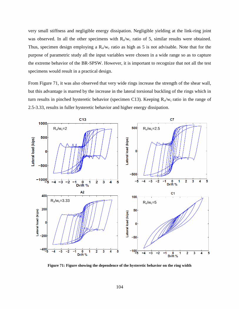
104

very small stiffness and negligible energy dissipation. Negligible yielding at the link-ring joint

was observed. In all the other specimens with Ro/wc ratio of 5, similar results were obtained.

Thus, specimen design employing a Ro/wc ratio as high as 5 is not advisable. Note that for the

purpose of parametric study all the input variables were chosen in a wide range so as to capture

the extreme behavior of the BR-SPSW. However, it is important to recognize that not all the test

specimens would result in a practical design.

From Figure 71, it was also observed that very wide rings increase the strength of the shear wall,

but this advantage is marred by the increase in the lateral torsional buckling of the rings which in

turn results in pinched hysteretic behavior (specimen C13). Keeping Ro/wc ratio in the range of

2.5-3.33, results in fuller hysteretic behavior and higher energy dissipation.

Ro/wc=2 Ro/wc=2.5

Ro/wc=3.33 Ro/wc=5

Figure 71: Figure showing the dependence of the hysteretic behavior on the ring width

105

The dependence of other input parameters on the system response will be further investigated in

Section 8.4.3. with the help of trend plots.

8.4.2. Buckling ratio

As mentioned in Section 8.2.4, the buckling ratio of each specimen was derived from the discrete

Fourier transform of the out-of-plane deformation data. The main goal of this exercise was to

quantify the relative percentage of local torsional buckling and global tension field buckling in a

BR-SPSW. The next paragraph presents the effectiveness of the method in decomposing the

buckling modes.

Using the procedure mentioned in Section 8.2.4, the variation of out-of-plane deformation for

Specimen A1 and A4 was generated as shown in Figure 72. The screen shot of the specimens

show the out-of-plane deformation (U3) wherein blue and red color represents its maximum

value in the positive and negative direction. Figure 72 shows the smooth wave-like variation of

out-of-plane deformation in specimen A1 which is a result of global tension field buckling. In

specimen A4, however, this variation sees minor disturbances as a result of lateral torsional

buckling of the ring.

This difference in the variation of out-of-plane deformation is reflected in the FFT plots

generated for the two sets of data as shown in Figure 73. The smooth variation with little or no

disturbance (specimen A1) translates to Fourier transform with a prominent wavelength of high

magnitude. Major disturbances in this curve would result in more than one prominent peak in the

FFT plots corresponding to the major wavelengths forming the curve. The ratio of the

magnitudes of the first peak and the second peak is thus a crude, albeit effective way of

measuring the deviation from the smooth wave-like variation of out-of-plane deformation. This

ratio, referred to as the buckling ratio in this text, is thus indicative of the relative percentage of

the global and local buckling in BR-SPSW.

As indicated in the Figure 73, the buckling ratio for specimen A1 is much higher (33.3) as

compared to its thinner counterpart A4 with a buckling ratio of 8.5. This is expected because the

ring units in A4 have a much higher Ro/t (ring slenderness ratio). This results in local torsional

buckling of the rings. Another important observation that can be made from Figure 73 is that the

106

most prominent wavelength obtained from the FFT plots is almost of the order of the width of

the plate. Similarly, the second prominent wavelength is of the order of the ring diameter.

The dependence of the buckling ratio on other input parameters has been discussed in detail in

the Section 8.4.3.

x

y

Specimen A1

107

x

y

Specimen A4

Figure 72: Variation of out-of-plane deformation across the width of the web-plate

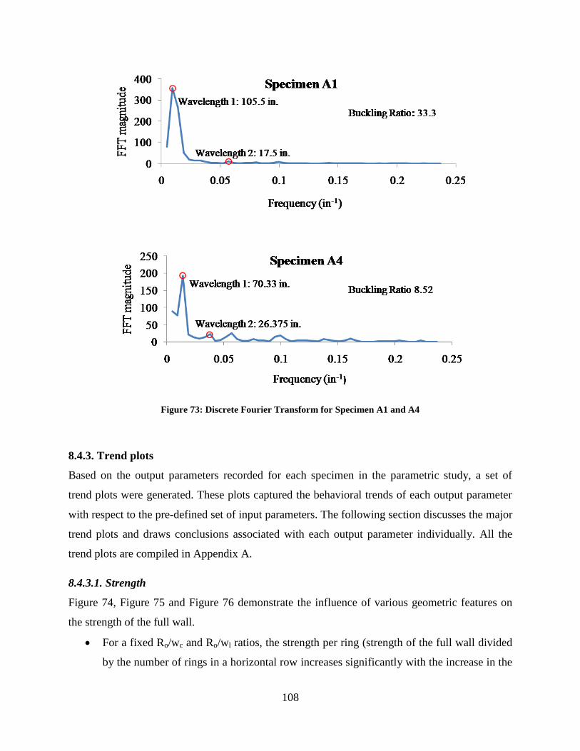
108

Figure 73: Discrete Fourier Transform for Specimen A1 and A4

8.4.3. Trend plots

Based on the output parameters recorded for each specimen in the parametric study, a set of

trend plots were generated. These plots captured the behavioral trends of each output parameter

with respect to the pre-defined set of input parameters. The following section discusses the major

trend plots and draws conclusions associated with each output parameter individually. All the

trend plots are compiled in Appendix A.

8.4.3.1. Strength

Figure 74, Figure 75 and Figure 76 demonstrate the influence of various geometric features on

the strength of the full wall.

For a fixed Ro/wc and Ro/wl ratios, the strength per ring (strength of the full wall divided

by the number of rings in a horizontal row increases significantly with the increase in the

109

plate thickness. This effect slowly decreases as the radius of the ring decreases. This is

evident from Figure 74, where a 5/16th

inch increase in the plate thickness (from 5/16th

in.

to 5/8th

in.), results in 175% increases in the strength/ring for a 24 inch radius shear plate.

This increase is, however relatively small for an 8 inch radius (110%).

For a given ring radius and link width, it was concluded that both Ro/t and Ro/wc ratios

affect the strength/ ring significantly. From Figure 75, it was concluded that increase in

both Ro/t and Ro/wc ratios have depreciating effect on the strength of a unit ring. Since the

radius is fixed here, the decreasing strength of the ring with the Ro/wc merely suggest that

decreasing the width of the ring will result in lower strength/unit ring

For a fixed ring radius and ring width, the strength/ring slightly decreases with the width

of the link. This is due to the slight shift in the position of the plastic hinges. This

dependence of the width of the link on strength is reflected in Equation 5.70. This effect

is negligible as the thickness of the plate decreases. Also, comparing Figure 75 and

Figure 76 it can be concluded that as compared to the width of the link, width of the ring

has a larger influence on the ring unit strength. For example, for a Ro/t of 20, a 0.5

increase in Ro/wc results in 31% decrease in strength. A similar increase in Ro/wl, results

in only 16% decrease in strength/ring unit.

From design point of view, the trend charts presented below could act as a tool for designing

plates with desired strength. Typically, higher strength can be obtained by using thicker web

plates. While this is still true, the biggest advantage of BR-SPSW is that higher strength can still

be achieved by varying other geometric parameters. Conversely, if a thicker plate is easily

available, it can still be used in cases of lower load demands by altering other geometrical

features.

For example, as shown in Figure 74, a strength of 25 kips / ring can be achieved using Ro=24”

&t=1/4”, Ro=24” & t=0.5”, or Ro=8” & t=5/8” along with fixed values of Ro/wc=3.33 and

Ro/wl=2.0. The choice between these configurations might be based on stiffness or hysteretic

energy absorption. However, since this is stated in strength per ring, the size of the full panel

and number of rings in the full panel must also be considered.

110

Figure 74: Effect of web plate thickness and radius on strength/ring

Figure 75: Effect of Ro/wc and Ro/t ratios on strength/ring unit

Ro/wc=3.33 Ro/wl=2

Ro=10 in. Ro/wl=2

111

Figure 76: Effect of Ro/wl and Ro/t ratios on strength/ring unit

8.4.3.2. Stiffness

Figure 77, Figure 78 and Figure 79 demonstrate the influence of various geometric features on

the strength of the full wall.

For a fixed Ro/wc and Ro/wl ratios, the stiffness per ring increases linearly with the

increase in the plate thickness. As shown in Figure 77. An increase of 3/8th

inch in the

plate thickness results in about 150% increase in the stiffness/ring. For smaller radii, the

stiffness/ring does not change much with thickness.

As previously concluded in the case of strength, for a given ring radius and link width,

both Ro/t and Ro/wc ratios affect the strength/ ring significantly. From Figure 78, it was

concluded that increase in both Ro/t and Ro/wc ratios have depreciating effect on the

stiffness of a unit ring. Since the radius is fixed here, the decreasing stiffness of the ring

with the Ro/wc merely suggest that decreasing the width of the ring will result in lower

stiffness/unit ring

Ro=10 in. Ro/wc=3.33

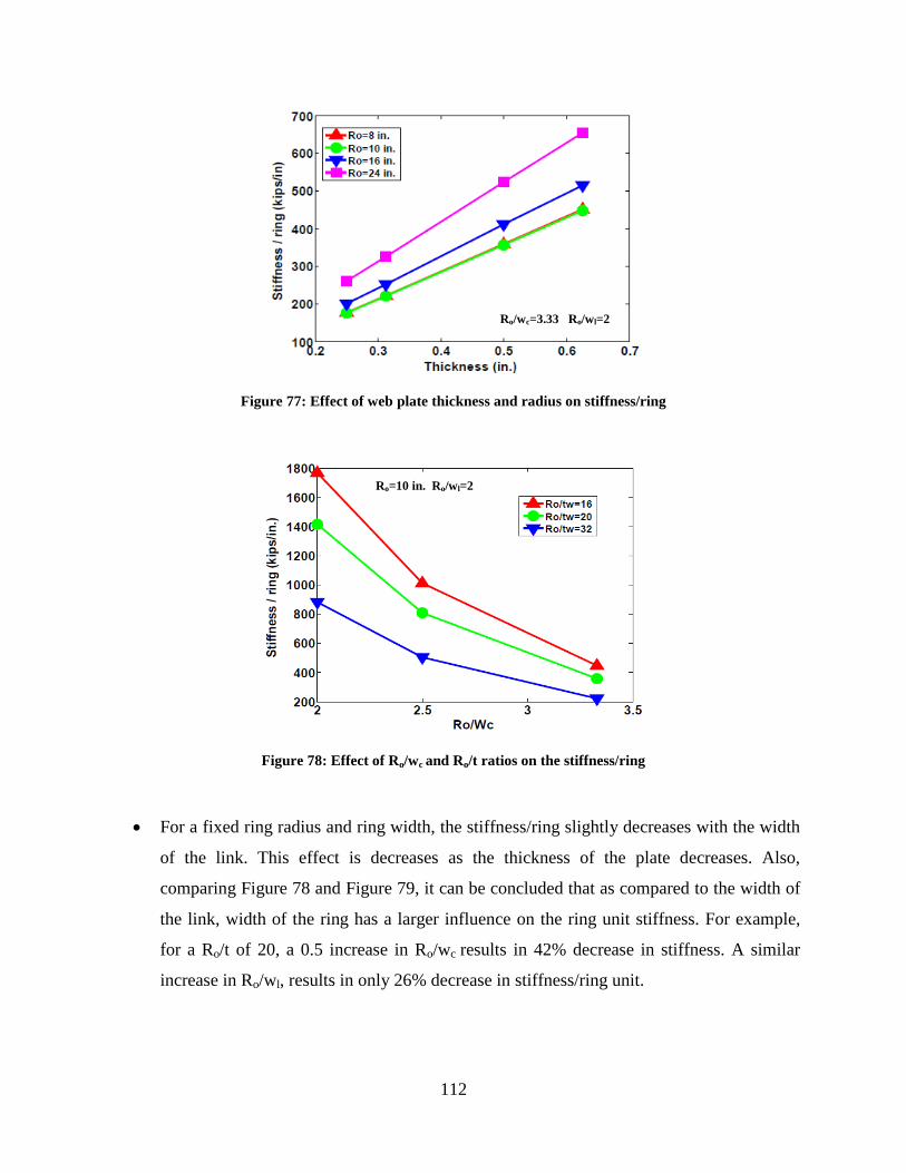
112

Figure 77: Effect of web plate thickness and radius on stiffness/ring

Figure 78: Effect of Ro/wc and Ro/t ratios on the stiffness/ring

For a fixed ring radius and ring width, the stiffness/ring slightly decreases with the width

of the link. This effect is decreases as the thickness of the plate decreases. Also,

comparing Figure 78 and Figure 79, it can be concluded that as compared to the width of

the link, width of the ring has a larger influence on the ring unit stiffness. For example,

for a Ro/t of 20, a 0.5 increase in Ro/wc results in 42% decrease in stiffness. A similar

increase in Ro/wl, results in only 26% decrease in stiffness/ring unit.

Ro/wc=3.33 Ro/wl=2

Ro=10 in. Ro/wl=2

113

Figure 79: Effect of Ro/wl and Ro/t on stiffness/ring

As observed from section 8.4.3.1 and 8.4.3.2, strength and stiffness per ring of BR-SPSW have

similar behavioral trends with respect to the major input parameters. It is therefore difficult to

separately tune strength and stiffness per ring. However, as per the analytical solutions derived

for the strength and stiffness of the full wall, it can be concluded the number of rings in BR-

SPSW does not have the same influence on the aforementioned output parameters (refer Eq. 5.70

and 6.22). Thus strength and stiffness of the full wall can be separately tuned by changing

number of rings in rows and/or columns. This can be done either by using a specific shear wall

outer dimension or by changing the length of the links.

8.4.3.3. Total energy dissipation

In this section, Figure 80, Figure 81 and Figure 83 have been used to demonstrate the

influence of various geometric features on the strength of the full wall. For fixed Ro/wc

and Ro/wl ratios, total dissipated energy increases significantly with increase in thickness.

In Figure 80, for a SPSW with a 10 inch outer radius, an increase of 3/8th

inch results in

about 350% increase in the total dissipated energy. This is increase is due to the fact that

increase in web plate thickness delays buckling and improves the hysteretic response of

the BR-SPSW. Another conclusion that can be drawn from Figure 80 is that web plates

with lower radii rings dissipate relatively more energy than the ones with larger radii.

This phenomenon is explained in subsequent sections in detail.


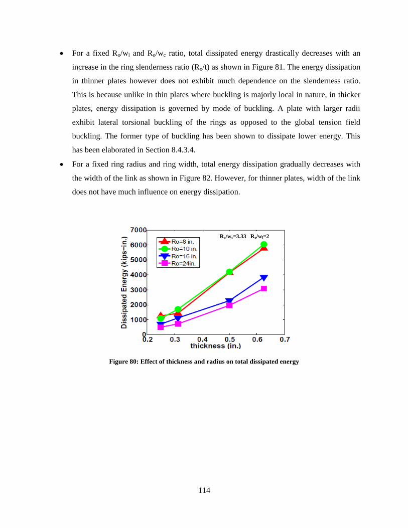
114

For a fixed Ro/wl and Ro/wc ratio, total dissipated energy drastically decreases with an

increase in the ring slenderness ratio (Ro/t) as shown in Figure 81. The energy dissipation

in thinner plates however does not exhibit much dependence on the slenderness ratio.

This is because unlike in thin plates where buckling is majorly local in nature, in thicker

plates, energy dissipation is governed by mode of buckling. A plate with larger radii

exhibit lateral torsional buckling of the rings as opposed to the global tension field

buckling. The former type of buckling has been shown to dissipate lower energy. This

has been elaborated in Section 8.4.3.4.

For a fixed ring radius and ring width, total energy dissipation gradually decreases with

the width of the link as shown in Figure 82. However, for thinner plates, width of the link

does not have much influence on energy dissipation.

Figure 80: Effect of thickness and radius on total dissipated energy

Ro/wc=3.33 Ro/wl=2

115

Figure 81: Effect of Ro/t on the total dissipated energy

Similarly, for a fixed ring radius and link width, total energy dissipation gradually

decreases with the width of the ring as shown in Figure 83. However, for thinner plates,

width of the ring does not have much influence on energy dissipation. However, as

compared to the width of the link, width of the ring has a larger influence on the total

dissipated energy. For example, for Ro/t of 16, a 0.5 increase in Ro/wc resulted in 25%

decrease in the total dissipated energy. A similar increase in Ro/wl, results in only 15%

decrease in total dissipated energy.

Ro/wc=3.33 Ro/wl=2

Figure 82: Effect of Ro/wl on total dissipated energy


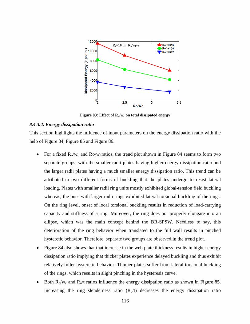
116

Figure 83: Effect of Ro/wc on total dissipated energy

8.4.3.4. Energy dissipation ratio

This section highlights the influence of input parameters on the energy dissipation ratio with the

help of Figure 84, Figure 85 and Figure 86.

For a fixed Ro/wc and Ro/wl ratios, the trend plot shown in Figure 84 seems to form two

separate groups, with the smaller radii plates having higher energy dissipation ratio and

the larger radii plates having a much smaller energy dissipation ratio. This trend can be

attributed to two different forms of buckling that the plates undergo to resist lateral

loading. Plates with smaller radii ring units mostly exhibited global-tension field buckling

whereas, the ones with larger radii rings exhibited lateral torsional buckling of the rings.

On the ring level, onset of local torsional buckling results in reduction of load-carrying

capacity and stiffness of a ring. Moreover, the ring does not properly elongate into an

ellipse, which was the main concept behind the BR-SPSW. Needless to say, this

deterioration of the ring behavior when translated to the full wall results in pinched

hysteretic behavior. Therefore, separate two groups are observed in the trend plot.

Figure 84 also shows that that increase in the web plate thickness results in higher energy

dissipation ratio implying that thicker plates experience delayed buckling and thus exhibit

relatively fuller hysteretic behavior. Thinner plates suffer from lateral torsional buckling

of the rings, which results in slight pinching in the hysteresis curve.

Both Ro/wc and Ro/t ratios influence the energy dissipation ratio as shown in Figure 85.

Increasing the ring slenderness ratio (Ro/t) decreases the energy dissipation ratio

Ro=10 in. Ro/wl=2

117

considerably. It can also be concluded from Figure 85 that increasing the width of the

ring reduces the energy dissipation ratio. This happens because a wider ring buckles in a

lateral torsional mode, which results in a much lower energy dissipation than the

specimen with narrow rings.

For a fixed ring radius and ring width, width of the link has negligible effect on the

energy dissipation ratio of the wall. This effect is clear from Figure 86. This result is

extremely important because in Section 4.1, it was conjectured that the reducing the

yielding of the link geometry result in increasing the fullness of the hysteretic behavior.

Yet Figure 86 shows that link width doesn’t have much influence on the hysteretic

behavior.

Figure 84: Effect of thickness and radius on energy dissipation ratio

Ro/wc=3.33 Ro/wl=2

118

Figure 85: Effect of Ro/wc and Ro/t on energy dissipation ratio

Figure 86: Effect of Ro/wl on energy dissipation ratio

8.4.3.5. Buckling ratio

Figure 87, Figure 88 and Figure 89 demonstrate the influence of the major input parameters on

the buckling ratio.

For a fixed Ro/wc and Ro/wl ratios, buckling ratio increases with web plate thickness.

This implies that thicker plates tend to exhibit global tension field buckling as opposed to

lateral torsional buckling of the rings which is local in nature. For larger radii plates

however, thickness has negligible influence on the buckling radii. This implies that

irrespective of the thickness, these plates suffer from lateral torsional buckling of the

rings and thus exhibit very low buckling ratio. This trend is shown in Figure 87.

Ro=10 in. Ro/wl=2


119

Figure 87: Effect of radius and thickness on buckling ratio

For a fixed Ro/wc and Ro/wl ratios, buckling ratio decreases drastically with the

slenderness ratios (wc/t, Ro/t) as shown in Figure 88 and Figure 89.

For a fixed ring radius and ring width, buckling ratio almost increases exponentially as

the width of the ring decreases implying that wider rings can easily undergo lateral

torsional buckling. This trend is shown in Figure 90.

Figure 88: Effect of wc/t on buckling ratio

Ro/wc=3.33 Ro/wl=2

Ro/wc=3.33 Ro/wl=2

120

Figure 89: Effect of Ro/t on buckling ratio

Figure 90: Effect of Ro/wc and Ro/t on buckling ratio

8.4.3.6. Length of cut

For a fixed Ro/wc and Ro/wl ratios, length of the cut exponentially decreases with an

increase in the ring radius as shown in Figure 91. Since cost of cutting is directly

proportional to the length of the cut, using a 16in. radius ring instead of 8 in. ring, for

example, would result in about 45% reduction in the cutting cost.

Ro/wc=3.33 Ro/wl=2

Ro=10 in. Ro/wl=2

121

Figure 91: Effect of ring radius on the length of cut

For a fixed ring radius and ring width, length of the cut exponentially increases as the

width of the link decreases as a shown in Figure 92. However this increase is not

substantial (a 0.5 increase in Ro/wl only increases the cutting length by 5%).

Similarly, for a fixed ring radius and link width, length of the cut exponentially increases

as the width of the ring decreases as shown in Figure 93. However this increase is not

substantial. (0.5 increase in Ro/wc ratio increases the cutting length by less than 5%).

Figure 92: Effect of Ro/wl on the length of cut

122

Figure 93: Effect of Ro/wc on the length of cut

8.4.3.7. Yield drift

For a fixed Ro/wc and Ro/wl ratios, yield drift of the shear wall increases with web plate

thickness as shown in Figure 94. For a large radius, this increase can be as much as 50%,

however, as the radius of the ring decreases, this increase is not significant (only 6% for 8

inch radius ring).

For a given radius and link width, yield drift of the shear wall does not depend

significantly on the slenderness ratio Ro/t. It, however, linearly increases as the width of

the ring decreases. This trend is shown in Figure 95.

For a fixed Ro/wc and Ro/wl ratios, yield drift drastically decreases with the slenderness

ratio wc/t and Ro/t as shown in Figure 96 and Figure 97.

123

Figure 94: Effect of thickness and radius on yield drift

Figure 95: Effect of Ro/wc and Ro/t on yield drift

Figure 96: Effect of wc/t on yield drift

Ro/wc=3.33 Ro/wl=2

Ro=10 in. Ro/wl=2

Ro/wc=3.33 Ro/wl=2

124

Figure 97: Effect of Ro/t on yield drift

The output parameters recorded for each specimen is summarized in Table 16. Note that some

tests were deleted from the test matrix because the ABAQUS analysis for those specimens got

aborted due to convergence issues.

Table 16: Output parameters for the test specimens of SERIES A

Strength

(kips)

Peak

Strength

(kips)

Stiffness

(kips/in)

Yield

Drift (%)

Length

of cut

(inches)

Open-

ness of

the wall

(in2)

Energy

dissipation

(kips-in)

Energy

Dissipation

Ratio

Weight

Ratio

Buckling

ratio

A1 280 465 582 0.32 6204 13327 6047 0.76 6.76 33.3

A2 226 339 464 0.319 6204 13327 4190 0.71 6.8 22.76

A3 136 166 288 0.3 6204 13327 1697 0.55 7.19 15.85

A4 110 119 230 0.295 6204 13327 1073 0.49 7.49 8.53

Ro/wc=3.33 Ro/wl=2

125

Table 17: Output parameters for the test specimens of SERIES B

Strength

(kips)

Peak

Strength

(kips)

Stiffness

(kips/in)

Yield

Drift (%)

Length

of cut

(inches)

Open-

ness of

the wall

(in2)

Energy

dissipation

(kips-in)

Energy

Dissipation

Ratio

Weight

Ratio

Buckling

ratio

B1 200 213 524 0.249 2464 13009 1960 0.48 7.849 4.68

B2 265 353 601 0.291 3818 14455 3835 0.57 6.81 5.93

B3 127 173 278 0.29 7124 14455 1420 0.62 7.315 33.49

B4 260 290 654 0.27 2464 13009 3070 0.54 7.18 3.78

B5 213 253 480 0.291 3818 14455 2268 0.46 6.82 4.55

B6 107 94 235 0.228 3818 14455 704 0.41 6.37 4.51

B7 267 465 565 0.313 7029 14647 5765 0.69 6.73 59.15

B8 100 123 222 0.294 7029 14647 1243 0.54 7.24 11.55

B9 213 350 450 0.303 7029 14647 4154 0.72 6.94 54.7

B10 123 126.41 294 0.275 3818 14455 1106 0.46 7.351 3.85

B11 68 87.78 261 0.177 2464 13009 493 0.37 11.06 5.36

B12 98 117 326 0.208 2464 13009 711 0.4 9.406 3.4

Table 18: Output parameters for the test specimens of SERIES C

Strength

(kips)

Peak

Strength

(kips)

Stiffness

(kips/in)

Yield

Drift (%)

Length

of cut

(inches)

Open-

ness of

the wall

(in2)

Energy

dissipation

(kips-in)

Energy

Dissipation

Ratio

Weight

Ratio

Buckling

ratio

C2 475 543 1258 0.253 3667 12887 5733 0.53 4.0399 4.95

C4 530 774 1318 0.268 6018 11162 9118 0.63 3.9 10.45

C5 93 103 168 0.339 3969 16263 1519 0.73 15.25 12.29

C7 426 561 1052 0.269 6017 11162 6254 0.57 3.91 6.65

C8 482 749 1207 0.251 6727 13079 8472 0.65 3.89 34.86

C9 377 556 963 0.264 6823 12887 6143 0.64 4.045 16.42

C10 259 283 655 0.267 6017 11162 2673 0.48 3.968 4.95

C12 384 410 1148 0.236 5735 9607 3691 0.44 2.73 5.95

C13 650 812 1841 0.235 5735 9607 8251 0.52 2.73 7.23

C14 837 1127 2302 0.253 5735 9607 11570 0.56 2.54 7.55

C15 342 558 784 0.303 5907 9956 6914 0.75 6.148 17.63

C16 268 417 625 0.298 5907 9956 4994 0.7 6.2743 15.23

C17 160 203 388 0.287 5907 9956 2107 0.55 6.5525 12.55

C18 262 418 491 0.37 6480 14322 5379 0.76 6.6058 48.15

C19 209 300 391 0.371 6480 14322 3756 0.7 6.6091 24.52

C20 125 149 242 0.358 6480 14322 1429 0.52 6.9245 7.83

C21 244 382 446 0.38 6601 15158 4842 0.74 6.7911 14.46

C22 193 275 355 0.377 6601 15158 3405 0.71 6.874 12.59

C23 117 135 220 0.369 6601 15158 1285 0.52 7.0767 9.54

126

Table 19: Output parameters for the test specimens of SERIES D

Strength

(kips)

Peak

Strength

(kips)

Stiffness

(kips/in)

Yield

Drift (%)

Length

of cut

(inches)

Open-

ness of

the wall

(in2)

Energy

dissipation

(kips-in)

Energy

Dissipation

Ratio

Weight

Ratio

Buckling

ratio

D1 244 383 445 0.345 6601 15158 4974 0.74 7.4 17.11

D2 561 647 1548 0.245 3545 10875 6854 0.53 3.7 21.38

D4 196 235 507 0.259 7046 15175 2339 0.5 4.41 8.97

D5 257 425 593 0.29 6709 12338 4956 0.69 6.119 22.64

D6 244 287 696 0.248 2367 10868 2473 0.47 6.5 11.68

D7 323 474 818 0.263 7046 15175 5061 0.6 3.94 20.28

D8 357 477 880 0.273 6318 13321 5222 0.57 4.2 20.12

D9 379 510 948 0.268 6197 12485 5762 0.59 4.12 6.09

D10 348 506 886 0.263 6919 14366 5561 0.63 4.1 20.13

D11 374 397 1006 0.259 3667 12887 4819 0.61 3.95 3.68

D12 331 362 885 0.264 3763 14212 3049 0.43 4.12 2.76

D13 319 345 833 0.268 3827 15055 3337 0.5 4.13 3.93

8.5. COMPARATIVE ANALYSIS: SPSW AND BR-SPSW

To compare the behavior of BR-SPSW with a typical steel plate shear wall, finite element

analysis on a solid plate was performed. The boundary elements were identical to the ones used

for the analysis of BR-SPSW. The thicknesses of the solid plates were chosen such that their

strengths were comparable to one of the specimens from the parametric study. Note that the

strength of the typical SPSW was calculated using Equation 8.3.

Figure 98 shows the comparison of hysteretic behavior of BR-SPSW (specimen C4 with 5/8’’

thick web plate, 10’’ outer radius, Ro/wc ratio of 2.5 and Ro/wl ratio of 2) and a typical SPSW

with 0.12 in. thick web plate. BR-SPSW, very distinctly have much less pinching in the

hysteresis curve as compared to the SPSW. This is indicative of the fact the there is a huge lag in

the resistance of the web plate in SPSW when the tension field changes direction during the load

reversals. This results in substantial decrease in the energy dissipation of the SPSW. As

compared to an energy dissipation ratio of 0.63 for specimen C4, 0.12 in. web plate shear wall

has an energy dissipation ratio of only 0.38 (refer Figure 99). In absolute terms, SPSW dissipates

about 26% less energy than BR-SPSW but its efficiency as compared to an ideal specimen (full

hysteresis curve), is 40% less than BR-SPSW.

127

Figure 98: Comparison of hysteretic behavior of BR-SPSW and SPSW

Figure 99: Last cycles comparing the total energy dissipation for BR-SPSW and SPSW

8.6. ANALYTICAL VS. COMPUTATIONAL RESULTS

This section focuses on the comparison of computational results obtained from the parametric

study to the predicted results from the analytical solution. The equations derived in Chapter 6

and Chapter 7 was used to predict the strength and stiffness of BR-SPSW. The next two

subsections highlight the comparison of the computational results to the predicted strength and

stiffness of the full wall respectively.

-1000

-500

0

500

1000

-10 -5 0 5 10

Late

ral

Load

(k

ips)

Displacement

SPSW (t= 0.12 in.)BR-SPSW (C4)

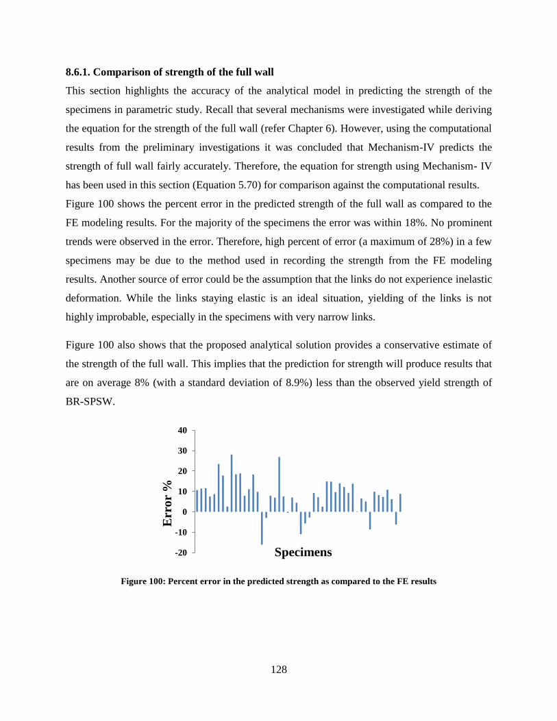
128

8.6.1. Comparison of strength of the full wall

This section highlights the accuracy of the analytical model in predicting the strength of the

specimens in parametric study. Recall that several mechanisms were investigated while deriving

the equation for the strength of the full wall (refer Chapter 6). However, using the computational

results from the preliminary investigations it was concluded that Mechanism-IV predicts the

strength of full wall fairly accurately. Therefore, the equation for strength using Mechanism- IV

has been used in this section (Equation 5.70) for comparison against the computational results.

Figure 100 shows the percent error in the predicted strength of the full wall as compared to the

FE modeling results. For the majority of the specimens the error was within 18%. No prominent

trends were observed in the error. Therefore, high percent of error (a maximum of 28%) in a few

specimens may be due to the method used in recording the strength from the FE modeling

results. Another source of error could be the assumption that the links do not experience inelastic

deformation. While the links staying elastic is an ideal situation, yielding of the links is not

highly improbable, especially in the specimens with very narrow links.

Figure 100 also shows that the proposed analytical solution provides a conservative estimate of

the strength of the full wall. This implies that the prediction for strength will produce results that

are on average 8% (with a standard deviation of 8.9%) less than the observed yield strength of

BR-SPSW.

Figure 100: Percent error in the predicted strength as compared to the FE results

-20

-10

0

10

20

30

40

Err

or

%

Specimens

129

8.6.2. Comparison of stiffness of the full wall

This section highlights the accuracy of the analytical model in predicting the stiffness of the

specimens in parametric study. The analytical model for the stiffness of the full wall was

developed on the basis of two ring-unit models: constrained and unconstrained ting models.

However, since the accuracy of the unconstrained ring model was restricted by fewer

assumptions, it was decided that the solution based on unconstrained ring-model will be used for

comparison to the computational results. The following paragraph discusses the accuracy of the

analytical solution and the cases in which it fails to predict the stiffness of the full wall within a

reasonable error limit.

Figure 101 shows that narrow links the predicted equation accurately predicts the stiffness of the

full wall (within 15% error). However, as the Ro/wl ratio decreases the percent error increases

significantly. This major deviation from the FE results is due to the fact that the analytical

solution ignores the width of the link and assumes the ring-link joint to be a point. Thus, wider

the link gets, the more deviation is seen from the actual solution. It was also found that the

proposed equation did not work well for very large radii plates (24 inches outer radius).

Irrespective of the Ro/wl ratio, all the specimens with 24 inches outer radius showed an error of

more than 30%.Other geometrical parameters did not play a major role in the accuracy of the

analytical model.

Additionally, it was also noted that the predicted stiffness was in most cases less than the actual

stiffness of the wall. This observation can be attributed to the fact that the derived equation for

stiffness does not include the stiffness of the links and the material at the boundary of the web

plate. It was found that the analytical solution predicted the results which were on an average

17% less that the observed stiffness of the full wall.

The final conclusion drawn from this comparison was that the proposed analytical model can be

used with good accuracy for Ro/wl ratios less than 2 and for plates with ring radius of 16 inches

or less.

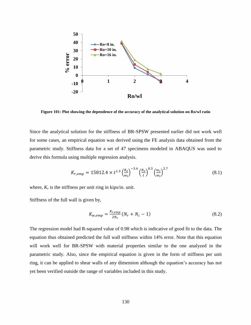
130

Figure 101: Plot showing the dependence of the accuracy of the analytical solution on Ro/wl ratio

Since the analytical solution for the stiffness of BR-SPSW presented earlier did not work well

for some cases, an empirical equation was derived using the FE analysis data obtained from the

parametric study. Stiffness data for a set of 47 specimens modeled in ABAQUS was used to

derive this formula using multiple regression analysis.

(

)

(

)

(

)

(8.1)

where, Kr is the stiffness per unit ring in kips/in. unit.

Stiffness of the full wall is given by,

(8.2)

The regression model had R-squared value of 0.98 which is indicative of good fit to the data. The

equation thus obtained predicted the full wall stiffness within 14% error. Note that this equation

will work well for BR-SPSW with material properties similar to the one analyzed in the

parametric study. Also, since the empirical equation is given in the form of stiffness per unit

ring, it can be applied to shear walls of any dimension although the equation’s accuracy has not

yet been verified outside the range of variables included in this study.

-20

-10

0

10

20

30

40

50

0 1 2 3 4

% e

rro

r

Ro/wl

Ro=8 in.

Ro=10 in.

Ro=16 in.

131

CHAPTER 9

FRACTURE PREDICTION AND FUTURE WORK

This section details the various approaches used to predict failure of the BR-SPSW. Predicting

fracture in the panel was challenging because of the complexity in the wall geometry and

limitations in currently available fracture prediction capability. Two models based on the void

growth mechanism which eventually leads to ductile fracture, have been discussed. Finally, a

finite element analysis based method has been used to model cracks. Shortcoming and challenges

of these approaches and recommendation for future work has been summarized.

9.1. SMCS MODEL

The initiation of ductile failure in steel is typically controlled by the growth and coalescence of

microvoids that nucleate around secondary particles, such as carbides or sulfides in the steel

matrix. Several models incorporate a combination of stress triaxiality and plastic strains to

predict fracture. One such model, first proposed by Hancock and Mackenzie 1977, and further

expanded by Panontin and Sheppard 1995, Rousselier 1987, Kanvinde and Deierlein 2006, and

Chi, Kanvinde et al. 2006 predicts fracture when equivalent plastic strain at any continuum point

exceeds a critical value. This failure criterion also referred stress modified critical strain (SMCS)

criterion is given by Equation 9.1.

(9.1)

In the above equation, T is the triaxiality ratio which is defined as the ratio of the equivalent or

Von Mises stress to the mean stress and is given by:

(9.2)

α is a material parameter that quantifies a material’s resistance to fracture. This parameter is

calibrated based on circumferential notched tension (CNT) bars.

Another crude, albeit effective way for comparing the potential for ductile fracture for two

configurations is to record their rupture index. The rupture index is defined as the ratio between

the plastic equivalent strain index and the ductile fracture strain multiplied by the material

constant α, such that,

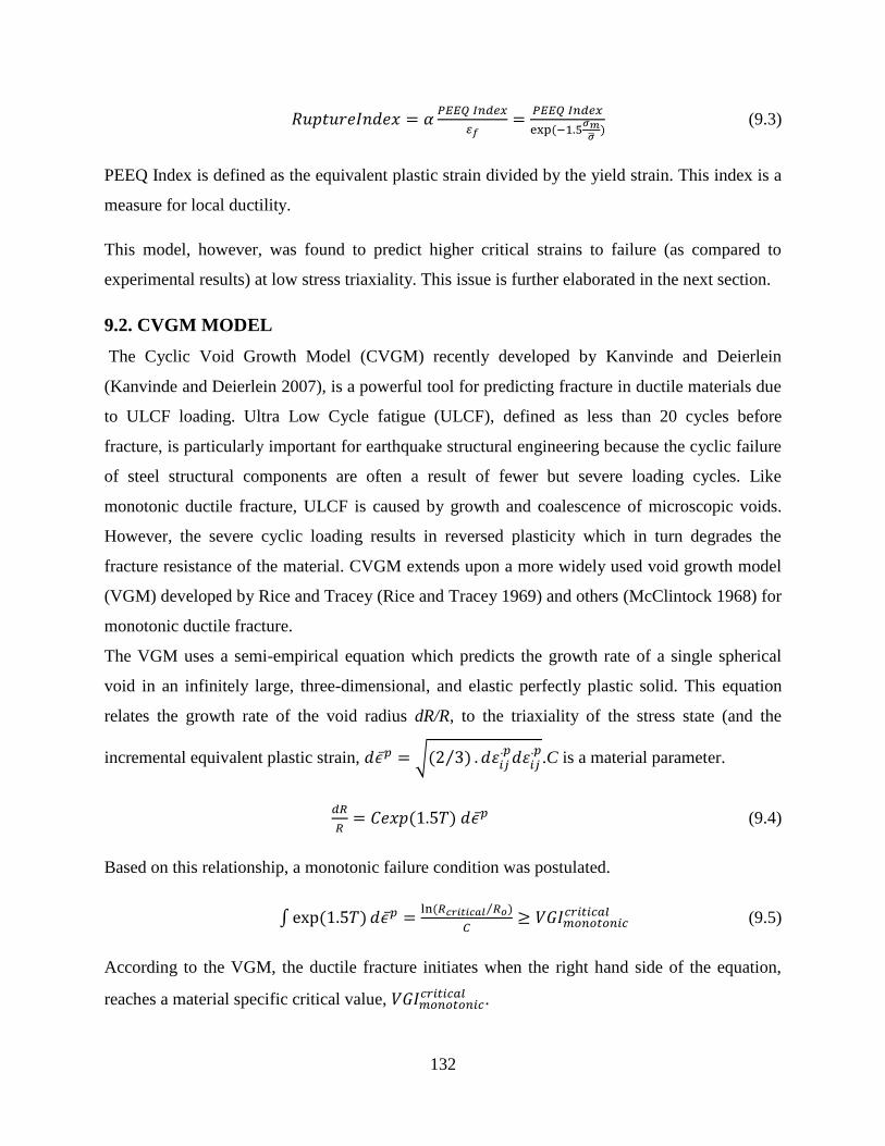
132

(9.3)

PEEQ Index is defined as the equivalent plastic strain divided by the yield strain. This index is a

measure for local ductility.

This model, however, was found to predict higher critical strains to failure (as compared to

experimental results) at low stress triaxiality. This issue is further elaborated in the next section.

9.2. CVGM MODEL

The Cyclic Void Growth Model (CVGM) recently developed by Kanvinde and Deierlein

(Kanvinde and Deierlein 2007), is a powerful tool for predicting fracture in ductile materials due

to ULCF loading. Ultra Low Cycle fatigue (ULCF), defined as less than 20 cycles before

fracture, is particularly important for earthquake structural engineering because the cyclic failure

of steel structural components are often a result of fewer but severe loading cycles. Like

monotonic ductile fracture, ULCF is caused by growth and coalescence of microscopic voids.

However, the severe cyclic loading results in reversed plasticity which in turn degrades the

fracture resistance of the material. CVGM extends upon a more widely used void growth model

(VGM) developed by Rice and Tracey (Rice and Tracey 1969) and others (McClintock 1968) for

monotonic ductile fracture.

The VGM uses a semi-empirical equation which predicts the growth rate of a single spherical

void in an infinitely large, three-dimensional, and elastic perfectly plastic solid. This equation

relates the growth rate of the void radius dR/R, to the triaxiality of the stress state (and the

incremental equivalent plastic strain, √ ⁄

.C is a material parameter.

(9.4)

Based on this relationship, a monotonic failure condition was postulated.

∫ ⁄

(9.5)

According to the VGM, the ductile fracture initiates when the right hand side of the equation,

reaches a material specific critical value, .

133

The CVGM extends the VGM so that the concepts used to develop it can be applied to ULCF

loading. The CVGM can be summed up by two equations. The first one presented in Equation

9.6, characterizes the fracture demand imposed on a material by ULCF loads. This equation

assumes that voids grow during tensile cycles and shrinks during compressive cycles. The nature

of a cycle (tensile or compressive) is defined by the sign (positive or negative) of the mean stress

at a material point.

∑ ∫ | |

∑ ∫ | |

(9.6)

In short, quantifies the effects of void growth and shrinkage due to ULCF loading.

The second equation (Equation 9.7) characterizes the fracture toughness of a material under

ULCF loads. It basically represents the capacity of material which decreases due to the strain

accumulation at the material point in question.

(

) (9.7)

Where λ is a material parameter that determines the rate at which ductile facture toughness

degrades and is the equivalent plastic strain that has accumulated up to the

beginning of each “tensile” excursion of loading.

The fracture is said to initiate when the fracture demand exceeds the fracture toughness or

capacity shown in Equation 9.8.

(9.8)

Once the failure mechanism was established, the CVGM was calibrated to the material test data.

This was done in two steps. First, was calibrated to monotonic noted bar tests

followed by the calibration of λ parameter to characterize degradation of the critical void ratio as

a function of accumulated strain. The calibration was done for seven different steel types. It was

noted that the notched cylindrical bars used for calibration provided high stress triaxiality values

(0.8-2.0).

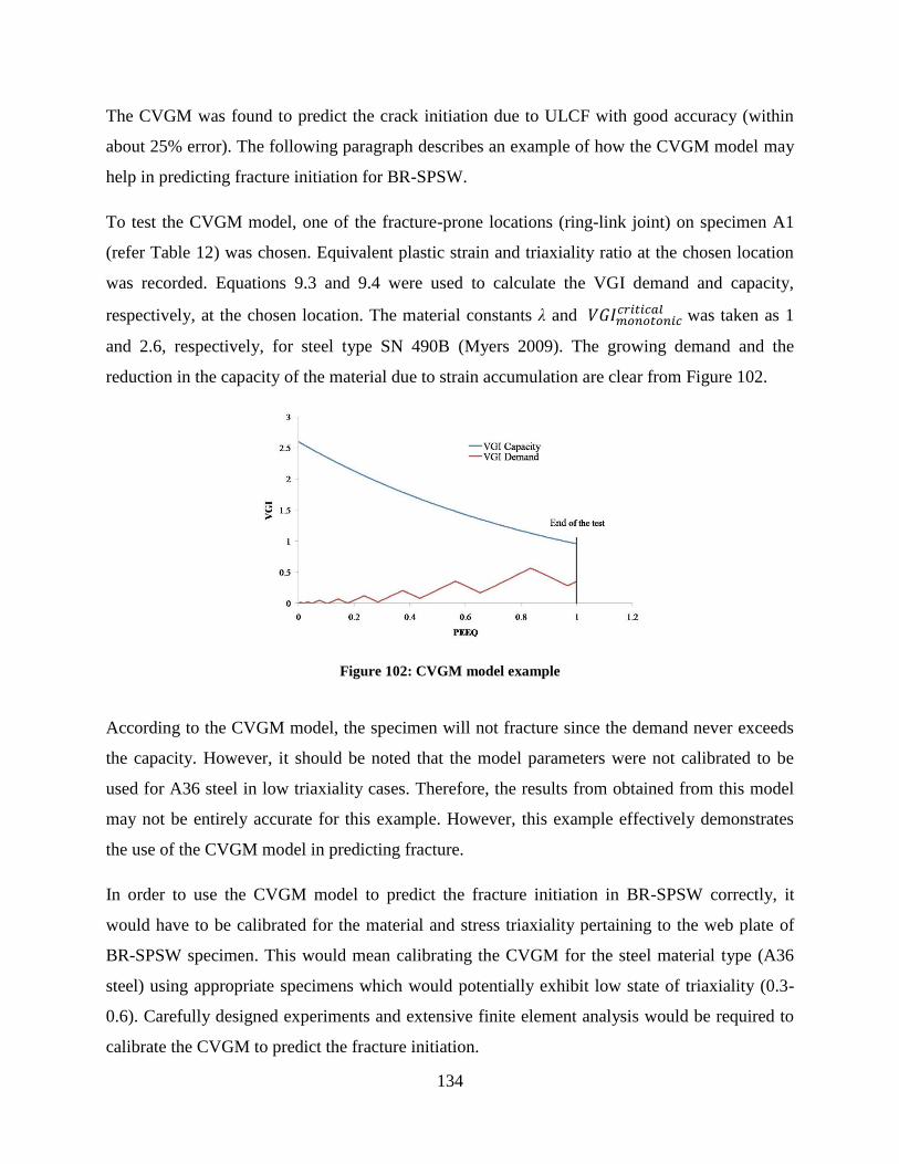
134

The CVGM was found to predict the crack initiation due to ULCF with good accuracy (within

about 25% error). The following paragraph describes an example of how the CVGM model may

help in predicting fracture initiation for BR-SPSW.

To test the CVGM model, one of the fracture-prone locations (ring-link joint) on specimen A1

(refer Table 12) was chosen. Equivalent plastic strain and triaxiality ratio at the chosen location

was recorded. Equations 9.3 and 9.4 were used to calculate the VGI demand and capacity,

respectively, at the chosen location. The material constants λ and was taken as 1

and 2.6, respectively, for steel type SN 490B (Myers 2009). The growing demand and the

reduction in the capacity of the material due to strain accumulation are clear from Figure 102.

Figure 102: CVGM model example

According to the CVGM model, the specimen will not fracture since the demand never exceeds

the capacity. However, it should be noted that the model parameters were not calibrated to be

used for A36 steel in low triaxiality cases. Therefore, the results from obtained from this model

may not be entirely accurate for this example. However, this example effectively demonstrates

the use of the CVGM model in predicting fracture.

In order to use the CVGM model to predict the fracture initiation in BR-SPSW correctly, it

would have to be calibrated for the material and stress triaxiality pertaining to the web plate of

BR-SPSW specimen. This would mean calibrating the CVGM for the steel material type (A36

steel) using appropriate specimens which would potentially exhibit low state of triaxiality (0.3-

0.6). Carefully designed experiments and extensive finite element analysis would be required to

calibrate the CVGM to predict the fracture initiation.

135

As discussed previously in the case of SMCS model, the major challenge while dealing with the

BR-SPSW would be the low triaxiality ratio it experiences. It has been identified (Fell 2008) that

at lower triaxiality states (0.33-0.75), the fracture may initiate on the surface and move inwards.

This is quite unlike the more constrained higher triaxiality cases where the fracture initiates

internally and then propagates outward. This shift in initiation location may impact the

mechanism of fracture. The research work by Bao and Wierzbicki (2004), lends an insight to the

dependence of fracture strain on triaxiality ratio for monotonic loading case. The authors

conducted a series of 11 tests on a particular aluminum alloy for which the triaxiality ratio

ranged from -0.3 to 0.95. A fracture locus was then developed which is shown in Figure 103. A

change in the fracture mechanism results in a slope discontinuity at triaxiality ratio of 0.4.

It is quite evident that there is a change in the fracture mechanism at lower state of triaxiality

(around 0.4). Extensive study in conjunction with suitably designed experiments would be

required to identify the different fracture mechanisms. This should eventually lead to the

development of a unified model that can predict fracture initiation for structures experiencing

any state of triaxiality.

Another challenge indirectly associated with these models is the high sensitivity of the

equivalent plastic strain to the mesh size. Thus, to ensure accurate values for equivalent plastic

strain, an appropriate mesh convergence analysis is highly recommended before settling on a

specific mesh size to obtain this particular data accurately.

Figure 103: Dependence of the equivalent strain to fracture on the stress triaxiality [from (Bao and

Wierzbicki 2004)]

136

9.3. EXTENDED FINITE ELEMENT MODELING (XFEM)

An extremely important aspect related to the fracture ductility of the BR-SPSW, which was

slightly touched upon during the course of this work was modeling cracks in the web plate.

Extended finite element method (XFEM) techniques were used to model cracks in single-ring

unit specimens subjected to monotonic loading. A brief discussion of the XFEM concept is

presented in the next paragraph followed by the results of crack modeling and how it can be

implemented in the full-scale BR-SPSW model.

Modeling discontinuities has always been a major challenge in the field of computational

mechanics. Cracks when modeled using standard finite element method (FEM) requires the FEM

mesh to conform to the crack geometry. In case of static or quasi-static evolving cracks or

dynamic crack propagation problems, a new mesh needs to be generated as the crack grows.

Additionally heavy mesh refinement is required at the discontinuity. This method therefore

proves to be computationally expensive. To ease difficulties in solving crack propagation

problems, XFEM was developed by Belytschko and Black (1999). This method requires the

application of an enrichment function in addition to the standard nodal DOF, to obtain

displacement interpolation locally in the domain of interest. These enrichment functions

represent the displacement jump across the crack face and the model singularity at the crack tip

and are known as the Heaviside function and Crack tip enrichment function respectively. The

XFEM displacement interpolation is represented by:

∑ [ ∑

] (9.9)

In the above equation, is the nodal DOF for conventional shape function . is the

enrichment function and is the nodal enriched DOF.

In terms of modeling in ABAQUS, the major advantage of this method is the ease of initial crack

definition. First, the mesh generation is independent of the crack. Also, there is no need of

partitioning the geometry as when a crack is represented explicitly. Secondly, XFEM allows

solution dependent crack initiation and propagation path so the crack path need not have to be

specified prior to the analysis. Moreover, the use of singular crack tip enrichment function results

in a much improved convergence rate as compared to standard FEM techniques. ABAQUS also

allows the damage modeling through predefined damage initiation and evolution criterion.

137

As mentioned in the beginning of the section, some basic ABAQUS analyses were done to

understand crack propagation in a single-ring unit subjected to monotonic loading. A 50%

maximum principal strain damage initiation criterion was used in the analyses. This was an

arbitrary criterion with the sole purpose of determining and controlling the location of the

fracture initiation. No pre-cracks were modeled. The initiation of the crack is shown in Figure

104. The crack initiates at joint of the link and the ring. This result was expected as the link-ring

joint is sharp and therefore prone to fracture.

A parametric study was done to investigate the effect of fillet radius (at the link-ring joint) on the

crack initiation and the behavior of the ring unit. The idea behind modeling crack in a single-ring

unit was to understand the post-fracture behavior of the unit. Most of the ABAQUS analysis

exhibited instability soon after the crack initiation. Several techniques were used to reduce this

instability but none of them worked well. The plots shown in Figure 105 terminate at

approximately the displacement at which the crack initiated.

A.

B. C.

Figure 104: Initiation of crack in a single-ring model

A few observations can be made from the parametric study. First, very evident from the plots is

the fact that with the increase in the fillet radius, the displacement at which cracks initiates

increases. There is also a slight increase in the capacity of the ring unit. The parametric study

138

also included the fillet radius of 3 inches. The behavior of the ring was however quite different

and hence the plot is separately shown in Figure 106. For this radius, the crack initiated at the

inner edge of the ring as shown in Figure 106 but did not fully develop and the analysis could

run without convergence issues. It was observed that once the crack started, the ring did not see

any deformation and it was the link that contributed to the capacity of the system. This prevented

the crack propagation. This kind of behavior is desirable for the ring-link system because the

system almost fully yielded before the crack propagated and degraded the system capacity.

However, it should be noted that this behavior is highly dependent on the damage

initiation/evolution criteria used for the analysis. It is therefore very important to use the most

suitable damage criteria. For this set of damage initiation/evolution criteria a fillet radius

between 25-36% (2-3 in. for this model) of the outer ring radius is desirable.

Figure 105: Plot showing the effect of fillet radius on crack initiation

0

20

40

60

80

100

120

140

0 1 2 3 4

Rea

ctio

n (

kip

s)

Horizontal Displacement (in.)

R=0

R=0.5

R=1

R=2

139

Figure 106: Force-displacement curve and crack initiation location for 3in. fillet model

The original intent was to use XFEM concepts on the full BR-SPSW wall to simulate the

initiation and propagation of cracks. Since the full wall model consists of many rings, it was

conjectured that this inherent redundancy would lead to good system behavior even if one ring

fractures. However, the implementation of this technique on the full wall still requires a

substantial amount of research work. First, the most appropriate damage initiation and evolution

criterion needs to be identified for BR-SPSW. It might be a maximum principle stress criteria,

principle strain criteria or a user-defined criteria formulated specifically for this geometry. This

might require some experimentation in conjunction with FE analysis. Secondly, there is also a

need for a more effective way of dealing with convergence problems.

0

50

100

150

200

0 1 2 3 4 5 6 7

Rea

ctio

n (

kip

s)

Horizontal Displacement (in.)

a: Plastic Hinge mechanism forms (link-ring joint)

b: Crack initiates

bc: Elastic deformation of the link

cd: Inelastic deformation of the link

a

b

c d

140

CHAPTER 10

EXPERIMENTATIONAL STUDY DESIGN

A parallel experimental program is being conducted at Virginia Tech to further validate the

concept behind BR-SPSW, investigate key parameters discussed in the previous section, and

provide data to compare with computational and analytical predictions. The tests will be

conducted on small-scale specimens and is expected to lend an insight to the ductility of the

system and potential for web plate fracture.

The test specimens will be modeled using similar methods as the computational study. A few

minor changes have been made in the geometry according to the test set-up. All sharp edges in

the plate geometry have been rounded off to (fillet radius equal to 20% of the outer ring radius)

reduce the potential of crack initiation. High quality water-jet cutting will be used to cut the

specific pattern for each specimen. A typical test specimen is shown in The schematic test-setup

for the experimental study is shown in Figure 108 .

Figure 107: A typical test specimen to be tested as a part of experimental study

For the experiment, a total of eight specimens were designed. One of these specimens was

chosen to be a solid plate with no perforations. This was done to compare the behavior of the

BR-SPSW with a typical solid shear wall. A detailed description of these specimens and

behavior related predictions associated with each of them is presented in Table 2027. Differences

between the predicted behavior and the experimental results will be investigated.

141

Table 20: Predicted behavior of the experiment Specimen 1 S

pec

imen

1

Plate thickness (t): 0.5 in.

Outer Ring Radius (Ro): 3.9 in.

Width of the link (wc): 1.52 in.

Predicted Strength:69.7 kips

Predicted Stiffness: 584 kips/in.

Table 21: Predicted behavior of the experiment Specimen 2

Sp

ecim

en 2






142


pec

imen

3







Sp

ecim

en 4



Width of the link (wc): 1.74 in

Predicted Strength:51 kips


143


pec

imen

5







Sp

ecim

en 6






144


pec

imen

7



Width of the link (wc): 1.52 in




Sp

ecim

en 8




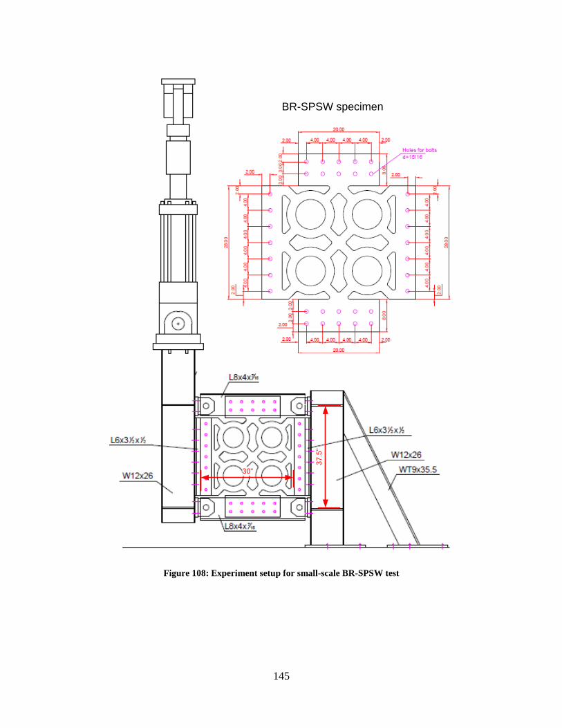
145

30"

37

.5"

BR-SPSW specimen

Figure 108: Experiment setup for small-scale BR-SPSW test

146

CHAPTER 11

SUMMARY AND CONCLUSIONS

This report includes the development of an efficient alternative to typical steel plate shear wall

followed by a detailed analysis of the proposed system. It highlights the major behavioral aspects

of the system and sensitivity of the system response to geometric features of the shear wall

system. The conclusions made in this report include the understanding of BR-SPSW system and

proposing analytical and computation models that can be used for the design of efficient and

high performance shear wall systems.

BR-SPSW concept has been devised which builds on the advantages of a typical steel plate shear

wall, but has improved seismic performance, reduced demands on the boundary elements and

allows simple shear beam-to-column connections. It employs a unique ring like cut-outs which

elongate into an ellipse when the shear plate is loaded laterally. This ring-effect reduces out-of-

plane buckling and lends tunability to BR-SPSW system. A brief summary of the work done in

developing this system and detailed conclusions drawn from this study of BR-SPSW is presented

below.

11.1. PRELIMINARY INVESTIGATIONS

A preliminary study of the BR-SPSW was undertaken to prove that the concept behind the ring-

like units in BR-SPSW would prevent excessive buckling of the web-plate and would resist

substantial fraction of lateral load without the use of moment connections. The study was done

by performing FE analysis on full wall and individual ring units using three dimensional finite

element models with shell elements.

From the analysis result of the full wall, it was observed that BR-SPSW exhibited relatively

fuller hysteresis as compared to the SPSW tested by Berman and Bruneau (2005). The pinching

was much less as compared to the aforementioned experimental result. It was further concluded

that BR-SPSW exhibits two modes of buckling. The specimens with larger rings exhibited a

combination of global tension field buckling and lateral torsional buckling of the rings, while the

specimens with smaller rings predominantly exhibit global tension field buckling.

147

Additionally, two single-ring models were devised in order to carefully capture the behavior of

the ring units in the full wall. These models namely, constrained and unconstrained ring models

were later used to understand the yielding mechanism of the rings in the full wall and for

developing analytical solutions for the strength and stiffness of the full wall. The force

deformation behavior of the unconstrained ring model also reinforced the fact that the when a

ring deforms into an ellipse the longitudinal and transverse deformations are nearly same. It was

found that up to an elongation of 20% of the ring diameter the effective Poisson’s ratio of the

ring is 1.0.

11.2. ANALYTICAL SOLUTION: STRENGTH OF THE FULL WALL

The analytical solution for the strength of the full wall was derived using the plastic mechanism

analysis. Deformation mechanics of individual ring units with different level of constraints was

studied. Four plastic mechanisms, some with and without plastic axial deformations, were

proposed to explain the inelastic behavior of the ring in the full wall. The analytical solution was

then compared to the preliminary finite element analysis results to establish the accuracy of the

solution.

Out of the various mechanisms put forth, Mechanism IV which was developed to explain the

mechanics of the constrained ring model agreed the best with the FE analysis results. This

mechanism assumed the formation of plastic hinges at the link-ring joint and ignored the

inelastic behavior of the links. It assumed that the top and bottom part of the rings act rigidly

(Refer Figure 33). The derived equation for strength was thus given by Equation 11.1.

√ (11.1)

On comparison with the FE analysis results from the parametric study, it was observed that the

proposed equation was conservative by an average of 8% with a standard deviation of 8.9%. As

mentioned above, the major source of the error is believed to be due to the assumption that the

links will remain fully elastic.

11.3. ANALYTICAL SOLUTION: STIFFNESS OF THE FULL WALL

The analytical solution for the stiffness of the full wall was developed along similar lines to the

strength of the wall. Both the constrained and unconstrained ring model was considered to study

148

the deformation mechanism. Castigliano’s Theorem was used for determining the displacements

for linear-elastic system based on partial derivatives of the strain energy with respect to the

generalized force in the direction of the displacement. The derived equation was then compared

to the initial stiffness (recorded in linear elastic region) of the specimens tested as the part of the

parametric study. While deriving the equation, the stiffness of the link was ignored to make the

solution simple.

Out of the two, the unconstrained ring model was restricted by fewer assumptions. It was

therefore used to predict the stiffness of BR-SPSW specimens. The stiffness of one ring unit

obtained from this model is given by,

(

{

})

(11.2)

Refer to Section 6.2 for the definition of the variables used in the equation.

The expression for the full wall is then given by,

(11.3)

On comparison to the FE analysis results, it was observed that the proposed equation works well

for models with narrow links and smaller radii. It was finally concluded that the proposed

analytical model can be used with good accuracy (within 15% error) for Ro/wlratio less than 2

with 16 inches outer radii or less. Overall, the predicted stiffness of the full wall was observed to

be on an average 17% less than the observed stiffness from the computational study.

Since the proposed analytical solution is complex and does not work for certain cases, an

empirical equation was derived using the FE analysis data obtained from the parametric study.

The empirical equation for the stiffness of a single ring unit is given by,

(

)

(

)

(

)

(11.4)

where, Kr is the stiffness per unit ring in kips/in. unit.

The stiffness of the ring unit can be translated to the stiffness of the full wall by using the

equation below.

149

(11.5)

11.4. EFFECT OF INITIAL IMPERFECTIONS

A small parametric study was conducted to investigate the effect of initial imperfections on the

performance of BR-SPSW when subjected to monotonic loading. In this study, specimens with

random imperfections and imperfections corresponding to the eigen buckling modes of the plate

were compared.

First, it was concluded that initial imperfections larger than L/100 result in significant reduction

in strength and stiffness and thus it is advisable to limit the imperfections to L/100. Secondly,

using random imperfections for modeling the plate was found to be acceptable. This was

concluded based on the observation that when compared to the models where the model was

built with an initial imperfection in the shape of the first eigen mode, the plates with random

imperfections exhibited very minor difference in the capacity and stiffness. On comparing the

effect of the shape of initial imperfections, it was found that the mode shape did not have a major

effect on the strength and stiffness of the plate.

A more palpable conclusion of the study was that as compared to the perfect geometry, the

specimens with any kind of initial imperfection exhibit reduced strength and stiffness. However,

this reduction is more severe in the plates with larger ring radius. Moreover, the system strength

and stiffness is not too sensitive to initial imperfections in the range of expected initial

imperfections (L/1000 to L/100). Typically, the expected initial imperfections might be L/500

based on typical tolerances for out-of-straightness for a new construction. This lack of sensitivity

is beneficial because the wall behavior won’t change significantly if one of the web plates has

more imperfections than another.

11.5. PARAMETRIC STUDY

The parametric study was done to build on the results of the preliminary study. It aimed at

characterizing the influence of geometric features of the wall on the overall behavior of the

system. A set of input and output parameters was defined for the parametric study. A set of

behavioral trend plots were generated as an aid for the design process. Major conclusions drawn

from these plots are summarized below.

150

Thickness of the web plate plays an important role in all the behavioral aspects of BR-

SPSW. A thicker plate exhibits a relatively fuller hysteretic behavior and does not

experience substantial strength and stiffness reduction. This results in relatively much

larger energy dissipation. A thinner plate experiences buckling at earlier stage and

therefore exhibits a much smaller energy dissipation ratio. Moreover, thinner plates more

often exhibit lateral torsional buckling of the rings in conjunction to the global tension

field buckling which was shown to cause pinching in the hysteretic behavior of the shear

wall. Needless to say, thicker web plates also result in higher strength and stiffness of the

full wall. Additionally, it was observed that increase in thickness increases the drift at

which the shear wall system yields globally.

As expected, the behavior of BR-SPSW is highly sensitive to the size of the ring units.

This is because the ring size is a major factor in determining the type of buckling the

web-plate will experience. It was concluded that smaller radii rings resulted in global

tension field buckling of the plate. On the contrary, BR-SPSW with larger radii

experienced local torsional buckling of the rings in conjunction to the global tension field

buckling. This difference in the buckling behavior of the wall influences the total energy

dissipation and the energy dissipation ratio alike. It is hypothesized that lateral torsional

buckling of the rings results in pinching of the hysteresis curve and thus reduces the

energy dissipation capacity of the wall. This hypothesis was based on the idea that the

distortion in the ring units caused by the local torsional buckling prevents the natural

elongation of the rings into an ellipse, which was the basic idea behind BR-SPSW. This

degrades the behavior of individual ring units and in turn the full wall.

The parametric results also showed that although the strength per ring increases with

increase in radius, the strength of the full wall with given dimensions may not necessarily

be larger for larger radii ring models. The only major advantage of using a larger radius

ring is the reduced cutting cost. It was observed that decreasing the ring radii

exponentially increases the cutting cost of BR-SPSW. However, in all other aspects web-

plates with smaller radii exhibit much better behavior.

Another input parameter that had a major influence on the hysteretic behavior of the full

wall was Ro/wc ratio. Based on the FE analysis, it was observed that keeping Ro/wc ratio

in the range of 2.5-3.33, results in fuller hysteretic behavior and higher energy dissipation

151

ratio. An increase in the Ro/wc ratio results in a tremendous increase in the buckling ratio,

indicating that specimens with wider rings suffer from lateral torsional buckling of the

rings which has been proved to be undesirable. An increase in the Ro/wc ratio, however,

also results in an exponential decrease in the strength and stiffness/ring. Additionally, the

cost of cutting also increases slightly with the increase in this ratio. It can be concluded

that keeping the ratio around 2.5-3.33 would result in an optimum design.

Ro/wl ratio has a similar influence on the strength and stiffness per ring as the Ro/wc ratio.

However, Ro/wl ratio has a much less significant effect on the system behavior as

compared to the Ro/wc ratio. Increasing the Ro/wl ratio slightly reduces the energy

dissipation capacity of the full wall but has not major influence on the energy dissipation

ratio. The cutting cost of the plate also slightly increases with an increase in the Ro/wl

ratio. Using a Ro/wl ratio less than 3 is recommended since a very narrow link is prone to

inelastic deformation which is undesirable.

The ring slenderness ratio (Ro/t and wc/t) has a major influence on the buckling behavior

of the plate. It was observed that an increase in slenderness ratio results in a substantial

decrease in the total dissipated energy and the buckling ratio. The slenderness ratio of the

rings must be controlled for the design of more efficient BR-SPSW.

11.6. GENERAL OBESERVATIONS AND CONCLUSIONS

Some general conclusions drawn from the study are presented below.

The concept of BR-SPSW was largely validated. The buckling of the web-plate was

considerably reduced with substantial resistance during load reversals. A majority of the

specimens tested in the parametric study exhibited relatively full hysteretic behavior.

Energy dissipation ratio as high as 0.78 was observed, which indicates little pinching and

high energy dissipation. The hypothesis regarding the ring deforming into an ellipse to

reduce buckling works to a large extent. However, since this “ring effect” is an idealized

concept, it was found to not to fully prevent buckling. The following paragraphs highlight

the reasons for this deviation in the behavior of BR-SPSW.

The major reason why BR-SPSW does not fully prevent buckling is due to the inelastic

deformation of the links joining the rings. This results in non-uniform distribution of

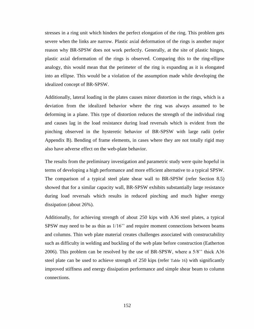
152

stresses in a ring unit which hinders the perfect elongation of the ring. This problem gets

severe when the links are narrow. Plastic axial deformation of the rings is another major

reason why BR-SPSW does not work perfectly. Generally, at the site of plastic hinges,

plastic axial deformation of the rings is observed. Comparing this to the ring-ellipse

analogy, this would mean that the perimeter of the ring is expanding as it is elongated

into an ellipse. This would be a violation of the assumption made while developing the

idealized concept of BR-SPSW.

Additionally, lateral loading in the plates causes minor distortion in the rings, which is a

deviation from the idealized behavior where the ring was always assumed to be

deforming in a plane. This type of distortion reduces the strength of the individual ring

and causes lag in the load resistance during load reversals which is evident from the

pinching observed in the hysteretic behavior of BR-SPSW with large radii (refer

Appendix B). Bending of frame elements, in cases where they are not totally rigid may

also have adverse effect on the web-plate behavior.

The results from the preliminary investigation and parametric study were quite hopeful in

terms of developing a high performance and more efficient alternative to a typical SPSW.

The comparison of a typical steel plate shear wall to BR-SPSW (refer Section 8.5)

showed that for a similar capacity wall, BR-SPSW exhibits substantially large resistance

during load reversals which results in reduced pinching and much higher energy

dissipation (about 26%).

Additionally, for achieving strength of about 250 kips with A36 steel plates, a typical

SPSW may need to be as thin as 1/16’’ and require moment connections between beams

and columns. Thin web plate material creates challenges associated with constructability

such as difficulty in welding and buckling of the web plate before construction (Eatherton

2006). This problem can be resolved by the use of BR-SPSW, where a 5/8’’ thick A36

steel plate can be used to achieve strength of 250 kips (refer Table 16) with significantly

improved stiffness and energy dissipation performance and simple shear beam to column

connections.

153

Although not yet experimentally proven, another major advantage of BR-SPSW is

expected to be the redundancy provided by the arrays of rings. This implies that if a one

ring fracture during loading, the web plate is not expected to see major deterioration in its

capacity. In a typical SPSW, fracture initiation generally leads to substantial decrease in

the system capacity and in turn leads to the failure of the specimen (Berman and Bruneau,

2005).

Analytical and empirical solutions for the strength and stiffness of BR-SPSW were

derived. These solutions in conjunction with the trend plots presented in Section 8.4

provide a powerful tool that can be used for designing BR-SPSW.

The study presented in this report is purely based on computational observations.

Experiments are required and will be conducted in the near future to further validate the

concept and the computational modeling. Good behavior is expected for the selected

specimens as predicted by finite element models (Refer Table 20).

154

REFERENCES

ABAQUS Version 6.10 documentation, Dassault Systems, 10, Rue Marcel Dassault, 78140

Velizy-Villacoublay, France, 6th Edition.

Ahmed, A., Extended Finite Element Method(XFEM)- modeling arbitrary discontinuities and

failure analysis, Master’s thesis, The Institute for Advanced Study of Pavia, Pavia, Italy (April

2009).

American Institute of Steel Construction (AISC), Seismic Provisions for Structural Steel

Buildings AISC 341-10, (2005).

Astaneh, A., Seismic behavior and design of steel shear walls, In proceedings of SEOANC

Seminar, Structural Engineers Assoc. of Northern California, San Francisco, California, 2001.

Baldelli, J.A., Steel shear walls for existing buildings, Engineering Journal of the American

Institute of Steel Construction 20 (1983) 70-77.

Bao, Y., Wierzbicki, T., On fracture locus in the equivalent strain and stress triaxiality space,

International Journal of Mechanical Sciences 46 (1) (2004) 81-98.

Berman, J.W., Bruneau, M., Experimental investigation of light-gauge steel plate shear walls for

the seismic retrofit of buildings, Technical Report MCEER-03-0001, Multidisciplinary Center

for Earthquake Engineering Research, Buffalo, NY (May 2003).

Berman, J.W., Bruneau, M., Steel Plate Shear Walls are not plate girders, Engineering Journal of

the American Institute of Steel Construction, Third Quarter, (2004) 95-106.

Berman, J.W., Celik, O.C., Bruneau, M., Comparing hysteretic behavior of light-gauge steel

plate shear walls and braced frames, Engineering Structures 27 (3) (2005) 475-485.

Bruneau, M., Berman, J., Lopez-Garcia, D., Vian, D., A Review of Steel Plate Shear Wall

Design Requirements and Research, Engineering Journal of the American Institute of Steel

Construction, 44(1) 2007 27-34.

Berman, J.W., Seismic behavior of code designed steel plate shear walls, Journal of Engineering

Structures 33 (2011) 230-244.

Caccese, V., Elgaaly, M., Du, C., Experimental study of thin steel plate shear walls under cyclic

load, Journal of Structural Engineering (ASCE) 119 (2) (1983) 573-587.

155

Caccese, V., Elgaaly, M., Du, C., Postbuckling behavior of steel-plate shear walls under cyclic

loads, Journal of Structural Engineering (ASCE) 119 (2) (1993) 588-605.

Chen, J.S., Jhang, C., Experimental study of low-yield-point steel plate shear wall under in-plane

load, Journal of Constructional Steel Research 67 (2011) 977-985.

Chen, W.F., Han, D.J., Plasticity for Structural Engineers, J. Ross Publishing, 2007.

Chi, W. M., Kanvinde, A. M., Deierlein, G. G., Prediction of ductile fracture in steel connections

using SMCS criterion, Journal of Structural Engineering 132 (2) (2006) 171-181.

Ciampi, V., Samuelli-Ferretti, A., Energy dissipation in buildings using special bracing systems,

In proceedings of the 9th European Conference on Earthquake Engineering, Vol. 3 of 9-18,

Moscow, Russia, 1990.

Ciampi, V., Arcangeli, M., Perno, S., Characterization of the low-cycle fatigue life of a class of

energy dissipating devices, In proceedings of the 2nd

European Conference on Structural

Dynamics (EURODYN '93), Vol. 1 of 337-X, Trondheim, Norway, 1993, pp. 137-144.

Cortes, G., Liu, J., Steel slit panel configurations, In proceeding of the 14th World Conference

on Earthquake Engineering, Beijing, China, 2008.

Driver, R.G., Kulak, G.L., Kennedy, D.J.L., Elwi, A.E., Seismic behavior of steel plate shear

walls, Structural Engineering Report 215, Department of Civil and Environmental Engineering,

University of Alberta, Edmonton, Alberta, Canada (February 1997).

Eatherton, M.R., Design and construction of steel plate shear walls, In proceedings of the 8th

U.S. National Conference on Earthquake Engineering, San Francisco, California, 2006.

Elgaaly, M., Thin steel plate shear walls behavior and analysis, Thin Walled Structure 32 (1998)

151-180.

Fell, B. V., Large-scale testing and simulation of earthquake-induced ultra low cycle fatigue in

bracing members subjected to cyclic inelastic buckling, Phd dissertation, University of

California, Davis, CA (2008).

Hancock, J. W., Mackenzie, A. C., On the mechanics of ductile fracture in high strength steels

subjected to multiaxial states of stress, Journal of mechanics and physics of solids 14 (1977) 147-

169.

156

Hitaka, T. and Matsui, C., Experimental study on steel shear wall with slits, Journal of Structural

Engineering (ASCE) 129 (5) (2003) 586-595.

Hitaka, T., Matsui, C., Tsuda, K., Sadakane, Y., Elastic-plastic behavior of buildings of steel

frame with steel bearing wall with slits, In proceeding of the 12th World Conference on

Earthquake Engineering, no. 0833, Auckland, New Zealand, 2000.

Hitaka, T., Matsui, S., Seismic performance of steel shear wall with slits integrated with multi-

story composite moment frame, In proceedings of the 5th International Conference on Behaviour

of Steel Structures in Seismic Areas, Yokohama, Japan, 2006.

Kanvinde, A. M., Deierlein, G. G., Cyclic void growth model to assess ductile fracture initiation

in structural steels due to ultra low cycle fatigue, Journal of Engineering Mechanics 133(6)

(2007) 701-712.

Lubell, A., Prion, H., Ventura, C., Rezai, M., Unstiffened steel plate shear wall performance

under cyclic loading, Journal of Structural Engineering (ASCE) 126 (4) (2000) 453-460.

Ma, X., Borchers, E., Peña, A., Krawinkler, H., Deierlein, G., Design and behavior of steel shear

plates with openings as energy-dissipating fuses, Internal report, Blume Earthquake Engineering

Center, Stanford University, Stanford, California (2010).

Martinez-Rueda, J.E., On the evolution of energy dissipation devices for seismic design,

Earthquake Spectra 18 (2) (2002) 309-346.

McCloskey, D.M., Steel slit panels for lateral resistance of steel frame buildings, MS thesis,

Department of Civil Engineering, Purdue University, West Lafayette, Indiana. (2006).

Moes, N., DolBow, J., Belytschko, T. A finite element method for crack growth without

remeshing, International Journal for Numerical Methods in Engineering, 46 (1999) 131-150.

Moghini, H., Driver, R.G., Effect of regular perforation patterns on steel plate shear wall column

demands, In proceedings of Structures Congress (ASCE), Las Vegas, Nevada, United States,

2011, pp. 2917-2928.

Myers, A., Testing and probabilistic simulation of ductile fracture initiation in structural steel

components and weldments, Phd dissertation, Stanford University, Stanford, CA (2009).

157

Panontin, T. L., Sheppard, S. D., An experimentally verified finite element study of the stress-

strain response of crack geometries experiencing large-scale yielding, In proceedings of the 27th

International Symposium on Fatigue and Fracture Mechanics, Vol. 27, ASTM Committee,

Williamsburg, Virginia, 1995, pp. 216-242.

Rice, J. R., Tracey, D. M., On the ductile enlargement of voids in triaxial stress fields, Journal of

Mechanics Physics Solids 17 (3) (1969) 201-217.

Roberts, T., Sabouri-Ghomi, S., Hysteretic characteristics of unstiffened perforated steel plate

shear panels, Thin-Walled Structures 14 (2) (1992) 139-151.

Rogers, C., and Morrison, T., Ductile brace fuses for cost effective design of brace steel frames,

In proceedings of North American Steel Construction Conference, Pittsburgh, Pennsylvania,

2011.

Rousselier, G., Ductile fracture models and their potential in local approach of fracture, Nuclear

Engineering and Design 105 (1) (1987) 97-111.

Sabelli, R., Bruneau, M., Design Guide 20: Steel Plate Shear walls, American Institute of Steel

Construction (2006).

Schumacher, A., Grondin, G.Y., Kulak, G.L., Connection of infill panels in steel plate shear

Walls, Canadian Journal of Civil Engineering 26 (1992) 549-563.

Tanamal, A., Eatherton, M., Hajjar, J. F., Controlled rocking of steel-framed buildings with

replaceable energy dissipating fuses fuse material coupons – tension tests, Tech. Rep. 61801,

University of Illinois at Urbana-Champaign, Urbana, Illinois (March 2009).

Thorburn, L.J., Kulak, G.L., Montgomery, C.J., Analysis of steel plate shear walls., Structural

Engineering Report 107, Department of Civil Engineering, University of Alberta, Edmonton,

Alberta, Canada (May 1983).

Timler, P.A., Kulak, G.L., Experimental study of steel plate shear walls, Structural engineering

report 114, Department of Civil Engineering, University of Alberta, Edmonton, Alberta, Canada

(1983).

Timler, P.A., Design procedures development, analytical verification, and cost evaluation of

steel plate shear wall structures, Technical report 98-01, Earthquake Engineering Research

Facility, University of British Columbia, Vancouver, British Columbia, Canada (1998).

158

Tipping, S., B. Stojadinovic, S., Innovative corrugated steel shear walls for multi-story

residential buildings, in: In proceedings of the 14th World Conference on Earthquake

Engineering, 2008.

Tromposch, E.W., Kulak, G.L., Cyclic and static behavior of thin panel steel plate shear walls,

Structural Engineer Report 145, Department of Civil Engineering, University of Alberta,

Edmonton, Alberta, Canada (April 1987).

Tyler, R. G.,, Further notes on a steel energy-absorbing element for braced frameworks, Bulletin

of the New Zealand National Society for Earthquake Engineering 18 (3) (1985) 270-279.

Vian, D., Bruneau, M., Steel plate shear wall for seismic design and retrofit of building

structures, MCEER Technical Report 05-0010, Multidisciplinary Center for Earthquake

Engineering Research, University at Buffalo (2005).

Vian, D., Bruneau, M.,, Testing of special LYS steel plate shear walls, In proceedings of the 13th

World Conference on Earthquake Engineering, no. 978, Vancouver, B.C., Canada, 2004.

Wagner, H., Flat sheet metal girder with very thin metal web, Technical Memo 604-606,

National Advisory Committee for Aeronautics (NACA), Washington, D.C. (1931).

Xue, M., Lu, L., Interaction of Infilled Steel Shear Wall Panels with Surrounding Frame

Members. 1994 Annual Task Group Technical Session, Structural Stability Research Council

report on current research activities, Lehigh University, Bethlehem, PA, June 1994.

Zeinoddini-Meimand, V., Geometric imperfections in cold-formed steel members, PhD

dissertation, Johns Hopkins University (2011).

159

APPENDIX A: TREND PLOTS

This appendix compiles the trend plots generated for the output variables of the system with

respect the geometrical features of the BR-SPSW system. These trend plots can be used for the

design of BR-SPSW.

APPENDIX A1

BEHAVIOR TRENDS FOR FULL-WALL STRENGTH

(a)

(b)

(c)

(d)

Ro/wc=3.33 Ro/wl=2 Ro/wc=3.33 Ro/wl=2

Ro/wc=3.33 Ro/wl=2

Ro/wc=3.33 Ro/wl=2

160

(e)

(f)

Figure A.109: Trend plots for strength per ring

APPENDIX A2

BEHAVIOR TRENDS FOR FULL-WALL STIFFNESS

(a)

(b)


Ro=10 in. Ro/wl=2 Ro=10 in. Ro/wc=3.33

161

(c)

(d)

(e)

(f)

Figure A.110: Trend plots for stiffness per ring


Ro=10 in. Ro/wl=2 Ro=10 in. Ro/wc=3.33

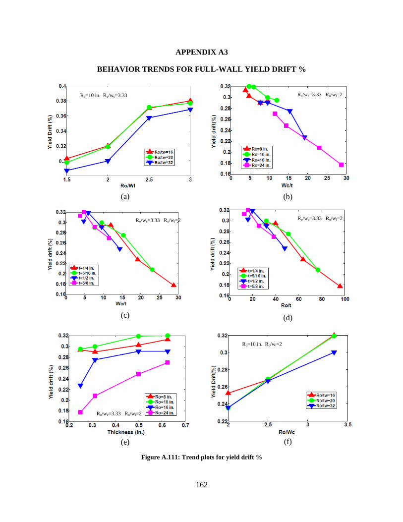
162

APPENDIX A3

BEHAVIOR TRENDS FOR FULL-WALL YIELD DRIFT %

(a)

(b)

(c)

(d)

(e)

(f)

Figure A.111: Trend plots for yield drift %

Ro/wc=3.33 Ro/wl=2

Ro/wc=3.33 Ro/wl=2

Ro/wc=3.33 Ro/wl=2

Ro/wc=3.33 Ro/wl=2

Ro=10 in. Ro/wl=2


163

APPENDIX A4

BEHAVIOR TRENDS FOR TOTAL DISSIPATED ENERGY

(a)

(b)

(c)

(d)

(e)

(f)

Figure A.112: Trend plots for total dissipated energy

Ro/wc=3.33 Ro/wl=2

Ro/wc=3.33 Ro/wl=2

Ro/wc=3.33 Ro/wl=2

Ro=10 in. Ro/wl=2


Ro/wc=3.33 Ro/wl=2


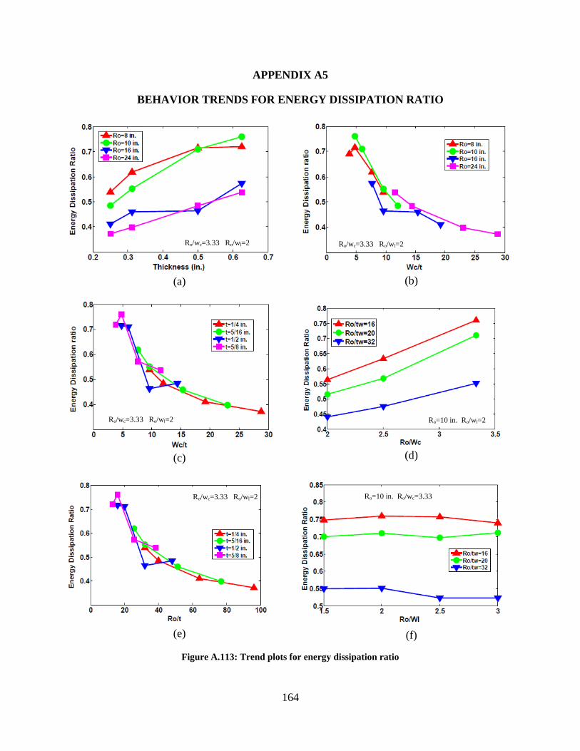
164

APPENDIX A5

BEHAVIOR TRENDS FOR ENERGY DISSIPATION RATIO

(a)

(b)

(c)

(d)

(e)

(f)

Figure A.113: Trend plots for energy dissipation ratio


Ro/wc=3.33 Ro/wl=2

Ro/wc=3.33 Ro/wl=2

Ro=10 in. Ro/wl=2


165

APPENDIX A6

BEHAVIOR TRENDS FOR BUCKLING RATIO

(a)

(b)

(c)

(d)

(e)

Figure A.114: Trend plots for buckling ratio

Ro/wc=3.33 Ro/wl=2

Ro/wc=3.33 Ro/wl=2


Ro=10 in. Ro/wl=2

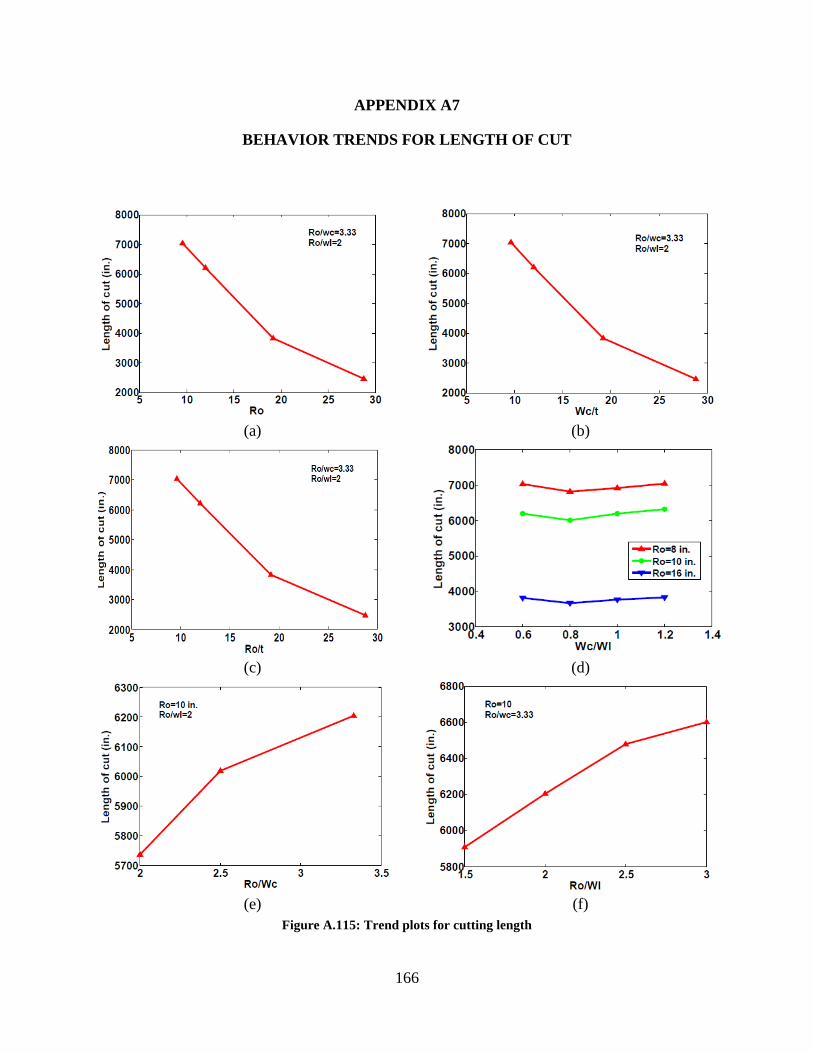
166

APPENDIX A7

BEHAVIOR TRENDS FOR LENGTH OF CUT

(a)

(b)

(c)

(d)

(e)

(f)

Figure A.115: Trend plots for cutting length

167

APPENDIX B: HYSTERETIC PLOTS

This appendix tabulates the hysteresis plots generated for each test specimen which was the part

of the parametric study.

(a)

(b)

(c)

(d)

168

(e)

(f)

(g)

(h)

(i)

(j)

169

(k)

(l)

(m)

(n)

(o)

(p)

170

(q)

(r)

(s)

(t)

(u)

(v)

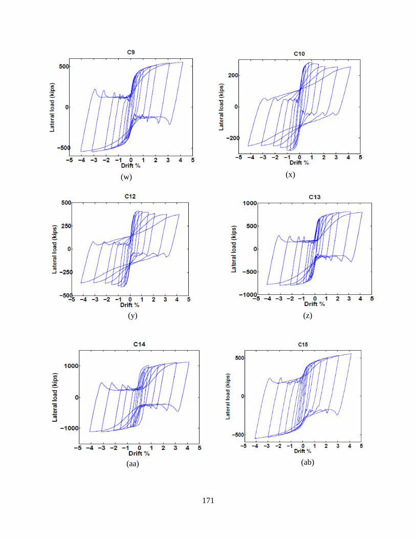
171

(w)

(x)

(y)

(z)

(aa)

(ab)

172

(ac)

(ad)

(ae)

(af)

(ag)

(ah)

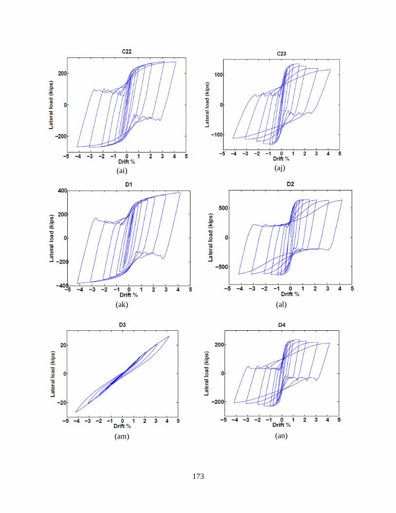
173

(ai)

(aj)

(ak)

(al)

(am)

(an)

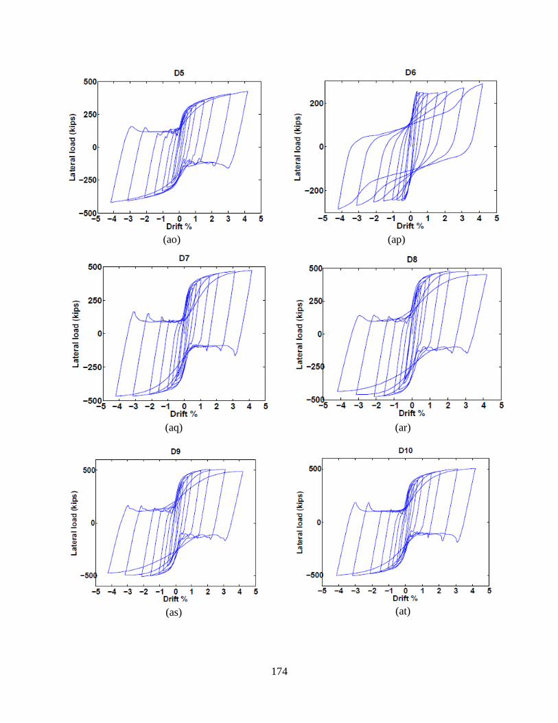
174

(ao)

(ap)

(aq)

(ar)

(as)

(at)

175

(au)

(av)

Figure A.116: Hysteresis plots for specimens

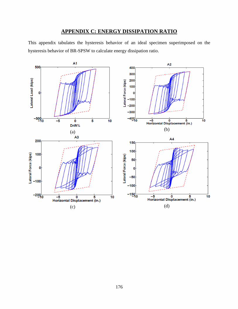
176

APPENDIX C: ENERGY DISSIPATION RATIO

This appendix tabulates the hysteresis behavior of an ideal specimen superimposed on the

hysteresis behavior of BR-SPSW to calculate energy dissipation ratio.

(a)

(b)

(c)

(d)

177

(e)

(f)

(g)

(h)

(i)

(j)

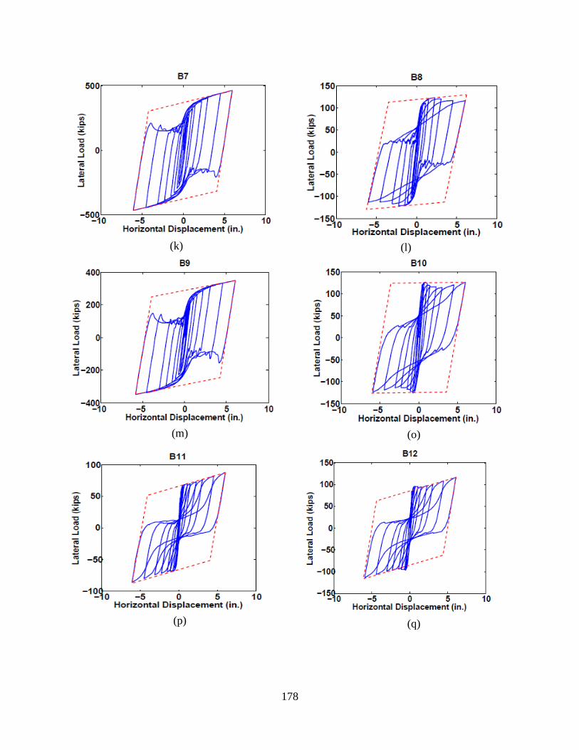
178

(k)

(l)

(m)

(o)

(p)

(q)

179

(r)

(s)

(t)

(u)

(v)

(w)

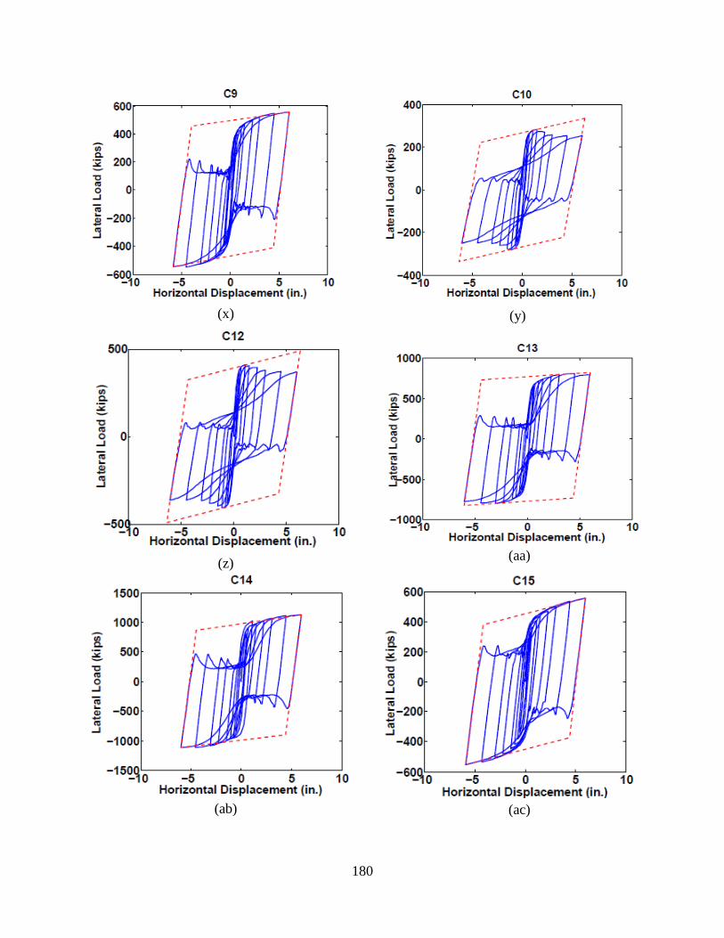
180

(x)

(y)

(z)

(aa)

(ab)

(ac)

181

(ad)

(ae)

(af)

(ag)

(ah)

(ai)

182

(aj) (ak)

(al)

(am)

(an)

(ao)

183

(ap)

(aq)

(ar)

(as)

(at)

(au)

184

(av)

Figure A.117: Plots for the calculation of energy dissipation ratio

185

APPENDIX D: STRENGTH CALCULATION

This appendix tabulates the force-displacement plot for all the specimens generated for the

purpose of strength calculation of the full wall.

(a)

(b)

(c)

(d)

(e)

(f)

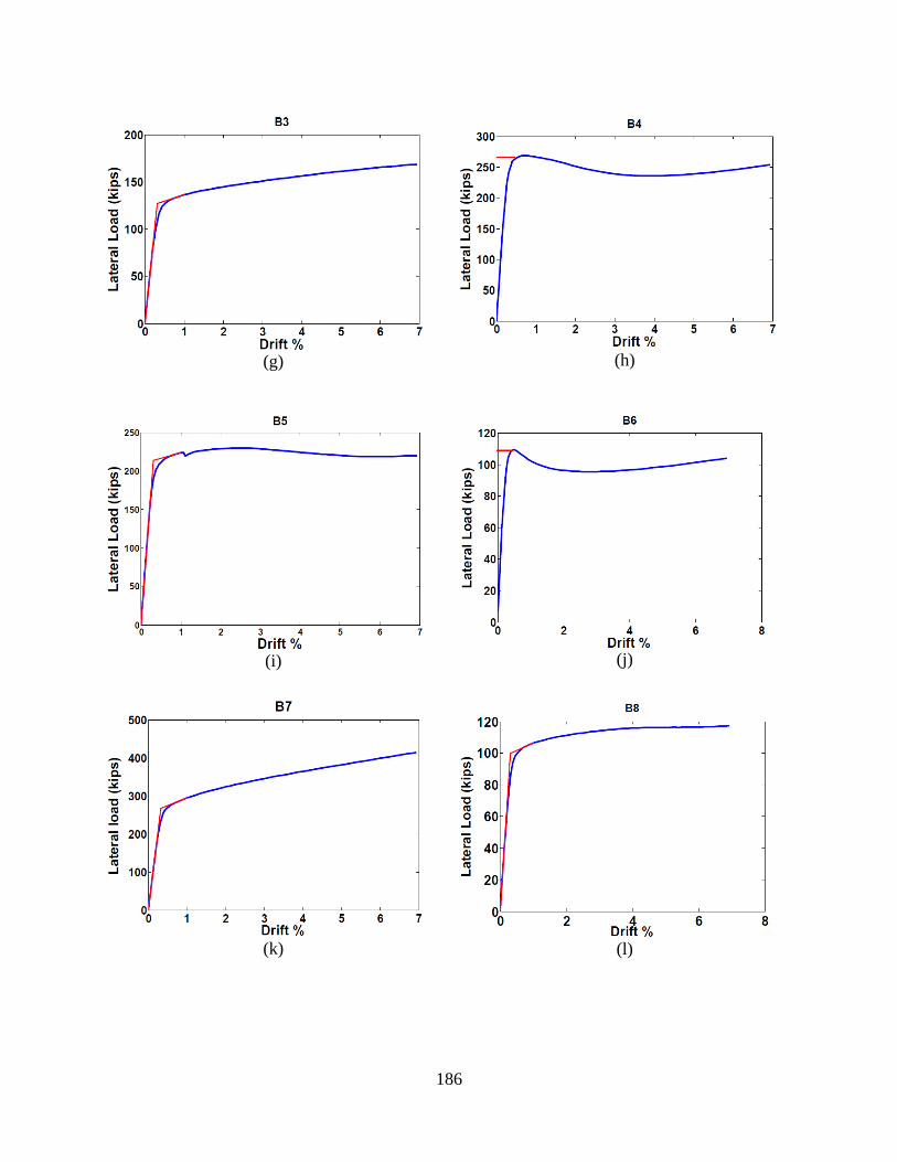
186

(g)

(h)

(i)

(j)

(k)

(l)

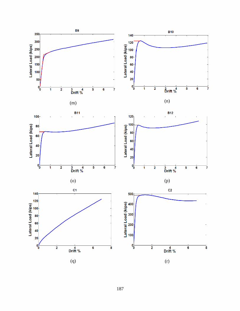
187

(m)

(n)

(o)

(p)

(q)

(r)

188

(s)

(t)

(u)

(v)

(w)

(x)

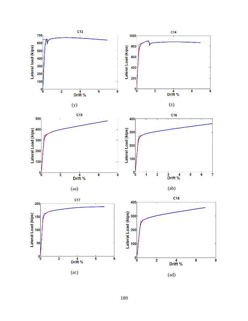
189

(y)

(z)

(aa)

(ab)

(ac)

(ad)

190

(ae)

(af)

(ag)

(ah)

(ai)

(aj)

191

(ak)

(al)

(am)

(an)

(ao)

(ap)

192

(aq)

(ar)

(as)

(at)

(au)

Figure A.118: Plots showing the method for calculation of full wall strength

193

APPENDIX E: COPYRIGHTED FIGURES

This appendix lists citations for copyrighted works (figures). Fair use determination for each

figure is attached separately.

Figure 1: A four-story SPSW system [from (Berman and Bruneau 2004)]

Figure 2: Force-displacement plot for a typical steel plate shear wall system [from (Berman,

Celik and Bruneau 2005)]

Figure 3: Force-displacement plot for a shear wall web plate [from (Berman, Celik and Bruneau

2005)]

Figure 5: Diagrammatic representation of Strip Model [from (Lubell et al. 2000)]

Figure 6: Diagrammatic representation of multi-angle strip model [from (Lubell et al. 2000)]

Figure 7: Infill panel connection details tested [from (Schumacher, Grondin and Kulak 1999)]

Figure 9: Perforated steel plate shear walls [from (Roberts et al. 1992 and Vian et al. 2005)]

Figure 10: Steel plate walls with rectangular slits [from (Hitaka et al. 2006)]

Figure 11: Panel with butterfly fuse [from (Borchers, Peña, Krawinkler, and Deierlein 2010)]

Figure 12: Yielding frame with constant cross-section [from (Tyler 1985)]

Figure 13: Yielding frame with varying width [from (Ciampi and Samuelli-Ferretti 1990)]

Figure 14: Yielding frame with varying depth [from (Ciampi and Samuelli-Ferretti 1990)]

Figure 15: Yielding frame with complementary plates [from (Ciampi and Samuelli-Ferretti

1990)]

Figure 16: Ring fuse [from (Rogers and Morrison 2011)]

Figure 42: axial-bending interaction curve for rectangular cross-section [from (Chen and Han

2007)]

Figure 103: Dependence of the equivalent strain to fracture on the stress triaxiality [from (Bao

and Wierzbicki 2004)]

computational simulation and analytical … · buckling resistant steel plate shear wall (br-spsw)...

Documents