Computational ScienceLaboratory Technical Report

CSL-TR-3-2013October 18, 2018

Alexandru Cioaca,Adrian Sandu, and Eric de Sturler

Efficient methods for computingobservation impact

in 4D-Var data assimilation

Computational Science LaboratoryComputer Science Department

Virginia Polytechnic Institute and State UniversityBlacksburg, VA 24060Phone: (540)-231-2193Fax: (540)-231-6075

Email: sandu@cs.vt.eduWeb: http://csl.cs.vt.edu

Innovative Computational Solutions

arX

iv:1

307.

5076

v1 [

cs.C

E]

18

Jul 2

013

Low-rank Approximationsfor Computing Observation Impact

in 4D-Var Data Assimilation

Alexandru Cioaca, Adrian Sandu

Abstract

We present an efficient computational framework to quantify the impact ofindividual observations in four dimensional variational data assimilation. Theproposed methodology uses first and second order adjoint sensitivity analysis,together with matrix-free algorithms to obtain low-rank approximations of ob-servation impact matrix. We illustrate the application of this methodology toimportant applications such as data pruning and the identification of faultysensors for a two dimensional shallow water test system.

Preprint submitted to Elsevier October 18, 2018

Contents

1 Introduction 1

2 4D-Var Data Assimilation 22.1 Formulation . . . . . . . . . . . . . . . . . . . . . . . . . . . . . . 22.2 Computational aspects . . . . . . . . . . . . . . . . . . . . . . . . 3

3 Observation Impact 33.1 4D-Var sensitivity to observations . . . . . . . . . . . . . . . . . . 33.2 Observation impact matrix . . . . . . . . . . . . . . . . . . . . . 5

3.2.1 Main features . . . . . . . . . . . . . . . . . . . . . . . . . 53.2.2 Computational ingredients . . . . . . . . . . . . . . . . . . 6

4 Efficient Computation of Observation Sensitivity and Impact 74.1 An iterative (serial) approach for matrix-free low-rank approxi-

mations with SVD . . . . . . . . . . . . . . . . . . . . . . . . . . 74.2 An ensemble-based (parallel) approach for matrix-free low-rank

approximations . . . . . . . . . . . . . . . . . . . . . . . . . . . . 9

5 Applications 105.1 Test problem: shallow water equations . . . . . . . . . . . . . . . 105.2 Data assimilation setup . . . . . . . . . . . . . . . . . . . . . . . 115.3 Experimental results . . . . . . . . . . . . . . . . . . . . . . . . . 12

5.3.1 Validating the low-rank approximations of the observationimpact matrix . . . . . . . . . . . . . . . . . . . . . . . . 12

5.3.2 Observation impact . . . . . . . . . . . . . . . . . . . . . 135.3.3 Pruning observations based on sensitivity values . . . . . 175.3.4 Identifying faulty data using observation sensitivity . . . . 18

6 Conclusions and future work 19

2

1. Introduction

Data assimilation is a dynamic-data driven application that integrates in-formation from physical observations with numerical model predictions. Thispaper describes a systematic approach to quantify the contribution of each ob-servation data point in improving the model state estimates. The focus is onthe four-dimensional variational (4D-Var) data assimilation approach, which fitsa model trajectory against time-distributed observations, to obtain maximumlikelihood estimates of the initial state and model parameters.

Computing the “observation impact” (OI) means quantifying the individual(or group) contributions of “assimilated” data points to reduce the uncertaintyin state or model parameters. OI provides a numerical measure to distinguishbetween crucial and redundant information, and benefits applications such asbig data pruning, error detection/correction, intelligent sensor placement, andother decision-making processes.

There are several approaches available in the scientific literature to computeOI. In early studies OI was associated with the energy of perturbations alongthe dominant directions of maximum error growth [1, 2]. Other approachesstudy observation impact using metrics from information theory [3, 4], statis-tical design [5], and robust control [6]. More recently, observation impact hasbeen assessed through adjoint-sensitivity analysis, as a counterpart measure toobservation sensitivity [7–9]. The current state-of-the-art uses the second-ordersensitivity equations of 4D-Var system[10–12], a powerful approach followed bythe present research study. The efficient implementation of this methodologyis hindered by several computational limitations related to the calculation ofsecond-order derivative approximations.

This work develops a systematic and efficient approach to compute OI in asensitivity analysis framework. Observation impact is formalized as a sensitiv-ity matrix which maps changes in observation space to associated changes insolution space. This matrix is usually not available in explicit (full) form. Ourcomputational approach makes smart use of tangent linear and adjoint models[13–15] to propagate first and second order sensitivities through the data assim-ilation system, and obtain products of the OI matrix with user defined vectors.Matrix-free linear algebra tools are necessary for this. Eigenvalue and singularvalue decompositions are used to obtain low-rank approximations that capturethe main features of observation impact, while significantly reducing the com-putational burden. As of recently, low-rank approximations of matrices havebecome very popular in image processing [16], information retrieval [17], andmachine learning [18] to extract correlations and remove noise from data. Twoalternative ways to compute a low-rank approximation for observation impactare given, one of serial nature and one highly parallel. Several applications of OIare exemplified using the two dimensional shallow water equations test problem.

The remaining part of the paper is structured as follows. Section 2 reviewsthe formulation of 4D-Var data assimilation. Section 3 reviews the 4D-Varsensitivity equations necessary for the observation impact matrix (following theoriginal derivation [11]). We discuss the structural and functional properties of

1

the impact matrix and the required numerical tools for evaluating its action.Section 4 introduces low-rank approximations of the observation impact matrix.Numerical experiments to exemplify and validate the observation impact matrixare presented in Section 5. Conclusions and future directions of research areoutlined in Section 6.

2. 4D-Var Data Assimilation

2.1. Formulation

Data assimilation is the process by which model predictions are constrainedwith real measurements [19, 20]. It combines three sources of information: ana priori estimate of the initial state of the system (“background”), knowledgeof the physical laws governing the behavior of the system (captured by a nu-merical model), and measurements of the real system (“observations”). Dataassimilation solves the inverse problem for improving estimates of model states,initial and boundary conditions, or various system parameters.

Four-dimensional variational (4D-Var) assimilation is formulated as a PDE-constrained nonlinear optimization. The improved initial state xa

0 (“analysis”)is obtained by minimizing the following cost function:

J (x0) =1

2

(x0 − xb

0

)T ·B−10 · (x0 − xb0) (1a)

+1

2

N∑k=1

(Hk(xk)− yk)T ·R−1k · (Hk(xk)− yk) ,

xa0 = arg min

x0

J (x0) subject to xk =Mt0→tk(x0) . (1b)

Here M denotes the numerical model used to evolve the initial state vector x0

in time. Hk denotes the observation operator at assimilation time tk, and mapsthe model state xk ≈ x(tk) to the observation space. Rk is the observationerror covariance matrix. A practical assumption is that observations are inde-pendent, hence uncorrelated, which reduces Rk to a diagonal matrix containingobservation variances. The covariance matrices B0 and Rk are predefined, andthe quality of their approximation influences the resulting analysis.

The first term of the 4D-Var cost functional (1a) quantifies the mismatchbetween the initial solution (x0) and the background state (xb

0) at the initialtime (t0). This mismatch is computed in a least-squares sense, scaled by theinverse background error covariance matrix B0. The second term measures themismatch between the model trajectory (initialized from x0) and observationsyk taken at times tk, k = 0, . . . , N scaled by the inverse observation errorcovariances Rk. Through B0 and Rk the inverse problem takes into accountthe uncertainty in the data and model predictions. 4D-Var can be viewed as amethod of Bayesian inference, which computes the maximum likelihood initialsolution conditioned by the observations.

When assimilating observations only at the initial time t0 the method isknown as three-dimensional variational (3D-Var), as the additional time dimen-sion is not present.

2

2.2. Computational aspects

The minimization problem (1b) is computed numerically using gradient-based iterative nonlinear solvers such as quasi-Newton, nonlinear conjugate gra-dients, and truncated Newton methods.

The iterative solver starts from an initial guess and advances to a minimizer,along directions of descent computed using the gradients of J . The descentdirections depend on all three available sources of information; intermediateiterations can be viewed as the result of partially assimilating information givenby observations.

The iterative nature of the solution approach has several important conse-quences. The resulting analysis is not the global minimizer, but rather is a localone. When the computational cost per iteration is high, the available computa-tional resources constrain the number of iterations that can be performed. Thusin practice analyses are almost always suboptimal.

We will call the numerical model M (1b) the forward model (fwd) or fore-cast model. Applying gradient-based methods to minimize (1b) requires thederivatives of J with respect to the initial model states. This can be achievedusing adjoint modeling [13, 14], a methodology that has been successfully im-plemented in optimization, sensitivity analysis and uncertainty quantification[15, 21, 22]. The adjoint models (adj) can be based either on the linearizationof the original differential equations (“continuous” adjoint approach), or the lin-earization of the numerical method (“discrete” adjoint approach). A convenientapproach to generate discrete adjoint models is automatic differentiation [23],which takes as input the source code of the fwd model, performs line by linedifferentiation, and returns the source code of the adjoint models.

3. Observation Impact

3.1. 4D-Var sensitivity to observations

We now establish a relation between the analysis xa0 and the observations

yk. This is done using sensitivity analysis, and expresses how slight changesin the observational data translate into changes in the resulting analysis. Thissection follows the 4D-Var sensitivity approach of Daescu [11].

Consider the problem of finding a vector x = (x1, x2, ..., xn)T ∈ Rn thatminimizes the twice continuously differentiable cost function:

xa = arg minxJ (x,u) . (2)

The function depends on the state vector x and parameter vector u ∈ Rm.For any value u of the parameter, the solution obeys the first order optimalitycondition

∇x J (xa, u) = 0 . (3)

Assume that the Hessian of the function is positive definite at the optimum,∇2

x,xJ (xa, u) > 0. The implicit function theorem applied to (3) guarantees

3

there exists a vicinity of u where the optimal solution is a smooth function ofthe parameters, xa = xa(u), and has the sensitivity

∇u xa(u) = −∇2u,xJ (u,xa) ·

(∇2

x,xJ (u,xa))−1

.

We apply this procedure to the 4D-Var cost function (1a) with the parametersu being the observational data yk. The first-order necessary condition reads:

∇x0 J (xa0) = B−10

(xa − xb

)+

N∑k=1

MT0,kHT

k R−1k (Hk(xk)− yk) = 0 , (4)

where M0,k =M′t0→tk(x0) is the tangent linear propagator associated with the

numerical model M, and Hk = H′k(xk) is the linearized observation operatorat time tk. Differentiating (4) with respect to the observations yk

∇2yk,x0

J (xa0) = −Rk Hk M0,k

leads to the following expression for the sensitivity of the analysis to observa-tions:

∇ykxa0 =

(∂xa

0

∂yk

)T

= R−1k Hk M0,k A0 , (5)

A0 =(∇2

x0,x0J (xa

0))−1

. (6)

Consider a verification cost functional Ψ : Rn → R that measures the dis-crepancy between the analysis and a verification solution xv

0:

Ψ(xa0) =

1

2(xa

0 − xv0)T C (xa

0 − xv0) . (7)

Here the verification solution xv0 is also defined at t0. The matrix C is a weight-

ing matrix corresponding to a particular norm or restricting the verification toa subdomain of the solution space. Using chain-rule differentiation and (5), thesensitivity to observations (the gradient of Ψ with respect to observations yk)is:

∇ykΨ(xa

0) =∇ykxa0 · ∇xa

0Ψ(xa

0) (8)

= R−1k Hk M0,k A0 C (xa0 − xv

0) .

The sensitivity (8) can be computed via the following steps:

• The sensitivity of the verification function with respect to the analysis is

∇xa0Ψ(xa

0) = C (xa0 − xv

0) .

• A “supersensitivity” is obtained through solving a linear system with thematrix the 4D-Var Hessian eqn:inverse-hessian

µ = A0 · ∇xa0Ψ(xa

0) . (9)

This step dominates the computational cost of the sensitivity calculation.

4

• Finally, the verification sensitivity to observations yk is the supersensi-tivity vector propagated to time tk through the tangent linear model,mapped through the observation selection operator, and scaled with theinverse error covariance:

∇ykΨ(xa

0) = R−1k Hk M0,k · µ . (10)

The sensitivities of Ψ to the background xb0 and to the error covariance matrices

B and R can be derived in a similar fashion [11].

3.2. Observation impact matrix

3.2.1. Main features

Equation (5) defines a matrix whose elements are the sensitivities of eachcomponent of the analysis vector xa

0 to each component of the observation vectoryk assimilated at time tk. The observation impact matrix collects the sensitivi-ties to all observations as follows:

T =

(∂xa

∂y

)T

=

∇y1xa0

∇y2xa0

...

∇yNxa0

=

R−11 H1 M0,1

R−12 H2 M0,2

...

R−1N HN M0,N

A0 . (11)

Each of the n columns of T represents the sensitivities of one particularmodel state to all observations. For real applications n ∼ 107 − 1010. Each rowof T contains the sensitivities of each state to one particular observation. Intypical data assimilation applications the number of observations (rows) is two-three orders of magnitude smaller than the number of model states (columns).

We now seek to understand the structure of the observation impact matrix(11), which is the transpose of the sensitivity matrix ∂xa/∂y. The impact ma-trix is the product of submatrices of type R−1k Hk M0,k, with the inverse ofthe 4D-Var Hessian (6). The Hessian is symmetric and positive-definite whenevaluated at the minimum, but can lose positive-definiteness when evaluated atan inexact analysis, such as when the minimization of 4D-Var was incomplete.The inverse of the 4D-Var Hessian at the minimum approximates the analysiserror covariance [24]. This aposteriori error covariance characterizes the 4D-Var process and quantifies the uncertainty reduction due to assimilating theobservations. Each column of this matrix represents the error covariance corre-sponding to a certain model state. The tangent linear model M0,k propagatesthis error covariance to the observational time tk. The propagated perturbationsare mapped to observation space through Hk, and then scaled with R−1k . Theinverse observation error covariance can be interpreted as a measure of trust as-signed to each data point. Large values of the result are associated to points inspace and time where better measurements can benefit the assimilation process.

5

This metric can be assessed not only at times when we have observations avail-able, but also at intermediate times, and can prove to be useful for deployingadaptive observations.

Small changes in observations ∆y lead to a change in the analysis ∆xa0 which,

to first order, can be calculated using the observation impact matrix (11) as

∆xa0 = TT ·∆y . (12)

We call the change in analysis ∆xa0 the observation impact. It is computed via

the following steps:

• Each observation change ∆yk is scaled and pulled back to the initial timevia the adjoint model:

∆yk = MT0,k HT

k R−1k ·∆yk .

• The aggregated contribution of all observation changes is

∆y =

N∑k=0

∆yk ,

and in practice can be computed via a single adjoint run.

• The observation impact is obtained by solving a linear system whose ma-trix is the 4D-Var cost function Hessian

∆xa0 = A0 ·∆y .

3.2.2. Computational ingredients

For real models the matrices that appear in (11) are very large. The calcula-tions of observation impact rely on matrix-vector products. The linear operatorM0,k is applied by running the tangent linear model from t0 to tk. Applicationof the linearized observation mapping operator Hk and scaling by R−1k can beperformed directly as they are relatively inexpensive.

The inverse Hessian has been successfully used in practical applications tocompute the supersensitivity. This was done by solving iteratively a linearsystem for the supersensitivity, the system matrix being the 4D-Var Hessian.Iterative solvers of Krylov-type require only Hessian-vector products. Theseproducts can be computed by running the second-order adjoint model. Further-more, the linear solvers can be preconditioned for faster convergence and severalmatrix-free methods are readily available [25]. When the second-order adjointis not available, several approximations can be used as follows.

1. The finite difference of gradients

∇2x0,x0

J (xa0) · u ≈ ∇x0

J (xa0 + ε · u)T −∇x0

J (xa0)T

ε.

requires two first-order adjoint runs, which can be performed in parallel.The accuracy of this approximation is typically low.

6

2. The Gauss-Newton approximation of the Hessian

∇2x0,x0

J (xa0) · u ≈ B−10 · u +

N∑k=1

MT0,kHT

k R−1k Hk M0,k · u

discards second order terms which contain the observation residual, sothis approximation is independent of the observation data. It requires onetangent-linear model run followed by one first-order adjoint run.

3. Limited memory quasi-Newton approximations are based on the sequenceof solutions and gradients generated during the numerical optimizationprocedure. An example of such an approximation is L-BFGS [26].

4. Efficient Computation of Observation Sensitivity and Impact

The computation of observation sensitivity or impact is a non-trivial tasksince for practical problems of interest it is not feasible to build the full matrices.We seek to develop computationally inexpensive approximations of the impactmatrix that capture the most important features, and whose accuracy can beimproved with an increased computational effort. Our approach is based onthe Singular Value Decomposition (SVD), a powerful tool to generate low-rankapproximations of large matrices. We present two algorithms, one iterative(inherently serial), and one ensembled-based (inherently parallel).

Consider the SVD of (11) and the corresponding low-rank approximations

T = U S VT , T(p) = U(p) S(p) V(p) ,

where U and V are orthogonal, S is diagonal, U(p) and V(p) are the right andthe left singular vectors associated with the largest p singular values, and S(p)

has these dominant singular values on the diagonal formed.T(p) has the smallest ”reconstruction error” in both Frobenius ‖T−T(p)‖F

and L2 norms ‖T − T(p)‖2 among all the rank p approximations of T. Theaccuracy increases as more dominant singular modes are added. The cut-offthreshold is particular to the problem under study and can be determined fromthe singular value spectrum decay.

4.1. An iterative (serial) approach for matrix-free low-rank approximations withSVD

An ideal iterative SVD algorithm for our problem uses one matrix-vectorproduct per iteration, and reveals one new singular pair with each iteration.The singular vectors are discovered in decreasing order of the magnitude of theirsingular values. Thus, running the algorithm for p iterations would generate theleading p singular values and their associated singular vectors.

There are no classic algorithms to compute iteratively the SVD of matrixavailable only in operator form. We change our problem to computing the

7

leading eigenvectors of the product between the observation impact matrix andits transpose, T∗T = US2U∗, where

T∗T = A∗0

N∑k=1

M∗0,kM0,k A0 =

N∑k=1

T∗kTk , (13)

M0,k = R−1k Hk M0,k , Tk = M0,k A0 .

This problem is solved using Krylov-based approaches (Lanczos [27], Arnoldi[28]), e.g., by the Jacobi-Davidson algorithm [29], available in the JDQZ softwarelibrary [30].

Our algorithm computes a low-rank approximation of A0, the inverse 4D-VarHessian. An iterative procedure can be used to compute the smallest eigenval-ues and the corresponding eigenvectors of the Hessian matrix, which are thedominant eigenpairs of A0. The low-rank approximation of the inverse Hessianreads:

A0 = (V D V∗)−1

= V D−1 V∗ ≈(V(p) D−1(p) V∗(p)

). (14)

We replace the inverse Hessian in (13) with its low-rank approximation:

T∗k Tk ≈(V(p) D−1(p) V∗(p)

)M∗0,k M0,k

(V(p) D−1(p) V∗(p)

)= V(p) D−1(p) W∗

k Wk D−1(p) V∗(p) ,

Wk = M0,k V(p) . (15)

The columns of Wk are the Hessian eigenvectors V(p) propagated forward

and scaled by the tangent linear model M0,k. The p tangent linear models canbe performed in parallel. This allows us to approximate (13) as:

T∗T ≈ V(p) D−1(p) W D−1(p) V∗(p) ,

W =

N∑k=1

W∗k Wk .

With the eigendecomposition:

D−1(p) W D−1(p) = VredDredV∗red , (16)

the approximation of (13) becomes

T∗T ≈(V(p) Vred

)Dred

(V(p) Vred

)∗. (17)

This represents a truncated singular vector decomposition of T, with Dred thematrix of dominant singular values, and Vp Vred the matrix of left singularvectors.

Algorithm 1 summarizes the main computational steps. The computationalcost is dominated by the first step, where the expensive second-order adjointmodel is run repeatedly to generate the Hessian eigenpairs. The iterative ap-proach is suited for applications that benefit from an iterative improvement ofthe low-rank approximation. The methodology can be applied to any data as-similation system for which first and second order adjoint models are available.

8

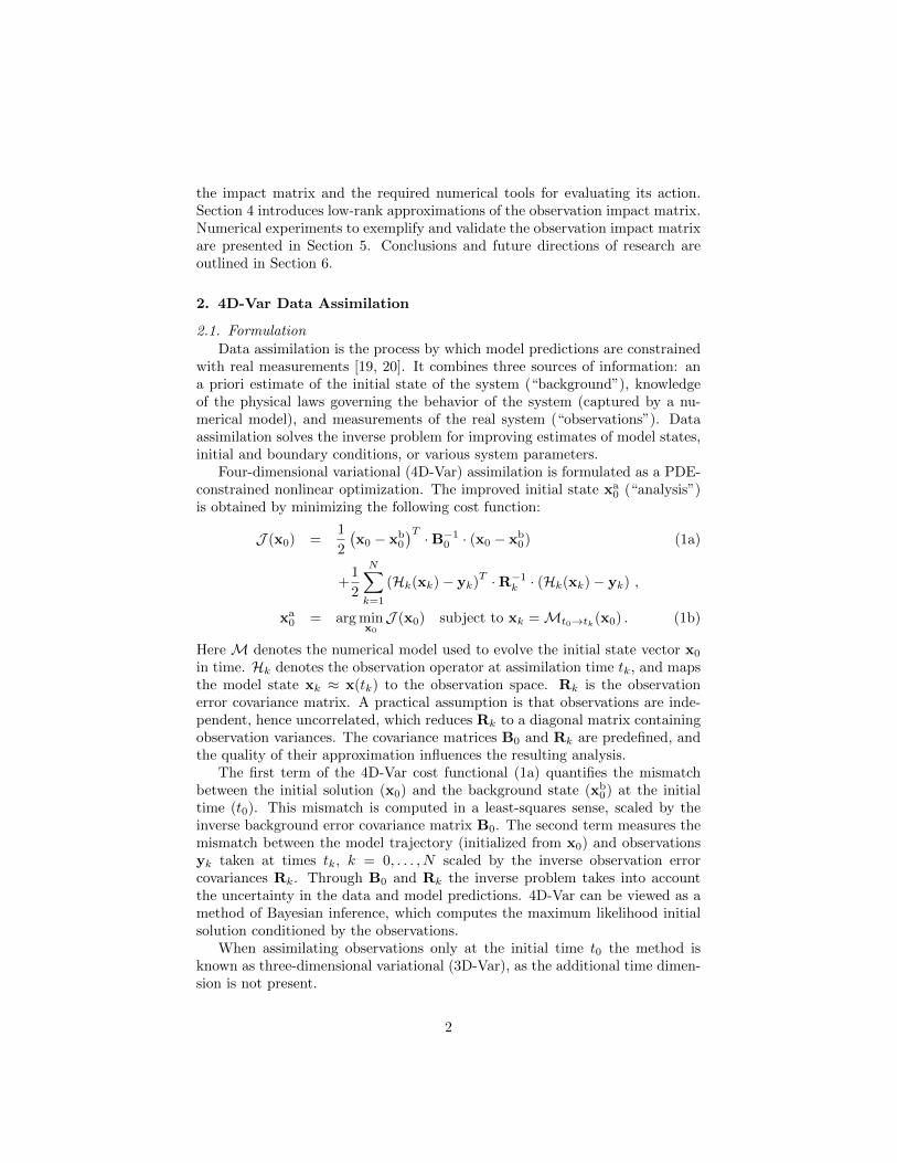
Algorithm 1 Iterative algorithm for low-rank approximations

1: Solve iteratively the eigenvalue problem for the 4D-Var Hessian (14)2: Map newly generated eigenvectors through the tangent linear model (15)3: Compute the truncated SVD of the resulting matrix (16)4: Project the left singular vectors onto the eigenvector base of the 4D-Var

Hessian and build the low-rank approximation of T (17)

4.2. An ensemble-based (parallel) approach for matrix-free low-rank approxima-tions

This approach uses a “randomized SVD” algorithm [31] to compute theMoore-Penrose pseudoinverse [32] of the Hessian. The 4D-Var Hessian matrixA−10 is available only in operator form, i.e., only matrix vector products can beevaluated by running the second order adjoint. The randomized algorithm is asfollows:

1: Draw p random vectors and form a matrix Ω.2: Compute the product Y = A−10 Ω using Hessian-vector multiplications, i.e.,

running the second order order adjoint model for each column.3: Construct the QR decomposition Y = QR.

Each of the above steps can be performed in parallel.The columns of Q form an orthonormal basis for the range of Y. Randomized

SVD uses a series of algebraic manipulations, starting from the observation thatQ is also the orthonormal factor in the QR decomposition of A−10 :

A−10 = Q B , B = Q∗A−10 , B∗ = A−10 Q . (18)

Next, compute an SVD of B:

B = UB ΣB V∗B (19)

and replace (19) in (18) to obtain the SVD of A−10 :

A−10 = Q UB ΣB V∗B = UA ΣB V∗B . (20)

The left singular vectors of A represent the projections of the left singularvectors of B onto the columns of Q. The singular values and right singularvectors of A are the same as those of B. The pseudoinverse of the 4D-VarHessian A−10 reads:

A+0 ≈ VB Σ+

B U∗A . (21)

The observation impact matrix is approximated using the tangent linearmodel M0,k and the pseudoinverse A+

0 :

T ≈N∑

k=1

M0,k A+0 . (22)

The computational flow is summarized in Algorithm 2.

9

Algorithm 2 Sampling algorithm for low-rank approximations

1: Build the matrix B, through parallel second-adjoint runs (18)2: Compute a full SVD of B (19)3: Project the left singular vectors of B in Q and form the SVD of A−10 (20)4: Compute the Hessian pseudoinverse A+

0 (21)5: Build the impact matrix T through parallel tangent linear runs (22)

Computing the rows of B (18) is done as matrix-vector products throughsecond-order adjoint runs that can be performed in parallel. The last step,which propagates the components of the pseudoinverse through the linearizationof the model, is achieved by multiple tangent linear model runs in parallel. Thetangent model results are checkpointed at each of the observation times, so thatonly one run across the entire time horizon is necessary for each input vector.

5. Applications

We illustrate several applications of the observation impact matrix in 4D-Var using the two-dimensional shallow water equations. We first describe thesystem and its numerical discretization, then present the 4D-Var implementa-tion and the experimental setting for data assimilation. Observation sensitivityis computed both in full and using low-rank approximation to assess how wellthe latter captures the essential features. We apply this analysis to three ap-plications, namely, detecting the change in impact from perfect data to noisydata, pruning the least important observations, and detecting faulty sensors.

5.1. Test problem: shallow water equations

The two-dimensional shallow-water equations (2D swe) [33] approximatethe movement of a thin layer of fluid inside a basin:

∂

∂th+

∂

∂x(uh) +

∂

∂y(vh) = 0

∂

∂t(uh) +

∂

∂x

(u2h+

1

2gh2)

+∂

∂y(uvh) = 0 (23)

∂

∂t(vh) +

∂

∂x(uvh) +

∂

∂y

(v2h+

1

2gh2)

= 0 .

Here h(t, x, y) is the fluid layer thickness, and u(t, x, y) and v(t, x, y) are thecomponents of the velocity field of the fluid. The gravitational acceleration isdenoted by g.

We consider a spatial domain Ω = [−3, 3]2 (spatial units), and an integra-tion window is t0 = 0 ≤ t ≤ tf = 0.1 (time units). Boundary conditions areconsidered periodic. The space discretization is realized using a finite volumescheme, and the time integration uses a fourth Runge-Kutta scheme, following

10

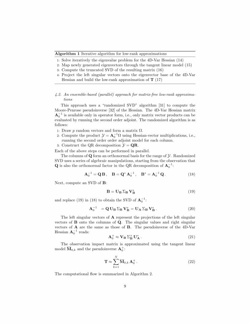
Table 1: Normalized CPU times of different sensitivity models. The forwardmodel takes one time unit to run.

fwd 1tlm 2.5 fwd + tlm 3.5foa 3.7 fwd + foa 4.7soa 12.8 fwd + tlm + foa + soa 20

the method Lax-Wendroff [34]. The model uses a square -q × q uniform spa-tial discretization grid, which brings the number of model (state) variables ton = 3 q2.

We use the automatic differentiation tool TAMC [35, 36] to build varioussensitivity models, as follows. The tangent-linear model (tlm) propagates per-turbations forward in time. The first-order adjoint model (foa) propagatesperturbations backwards in time, and efficiently computes the gradient of ascalar cost functional defined on the model states. The second-order adjointmodel (soa) computes the product between the Hessian of the cost functionand a user-defined vector [22].

The overhead introduced by the sensitivity models is considerable. Table 1presents the CPU times of tlm, foa, and soa models (normalized with respectto that of one fwd run). One soa integration is about 3.5 times more expensivethan a single first-order adjoint run, while the foa takes 3.7 times longer thanthe forward run. These relative costs depend on the discretization methodologyand the implementation of sensitivities. Our previous research showed how tobuild efficient adjoint models by reusing computations performed in the forwardrun [22]. For example, for the shallow water model, the alternative continuousadjoints we built required a fraction of the forward model CPU time to run.

5.2. Data assimilation setup

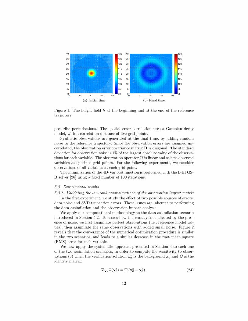
The 4D-Var system is set up for a simple version of the “circular dam”problem [37]. The reference initial height field h is a Gaussian bell of a widthequal to 1 length units centered on the grid, and the reference initial velocityvector components are constant u = v = 0. The physical interpretation is thatthe front of water falls to the ground (h decreases) under the effect of gravityand creates concentric ripples which propagate towards the boundaries. Figures1 represent snapshots of the reference trajectory at initial and final time.

The computational grid is square and regular with q = 40 grid points ineach direction, for a total of 4800 model variables (states). The simulation timeinterval is set to 0.01 seconds, using N = 100 timesteps of size 0.0001 (timeunits).

The h component of the a priori estimate (background) xb is generated byadding a correlated perturbation to the h reference solution at initial time. Thebackground error covariance B0 corresponds to a standard deviation of 5% ofthe reference field values. For the u and v components we use white noise to

11

0 10 20 30 400

5

10

15

20

25

30

35

40

90

95

100

105

110

115

120

125

130

(a) Initial time

0 10 20 30 400

5

10

15

20

25

30

35

40

90

95

100

105

110

115

120

125

130

(b) Final time

Figure 1: The height field h at the beginning and at the end of the referencetrajectory.

prescribe perturbations. The spatial error correlation uses a Gaussian decaymodel, with a correlation distance of five grid points.

Synthetic observations are generated at the final time, by adding randomnoise to the reference trajectory. Since the observation errors are assumed un-correlated, the observation error covariance matrix R is diagonal. The standarddeviation for observation noise is 1% of the largest absolute value of the observa-tions for each variable. The observation operatorH is linear and selects observedvariables at specified grid points. For the following experiments, we considerobservations of all variables at each grid point.

The minimization of the 4D-Var cost function is performed with the L-BFGS-B solver [26] using a fixed number of 100 iterations.

5.3. Experimental results

5.3.1. Validating the low-rank approximations of the observation impact matrix

In the first experiment, we study the effect of two possible sources of errors:data noise and SVD truncation errors. These issues are inherent to performingthe data assimilation and the observation impact analysis.

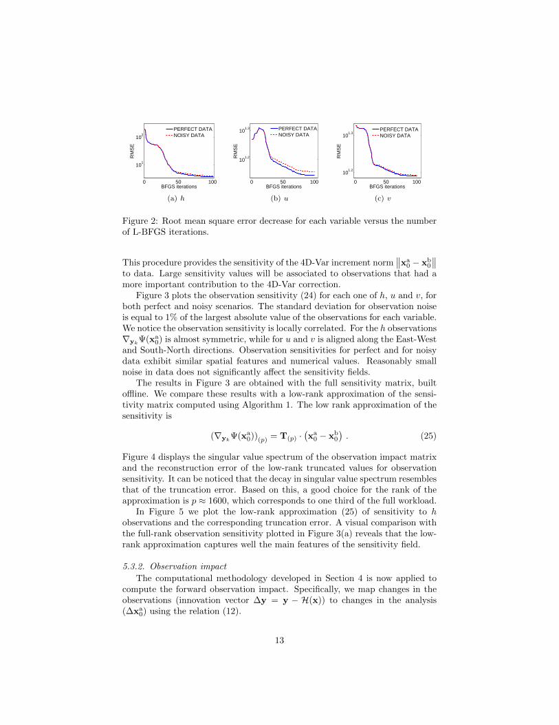
We apply our computational methodology to the data assimilation scenariointroduced in Section 5.2. To assess how the reanalysis is affected by the pres-ence of noise, we first assimilate perfect observations (i.e., reference model val-ues), then assimilate the same observations with added small noise. Figure 2reveals that the convergence of the numerical optimization procedure is similarin the two scenarios, and leads to a similar decrease in the root mean square(RMS) error for each variable.

We now apply the systematic approach presented in Section 4 to each oneof the two assimilation scenarios, in order to compute the sensitivity to obser-vations (8) when the verification solution xv

0 is the background xb0 and C is the

identity matrix:

∇ykΨ(xa

0) = T (xa0 − xb

0) . (24)

12

0 50 100

101

102

BFGS iterations

RM

SE

PERFECT DATANOISY DATA

(a) h

0 50 100

101.2

101.3

BFGS iterations

RM

SE

PERFECT DATANOISY DATA

(b) u

0 50 100

101.2

101.3

BFGS iterations

RM

SE

PERFECT DATANOISY DATA

(c) v

Figure 2: Root mean square error decrease for each variable versus the numberof L-BFGS iterations.

This procedure provides the sensitivity of the 4D-Var increment norm∥∥xa

0 − xb0

∥∥to data. Large sensitivity values will be associated to observations that had amore important contribution to the 4D-Var correction.

Figure 3 plots the observation sensitivity (24) for each one of h, u and v, forboth perfect and noisy scenarios. The standard deviation for observation noiseis equal to 1% of the largest absolute value of the observations for each variable.We notice the observation sensitivity is locally correlated. For the h observations∇yk

Ψ(xa0) is almost symmetric, while for u and v is aligned along the East-West

and South-North directions. Observation sensitivities for perfect and for noisydata exhibit similar spatial features and numerical values. Reasonably smallnoise in data does not significantly affect the sensitivity fields.

The results in Figure 3 are obtained with the full sensitivity matrix, builtoffline. We compare these results with a low-rank approximation of the sensi-tivity matrix computed using Algorithm 1. The low rank approximation of thesensitivity is

(∇ykΨ(xa

0))(p) = T(p) ·(xa0 − xb

0

). (25)

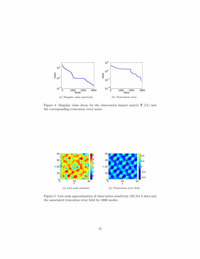
Figure 4 displays the singular value spectrum of the observation impact matrixand the reconstruction error of the low-rank truncated values for observationsensitivity. It can be noticed that the decay in singular value spectrum resemblesthat of the truncation error. Based on this, a good choice for the rank of theapproximation is p ≈ 1600, which corresponds to one third of the full workload.

In Figure 5 we plot the low-rank approximation (25) of sensitivity to hobservations and the corresponding truncation error. A visual comparison withthe full-rank observation sensitivity plotted in Figure 3(a) reveals that the low-rank approximation captures well the main features of the sensitivity field.

5.3.2. Observation impact

The computational methodology developed in Section 4 is now applied tocompute the forward observation impact. Specifically, we map changes in theobservations (innovation vector ∆y = y − H(x)) to changes in the analysis(∆xa

0) using the relation (12).

13

0 20 400

10

20

30

40

x

y

0

1

2

3

4

5

(a) perfect h observations

0 20 400

10

20

30

40

x

y

0

2

4

(b) noisy h observations

0 20 400

10

20

30

40

x

y

−1

−0.5

0

0.5

1

(c) perfect u observations

0 20 400

10

20

30

40

x

y

−1

−0.5

0

0.5

1

(d) noisy u observations

0 20 400

10

20

30

40

x

y

−1

0

1

(e) perfect v observations

0 20 400

10

20

30

40

x

y

−1

0

1

(f) noisy v observations

Figure 3: Sensitivity field (24) for perfect and for noisy observations of h, u,and v.

14

0 1600 3200 480010

−2

100

102

Mode

Val

ue

(a) Singular value spectrum

0 1600 3200 480010

−10

10−5

100

105

Rank

RM

S

(b) Truncation error

Figure 4: Singular value decay for the observation impact matrix T (11) andthe corresponding truncation error norm.

0 20 400

10

20

30

40

x

y

0

1

2

3

4

5

(a) Low-rank estimate

0 20 400

10

20

30

40

x

y

−0.4

−0.2

0

0.2

0.4

(b) Truncation error field

Figure 5: Low-rank approximation of observation sensitivity (25) for h data andthe associated truncation error field for 1600 modes.

15

0 20 400

10

20

30

40

x

y

−0.5

0

0.5

(a) Full-rank impact for center obser-vation

0 20 400

10

20

30

40

x

y

−0.5

0

0.5

(b) Low-rank impact for center obser-vation

0 20 400

10

20

30

40

x

y

−0.05

0

0.05

(c) Full-rank impact for corner obser-vation

0 20 400

10

20

30

40

x

y

−0.05

0

0.05

(d) Low-rank impact for corner obser-vation

Figure 6: The impact of two h observations from assimilation time t100, placedin the center and in the corner of the grid. Both full rank and reduced ranksolutions are shown. 500 modes are used for the reduced rank approximation.

We compute the observation impact in full-rank and low-rank correspondingto two observations of h, one in the center (grid coordinates (20, 20)) and one inthe corner (at (5, 5)) at the locations represented with white markers. This isachieved by multiplying TT with a vector containing just the innovation broughtby the observation whose impact we want to evaluate (all other vector entrieshave value zero). The resulting impact fields are plot in Figure 6. The spatialfeatures of the observation impact have a local radial correlation in both cases.This means the information carried by the observation is spread in its proximityby the 4D-Var process; this is also true across the periodic boundaries of theshallow water system. Moreover, the low-rank approximations are able to pickup the important features of the full-rank calculations, and provide impacts ofa similar magnitude.

Having already computed the SVD of the observation impact matrix, we alsolook at the directions in the data space ∆y that have the largest impact on theanalysis, and the directions in the 4D-Var correction space ∆x that benefit mostfrom the assimilation. These directions are given by the dominant left and rightsingular vectors of TT , respectively. Figure 7 plots the first dominant left (and

16

0 20 400

10

20

30

40

x

y

−2000

−1000

0

1000

(a) First dominant left singular vector(model space)

0 20 400

10

20

30

40

x

y

−2

0

2

x 108

(b) First 500 dominant left singularvectors (model space)

0 20 400

10

20

30

40

x

y

−10

0

10

(c) First dominant right singular vector(observation space)

0 20 400

10

20

30

40

x

y

−2

−1

0

1

2

3

x 106

(d) First 500 dominant right singularvectors (observation space)

Figure 7: Principal directions of growth in observation and solution space, asdefined by the dominant left and right singular vectors of the observation impactmatrix.

right) singular vectors corresponding to the h variable, and also the compositionof the most important 500 directions for the observation and solution space usingthe formula

vdomin =

500∑i=1

s2i ∗ vi , (26)

where si and vi are the singular pair corresponding to the i-th mode.

5.3.3. Pruning observations based on sensitivity values

In this experiment we illustrate how sensitivity analysis can be used to selectthe most useful data points.

For this, we compute the 4D-Var reanalysis and then apply the observationimpact methodology to compute the sensitivity of the cost function Ψ to eachone of the 4800 observations (24). We then split our observation set in threesubsets of 1600 observations, corresponding to each one of h, u and v. Withineach subset, we order the observations by their sensitivity; the top 800 obser-vations form the high sensitivity set, and the ones in the bottom 800 form the

17

1 10 100

10

100

BFGS iterations [log scale]

RM

SE

[log

sca

le]

FULLHIGHLOW

(a) h RMS error decrease versus thenumber of L-BFGS iterations.

1 10 100

101.2

101.3

BFGS iterations [log scale]

RM

SE

[log

sca

le]

FULLHIGHLOW

(b) u RMS error decrease versus thenumber of L-BFGS iterations.

1 10 100

101.2

101.3

BFGS iterations [log scale]

RM

SE

[log

sca

le]

FULLHIGHLOW

(c) v RMS error decrease versus thenumber of L-BFGS iterations.

0 10 20 30 400

10

20

30

40

x

y

(d) Location of high (red) and low im-pact observations

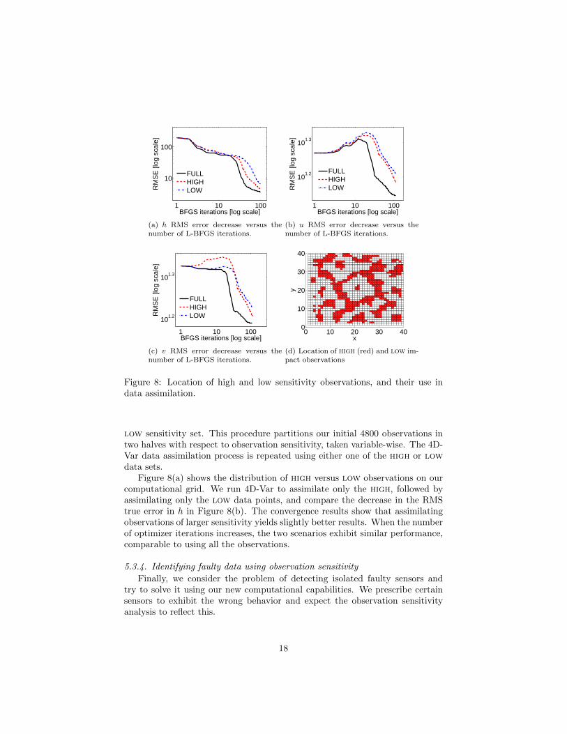
Figure 8: Location of high and low sensitivity observations, and their use indata assimilation.

low sensitivity set. This procedure partitions our initial 4800 observations intwo halves with respect to observation sensitivity, taken variable-wise. The 4D-Var data assimilation process is repeated using either one of the high or lowdata sets.

Figure 8(a) shows the distribution of high versus low observations on ourcomputational grid. We run 4D-Var to assimilate only the high, followed byassimilating only the low data points, and compare the decrease in the RMStrue error in h in Figure 8(b). The convergence results show that assimilatingobservations of larger sensitivity yields slightly better results. When the numberof optimizer iterations increases, the two scenarios exhibit similar performance,comparable to using all the observations.

5.3.4. Identifying faulty data using observation sensitivity

Finally, we consider the problem of detecting isolated faulty sensors andtry to solve it using our new computational capabilities. We prescribe certainsensors to exhibit the wrong behavior and expect the observation sensitivityanalysis to reflect this.

18

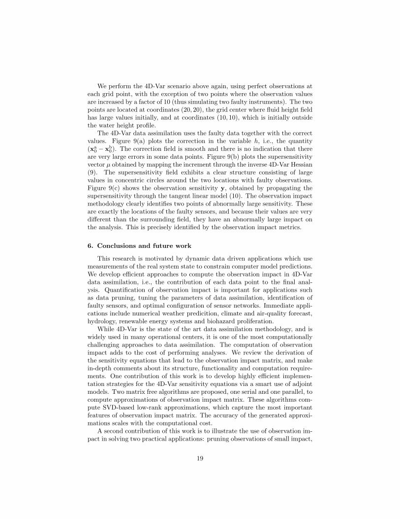
We perform the 4D-Var scenario above again, using perfect observations ateach grid point, with the exception of two points where the observation valuesare increased by a factor of 10 (thus simulating two faulty instruments). The twopoints are located at coordinates (20, 20), the grid center where fluid height fieldhas large values initially, and at coordinates (10, 10), which is initially outsidethe water height profile.

The 4D-Var data assimilation uses the faulty data together with the correctvalues. Figure 9(a) plots the correction in the variable h, i.e., the quantity(xa

0 − xb0). The correction field is smooth and there is no indication that there

are very large errors in some data points. Figure 9(b) plots the supersensitivityvector µ obtained by mapping the increment through the inverse 4D-Var Hessian(9). The supersensitivity field exhibits a clear structure consisting of largevalues in concentric circles around the two locations with faulty observations.Figure 9(c) shows the observation sensitivity y, obtained by propagating thesupersensitivity through the tangent linear model (10). The observation impactmethodology clearly identifies two points of abnormally large sensitivity. Theseare exactly the locations of the faulty sensors, and because their values are verydifferent than the surrounding field, they have an abnormally large impact onthe analysis. This is precisely identified by the observation impact metrics.

6. Conclusions and future work

This research is motivated by dynamic data driven applications which usemeasurements of the real system state to constrain computer model predictions.We develop efficient approaches to compute the observation impact in 4D-Vardata assimilation, i.e., the contribution of each data point to the final anal-ysis. Quantification of observation impact is important for applications suchas data pruning, tuning the parameters of data assimilation, identification offaulty sensors, and optimal configuration of sensor networks. Immediate appli-cations include numerical weather predicition, climate and air-quality forecast,hydrology, renewable energy systems and biohazard proliferation.

While 4D-Var is the state of the art data assimilation methodology, and iswidely used in many operational centers, it is one of the most computationallychallenging approaches to data assimilation. The computation of observationimpact adds to the cost of performing analyses. We review the derivation ofthe sensitivity equations that lead to the observation impact matrix, and makein-depth comments about its structure, functionality and computation require-ments. One contribution of this work is to develop highly efficient implemen-tation strategies for the 4D-Var sensitivity equations via a smart use of adjointmodels. Two matrix free algorithms are proposed, one serial and one parallel, tocompute approximations of observation impact matrix. These algorithms com-pute SVD-based low-rank approximations, which capture the most importantfeatures of observation impact matrix. The accuracy of the generated approxi-mations scales with the computational cost.

A second contribution of this work is to illustrate the use of observation im-pact in solving two practical applications: pruning observations of small impact,

19

0 20 400

10

20

30

40

x

y

−10

−5

0

5

10

(a) 4D-Var increment

0 20 400

10

20

30

40

x

y−10

0

10

(b) Supersensitivity field

0 10 20 30 400

5

10

15

20

25

30

35

40

−50

−40

−30

−20

−10

0

(c) Sensitivity to observations

Figure 9: Observation sensitivity field when the assimilated data is corrupted attwo locations with coordinates (10,10) and (20,20). The location of the faultysensors is unknown to the data assimilation system, but is retrieved via theobservation impact methodology.

20

and detecting faulty sensors. Numerical experiments that validate the proposedcomputational framework are carried out with a two dimensional shallow waterequations system.

Several future research directions emerge from this study. On the computa-tional side, the impact approximation algorithms can be further developed toachieve superior performance. A rigorous analysis of approximation errors willbe developed to guide the choice of the number of iterations and the truncationlevel. On the application side, our will be integrated in real large scale applica-tions to provide a measure of importance of different measurements in real timeassimilation. In hindsight, the impact can be used to prune the data subsets andto detect erroneous data points. In foresight, it can be used to design efficientstrategies of sensor placement for targeted and adaptive observations.

Acknowledgements

This work was supported by the National Science Foundation through theawards NSF DMS-0915047, NSF CCF-0635194, NSF CCF-0916493 and NSFOCI-0904397, and by AFOSR DDDAS program through the awards FA9550–12–1–0293–DEF and AFOSR 12-2640-06.

References

[1] T. Palmer, T. Gelaro, J. Barkmeijer, and R. Buizza. Singular vectors,metrics, and adaptive observations. Journal of the Atmospheric Sciences,55(4):633–653, 1998.

[2] W. Liao, A. Sandu, and G. Carmichael. Total energy singular vector anal-ysis for atmospheric chemical transport models. Monthly Weather Review,134(9):2443–2465, 2006.

[3] D. Zupanski, A.Y. Hou, S.Q. Zhang, M. Zupanski, C.D. Kummerow, andS.H. Cheung. Applications of information theory in ensemble data assimila-tion. Quarterly Journal of the Royal Meteorological Society, 133(627):1533–1545, 2007.

[4] K. Singh, A. Sandu, and M. Jardak. Information theoretic metrics tocharacterize observations in variational data assimilation. Proceedings ofthe International Conference on Computational Science, 9(1):1047–1055,2012.

[5] L.M. Berliner, Z.Q. Lu, and C. Snyder. Statistical design for adaptiveweather observations. Journal of the Atmospheric Sciences, 56(15):2536–2552, 1999.

[6] W. Kang and L. Xu. Optimal placement of mobile sensors for data assim-ilations. Tellus A, 64(0), 2012.

21

[7] R. Gelaro, Y. Zhu, and R.M. Errico. Examination of various-order adjoint-based approximations of observation impact. Meteorologische Zeitschrift,16(6):685–692, 2007.

[8] R. Gelaro and Y. Zhu. Examination of observation impacts derived fromobserving system experiments (OSEs) and adjoint models. Tellus A,61(2):179–193, 2009.

[9] Y. Tremolet. Computation of observation sensitivity and observation im-pact in incremental variational data assimilation. Tellus A, 60(5):964–978,2008.

[10] F.X. Le Dimet and H.E. Ngodock. Sensitivity analysis in variational dataassimilation. Journal of the Meteorological Society of Japan, 75(1):245–255,1997.

[11] D.N. Daescu. On the sensitivity equations of four-dimensional variational(4D-Var) data assimilation. Monthly Weather Review, 136(8):3050–3065,2008.

[12] D.N. Daescu and R. Todling. Adjoint sensitivity of the model forecast todata assimilation system error covariance parameters. Quarterly Journalof the Royal Meteorological Society, 136(653):2000–2012, 2010.

[13] D.G. Cacuci. Sensitivity theory for nonlinear systems. I: Nonlinear func-tional analysis approach. Journal of Mathematical Physics, 22:2794, 1981.

[14] Z. Wang, I.M. Navon, F.X. Le Dimet, and X. Zou. The second order adjointanalysis: theory and applications. Meteorology and Atmospheric Physics,50(3):3–20, 1992.

[15] A. Sandu and L. Zhang. Discrete second order adjoints in atmo-spheric chemical transport modeling. Journal of Computational Physics,227(12):5949–5983, 2008.

[16] J. Ye. Generalized low rank approximations of matrices. Machine Learning,61(1-3):167–191, 2005.

[17] M.W. Berry and R.D. Fierro. Low-rank orthogonal decompositions forinformation retrieval applications. Numerical Linear Algebra with Applica-tions, 3(4):301–327, 1996.

[18] I.S. Dhillon and D.S. Modha. Concept decompositions for large sparse textdata using clustering. Machine Learning, 42(1-2):143–175, 2001.

[19] R. Daley. Atmospheric data analysis. Cambridge University Press, Cam-bridge, 1991.

[20] E. Kalnay. Atmospheric modeling, data assimilation and predictability.Cambridge University Press, Cambridge, 2002.

22

[21] A. Sandu, D.N. Daescu, G.R. Carmichael, and T. Chai. Adjoint sensitivityanalysis of regional air quality models. Journal of Computational Physics,204(1):222–252, 2005.

[22] A. Cioaca, A. Sandu, and M. Alexe. Second-order adjoints for solving PDE-constrained optimization problems. Optimization Methods and Software,27(4-5):625–653, 2011.

[23] A. Griewank. On automatic differentiation. Mathematical Programming:recent developments and applications, 6:83–107, 1989-.

[24] I.Y. Gejadze, F.X. Le Dimet, and V. Shutyaev. On analysis error covari-ances in variational data assimilation. SIAM Journal on Scientific Com-puting, 30(4):1847–1874, 2008.

[25] A. Cioaca, A. Sandu, and E. de Sturler. Efficient methods for computingobservation impact in 4d-var data assimilation. Technical report, 2012.

[26] C. Zhu, R.H. Byrd, P. Lu, and J. Nocedal. Algorithm 778: L-BFGS-B:Fortran subroutines for large-scale bound-constrained optimization. ACMTransactions on Mathematical Software (TOMS), 23(4):550–560, 1997.

[27] C. Lanczos. An iteration method for the solution of the eigenvalue problemof linear differential and integral operators. United States GovernmentPress Office, 1950.

[28] W.E. Arnoldi. The principle of minimized iterations in the solution of thematrix eigenvalue problem. Quarterly of Applied Mathematics, 9(1):17–29,1951.

[29] G.L.G. Sleijpen and H.A. Van der Vorst. A Jacobi–Davidson iterationmethod for linear eigenvalue problems. SIAM Review, 42(2):267–293, 2000.

[30] D.R. Fokkema and M.B. van Gijzen. Short manual for the JDQZ-package,1999.

[31] E. Liberty, F. Woolfe, P.G. Martinsson, V. Rokhlin, and M. Tygert. Ran-domized algorithms for the low-rank approximation of matrices. Proceed-ings of the National Academy of Sciences, 104(51):20167–20172, 2007.

[32] T.O. Lewis and T.G. Newman. Pseudoinverss of postive semidefeinite ma-trices. SIAM Journal on Applied Mathematics, 16(4):701–703, 1968.

[33] D.D. Houghton and A. Kasahara. Nonlinear shallow fluid flow over anisolated ridge. Communications on Pure and Applied Mathematics, 21(1):1–23, 1968.

[34] R. Liska and B. Wendroff. Composite schemes for conservation laws. SIAMJournal of Numerical Analysis, 35(6):2250–2271, 1998.

23

[35] R. Giering. Tangent linear and adjoint model compiler. User Manual,TAMC Version, 4, 1997.

[36] R. Giering and T. Kaminski. Recipes for adjoint code construction. ACMTransactions on Mathematical Software, 24(4):437–474, 1998.

[37] K. Anastasiou and C.T. Chan. Solution of the 2d shallow water equa-tions using the finite volume method on unstructured triangular meshes.International Journal for Numerical Methods in Fluids, 24(11):1225–1245,1997.

24