computational number theory in relation with l-functions

HAL Id: hal-01883052https://hal.inria.fr/hal-01883052

Submitted on 27 Sep 2018

HAL is a multi-disciplinary open accessarchive for the deposit and dissemination of sci-entific research documents, whether they are pub-lished or not. The documents may come fromteaching and research institutions in France orabroad, or from public or private research centers.

L’archive ouverte pluridisciplinaire HAL, estdestinée au dépôt et à la diffusion de documentsscientifiques de niveau recherche, publiés ou non,émanant des établissements d’enseignement et derecherche français ou étrangers, des laboratoirespublics ou privés.

Computational Number Theory in Relation withL-Functions

Henri Cohen

To cite this version:Henri Cohen. Computational Number Theory in Relation with L-Functions. Ilker Inam; EnginBüyükaşık. Notes from the International School on Computational Number Theory, Birkhäuser,pp.171-266, 2019, Tutorials, Schools, and Workshops in the Mathematical Sciences, �10.1007/978-3-030-12558-5_3�. �hal-01883052�

https://hal.inria.fr/hal-01883052

https://hal.archives-ouvertes.fr

Computational Number Theory in Relation withL-Functions

Henri Cohen

Abstract We give a number of theoretical and practical methods related to the com-

putation of L-functions, both in the local case (counting points on varieties over

finite fields, involving in particular a detailed study of Gauss and Jacobi sums),

and in the global case (for instance Dirichlet L-functions, involving in particular

the study of inverse Mellin transforms); we also give a number of little-known but

very useful numerical methods, usually but not always related to the computation of

L-functions.

1 L-Functions

This course is divided into five parts. In the first part (Sections 1 and 2), we introduce

the notion of L-function, give a number of results and conjectures concerning them,

and explain some of the computational problems in this theory. In the second part

(Sections 3 to 6), we give a number of computational methods for obtaining the

Dirichlet series coefficients of the L-function, so is arithmetic in nature. In the third

part (Section 7), we give a number of analytic tools necessary for working with L-

functions. In the fourth part (Sections 8 and 9), we give a number of very useful

numerical methods which are not sufficiently well-known, most of which being also

related to the computation of L-functions. The fifth part (Sections 10 and 11) gives

the Pari/GP commands corresponding to most of the algorithms and examples

given in the course. A final Section 12 gives as an appendix some basic definitions

and results used in the course which may be less familiar to the reader.

Universite de Bordeaux, CNRS, INRIA, IMB, UMR 5251, F-33400 Talence, France, e-mail:

[email protected]

1

2 Henri Cohen

1.1 Introduction

The theory of L-functions is one of the most exciting subjects in number theory. It

includes for instance two of the crowning achievements of twentieth century math-

ematics, first the proof of the Weil conjectures and of the Ramanujan conjecture

by Deligne in the early 1970’s, using the extensive development of modern alge-

braic geometry initiated by Weil himself and pursued by Grothendieck and follow-

ers in the famous EGA and SGA treatises, and second the proof of the Shimura–

Taniyama–Weil conjecture by Wiles et al., implying among other things the proof

of Fermat’s last theorem. It also includes two of the seven 1 million dollar Clay

problems for the twenty-first century, first the Riemann hypothesis, and second the

Birch–Swinnerton-Dyer conjecture which in my opinion is the most beautiful, if not

the most important, conjecture in number theory, or even in the whole of mathemat-

ics, together with similar conjectures such as the Beilinson–Bloch conjecture.

There are two kinds of L-functions: local L-functions and global L-functions.

Since the proof of the Weil conjectures, local L-functions are rather well understood

from a theoretical standpoint, but somewhat less from a computational standpoint.

Much less is known on global L-functions, even theoretically, so here the compu-

tational standpoint is much more important since it may give some insight on the

theoretical side.

Before giving a definition of L-functions, we look in some detail at a large num-

ber of special cases of global L-functions.

1.2 The Prototype: the Riemann Zeta Function ζ (s)

The simplest of all (global) L-function is the Riemann zeta function ζ (s) defined by

ζ (s) = ∑n≥1

1

ns.

This is an example of a Dirichlet series (more generally ∑n≥1 a(n)/ns, or even more

generally ∑n≥1 1/λ sn , but we will not consider the latter). As such, it has a half-plane

of absolute convergence, here ℜ(s)> 1.

The properties of this function, studied initially by Bernoulli and Euler, are as

follows, given historically:

1. (Bernoulli, Euler): it has special values. When s = 2, 4,... is a strictly positive

even integer, ζ (s) is equal to π s times a rational number. π is here a period,

and is of course the usual π used for measuring circles. These rational numbers

have elementary generating functions, and are equal up to easy terms to the so-

called Bernoulli numbers. For example ζ (2) = π2/6, ζ (4) = π4/90, etc. This

was conjectured by Bernoulli and proved by Euler. Note that the proof in 1735

of the so-called Basel problem:

Computational Number Theory in Relation with L-Functions 3

ζ (2) = 1+1

22+

1

32+

1

42+ · · ·= π2

6

is one of the crowning achievements of mathematics of that time.

2. (Euler): it has an Euler product: for ℜ(s)> 1 one has the identity

ζ (s) = ∏p∈P

1

1− 1/ps,

where P is the set of prime numbers. This is exactly equivalent to the so-called

fundamental theorem of arithmetic. Note in passing (this does not seem interest-

ing here but will be important later) that if we consider 1−1/ps as a polynomial

in 1/ps = T , its reciprocal roots all have the same modulus, here 1, this being of

course trivial.

3. (Riemann, but already “guessed” by Euler in special cases): it has an analytic

continuation to a meromorphic function in the whole complex plane, with a sin-

gle pole, at s = 1, with residue 1, and a functional equation Λ(1− s) = Λ(s),where Λ(s) = ΓR(s)ζ (s), with ΓR(s) = π−s/2Γ (s/2), and Γ is the gamma func-

tion (see appendix).

4. As a consequence of the functional equation, we have ζ (s) = 0 when s = −2,

−4,..., ζ (0) =−1/2, but we also have special values at s =−1, s =−3,... which

are symmetrical to those at s = 2, 4,... (for instance ζ (−1) = −1/12, ζ (−3) =1/120, etc.). This is the part which was guessed by Euler.

Roughly speaking, one can say that a global L-function is a function having prop-

erties similar to all the above. We will of course be completely precise below. Two

things should be added immediately: first, the existence of special values will not

be part of the definition but, at least conjecturally, a consequence. Second, all the

global L-functions that we will consider should conjecturally satisfy a Riemann hy-

pothesis: when suitably normalized, and excluding “trivial” zeros, all the zeros of

the function should be on the line ℜ(s) = 1/2, axis of symmetry of the functional

equation. Note that even for the simplest L-function, ζ (s), this is not proved.

1.3 Dedekind Zeta Functions

The Riemann zeta function is perhaps too simple an example to get the correct

feeling about global L-functions, so we generalize:

Let K be a number field (a finite extension of Q) of degree d. We can define its

Dedekind zeta function ζK(s) for ℜ(s)> 1 by

ζK(s) =∑a

1

N (a)s= ∑

n≥1

i(n)

ns,

4 Henri Cohen

where a ranges over all (nonzero) integral ideals of the ring of integers ZK of K,

N (a) = [ZK : a] is the norm of a, and i(n) denotes the number of integral ideals of

norm n.

This function has very similar properties to those of ζ (s) (which is the special

case K =Q). We give them in a more logical order:

1. It can be analytically continued to the whole complex plane into a meromorphic

function having a single pole, at s= 1, with known residue, and it has a functional

equation ΛK(1− s) = ΛK(s), where

ΛK(s) = |DK |s/2ΓR(s)r1+r2ΓR(s+ 1)r2 ,

where (r1,2r2) are the number of real and complex embeddings of K and DK its

discriminant.

2. It has an Euler product ζK(s) = ∏p 1/(1−1/N (p)s), where the product is over

all prime ideals of ZK . Note that this can also be written

ζK(s) = ∏p∈P

∏p|p

1

1− 1/p f (p/p)s,

where f (p/p) = [ZK/p :Z/pZ] is the so-called residual index of p above p. Once

again, note that if we set as usual 1/ps = T , the reciprocal roots of 1−T f (p/p)

all have modulus 1.

3. It has special values, but only when K is a totally real number field (r2 = 0,

r1 = d): in that case ζK(s) is a rational number if s is a negative odd integer, or

equivalently by the functional equation, it is a rational multiple of√|DK |πds if s

is a positive even integer.

An important new phenomenon occurs: recall that ∑p|p e(p/p) f (p/p)= d, where

e(p/p) is the so-called ramification index, which is equivalent to the defining equal-

ity pZK = ∏p|p pe(p/p). In particular ∑p|p f (p/p) = d if and only if e(p/p) = 1 for

all p, which means that p is unramified in K/Q; one can prove that this is equivalent

to p ∤ DK . Thus, the local L-function LK,p(T ) = ∏p|p(1−T f (p/p)) has degree in T

exactly equal to d for all but a finite number of primes p, which are exactly those

which divide the discriminant DK , and for those “bad” primes the degree is strictly

less than d. In addition, note that the number of ΓR factors in the completed function

ΛK(s) is equal to r1 + 2r2, hence once again equal to d.

Examples:

1. Let D be the discriminant of a quadratic field, and let K = Q(√

D). In that

case, ζK(s) factors as ζK(s) = ζ (s)L(χD,s), where χD =(

D.

)is the Legendre–

Kronecker symbol, and L(χD,s) = ∑n≥1 χD(n)/ns. Thus, the local L-function at

a prime p is given by

LK,p(T ) = (1−T)(1− χD(p)T ) = 1− apT + χD(p)T 2 ,


with ap = 1+ χD(p). Note that ap is equal to the number of solutions in Fp of

the equation x2 = D.

2. Let us consider two special cases of (1): first K = Q(√

5). Since it is a real

quadratic field, it has special values, for instance

ζK(−1) =1

30, ζK(−3) =

1

60, ζK(2) =

2√

5π4

375, ζK(4) =

4√

5π8

84375.

In addition, note that its gamma factor is 5s/2ΓR(s)2.

Second, consider K =Q(√−23). Since it is not a totally real field, ζK(s) does not

have special values. However, because of the factorization ζK(s) = ζ (s)L(χD,s),we can look separately at the special values of ζ (s), which we have already seen

(negative odd integers and positive even integers), and of L(χD,s). It is easy to

prove that the special values of this latter function occurs at negative even integers

and positive odd integers, which have empty intersection which those of ζ (s) and

explains why ζK(s) itself has none. For instance,

L(χD,−2) =−48 , L(χD,−4) = 6816 , L(χD,3) =96√

23π3

12167.

In addition, note that its gamma factor is

23s/2ΓR(s)ΓR(s+ 1) = 23s/2ΓC(s) ,

where we set by definition

ΓC(s) = ΓR(s)ΓR(s+ 1) = 2 · (2π)−sΓ (s)

by the duplication formula for the gamma function.

3. Let K be the unique cubic field up to isomorphism of discriminant−23, defined

for instance by a root of the equation x3− x− 1 = 0. We have (r1,2r2) = (1,2)and DK = −23. Here, one can prove (it is less trivial) that ζK(s) = ζ (s)L(ρ ,s),where L(ρ ,s) is a holomorphic function. Using both properties of ζK and ζ , this

L-function has the following properties:

• It extends to an entire function on C with a functional equation Λ(ρ ,1− s) =Λ(ρ ,s), with

Λ(ρ ,s) = 23s/2ΓR(s)ΓR(s+ 1)L(ρ ,s) = 23s/2ΓC(s)L(ρ ,s) .

Note that this is the same gamma factor as for Q(√−23). However the func-

tions are fundamentally different, since ζQ(√−23)(s) has a pole at s = 1, while

L(ρ ,s) is an entire function.

• It is immediate to show that if we let Lρ ,p(T ) = LK,p(T )/(1−T) be the local

L function for L(ρ ,s), we have Lρ ,p(T ) = 1− apT + χ−23(p)T 2, with ap = 1

if p = 23, ap = 0 if(−23

p

)=−1, and ap = 1 or 2 if

(−23

p

)= 1.

6 Henri Cohen

Remark 1.1. In all of the above examples, the function ζK(s) is divisible by the

Riemann zeta function ζ (s), i.e., the function ζK(s)/ζ (s) is an entire function. This

is known for some number fields K, but is not known in general, even in degree

d = 5 for instance: it is a consequence of the more precise Artin conjecture on the

holomorphy of Artin L-functions.

1.4 Further Examples in Weight 0

It is now time to give examples not coming from number fields. Define a1(n) by the

formal equality

q ∏n≥1

(1− qn)(1− q23n) = ∑n≥1

a1(n)qn = q− q2− q3 + q6 + q8−·· · ,

and set L1(s) = ∑n≥1 a1(n)/ns. The theory of modular forms (here of the Dedekind

eta function) tells us that L1(s) will satisfy exactly the same properties as L(ρ ,s)with ρ as above.

Define a2(n) by the formal equality

1

2

(

∑(m,n)∈Z×Z

qm2+mn+6n2− q2m2+mn+3n2

)= ∑

n≥1

a2(n)qn ,

and set L2(s) = ∑n≥1 a2(n)/ns. The theory of modular forms (here of theta func-

tions) tells us that L2(s) will satisfy exactly the same properties as L(ρ ,s).And indeed, it is an interesting theorem that

L1(s) = L2(s) = L(ρ ,s) :

The “moral” of this story is the following, which can be made mathematically pre-

cise: if two L-functions are holomorphic, have the same gamma factor (includ-

ing in this case the 23s/2), then (conjecturally in general) they belong to a finite-

dimensional vector space. Thus in particular if this vector space is 1-dimensional

and the L-functions are suitably normalized (usually with a(1) = 1), this implies as

here that they are equal.

1.5 Examples in Weight 1

Although we have not yet defined the notion of weight, let me give two further

examples.

Define a3(n) by the formal equality


q ∏n≥1

(1− qn)2(1− q11n)2 = ∑n≥1

a3(n)qn = q− 2q2− q3 + 2q4+ · · · ,

and set L3(s) = ∑n≥1 a3(n)/ns. The theory of modular forms (again of the Dedekind

eta function) tells us that L3(s) will satisfy the following properties, analogous but

more general than those satisfied by L1(s) = L2(s) = L(ρ ,s):

• It has an analytic continuation to the whole complex plane, and if we set

Λ3(s) = 11s/2ΓR(s)ΓR(s+ 1)L3(s) = 11s/2ΓC(s)L3(s) ,

we have the functional equation Λ3(2− s) = Λ3(s). Note the crucial difference

that here 1− s is replaced by 2− s.

• There exists an Euler product L3(s) = ∏p∈P 1/L3,p(1/ps) similar to the pre-

ceding ones in that L3,p(T ) is for all but a finite number of p a second de-

gree polynomial in T . More precisely, if p = 11 we have L3,p(T ) = 1− T ,

while for p 6= 11 we have L3,p(T ) = 1− apT + pT 2, for some ap such that

|ap| < 2√

p. This is expressed more vividly by saying that for p 6= 11 we have

L3,p(T ) = (1−αpT )(1−βpT ), where the reciprocal roots αp and βp have modu-

lus exactly equal to p1/2. Note again the crucial difference with “weight 0” in that

the coefficient of T 2 is equal to p instead of ±1, hence that |αp| = |βp| = p1/2

instead of 1.

As a second example, consider the equation y2 + y = x3− x2− 10x− 20 (an el-

liptic curve E), and denote by Nq(E) the number of projective points of this curve

over the finite field Fq (it is clear that there is a unique point at infinity, so if you

want Nq(E) is one plus the number of affine points). There is a universal recipe to

construct an L-function out of a variety which we will recall below, but here let us

simplify: for p prime, set ap = p+ 1−Np(E) and

L4(s) = ∏p∈P

1/(1− app−s + χ(p)p1−2s) ,

where χ(p) = 1 for p 6= 11 and χ(11) = 0. It is not difficult to show that L4(s)satisfies exactly the same properties as L3(s) (using for instance the elementary

theory of modular curves), so by the moral explained above, it should not come as

a surprise that in fact L3(s) = L4(s).

1.6 Definition of a Global L-Function

With all these examples at hand, it is quite natural to give the following definition

of an L-function, which is not the most general but will be sufficient for us.

Definition 1.2. Let d be a nonnegative integer. We say that a Dirichlet series

L(s) = ∑n≥1 a(n)n−s with a(1) = 1 is an L-function of degree d and weight 0 if

the following conditions are satisfied:

8 Henri Cohen

1. (Ramanujan bound): we have a(n) = O(nε) for all ε > 0, so that in particular

the Dirichlet series converges absolutely and uniformly in any half plane ℜ(s)≥σ > 1.

2. (Meromorphy and Functional equation): The function L(s) can be extended to

C to a meromorphic function of order 1 (see appendix) having a finite number

of poles; furthermore there exist complex numbers λi with nonnegative real part

and an integer N called the conductor such that if we set

γ(s) = Ns/2 ∏1≤i≤d

ΓR(s+λi) and Λ(s) = γ(s)L(s) ,

we have the functional equation

Λ(s) = ωΛ(1− s)

for some complex number ω , called the root number, which will necessarily be

of modulus 1.

3. (Euler Product): For ℜ(s) > 1 we have an Euler product

L(s) = ∏p∈P

1/Lp(1/ps) with Lp(T ) = ∏1≤ j≤d

(1−αp, jT ) ,

and the reciprocal roots αp, j are called the Satake parameters.

4. (Local Riemann hypothesis): for p ∤ N we have |αp, j|= 1, and for p | N we have

either αp, j = 0 or |αp, j|= p−m/2 for some m such that 1≤ m≤ d.

Remarks 1.3 1. More generally Selberg has defined a more general class of L-

functions which first allows Γ (µis+λi) with µi positive real in the gamma factors

and second allows weaker assumptions on N and the Satake parameters.

2. Note that d is both the number of ΓR factors, and the degree in T of the Euler

factors Lp(T ), at least for p ∤ N, while the degree decreases for the “bad” primes

p which divide N.

3. The Ramanujan bound (1) is easily seen to be a consequence of the conditions

that we have imposed on the Satake parameters: in Selberg’s more general defi-

nition this is not the case.

It is important to generalize this definition in the following trivial way:

Definition 1.4. Let w be a nonnegative integer. A function L(s) is said to be an L-

function of degree d and motivic weight w if L(s+w/2) is an L-function of degree d

and weight 0 as above (with the slight additional technical condition that the nonzero

Satake parameters αp, j for p | N satisfy |αp, j|= p−m/2 with 1≤ m≤ w).

For an L-function of weight w, it is clear that the functional equation is Λ(s) =ωΛ(k− s) with k = w+1, and that the Satake parameters will satisfy |αp, j|= pw/2

for p ∤ N, and for p |N we have either αp, j = 0 or |αp, j|= p(w−m)/2 for some integer

m such that 1≤ m≤ w.


Thus, the first examples that we have given are all of weight 0, and the last two

(which are in fact equal) are of weight 1. For those who know the theory of modular

forms, note that the motivic weight (that we denote by w) is one less than the weight

k of the modular form.

2 Origins of L-Functions

As can already be seen in the above examples, it is possible to construct L-functions

in many different ways. In the present section, we look at three different ways for

constructing L-functions: the first is by the theory of modular forms or more gen-

erally of automorphic forms (of which we have seen a few examples above), the

second is by using Weil’s construction of local L-functions attached to varieties, and

more generally to motives, and third, as a special but much simpler case of this, by

the theory of hypergeometric motives.

2.1 L-Functions coming from Modular Forms

The basic notion that we need here is that of Mellin transform: if f (t) is a nice func-

tion tending to zero exponentially fast at infinity, we can define its Mellin transform

Λ( f ;s) =∫ ∞

0 ts f (t)dt/t, the integral being written in this way because dt/t is the in-

variant Haar measure on the locally compact group R>0. If we set g(t) = t−k f (1/t)and assume that g also tends to zero exponentially fast at infinity, it is immediate

to see by a change of variable that Λ(g;s) = Λ( f ;k− s). This is exactly the type of

functional equation needed for an L-function.

The other fundamental property of L-functions that we need is the existence of an

Euler product of a specific type. This will come from the theory of Hecke operators.

A crash course in modular forms (see for instance [7] for a complete intro-

duction): we use the notation q = e2π iτ , for τ ∈ C such that ℑ(τ) > 0, so that

|q| < 1. A function f (τ) = ∑n≥1 a(n)qn is said to be a modular cusp form of

(positive, even) weight k if f (−1/τ) = τk f (τ) for all ℑ(τ) > 0. Note that be-

cause of the notation q we also have f (τ + 1) = f (τ), hence it is easy to de-

duce that f ((aτ + b)/(cτ + d)) = (cτ + d)k f (τ) if(

a bc d

)is an integer matrix of

determinant 1. We define the L-function attached to f as L( f ;s) = ∑n≥1 a(n)/ns,

and the Mellin transform Λ( f ;s) of the function f (it) is on the one hand equal

to (2π)−sΓ (s)L( f ;s) = (1/2)ΓC(s)L( f ;s), and on the other hand as we have seen

above satisfies the functional equation Λ(k− s) = (−1)k/2Λ(s).One can easily show the fundamental fact that the vector space of modular forms

of given weight k is finite dimensional, and compute its dimension explicitly.

If f (τ) = ∑n≥1 a(n)qn is a modular form and p is a prime number, one defines

T (p)( f ) by T (p)( f ) =∑n≥1 b(n)qn with b(n)= a(pn)+ pk−1a(n/p), where a(n/p)is by convention 0 when p ∤ n, or equivalently

10 Henri Cohen

T (p)( f )(τ) = pk−1 f (pτ)+1

p∑

0≤ j<p

f

(τ + j

p

).

Then T (p) f is also a modular cusp form, so T (p) is an operator on the space of

modular forms, and it is easy to show that the T (p) commute and are diagonalizable,

so they are simultaneously diagonalizable hence there exists a basis of common

eigenforms for all the T (p). Since one can show that for such an eigenform one has

a(1) 6= 0, we can normalize them by asking that a(1) = 1, and we then obtain a

canonical basis.

If f (τ) = ∑n≥1 a(n)qn is such a normalized eigenform, it follows that the corre-

sponding L function ∑n≥1 a(n)/ns will indeed have an Euler product, and using the

elementary properties of the operators T (p) that it will in fact be of the form:

L( f ;s) = ∏p∈P

1

1− a(p)p−s+ pk−1−2s.

As a final remark, note that the analytic continuation and functional equation of this

L-function is an elementary consequence of the definition of a modular form. This

is totally different from the motivic cases that we will see below, where this analytic

continuation is in general completely conjectural.

The above describes briefly the theory of modular forms on the modular group

PSL2(Z). One can generalize (nontrivially) this theory to subgroups of the modu-

lar group, the most important being Γ0(N) (matrices as above with N | c), to other

Fuchsian groups, to forms in several variables, and even more generally to reductive

groups.

2.2 Local L-Functions of Algebraic Varieties

The second very important source of L-functions comes from algebraic geometry.

Let V be some algebraic object. In modern terms, V may be a motive, whatever that

may mean for the moment, but assume for instance that V is an algebraic variety,

in other words that for each suitable field K, V (K) is the set of common zeros of

a family of polynomials in several variables. If K is a finite field Fq (recall that we

must then have q = pn for some prime p and that Fq exists and is unique up to

isomorphism), then V (Fq) will also be finite.

After studying a number of special cases, such as elliptic curves (due to Hasse),

and quasi-diagonal hypersurfaces in Pd , in 1949 Weil was led to make a number

of more precise conjectures concerning the number of projective points |V (Fq)|,assuming that V is a smooth projective variety, and proved these conjectures in the

special case of curves (the proof is already quite deep).

The first Weil conjecture says that (for p fixed) the number |V (Fpn)| of projective

points of V over the finite field Fpn satisfies a (non-homogeneous) linear recurrence

with constant coefficients. For instance, if V is an elliptic curve defined overQ (such


as y2 = x3 + x+ 1) and if we set a(pn) = pn + 1−|V(Fpn)|, then

a(pn+1) = a(p)a(pn)− χ(p)pa(pn−1) ,

where χ(p) = 1 unless p divides the so-called conductor of the elliptic curve, in

which case χ(p) = 0 (this is not quite true because we must choose a suitable model

for V , but it suffices for us).

Exercise 2.1. Using the above recursion for a(pn), find the corresponding recursion

for vn = |V (Fpn)|.

Exercise 2.2. 1. Given a prime p and n ≥ 1, write a computer program which runs

through all the elements of Fpn , represented in a suitable way.

2. For the elliptic curve y2 = x3 + x+ 1, compute (on a computer) a(5) and a(52),and check the recursion.

3. Similarly, compute a(31) and a(312), and check the recursion (here χ(31) = 0).

This first Weil conjecture was proved by Dwork in the early 1960’s. It is better

reformulated in terms of local L-functions as follows: define the Hasse–Weil zeta

function of V as the formal power series in T given by the formula

Zp(V ;T ) = exp

(

∑n≥1

|V (Fpn)|n

T n

).

There should be no difficulty in understanding this: setting for simplicity vn =|V (Fpn)|, we have

Zp(V ;T ) = exp(v1T + v2T 2/2+ v3T 3/3+ · · ·)= 1+ v1T +(v2

1 + v2)T2/2+(v3

1+ 3v1v2 + 2v3)T3/6+ · · ·

For instance, if V is projective d-space Pd , we have |V (Fq)| = qd + qd−1 + · · ·+ 1,

and since ∑n≥1 pn jT n/n = − log(1− p jT ), we deduce that Zp(Pd ;T ) = 1/((1−

T )(1− pT) · · · (1− pdT )).In terms of this language, the existence of the recurrence relation is equivalent to

the fact that Zp(V ;T ) is a rational function of T , and as already mentioned, this was

proved by Dwork in 1960.

The second conjecture of Weil states that this rational function is of the form

Zp(V ;T ) = ∏0≤i≤2d

Pi,p(V ;T )(−1)i+1

=P1,p(V ;T ) · · ·P2d−1,p(V ;T )

P0,p(V ;T )P2,p(V ;T ) · · ·P2d,p(V ;T ),

where d = dim(V ), and the Pi,p are polynomials in T . Furthermore, a basic re-

sult in algebraic geometry called Poincare duality implies that Zp(V ;1/(pdT )) =

±pde/2T eZp(V ;T ), where e is the degree of the rational function (called the Euler

characteristic of V ), which means that there is a relation between Pi,p and P2d−i,p. In

addition the Pi,p have integer coefficients, and P0,p(T ) = 1−T , P2d,p(T ) = 1− pdT .

12 Henri Cohen

For instance, for curves, this means that Zp(V ;T ) = P1(V ;T )/((1−T )(1− pT )),the polynomial P1 is of even degree 2g (g is the so-called genus of the curve) and

satisfies pdgP1(V ;1/(pdT )) =±P1(V ;T ).For knowledgeable readers, in highbrow language, the polynomial Pi,p is the re-

verse characteristic polynomial of the Frobenius endomorphism acting on the ith

ℓ-adic cohomology group H i(V ;Qℓ) for any ℓ 6= p.

The third, most important and most difficult of the Weil conjectures is the lo-

cal Riemann hypothesis, which says that the reciprocal roots of Pi,p have modulus

exactly equal to pi/2, in other words that

Pi,p(V ;T ) = ∏j

(1−αi, jT ) with |αi, j |= pi/2 .

This last is the most important in applications.

The Weil conjectures were completely proved by Deligne in the early 1970’s

following a strategy already put forward by Weil, and is considered as one of the two

or three major accomplishments of mathematics of the second half of the twentieth

century.

Exercise 2.3. (You need to know some algebraic number theory for this). Let P ∈Z[X ] be a monic irreducible polynomial and K = Q(θ ), where θ is a root of P be

the corresponding number field. Assume that p2 ∤ disc(P). Show that the Hasse–

Weil zeta function at p of the 0-dimensional variety defined by P = 0 is the Euler

factor at p of the Dedekind zeta function ζK(s) attached to K, where p−s is replaced

by T .

2.3 Global L-Function Attached to a Variety

We are now ready to “globalize” the above construction, and build global L-

functions attached to a variety.

Let V be an algebraic variety defined over Q, say. We assume that V is “nice”,

meaning for instance that we choose V to be projective, smooth, and absolutely irre-

ducible. For all but a finite number of primes p we can consider V as a smooth vari-

ety over Fp, so for each i we can set Li(V ;s) =∏p 1/Pi,p(V ; p−s), where the product

is over all the “good” primes, and the Pi,p are as above. The factor 1/Pi,p(V ; p−s)is as usual called the Euler factor at p. These functions Li can be called the global

L-functions attached to V .

This naıve definition is insufficient to construct interesting objects. First and most

importantly, we have omitted a finite number of Euler factors at the so-called “bad

primes”, which include in particular those for which V is not smooth over Fp, and

although there do exist cohomological recipes to define them, as far as the author

is aware these recipes do not really give practical algorithms. (In highbrow lan-

guage, these recipes are based on the computation of ℓ-adic cohomology groups, for

which the known algorithms are useless in practice; in the simplest case of Artin


L-functions, one must determine the action of Frobenius on the vector space fixed

by the inertia group, which can be done reasonably easily.)

Another much less important reason is the fact that most of the Li are uninter-

esting or related. For instance in the case of elliptic curves seen above, we have

(up to a finite number of Euler factors) L0(V ;s) = ζ (s) and L2(V ;s) = ζ (s− 1),so the only interesting L-function, called the L-function of the elliptic curve, is the

function L1(V ;s) = ∏p(1− a(p)p−s + χ(p)p1−2s)−1 (if the model of the curve is

chosen to be minimal, this happens to be the correct definition, including for the

“bad” primes). For varieties of higher dimension d, as we have mentioned as part of

the Weil conjecture the functions Li and L2d−i are related by Poincare duality, and

L0 and L2d are translates of the Riemann zeta function (as above), so only the Li for

1≤ i≤ d need to be studied.

2.4 Hypergeometric Motives

Still another way to construct L-functions is through the use of hypergeometric mo-

tives, due to Katz and Rodriguez-Villegas. Although this construction is a special

case of the construction of L-functions of varieties studied above, the corresponding

variety is hidden (although it can be recovered if desired), and the computations are

in some sense much simpler.

Let me give a short and unmotivated introduction to the subject: let γ =(γn)n≥1 be

a finite sequence of (positive or negative) integers satisfying the essential condition

∑n nγn = 0. For any finite field Fq with q = p f and any character χ of F∗q, recall that

the Gauss sum g(χ) is defined by

g(χ) = ∑x∈F∗q

χ(x)exp(2π iTrFq/Fp(x)/p) ,

see Section 4.1 below. We set

Qq(γ; χ) = ∏n≥1

g(χn)γn

and for any t ∈ Fq \ {0,1}

aq(γ;t) =1

1− q

(1+ ∑

χ 6=ε

χ(Mt)Qq(γ; χ)

),

where ε is the trivial character and M = ∏n nnγn is a normalizing constant (this is not

quite the exact formula but it will suffice for our purposes). The theorem of Katz is

that for t 6= 0,1 the quantity aq(γ;t) is the trace of Frobenius on some motive defined

over Q. In the language of L-functions this means the following: define as usual the

local L-function at p by the formal power series

14 Henri Cohen

Lp(γ;t;T ) = exp

(

∑f≥1

ap f (γ;t)T f

f

).

Then Lp is a rational function of T , satisfies the local Riemann hypothesis, and if

we set

L(γ;t;s) = ∏p

Lp(γ;t; p−s)−1 ,

then L once completed at the “bad” primes should be a global L-function of the

standard type described above.

Let me give one of the simplest examples of a hypergeometric motive, and show

how one can recover the underlying algebraic variety. We choose γ1 = 4, γ2 = −2,

γn = 0 for n > 2, which does satisfy the condition ∑n nγn = 0 (we could choose the

simpler values γ1 = 2, γ2 =−1, but this would give a zero-dimensional variety, i.e.,

a number field, so less representative of the general case). We thus have Qq(γ,χ) =g(χ)4/g(χ2)2 and M = 1/4. By the results on Jacobi sums that we will see below

(Proposition 4.9), if χ2 is not the trivial character ε we have Qq(γ,χ) = J(χ ,χ)2,

where J(χ ,χ) = ∑x∈Fq\{0,1} χ(x)χ(1−x). As mentioned above, we did not give the

precise formula, here it simply corresponds to setting Qq(γ,χ) = J(χ ,χ)2, including

when χ2 = ε . Thus

aq(γ;t) =1

1− q

(1+ ∑

χ 6=ε

χ(t/4)J(χ ,χ)2

).

If by a temporary abuse of notation1 we define J(ε,ε) by the same formula as above,

we have J(ε,ε) = (q− 2)2 hence

aq(γ;t) =1

1− q

(1− (q− 2)2+∑

χ

χ(t/4)J(χ ,χ)2

).

Now

∑χ

χ(t/4)J(χ ,χ)2 = ∑x,y∈Fq\{0,1}

∑χ

χ(t/4)χ(x)χ(1− x)χ(y)χ(1− y) .

The point of writing it this way is that because of orthogonality of characters (Ex-

ercise 4.4 below) the sum on χ vanishes unless the argument is equal to 1 in which

case it is equal to q− 1, so that

∑χ

χ(t/4)J(χ ,χ)2 = (q− 1)Nq(t) , where Nq(t) = ∑x,y∈Fq\{0,1}

(t/4)x(1−x)y(1−y)=1

1

is the number of affine points over Fq of the algebraic variety defined by (t/4)x(1−x)y(1− y) = 1 (which automatically implies x and y different from 0 and 1). We

1 The definition of J given below is a sum over all x ∈ Fq, so that J(ε ,ε) = q2 and not (q−2)2.


have thus shown that

aq(γ;t) =1

1− q(1− (q− 2)2+(q− 1)Nq(t)) = q− 3−Nq(t) .

Exercise 2.4. By making the change of variables X = (4/t)(1−1/x), Y = (4/t)(y−1)(1− 1/x), show that

aq(γ;t) = q+ 1−|E(Fq)| ,where |E(Fq)| is the number of projective points over Fq of the elliptic curve

Y 2+XY = X(X−4/t)2. Thus, the global L-function attached to the hypergeometric

motive defined by γ is equal to the L-function attached to the elliptic curve E .

Since we will see below fast methods for computing expressions such as

∑χ χ(t/4)J(χ ,χ)2, these will consequently give fast methods for computing |E(Fq)|for an arbitrary elliptic curve E .

Exercise 2.5. 1. In a similar way, study the hypergeometric motive corresponding

to γ1 = 3, γ3 = −1, and γn = 0 otherwise, assuming that the correct formula for

Qq corresponds as above to the replacement of quotients of Gauss sums by Jacobi

sums for all characters χ , not only those allowed by Proposition 4.9. To find the

elliptic curve, use the change of variable X =−xy, Y = x2y.

2. Deduce that the global L-function of this hypergeometric motive is equal to the L-

function attached to the elliptic curve y2 = x3 + x2 +4x+4 and to the L-function

attached to the modular form q∏n≥1(1− q2n)2(1− q10n)2.

2.5 Other Sources of L-Functions

There exist many other sources of L-functions in addition to those that we have

already mentioned, that we will not expand upon:

• Hecke L-functions, attached to Hecke Grossencharacters.

• Artin L-functions, of which we have met a couple of examples in Section 1.

• Functorial constructions of L-functions such as Rankin–Selberg L-functions,

symmetric squares and more generally symmetric powers.

• L-functions attached to Galois representations.

• General automorphic L-functions.

Of course these are not disjoint sets, and as already mentioned, when some L-

functions lies in an intersection, this usually corresponds to an interesting arithmetic

property. Probably the most general such correspondence is the Langlands program.

16 Henri Cohen

2.6 Results and Conjectures on L(V ;s)

The problem with global L-functions is that most of their properties are only con-

jectural. We mention these conjectures in the case of global L-functions attached to

algebraic varieties:

1. The function Li is only defined through its Euler product, and thanks to the last

of Weil’s conjectures, the local Riemann hypothesis, proved by Deligne, it con-

verges absolutely for ℜ(s) > 1+ i/2. Note that, with the definitions introduced

above, Li is an L-function of degree di, the common degree of Pi,p for all but a

finite number of p, and of motivic weight exactly w = i since the Satake param-

eters satisfy |αi,p|= pi/2, again by the local Riemann hypothesis.

2. A first conjecture is that Li should have an analytic continuation to the whole

complex plane with a finite number of known poles with known polar part.

3. A second conjecture, which can in fact be considered as part of the first, is that

this extended L-function should satisfy a functional equation when s is changed

into i+1−s. More precisely, when completed with the Euler factors at the “bad”

primes as mentioned (but not explained) above, then if we set

Λi(V ;s) = Ns/2 ∏1≤ j≤di

ΓR(s+ µ j)Li(V ;s)

then Λi(V ; i+1− s) = ωΛi(V ∗;s) for some variety V ∗ in some sense “dual” to V

and a complex number ω of modulus 1. In the above, N is some integer divisible

exactly by all the “bad” primes, i.e., essentially (but not exactly) the primes for

which V reduced modulo p is not smooth, and the µ j are in this case (varieties)

integers which can be computed in terms of the Hodge numbers hp,q of the variety

thanks to a recipe due to Serre [16]. The number i is called the motivic weight,

and it is important to note that the “weight” k usually attached to an L-function

with functional equation s 7→ k− s is equal to k = i+1, i.e., to one more than the

motivic weight.

In many cases the L-function is self-dual, in which case the functional equation

is simply of the form Λi(V ; i+ 1− s) =±Λi(V ;s).4. The function Λi should satisfy the generalized Riemann hypothesis (GRH): all

its zeros in C are on the vertical line ℜ(s) = (i+1)/2. Equivalently, the zeros of

Li are on the one hand real zeros at some integers coming from the poles of the

gamma factors, and all the others satisfy ℜ(s) = (i+ 1)/2.

5. The function Λi should have special values: for the integer values of s (called

special points) which are those for which neither the gamma factor at s nor at

i + 1− s has a pole, it should be computable “explicitly”: it should be equal

to a period (integral of an algebraic function on an algebraic cycle) times an

algebraic number. This has been stated (conjecturally) in great detail by Deligne

in the 1970’s.


It is conjectured that all L-functions of degree di and weight i as defined at the

beginning should satisfy all the above properties, not only the L-functions coming

from varieties.

I now give the status of these conjectures.

1. The first conjecture (analytic continuation) is known only for a very restricted

class of L-functions: first L-functions of degree 1, which can be shown to be

Dirichlet L-functions, L-functions of Hecke characters, L-functions attached to

modular forms as shown above, and more generally to automorphic forms. For L-

functions attached to varieties, one knows this only when one can prove that the

corresponding L-function comes from an automorphic form: this is how Wiles

proves the analytic continuation of the L-function attached to an elliptic curve

defined over Q, a very deep and difficult result, with Deligne’s proof of the

Weil conjectures one of the most important result of the end of the 20th cen-

tury. More results of this type are known for certain higher-dimensional varieties

such as certain Calabi–Yau manifolds. Note however that for such simple objects

as most Artin L-functions (degree 0, in which case only meromorphic contin-

uation is known) or abelian surfaces, this is not known, although the work of

Brumer–Kramer–Poor–Yuen, as well as more recent work of G. Boxer, F. Cale-

gari, T. Gee, and V. Pilloni on the paramodular conjecture may some day lead to

a proof in this last case.

2. The second conjecture on the existence of a functional equation is of course

intimately linked to the first, and the work of Wiles et al. also proves the existence

of this functional equation. But in addition, in the case of Artin L-functions for

which only meromorphy (possibly with infinitely many poles) is known thanks

to a theorem of Brauer, this same theorem implies the functional equation which

is thus known in this case. Also, as mentioned, the Euler factors which we must

include for the “bad” primes in order to have a clean functional equation are often

quite difficult to compute.

3. The (global) Riemann hypothesis is not known for any global L-function of the

type mentioned above, not even for the simplest one, the Riemann zeta function

ζ (s). Note that it is known for other kinds of L-functions such as Selberg zeta

functions, but these are functions of order 2, so are not in the class considered

above.

4. Concerning special values: many cases are known, and many conjectured. This

is probably one of the most fun conjectures since everything can be computed

explicitly to thousands of decimals if desired. For instance, for modular forms it

is a theorem of Manin, for symmetric squares of modular forms it is a theorem

of Rankin, and for higher symmetric powers one has very precise conjectures of

Deligne, which check perfectly on a computer, but none of them are proved. For

the Riemann zeta function or Dirichlet L-functions, of course all these results

such as ζ (2) = π2/6 date back essentially to Euler.

In the case of an elliptic curve E over Q, the only special point is s = 1, and

in this case the whole subject revolves around the Birch and Swinnerton-Dyer

conjecture (BSD) which predicts the behavior of L1(E;s) around s = 1. The only

18 Henri Cohen

known results, already quite deep, due to Kolyvagin and Gross–Zagier, deal with

the case where the rank of the elliptic curve is 0 or 1.

There exist a number of other very important conjectures linked to the behavior

of L-functions at integer points which are not necessarily special, such as the Bloch,

Beilinson, Kato, Lichtenbaum, or Zagier conjectures, but it would carry us too far

afield to describe them in general. However, in the next subsections, we will give

three completely explicit numerical examples of these conjectures, so that the reader

can convince himself both that they are easy to check numerically, and that the

results are spectacular.

2.7 An Explicit Numerical Example of BSD

Let us now be a little more precise. Even if this subsection involves notions not

introduced in these notes, we ask the reader to be patient since the numerical work

only involves standard notions.

Let E be an elliptic curve defined over Q. Elliptic curves have a natural abelian

group structure, and it is a theorem of Mordell that the group of rational points on

E is finitely generated, i.e., E(Q)≃ Zr⊕Etors(Q), where Etors(Q) is a finite group,

and r is called the rank of the curve.

On the analytic side, we have mentioned that E has an L-function L(E,s) (de-

noted L1 above), and the deep theorem of Wiles et al. says that it has an analytic

continuation to the whole of C into an entire function with a functional equation

linking L(E,s) to L(E,2− s). The only special point in the above sense is s = 1, and

a weak form of the Birch and Swinnerton-Dyer conjecture states that the order of

vanishing v of L(E,s) at s = 1 should be equal to r.

This has been proved for r = 0 (by Kolyvagin) and for r = 1 (by Gross–Zagier–

Kolyvagin), and nothing is known for r ≥ 2. However, this is not quite true: if r = 2

then we cannot have v = 0 or 1 by the previous results, so v≥ 2. On the other hand,

for any given elliptic curve it is easy to check numerically that L′′(E,1) 6= 0, so

to check that v = 2. Similarly, if r = 3 we again cannot have v = 0 or 1. But for

any given elliptic curve one can compute the sign of the functional equation linking

L(E,s) to L(E,2− s), and this will show that if r = 3 all derivatives L(k)(E,s) for k

even will vanish. Thus we cannot have v = 2, and once again for any E it is easy to

check that L′′′(E,1) 6= 0, hence to check that v = 3.

Unfortunately, this argument does not work for r≥ 4. Assume for instance r = 4.

The same reasoning will show that L(E,1) = 0 (by Kolyvagin), that L′(E,1) =L′′′(E,1) = 0 (because the sign of the functional equation will be +), and that

L′′′′(E,1) 6= 0 by direct computation. The BSD conjecture tells us that L′′(E,1) = 0,

but this is not known for a single curve.

Let us give the simplest numerical example, based on an elliptic curve with r = 4.

I emphasize that no knowledge of elliptic curves is needed for this.

For every prime p, consider the congruence


y2 + xy≡ x3− x2− 79x+ 289 (mod p) ,

and denote by N(p) the number of pairs (x,y) ∈ (Z/pZ)2 satisfying it. We define an

arithmetic function a(n) in the following way:

1. a(1) = 1.

2. If p is prime, we set a(p) = p−N(p).3. For k ≥ 2 and p is prime, we define a(pk) by induction:

a(pk) = a(p)a(pk−1)− χ(p)p ·a(pk−2) ,

where χ(p) = 1 unless p = 2 or p = 117223, in which case χ(p) = 0.

4. For arbitrary n, we extend by multiplicativity: if n=∏i pkii then a(n)=∏i a(p

k1i ).

Remarks 2.6 • The number 117223 is simply a prime factor of the discriminant

of the cubic equation obtained by completing the square in the equation of the

above elliptic curve.

• Even though the definition of a(n) looks complicated, it is very easy to compute

(see below), for instance only a few seconds for a million terms. In addition a(n)is quite small: for n = 1,2, . . . we have

a(n) = 1,−1,−3,1,−4,3,−5,−1,6,4,−6,−3,−6,5, . . .

On the analytic side, define a function f (x) for x > 0 by

f (x) =∫ ∞

1e−xt log(t)2 dt .

Note that it is very easy to compute this integral to thousands of digits if desired

and also note that f tends to 0 exponentially fast as x→ ∞ (more precisely f (x) ∼2e−x/x3).

In this specific situation, the BSD conjecture tells us that S = 0, where

S = ∑n≥1

a(n) f

(2πn√

234446

).

It takes only a few seconds to compute thousands of digits of S, and we can indeed

check that S is extremely close to 0, but as of now nobody knows how to prove that

S = 0.

2.8 An Explicit Numerical Example of Beilinson–Bloch

This subsection is entirely due to V. Golyshev (personal communication) whom I

heartily thank.

Let u > 1 be a real parameter. Consider the elliptic curve E(u) with affine equa-

tion

20 Henri Cohen

y2 = x(x+ 1)(x+ u2) .

As usual one can define its L-function L(E(u),s) using a general recipe. The BSD

conjecture deals with the value of L(E(u),s) (and its derivatives) at s = 1. The

Beilinson–Bloch conjectures deal with values at other integer values of s, in the

present case we consider L(E(u),2). Once again it is very easy to compute thou-

sands of decimals of this quantity if desired.

On the other hand, for u > 1 consider the function

g(u)= 2π

∫ 1

0

asin(t)√1− t2/u2

dt

t+π2 acosh(u)=

π2

2

(2log(4u)−∑

n≥1

(2nn

)2

n(4u)−2n

).

The conjecture says that when u is an integer, L(E(u),2)/g(u) should be a

rational number. In fact, if we let N(u) be the conductor of E(u) (notion that

I have not defined), then it seems that when u 6= 4 and u 6= 8 we even have

F(u) = N(u)L(E(u),2)/g(u) ∈ Z.

Once again, this is a conjecture which can immediately be tested on modern

computer algebra systems such as Pari/GP. For instance, for u = 2,3, . . . we find

numerically to thousands of decimal digits (remember that nothing is proved)

F(u) = 1,2,4/11,8,32,8,4/3,8,32,64,8,96,256,48,16,16,192, . . .

Exercise 2.7. Check numerically that the conjecture seems still to be true when 4u∈Z, i.e., if u is a rational number with denominator 2 or 4. On the other hand, it is

definitely wrong for instance if 3u ∈ Z (and u /∈ Z), i.e., when the denominator is 3.

It is possible that there is a replacement formula, but Bloch and Golyshev tell me

that this is unlikely.

2.9 An Explicit Numerical Example of Mahler Measures

This example is entirely due to W. Zudilin (personal communication) whom I

heartily thank. The reader does not need any knowledge of Mahler measures since

we are again going to give the example as an equality between values of L-functions

and integrals. Note that this can also be considered an isolated example of the

Bloch–Beilinson conjecture.

Consider the elliptic curve E with equation y2 = x3−x2−4x+4, of conductor 24.

Its associated L-function L(E,s) can easily be shown to be equal to the L-function

associated to the modular form

q ∏n≥1

(1− q2n)(1− q4n)(1− q6n)(1− q12n)

(we do not need this for this example, but this will give us two ways to create the

L-function in Pari/GP). We have the conjectural identity due to Zudilin:


L(E,3) =π2

36

(πG+

∫ 1

0asin(x)asin(1− x)

dx

x

),

where G = ∑n≥0(−1)n/(2n+ 1)2 = 0.91596559 · · · is Catalan’s constant.

At the end of this course, the reader will find three complete Pari/GP scripts

which implement the BSD, Beilinson–Bloch, and Mahler measure examples that we

have just given.

2.10 Computational Goals

Now that we have a handle on what L-functions are, we come to the computational

and algorithmic problems, which are the main focus of these notes. This involves

many different aspects, all interesting in their own right.

In a first type of situation, we assume that we are “given” the L-function, in

other words that we are given a reasonably “efficient” algorithm to compute the

coefficients a(n) of the Dirichlet series (or the Euler factors), and that we know the

gamma factor γ(s). The main computational goals are then the following:

1. Compute L(s) for “reasonable” values of s: for example, compute ζ (3). More so-

phisticated, but much more interesting: check the Birch–Swinnerton-Dyer con-

jecture, the Beilinson–Bloch conjecture, and the conjectures of Deligne concern-

ing special values of symmetric powers L-functions of modular forms.

2. Check the numerical validity of the functional equation, and in passing, if un-

known, compute the numerical value of the root number ω occurring in the func-

tional equation.

3. Compute L(s) for s = 1/2+ it for rather large real values of t (in the case of

weight 0, more generally for s = (w+ 1)/2+ it), and/or make a plot of the cor-

responding Z function (see below).

4. Compute all the zeros of L(s) on the critical line up to a given height, and check

the corresponding Riemann hypothesis.

5. Compute the residue of L(s) at s = 1 (typically): for instance if L is the Dedekind

zeta function of a number field, this gives the product hR.

6. Compute the order of the zeros of L(s) at integer points (if it has one), and the

leading term in the Taylor expansion: for instance for the L-function of an elliptic

curve and s = 1, this gives the analytic rank of an elliptic curve, together with

the Birch and Swinnerton-Dyer data.

Unfortunately, we are not always given an L-function completely explicitly. We

can lack more or less partial information on the L-function:

1. One of the most frequent situations is that one knows the Euler factors for the

“good” primes, as well as the corresponding part of the conductor, and that one

is lacking both the Euler factors for the bad primes and the bad part of the con-

ductor. The goal is then to find numerically the missing factors and missing parts.

22 Henri Cohen

2. A more difficult but much more interesting problem is when essentially nothing

is known on the L-function except γ(s), in other words the ΓR factors and the

constant N, essentially equal to the conductor. It is quite amazing that nonetheless

one can quite often tell whether an L-function with the given data can exist, and

give some of the initial Dirichlet coefficients (even when several L-functions may

be possible).

3. Even more difficult is when essentially nothing is known except the degree d and

the constant N, and one looks for possible ΓR factors: this is the case in the search

for Maass forms over SLn(Z), which has been conducted very successfully for

n = 2, 3, and 4.

We will not consider these more difficult problems.

2.11 Available Software for L-Functions

Many people working on the subject have their own software. I mention the avail-

able public data.

• M. Rubinstein’s C++ program lcalc, which can compute values of L-

functions, make large tables of zeros, and so on. The program uses C++ language

double, so is limited to 15 decimal digits, but is highly optimized, hence very fast,

and used in most situations. Also optimized for large values of the imaginary part

using Riemann–Siegel. Available in Sage.

• T. Dokchitser’s program computel, initially written in GP/Pari, rewritten

for magma, and also available in Sage. Similar to Rubinstein’s, but allows arbitrary

precision, hence slower, and has no built-in zero finder, although this is not too

difficult to write. It is not optimized for large imaginary parts.

• Since June 2015, Pari/GP has a complete package for computing with L-

functions, written by B. Allombert, K. Belabas, P. Molin, and myself, based on

the ideas of T. Dokchitser for the computation of inverse Mellin transforms (see

below) but put on a more solid footing, and on the ideas of P. Molin for computing

the L-function values themselves, which avoid computing generalized incomplete

gamma functions (see also below). Note the related complete Pari/GP package

for computing with modular forms, available since July 2018.

• Last but not least, not a program but a huge database of L-functions, modular

forms, number fields, etc., which is the result of a collaborative effort of approxi-

mately 30 to 40 people headed by D. Farmer. This database can of course be queried

in many different ways, it is possible and useful to navigate between related pages,

and it also contains knowls, bits of knowledge which give the main definitions. In

addition to the stored data, the site can compute additional required information on

the fly using the software mentioned above, i.e., Pari, Sage, magma, and lcalc)

Available at:

http://www.lmfdb.org


3 Arithmetic Methods: Computing a(n)

We now come to the second part of this course: the computation of the Dirichlet se-

ries coefficients a(n) and/or of the Euler factors, which is usually the same problem.

Of course this depends entirely on how the L-function is given: in view of what we

have seen, it can be given for instance (but not only) as the L-function attached to a

modular form, to a variety, or to a hypergeometric motive. Since there are so many

relations between these L-functions (we have seen several identities above), we will

not separate the way in which they are given, but treat everything at once.

In view of the preceding section, an important computational problem is the com-

putation of |V (Fq)| for a variety V . This may of course be done by a naıve point

count: if V is defined by polynomials in n variables, we can range through the qn

possibilities for the n variables and count the number of common zeros. In other

words, there always exists a trivial algorithm requiring qn steps. We of course want

something better.

3.1 General Elliptic Curves

Let us first look at the special case of elliptic curves, i.e., a projective curve V with

affine equation y2 = x3 + ax+ b such that p ∤ 6(4a3 + 27b2), which is almost the

general equation for an elliptic curve. For simplicity assume that q = p, but it is

immediate to generalize. If you know the definition of the Legendre symbol, you

know that the number of solutions in Fp to the equation y2 = n is equal to 1+(

np

).

If you do not, since Fp is a field, it is clear that this number is equal to 0, 1, or 2, and

so one can define(

np

)as one less, so −1, 0, or 1. Thus, since it is immediate to see

that there is a single projective point at infinity, we have

|V (Fp)|= 1+ ∑x∈Fp

(1+

(x3 + ax+ b

p

))= p+ 1− a(p) , with

a(p) =− ∑0≤x≤p−1

(x3 + ax+ b

p

).

Now a Legendre symbol can be computed very efficiently using the quadratic reci-

procity law. Thus, considering that it can be computed in constant time (which is

not quite true but almost), this gives a O(p) algorithm for computing a(p), already

much faster than the trivial O(p2) algorithm consisting in looking at all pairs (x,y).

To do better, we have to use an additional and crucial property of an elliptic

curve: it is an abelian group. Using this combined with the so-called Hasse bounds

|a(p)| < 2√

p (a special case of the Weil conjectures), and the so-called baby-step

giant-step algorithm due to Shanks, one can obtain a O(p1/4) algorithm, which is

very fast for all practical purposes.

24 Henri Cohen

However a remarkable discovery due to Schoof in the early 1980’s is that there

exists a practical algorithm for computing a(p) which is polynomial in log(p), for

instance O(log6(p)). The idea is to compute a(p) modulo ℓ for small primes ℓ using

ℓ-division polynomials, and then use the Chinese remainder theorem and the bound

|a(p)|< 2√

p to recover a(p). Several important improvements have been made on

this basic algorithm, in particular by Atkin and Elkies, and the resulting SEA algo-

rithm (which is implemented in many computer packages) is able to compute a(p)for p with several thousand decimal digits. Note however that in practical ranges

(say p < 1012), the O(p1/4) algorithm mentioned above is sufficient.

3.2 Elliptic Curves with Complex Multiplication

In certain special cases it is possible to compute |V (Fq)| for an elliptic curve V much

faster than with any of the above methods: when the elliptic curve V has complex

multiplication. Let us consider the special cases y2 = x3− nx (the general case is

more complicated but not really slower). By the general formula for a(p), we have

for p≥ 3:

a(p) =− ∑−(p−1)/2≤x≤(p−1)/2

(x(x2− n)

p

)

=− ∑1≤x≤(p−1)/2

((x(x2− n)

p

)+

(−x(x2− n)

p

))

=−(

1+

(−1

p

))∑

1≤x≤(p−1)/2

(x(x2− n)

p

)

by the multiplicative property of the Legendre symbol. This already shows that if(−1p

)= −1, in other words p ≡ 3 (mod 4), we have a(p) = 0. But we can also

find a formula when p ≡ 1 (mod 4): recall that in that case by a famous theorem

due to Fermat, there exist integers u and v such that p = u2 + v2. If necessary by

exchanging u and v, and/or changing the sign of u, we may assume that u ≡ −1

(mod 4), in which case the decomposition is unique, up to the sign of v. It is then

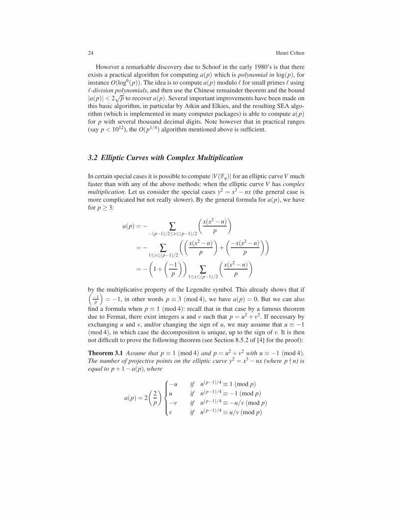
not difficult to prove the following theorem (see Section 8.5.2 of [4] for the proof):

Theorem 3.1 Assume that p ≡ 1 (mod 4) and p = u2 + v2 with u ≡ −1 (mod 4).The number of projective points on the elliptic curve y2 = x3− nx (where p ∤ n) is

equal to p+ 1− a(p), where

a(p) = 2

(2

p

)

−u if n(p−1)/4 ≡ 1 (mod p)

u if n(p−1)/4 ≡−1 (mod p)

−v if n(p−1)/4 ≡−u/v (mod p)

v if n(p−1)/4 ≡ u/v (mod p)


(note that one of these four cases must occur).

To apply this theorem from a computational standpoint we note the following

two facts:

(1) The quantity n(p−1)/4 mod p can be computed efficiently by the binary pow-

ering algorithm (in O(log3(p)) operations). It is however possible to compute it

more efficiently in O(log2(p)) operations using the quartic reciprocity law.

(2) The numbers u and v such that u2 + v2 = p can be computed efficiently (in

O(log2(p)) operations) using Cornacchia’s algorithm which is very easy to describe

but not so easy to prove. It is a variant of Euclid’s algorithm. It proceeds as follows:

• As a first step, we compute a square root of −1 modulo p, i.e., an x such that

x2 ≡−1 (mod p). This is done by choosing randomly a z ∈ [1, p−1] and computing

the Legendre symbol(

zp

)until it is equal to −1 (we can also simply try z = 2, 3,

...). Note that this is a fast computation. When this is the case, we have by definition

z(p−1)/2 ≡ −1 (mod p), hence x2 ≡ −1 (mod p) for x = z(p−1)/4 mod p. Reducing

x modulo p and possibly changing x into p−x, we normalize x so that p/2 < x < p.

•As a second step, we perform the Euclidean algorithm on the pair (p,x), writing

a0 = p, a1 = x, and an−1 = qnan+an+1 with 0≤ an+1 < an, and we stop at the exact

n for which a2n < p. It can be proved (this is the difficult part) that for this specific n

we have a2n +a2

n+1 = p, so up to exchange of u and v and/or change of signs, we can

take u = an and v = an+1.

Note that Cornacchia’s algorithm can easily be generalized to solving efficiently

u2 + dv2 = p or u2 + dv2 = 4p for any d ≥ 1, see Section 1.5.2 of[2] (incidentally

one can also solve this for d < 0, but it poses completely different problems since

there may be infinitely many solutions).

The above theorem is given for the special elliptic curves y2 = x3− nx which

have complex multiplication by the (ring of integers of the) field Q(i), but a similar

theorem is valid for all curves with complex multiplication, see Section 8.5.2 of [4].

3.3 Using Modular Forms of Weight 2

By Wiles’ celebrated theorem, the L-function of an elliptic curve is equal to the L-

function of a modular form of weight 2 for Γ0(N), where N is the conductor of the

curve. We do not need to give the precise definitions of these objects, but only a

specific example.

Let V be the elliptic curve with affine equation y2 + y = x3− x2. It has conductor

11. It can be shown using classical modular form methods (i.e., without Wiles’

theorem) that the global L-function L(V ;s) = ∑n≥1 a(n)/ns is the same as that of

the modular form of weight 2 over Γ0(11) given by

f (τ) = q ∏m≥1

(1− qm)2(1− q11m)2 ,

26 Henri Cohen

with q = exp(2π iτ). Even with no knowledge of modular forms, this simply means

that if we formally expand the product on the right hand side as

q ∏m≥1

(1− qm)2(1− q11m)2 = ∑n≥1

b(n)qn ,

we have b(n) = a(n) for all n, and in particular for n = p prime. We have already

seen this example above with a slightly different equation for the elliptic curve

(which makes no difference for its L-function outside of the primes 2 and 3).

We see that this gives an alternate method for computing a(p) by expanding the

infinite product. Indeed, the function

η(τ) = q1/24 ∏m≥1

(1− qm)

is a modular form of weight 1/2 with known expansion:

η(τ) = ∑n≥1

(12

n

)qn2/24 ,

and so using Fast Fourier Transform techniques for formal power series multipli-

cation we can compute all the coefficients a(n) simultaneously (as opposed to one

by one) for n≤ B in time O(B log2(B)). This amounts to computing each individual

a(n) in time O(log2(n)), so it seems to be competitive with the fast methods for el-

liptic curves with complex multiplication, but this is an illusion since we must store

all B coefficients, so it can be used only for B≤ 1012, say, far smaller than what can

be reached using Schoof’s algorithm, which is truly polynomial in log(p) for each

fixed prime p.

3.4 Higher Weight Modular Forms

It is interesting to note that the dichotomy between elliptic curves with or with-

out complex multiplication is also valid for modular forms of higher weight (again,

whatever that means, you do not need to know the definitions). For instance, con-

sider

∆(τ) = ∆24(τ) = η24(τ) = q ∏m≥1

(1− qm)24 := ∑n≥1

τ(n)qn .

The function τ(n) is a famous function called the Ramanujan τ function, and has

many important properties, analogous to those of the a(p) attached to an elliptic

curve (i.e., to a modular form of weight 2).

There are several methods to compute τ(p) for p prime, say. One is to do as

above, using FFT techniques. The running time is similar, but again we are lim-

ited to B ≤ 1012, say. A second more sophisticated method is to use the Eichler–

Selberg trace formula, which enables the computation of an individual τ(p) in time


O(p1/2+ε) for all ε > 0. A third very deep method, developed by Edixhoven, Cou-

veignes, et al., is a generalization of Schoof’s algorithm. While in principle polyno-

mial time in log(p), it is not yet practical compared to the preceding method.

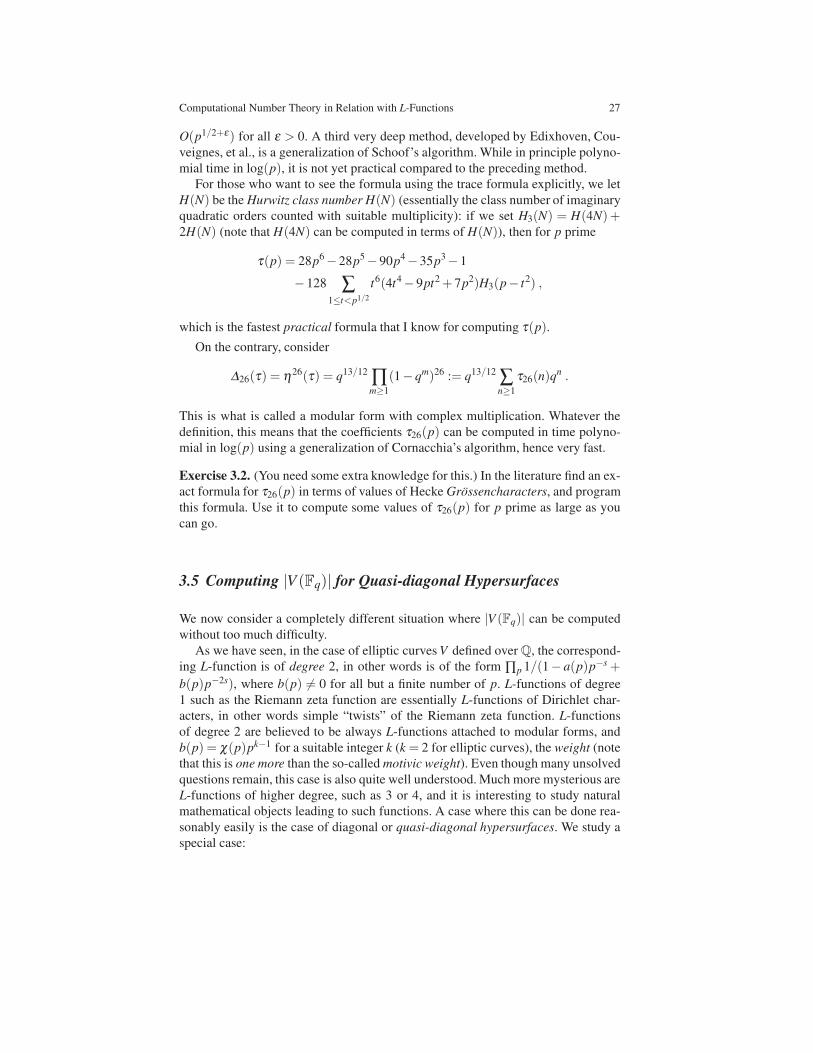
For those who want to see the formula using the trace formula explicitly, we let

H(N) be the Hurwitz class number H(N) (essentially the class number of imaginary

quadratic orders counted with suitable multiplicity): if we set H3(N) = H(4N)+2H(N) (note that H(4N) can be computed in terms of H(N)), then for p prime

τ(p) = 28p6− 28p5− 90p4− 35p3− 1

− 128 ∑1≤t<p1/2

t6(4t4− 9pt2 + 7p2)H3(p− t2) ,

which is the fastest practical formula that I know for computing τ(p).

On the contrary, consider

∆26(τ) = η26(τ) = q13/12 ∏m≥1

(1− qm)26 := q13/12 ∑n≥1

τ26(n)qn .

This is what is called a modular form with complex multiplication. Whatever the

definition, this means that the coefficients τ26(p) can be computed in time polyno-

mial in log(p) using a generalization of Cornacchia’s algorithm, hence very fast.

Exercise 3.2. (You need some extra knowledge for this.) In the literature find an ex-

act formula for τ26(p) in terms of values of Hecke Grossencharacters, and program

this formula. Use it to compute some values of τ26(p) for p prime as large as you

can go.

3.5 Computing |V (Fq)| for Quasi-diagonal Hypersurfaces

We now consider a completely different situation where |V (Fq)| can be computed

without too much difficulty.

As we have seen, in the case of elliptic curves V defined over Q, the correspond-

ing L-function is of degree 2, in other words is of the form ∏p 1/(1− a(p)p−s +

b(p)p−2s), where b(p) 6= 0 for all but a finite number of p. L-functions of degree

1 such as the Riemann zeta function are essentially L-functions of Dirichlet char-

acters, in other words simple “twists” of the Riemann zeta function. L-functions

of degree 2 are believed to be always L-functions attached to modular forms, and

b(p) = χ(p)pk−1 for a suitable integer k (k = 2 for elliptic curves), the weight (note

that this is one more than the so-called motivic weight). Even though many unsolved

questions remain, this case is also quite well understood. Much more mysterious are

L-functions of higher degree, such as 3 or 4, and it is interesting to study natural

mathematical objects leading to such functions. A case where this can be done rea-

sonably easily is the case of diagonal or quasi-diagonal hypersurfaces. We study a

special case:

28 Henri Cohen

Definition 3.3. Let m≥ 2, for 1≤ i≤ m let ai ∈ F∗q be nonzero, and let b ∈ Fq. The

quasi-diagonal hypersurface defined by this data is the hypersurface in Pm−1 defined

by the projective equation

∑1≤i≤m

aixmi − b ∏

1≤i≤m

xi = 0 .

When b = 0, it is a diagonal hypersurface.

Of course, we could study more general equations, for instance where the degree

is not equal to the number of variables, but we stick to this special case.

To compute the number of (projective) points on this hypersurface, we need an

additional definition:

Definition 3.4. We let ω be a generator of the group of characters of F∗q, either with

values in C, or in the p-adic field Cp (do not worry if you are not familiar with this).

Indeed, by a well-known theorem of elementary algebra, the multiplicative group

F∗q of a finite field is cyclic, so its group of characters, which is non-canonically

isomorphic to F∗q, is also cyclic, so ω indeed exists.

It is not difficult to prove the following theorem:

Theorem 3.5 Assume that gcd(m,q−1) = 1 and b 6= 0, and set B = ∏1≤i≤m(ai/b).If V is the above quasi-diagonal hypersurface, the number |V (Fq)| of affine points

on V is given by

|V (Fq)|= qm−1 +(−1)m−1 + ∑1≤n≤q−2

ω−n(B)Jm(ωn, . . . ,ωn) ,

where Jm is the m-variable Jacobi sum.

We will study in great detail below the definition and properties of Jm.

Note that the number of projective points is simply (|V (Fq)|− 1)/(q− 1).There also exists a more general theorem with no restriction on gcd(m,q− 1),

which we do not give.

The occurrence of Jacobi sums is very natural and frequent in point counting

results. It is therefore important to look at efficient ways to compute them, and this

is what we do in the next section, where we also give complete definitions and basic

results.

4 Gauss and Jacobi Sums

In this long section, we study in great detail Gauss and Jacobi sums. Most results

are standard, and I would like to emphasize that almost all of them can be proved

with little difficulty by easy algebraic manipulations.


4.1 Gauss Sums over Fq

We can define and study Gauss and Jacobi sums in two different contexts: first, and

most importantly, over finite fields Fq, with q = p f a prime power (note that from

now on we write q = p f and not q = pn). Second, over the ring Z/NZ. The two

notions coincide when N = q = p is prime, but the methods and applications are

quite different.

To give the definitions over Fq we need to recall some fundamental (and easy)

results concerning finite fields.

Proposition 4.1. Let p be a prime, f ≥ 1, and Fq be the finite field with q = p f

elements, which exists and is unique up to isomorphism.

1. The map φ such that φ(x) = xp is a field isomorphism from Fq to itself leaving

Fp fixed. It is called the Frobenius map.

2. The extension Fq/Fp is a normal (i.e., separable and Galois) field extension, with

Galois group which is cyclic of order f generated by φ .

In particular, we can define the trace TrFq/Fpand the norm N Fq/Fp

, and we have

the formulas (where from now on we omit Fq/Fp for simplicity):

Tr(x) = ∑0≤ j≤ f−1

xp j

and N (x) = ∏0≤ j≤ f−1

xp j

= x(p f−1)/(p−1) = x(q−1)/(p−1) .

Definition 4.2. Let χ be a character from F∗q to an algebraically closed field C of

characteristic 0. For a ∈ Fq we define the Gauss sum g(χ ,a) by

g(χ ,a) = ∑x∈F∗q

χ(x)ζTr(ax)p ,

where ζp is a fixed primitive pth root of unity in C. We also set g(χ) = g(χ ,1).

Note that strictly speaking this definition depends on the choice of ζp. However,

if ζ ′p is some other primitive pth root of unity we have ζ ′p = ζ kp for some k ∈ F∗p, so

∑x∈F∗q

χ(x)ζ ′pTr(ax)

= g(χ ,ka) .

In fact it is trivial to see (this follows from the next proposition) that g(χ ,ka) =χ−1(k)g(χ ,a).

Definition 4.3. We define ε to be the trivial character, i.e., such that ε(x) = 1 for all

x ∈ F∗q. We extend characters χ to the whole of Fq by setting χ(0) = 0 if χ 6= ε and

ε(0) = 1.

Note that this apparently innocuous definition of ε(0) is crucial because it sim-

plifies many formulas. Note also that the definition of g(χ ,a) is a sum over x ∈ F∗qand not x ∈ Fq, while for Jacobi sums we will use all of Fq.

30 Henri Cohen

Exercise 4.4. 1. Show that g(ε,a) =−1 if a ∈ F∗q and g(ε,0) = q− 1.

2. If χ 6= ε , show that g(χ ,0) = 0, in other words that

∑x∈Fq

χ(x) = 0

(here it does not matter if we sum over Fq or F∗q).

3. Deduce that if χ1 6= χ2 then

∑x∈F∗q

χ1(x)χ−12 (x) = 0 .

This relation is called for evident reasons orthogonality of characters.

4. Dually, show that if x 6= 0,1 we have ∑χ χ(x) = 0, where the sum is over all

characters of F∗q.

Because of this exercise, if necessary we may assume that χ 6= ε and/or that

a 6= 0.

Exercise 4.5. Let χ be a character of F∗q of exact order n.

1. Show that n | (q−1) and that χ(−1) = (−1)(q−1)/n. In particular, if n is odd and

p > 2 we have χ(−1) = 1.

2. Show that g(χ ,a) ∈ Z[ζn,ζp], where as usual ζm denotes a primitive mth root of

unity.

Proposition 4.6. 1. If a 6= 0 we have

g(χ ,a) = χ−1(a)g(χ) .

2. We have

g(χ−1) = χ(−1)g(χ) .

3. We have

g(χ p,a) = χ1−p(a)g(χ ,a) .

4. If χ 6= ε we have

|g(χ)|= q1/2 .

4.2 Jacobi Sums over Fq

Recall that we have extended characters of F∗q by setting χ(0) = 0 if χ 6= ε and

ε(0) = 1.

Definition 4.7. For 1≤ j ≤ k let χ j be characters of F∗q. We define the Jacobi sum

Jk(χ1, . . . ,χk;a) = ∑x1+···+xk=a

χ1(x1) · · ·χk(xk)


and Jk(χ1, . . . ,χk) = Jk(χ1, . . . ,χk;1).

Note that, as mentioned above, we do not exclude the cases where some xi = 0,

using the convention of Definition 4.3 for χ(0).The following easy lemma shows that it is only necessary to study Jk(χ1, . . . ,χk):

Lemma 4.8. Set χ = χ1 · · ·χk.

1. If a 6= 0 we have

Jk(χ1, . . . ,χk;a) = χ(a)Jk(χ1, . . . ,χk) .

2. If a = 0, abbreviating Jk(χ1, . . . ,χk;0) to Jk(0) we have

Jk(0) =

qk−1 if χ j = ε for all j ,

0 if χ 6= ε ,

χk(−1)(q− 1)Jk−1(χ1, . . . ,χk−1) if χ = ε and χk 6= ε .

As we have seen, a Gauss sum g(χ) belongs to the rather large ring Z[ζq−1,ζp](and in general not to a smaller ring). The advantage of Jacobi sums is that they

belong to the smaller ring Z[ζq−1], and as we are going to see, that they are closely

related to Gauss sums. Thus, when working algebraically, it is almost always bet-

ter to use Jacobi sums instead of Gauss sums. On the other hand, when working

analytically (for instance in C or Cp), it may be better to work with Gauss sums:

we will see below the use of root numbers (suggested by Louboutin), and of the

Gross–Koblitz formula.

Note that J1(χ1) = 1. Outside of this trivial case, the close link between Gauss

and Jacobi sums is given by the following easy proposition, whose apparently tech-

nical statement is only due to the trivial character ε: if none of the χ j nor their

product is trivial, we have the simple formula given by (3).

Proposition 4.9. Denote by t the number of χ j equal to the trivial character ε , and

as above set χ = χ1 . . .χk.

1. If t = k then Jk(χ1, . . . ,χk) = qk−1.

2. If 1≤ t ≤ k− 1 then Jk(χ1, . . . ,χk) = 0.

3. If t = 0 and χ 6= ε then

Jk(χ1, . . . ,χk) =g(χ1) · · ·g(χk)

g(χ1 · · ·χk)=

g(χ1) · · ·g(χk)

g(χ).

4. If t = 0 and χ = ε then

Jk(χ1, . . . ,χk) =−g(χ1) · · ·g(χk)

q

=−χk(−1)g(χ1) · · ·g(χk−1)

g(χ1 · · ·χk−1)=−χk(−1)Jk−1(χ1, . . . ,χk−1) .

32 Henri Cohen

In particular, in this case we have

g(χ1) · · ·g(χk) = χk(−1)qJk−1(χ1, . . . ,χk−1) .

Corollary 4.10. With the same notation, assume that k ≥ 2 and all the χ j are non-

trivial. Setting ψ = χ1 · · ·χk−1, we have the following recursive formula:

Jk(χ1, . . . ,χk) =

{Jk−1(χ1, . . . ,χk−1)J2(ψ ,χk) if ψ 6= ε ,

χk−1(−1)qJk−2(χ1, . . . ,χk−2) if ψ = ε .

The point of this recursion is that the definition of a k-fold Jacobi sum Jk involves

a sum over qk−1 values for x1, . . . ,xk−1, the last variable xk being determined by

xk = 1− x1− ·· · − xk−1, so neglecting the time to compute the χ j(x j) and their

product (which is a reasonable assumption), using the definition takes time O(qk−1).On the other hand, using the above recursion boils down at worst to computing k−1

Jacobi sums J2, for a total time of O((k−1)q). Nonetheless, we will see that in some

cases it is still better to use directly Gauss sums and formula (3) of the proposition.

Since Jacobi sums J2 are the simplest and the above recursion in fact shows that

one can reduce to J2, we will drop the subscript 2 and simply write J(χ1,χ2). Note

that

J(χ1,χ2) = ∑x∈Fq

χ1(x)χ2(1− x) ,

where the sum is over the whole of Fq and not Fq \{0,1} (which makes a difference

only if one of the χi is trivial). More precisely it is clear that J(ε,ε) = q2, and that

if χ 6= ε we have J(χ ,ε) = ∑x∈Fqχ(x) = 0, which are special cases of Proposition

4.9.

Exercise 4.11. Let n | (q− 1) be the order of χ . Prove that g(χ)n ∈ Z[ζn].

Exercise 4.12. Assume that none of the χ j is equal to ε , but that their product χ is

equal to ε . Prove that (using the same notation as in Lemma 4.8):

Jk(0) =

(1− 1

q

)g(χ1) · · ·g(χk) .

Exercise 4.13. Prove the following reciprocity formula for Jacobi sums: if the χ j

are all nontrivial and χ = χ1 · · ·χk, we have

Jk(χ−11 , . . . ,χ−1

k ) =qk−1−δ

Jk(χ1, . . . ,χk),

where δ = 1 if χ = ε , and otherwise δ = 0.


4.3 Applications of J(χ ,χ)

In this short subsection we give without proof a couple of applications of the spe-

cial Jacobi sums J(χ ,χ). Once again the proofs are not difficult. We begin by the

following result, which is a special case of the Hasse–Davenport relations that we

will give below.

Lemma 4.14. Assume that q is odd, and let ρ be the unique character of order 2 on

F∗q. For any nontrivial character χ we have

χ(4)J(χ ,χ) = J(χ ,ρ) .

Equivalently, if χ 6= ρ we have

g(χ)g(χρ) = χ−1(4)g(ρ)g(χ2) .

Exercise 4.15. 1. Prove this lemma.

2. Show that g(ρ)2 = (−1)(q−1)/2q.

Proposition 4.16. 1. Assume that q≡ 1 (mod 4), let χ be one of the two characters

of order 4 on F∗q, and write J(χ ,χ) = a+bi. Then q = a2 +b2, 2 | b, and a≡−1

(mod 4).2. Assume that q≡ 1 (mod 3), let χ be one of the two characters of order 3 on F∗q,

and write J(χ ,χ) = a+bρ , where ρ = ζ3 is a primitive cube root of unity. Then

q = a2− ab+ b2, 3 | b, a≡−1 (mod 3), and a+ b≡ q− 2 (mod 9).3. Let p≡ 2 (mod 3), q = p2m ≡ 1 (mod 3), and let χ be one of the two characters

of order 3 on F∗q. We have

J(χ ,χ) = (−1)m−1 pm = (−1)m−1q1/2 .

Corollary 4.17. 1. (Fermat.) Any prime p≡ 1 (mod 4) is a sum of two squares.

2. Any prime p ≡ 1 (mod 3) is of the form a2− ab+ b2 with 3 | b, or equivalently

4p = (2a− b)2+ 27(b/3)2 is of the form c2 + 27d2.

3. (Gauss.) p ≡ 1 (mod 3) is itself of the form p = u2 + 27v2 if and only if 2 is a

cube in F∗p.

Exercise 4.18. Assuming the proposition, prove the corollary.

4.4 The Hasse–Davenport Relations

All the results that we have given up to now on Gauss and Jacobi sums have rather

simple proofs, which is one of the reasons we have not given them. Perhaps sur-

prisingly, there exist other important relations which are considerably more difficult

to prove. Before giving them, it is instructive to explain how one can “guess” their

existence, if one knows the classical theory of the gamma function Γ (s) (of course

34 Henri Cohen

skip this part if you do not know it, since it would only confuse you, or read the

appendix).

Recall that Γ (s) is defined (at least for ℜ(s)> 0) by

Γ (s) =∫ ∞

0e−ttsdt/t ,

and the beta function B(a,b) by B(a,b) =∫ 1

0 ta−1(1− t)b−1 dt. The function e−t

transforms sums into products, so is an additive character, analogous to ζ tp. The

function ts transforms products into products, so is a multiplicative character, anal-

ogous to χ(t) (dt/t is simply the Haar invariant measure on R>0). Thus Γ (s) is a

continuous analogue of the Gauss sum g(χ).Similarly, since J(χ1,χ2) = ∑t χ1(t)χ2(1− t), we see the similarity with the

function B. Thus, it does not come too much as a surprise that analogous formu-

las are valid on both sides. To begin with, it is not difficult to show that B(a,b) =Γ (a)Γ (b)/Γ (a+ b), exactly analogous to J(χ1,χ2) = g(χ1)g(χ2)/g(χ1χ2). The

analogue of Γ (s)Γ (−s) =−π/(ssin(sπ)) is

g(χ)g(χ−1) = χ(−1)q .

But it is well-known that the gamma function has a duplication formula Γ (s)Γ (s+1/2)= 21−2sΓ (1/2)Γ (2s), and more generally a multiplication (or distribution) for-

mula. This duplication formula is clearly the analogue of the formula

g(χ)g(χρ) = χ−1(4)g(ρ)g(χ2)

given above. The Hasse–Davenport product relation is the analogue of the distribu-

tion formula for the gamma function.

Theorem 4.19 Let ρ be a character of exact order m dividing q− 1. For any char-

acter χ of F∗q we have

∏0≤a<m

g(χρa) = χ−m(m)k(p, f ,m)q(m−1)/2g(χm) ,

where k(p, f ,m) is the fourth root of unity given by

k(p, f ,m) =

( p

m

) f

if m is odd,

(−1) f+1

((−1)m/2+1m/2

p

) f(−1

p

) f/2

if m is even,

where (−1) f/2 is to be understood as i f when f is odd.

Remark 4.20. For some reason, in the literature this formula is usually stated in the

weaker form where the constant k(p, f ,m) is not given explicitly.


Contrary to the proof of the distribution formula for the gamma function, the

proof of this theorem is quite long. There are essentially two completely different

proofs: one using classical algebraic number theory, and one using p-adic analysis.

The latter is simpler and gives directly the value of k(p, f ,m). See Section 3.7.2 of

[4] and Section 11.7.4 of [5] for both detailed proofs.

Gauss sums satisfy another type of nontrivial relation, also due to Hasse–

Davenport, the so-called lifting relation, as follows:

Theorem 4.21 Let Fqn/Fq be an extension of finite fields, let χ be a character of

F∗q, and define the lift of χ to Fqn by the formula χ (n) = χ ◦N Fqn/Fq. We have

g(χ (n)) = (−1)n−1g(χ)n .

This relation is essential in the initial proof of the Weil conjectures for diagonal

hypersurfaces done by Weil himself. This is not surprising, since we have seen in

Theorem 3.5 that |V (Fq)| is closely related to Jacobi sums, hence also to Gauss

sums.

5 Practical Computations of Gauss and Jacobi Sums

As above, let ω be a character of order exactly q− 1, so that ω is a generator of

the group of characters of F∗q. For notational simplicity, we will write J(r1, . . . ,rk)instead of J(ωr1 , . . . ,ωrk). Let us consider the specific example of efficient compu-

tation of the quantity

S(q;z) = ∑0≤n≤q−2

ω−n(z)J5(n,n,n,n,n) ,

which occurs in the computation of the Hasse–Weil zeta function of a quasi-diagonal

threefold, see Theorem 3.5.

5.1 Elementary Methods

By the recursion of Corollary 4.10, we have generically (i.e., except for special

values of n which will be considered separately):

J5(n,n,n,n,n) = J(n,n)J(2n,n)J(3n,n)J(4n,n) .

Since J(n,an) = ∑x ωn(x)ωan(1− x), the cost of computing J5 as written is O(q),

where here and after we write O(qα) to mean O(qα+ε) for all ε > 0 (soft-O nota-

tion). Thus computing S(q;z) by this direct method requires time O(q2).

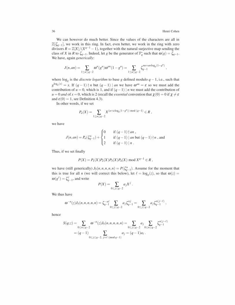
36 Henri Cohen

We can however do much better. Since the values of the characters are all in

Z[ζq−1], we work in this ring. In fact, even better, we work in the ring with zero

divisors R = Z[X ]/(Xq−1− 1), together with the natural surjective map sending the

class of X in R to ζq−1. Indeed, let g be the generator of F∗q such that ω(g) = ζq−1.

We have, again generically:

J(n,an) = ∑1≤u≤q−2

ωn(gu)ωan(1− gu) = ∑1≤u≤q−2

ζnu+an logg(1−gu)

q−1 ,

where logg is the discrete logarithm to base g defined modulo q− 1, i.e., such that

glogg(x) = x. If (q− 1) ∤ n but (q− 1) | an we have ωan = ε so we must add the

contribution of u = 0, which is 1, and if (q− 1) | n we must add the contribution of

u = 0 and of x = 0, which is 2 (recall the essential convention that χ(0) = 0 if χ 6= εand ε(0) = 1, see Definition 4.3).

In other words, if we set

Pa(X) = ∑1≤u≤q−2

X (u+a logg(1−gu)) mod (q−1) ∈ R ,

we have

J(n,an) = Pa(ζnq−1)+

0 if (q− 1) ∤ an ,

1 if (q− 1) | an but (q− 1) ∤ n , and

2 if (q− 1) | n .

Thus, if we set finally

P(X) = P1(X)P2(X)P3(X)P4(X) mod Xq−1 ∈ R ,

we have (still generically) J5(n,n,n,n,n) = P(ζ nq−1). Assume for the moment that

this is true for all n (we will correct this below), let ℓ = logg(z), so that ω(z) =

ω(gℓ) = ζ ℓq−1, and write

P(X) = ∑0≤ j≤q−2

a jXj .

We thus have

ω−n(z)J5(n,n,n,n,n) = ζ−nℓq−1 ∑

0≤ j≤q−2

a jζn jq−1 = ∑

0≤ j≤q−2

a jζn( j−ℓ)q−1 ,

hence

S(q;z) = ∑0≤n≤q−2

ω−n(z)J5(n,n,n,n,n) = ∑0≤ j≤q−2

a j ∑0≤n≤q−2

ζn( j−ℓ)q−1

= (q− 1) ∑0≤ j≤q−2, j≡ℓ (mod q−1)

a j = (q− 1)aℓ .


The result is thus immediate as soon as we know the coefficients of the polynomial

P. Since there exist fast methods for computing discrete logarithms, this leads to a

O(q) method for computing S(q;z).

To obtain the correct formula, we need to adjust for the special n for which

J5(n,n,n,n,n) is not equal to J(n,n)J(n,2n)J(n,3n)J(n,4n), which are the same

for which (q− 1) | an for some a such that 2 ≤ a ≤ 4, together with a = 5. This is

easy but boring, and should be skipped on first reading.

1. For n = 0 we have J5(n,n,n,n,n) = q4, and on the other hand P(1) = (J(0,0)−2)4 = (q− 2)4, so the correction term is q4− (q− 2)4 = 8(q− 1)(q2− 2q+ 2).

2. For n = (q− 1)/2 (if q is odd) we have

J5(n,n,n,n,n) = g(ωn)5/g(ω5n) = g(ωn)4 = g(ρ)4

since 5n ≡ n (mod q− 1), where ρ is the character of order 2, and we have

g(ρ)2 = (−1)(q−1)/2q, so J5(n,n,n,n,n) = q2. On the other hand

P(ζ nq−1) = J(ρ ,ρ)(J(ρ ,2ρ)− 1)J(ρ ,ρ)(J(ρ ,2ρ)− 1)

= J(ρ ,ρ)2 = g(ρ)4/q2 = 1 ,

so the correction term is ρ(z)(q2− 1).3. For n = ±(q− 1)/3 (if q ≡ 1 (mod 3)), writing χ3 = ω(q−1)/3, which is one of

the two cubic characters, we have

J5(n,n,n,n,n) = g(ωn)5/g(ω5n) = g(ωn)5/g(ω−n)

= g(ωn)6/(g(ω−n)g(ωn)) = g(ωn)6/q

= qJ(n,n)2

(check all this). On the other hand

P(ζ nq−1) = J(n,n)J(n,2n)(J(n,3n)− 1)J(n,4n)

=g(ωn)2

g(ω2n)

g(ωn)g(ω2n)

q

g(ωn)2

g(ω2n)

=g(ωn)5

qg(ω−n)=

g(ωn)6

q2= J(n,n)2 ,

so the correction term is 2(q− 1)ℜ(χ−13 (z)J(χ3,χ3)

2).

4. For n = ±(q− 1)/4 (if q ≡ 1 (mod 4)), writing χ4 = ω(q−1)/4, which is one of

the two quartic characters, we have

J5(n,n,n,n,n) = g(ωn)5/g(ω5n) = g(ωn)4 = ωn(−1)qJ3(n,n,n) .

In addition, we have

J3(n,n,n) = J(n,n)J(n,2n) = ωn(4)J(n,n)2 = ρ(2)J(n,n)2 ,

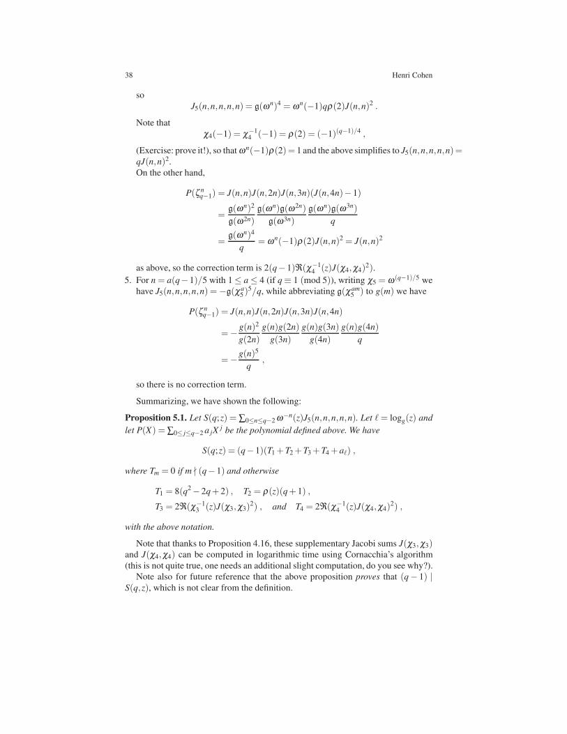
38 Henri Cohen

so

J5(n,n,n,n,n) = g(ωn)4 = ωn(−1)qρ(2)J(n,n)2 .

Note that

χ4(−1) = χ−14 (−1) = ρ(2) = (−1)(q−1)/4 ,

(Exercise: prove it!), so that ωn(−1)ρ(2)= 1 and the above simplifies to J5(n,n,n,n,n)=qJ(n,n)2.

On the other hand,

P(ζ nq−1) = J(n,n)J(n,2n)J(n,3n)(J(n,4n)− 1)

=g(ωn)2

g(ω2n)

g(ωn)g(ω2n)

g(ω3n)

g(ωn)g(ω3n)

q

=g(ωn)4

q= ωn(−1)ρ(2)J(n,n)2 = J(n,n)2

as above, so the correction term is 2(q− 1)ℜ(χ−14 (z)J(χ4,χ4)

2).

5. For n = a(q−1)/5 with 1≤ a≤ 4 (if q≡ 1 (mod 5)), writing χ5 = ω(q−1)/5 we

have J5(n,n,n,n,n) =−g(χa5 )

5/q, while abbreviating g(χam5 ) to g(m) we have

P(ζ nq−1) = J(n,n)J(n,2n)J(n,3n)J(n,4n)

=− g(n)2

g(2n)

g(n)g(2n)

g(3n)

g(n)g(3n)

g(4n)

g(n)g(4n)

q

=−g(n)5

q,

so there is no correction term.

Summarizing, we have shown the following:

Proposition 5.1. Let S(q;z) = ∑0≤n≤q−2 ω−n(z)J5(n,n,n,n,n). Let ℓ= logg(z) and

let P(X) = ∑0≤ j≤q−2 a jXj be the polynomial defined above. We have

S(q;z) = (q− 1)(T1 +T2 +T3 +T4 + aℓ) ,

where Tm = 0 if m ∤ (q− 1) and otherwise

T1 = 8(q2− 2q+ 2) , T2 = ρ(z)(q+ 1) ,

T3 = 2ℜ(χ−13 (z)J(χ3,χ3)

2) , and T4 = 2ℜ(χ−14 (z)J(χ4,χ4)

2) ,

with the above notation.

Note that thanks to Proposition 4.16, these supplementary Jacobi sums J(χ3,χ3)and J(χ4,χ4) can be computed in logarithmic time using Cornacchia’s algorithm

(this is not quite true, one needs an additional slight computation, do you see why?).

Note also for future reference that the above proposition proves that (q− 1) |S(q,z), which is not clear from the definition.


5.2 Sample Implementations

For simplicity, assume that q = p is prime. I have written simple implementations

of the computation of S(q;z). In the first implementation, I use the naıve formula

expressing J5 in terms of J(n,an) and sum on n, except that I use the reciprocity

formula which gives J5(−n,−n,−n,−n,−n) in terms of J5(n,n,n,n,n) to sum only

over (p− 1)/2 terms instead of p− 1. Of course to avoid recomputation, I precom-

pute a discrete logarithm table.

The timings for p ≈ 10k for k = 2, 3, and 4 are 0.03, 1.56, and 149 seconds

respectively, compatible with O(q2) time.

On the other hand, implementing in a straightforward manner the algorithm given

by the above proposition gives timings for p ≈ 10k for k = 2, 3, 4, 5, 6, and 7 of

0, 0.02, 0.08, 0.85, 9.90, and 123 seconds respectively, of course much faster and

compatible with O(q) time.

The main drawback of this method is that it requires O(q) storage: it is thus

applicable only for q≤ 108, say, which is more than sufficient for many applications,

but of course not for all. For instance, the case p ≈ 107 mentioned above already

required a few gigabytes of storage.

5.3 Using Theta Functions

A completely different way of computing Gauss and Jacobi sums has been sug-

gested by S. Louboutin. It is related to the theory of L-functions of Dirichlet char-

acters that we study below, and in our context is valid only for q = p prime, not for

prime powers, but in the context of Dirichlet characters it is valid in general (simply

replace p by N and Fp by Z/NZ in the following formulas when χ is a primitive

character of conductor N, see below for definitions):

Definition 5.2. Let χ be a character on Fp, and let e = 0 or 1 be such that χ(−1) =(−1)e. The theta function associated to χ is the function defined on the upper half-

plane by

Θ(χ ,τ) = 2 ∑m≥1

meχ(m)eiπm2τ/p .

The main property of this function, which is a direct consequence of the Pois-

son summation formula, and is equivalent to the functional equation of Dirichlet

L-functions, is as follows:

Proposition 5.3. We have the functional equation

Θ(χ ,−1/τ) = ω(χ)(τ/i)(2e+1)/2Θ(χ−1,τ) ,

with the principal determination of the square root, and where ω(χ)= g(χ)/(iep1/2)is the so-called root number.

40 Henri Cohen

Corollary 5.4. If χ(−1) = 1 we have

g(χ) = p1/2 ∑m≥1 χ(m)exp(−πm2/pt)

t1/2 ∑m≥1 χ−1(m)exp(−πm2t/p)

and if χ(−1) =−1 we have

g(χ) = p1/2i∑m≥1 χ(m)mexp(−πm2/pt)

t3/2 ∑m≥1 χ−1(m)mexp(−πn2t/p)

for any t such that the denominator does not vanish.

Note that the optimal choice of t is t = 1, and (at least for p prime) it seems that

the denominator never vanishes (there are counterexamples when p is not prime, but

apparently only four, see [9]).

It follows from this corollary that g(χ) can be computed numerically as a

complex number in O(p1/2) operations. Thus, if χ1 and χ2 are nontrivial charac-

ters such that χ1χ2 6= ε (otherwise J(χ1,χ2) is trivial to compute), the formula

J(χ1,χ2) = g(χ1)g(χ2)/g(χ1χ2) allows the computation of J2 numerically as a

complex number in O(p1/2) operations.

To recover J itself as an algebraic number we could either compute all its conju-

gates, but this would require more time than the direct computation of J, or possibly

use the LLL algorithm, which although fast, would also require some time. In prac-

tice, to perform computations such as that of the sum S(q;z) above, we only need

J to sufficient accuracy: we perform all the elementary operations in C, and since

we know that at the end the result will be an integer for which we know an upper

bound, we thus obtain a proven exact result.

More generally, we have generically J5(n,n,n,n,n)= g(ωn)5/g(ω5n), which can

thus be computed in O(p1/2) operations. It follows that S(p;z) can be computed in

O(p3/2) operations, which is slower than the elementary method seen above. The

main advantage is that we do not need much storage: more precisely, we want to

compute S(p;z) to sufficiently small accuracy that we can recognize it as an integer,

so a priori up to an absolute error of 0.5. However, we have seen that (p− 1) |S(p;z): it is thus sufficient to have an absolute error less than (p− 1)/2 thus at

worse each of the p− 1 terms in the sum to an absolute error less than 1/2. Since

generically |J5(n,n,n,n,n)|= p2, we need a relative error less than 1/(2p2), so less

than 1/(10p2) on each Gauss sum. In practice of course this is overly pessimistic,

but it does not matter. For p≤ 109, this means that 19 decimal digits suffice.

The main term in the theta function computation (with t = 1) is exp(−πm2/p), so

we need exp(−πm2/p)≤ 1/(100p2), say, in other words πm2/p ≥ 4.7+ 2log(p),so m2 ≥ p(1.5+ 0.7log(p)).

This means that we will need the values of ω(m) only up to this limit, of the

order of O((p log(p))1/2), considerably smaller than p. Thus, instead of computing

a full discrete logarithm table, which takes some time but more importantly a lot

of memory, we compute only discrete logarithms up to that limit, using specific


algorithms for doing so which exist in the literature, some of which being quite

easy.

A straightforward implementation of this method gives timings for k = 2, 3, 4,

and 5 of 0.02, 0.40, 16.2, and 663 seconds respectively, compatible with O(p3/2)time. This is faster than the completely naıve method, but slower than the method

explained above. Its advantage is that it requires much less memory. For p around

107, however, it is much too slow so this method is rather useless. We will see that

its usefulness is mainly in the context where it was invented, i.e., for L-functions of

Dirichlet characters.

5.4 Using the Gross–Koblitz Formula

This section is of a higher mathematical level than the preceding ones, but is very

important since it gives the best method for computing Gauss (and Jacobi) sums.

We refer to Sections 11.6 and 11.7 of [5] for complete details, and urge the reader

to try to understand what follows.

In the preceding sections, we have considered Gauss sums as belonging to a

number of different rings: the ring Z[ζq−1,ζp] or the field C of complex numbers,

and for Jacobi sums the ring Z[ζq−1], but also the ring Z[X ]/(Xq−1− 1), and again

the field C.

In number theory there exist other algebraically closed fields which are useful in

many contexts, the fields Cℓ of ℓ-adic numbers, one for each prime number ℓ. These

fields come with a topology and analysis which are rather special: one of the main

things to remember is that a sequence of elements tends to 0 if and only the ℓ-adic

valuation of the elements (the largest exponent of ℓ dividing them) tends to infinity.

For instance 2m tends to 0 in C2, but in no other Cℓ, and 15m tends to 0 in C3 and in

C5.

The most important subrings of Cℓ are the ring Zℓ of ℓ-adic integers, the elements

of which can be written as x = a0 + a1ℓ+ · · ·+ akℓk + · · · with a j ∈ [0, ℓ− 1], and

its field of fractions Qℓ, which contains Q, whose elements can be represented in a

similar way as x = a−mℓ−m + a−(m−1)ℓ

−(m−1)+ · · ·+ a−1ℓ−1 + a0 + a1ℓ+ · · · .

In dealing with Gauss and Jacobi sums over Fq with q = p f , the only Cℓ which

is of use for us is the one with ℓ = p (in highbrow language, we are going to use

implicitly crystalline p-adic methods, while for ℓ 6= p it would be etale ℓ-adic meth-

ods).

Apart from this relatively strange topology, many definitions and results valid

on C have analogues in Cp. The main object that we will need in our context is

the analogue of the gamma function, naturally called the p-adic gamma function, in

the present case due to Morita (there is another one, see Section 11.5 of [5]), and

denoted Γp. Its definition is in fact quite simple:

Definition 5.5. For s ∈ Zp we define

42 Henri Cohen

Γp(s) = limm→s

(−1)m ∏0≤k<m

p∤k

k ,

where the limit is taken over any sequence of positive integers m tending to s for the

p-adic topology.

It is of course necessary to show that this definition makes sense, but this is not

difficult, and most of the important properties of Γp(s), analogous to those of Γ (s),can be deduced from it.

Exercise 5.6. Choose p = 5 and s = −1/4, so that p-adically s = 1/(1− 5) = 1+5+ 52+ 53 + · · · .1. Compute the right hand side of the above definition with small 5-adic accuracy

for m = 1, 1+ 5, and 1+ 5+ 52.

2. It is in fact easy to compute that

Γ5(−1/4) = 4+ 4 ·5+ 53+ 3 ·54+ 2 ·55+ 2 ·56+ 2 ·57+ 4 ·58+ · · ·

Using this, show that Γ5(−1/4)2/16 seems to be a 5-adic root of the polynomial

5X2 + 4X + 1. This is in fact true, see the Gross–Koblitz formula below.

We need a much deeper property of Γp(s) known as the Gross–Koblitz formula: it

is in fact an analogue of a formula for Γ (s) known as the Chowla–Selberg formula,

and it is also closely related to the Davenport–Hasse relations that we have seen

above.

The proof of the Gross–Koblitz formula was initially given using tools of crys-

talline cohomology, but an elementary proof due to A. Robert now exists, see for

instance Section 11.7 of [5] once again.

The Gross–Koblitz formula tells us that certain products of p-adic gamma func-

tions at rational arguments are in fact algebraic numbers, more precisely Gauss

sums (explaining their importance for us). This is quite surprising since usually

transcendental functions such as Γp take transcendental values.

To give a specific example, we have Γ5(1/4)2 = −2+√−1, where

√−1 is the

square root in Z5 congruent to 3 modulo 5. In view of the elementary properties

of the p-adic gamma function, this is equivalent to the result stated in the above

exercise as Γ5(−1/4)2 =−(16/5)(2+√−1).

Before stating the formula we need to collect a number of facts, both on classical

algebraic number theory and on p-adic analysis. None are difficult to prove, see

Chapter 4 of [4]. Recall that q = p f .

•We let K = Q(ζp) and L = K(ζq−1) = Q(ζq−1,ζp) = Q(ζp(q−1)), so that L/K

is an extension of degree φ(q− 1). There exists a unique prime ideal p of K above

p, and we have p= (1−ζp)ZK and pp−1 = pZK , and ZK/p≃ Fp. The prime ideal p

splits into a product of g = φ(q−1)/ f prime ideals P j of degree f in the extension

L/K, i.e., pZL =P1 · · ·Pg, and for any prime ideal P=P j we have ZL/P≃ Fq.

Exercise 5.7. Prove directly that for any f we have f | φ(p f − 1).


• Fix one of the prime ideals P as above. There exists a unique group isomor-

phism ω = ωP from (ZL/P)∗ to the group of (q−1)st roots of unity in L, such that

for all x ∈ (ZL/P)∗ we have ω(x)≡ x (mod P). It is called the Teichmuller charac-

ter, and it can be considered as a character of order q−1 on F∗q ≃ (ZL/P)∗. We can

thus instantiate the definition of a Gauss sum over Fq by defining it as g(ω−rP

) ∈ L.

• Let ζp be a primitive pth root of unity in Cp, fixed once and for all. There

exists a unique π ∈ Z[ζp] satisfying π p−1 = −p, π ≡ 1− ζp (mod π2), and we set

Kp =Qp(π)=Qp(ζp), and LP the completion of L at P. The field extension LP/Kp

is Galois, with Galois group isomorphic to Z/ fZ (which is the same as the Galois

group of Fq/Fp, where Fp (resp., Fq) is the so-called residue field of K (resp., L)).

•We set the following:

Definition 5.8. We define the p-adic Gauss sum by

gq(r) = ∑x∈LP , xq−1=1

x−rζTrLP/Kp

(x)

p ∈ LP .

Note that this depends on the choice of ζp, or equivalently of π . Since gq(r) and

g(ω−rP

) are algebraic numbers, it is clear that they are equal, although viewed in

fields having different topologies. Thus, results about gq(r) translate immediately

into results about g(ω−rP

), hence about general Gauss sums over finite fields.

The Gross–Koblitz formula is as follows:

Theorem 5.9 (Gross–Koblitz) Denote by s(r) the sum of digits in base p of the

integer r mod (q− 1), i.e., of the unique integer r′ such that r′ ≡ r (mod q− 1) and

0≤ r′ < q− 1. We have

gq(r) =−π s(r) ∏0≤i< f

Γp

({p f−ir

q− 1

}),

where {x} denotes the fractional part of x.

Let us show how this can be used to compute Gauss or Jacobi sums, and in

particular our sum S(q;z). Assume for simplicity that f = 1, in other words that

q = p: the right hand side is thus equal to −π s(r)Γp({pr/(p− 1)}). Since we can

always choose r such that 0 ≤ r < p− 1, we have s(r) = r and {pr/(p− 1)} ={r+r/(p−1)}= r/(p−1), so the RHS is−π rΓp(r/(p−1)). Now an easy property

of Γp is that it is differentiable: recall that p is “small” in the p-adic topology, so

r/(p− 1) is close to −r, more precisely r/(p− 1) = −r+ pr/(p− 1) (this is how

we obtained it in the first place!). Thus in particular, if p > 2 we have the Taylor

expansion

Γp(r/(p− 1)) = Γp(−r)+ (pr/(p− 1))Γ ′p(−r)+O(p2)

= Γp(−r)− prΓ ′p(−r)+O(p2) .

44 Henri Cohen

Since gq(r) depends only on r modulo p−1, we will assume that 0≤ r < p−1.

In that case it is easy to show from the definition that

Γp(−r) = 1/r! and Γ ′p(−r) = (−γp +Hr)/r! ,

where Hr = ∑1≤n≤r 1/n is the harmonic sum, and γp = −Γ ′p(0) is the p-adic ana-

logue of Euler’s constant.

Exercise 5.10. Prove these formulas, as well as the congruence for γp given below.

There exist infinite (p-adic) series enabling accurate computation of γp, but since

we only need it modulo p, we use the easily proved congruence γp ≡ ((p− 1)!+1)/p =Wp (mod p), the so-called Wilson quotient.

We will see below that, as a consequence of the Weil conjectures proved by

Deligne, it is sufficient to compute S(p;z) modulo p2. Thus, in the following p-adic

computation we only work modulo p2.

The Gross–Koblitz formula tells us that for 0≤ r < p− 1 we have

gq(r) =−π r

r!(1− pr(Hr−Wp)+O(p2)) .

It follows that for (p− 1) ∤ 5r we have

J(−r,−r,−r,−r,−r) =g(ωP)5

g(ω5P)

=gq(r)

5

gq(5r)= π f (r)(a+ bp+O(p2)) ,

where a and b will be computed below and

f (r) = 5r− (5r mod p− 1) = 5r− (5r− (p− 1)⌊5r/(p− 1)⌋)= (p− 1)⌊5r/(p− 1)⌋ ,

so that π f (r) = (−p)⌊5r/(p−1)⌋ since π p−1 = −p. Since we want the result modulo

p2, we consider three intervals together with special cases:

1. If r > 2(p− 1)/5 but (p− 1) ∤ 5r, we have

J(−r,−r,−r,−r,−r)≡ 0 (mod p2) .

2. If (p− 1)/5< r < 2(p− 1)/5 we have

J(−r,−r,−r,−r,−r)≡ (−p)(5r− (p− 1))!

r!5(mod p2) .

3. If 0 < r < (p− 1)/5 we have f (r) = 0 and 0≤ 5r < (p− 1) hence


J(−r,−r,−r,−r,−r) =(5r)!

r!5(1− 5pr(Hr−Wp)+O(p2))·

· (1+ 5pr(H5r−Wp)+O(p2))

≡ (5r)!

r!5(1+ 5pr(H5r−Hr)) (mod p2) .

4. Finally, if r = j(p− 1)/5 we have J(−r,−r,−r,−r,−r) = p4 ≡ 0 (mod p2) if

j = 0, and otherwise J(−r,−r,−r,−r,−r) = −gq(r)5/p, and since the p-adic

valuation of gq(r) is equal to r/(p− 1) = j/5, that of J(−r,−r,−r,−r,−r) is

equal to j− 1, which is greater or equal to 2 as soon as j ≥ 3. For j = 2, i.e.,

r = 2(p− 1)/5, we thus have

J(−r,−r,−r,−r,−r)≡ p1

r!5≡ (−p)

(5r− (p− 1))!

r!5(mod p2) ,

which is the same formula as for (p− 1)/5 < r ≤ 2(p− 1)/5. For j = 1, i.e.,

r = (p− 1)/5, we thus have

J(−r,−r,−r,−r,−r)≡− 1

r!5(1− 5pr(Hr−Wp)) (mod p2) ,

while on the other hand

(5r)! = (p− 1)! =−1+ pWp≡−1− p(p− 1)Wp≡−1− 5prWp ,

and H5r = Hp−1 ≡ 0 (mod p) (Wolstenholme’s congruence, easy), so

(5r)!

r!5(1+ 5pr(H5r−Hr))≡−

1

r!5(1− 5prHr)(1+ 5prWp)

≡− 1

r!5(1− 5pr(Hr−Wp)) (mod p2) ,

which is the same formula as for 0 < r < (p− 1)/5.

An important point to note is that we are working p-adically, but the final result

S(p;z) being an integer, it does not matter at the end. There is one small additional

detail to take care of: we have

S(p;z) = ∑0≤r≤p−2

ω−r(z)J(r,r,r,r,r)

= ∑0≤r≤p−2

ωr(z)J(−r,−r,−r,−r,−r) ,

so we must express ωr(z) in the p-adic setting. Since ω = ωP is the Teichmuller

character, in the p-adic setting it is easy to show that ω(z) is the p-adic limit of zpk

as k→ ∞. in particular ω(z)≡ z (mod p), but more precisely ω(z)≡ zp (mod p2).

46 Henri Cohen

Exercise 5.11. Let p ≥ 3. Assume that z ∈ Zp \ pZp (for instance that z ∈ Z\ pZ).

Prove that zpkhas a p-adic limit ω(z) when k→ ∞, that ω p−1(z) = 1, that ω(z)≡ z

(mod p), and ω(z)≡ zp (mod p2).

We have thus proved the following

Proposition 5.12. We have

S(p;z)≡ ∑0<r≤(p−1)/5

(5r)!

r!5(1+ 5pr(H5r−Hr))z

pr

− p ∑(p−1)/5<r≤2(p−1)/5

(5r− (p− 1))!

r!5zr (mod p2) .

In particular

S(p;z)≡ ∑0<r≤(p−1)/5

(5r)!

r!5zr (mod p) .

Remarks 5.13 1. Note that, as must be the case, all mention of p-adic numbers has

disappeared from this formula. We used the p-adic setting only in the proof. It

can be proved “directly”, but with some difficulty.

2. We used the Taylor expansion only to order 2. It is of course possible to use it to

any order, thus giving a generalization of the above proposition to any power of

p.

The point of giving all these details is as follows: it is easy to show that (p−1) | S(p;z) (in fact we have seen this in the elementary method above). We can

thus easily compute S(p;z) modulo p2(p− 1). On the other hand, it is possible

to prove (but not easy, it is part of the Weil conjectures proved by Deligne), that

|S(p;z)− p4|< 4p5/2. It follows that as soon as 8p5/2 < p2(p− 1), in other words

p≥ 67, the computation that we perform modulo p2 is sufficient to determine S(p;z)

exactly. It is clear that the time to perform this computation is O(p), and in fact much

faster than any that we have seen.

In fact, implementing in a reasonable way the algorithm given by the above

proposition gives timings for p ≈ 10k for k = 2, 3, 4, 5, 6, 7, and 8 of 0, 0.01,

0.03, 0.21, 2.13, 21.92, and 229.6 seconds respectively, of course much faster and

compatible with O(p) time. The great additional advantage is that we use very small

memory. This is therefore the best known method.

Numerical example: Choose p = 106 + 3 and z = 2. In 2.13 seconds we find

that S(p;z) ≡ a (mod p2) with a = 356022712041. Using the Chinese remainder

formula

S(p;z) = p4 +((a− (1+ a)p2) mod ((p− 1)p2)) ,

we immediately deduce that

S(p;z) = 1000012000056356142712140 .


Here is a summary of the timings (in seconds) that we have mentioned:

k 2 3 4 5 6 7 8

Naıve 0.03 1.56 149 ∗ ∗ ∗ ∗Theta 0.02 0.40 16.2 663 ∗ ∗ ∗

Mod Xq−1− 1 0 0.02 0.08 0.85 9.90 123 ∗Gross–Koblitz 0 0.01 0.03 0.21 2.13 21.92 229.6

Time for computing S(p;z) for p≈ 10k

6 Gauss and Jacobi Sums over Z/NZ

Another context in which one encounters Gauss sums is over finite rings such as

Z/NZ. The theory coincides with that over Fq when q = p = N is prime, but is

rather different otherwise. These other Gauss sums enter in the important theory of

Dirichlet characters.

6.1 Definitions

We recall the following definition:

Definition 6.1. Let χ be a (multiplicative) character from the multiplicative group

(Z/NZ)∗ of invertible elements of Z/NZ to the complex numbers C. We denote by

abuse of notation again by χ the map from Z to C defined by χ(x) = χ(x mod N)when x is coprime to N, and χ(x) = 0 if x is not coprime to N, and call it the Dirichlet

character modulo N associated to χ .

It is clear that a Dirichlet character satisfies χ(xy) = χ(x)χ(y) for all x and y,

that χ(x+N) = χ(x), and that χ(x) = 0 if and only if x is not coprime with N.

Conversely, it immediate that these properties characterize Dirichlet characters.

A crucial notion (which has no equivalent in the context of characters of F∗q) is

that of primitivity:

Assume that M | N. If χ is a Dirichlet character modulo M, we can transform

it into a character χN modulo N by setting χN(x) = χ(x) if x is coprime to N, and

χN(x) = 0 otherwise. We say that the characters χ and χN are equivalent. Con-

versely, if ψ is a character modulo N, it is not always true that one can find χmodulo M such that ψ = χN . If it is possible, we say that ψ can be defined modulo

M.

Definition 6.2. Let χ be a character modulo N. We say that χ is a primitive char-

acter if χ cannot be defined modulo M for any proper divisor M of N, i.e., for any

M | N such that M 6= N.

48 Henri Cohen

Exercise 6.3. Assume that N≡ 2 (mod 4). Show that there do not exist any primitive

characters modulo N.

Exercise 6.4. Assume that pa | N with p prime. Show that if χ is a primitive char-

acter modulo N, the order of χ (the smallest k such that χk is a trivial character) is

divisible by pa−1.

As we will see, questions about general Dirichlet characters can always be re-

duced to questions about primitive characters, and the latter have much nicer prop-

erties.

Proposition 6.5. Let χ be a character modulo N. There exists a divisor f of N called

the conductor of χ (this f has nothing to do with the f used above such that q= p f ),

having the following properties:

1. The character χ can be defined modulo f , in other words there exists a character

ψ modulo f such that χ = ψN using the notation above.

2. f is the smallest divisor of N having this property.

3. The character ψ is a primitive character modulo f .

There is also the notion of trivial character modulo N: however we must be

careful here, and we set the following:

Definition 6.6. The trivial character modulo N is the Dirichlet character associated

with the trivial character of (Z/NZ)∗. It is usually denoted by χ0 (but be careful,

the index N is implicit, so χ0 may represent different characters), and its values are

as follows: χ0(x) = 1 if x is coprime to N, and χ0(x) = 0 if x is not coprime to N.

In particular, χ0(0) = 0 if N 6= 1. The character χ0 can also be characterized as

the only character modulo N of conductor 1.

Definition 6.7. Let χ be a character modulo N. The Gauss sum associated to χ and

a ∈ Z is

g(χ ,a) = ∑x mod N

χ(x)ζ axN ,

and we write simply g(χ) instead of g(χ ,1).

The most important results concerning these Gauss sums is the following:

Proposition 6.8. Let χ be a character modulo N.

1. If a is coprime to N we have

g(χ ,a) = χ−1(a)g(χ) = χ(a)g(χ) ,

and more generally g(χ ,ab) = χ−1(a)g(χ ,b) = χ(a)g(χ ,b).2. If χ is a primitive character, we have

g(χ ,a) = χ(a)g(χ)

for all a, in other words, in addition to (1), we have g(χ ,a) = 0 if a is not coprime

to N.


3. If χ is a primitive character, we have |g(χ)|2 = N.

Note that (1) is trivial, and that since χ(a) has modulus 1 when a is coprime to N,

we can write indifferently χ−1(a) or χ(a). On the other hand, (2) is not completely

trivial.

We leave to the reader the easy task of defining Jacobi sums and of proving the

easy relations between Gauss and Jacobi sums.

6.2 Reduction to Prime Gauss Sums

A fundamental and little-known fact is that in the context of Gauss sums over Z/NZ(as opposed to Fq), one can in fact always reduce to prime N. First note (with proof)

the following easy result:

Proposition 6.9. Let N = N1N2 with N1 and N2 coprime, and let χ be a character

modulo N.

1. There exist unique characters χi modulo Ni such that χ = χ1χ2 in an evident

sense, and if χ is primitive, the χi will also be primitive.

2. We have the identity (valid even if χ is not primitive):

g(χ) = χ1(N2)χ2(N1)g(χ1)g(χ2) .

Proof. (1). Since N1 and N2 are coprime there exist u1 and u2 such that u1N1 +u2N2 = 1. We define χ1(x) = χ(xu2N2 + u1N1) and χ2(x) = χ(xu1N1 + u2N2). We

leave to the reader to check (1) using these definitions.

(2). When xi ranges modulo Ni, x = x1u2N2 +x2u1N1 ranges modulo N (check it,

in particular that the values are distinct!), and χ(x) = χ1(x)χ2(x) = χ1(x1)χ2(x2).Furthermore,

ζN = exp(2π i/N) = exp(2π i(u1/N2 + u2/N1)) = ζu2N1

ζu1N2

,

hence

g(χ) = ∑x mod N

χ(x)ζ xN

= ∑x1 mod N1, x2 mod N2

χ1(x1)χ2(x2)ζu2x1N1

ζu1x2N2

= g(χ1;u2)g(χ2;u1) = χ−11 (u2)χ

−12 (u1)g(χ1)g(χ2) ,

so the result follows since N2u2 ≡ 1 (mod N1) and N1u1 ≡ 1 (mod N2). ⊓⊔

Thanks to the above result, the computation of Gauss sums modulo N can be

reduced to the computation of Gauss sums modulo prime powers.

50 Henri Cohen

Here a remarkable simplification occurs, due to Odoni: Gauss sums modulo pa

for a ≥ 2 can be “explicitly computed”, in the sense that there is a direct formula

not involving a sum over pa terms for computing them. Although the proof is not

difficult, we do not give it, and refer instead to [6] which can be obtained from the

author. We use the classical notation e(x) to mean e2π ix. Furthermore, we use the

p-adic logarithm logp(m), but in a totally elementary manner since we will always

have m ≡ 1 (mod p) and the standard expansion − logp(1− x) = ∑k≥1 xk/k which

we stop as soon as all the terms are divisible by pn:

Theorem 6.10 (Odoni et al.) Let χ be a primitive character modulo pn.

1. Assume that p≥ 3 is prime and n≥ 2. Write χ(1+ p) = e(−b/pn−1) with p ∤ b.

Define

A(p) =p

logp(1+ p)and B(p) = A(p)(1− logp(A(p))) ,

except when pn = 33, in which case we define B(p) = 10. Then

g(χ) = pn/2e

(bB(p)

pn

)χ(b) ·

1 if n≥ 2 is even,(b

p

)ip(p−1)/2 if n≥ 3 is odd.

2. Let p = 2 and assume that n≥ 4. Write χ(1+ p2) = e(b/pn−2) with p ∤ b. Define

A(p) =− p2

logp(1+ p2)and B(p) = A(p)(1− logp(A(p))) ,

except when pn = 24, in which case we define B(p) = 13. Then

g(χ) = pn/2e

(bB(p)

pn

)χ(b) ·

e

(b

8

)if n≥ 4 is even,

e

((b2− 1)/2+ b

8

)if n≥ 5 is odd.

3. If pn = 22, or pn = 23 and χ(−1) = 1, we have g(χ) = pn/2, and if pn = 23 and

χ(−1) =−1 we have g(χ) = pn/2i.

Thanks to this theorem, we see that the computation of Gauss sums in the context

of Dirichlet characters can be reduced to the computation of Gauss sums modulo p

for prime p. This is of course the same as the computation of a Gauss sum for a

character of F∗p.

We recall the available methods for computing a single Gauss sum of this type:

1. The naıve method, time O(p) (applicable in general, time O(N)).

2. Using the Gross–Koblitz formula, also time O(p), but the implicit constant is

much smaller, and also computations can be done modulo p or p2 for instance, if

desired (applicable only to N = p, or in the context of finite fields).


3. Using theta functions, time O(p1/2) (applicable in general, time O(N1/2)).

6.3 General Complete Exponential Sums over Z/NZ

We have just seen the (perhaps surprising) fact that Gauss sums modulo pa for a≥ 2

can be “explicitly computed”. This is in fact a completely general fact. Let χ be a

Dirichlet character modulo N, and let F ∈ Q[X ] be integer-valued. Consider the

following complete exponential sum:

S(F,N) = ∑x mod N

χ(x)e2π iF(x)/N .

For this to make sense we must of course assume that x≡ y (mod N) implies F(x)≡F(y) (mod N), which is for instance the case if F ∈ Z[X ]. As we did for Gauss

sums, using Chinese remaindering we can reduce the computation to the case where

N = pa is a prime power. But the essential point is that if a ≥ 2, S(F, pa) can be

“explicitly computed”, see [6] for the detailed statement and proof, so we are again

reduced to the computation of S(F, p).A simplified version and incomplete version of the result when χ is the trivial

character is as follows:

Theorem 6.11 Let S = ∑x mod pa e2π iF(x)/pa, and assume that a≥ 2 and p > 2. Then

under suitable assumptions on F we have the following:

1. If there does not exist y such that F ′(y)≡ 0 (mod p) then S = 0.

2. Otherwise, there exists u ∈ Zp such that F ′(u) = 0 and vp(F′′(u)) = 0, u is

unique, and we have

S = pa/2e2π iF(u)/pa

g(u, p,a) ,

where g(u, p,a) = 1 if a is even and otherwise

g(u, p,a) =

(F ′′(u)

p

)ip(p−1)/2 .

Exercise 6.12. Let F(x) = cx3 +dx with c and d integers, and let p be a prime num-

ber such that p ∤ 6cd. The assumptions of the theorem will then be satisfied. Compute

explicitly ∑x mod pa e2π iF(x)/pafor a≥ 2. You will need to introduce a square root of

−3cd modulo pa.

For instance, using a variant of the above theorem, it is immediate to prove the

following result due to Salie:

Proposition 6.13. The Kloosterman sum K(m,n,N) is defined by

K(m,n,N) = ∑x∈(Z/NZ)∗

e2π i(mx+nx−1)/N ,

52 Henri Cohen

where x runs over the invertible elements of Z/NZ. If p > 2 is a prime such that

p ∤ n and a≥ 2 we have

K(n,n, pa) =

2pa/2 cos(4πn/pa) if 2 | a,

2pa/2

(n

p

)cos(4πn/pa) if 2 ∤ a and p ≡ 1 (mod 4),

−2pa/2

(n

p

)sin(4πn/pa) if 2 ∤ a and p ≡ 3 (mod 4).

Note that it is immediate to reduce general K(m,n,N) to the case m = n and

N = pa, and to give formulas also for the case p = 2. As usual the case N = p is

not explicit, and, contrary to the case of Gauss sums where it is easy to show that

|g(χ)| =√p for a primitive character χ , the bound |K(m,n, p)| ≤ 2√

p for p ∤ nm

due to Weil is much more difficult to prove, and in fact follows from his proof of the

Riemann hypothesis for curves.

7 Numerical Computation of L-Functions

7.1 Computational Issues

Let L(s) be a general L-function as defined in Section 1, and let N be its conductor.

There are several computational problems that we want to solve. The first, but not

necessarily the most important, is the numerical computation of L(s) for given com-

plex values of s. This problem is of very varying difficulty depending on the size

of N and of the imaginary part of s (note that if the real part of s is quite large, the

defining series for L(s) converges quite well, if not exponentially fast, so there is no

problem in that range, and by the functional equation the same is true if the real part

of 1− s is quite large).

The problems for ℑ(s) large are quite specific, and are already crucial in the case

of the Riemann zeta function ζ (s). It is by an efficient management of this problem

(for instance by using the so-called Riemann–Siegel formula) that one is able to

compute billions of nontrivial zeros of ζ (s). We will not consider these problems

here, but concentrate on reasonable ranges of s.

The second problem is specific to general L-functions as opposed to L-functions

attached to Dirichlet characters for instance: in the general situation, we are given an

L-function by an Euler product known outside of a finite and small number of “bad

primes”. Using recipes dating to the late 1960’s and well explained in a beautiful

paper of Serre [16], one can give the “gamma factor” γ(s), and some (but not all)

the information about the “conductor”, which is the exponential factor, at least in

the case of L-functions of varieties, or more generally of motives.

We will ignore these problems and assume that we know all the bad primes,

gamma factor, conductor, and root number. Note that if we know the gamma factor


and the bad primes, using the formulas that we will give below for different values

of the argument it is easy to recover the conductor and the root number. What is

most difficult to obtain are the Euler factors at the bad primes, and this is the object

of current work.

7.2 Dirichlet L-Functions

Let χ be a Dirichlet character modulo N. We define the L-function attached to χ as

the complex function

L(χ ,s) = ∑n≥1

χ(n)

ns.

Since |χ(n)| ≤ 1, it is clear that L(χ ,s) converges absolutely for ℜ(s)> 1. Further-

more, since χ is multiplicative, as for the Riemann zeta function we have an Euler

product

L(χ ,s) = ∏p

1

1− χ(p)/ps.

The denominator of this product being generically of degree 1, this is also called an

L-function of degree 1, and conversely, with a suitable definition of the notion of

L-function, one can show that these are the only L-functions of degree 1.

If f is the conductor of χ and χ f is the character modulo f equivalent to χ , it is

clear that

L(χ ,s) = ∏p|N,p∤ f

(1− χ f (p)p−s)L(χ f ,s) ,

so if desired we can always reduce to primitive characters, and this is what we will

do from now on.

Dirichlet L-series have important analytic and arithmetic properties, some of

them conjectural (such as the Riemann Hypothesis), which should (again conjec-

turally) be shared by all global L-functions, see the discussion in the introduction.

We first give the following:

Theorem 7.1 Let χ be a primitive character modulo N, and let e = 0 or 1 be such

that χ(−1) = (−1)e.

1. (Analytic continuation.) The function L(χ ,s) can be analytically continued to the

whole complex plane into a meromorphic function, which is in fact holomorphic

except in the special case N = 1, L(χ ,s) = ζ (s), where it has a unique pole, at

s = 1, which is simple with residue 1.

2. (Functional equation.) There exists a functional equation of the following form:

letting γR(s) = π−s/2Γ (s/2), we set

Λ(χ ,s) = N(s+e)/2γR(s+ e)L(χ ,s) ,

where e is as above. Then

54 Henri Cohen

Λ(χ ,1− s) = ω(χ)Λ(χ ,s) ,

where ω(χ), the so-called root number, is a complex number of modulus 1 given

by the formula ω(χ) = g(χ)/(ieN1/2).3. (Special values.) For each integer k ≥ 1 we have the special values

L(χ ,1− k) =−Bk(χ)

k− δN,1δk,1 ,

where δ is the Kronecker symbol, and the generalized Bernoulli numbers Bk(χ)are easily computable algebraic numbers. In particular, when k 6≡ e (mod 2) we

have L(χ ,1− k) = 0 (except when k = N = 1).

By the functional equation this is equivalent to the formula for k ≡ e (mod 2),k≥ 1:

L(χ ,k) = (−1)k−1+(k+e)/2ω(χ)2k−1πkBk(χ)

mk−1/2k!.

To state the next theorem, which for the moment we state for Dirichlet L-

functions, we need still another important special function:

Definition 7.2. For x > 0 we define the incomplete gamma function Γ (s,x) by

Γ (s,x) =

∫ ∞

xtse−t dt

t.

Note that this integral converges for all s ∈C, and that it tends to 0 exponentially

fast when x → ∞, more precisely Γ (s,x) ∼ xs−1e−x. In addition (but this would

carry us too far here) there are many efficient methods to compute it; see however

the section on inverse Mellin transforms below.

Theorem 7.3 Let χ be a primitive character modulo N. For all A > 0 we have:

Γ

(s+ e

2

)L(χ ,s) = δN,1π s/2

(A(s−1)/2

s− 1− As/2

s

)+ ∑

n≥1

χ(n)

nsΓ

(s+ e

2,

πn2A

N

)

+ω(χ)(π

N

)s−1/2

∑n≥1

χ(n)

n1−sΓ

(1− s+ e

2,

πn2

AN

).

Remarks 7.4 1. Thanks to this theorem, we can compute numerical values of

L(χ ,s) (for s in a reasonable range) in time O(N1/2).2. The optimal value of A is A = 1, but the theorem is stated in this form for several

reasons, one of them being that by varying A (for instance taking A = 1.1 and

A = 0.9) one can check the correctness of the implementation, or even compute

the root number ω(χ) if it is not known.

3. To compute values of L(χ ,s) when ℑ(s) is large, one does not use the theorem

as stated, but variants, see [14].

4. The above theorem, called the approximate functional equation, evidently im-

plies the functional equation itself, so it seems to be more precise; however this


is an illusion since one can show that under very mild assumptions functional

equations in a large class imply corresponding approximate functional equations.

7.3 Approximate Functional Equations

In fact, let us make this last statement completely precise. For the sake of simplicity

we will assume that the L-functions have no poles (this corresponds for Dirichlet

L-functions to the requirement that χ not be the trivial character). We begin by

the following (where we restrict to certain kinds of gamma products, but it is easy

to generalize; incidentally recall the duplication formula for the gamma function

Γ (s/2)Γ ((s+ 1)/2) = 21−sπ1/2Γ (s), which allows the reduction of factors of the

type Γ (s+ a) to several of the type Γ (s/2+ a′) and conversely).

Definition 7.5. Recall that we have defined ΓR(s) = π−s/2Γ (s/2), which is the

gamma factor attached to L-functions of even characters, for instance to ζ (s). A

gamma product is a function of the type

γ(s) = f s/2 ∏1≤i≤d

ΓR(s+ b j) ,

where f > 0 is a real number. The number d of gamma factors is called the degree

of γ(s).

Note that the b j may not be real numbers, but in the case of L-functions attached

to motives, they will always be, and in fact be integers.

Proposition 7.6. Let γ be a gamma product.

1. There exists a function W (t) called the inverse Mellin transform of γ such that

γ(s) =

∫ ∞

0tsW (t)dt/t

for ℜ(s) sufficiently large (greater than the real part of the rightmost pole of γ(s)suffices).

2. W (t) is given by the following Mellin inversion formula for t > 0:

W (t) = M−1(γ)(t) =

1

2π i

∫ σ+i∞

σ−i∞t−sγ(s)ds ,

for any σ larger than the real part of the poles of γ(s).3. W (t) tends to 0 exponentially fast when t → +∞. More precisely, as t → ∞ we

have

W (t)∼C · (t/ f 1/2)B exp(−πd(t/ f 1/2)2/d)

with B = (1− d+∑1≤ j≤d b j)/d and C = 2(d+1)/2/d1/2.

56 Henri Cohen

Definition 7.7. Let γ(s) be a gamma product and W (t) its inverse Mellin transform.

The incomplete gamma product γ(s,x) is defined for x > 0 by

γ(s,x) =∫ ∞

xtsW (t)

dt

t.

Note that this integral always converges since W (t) tends to 0 exponentially fast

when t → ∞. In addition, thanks to the above proposition it is immediate to show

the following:

Corollary 7.8. 1. For any σ larger than the real part of the poles of γ(s) we have

γ(s,x) =xs

2π i

∫ σ+i∞

σ−i∞

x−zγ(z)

z− sdz .

2. For s fixed, as x→ ∞ we have with the same constants B and C as above

γ(s,x) ∼ C

2πxs(x/ f 1/2)B−2/d exp(−πd(x/ f 1/2)2/d)

so has essentially the same exponential decay as W (x).

The first theorem, essentially due to Lavrik, which is an exercise in complex

integration is as follows (recall that a function f is of finite order α ≥ 0 if for all

ε > 0 and sufficiently large |z| we have | f (z)| ≤ exp(|z|α+ε)):

Theorem 7.9 For i = 1 and i = 2, let Li(s) =∑n≥1 ai(n)n−s be Dirichlet series con-

verging in some right half-plane ℜ(s)≥ σ0. For i = 1 and i = 2, let γi(s) be gamma

products having the same degree d. Assume that the functions Λi(s) = γi(s)Li(s) ex-

tend analytically to C into holomorphic functions of finite order, and that we have

the functional equation

Λ1(k− s) = w ·Λ2(s)

for some constant w ∈ C∗ and some real number k.

Then for all A > 0, we have

Λ1(s) = ∑n≥1

a1(n)

nsγ1(s,nA)+w ∑

n≥1

a2(n)

nk−sγ2

(k− s,

n

A

)

and symmetrically

Λ2(s) = ∑n≥1

a2(n)

nsγ2

(s,

n

A

)+w−1 ∑

n≥1

a1(n)

nk−sγ1(k− s,nA) ,

where γi(s,x) are the corresponding incomplete gamma products.

Note that, as already mentioned, it is immediate to modify this theorem to take

into account possible poles of Li(s).Since the incomplete gamma products γi(s,x) tend to 0 exponentially fast when

x→ ∞, the above formulas are rapidly convergent series. We can make this more


precise: if we write as above γi(s,x) ∼ CixB′i exp(−πd(x/ f

1/2i )2/d), since the con-

vergence of the series is dominated by the exponential term, choosing A = 1,

to have the nth term of the series less than e−D, say, we need (approximately)

πd(n/ f 1/2)2/d > D, in other words n > (D/(πd))d/2 f 1/2, with f = max( f1, f2).Thus, if the “conductor” f is large, we may have some trouble. But this stays rea-

sonable for f < 108, say.

The above argument leads to the belief that, apart from special values which

can be computed by other methods, the computation of values of L-functions of

conductor f requires at least C · f 1/2 operations. It has however been shown by

Hiary (see [11]), that if f is far from squarefree (for instance if f = m3 for Dirichlet

L-functions), the computation can be done faster (in O(m) in the case f = m3), at

least in the case of Dirichlet L-functions.

For practical applications, it is very useful to introduce an additional function as a

parameter. We state the following version due to Rubinstein (see [14]), whose proof

is essentially identical to that of the preceding version. To simplify the exposition,

we again assume that the L function has no poles (it is easy to generalize), but also

that L2 = L1.

Theorem 7.10 Let L(s) = ∑n≥1 a(n)n−s be an L-function as above with functional

equation Λ(k− s) = wΛ(s) with Λ(s) = γ(s)L(s). For simplicity of exposition, as-

sume that L(s) has no poles in C. Let g(s) be an entire function such that for fixed

s we have |Λ(z+ s)g(z+ s)/z| → 0 as ℑ(z)→ ∞ in any bounded strip |ℜ(z)| ≤ α .

We have

Λ(s)g(s) = ∑n≥1

a(n)

nsf1(s,n)+ω ∑

n≥1

a(n)

nk−sf2(k− s,n) ,

where

f1(s,x)=xs

2π i

∫ σ+i∞

σ−i∞

γ(z)g(z)x−z

z− sdz and f2(s,x)=

xs

2π i

∫ σ+i∞

σ−i∞

γ(z)g(k− z)x−z

z− sdz ,

where σ is any real number greater than the real parts of all the poles of γ(z) and

than ℜ(s).

Several comments are in order concerning this theorem:

1. As already mentioned, the proof is a technical but elementary exercise in complex

analysis. In particular, it is very easy to modify the formula to take into account

possible poles of L(s), see [14] once again.

2. As in the unsmoothed case, the functions fi(s,x) are exponentially decreasing as

x→∞. Thus this gives fast formulas for computing values of L(s) for reasonable

values of s. The very simplest case of this approximate functional equation, even

simpler than the Riemann zeta function, is for the computation of the value at

s = 1 of the L-function of an elliptic curve E: if the sign of its functional equation

is equal to +1 (otherwise L(E,1) = 0), the (unsmoothed) formula reduces to

58 Henri Cohen

L(E,1) = 2 ∑n≥1

a(n)

ne−2πn/N1/2

,

where N is the conductor of the curve.

3. It is not difficult to show that as n→ ∞ we have a similar behavior for the func-

tions fi(s,n) as in the unsmoothed case (Corollary 7.8), i.e.,

fi(s,n)∼Ci ·nB′ie−πd(n/N1/2)2/d

for some explicit constants Ci and B′i (in the preceding example d = 2).

4. The theorem can be used with g(s) = 1 to compute values of L(s) for “rea-

sonable” values of s. When s is unreasonable, for instance when s = 1/2+ iT

with T large (to check the Riemann hypothesis for instance), one chooses other

functions g(s) adapted to the computation to be done, such as g(s) = eisθ or

g(s) = e−a(s−s0)2; I refer to Rubinstein’s paper for detailed examples.

5. By choosing two very simple functions g(s) such as as for two different values of

a close to 1, one can compute numerically the value of the root number ω if it is

unknown. In a similar manner, if the a(n) are known but not ω nor the conductor

N, by choosing a few easy functions g(s) one can find them. But much more sur-

prisingly, if almost nothing is known apart from the gamma factors and N, say, by

cleverly choosing a number of functions g(s) and applying techniques from nu-

merical analysis such as singular value decomposition and least squares methods,

one can prove or disprove (numerically of course) the existence of an L-function

having the given gamma factors and conductor, and find its first few Fourier coef-

ficients if they exist. This method has been used extensively by D. Farmer in his

search for GL3(Z) and GL4(Z) Maass forms, by Poor and Yuen in computations

related to the paramodular conjecture of Brumer–Kramer and abelian surfaces,

and by A. Mellit in the search of L-functions of degree 4 with integer coefficients

and small conductor. Although a fascinating and active subject, it would carry us

too far afield to give more detailed explanations.

7.4 Inverse Mellin Transforms

We thus see that it is necessary to compute inverse Mellin transforms of some com-

mon gamma factors. Note that the exponential factors (either involving the conduc-

tor and/or π) are easily taken into account: if γ(s) = M (W )(s) =∫ ∞

0 W (t)ts dt/t is

the Mellin transform of W (t), we have for a > 0, setting u = at:

∫ ∞

0W (at)ts dt/t =

∫ ∞

0W (u)usa−s du/u = a−sγ(s) ,

so the inverse Mellin transform of a−sγ(s) is simply W (at).As we have seen, there exists an explicit formula for the inverse Mellin transform,

which is immediate from the Fourier inversion formula. We will see that although


this looks quite technical, it is in practice very useful for computing inverse Mellin

transforms.

Let us look at the simplest examples (omitting the exponential factor f s/2 thanks

to the above remark):

1. M−1(ΓR(s)) = 2e−πx2

(this occurs for L-functions of even characters, and in

particular for ζ (s)).

2. M−1(ΓR(s+ 1)) = 2xe−πx2

(this occurs for L-functions of odd characters).

3. M−1(ΓC(s)) = 2e−2πx (this occurs for L-functions attached to modular forms

and to elliptic curves).

4. M−1(ΓR(s)

2) = 4K0(2πx) (this occurs for instance for Dedekind zeta functions

of real quadratic fields). Here K0(z) is a well-known special function called a

K-Bessel function. Of course this is just a name, but it can be computed quite

efficiently and can be found in all computer algebra packages.

5. M−1(ΓC(s)

2) = 8K0(4πx1/2).6. M

−1(ΓC(s)ΓC(s− 1)) = 8K1(4πx1/2)/x1/2, where K1(z) is another K-Bessel

function which can be defined by K1(z) =−K′0(z).

Exercise 7.11. Prove all these formulas.

It is clear however that when the gamma factor is more complicated, we cannot

write such “explicit” formulas, for instance what must be done for γ(s) =ΓC(s)ΓR(s)or γ(s) =ΓR(s)

3 ? In fact all of the above formulas involving K-Bessel functions are

“cheats” in the sense that we have simply given a name to these inverse Mellin

transform, without explaining how to compute them.

However the Mellin inversion formula does provide such a method. The main

point to remember (apart of course from the crucial use of the Cauchy residue for-

mula and contour integration), is that the gamma function tends to zero exponentially

fast on vertical lines, uniformly in the real part (this may seem surprising if you have

never seen it since the gamma function grows so fast on the real axis, see appendix).

This exponential decrease implies that in the Mellin inversion formula we can shift

the line of integration without changing the value of the integral, as long as we take

into account the residues of the poles which are encountered along the way.

The line ℜ(s) = σ has been chosen so that σ is larger than the real part of any

pole of γ(s), so shifting to the right does not bring anything. On the other hand,

shifting towards the left shows that for any r < 0 not a pole of γ(s) we have

W (t) = ∑s0 pole of γ(s)

ℜ(s0)>r

Ress=s0(t−sγ(s))+

1

2π i

∫ r+i∞

r−i∞t−sγ(s)ds .

Using the reflection formula for the gamma function Γ (s)Γ (1− s) = π/sin(sπ), it

is easy to show that if r stays say half-way between the real part of two consecutive

poles of γ(s) then γ(s) will tend to 0 exponentially fast on ℜ(s) = r as r→−∞, in

other words that the integral tends to 0 (exponentially fast). We thus have the exact

formula

60 Henri Cohen

W (t) = ∑s0 pole of γ(s)

Ress=s0(t−sγ(s)) .

Let us see the simplest examples of this, taken from those given above.

1. For γ(s) =ΓC(s) = 2 ·(2π)−sΓ (s) the poles of γ(s) are for s0 =−n, n a positive or

zero integer, and since Γ (s) = Γ (s+n+1)/((s+n)(s+n−1) · · · s), the residue

at s0 =−n is equal to

2 · (2πt)nΓ (1)/((−1)(−2) · · ·(−n)) = (−1)n(2πt)n/n! ,

so we obtain W (t) = 2∑n≥0(−1)n(2πt)n/n!= 2 ·e−2πt . Of course we knew that!

2. For γ(s) =ΓC(s)2 = 4(2π)−2sΓ (s)2, the inverse Mellin transform is 8K0(4πx1/2)

whose expansion we do not yet know. The poles of γ(s) are again for s0 = −n,

but here all the poles are double poles, so the computation is slightly more com-

plicated. More precisely we have

Γ (s)2 = Γ (s+ n+ 1)2/((s+ n)2(s+ n− 1)2 · · · s2) ,

so setting s =−n+ ε with ε small this gives

Γ (−n+ ε)2 =Γ (1+ ε)2

ε2

1

(1− ε)2 · · · (n− ε)2

=1+ 2Γ ′(1)ε +O(ε2)

n!2ε2(1+ 2ε/1)(1+ 2ε/2) · · ·(1+ 2ε/n)

=1+ 2Γ ′(1)ε +O(ε2)

n!2ε2(1+ 2Hnε) ,

where we recall that Hn =∑1≤ j≤n 1/ j is the harmonic sum. Since (4π2t)−(−n+ε)=

(4π2t)n−ε = (4π2t)n(1− ε log(4π2t)+O(ε2)), it follows that

(4π2t)−(−n+ε)Γ (−n+ ε)2 =(4π2t)n

n!2ε2(1+ ε(2Hn + 2Γ ′(1)− log(4π2t))) ,

so that the residue of γ(s) at s = −n is equal to 4((4π2t)n/n!2)(2Hn + 2Γ ′(1)−log(4π2t)). We thus have 2K0(4πt1/2) = ∑n≥0((4π2t)n/n!2)(2Hn + 2Γ ′(1)−log(4π2t)), hence using the easily proven fact that Γ ′(1) =−γ , where

γ = limn→∞

(Hn− log(n)) = 0.57721566490 . . .

is Euler’s constant, this gives finally the expansion

K0(t) = ∑n≥0

(t/2)2n

n!2(Hn− γ− log(t/2)) .

Exercise 7.12. In a similar manner, or directly from this formula, find the expansion

of K1(t).


Exercise 7.13. Like all inverse Mellin transforms of gamma factors, the function

K0(x) tends to 0 exponentially fast as x→∞ (more precisely K0(x)∼ (2x/π)−1/2e−x).

Note that this is absolutely not “visible” on the expansion given above. Use this re-

mark and the above expansion to write an algorithm which computes Euler’s con-

stant γ very efficiently to a given accuracy.

It must be remarked that even though the series defining the inverse Mellin trans-

form converge for all x > 0, one need a large number of terms before the terms

become very small when x is large. For instance, we have seen that for γ(s) = Γ (s)we have W (t) = M

−1(γ)(t) = ∑n≥0(−1)ntn/n! = e−t , but this series is not very

good for computing e−t .

Exercise 7.14. Show that for t > 0, to compute e−t to any reasonable accuracy (even

to 1 decimal) we must take at least n > 3.6 · t (e = 2.718...), and work to accuracy

at most e−2t in an evident sense.

The reason that this is not a good way is that there is catastrophic cancellation in

the series. One way to circumvent this problem is to compute e−t as

e−t = 1/et = 1/ ∑n≥0

tn/n! ,

and the cancellation problem disappears. However this is very special to the expo-

nential function, and is not applicable for instance to the K-Bessel function.

Nonetheless, an important result is that for any inverse Mellin transform as above,

or more importantly for the corresponding incomplete gamma product, there exist

asymptotic expansions as x→ ∞, in other words nonconvergent series which how-

ever give a good approximation if limited to a few terms.

Let us take the simplest example of the incomplete gamma function Γ (s,x) =∫ ∞x tse−t dt/t. The power series expansion is easily seen to be (at least for s not a

negative or zero integer, otherwise the formula must be slightly modified):

Γ (s,x) = Γ (s)−∑n≥0

(−1)n xn+s

n!(s+ n),

which has the same type of (bad when x is large) convergence behavior as e−x. On

the other hand, it is immediate to prove by integration by parts that

Γ (s,x) = e−xxs−1

(1+

s− 1

x+

(s− 1)(s− 2)

x2+ · · ·

+(s− 1)(s− 2) · · ·(s− n)

xn+Rn(s,x)

),

and one can show that in reasonable ranges of s and x the modulus of Rn(s,x) is

smaller than the first “neglected term” in an evident sense. This is therefore quite a

practical method for computing these functions when x is rather large.

62 Henri Cohen

Exercise 7.15. Explain why the asymptotic series above terminates when s is a

strictly positive integer.

7.5 Hadamard Products and Explicit Formulas

This could be the subject of a course in itself, so we will be quite brief. I refer to

Mestre’s paper [12] for a precise and general statement (note that there are quite a

number of evident misprints in the paper).

In Theorem 7.9 we assume that the L-series that we consider satisfy a functional

equation, together with some mild growth conditions, in particular that they are of

finite order. According to a well-known theorem of complex analysis, this implies

that they have a so-called Hadamard product, see Appendix. For instance, in the

case of the Riemann zeta function, which is of order 1, we have

ζ (s) =ebs

s(s− 1)Γ (s/2) ∏ρ

(1− s

ρ

)es/ρ ,

where the product is over all nontrivial zeros of ζ (s) (i.e., such that 0≤ℜ(ρ)≤ 1),

and b = log(2π)−1− γ . In fact, this can be written in a much nicer way as follows:

recall that Λ(s) = π−s/2Γ (s/2)ζ (s) satisfies Λ(1− s) = Λ(s). Then

s(s− 1)Λ(s) = ∏ρ

(1− s

ρ

),

where it is now understood that the product is taken as the limit as T → ∞ of

∏|ℑ(ρ)|≤T (1− s/ρ).

However, almost all L-functions that are used in number theory not only have

the above properties, but have also Euler products. Taking again the example of

ζ (s), we have for ℜ(s) > 1 the Euler product ζ (s) = ∏p(1− 1/ps)−1. It follows

that (in a suitable range of s) we have equality between two products, hence taking

logarithms, equality between two sums. In our case the Hadamard product gives

log(Λ(s)) =− log(s(s− 1))+∑ρ

log(1− s/ρ) ,

while the Euler product gives

log(Λ(s)) =−(s/2) log(π)+ log(Γ (s/2))−∑p

log(1− 1/ps)

=−(s/2) log(π)+ log(Γ (s/2))+ ∑p,k≥1

1/(kpks) ,

Equating the two sides gives a relation between on the one hand a sum over the

nontrivial zeros of ζ (s), and on the other hand a sum over prime powers.


In itself, this is not very useful. The crucial idea is to introduce a test function F

which we will choose to the best of our interests, and obtain a formula depending

on F and some transforms of it.

This is in fact quite easy to do, and even though not very useful in this case, let

us perform the computation for Dirichlet L-function of even primitive characters.

Theorem 7.16 Let χ be an even primitive Dirichlet character of conductor N, and

let F be a real function satisfying a number of easy technical conditions (see [12]).

We have the explicit formula:

∑ρ

Φ(ρ)− 2δN,1

∫ ∞

−∞F(x)cosh(x/2)dx

=− ∑p,k≥1

log(p)

pk/2(χk(p)F(k log(p))+ χk(p)F(−k log(p)))

+F(0) log(N/π)

+

∫ ∞

0

(e−x

xF(0)− e−x/4

1− e−x

F(x/2)+F(−x/2)

2

)dx ,

where we set

Φ(s) =

∫ ∞

−∞F(x)e(s−1/2)x dx ,

and as above the sum on ρ is a sum over all the nontrivial zeros of L(χ ,s) taken

symmetrically (∑ρ = limT→∞ ∑|ℑ(ρ)|≤T ).

Remarks 7.17 1. Write ρ = 1/2+ iγ (if the GRH is true all γ are real, but even

without GRH we can always write this). Then

Φ(ρ) =∫ ∞

−∞F(x)eiγx dx = F(γ)

is simply the value at γ of the Fourier transform F of F .

2. It is immediate to generalize to odd χ or more general L-functions:

Exercise 7.18. After studying the proof, generalize to an arbitrary pair of L-

functions as in Theorem 7.9.

Proof. The proof is not difficult, but involves a number of integral transform compu-

tations. We will omit some detailed justifications which are in fact easy but boring.

As in the theorem, we set

Φ(s) =∫ ∞

−∞F(x)e(s−1/2)x dx ,

and we first prove some lemmas.

Lemma 7.19. We have the inversion formulas valid for any c > 1:

64 Henri Cohen

F(x) = ex/2

∫ c+i∞

c−i∞Φ(s)e−sx ds .

F(−x) = ex/2∫ c+i∞

c−i∞Φ(1− s)e−sx ds .

Proof. This is in fact a hidden version of the Mellin inversion formula: setting t = ex

in the definition of Φ(s), we deduce that Φ(s) =∫ ∞

0 F(log(t))ts−1/2 dt/t, so that

Φ(s+ 1/2) is the Mellin transform of F(log(t)). By Mellin inversion we thus have

for sufficiently large σ :

F(log(t)) =1

2π i

∫ σ+i∞

σ−i∞Φ(s+ 1/2)t−s ds ,

so changing s into s− 1/2 and t into ex gives the first formula for c = σ + 1/2

sufficiently large, and the assumptions on F (which we have not given) imply that

we can shift the line of integration to any c > 1 without changing the integral.

For the second formula, we simply note that

Φ(1− s) =

∫ ∞

−∞F(x)e−(s−1/2)x dx =

∫ ∞

−∞F(−x)e(s−1/2)x dx ,

so we simply apply the first formula to F(−x). ⊓⊔

Corollary 7.20. For any c > 1 and any p≥ 1 we have

∫ c+i∞

c−i∞Φ(s)p−ks ds = F(k log(p))p−k/2 and

∫ c+i∞

c−i∞Φ(1− s)p−ks ds = F(−k log(p))p−k/2 .

Proof. Simply apply the lemma to x = k log(p). ⊓⊔

Note that we will also use this corollary for p = 1.

Lemma 7.21. Denote as usual by ψ(s) the logarithmic derivative Γ ′(s)/Γ (s) of the

gamma function. We have

∫ c+i∞

c−i∞Φ(s)ψ(s/2) =

∫ ∞

0

(e−x

xF(0)− e−x/4

1− e−xF(x/2)

)dx and

∫ c+i∞

c−i∞Φ(1− s)ψ(s/2) =

∫ ∞

0

(e−x

xF(0)− e−x/4

1− e−xF(−x/2)

)dx .

Proof. We use one of the most common integral representations of ψ , see Proposi-

tion 9.6.43 of [5]: we have

ψ(s) =

∫ ∞

0

(e−x

x− e−sx

1− e−x

)dx .


Thus, assuming that we can interchange integrals (which is easy to justify), we have,

using the preceding lemma:

∫ c+i∞

c−i∞Φ(s)ψ(s/2)ds =

∫ ∞

0

(e−x

x

∫ c+i∞

c−i∞Φ(s)ds

− 1

1− e−x

∫ c+i∞

c−i∞Φ(s)e−(s/2)x ds

)dx

=

∫ ∞

0

(e−x

xF(0)− e−x/4

1− e−xF(x/2)

)dx ,

proving the first formula, and the second follows by changing F(x) into F(−x). ⊓⊔

Proof of the theorem. Recall from above that if we set Λ(s)=Ns/2π−s/2Γ (s/2)L(χ ,s)we have the functional equation Λ(1−s) =ω(χ)Λ(χ ,s) for some ω(χ) of modulus

1.

For c > 1, consider the following integral

J =1

2iπ

∫ c+i∞

c−i∞Φ(s)

Λ ′(s)Λ(s)

ds ,

which by our assumptions does not depend on c > 1. We shift the line of integration

to the left (it is easily seen that this is allowed) to the line ℜ(s) = 1− c, so by the

residue theorem we obtain

J = S+1

2iπ

∫ 1−c+i∞

1−c−i∞Φ(s)

Λ ′(s)Λ(s)

ds ,

where S is the sum of the residues in the rectangle [1− c,c]×R. We first have

possible poles at s = 0 and s = 1, which occur only for N = 1, and they contribute

to S

−δN,1(Φ(0)+Φ(1)) =−2δN,1

∫ ∞

−∞F(x)cosh(x/2)dx ,

and of course second we have the contributions from the nontrivial zeros ρ , which

contribute ∑ρ Φ(ρ), where it is understood that zeros are counted with multiplicity,

so that

S =−2δN,1

∫ ∞

−∞F(x)cosh(x/2)dx+∑

ρ

Φ(ρ) .

On the other hand, by the functional equation we have Λ ′(1− s)/Λ(1 − s) =

−Λ′(s)/Λ (s) (note that this does not involve ω(χ)), where we write Λ (s) for

Λ(χ ,s), so that

66 Henri Cohen

∫ 1−c+i∞

1−c−i∞Φ(s)

Λ ′(s)Λ(s)

ds =∫ c+i∞

c−i∞Φ(1− s)

Λ ′(1− s)

Λ(1− s)ds

=−∫ c+i∞

c−i∞Φ(1− s)

Λ′(s)

Λ(s)ds .

Thus,

S = J− 1

2iπ

∫ 1−c+i∞

1−c−i∞Φ(s)

Λ ′(s)Λ(s)

ds

=1

2iπ

∫ c+i∞

c−i∞

(Φ(s)

Λ ′(s)Λ(s)

+Φ(1− s)Λ′(s)

Λ(s)

)ds .

Now by definition we have as above

log(Λ(s)) =s

2log(N/π)+ log

(Γ( s

2

))+ ∑

p,k≥1

χk(p)

kpks

(where the double sum is over primes and integers k ≥ 1), so

Λ ′(s)Λ(s)

=1

2log(N/π)+

1

2ψ(s/2)− ∑

p,k≥1

χk(p) log(p)p−ks ,

and similarly for Λ′(s)/Λ(s). Thus, by the above lemmas and corollaries, we have

S = log(N/π)F(0)+ J1− ∑p,k≥1

log(p)

pk/2(χk(p)F(k log(p))+ χk(p)F(−k log(p))) ,

where

J1 =

∫ ∞

0

(e−x

xF(0)− e−x/4

1− e−x

F(x/2)+F(−x/2)

2

)dx ,

proving the theorem. ⊓⊔

This theorem can be used in several different directions, and has been an ex-

tremely valuable tool in analytic number theory. Just to mention a few:

1. Since the conductor N occurs, we can obtain bounds on N, assuming certain

conjectures such as the generalized Riemann hypothesis. For instance, this is

how Stark–Odlyzko–Poitou–Serre find lower bounds for discriminants of num-

ber fields. This is also how Mestre finds lower bounds for conductors of abelian

varieties, and so on.

2. When the L-function has a zero at its central point (here of course it usually does

not, but for more general L-functions it is important), this can give good upper

bounds for the order of the zero.

3. More generally, suitable choices of the test functions can give information on the

nontrivial zeros ρ of small imaginary part.


8 Some Useful Analytic Computational Tools

We finish this course by giving a number of little-known numerical methods which

are not always directly related to the computation of L-functions, but which are often

very useful.

8.1 The Euler–MacLaurin Summation Formula

This numerical method is very well-known (there is in fact even a whole chapter

in Bourbaki devoted to it!), and is as old as Taylor’s formula, but deserves to be

mentioned since it is very useful. We will be vague on purpose, and refer to [1] or

Section 9.2 of [5] for details. Recall that the Bernoulli numbers are defined by the

formal power seriesT

eT − 1= ∑

n≥0

Bn

n!T n .

We have B0 = 0, B1 = −1/2, B2 = 1/6, B3 = 0, B4 = −1/30, and B2k+1 = 0 for

k ≥ 1.

Let f be a C∞ function defined on R > 0. The basic statement of the Euler–

MacLaurin formula is that there exists a constant z = z( f ) such that

N

∑n=1

f (n) =∫ N

1f (t)dt + z( f )+

f (N)

2+ ∑

1≤k≤p

B2k

(2k)!f (2k−1)(N)+Rp(N) ,

where Rp(N) is “small”, in general smaller than the first neglected term, as in most

asymptotic series.

The above formula can be slightly modified at will, first by changing the lower

bound of summation and/or of integration (which simply changes the constant z( f )),and second by writing

∫ N1 f (t)dt + z( f ) = z′( f )− ∫ ∞

N f (t)dt (when f tends to 0

sufficiently fast for the integral to converge), where z′( f ) = z( f )+∫ ∞

1 f (t)dt.

The Euler–MacLaurin summation formula can be used in many contexts, but we

mention the two most important ones.

• First, to have some idea of the size of ∑Nn=1 f (n). Let us take an example.

Consider S2(N) = ∑Nn=1 n2 log(n). Note incidentally that

exp(S2(N)) =N

∏n=1

nn2= 112

222 · · ·NN2.

What is the size of this generalized kind of factorial? Euler–MacLaurin tells us that

there exists a constant z such that

68 Henri Cohen

S2(N) =

∫ N

1t2 log(t)dt + z+

N2 log(N)

2

+B2

2!(N2 log(N))′+

B4

4!(N2 log(N))′′′+ · · · .

We have∫ N

1 t2 log(t)dt = (N3/3) log(N)− (N3−1)/9, (N2 log(N))′ = 2N log(N)+N, (N2 log(N))′′ = 2log(N)+ 3, and (N2 log(N))′′′ = 2/N, so using B2 = 1/6 we

obtain for some other constant z′:

S2(N) =N3 log(N)

3− N3

9+

N2 log(N)

2+

N log(N)

6+

N

12+ z′+O

(1

N

),

which essentially answers our question, up to the determination of the constant z′.Thus we obtain a generalized Stirling’s formula:

exp(S2(N)) = NN3/3+N2/2+N/6e−(N3/9−N/12)C ,

where C = exp(z′) is an a priori unknown constant. In the case of the usual Stirling’s

formula we have C = (2π)1/2, so we can ask for a similar formula here. And indeed,

such a formula exists: we have

C = exp(ζ (3)/(4π2)) .

Exercise 8.1. Do a similar (but simpler) computation for S1(N) = ∑1≤n≤N n log(n).The corresponding constant is explicit but more difficult (it involves ζ ′(−1); more

generally the constant in Sr(N) involves ζ ′(−r)).

• The second use of the Euler–MacLaurin formula is to increase considerably

the speed of convergence of slowly convergent series. For instance, if you want

to compute ζ (3) directly using the series ζ (3) = ∑n≥1 1/n3, since the remainder

term after N terms is asymptotic to 1/(2N2) you will never get more than 15 or 20

decimals of accuracy. On the other hand, it is immediate to use Euler–MacLaurin:

Exercise 8.2. Write a computer program implementing the computation of ζ (3)(and more generally of ζ (s) for reasonable s) using Euler–MacLaurin, and com-

pute it to 100 decimals.

A variant of the method is to compute limits: a typical example is the computation

of Euler’s constant

γ = limN→∞

(N

∑n=1

1

n− log(N)

).

Using Euler–MacLaurin, it is immediate to find the asymptotic expansion

N

∑n=1

1

n= log(N)+ γ +

1

2N−∑

k≥1

B2k

2kN2k

(note that this is not a misprint, the last denominator is 2kN2k, not (2k)!N2k).


Exercise 8.3. Implement the above, and compute γ to 100 decimal digits.

Note that this is not the fastest way to compute Euler’s constant, the method using

Bessel functions given in Exercise 7.13 is better.

8.2 Variant: Discrete Euler–MacLaurin

One problem with the Euler–MacLaurin method is that we need to compute the

derivatives f (2k−1)(N). When k is tiny, say k = 2 or k = 3 this can be done explicitly.

When f (x) has a special form, such as f (x) = 1/xα , it is very easy to compute all

derivatives. In fact, this is more generally the case when the expansion of f (1/x)around x = 0 is known explicitly. But in general none of this is available.

One way around this is to use finite differences instead of derivatives: we can

easily compute

∆δ ( f )(x) = ( f (x+ δ )− f (x− δ ))/(2δ )

and iterates of this, where δ is some fixed and nonzero number. The choice of δ is

essential: it should not be too large, otherwise ∆δ ( f ) would be too far away from the

true derivative (which will be reflected in the speed of convergence of the asymptotic

formula), and it should not be too small, otherwise catastrophic cancellation errors

will occur. After numerous trials, the value δ = 1/4 seems reasonable.

One last thing must be done: find the analogue of the Bernoulli numbers. This is

a very instructive exercise which we leave to the reader.

8.3 Zagier’s Extrapolation Method

The following nice trick is due to D. Zagier. Assume that you have a sequence un

that you suspect of converging to some limit a0 when n→ ∞ in a regular manner.

How do you give a reasonable numerical estimate of a0 ?

Assume for instance that as n→ ∞ we have un = ∑0≤i≤p ai/ni +O(n−p−1) for

any p. One idea would be to choosing for n suitable values and solve a linear system.

This would in general be quite unstable and inaccurate. Zagier’s trick is instead to

proceed as follows: choose some reasonable integer k, say k = 10, set u′n = nkun, and

compute the kth forward difference ∆ k(u′n) of this sequence (the forward difference

of a sequence wn is the sequence ∆(w)n = wn+1−wn). Note that

u′n = a0nk + ∑1≤i≤k

aink−i +O(1/n) .

The two crucial points are the following:

• The kth forward difference of a polynomial of degree less than or equal to k− 1

vanishes, and that of nk is equal to k!.

70 Henri Cohen

• Assuming reasonable regularity conditions, the kth forward difference of an

asymptotic expansion beginning at 1/n will begin at 1/nk+1.

Thus, under reasonable assumptions we have

a0 = ∆ k(v)n/k!+O(1/nk+1) ,

so choosing n large enough can give a good estimate for a0.

A number of remarks concerning this basic method:

Remarks 8.4 1. It is usually preferable to apply this not to the sequence un itself,

but for instance to the sequence un+100, if it is not too expensive to compute,

since the first terms of un are usually far from the asymptotic expansion.

2. It is immediate to modify the method to compute further coefficients a1, a2, etc.

3. If the asymptotic expansion of un is (for instance) in powers of 1/n1/2, it is not

difficult to modify this method, see below.

Example. Let us compute numerically the constant occurring in the first example

of the use of Euler–MacLaurin that we have given. We set

uN = ∑1≤n≤N

n2 log(n)− (N3/3+N2/2+N/6) log(N)+N3/9−N/12 .

We compute for instance that u1000 = 0.0304456 · · ·, which has only 4 correct deci-

mal digits. On the other hand, if we apply the above trick with k = 12 and N = 100,

we find

a0 = limN→∞

uN = 0.0304484570583932707802515304696767 · · ·

with 28 correct decimal digits: recall that the exact value is

ζ (3)/(4π2) = 0.03044845705839327078025153047115477 · · · .

Assume now that un has an asymptotic expansion in integral powers of 1/n1/2,

i.e., un =∑0≤i≤p ai/ni/2+O(n−(p+1)/2) for any p. We can modify the above method

as follows. First write un = vn + wn/n1/2, where vn = ∑0≤i≤q a2i/ni + O(n−q−1)

and wn = ∑0≤i≤q a2i+1/ni +O(n−q−1) are two sequences as above. Once again we

choose some reasonable integer k such as k = 10, and we now multiply the sequence

un by nk−1/2, so we set u′n = nk−1/2un = nk−1/2vn+nk−1wn. Thus, when we compute

the kth forward difference we will have

∆ k(nk−1/2vn) =(k− 1/2)(k− 3/2) · · ·1/2

n1/2

(a0 + ∑

0≤i≤q+k

bk,i/ni

)

for certain coefficients bk,i, while as above since nk−1wn = Pk−1(n) +O(1/n) for

some polynomial Pk−1(n) of degree k− 1, we have ∆ k(nk−1wn) = O(1/nk). Thus


we have essentially eliminated the sequence wn, so we now apply the usual method

to v′n = n1/2∆ k(nk−1/2vn), which has an expansion in integral powers of 1/n: we

will thus have

∆ k(v′n)/k! = ((k− 1/2)(k− 3/2) · · ·(1/2))a(0)+O(1/nk)

(in fact we do not even have to take the same k for this last step).

This method can immediately be generalized to sequences un having an asymp-

totic expansion in integral powers of n1/q for small integers q.

8.4 Computation of Euler Sums and Euler Products

Assume that we want to compute numerically

S1 = ∏p

(1+

1

p2

),

where here and elsewhere, the expression ∏p always means the product over all

prime numbers. Trying to compute it using a large table of prime numbers will not

give much accuracy: if we use primes up to X , we will make an error of the order of

1/X , so it will be next to impossible to have more than 8 or 9 decimal digits.

On the other hand, if we simply notice that 1+ 1/p2 = (1− 1/p4)/(1− 1/p2),by definition of the Euler product for the Riemann zeta function this implies that

S1 =ζ (2)

ζ (4)=

π2/6

π4/90=

15

π2= 1.519817754635066571658 · · ·

Unfortunately this is based on a special identity. What if we wanted instead to

compute S2 = ∏p(1+ 2/p2) ? There is no special identity to help us here.

The way around this problem is to approximate the function of which we want to

take the product (here 1+ 2/p2) by infinite products of values of the Riemann zeta

function. Let us do it step by step before giving the general formula.

When p is large, 1+ 2/p2 is close to 1/(1− 1/p2)2, which is the Euler factor

for ζ (2)2. More precisely, (1+2/p2)(1−1/p2)2 = 1−3/p4+2/p6, so we deduce

that

S2 = ζ (2)2 ∏p

(1− 3/p4+ 2/p6) = (π4/36)∏p

(1− 3/p4+ 2/p6) .

Even though this looks more complicated, what we have gained is that the new

Euler product converges much faster. Once again, if we compute it for p up to

108, say, instead of having 8 decimal digits we now have approximately 24 dec-

imal digits (convergence in 1/X3 instead of 1/X). But there is no reason to stop

there: we have (1− 3/p4 + 2/p6)/(1− 1/p4)3 = 1 + O(1/p6) with evident no-

tation and explicit formulas if desired, so we get an even better approximation

72 Henri Cohen

by writing S2 = ζ (2)2/ζ (4)3 ∏p(1+O(1/p6)), with convergence in 1/X5. More

generally, it is easy to compute by induction exponents an ∈ Z such that S2 =

∏2≤n≤N ζ (n)an ∏p(1+O(1/pN+1)) (in our case an = 0 for n odd but this will not

be true in general). It can be shown in essentially all examples that one can pass to

the limit, and for instance here write S2 = ∏n≥2 ζ (n)an .

Exercise 8.5. 1. Compute explicitly the recursion for the an in the example of S2.

2. More generally, if S = ∏p f (p), where f (p) has a convergent series expansion

in 1/p starting with f (p) = 1+1/pb+o(1/pb) with b > 1 (not necessarily inte-

gral), express S as a product of zeta values raised to suitable exponents, and find

the recursion for these exponents.

An important remark needs to be made here: even though the product ∏n≥2 ζ (n)an

may be convergent, it may converge rather slowly: remember that when n is large

we have ζ (n)− 1 ∼ 1/2n, so that in fact if the an grow like 3n the product will not

even converge. The way around this, which must be used even when the product

converges, is as follows: choose a reasonable integer N, for instance N = 50, and

compute ∏p≤50 f (p), which is of course very fast. Then the tail ∏p>50 f (p) of the

Euler product will be equal to ∏n≥2 ζ>50(n)an , where ζ>N(n) is the zeta function

without its Euler factors up to N, in other words ζ>N(n) = ζ (n)∏p≤N(1− 1/pn) (I

am assuming here that we have zeta values at integers as in the S2 example above,

but it is immediate to generalize). Since ζ>N(n)− 1∼ 1/(N + 1)n, the convergence

of our zeta product will of course be considerably faster.

Note that by using the power series expansion of the logarithm together with

Mobius inversion, it is immediate to do the same for Euler sums, for instance to

compute ∑p 1/p2 and the like, see Section 10.3.6 of [5] for details. Using derivatives

of the zeta function we can compute Euler sums of the type ∑p log(p)/p2, and using

antiderivatives we can compute sums of the type ∑p 1/(p2 log(p)). We can even

compute sums of the form ∑p log(log(p))/p2, but this is slightly more subtle: it

involves taking derivatives with respect to the order of fractional derivation.

We can also compute products and sums over primes which involve Dirichlet

characters, as long as their conductor is small, as well as such products and sums

where the primes are restricted to certain congruence classes:

Exercise 8.6. Compute to 100 decimal digits

∏p≡1 (mod 4)

(1− 1/p2) and ∏p≡1 (mod 4)

(1+ 1/p2)

by using products of ζ (ns) and of L(χ−4,ns) as above, where as usual χ−4 is the

character(−4

n

).

8.5 Summation of Alternating Series

This is due to F. Rodriguez–Villegas, D. Zagier, and the author [8].


We have seen above the use of the Euler–MacLaurin summation formula to sum

quite general types of series. If the series is alternating (the terms alternate in sign),

the method cannot be used as is, but it is trivial to modify it: simply write

∑n≥1

(−1)n f (n) = ∑n≥1

f (2n)−∑n≥1

f (2n− 1)

and apply Euler–MacLaurin to each sum. One can even do better and avoid this

double computation, but this is not what I want to mention here.

A completely different method which is much simpler since it avoids completely

the computation of derivatives and Bernoulli numbers, due to the above authors, is

as follows. The idea is to express (if possible) f (n) as a moment

f (n) =

∫ 1

0xnw(x)dx

for some weight function w(x). Then it is clear that

S = ∑n≥0

(−1)n f (n) =

∫ 1

0

1

1+ xw(x)dx .

Assume that Pn(X) is a polynomial of degree n such that Pn(−1) 6= 0. Evidently

Pn(X)−Pn(−1)

X + 1=

n−1

∑k=0

cn,kX k

is still a polynomial (of degree n− 1), and we note the trivial fact that

S =1

Pn(−1)

∫ 1

0

Pn(−1)

1+ xw(x)dx

=1

Pn(−1)

(∫ 1

0

Pn(−1)−Pn(x)

1+ xw(x)dx+

∫ 1

0

Pn(x)

1+ xw(x)dx

)

=1

Pn(−1)

n−1

∑k=0

cn,k f (k)+Rn ,

with

|Rn| ≤Mn

|Pn(−1)|

∫ 1

0

1

1+ xw(x)dx =

Mn

|Pn(−1)|S ,

and where Mn = supx∈[0,1] |Pn(x)|. Thus if we can manage to have Mn/|Pn(−1)|small, we obtain a good approximation to S.

It is a classical result that the best choice for Pn are the shifted Chebychev poly-

nomials defined by Pn(sin2(t)) = cos(2nt), but in any case we can use these poly-

nomials and ignore that they are the best.

This leads to an incredibly simple algorithm which we write explicitly:

74 Henri Cohen

d← (3+√

8)n; d← (d+1/d)/2; b←−1; c←−d; s← 0; For k = 0, . . . ,n−1

do:

c← b− c; s← s+ c · f (k); b← (k+ n)(k− n)b/((k+ 1/2)(k+1));The result is s/d.

The convergence is in 5.83−n.

It is interesting to note that, even though this algorithm is designed to work with

functions f of the form f (n) =∫ 1

0 xnw(x)dx with w continuous and positive, it is in

fact valid outside its proven region of validity. For example:

Exercise 8.7. It is well-known that the Riemann zeta function ζ (s) can be extended

analytically to the whole complex plane, and that we have for instance ζ (−1) =−1/12 and ζ (−2) = 0. Apply the above algorithm to the alternating zeta function

β (s) = ∑n≥1

(−1)n−1 1

ns=

(1− 1

2s−1

)ζ (s)

(incidentally, prove this identity), and by using the above algorithm, show the non-

convergent “identities”

1− 2+ 3− 4+ · · ·= 1/4 and 1− 22+ 32− 42 + · · ·= 0 .

Exercise 8.8. (B. Allombert.) Let χ be a periodic arithmetic function of period m,

say, and assume that ∑0≤ j<m χ( j) = 0 (for instance χ( j) = (−1) j with m = 2).

1. Using the same polynomials Pn as above, write a similar algorithm for computing

∑n≥0 χ(n) f (n), and estimate its rate of convergence.

2. Using this, compute to 100 decimals L(χ−3,k) = 1− 1/2k + 1/4k− 1/5k + · · ·for k = 1, 2, and 3, and recognize the exact value for k = 1 and k = 3.

8.6 Numerical Differentiation

The problem is as follows: given a function f , say defined and C∞ on a real interval,

compute f ′(x0) for a given value of x0. To be able to analyze the problem, we will

assume that f ′(x0) is not too close to 0, and that we want to compute it to a given

relative accuracy, which is what is usually required in numerical analysis.

The naıve, although reasonable, approach, is to choose a small h> 0 and compute

( f (x0 + h)− f (x0))/h. However, it is clear that (using the same number of function

evaluations) the formula ( f (x0 +h)− f (x0−h))/(2h) will be better. Let us analyze

this in detail. For simplicity we will assume that all the derivatives of f around x0

that we consider are neither too small nor too large in absolute value. It is easy to

modify the analysis to treat the general case.

Assume f computed to a relative accuracy of ε , in other words that we know val-

ues f (x) such that f (x)(1−ε)< f (x)< f (x)(1+ε) (the inequalities being reversed

if f (x) < 0). The absolute error in computing ( f (x0 + h)− f (x0− h))/(2h) is thus


essentially equal to ε| f (x0)|/h. On the other hand, by Taylor’s theorem we have

( f (x0 +h)− f (x0−h))/(2h) = f ′(x0)+(h2/6) f ′′′(x) for some x close to x0, so the

absolute error made in computing f ′(x0) as ( f (x0 +h)− f (x0−h))/(2h) is close to

ε| f (x0)|/h+(h2/6)| f ′′′(x0)|. For a given value of ε (i.e., the accuracy to which we

compute f ) the optimal value of h is (3ε| f (x0)/ f ′′′(x0)|)1/3 for an absolute error of

(1/2)(3ε| f (x0) f ′′′(x0)|)2/3 hence a relative error of (3ε| f (x0) f ′′′(x0)|)2/3/(2| f ′(x0)|).Since we have assumed that the derivatives have reasonable size, the relative

error is roughly Cε2/3, so if we want this error to be less than η , say, we need ε of

the order of η3/2, and h will be of the order of η1/2.

Note that this result is not completely intuitive. For instance, assume that we want

to compute derivatives to 38 decimal digits. With our assumptions, we choose h

around 10−19, and perform the computations with 57 decimals of relative accuracy.

If for some reason or other we are limited to 38 decimals in the computation of

f , the “intuitive” way would be also to choose h = 10−19, and the above analysis

shows that we would obtain only approximately 19 decimals. On the other hand, if

we chose h = 10−13 for instance, close to 10−38/3, we would obtain 25 decimals.

There are of course many other formulas for computing f ′(x0), or for com-

puting higher derivatives, which can all easily be analyzed as above. For in-

stance (exercise), one can look for approximations to f ′(x0) of the form S =(∑1≤i≤3 λi f (x0 + h/ai))/h, for any nonzero and pairwise distinct ai, and we find

that this is possible as soon as ∑1≤i≤3 ai = 0 (for instance, if (a1,a2,a3) = (−3,1,2)we have (λ1,λ2,λ3) = (−27,−5,32)/20), and the absolute error is then of the form

C1/h+C2h3, so the same analysis shows that we should work with accuracy ε4/3

instead of ε3/2. Even though we have 3/2 times more evaluations of f , we require

less accuracy: for instance, if f requires time O(Da) to be computed to D decimals,

as soon as (3/2) · ((4/3)D)a < ((3/2)D)a, i.e., 3/2 < (9/8)a, hence a ≥ 3.45, this

new method will be faster.

Perhaps the best known method with more function evaluations is the approxi-

mation

f ′(x0)≈ ( f (x− 2h)− 8 f (x− h)+ 8 f (x+ h)− f (x+ 2h))/(12h) ,

which requires accuracy ε5/4, and since this requires 4 evaluations of f , this is faster

than the first method as soon as 2 · (5/4)a < (3/2)a, in other words a > 3.81, and

faster than the second method as soon as (4/3) · (5/4)a < (4/3)a, in other words

a > 4.46. To summarize, use the first method if a < 3.45, the second method if

3.45≤ a < 4.46, and the third if a > 4.46. Of course this game can be continued at

will, but there is not much point in doing so. In practice the first method is sufficient.

8.7 Double Exponential Numerical Integration

A remarkable although little-known technique invented around 1970 deals with

numerical integration (the numerical computation of a definite integral∫ b

a f (t)dt,

76 Henri Cohen

where a and b are allowed to be ±∞). In usual numerical analysis courses one

teaches very elementary techniques such as the trapezoidal rule, Simpson’s rule, or

more sophisticated methods such as Romberg or Gaussian integration. These meth-

ods apply to very general classes of functions f (t), but are unable to compute more

than a few decimal digits of the result, except for Gaussian integration which we

will mention below.

However, in most mathematical (as opposed for instance to physical) contexts,

the function f (t) is extremely regular, typically holomorphic or meromorphic, at

least in some domain of the complex plane. It was observed in the late 1960’s by

H. Takahashi and M. Mori [15] that this property can be used to obtain a very simple

and incredibly accurate method to compute definite integrals of such functions. It is

now instantaneous to compute 100 decimal digits, and takes only a few seconds to

compute 500 decimal digits, say.

In view of its importance it is essential to have some knowledge of this method. It

can of course be applied in a wide variety of contexts, but note also that in his thesis

[13], P. Molin has applied it specifically to the rigorous and practical computation

of values of L-functions, which brings us back to our main theme.

There are two basic ideas behind this method. The first is in fact a theorem, which

I state in a vague form: If F is a holomorphic function which tends to 0 “sufficiently

fast” when x→±∞, x real, then the most efficient method to compute∫R F(t)dt is

indeed the trapezoidal rule. Note that this is a theorem, not so difficult but a little

surprising nonetheless. The definition of “sufficiently fast” can be made precise. In

practice, it means at least like e−ax2(e−a|x| is not fast enough), but it can be shown

that the best results are obtained with functions tending to 0 doubly exponentially

fast such as exp(−exp(a|x|)). Note that it would be (very slightly) worse to choose

functions tending to 0 even faster.

To be more precise, we have an estimate coming for instance from the Euler–

MacLaurin summation formula:

∫ ∞

−∞F(t)dt = h

N

∑n=−N

F(nh)+RN(h) ,

and under suitable holomorphy conditions on F , if we choose h = a log(N)/N

for some constant a close to 1, the remainder term RN(h) will satisfy Rn(h) =O(e−bN/ log(N)) for some other (reasonable) constant b, showing exponential con-

vergence of the method.

The second and of course crucial idea of the method is as follows: evidently not

all functions are doubly-exponentially tending to 0 at ±∞, and definite integrals are

not all from −∞ to +∞. But it is possible to reduce to this case by using clever

changes of variable (the essential condition of holomorphy must of course be pre-

served).

Let us consider the simplest example, but others that we give below are variations

on the same idea. Assume that we want to compute


I =∫ 1

−1f (x)dx .

We make the “magical” change of variable x = φ(t) = tanh(sinh(t)), so that if we

set F(t) = f (φ(t)) we have

I =

∫ ∞

−∞F(t)φ ′(t)dt .

Because of the elementary properties of the hyperbolic sine and tangent, we have

gained two things at once: first the integral from −1 to 1 is now from −∞ to ∞, but

most importantly the function φ ′(t) is easily seen to tend to 0 doubly exponentially.

We thus obtain an exponentially good approximation

∫ 1

−1f (x)dx = h

N

∑n=−N

f (φ(nh))φ ′(nh)+RN(h) .

To give an idea of the method, if one takes h= 1/200 and N = 500, hence only 1000

evaluations of the function f , one can compute I to several hundred decimal places!

Before continuing, I would like to comment that in this theory many results are

not completely rigorous: the method works very well, but the proof that it does

is sometimes missing. Thus I cannot resist giving a proven and precise theorem

due to P. Molin (which is of course just an example). We keep the above notation

φ(t) = tanh(sinh(t)), and note that φ ′(t) = cosh(t)/cosh2(sinh(t)).

Theorem 8.9 (P. Molin) Let f be holomorphic on the disc D = D(0,2) centered at

the origin and of radius 2. Then for all N ≥ 1, if we choose h = log(5N)/N we have

∫ 1

−1f (x)dx = h

N

∑n=−N

f (φ(nh))φ ′(nh)+RN ,

where

|RN | ≤(

e4 supD

| f |)

exp(−5N/ log(5N)) .

Coming back to the general situation, I briefly comment on the computation of

general definite integrals∫ b

a f (t)dt.

1. If a and b are finite, we can reduce to [−1,1] by affine changes of variable.

2. If a (or b) is finite and the function has an algebraic singularity at a (or b), we

remove the singularity by a polynomial change of variable.

3. If a = 0 (say) and b = ∞, then if f does not tend to 0 exponentially fast (for

instance f (x) ∼ 1/xk), we use x = φ(t) = exp(sinh(t)).4. If a = 0 (say) and b = ∞ and if f does tend to 0 exponentially fast (for instance

f (x)∼ e−ax or f (x)∼ e−ax2), we use x = φ(t) = exp(t− exp(−t)).

5. If a =−∞ and b = ∞, use x = φ(t) = sinh(sinh(t)) if f does not tend to 0 expo-

nentially fast, and x = φ(t) = sinh(t) otherwise.

78 Henri Cohen

The problem of oscillating integrals such as∫ ∞

0 f (x)sin(x)dx is more subtle, but

there does exist similar methods when, as here, the oscillations are completely under

control.

Remark 8.10. The theorems are valid when the function is holomorphic in a suffi-

ciently large region compared to the path of integration. If the function is only mero-

morphic, with known poles, the direct application of the formulas may give totally

wrong answers. However, if we take into account the poles, we can recover perfect

agreement. Example of bad behavior: f (t) = 1/(1+ t2) (poles ±i). Integrating on

the intervals [0,∞], [0,1000], or even [−∞,∞], which involve different changes of

variables, give perfect results (the latter being somewhat surprising). On the other

hand, integrating on [−1000,1000] gives a totally wrong answer because the poles

are “too close”, but it is easy to take them into account if desired.

Apart from the above pathological behavior, let us give a couple of examples

where we must slightly modify the direct use of doubly-exponential integration

techniques.

• Assume for instance that we want to compute

J =

∫ ∞

1

(1+ e−x

x

)2

dx ,

and that we use the built-in function intnum of Pari/GP for doing so. The

function tends to 0 slowly at infinity, so we should compute it using the GP

syntax oo to represent ∞, so we write f(x)=((1+exp(-x))/x)ˆ2;, then

intnum(x=1,oo,f(x)). This will give some sort of error, because the soft-

ware will try to evaluate exp(−x) for large values of x, which it cannot do since

there is exponent underflow. To compute the result, we need to split it into its slow

part and fast part: when a function tends exponentially fast to 0 like exp(−ax), ∞ is

represented as [oo,a], so we write J = J1 + J2, with J1 and J2 computed by:

J1=intnum(x=1,[oo,1],(exp(-2*x)+2*exp(-x))/xˆ2); and

J2=intnum(x=1,oo,1/xˆ2); (which of course is equal to 1), giving

J = 1.3345252753723345485962398139190637 · · · .

Note that we could have tried to “cheat” and written directly

intnum(x=1,[oo,1],f(x)), but the answer would be wrong, because the

software would have assumed that f (x) tends to 0 exponentially fast, which is not

the case.

• A second situation where we must be careful is when we have “apparent sin-

gularities” which are not real singularities. Consider the function f (x) = (exp(x)−1− x)/x2. It has an apparent singularity at x = 0 but in fact it is completely regular.

If you ask J=intnum(x=0,1,f(x)), you will get a result which is reasonably

correct, but never more than 19 decimals, say. The reason is not due to a defect in the

numerical integration routine, but more in the computation of f (x): if you simply

write f(x)=(exp(x)-1-x)/xˆ2;, the results will be bad for x close to 0.


Assuming that you want 38 decimals, say, the solution is to write

f(x)=if(x<10ˆ(-10),1/2+x/6+xˆ2/24+xˆ3/120,(exp(x)-1-x)/xˆ2);

and now we obtain the value of our integral as

J = 0.59962032299535865949972137289656934022 · · ·

8.8 The Use of Abel–Plana for Definite Summation

We finish this course by describing an identity, which is first quite amusing and

second can be used efficiently for definite summation. Consider for instance the

following theorem:

Theorem 8.11 Define by convention sin(n/10)/n as equal to its limit 1/10 when

n = 0, and define ∑′n≥0 f (n) as f (0)/2+∑n≥1 f (n). We have

∑′

n≥0

(sin(n/10)

n

)k

=

∫ ∞

0

(sin(x/10)

x

)k

for 1≤ k≤ 62, but not for k ≥ 63.

If you do not like all these conventions, replace the left-hand side by

1

2 ·10k+ ∑

n≥1

(sin(n/10)

n

)k

.

It is clear that something is going on: it is the Abel–Plana formula. There are

several forms of this formula, here is one of them:

Theorem 8.12 (Abel–Plana) Assume that f is an entire function and that f (z) =o(exp(2π |ℑ(z)|)) as |ℑ(z)| → ∞ uniformly in vertical strips of bounded width, and

a number of less important additional conditions which we omit. Then

∑m≥1

f (m) =∫ ∞

0f (t)dt− f (0)

2+ i

∫ ∞

0

f (it)− f (−it)

e2πt − 1dt

=

∫ ∞

1/2f (t)dt− i

∫ ∞

0

f (1/2+ it)− f (1/2− it)

e2πt + 1dt .

In particular, if the function f is even, we have

f (0)

2+ ∑

m≥1

f (m) =

∫ ∞

0f (t)dt .

Since we have seen above that using doubly-exponential techniques it is easy

to compute numerically a definite integral, the Abel–Plana formula can be used to

80 Henri Cohen

compute numerically a sum. Note that in the first version of the formula there is an

apparent singularity (but which is not a singularity) at t = 0, and the second version

avoids this problem.

In practice, this summation method is very competitive with other methods if we

use the doubly-exponential method to compute∫ ∞

0 f (t)dt, but most importantly if

we use a variant of Gaussian integration to compute the complex integrals, since

the nodes and weights for the function t/(e2πt − 1) can be computed once and for

all by using continued fractions, see Section 9.4.

9 The Use of Continued Fractions

9.1 Introduction

The last idea that I would like to mention and that is applicable in quite different

situations is the use of continued fractions. Recall that a continued fraction is an

expression of the form

a0 +b0

a1 +b1

a2 +b2

a3 +. . .

.

The problem of convergence of such expressions (when they are unlimited) is dif-

ficult and will not be considered here. We refer to any good textbook on the ele-

mentary properties of continued fractions. In particular, recall that if we denote by

pn/qn the nth partial quotient (obtained by stopping at bn−1/an) then both pn and

qn satisfy the same recursion un = anun−1 + bn−1un−2.

We will mainly consider continued fractions representing functions as opposed

to simply numbers. Whatever the context, the interest of continued fractions (in

addition to the fact that they are easy to evaluate) is that they give essentially the

best possible approximations, both for real numbers (this is the standard theory of

regular continued fractions, where bn = 1 and an ∈Z≥1 for n≥ 1), and for functions

(this is the theory of Pade approximants).

9.2 The Two Basic Algorithms

The first algorithm that we need is the following: assume that we want to expand

a (formal) power series S(z) (without loss of generality such that S(0) = 1) into a

continued fraction:


S(z) = 1+ c(1)z+ c(2)z2+ · · ·= 1+b(0)z

1+b(1)z

1+b(2)z

1+. . .

.

The following method, called the quotient-difference (QD) algorithm does what is

required:

We define two arrays e( j,k) for j ≥ 0 and q( j,k) for j ≥ 1 by e(0,k) = 0,

q(1,k) = c(k+ 2)/c(k+ 1) for k ≥ 0, and by induction for j ≥ 1 and k ≥ 0:

e( j,k) = e( j− 1,k+ 1)+ q( j,k+ 1)−q( j,k) ,

q( j+ 1,k) = q( j,k+ 1)e( j,k+ 1)/e( j,k) .

Then b(0) = c(1) and b(2n− 1) =−q(n,0) and b(2n) =−e(n,0) for n≥ 1.

Three essential implementation remarks: first keeping the whole arrays is costly,

it is sufficient to keep the latest vectors of e and q. Second, even if the c(n) are

rational numbers it is essential to do the computation with floating point approxi-

mations to avoid coefficient explosion. The algorithm can become unstable, but this

is corrected by increasing the working accuracy. Third, it is of course possible that

some division by 0 occurs, and this is in fact quite frequent. There are several ways

to overcome this, probably the simplest being to multiply or divide the power series

by something like 1− z/π .

The second algorithm is needed to evaluate the continued fraction for a given

value of z. It is well-known that this can be done from bottom to top (start at b(n)z/1,

then b(n−1)/(1+b(n)z/1), etc.), or from top to bottom (start at (p(−1),q(−1)) =(1,0), (p(0),q(0)) = (1,1), and use the recursion). It is in general better to evaluate

from bottom to top, but before doing this we can considerably improve on the speed

by using an identity due to Euler:

1+b(0)z

1+b(1)z

1+b(2)z

1+. . .

= 1+B(0)Z

Z +A(1)+B(1)

Z +A(2)+B(2)

Z+A(3)+. . .

,

where Z = 1/z, A(1) = b(1), A(n) = b(2n− 2)+ b(2n− 1) for n≥ 2, B(0) = b(0),B(n) = −b(2n)b(2n− 1) for n ≥ 1. The reason for which this is much faster is

that we replace n multiplications (b( j)∗ z) plus n divisions by 1 multiplication plus

approximately 1+ n/2 divisions, counting as usual additions as negligible.

This is still not the end of the story since we can “compress” any continued

fraction by taking, for instance, two steps at once instead of one, which reduces

the cost . In any case this leads to a very efficient method for evaluating continued

fractions.

82 Henri Cohen

9.3 Using Continued Fractions for Inverse Mellin Transforms

We have mentioned above that one can use asymptotic expansions to compute the

incomplete gamma function Γ (s,x) when x is large. But this method cannot give us

great accuracy since we must stop the asymptotic expansion at its smallest term. We

can of course always use the power series expansion, which has infinite radius of

convergence, but when x is large this is not very efficient (remember the example of

computing e−x).

In the case of Γ (s,x), continued fractions save the day: indeed, one can prove

that

Γ (s,x) =xse−x

x+ 1− s− 1(1− s)

x+ 3− s− 2(2− s)

x+ 5− s− . . .

,

with precisely known speed of convergence. This formula is the best method for

computing Γ (s,x) when x is large (say x > 50), and can give arbitrary accuracy.

However here we were in luck: we had an “explicit” continued fraction repre-

senting the function that we wanted to compute. Evidently, in general this will not

be the case.

It is a remarkable idea of T. Dokchitser [10] that it does not really matter if the

continued fraction is not explicit, at least in the context of computing L-functions,

for instance for inverse Mellin transforms. Simply do the following:

1. First compute sufficiently many terms of the asymptotic expansion of the func-

tion to be computed. This is very easy because our functions all satisfy a linear

differential equation with polynomial coefficients, which gives a recursion on the

coefficients of the asymptotic expansion.

2. Using the quotient-difference algorithm seen above, compute the corresponding

continued fraction, and write it in the form due to Euler to evaluate it as efficiently

as possible.

3. Compute the value of the function at all desired arguments by evaluating the

Euler continued fraction.

The first two steps are completely automatic and rigorous. The whole problem

lies in the third step, the evaluation of the continued fraction. In the case of the

incomplete gamma function, we had a theorem giving us the speed of convergence.

In the case of inverse Mellin transforms, not only do we not have such a theorem, but

we do not even know how to prove that the continued fraction converges! However

experimentation shows that not only does the continued fraction converge, but rather

fast, in fact at a similar speed to that of the incomplete gamma function.

Even though this step is completely heuristic, since its introduction by T. Dok-

chitser it is used in all packages computing L-functions since it is so useful. It would

of course be nice to have a proof of its validity, but for now this seems completely

out of reach, except for the simplest examples where there are at most two gamma


factors (for instance the problem is completely open for the inverse Mellin transform

of Γ (s)3).

9.4 Using Continued Fractions for Gaussian Integration and

Summation

We have seen above the doubly-exponential method for numerical integration,

which is robust and quite generally applicable. However, an extremely classical

method is Gaussian integration: it is orders of magnitude faster, but note the crucial

fact that it is much less robust, in that it works much less frequently.

The setting of Gaussian integration is the following: we have a measure dµ on

a (compact or infinite) interval [a,b]; you can of course think of dµ as K(x)dx for

some fixed function K(x). We want to compute∫ b

a f (x)dµ by means of nodes and

weights, i.e., for a given n compute xi and wi for 1≤ i≤ n such that ∑1≤i≤n wi f (xi)approximates as closely as possible the exact value of the integral.

Note that classical Gaussian integration such as Gauss–Legendre integration (in-

tegration of a continuous function on a compact interval) is easy to perform because

one can easily compute explicitly the necessary nodes and weights using standard

orthogonal polynomials. What I want to stress here is that general Gaussian inte-

gration can be performed very simply using continued fractions, as follows.

In general the measure dµ is (or can be) given through its moments Mk =∫ b

a xkdµ .

The remarkably simple algorithm to compute the xi and wi using continued fractions

is as follows:

1. Set Φ(z) = ∑k≥0 Mkzk+1, and using the quotient-difference algorithm compute

c(m) such that Φ(z) = c(0)z/(1+ c(1)z/(1+ c(2)z/(1+ · · ·))) (see the remark

made above in case the algorithm has a division by 0; it may also happen that the

odd or even moments vanish, so that the continued fraction is only in powers of

z2, but this is also easily dealt with).

2. For any m, denote as usual by pm(z)/qm(z) the mth convergent obtained by stop-

ping the continued fraction at c(m)z/1, and denote by Nn(z) the reciprocal poly-

nomial of p2n−1(z)/z (which has degree n−1) and by Dn(z) the reciprocal poly-

nomial of q2n−1 (which has degree n).

3. The xi are the n roots of Dn (which are all simple and in the interval ]a,b[), and

the wi are given by the formula wi = Nn(xi)/D′n(xi).

By construction, this Gaussian integration method will work when the function

f (x) to be integrated is well approximated by polynomials, but otherwise will fail

miserably, and this is why we say that the method is much less “robust” than doubly-

exponential integration.

The fact that Gaussian “integration” can also be used very efficiently for numeri-

cal summation was discovered quite recently by H. Monien. We explain the simplest

case. Consider the measure on ]0,1] given by dµ = ∑n≥1 δ1/n/n2, where δx is the

84 Henri Cohen

Dirac measure centered at x. Thus by definition∫ 1

0 f (x)dµ = ∑n≥1 f (1/n)/n2. Let

us apply the recipe given above: the kth moment Mk is given by Mk =∑n≥1(1/n)k/n2 =ζ (k + 2), so that Φ(z) = ∑k≥1 ζ (k + 1)zk. Note that this is closely related to the

digamma function ψ(z), but we do not need this. Applying the quotient-difference

algorithm, we write Φ(z) = c(0)z/(1+ c(1)z/(1+ · · ·)), and compute the xi and wi

as explained above. We will then have that ∑i wi f (xi) is a very good approximation

to ∑n≥1 f (1/n)/n2, or equivalently (changing the definition of f ) that ∑i wi f (yi) is

a very good approximation to ∑n≥1 f (n), with yi = 1/xi.

To take essentially the simplest example, stopping the continued fraction af-

ter two terms we find that y1 = 1.0228086266 · · ·, w1 = 1.15343168 · · ·, y2 =4.371082834 · · ·, and w2 = 10.3627543 · · ·, and (by definition) we have ∑1≤i≤2 wi f (yi)=

∑n≥1 f (n) for f (n) = 1/nk with k = 2, 3, 4, and 5.

10 Pari/GP Commands

In this section, we give some of the Pari/GP commands related to the subjects

studied in this course, together with examples. Unless mentioned otherwise, the

commands assume that the current default accuracy is the default, i.e., 38 decimal

digits.

zeta(s): Riemann zeta function at s.

? zeta(3)

% = 1.2020569031595942853997381615114499908

? zeta(1/2+14*I)

% = 0.022241142609993589246213199203968626387

- 0.10325812326645005790236309555257383451*I

lfuncreate(obj): create L-function attached to mathematical object obj.

lfun(pol,s): Dedekind zeta function of the number field K defined by pol

at s. Identical to L=lfuncreate(pol); lfun(L,s).

? L = lfuncreate(xˆ3-x-1); lfunan(L,10)

% = [1, 0, 0, 0, 1, 0, 1, 1, 0, 0]

? lfun(L,1)

% = 0.36840932071582682111186846662888526986*xˆ-1 + O(xˆ0)

? lfun(L,2)

% = 1.1100010060250153929372222560595385375

lfunlambda(pol,s): same, but for the completed function ΛK(s), identical

to lfunlambda(L,s) where L is as above.

? lfunlambda(L,2)

% = 0.41169121016707136240079852448689476625

lfun(D,s): L-function of quadratic character (D/.) at s.

Identical to L=lfuncreate(D); lfun(L,s).


? lfun(-23,-2)

% = -48.000000000000000000000000000000000000

? lfun(5,-1)

% = -0.4000000000000000000000000000000000000

L1=lfuncreate(pol); L2=lfuncreate(1); L=lfundiv(L1,L2):

L function attached to ζK(s)/ζ (s).

? L1 = lfuncreate(xˆ3-x-1); L2 = lfuncreate(1);

? L = lfundiv(L1,L2); lfunan(L,14)

% = [1, -1, -1, 0, 0, 1, 0, 1, 0, 0, 0, 0, -1, 0]

lfunetaquo([m1,r1;m2,r2]): L-function of eta product η(m1τ)r1η(m2τ)r2 ,

for instance with [1,1;23,1] or [1,2;11,2].

? L1 = lfunetaquo([1,1;23,1]); lfunan(L1,14)

% = [1, -1, -1, 0, 0, 1, 0, 1, 0, 0, 0, 0, -1, 0]

? L2 = lfunetaquo([1,2;11,2]); lfunan(L2,14)

% = [1, -2, -1, 2, 1, 2, -2, 0, -2, -2, 1, -2, 4, 4]

lfuncreate(ellinit(e)): L-function of elliptic curve e, for instance with

e = [0,−1,1,−10,−20].

? e = ellinit([0,-1,1,-10,-20]);

? L = lfuncreate(e); lfunan(L,14)

% = [1, -2, -1, 2, 1, 2, -2, 0, -2, -2, 1, -2, 4, 4]

ellap(e,p): compute a(p) for an elliptic curve e.

? ellap(e,nextprime(10ˆ42))

% = -1294088699019102994696

eta(q+O(qˆB))ˆm: compute the mth power of η to B terms.

? eta(q+O(qˆ5))ˆ26

% = 1 - 26*q + 299*qˆ2 - 1950*qˆ3 + 7475*qˆ4 + O(qˆ5)

D=mfDelta(); mfcoefs(D,B): compute B+ 1 terms of the Fourier ex-

pansion of ∆ .

? D = mfDelta(); mfcoefs(D,7)

% = [0, 1, -24, 252, -1472, 4830, -6048, -16744]

ramanujantau(n): compute Ramanujan’s tau function τ(n) using the trace

formula.

? ramanujantau(nextprime(10ˆ7))

% = 110949191154874445294730241687634133420

qfbhclassno(n): Hurwitz class number H(n).

86 Henri Cohen

? vector(13,n,qfbhclassno(n-1))

% = [-1/12, 0, 0, 1/3, 1/2, 0, 0, 1, 1, 0, 0, 1, 4/3]

qfbsolve(Q,n): solve Q(x,y) = n for a binary quadratic form Q (contains in

particular Cornacchia’s algorithm).

? Q = Qfb(1,0,1); p = 10ˆ16+61; qfbsolve(Q,p)

% = [86561206, 50071525]

gamma(s): gamma function at s.

? gamma(1/4)*gamma(3/4)-Pi*sqrt(2)

% = 2.350988701644575016 E-38

incgam(x,s): incomplete gamma function Γ (s,x).

? incgam(1,5/2)

% = 0.082084998623898795169528674467159807838

G=gammamellininvinit(A): initialize data for computing inverse Mellin

transforms of ∏1≤i≤d ΓR(s+ ai), with A = [a1, . . . ,ad ].gammamellininv(G,t): inverse Mellin transform at t of A, with G initial-

ized as above.

? G = gammamellininvinit([0,0]); gammamellininv(G,2)

% = 4.8848219774465217355974384319702281090 E-6

K(nu,x): Kν (x), K-Bessel function of (complex) index ν at x.

? 4*besselk(0,4*Pi)

% = 4.8848219774465217355974384319702281090 E-6

sumnum(n=a,f(n)): numerical summation of ∑n≥a f (n) using discrete Euler–

MacLaurin.

? sumnum(n=1,1/(nˆ2+nˆ(4/3)))

% = 0.95586324768586066988568837766973815238

sumnumap(n=a,f(n)): numerical summation of ∑n≥a f (n) using Abel–Plana.

sumnummonien(n=a,f(n)): numerical summation using Monien’s Gaus-

sian summation method,

(there also exists sumnumlagrange, which can also be very useful).

limitnum(n->f(n)): limit of f (n) as n → ∞ using a variant of Zagier’s

method, assuming asymptotic expansion in integral powers of 1/n (also asympnum

to obtain more coefficients).

? limitnum(n->(1+1/n)ˆn)

% = 2.7182818284590452353602874713526624978

? asympnum(n->(1+1/n)ˆn*exp(-1))

% = [1, -1/2, 11/24, -7/16, 2447/5760, -959/2304,...]


sumeulerrat(f(x)): ∑p≥2 f (p), p ranging over primes (more general vari-

ant exists form ∑p≥a f (ps)).

? sumeulerrat(1/(xˆ2+x))

% = 0.33022992626420324101509458808674476056

prodeulerrat(f(x)): ∏p≥2 f (p), p ranging over primes, with same vari-

ants.

? prodeulerrat((1-1/x)ˆ2*(1+2/x))

% = 0.28674742843447873410789271278983844644

sumalt(n=a,(-1)ˆn*f(n)): ∑n≥a(−1)n f (n), assuming f positive.

? sumalt(n=1,(-1)ˆn/(nˆ2+n))

% = -0.38629436111989061883446424291635313615

f’(x) (or deriv(f)(x)): numerical derivative of f at x.

? -zeta’(-2)

% = 0.030448457058393270780251530471154776647

? zeta(3)/(4*Piˆ2)

% = 0.030448457058393270780251530471154776647

intnum(x=a,b,f(x)): numerical computation of∫ b

a f (x)dx using general

doubly-exponential integration.

intnumgauss(x=a,b,f(x)): numerical integration using Gaussian inte-

gration.

? intnum(t=0,1,lngamma(t+1))

% = -0.081061466795327258219670263594382360139

For instance, for 500 decimal digits, after the initial computation of nodes and

weights in both cases (intnuminit(0,1) and intnumgaussinit()) this

examples requires 2.5 seconds by doubly-exponential integration but only 0.25 sec-

onds by Gaussian integration.

11 Three Pari/GP Scripts

11.1 The Birch–Swinnerton-Dyer Example

Here is a list of commands which implements the explicit BSD example given in

Section 2.7, again assuming the default accuracy of 38 decimal digits.

? E = ellinit([1,-1,0,-79,289]); /* initialize */

? N = ellglobalred(E)[1] /* compute conductor */

% = 234446

88 Henri Cohen

? /* define the integral $f(x)$ */

? f(x) = intnum(t=1,[oo,x],exp(-x*t)*log(t)ˆ2);

? /* check that f(100) is small enough for 38D */

? f(100)

% = 7.2... E-50

? A = ellan(E,8000); /* compute 8000 coefficients */

? /* Note that $2\pi 8000/sqrt(N) > 100$ */

? S = sum(n=1,8000,A[n]*f(2*Pi*n/sqrt(N)))

% = 9.02... E-35 /* almost 0 */

? /* compute APPARENT order of vanishing of L(E,s) */

? ellanalyticrank(E)[1]

% = 4

Note that for illustrative purposes we use the intnum command to compute

f (x), corresponding to the use of doubly-exponential integration, but in the present

case there are methods which are orders of magnitude faster. The last command,

which is almost immediate, implements these methods.

11.2 The Beilinson–Bloch Example

The code for the explicit Beilinson–Bloch example seen in Section 2.8 is simpler

(I have used the integral representation of g(u), but of course I could have used the

series expansion instead):

? e(u) =

{

my(E = ellinit([0,uˆ2+1,0,uˆ2,0]));

lfun(E,2)*ellglobalred(E)[1];

}

? g(u) =

{

my(S);

S = 2*Pi*intnum(t=0,1,asin(t)/(t*sqrt(1-(t/u)ˆ2)));

S+Piˆ2*acosh(u);

}

? e(5)/g(5)

% = 8.0000000000000000000000000000000000000

? /* we obtain perfect accuracy */

? /* for example: */

? for(u = 2,18,print1(bestappr(e(u)/g(u),10ˆ6)," "))

% = 1 2 4/11 8 32 8 4/3 8 32 64 8 96 256 48 16 16 192


11.3 The Mahler Measure Example

? L=lfunetaquo([2,1;4,1;6,1;12,1]);

\\ Equivalently L=lfuncreate(ellinit([0,-1,0,-4,4]));

? lfun(L,3)

% = 0.95050371329356644983179739940014855951

? (Piˆ2/36)*(Catalan*Pi+intnum(t=0,1,asin(t)*asin(1-t)/t))

% = 0.95050371329356644983179739940014855950

12 Appendix: Selected Results

12.1 The Gamma Function

The Gamma function, denoted by Γ (s), can be defined in several different ways.

My favorite is the one I give in Section 9.6.2 of [5], but for simplicity I will recall

the classical definition. For s ∈C we define

Γ (s) =

∫ ∞

0e−tts dt

t.

It is immediate to see that this converges if and only if ℜ(s)> 0 (there is no problem

at t =∞, the only problem is at t = 0), and integration by parts shows that Γ (s+1) =sΓ (s), so that if s = n is a positive integer, we have Γ (n) = (n− 1)!. We can now

define Γ (s) for all complex s by using this recursion backwards, i.e., setting Γ (s) =Γ (s+1)/s. It is then immediate to check that Γ (s) is a meromorphic function on Chaving poles at s =−n for n = 0, 1, 2,. . . , which are simple with residue (−1)n/n!.

The gamma function has numerous additional properties, the most important be-

ing recalled below:

1. (Stirling’s formula for large ℜ(s)): as s→ ∞, s ∈ R (say, there is a more general

formulation) we have Γ (s)∼ ss−1/2e−s(2π)1/2.

2. (Stirling’s formula for large ℑ(s)): as |T |→∞, σ ∈R being fixed (say, once again

there is a more general formulation), we have |Γ (σ + iT )| ∼ |T |σ−1/2e−π |T |/2(2π)1/2.

In particular, it tends to 0 exponentially fast on vertical strips.

3. (Reflection formula): we have Γ (s)Γ (1− s) = π/sin(πs).4. (Duplication formula): we have Γ (s)Γ (s+1/2) = 21−2sπ1/2Γ (2s) (there is also

a more general distribution formula giving ∏0≤ j<N Γ (s+ j/N) which we do not

need). Equivalently, if we set ΓR(s) = π−s/2Γ (s/2) and ΓC(s) = 2 · (2π)−sΓ (s),we have ΓR(s)ΓR(s+ 1) = ΓC(s).

5. (Link with the beta function): let a and b in C with ℜ(a)> 0 and ℜ(b)> 0. We

have

B(a,b) :=

∫ 1

0ta−1(1− t)b−1 dt =

Γ (a)Γ (b)

Γ (a+ b).

90 Henri Cohen

12.2 Order of a Function: Hadamard Factorization

Let F be a holomorphic function in the whole of C (it is immediate to generalize to

the case of meromorphic functions, but for simplicity we stick to the holomorphic

case). We say that F has finite order if there exists α ≥ 0 such that as |s| → ∞ we

have |F(s)| ≤ e|s|α

. The infimum of such α is called the order of F . It is an immediate

consequence of Liouville’s theorem that functions of order 0 are polynomials. Most

functions occurring in number theory, and in particular all L-functions occurring in

this course, have order 1. The Selberg zeta function, which we do not consider, is

also an interesting function and has order 2.

The Weierstrass–Hadamard factorization theorem is the following:

Theorem 12.1 Let F be a holomorphic function of order ρ , set p= ⌊ρ⌋, let (an)n≥1

be the non-zero zeros of F repeated with multiplicity, and let m be the order of the

zero at z = 0. There exists a polynomial P of degree at most p such that for all z ∈Cwe have

F(z) = zmeP(z) ∏n≥1

(1− z

an

)exp

(z/an

1+

(z/an)2

2+ · · ·+ (z/an)

p

p

).

In the case of order 1 which is of interest to us, this reads

F(z) = B · zmeAz ∏n≥1

(1− z

an

)ez/an .

For example, we have

sin(πz) = πz ∏n≥1

(1− z2

n2

)and

1

Γ (z+ 1)= eγz ∏

n≥1

(1+

z

n

)e−z/n ,

where as usual γ = 0.57721 · · · is Euler’s constant.

Exercise 12.2. 1. Using these expansions, prove the reflection formula and the du-

plication formula for the gamma function, and find the distribution formula giv-

ing ∏0≤ j<N Γ (s+ j/N).2. Show that the above expansion for the sine function is equivalent to the formula

expressing ζ (2k) in terms of Bernoulli numbers.

3. Show that the above expansion for the gamma function is equivalent to the Taylor

expansion

log(Γ (z+ 1)) =−γz+ ∑n≥2

(−1)n ζ (n)

nzn ,

and prove the validity of this Taylor expansion for |z| < 1, hence of the above

Hadamard product.


12.3 Elliptic Curves

We will not need the abstract definition of an elliptic curve. For us, an elliptic curve

E defined over a field K will be a nonsingular projective curve defined by the (affine)

generalized Weierstrass equation with coefficients in K:

y2 + a1xy+ a3y = x3 + a2x2 + a4x+ a6 .

This curve has a discriminant (obtained essentially by completing the square and

computing the discriminant of the resulting cubic), and the essential property of

being nonsingular is equivalent to the discriminant being nonzero.

This curve has a unique point O at infinity, with projective coordinates (0 : 1 : 0).Using chord and tangents one can define an addition law on this curve, and the

first essential (but rather easy) result is that it is an abelian group law with neutral

element O , making E into an algebraic group.

In the case where K = Q (or more generally a number field), a deeper theorem

due to Mordell states that the group E(Q) of rational points of E is a finitely gener-

ated abelian group, i.e., is isomorphic to Zr⊕E(Q)tors, where E(Q)tors (the torsion

subgroup) is a finite group, and the integer r is called the (algebraic) rank of the

curve.

Still in the case K = Q, for all prime numbers p except a finite number, we

can reduce the equation modulo p, thus obtaining an elliptic curve over the finite

field Fp. Using an algorithm due to J. Tate, we can find first a minimal Weierstrass

equation for E , second the behavior of E reduced at the “bad” primes in terms of

so-called Kodaira symbols, and third the algebraic conductor N of E , product of the

bad primes raised to suitable exponents (and other important quantities).

The deep theorem of Wiles et al. tells us that the L-function of E (as defined in the

main text) is equal to the L-function of a rational Hecke eigenform in the modular

form space M2(Γ0(N)), where N is the conductor of E .

A weak form of the Birch and Swinnerton-Dyer conjecture says that the algebraic

rank r is equal to the analytic rank defined as the order of vanishing of the L-function

of E at s = 1.

References

1. N. Bourbaki, Developpement tayloriens generalises. Formule sommatoire d’Euler–

MacLaurin, Fonctions d’une variable reelle, Chap. 6.

2. H. Cohen, A Course in Computational Algebraic Number Theory (fourth corrected printing),

Graduate Texts in Math. 138, Springer-Verlag, 2000.

3. H. Cohen, Advanced Topics in Computational Number Theory, Graduate Texts in Math. 193,

Springer-Verlag, 2000.

4. H. Cohen, Number Theory I, Tools and Diophantine Equations, Graduate Texts in Math. 239,


92 Henri Cohen

5. H. Cohen, Number Theory II, Analytic and Modern Tools, Graduate Texts in Math. 240,


6. H. Cohen, A p-adic stationary phase theorem and applications, preprint.

7. H. Cohen and F. Stromberg, Modular Forms: A Classical Approach, Graduate Studies in

Math. 179, American Math. Soc., (2017).

8. H. Cohen, F. Rodriguez-Villegas, and D. Zagier, Convergence acceleration of alternating se-

ries, Exp. Math. 9 (2000), 3–12.

9. H. Cohen and D. Zagier, Vanishing and nonvanishing theta values, Ann. Sci. Math. Quebec

37 (2013), pp 45–61.

10. T. Dokchitser, Computing special values of motivic L-functions, Exp. Math. 13 (2004), 137–

149.

11. G. Hiary, Computing Dirichlet character sums to a power-full modulus, ArXiv preprint

1205.4687v2.

12. J.-F. Mestre, Formules explicites et minorations de conducteurs de varietes algebriques, Com-

positio Math. 58 (1986). pp. 209–232.

13. P. Molin, Integration numerique et calculs de fonctions L, These, Universite Bordeaux I

(2010).

14. M. Rubinstein, Computational methods and experiments in analytic number theory, In: Recent

Perspectives in Random Matrix Theory and Number Theory, F. Mezzadri and N. Snaith, eds

(2005), pp. 407–483.

15. H. Takashi and M. Mori, Double exponential formulas for numerical integration, Publications

of RIMS, Kyoto University (1974), 9:721–741.

16. J.-P. Serre, Facteurs locaux des fonctions zeta des varietes algebriques (definitions et conjec-

tures), Seminaire Delange–Pisot–Poitou 11 (1969–1970), exp. 19, pp. 1–15.

computational number theory in relation with l-functions

Documents