computational methods for a one-dimensional plasma - siam

COMPUTATIONAL METHODS FOR A ONE-DIMENSIONALPLASMA MODEL WITH TRANSPORT FIELD

DUSTIN W. BREWER†

Advisor: Stephen Pankavich†,∗

Abstract. The electromagnetic behavior of a collisionless plasma is described

by a system of partial differential equations known as the Vlasov-Maxwell sys-

tem. From a mathematical standpoint, little is known about this physicallyaccurate three-dimensional model, but a one-dimensional toy model of the

equations can be studied much more easily. Knowledge of the dynamics of

solutions to this reduced system, which computer simulation can help to deter-mine, would be useful in predicting the behavior of solutions to the unabridged

Vlasov-Maxwell system. Hence, we design, construct, and implement a novel

algorithm that couples efficient finite-difference methods with a particle-in-cellcode. Finally, we draw conclusions regarding their accuracy and efficiency, as

well as, the behavior of solutions to the one-dimensional plasma model.

1. Introduction

A plasma is a partially or completely ionized gas. Approximately 99.99% of thevisible matter in the universe exists in the state of plasma, as opposed to a solid,fluid, or a gaseous state. Matter assumes a plasma phase if the average velocityof particles in a material achieves an enormous magnitude, for example a sizablefraction of the speed of light. Hence all matter, if heated to a significantly greattemperature, will reside in a plasma state (Figure 1). In terms of practical useplasmas are of great interest to the energy and aerospace industries among others,as they are used in the production of electronics, plasma engines, and lasers, aswell as in the operation of fusion reactors [1]. Due to their free-flowing abundanceof ions and electrons, they are great conductors of electricity and widely used insolid state physics. When a collection of charged particles is of low density or thecharacteristic time scales of interest are sufficiently small, the plasma is deemed tobe “collisionless”, as collisions between particles become infrequent. A variety ofcollisionless plasmas occur in nature, including the solar wind, Van Allen radiationbelts, and comet tails [9].

2000 Mathematics Subject Classification. Primary: 65M75, 35Q83, 76M28; Secondary: 82D10,

82C22.Key words and phrases. kinetic theory, Vlasov-Maxwell, particle-in-cell, Lax-Wendroff.†Department of Mathematics, University of Texas at Arlington, Arlington, TX 76019; email:

[email protected].∗Department of Mathematics, United States Naval Academy, Annapolis, MD 21402; email:

[email protected], [email protected].

This research was partially supported by a Center for Undergraduate Research in Mathemat-ics (CURM) mini-grant funded by NSF Grant DMS-063664 and independently by the National

Science Foundation under NSF Grant DMS-0908413.

81

D . BREWER

Figure 1. An example of a plasma (right) after heated significantly enough

to become ionized and escape from its gaseous phase (left). After heating,

sufficient energy has been applied to free electrons from their orbitals and forma plasma of ions and electrons that interact dominantly through self-consistent

electric and magnetic fields.

The basic (non-relativistic) equations of collisionless plasma physics are givenby a coupled system of partial differential equations (PDEs) known as the Vlasov-Maxwell system:

(1.1)

∂tf + v · ∇xf +(E +

v

c×B

)· ∇vf = 0

ρ(t, x) =∫f(t, x, v) dv, j(t, x) =

∫vf(t, x, v) dv

∂tE = c∇×B − j, ∇ · E = ρ

∂tB = −c∇× E, ∇ ·B = 0.

In these equations t ≥ 0, x ∈ R3, and v ∈ R3 represent time, space, and momentumrespectively, and f = f(t, x, v) is the number density - the distribution of thenumber of particles within a specific spatial and velocity element - of a particularspecies of ion in the plasma. In addition, ρ and j are the charge and current densitiesof the plasma, while E and B, the electric and magnetic fields, are generated bythe individual charges of the ions. The constant c denotes the speed of light, andthe first equation of (1.1), known as the Vlasov equation, describes the motionof ions and electrons in the system due to their free-streaming velocities and theforce from the electric and magnetic fields. The distribution of ions in f givesrise to charge and current densities which, in turn, drive the fluctuations of theelectric and magnetic fields. Hence, the Vlasov equation is nonlinearly coupled toMaxwell’s equations which model the behavior of the fields. A complete derivationof the system and further discussion can be found in the standard references [9]and [17].

A given plasma can be composed of a variety of (say, N) species of differingcharge; for example H+ ions, electrons, and O2− ions. In fact, most plasmas containat least two species - ions and electrons. Thus, a separate Vlasov equation must beimposed for each particle density fα(t, x, v) with charge eα, indexed by α = 1, .., N ,and the densities of charge and current are written as sums over α. For simplicity,we will discuss and investigate monocharged plasmas only; hence eα = 1 and weomit the superscript α as in (1.1). Only in the verification of the computational

82

PARTICLE METHOD FOR 1D PLASMA MODEL

method and the resulting construction of a steady state will we consider a two-species plasma. In addition to ions of differing charges, a number of particle massescan be involved, but throughout we will consider the mass m of each ion in theplasma to be normalized to one.

To complete the initial-value problem on the whole space, the system (1.1) issupplemented with given, smooth initial conditions f(0, x, v) = f0(x, v), E(0, x) =E0(x), ∂tE(0, x) = E1(x), B(0, x) = B0(x), and ∂tB(0, x) = B1(x). Unfortu-nately, many questions concerning this problem remain open from a mathematicalviewpoint. For example, it is unknown as to whether a smooth (continuously dif-ferentiable) particle distribution f and vector fields E and B result for all t ≥ 0from imposing the same smoothness properties on their initial values. While thisproblem is currently at the forefront of research within kinetic theory, much moreis known about the system if magnetic effects are removed. That is, if one assumesthat B(t, x) ≡ 0 or if one takes the limit as c → ∞, then the resulting equations(cf. [15]) are given by the Vlasov-Poisson system which models only electrostaticeffects of the plasma:

(1.2)

∂tf + v · ∇xf + E · ∇vf = 0

ρ(t, x) =∫f(t, x, v) dv

E = ∇U, ∆U = ρ.

Now, it is well known that the field equations in (1.1) can be written as waveequations, meaning the smooth vector fields E and B satisfy the above formulationof Maxwell’s equations if and only if

∂ttE − c2∆E = −c2∇ρ− ∂tj and ∂ttB − c2∆B = c∇× j.

Thus, the field equations in the full electromagnetic problem are hyperbolic, or“wave-like” in nature. Contrastingly, the equation for the electrostatic field in(1.2) has no time derivatives and no “wave-like” behavior. Instead, its behavior isdetermined by a solution to Poisson’s equation (i.e., ∆U = ρ) which is a prototypicalelliptic partial differential equation. Hence, the field equations in (1.2) tend toyield smoother solutions than those in (1.1), and this has led to the majority of theprogress in the analysis of the system.

Since little is known about the three-dimensional electromagnetic problem, itmakes sense to pose it in one dimension first (i.e., one component each for spaceand momentum) and attempt to solve the dimensionally-reduced problem. Unfor-tunately, this destroys the cross product terms in the Vlasov equation of (1.1) andagain magnetic effects are lost. Instead, the natural one-dimensional reduction of(1.1) is the 1D Vlasov-Poisson system:

(1.3)

∂tf + v ∂xf + E(t, x) ∂vf = 0,

∂xE =∫f(t, x, v) dv.

If one wishes to maintain the full electromagnetic structure, a second velocity vari-able is required in the formulation, giving rise to the “one-and-one-half dimensional”

83

D. BREWER

Vlasov-Maxwell system [7]:

(1.4)

∂tf + v∂xf + (E1 + v2B)∂v1f + (E2 − v1B)∂v2f = 0

∂xE1 =∫fdv, ∂tE1 = −

∫v1fdv

∂t(E2 +B) + ∂x(E2 +B) = −∫v2fdv

∂t(E2 −B)− ∂x(E2 −B) = −∫v2fdv

where x ∈ R, v ∈ R2, and the speed of light c has been normalized to one. Sur-prisingly, the question of the C1 regularity of f,E, and B remains open even inthis case. The noticeable difference between (1.4) and (1.2) is the introduction ofelectric and magnetic fields E2 and B that are solutions to transport equations,which propagate values of the fields with speed c = 1. Mathematically speaking,the transport equations may create problems with intersecting characteristics dueto the unbounded nature of particle velocities v that may travel faster than thepropagation of signals from the electric and magnetic fields. Simply put, it is pos-sible for v = c = 1 and hence the Vlasov and Maxwell characteristics can intersectin space-time. This phenomena has been referred to in a previous work [6] as “res-onant transport”, and its effects on the regularity of solutions are still unknown.Thus, in order to study the behavior of such a system, but keep the problem posedin a one-dimensional setting, we consider the following nonlinear system of PDEswhich couples the Vlasov equation to a transport field equation:

(1.5)

∂tf + v ∂xf +B(t, x) ∂vf = 0,

∂tB + ∂xB =∫f(t, x, v) dv

with given initial conditions f(0, x, v) = f0(x, v) and B(0, x) = B0(x). This nonlin-ear (as B depends upon f and vice versa) system of PDEs serves as a toy modelof plasma dynamics in which the effects of the field are transported in space-time.Though it does not truly represent a magnetic field, we have used B to denote thefield variable of (1.5) in order to distinguish it from the field of (1.2). Addition-ally, we note that the model, though not obtained directly from (1.1) and hence notcompletely physical, does retain the aforementioned property of resonant transport.Thus, studying the behavior of (1.5) will allow us to gain intuition about the effectsof resonance within (1.4) and (1.1).

In [13] the initial-value problem corresponding to (1.5) with given f0 and B0 wasconsidered, and the local-in-time well-posedness of smooth solutions was shown.As this aspect of the system has been investigated and no numerical studies of(1.5) exist in the literature, we turn our attention to the design, construction,and implementation of computational methods for approximating solutions to thesystem. Since analytical solutions are often so difficult to derive, numerical methodsare crucial to understanding the behavior of these quantities. Therefore, the mainfocus of our paper is to design and construct accurate and efficient computationalmethods to analyze solutions of (1.5). Additionally, we wish to determine (bycomputational means) the impact that the hyperbolic structure of the field has onthe properties of solutions, as well as, the possible influence of different boundaryconditions.

84


This paper proceeds as follows. In the next section, we will provide a detailed de-scription of the numerical methods that we utilize in order to compute approximatesolutions to (1.5). Section 3 will contain a discussion of different boundary condi-tions, as well as, the validation of our numerical methods using representative testruns. In Section 4, we present numerical results involving different initial particledistributions and boundary conditions. This will allow us to draw some conclu-sions about the utility and feasibility of these methods and the general behavior ofsolutions.

2. Description of Computational Methods

One of the main computational tools for simulating the behavior of collisionlessplasmas is the particle method (also known as a “particle-in-cell” or “PIC” method),which combines finite-difference approximations with interpolation and averagingtechniques in order to track representative “superparticles” formed by a conglom-eration of thousands or millions of ions. For problems that use a kinetic (ratherthan a continuum) description of plasma, particle methods are often utilized toapproximate solutions numerically and can be less expensive than other traditionalapproximation techniques for partial differential equations, such as finite-differenceor finite-element methods. Other advantages of PIC methods include their relativeease to construct and their cost-effective nature in simulating higher-dimensionalproblems. Standard references on the subject include the books [1] and [10]. Otherworks regarding PIC methods include [3], [4], [5], [8], and [14].

2.1. Overview. The general structure of a particle method can be described with-out great difficulty. As for other numerical methods, the simulation phase space,which is (x, v) for (1.5), is discretized into grids of finite length. Therefore, wemust divide the spatial domain of total length Lx into N cells, each of length ∆xand indexed by i = 1, 2, ..., N so that Lx = N · ∆x. Similarly, we divide the ve-locity domain of total length Lv into M cells, each of length ∆v and indexed byj = 1, 2, ...,M so that Lv = M ·∆v. Also, the simulation of total time-length T isdecomposed into P timesteps, each of length ∆t and indexed by n = 1, 2, ..., P , sothat T = P ·∆t. We assume here that Lx, Lv, T , ∆x, ∆v, and ∆t are arbitrary,positive values known prior to performing the simulation and used to determineN , M , and P explicitly. When the discretized dimension of time is added to theparticle domain, we arrive at what is referred to as the particle grid or particlemesh. The left and right ends of each cell in the spatial domain at timestep n arecalled grid points. Hence, there are N + 1 total grid points that form the spatialcomponent of the mesh with the first grid point representing the left boundary andthe last grid point representing the right boundary of the domain.

Upon constructing the particle mesh, we place representative “superparticles”within the phase space domain. These particles are not individual ions in theplasma, but rather represent a group of many charged particles and are used totrack particle interactions, positions, and velocities. To begin the simulation, theparticles are initialized with starting positions and velocities at time t = 0, withrepresentative particles placed within cells, often at grid points or at the center ofeach cell. We place one at the center of each cell and thus choose the total numberof representative particles to be K = N ·M . Upon computing and applying theassociated fields and forces at each time, the particles will be allowed to move freelythrough the spatial and velocity domain. Thus, the position and velocity of the kth

85

D. BREWER

particle at timestep n, denoted xnk and vnk respectively, are allowed to move off ofthe mesh. In fact, the velocity grid is only used to initialize the particles; after timezero no velocity grid points are needed to track the particles. Contrastingly, we willsee that spatial grid points will be crucial in the computation of field values andforces on particles. Once the particle distribution is known, we use it to computemacroscopic quantities such as the charge density

ρ(t, x) =∫f(t, x, v) dv,

and then the field B(t, x) by approximating the solution of the field equation of(1.5), namely

∂tB + ∂xB = ρ.

Finally, we calculate the force exerted by the field and “move” the particles bychanging their respective positions and velocities accordingly. Since the trajecto-ries have now been calculated for the next timestep, the process repeats and this canbe continued until the stopping time t = T is reached. The particle-in-cell methodcombines differential approximations with particle-tracking, where the positionsand velocities of the particles are used to calculate the macro-quantities in eachcell; hence the name “particle-in-cell”. As we will soon describe, weighting schemesplay a large role in these calculations, specifically because particle charges, posi-tions, and velocities must be recorded “at the particle”, whereas densities, fields,and forces are indexed by static grid points.

2.2. PIC Method. With the preliminaries out of the way, the particle methodcan be precisely described. In what follows, we will construct the method assumingthat the spatial and velocity intervals of interest begin at the origin, though anyinterval can be discretized in the following fashion using simple translations anddilations of the grid. For much of the construction we will follow [1], which describesa similar particle method for an electrostatic plasma governed by (1.2).

Let the initial data f0 ∈ C1([0, Lx] × [0, Lv]) and B0 ∈ C1[0, Lx] be given. Webegin the simulation by choosing ∆x,∆v > 0 and define for every i = 1, ..., N andj = 1, ...,M with k = i · j,

x0k =

2i− 12

∆x,

v0k =

2j − 12

∆v,

qk = f0(x0k, v

0k)∆x∆v.

These quantities represent the initial particle positions, initial particle velocities,and the total charge of each particle included in the simulation, respectively. Noticethat the charge of a particle is a conserved quantity as it does not vary over time,and hence qk is not time-dependent. This attribute of the particle-in-cell methodguarantees that the law governing the conservation of total charge is preservedthroughout the simulation. Choose ∆t > 0 and define tn = n ·∆t for n ∈ N. Thefunctions that represent particle positions and velocities for other times xnk and vnkwill be defined later for n ∈ N. Once these are known, the approximation of the

86


Figure 2. The leap-frog algorithm, in which values of the particle velocities

and positions are advanced at opposing timesteps in order to create a morestable method.

continuous particle distribution is then given by

(2.1) f(tn, x, v) =K∑k=1

qk∆x∆v

δ(x− xnk ) δ(v − vnk )

where δ is the Dirac delta function and δ is the first-order weighting function definedby

(2.2) δ(x) =

1− |x|∆x

, if |x| < ∆x

0, else.

Next, define the grid points xi = i ·∆x for i = 0, ..., N . We will write

Bni = B(tn, xi)

for field values at the nth timestep and ith grid point and define the function Bn(x)by linear interpolation of the grid point values Bni . A leap-frog scheme is utilized forthe particle trajectories and first-order averaging methods are used to interpolatethe field and charge density values, which we shall now discuss in greater detail.

2.3. Newton’s Equations and the Leap-Frog Algorithm. When performinga simulation, the calculations of the velocity and position of each particle at anew timestep cannot be simultaneously performed since the two quantities arenot simultaneously known. In order to correct for this, the calculations must beoffset from each other so that the position can be calculated from the velocity at aprevious timestep and vice versa. A well-known finite-difference method of this typeis commonly referred to as the “leap-frog” method. To initialize this process, wefirst use the force on the particles calculated from their charge and initial positionsto find the velocity at a half timestep earlier; that is, we calculate v−1/2

k . Beginningwith this value, we may alternatively advance the particle positions and velocitiesin future timesteps while maintaining this structure. Hence, the velocity of eachparticle will be offset from its position by a half timestep and the algorithm cancalculate each value at the same time. This scheme is said to be time-centeredsince the values of each are determined based on the value of their counterpart inthe center of each timestep (see Figure 2). Additionally, leap-frog possess other

87

D. BREWER

Figure 3. The particle weighting which allows the simulation to store the

effects of the ions at grid points so that the field can be computed at these

points. Here, θni,k is defined by (2.4).

nice properties such as second-order accuracy and time-reversibility. To initiate theleap-frog scheme, we first use initial field values and particle positions to define

v−1/2k = v0

k −B0(x0k) · ∆t

2.

In order to find the velocity and position of each particle at the next timestep, wesimply apply standard, one-sided finite-difference approximations to solve Newton’sequations of motion. From these equations, we know that F = ma = mdv

dt , whereF represents a force, and since we have normalized the mass to one, the equationis reduced to dv

dt = F. From here, a forward-difference approximation is utilized.Thus, assume for some n ∈ N that the positions and velocities xnk and v

n−1/2k are

known for all k = 1, ...,K, and that Bn+1i is known for all i = 0, ..., N . After a linear

interpolation of the field values at grid points, we obtain the function Bn+1(x) andemploy the approximation

vn+1/2k − vn−1/2

k

∆t= Bn+1(xnk ).

Here, the force is determined by values of the discretized field, thus in Newton’sequation F = Bn+1(xnk ). Solving the above equation for vn+1/2

k , the velocity at thenext timestep, we find

vn+1/2k = v

n−1/2k + ∆t ·Bn+1(xnk ).

Now that we know vn+1/2k , we can invoke the evolution equation for the position of

particles, namely dxdt = v. Using the same explicit approximation of the derivative,

we findxn+1k − xnk

∆t= v

n+1/2k

and solving as before for the approximation at the next timestep, this becomes

xn+1k = xnk + ∆t · vn+1/2

k .

At the time of initialization, the field B0k is known a priori for all x ∈ R and hence

leap-frog can be utilized without an initial field computation. This crucial portionof the process is called the “particle-mover” for obvious reasons.

88


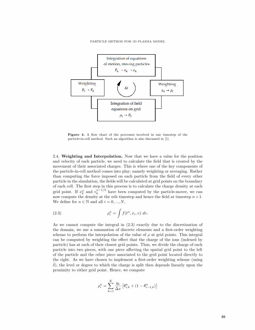
Figure 4. A flow chart of the processes involved in one timestep of the

particle-in-cell method. Such an algorithm is also discussed in [1].

2.4. Weighting and Interpolation. Now that we have a value for the positionand velocity of each particle, we need to calculate the field that is created by themovement of their associated charges. This is where one of the key components ofthe particle-in-cell method comes into play; namely weighting or averaging. Ratherthan computing the force imposed on each particle from the field of every otherparticle in the simulation, the fields will be calculated at grid points on the boundaryof each cell. The first step in this process is to calculate the charge density at eachgrid point. If xnk and v

n−1/2k have been computed by the particle-mover, we can

now compute the density at the nth timestep and hence the field at timestep n+ 1.We define for n ∈ N and all i = 0, ..., N ,

(2.3) ρni =∫f(tn, xi, v) dv.

As we cannot compute the integral in (2.3) exactly due to the discretization ofthe domain, we use a summation of discrete elements and a first-order weightingscheme to perform the interpolation of the value of ρ at grid points. This integralcan be computed by weighting the effect that the charge of the ions (indexed byparticle) has at each of their closest grid points. Thus, we divide the charge of eachparticle into two pieces, with one piece affecting the spatial grid point to the leftof the particle and the other piece associated to the grid point located directly tothe right. As we have chosen to implement a first-order weighting scheme (usingδ), the level or degree to which the charge is split then depends linearly upon theproximity to either grid point. Hence, we compute

ρni =K∑k=1

qk∆x

[θni,k + (1− θni−1,k)

]

89

D. BREWER

where the proportion of charge θni,k ∈ [0, 1] is given by the first-order weightingfunction

(2.4) θni,k = δ(xi − xnk )

and δ is defined by (2.2). This allows us to average the charge over all particlesand determine the density at spatial grid points (see Figure 3).

Though it is not immediately clear at present, it will be advantageous for uslater to utilize the function

(2.5) ψ(t, x) =∫

(1 + v)f(t, x, v) dv.

Further, we will denote the value of this function at grid points by ψni = ψ(tn, xi).Then, a similar weighting scheme can be utilized to compute these values from qkand vnk , namely

ψni =K∑k=1

qk∆x

(1 + vnk )[θni,k + (1− θni−1,k)

].

Once ρni and ψni have been computed, we define Bn+1i using a finite-difference

method to solve the field equation of (1.5), which depends upon knowledge of thesequantities. At this stage of the process, many options are available to computethe field values. As we will discuss in greater detail within the next section, themethod we have chosen utilizes an explicit, higher-order finite-difference scheme tocompute Bn+1

i for i = 0, ..., N .Finally, after the values of the field have been determined at grid points by Bn+1

i ,we must use them to determine the force on each particle at timestep (n + 1) sothat the particles can then be moved. However, particle quantities such as positionand momentum need not reside at gripoints and hence we need a similar weightingprocedure to generate forces “at the particle” from field values at meshpoints. Aspreviously mentioned, this is done by linear interpolation, or more precisely byusing

Fn+1k =

N∑i=1

(θni,k ·Bn+1

i + (1− θni,k) ·Bn+1i+1

)where θni,k ∈ [0, 1] is determined by the proximity of the particle’s position to theith spatial grid point using (2.4). The process may then continue by advancing theparticle positions and velocities, xnk and v

n−1/2k , to the next timestep, using the

particle-mover to compute vn+1/2k and then xn+1

k . A visualization of the sequenceof calculations for each timestep is shown in Figure 4.

2.5. Finite-Difference Methods and Lax-Wendroff. Though the particle methodis utilized to approximate the number density that satisfies the Vlasov equation of(1.5), we must still compute the values of B in the field equation. To do so weutilize a traditional finite-difference method. An introductory summary of suchmethods can be found in [11]. Assuming the values of Bni are known for everyi = 0, ..., N and some n ∈ N, we attempt to find the values of B at timestep(n+ 1), namely Bn+1

i . Applying the most elementary of these approximations, theone-sided forward-difference method, to the space and time derivatives in the fieldequation of (1.5):

∂tB + ∂xB = ρ,

90


we arrive atBn+1i −Bni

∆t+Bni+1 −Bni

∆x= ρni .

Therefore, the value of Bn+1i depends upon values of Bn at exactly two other grid

points, Bni and Bni+1. Since we are looking to find the value for B at the nexttimestep, we solve for Bn+1

i which yields

Bn+1i =

(1 +

∆t∆x

)Bni −

∆t∆x

Bni+1 + ∆tρni .

The forward-difference method is easy to implement since it is explicit in time;that is, it calculates values for timestep (n + 1) from known values via a finite-difference approximation at the nth timestep. Unfortunately, this method is knownto be numerically unstable. Additionally, it is well known that the error term of thisapproximation is only first order. To find a more accurate and stable approximationscheme, we look to a higher-order method.

What we desire is a method that incorporates the ease and expense of an ex-plicit forward-difference method, yet possesses better accuracy and stability prop-erties. Intuitively, since the error terms are calculated from the difference of theapproximations using a Taylor series, it would make sense to derive a higher-orderapproximation starting from the first few terms of the Taylor expansion, therebyreducing the error term. The so-called Lax-Wendroff method does just this. Itbegins with a Taylor series expansion over one timestep and converts each of theterms in the approximation to a different, but equivalent, form that contains notime derivatives. Using an idea similar to this, we expand the field B in time tofind

(2.6) B(t+ ∆t, x) = B(t, x) + ∆t · ∂tB(t, x) +(∆t)2

2∂ttB(t, x) +O(∆t3).

From the field equation, we know

∂tB = ρ− ∂xB.Hence, we can remove time derivatives of B, and therefore the need to know valuesof B at later timesteps, by replacing them with spatial derivatives of B and valuesof ρ. For the second-order term in the expansion, we need to find the second timederivative of B, and again the field equation yields

∂ttB = ∂tρ− ∂t(∂xB) = ∂tρ− ∂x(ρ− ∂xB) = ∂tρ− ∂xρ+ ∂xxB.

If we assume the particle distribution is periodic in v or possesses compact v-support, we can use the Vlasov equation of (1.5) to represent ∂tρ − ∂xρ withouttime derivatives as

∂tρ− ∂xρ =∫

(∂tf − ∂xf) dv

=∫

(∂tf + v∂xf − (1 + v)∂xf) dv

= −∫∂v(Bf) dv −

∫(1 + v)∂xf dv

= −∂x∫

(1 + v)f dv

= −∂xψ.

91

D. BREWER

Here∫∂vf dv = 0 due to the assumption of compact velocity support or periodicity

in v. Recall ψ was defined earlier in (2.5), and we can now see that this function isuseful in representing ∂ttB without time derivatives as

∂ttB = −∂xψ + ∂xxB.

Using these terms in the Taylor series expansion (2.6), we find

B(t+ ∆t, x) = B(t, x) + ∆t(ρ(t, x)− ∂xB(t, x))

+(∆t)2

2(∂xxB(t, x)− ∂xψ(t, x)) +O(∆t)3

(2.7)

Notice that the truncation of this approximation is accurate up to order (∆t)3.From this expression, we can apply central-difference approximations to the spatialderivatives. In general, such an approximation can be derived by subtracting theTaylor series expansions for an arbitrary smooth function µ(x) about the pointsx+ ∆x and x−∆x, with ∆x > 0. Doing this yields

µ(x+ ∆x)− µ(x−∆x) = 2∆xµ′(x) +23!

(∆x)3µ′′′(x) + · · ·

or µ′(x) ≈ µ(x+∆x)−µ(x−∆x)2∆x with an error term of order (∆x)2, assuming µ′′′ is

bounded. A second-derivative central-difference approximation can also be derivedfrom the Taylor series by adding the function values of µ at x + ∆x to those atx−∆x to find

µ(x+ ∆x) + µ(x−∆x) = 2µ(x) + (∆x)2µ′′(x) +24!

(∆x)4µ(4)(x) + · · ·

or µ′′(x) ≈ µ(x+∆x)−2µ(x)+µ(x−∆x)(∆x)2 with an error term of order (∆x)2, assuming

µ(4) is bounded. Discretizing these difference formulas and applying them to the∂xB, ∂xψ, and ∂xxB terms, we have

(2.8)

∂xB(tn, xi) ≈Bni+1 −Bni−1

2∆x

∂xψ(tn, xi) ≈ψni+1 − ψni−1

2∆x

∂xxB(tn, xi) ≈Bni+1 − 2Bni +Bni−1

(∆x)2.

Assuming the bounds on higher derivatives above, the approximations in (2.8) areaccurate up to order (∆x)2.

Finally, we use the approximations (2.8) in (2.7) evaluated at t = tn and x = xito find our explicit, second-order finite-difference approximation of the field

Bn+1i = Bni + ∆t

(ρni −

Bni+1 −Bni−1

2∆x

)+

(∆t)2

2

(Bni+1 − 2Bni +Bni−1

(∆x)2−ψni+1 − ψni−1

2∆x

)or grouping terms,

Bn+1i =

(1−

(∆t∆x

)2)Bni + ∆tρni −

(∆t)2

4∆x(ψni+1 − ψni−1)

− ∆t2∆x

[(1− ∆t

∆x)Bni+1 − (1 +

∆t∆x

)Bni−1

].

(2.9)

92


This is the finite-difference equation in its final form that is implemented in theprogram to compute the field at the next timestep, for every i = 1, ..., N − 1 andn = 0, ..., P − 1. The only stipulation to the ensure the stability of this methodis a well-known statement called the Courant-Friedrichs-Lewy (or CFL, cf. [12])condition which states that we must choose ∆t and ∆x in order to satisfy ν∆t

∆x ≤ 1,where ν is the characteristic speed of the signals generated by the field B(t, x). Inour case, ν is the speed of light, which has been normalized to 1. Since the fieldequation tells us that such characteristics move to the right with speed ν = 1, weneed only choose ∆t ≤ ∆x to ensure stability of the method.

Hence, in our particle code, we employ a variant of the Lax-Wendroff scheme:an explicit one-step method which, when solved for at timestep (n+ 1), is given by(2.9). As shown above this method increases the order of accuracy (to order (∆x)2)of the one-sided, explicit method and does not require the extra computations thatare needed to utilize an implicit method. In this vein, we now turn our attention togauging the accuracy of the entire particle-in-cell method used to model the system.

2.6. Accuracy and a Conserved Quantity. Since the particle method utilizesa number of mathematical approximations for the differential equations, it can bedifficult to determine a precise order of accuracy analytically, though some erroranalysis of (1.2) has been performed [18], [8], [2]. Often a good heuristic for mea-suring accuracy is the extent to which the PIC method preserves the value of theconserved energy. We note, however, that in some cases secular changes in suchconserved quantities can be observed during PIC simulations, for example due toself-heating [1], [10]. In our case, we can derive a conserved, energy-like quantity for(1.5). Though this quantity technically does not represent the energy of a physicalsystem, we will still refer to it as the energy for (1.5). As we will see this quantityis an invariant of the system and is similar to the conserved energy of (1.1) in thatit contains a velocity moment (though first-order instead of second) in the kineticportion and the square of the field in the potential portion.

The specific method we will employ is quite simple: the simulation value ofthe energy is computed at each timestep and measured against its initial valueto see how well it is conserved throughout. Specifically, this quantity is found bycomputing the Hamiltonian of the system (1.5). To derive a formula for this, wemust start by making a few assumptions. Namely, we assume that the particledistribution tends to zero at infinity; i.e., f(t, x, v)→ 0 as |x| → ∞ or |v| → ∞ forevery t > 0. In addition, we assume that a similar statement holds for the field;i.e., B(t, x) → 0 as |x| → ∞ for every t > 0. Assumptions of compact support orperiodicity (which we shall implement later) for these functions would be sufficientas well.

Next, we derive the corresponding conservation law. To this end, we define

E(t) =12

∫B(t, x)2 dx−

∫∫vf(t, x, v) dv dx.

Taking the time derivative, integrating by parts, and using (1.5) with the afore-mentioned boundary or support assumption, it is a straightforward calculation toshow that E ′(t) = 0. Hence, E(t) is constant and therefore we write

E(t) = E :=12

∫B0(x)2 dx−

∫∫vf0(x, v) dv dx

93

D. BREWER

for every t ≥ 0. Here, the first term of E represents the potential energy in thesystem, while the second represents a corresponding kinetic energy term. Noticethat each possesses an integral that must be approximated numerically. Thus,instead of tracking E throughout the particle simulation, we define a discretizedanalogue which we deem the simulation energy, namely

(2.10) E(t) =12

N∑i=1

(Bni )2 ·∆x−K∑k=1

vnk · qk

where t = n ·∆t. Here, vnk is computed by stepping forward in time by ∆t/2 fromthe value of vn−1/2

k in the same way that we initially push back v0k. Within the

simulations of the next section, we will use this quantity to provide some measure asto the effectiveness of our computations. For instance, if we find that E has changedby 3% at the stopping time, then we can generally assume that our computationof the solution is within 3% of its true value. In addition to this, we will verify thespatial accuracy of the simulations in a later section by computing a derived steadystate.

3. Boundary Conditions and Particle Method Testing

In order to construct and implement any numerical method for this problem,the initial state of the plasma (via its initial particle distribution f0 and initial fieldB0) must be known in advance. Additionally, the aforementioned finite-differencemethods require boundary conditions in order to solve the corresponding equationsnear the boundary of the spatial grid. Thus, we now discuss the variety of optionsavailable for the boundary data.

3.1. Boundary Conditions. Since it is important for the equations to modela variety of situations, and the simulations require knowledge of the behavior ofparticles at the boundaries of the spatial domain (recall that the velocity domainis unconstrained throughout the simulation), we consider many different boundaryconditions (BCs). The most often used of these in such simulations are:

(1) Periodic boundary conditions(2) Absorbing boundary conditions(3) Reflective boundary conditions.

A physical picture of these conditions is displayed in Figure 5. The first variety ofboundary condition models the motion of the plasma when moving along a periodicstructure or within a periodic medium. When a particle in the simulation reachesthe spatial boundary, its position is reinitialized to emanate from the opposingboundary wall by the exact amount from which it escaped the domain. Similarly,spatial periodicity is imposed on the field. Often the mathematical assumption ofperiodicity is made in order to study this phenomena in different geometries such ascrystals or torii, which possess the interesting property of repeating their inherentstructure.

The second condition, namely absorption of the charge at the boundary, modelsthe situation in which particles that leave a specific spatial region become separatedfrom the remaining plasma. When a particle in the simulation reaches the bound-ary, its charge is identically set to zero, thereby “absorbing” its ionic attributes atthe boundary wall. Once a particle exits through one side of the mesh boundary,it no longer affects the remaining particles, thereby leading to a dissipation of the

94


(a) Periodic BCs

(b) Absorbing BCs

(c) Reflective BCs

Figure 5. Graphical representations of different boundary conditions for theplasma described by (1.5). Vertical lines represent spatial boundaries, solid

horizontal lines represent particle trajectories within the spatial domain, and

dashed horizontal lines represent these trajectories outside of the domain. Thedistance a denotes the effect that the particle paths encounter upon reaching

the boundary.

energy. Thus, we naturally expect E to decrease significantly during any simula-tion that utilizes absorbing boundary conditions. Additionally, Dirichlet boundaryconditions are utilized for the field.

The third condition, in which particles are reflected (and therefore not allowedto escape the simulation), is perhaps the most complicated boundary condition.In this scenario, we assume that a barrier exists at the spatial boundary thatreflects particles back into the domain of interest. We are careful to note herethat the type of reflection assumed in the simulation is that of a perfectly elasticcollision. More specifically, it is assumed that upon colliding with the barrier at theboundary, a particle’s inherent properties remain unchanged other than by alteringits direction; that is, we say that no exchange of momentum takes place whenthe particle comes in contact with the boundary. Instead, it is perfectly reflectedback into the domain with a velocity of equal magnitude but opposite direction.Again, Dirichlet boundary conditions are implemented for the field computations.Since (1.5) is a hyperbolic system, we must also choose the initial data for Bto be compatible with the imposed boundary conditions. Hence, we shall choosethe initial field B0(x) later to satisfy either periodicity or the Dirichlet boundaryconditions, as well.

3.2. Verification and Testing. In order to test the previously described particlemethod using a known steady state solution, we follow the explicit example of [14].We utilize two species of ions: positive charges with density f+ and electrons withdensity f−. In this situation the steady charge density is determined using the sum

95

D. BREWER

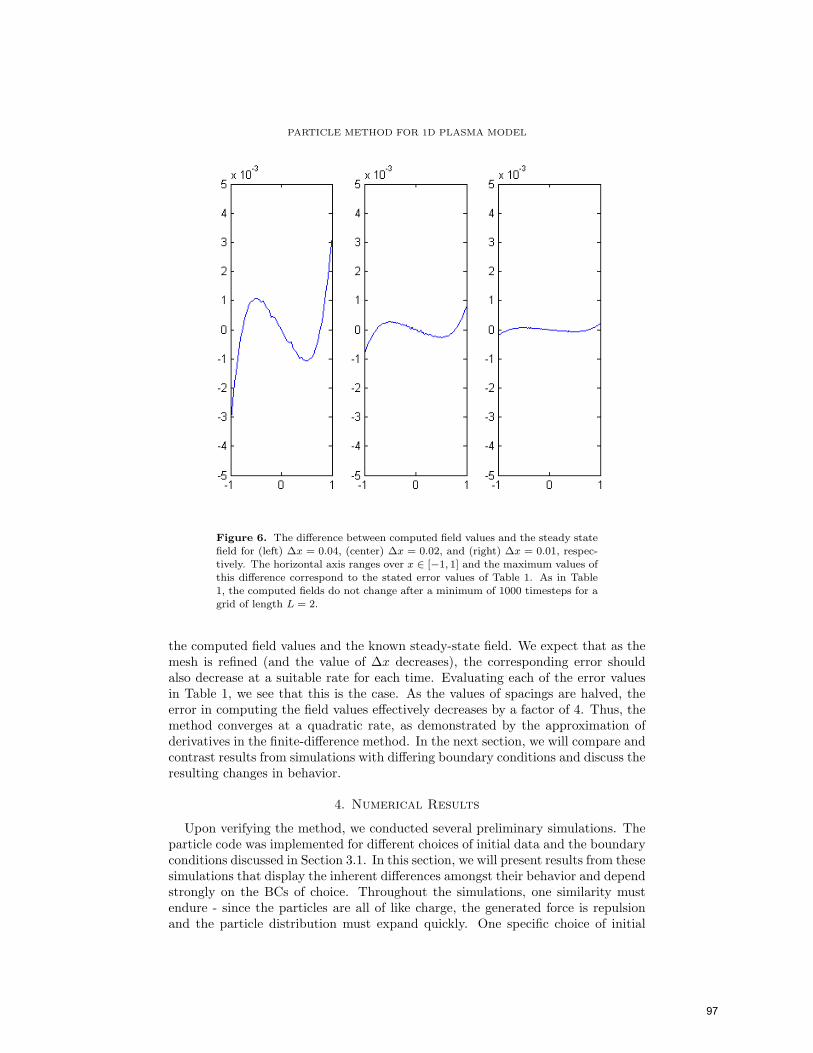
∆x supi |Bni −B(xi)| supi |Bni |0.04 3.20× 10−3 0.858

0.02 7.99× 10−4 0.858

0.01 2.00× 10−4 0.858Table 1. Error of the field for steady state solution. Here Bn

i is the computed

field and B(xi) is the known steady state solution evaluated at spatial grid

points. The error values in the table are identical over a minimum of 1000timesteps for a spatial grid of [−1, 1]

of the particle distributions by

ρ(x) =∫ (

f+(x, v)− f−(x, v))dv.

We let the electron distribution be defined as a function of the Hamiltonian

f−(x, v) = F(

12|v|2 + U(x)

),

where

F(e) ={−e if e ≤ 00 if e > 0

andU(x) = −1

2(1− x2)3χ[−1,1](x)

is the potential for the steady field B(x). Here,

χA(x) =

{1, if x ∈ A0, if x 6∈ A

is the indicator function for the set A. From U(x) the time-independent field iscalculated by

B(x) = U ′(x) = 3x(1− x2)2χ[−1,1](x).Additionally, the steady charge density can be found by calculating the derivativeof the field

ρ(x) = B′(x) = 3(1− x2)(1− 5x2)χ[−1,1](x).Therefore, the distribution of positive charge is determined by ρ and f− as∫

f+(x, v) dv = ρ(x) +∫f−(x, v) dv

whence we may take

f+(x, v) =(

3(1− x2)(1− 5x2) +23

(1− x2)92

)χ[−1,1](x)δ(v)

where δ is the Dirac delta function.Using these functions, the method was implemented for several choices of ∆x,∆v,

and ∆t with periodic boundary conditions in order to ensure convergence to thecorrect steady state solution. Table 1 summarizes the results of these runs, listingthe error found by calculating the difference between the known steady field solutionand the computed field at every timestep. Figure 6 displays a comparison between

96


Figure 6. The difference between computed field values and the steady state

field for (left) ∆x = 0.04, (center) ∆x = 0.02, and (right) ∆x = 0.01, respec-

tively. The horizontal axis ranges over x ∈ [−1, 1] and the maximum values ofthis difference correspond to the stated error values of Table 1. As in Table

1, the computed fields do not change after a minimum of 1000 timesteps for a

grid of length L = 2.

the computed field values and the known steady-state field. We expect that as themesh is refined (and the value of ∆x decreases), the corresponding error shouldalso decrease at a suitable rate for each time. Evaluating each of the error valuesin Table 1, we see that this is the case. As the values of spacings are halved, theerror in computing the field values effectively decreases by a factor of 4. Thus, themethod converges at a quadratic rate, as demonstrated by the approximation ofderivatives in the finite-difference method. In the next section, we will compare andcontrast results from simulations with differing boundary conditions and discuss theresulting changes in behavior.

4. Numerical Results

Upon verifying the method, we conducted several preliminary simulations. Theparticle code was implemented for different choices of initial data and the boundaryconditions discussed in Section 3.1. In this section, we will present results from thesesimulations that display the inherent differences amongst their behavior and dependstrongly on the BCs of choice. Throughout the simulations, one similarity mustendure - since the particles are all of like charge, the generated force is repulsionand the particle distribution must expand quickly. One specific choice of initial

97

D. BREWER

0 10 20 30 40 50t0.110

0.115

0.120

0.125

0.130

0.135

0.140

0.145

0.150EHtL

(a) A graph of E(t) for t ∈ [0, 50]. Here,

we have taken ∆ := ∆x = ∆v = ∆t =0.01 and used the initial data of (IC) with

periodic BCs. Notice that the value of E is

increasing very slowly over time, changingby only 4% over 5000 timesteps.

5 10 15 20 25 30t0

2

4

6

8

10EHtL

(b) A graph of the

KXk=1

vnk qk for t ∈ [0, 10].

Here, we have taken ∆ = 0.01 and used the

initial data of (IC2) with absorbing BCs.

Notice that the values are decreasing dras-tically over time, thus demonstrating the

dissipation due to absorption of charge atthe spatial boundary.

Figure 7. The change in the energy over time for periodic and absorbing BCs

data represents a smooth, compactly-supported distribution of ions in the systemthat quickly decays to zero. The initial field is taken to be sinusodial in order torepresent the wave-like behavior of such physical phenomena. We utilize the phasespace (x, v) ∈ [−1, 1]× [−1, 1] and define the functions

(IC)

f0(x, v) = (1− 4x2)2(1− 4v2)2χ[− 1

2 ,12 ](x)χ[− 1

2 ,12 ](v)

B0(x) =12

sin(2πx)χ[−1,1](x).

With these initial conditions, the energy is easily calculated by subtracting∫∫vf0(x, v) dv dx = 0

from the square norm of the field

12

∫B0(x)2 dx =

12· 1

4= 0.125.

Here, the kinetic portion is zero due to the even symmetry of the initial chargedistribution, and we find that E(0) = 0.125.

Beginning with the test runs of the previous section, a simulation of (1.5) as-suming initial conditions (IC) and periodic boundary conditions was conducted for∆ = ∆t = ∆x = ∆v = 0.01. Figure 7a shows E in the computational domain fortimes 0 ≤ t ≤ 50. As previously mentioned, the deviation of this quantity fromits initial (and conserved) value is seen as a good measure of the accuracy of themethod over time. In this case, the values range between 0.12500, initially, and0.13011, at time t = 50. In order to measure this difference, we compute the rela-tive change in values of E over time. Table 2 summarizes the results of these runs,listing the values of the relative change as the mesh values are decreased. This

98


∆ t = 2 t = 4 t = 6 t = 8 t = 100.10 1.36× 10−2 3.15× 10−2 6.10× 10−2 1.02× 10−1 1.58× 10−1

0.05 5.86× 10−3 1.04× 10−2 1.81× 10−2 2.89× 10−2 4.27× 10−2

0.025 2.62× 10−3 3.73× 10−3 5.70× 10−3 8.46× 10−3 1.20× 10−2

0.0125 1.22× 10−3 1.48× 10−3 1.98× 10−3 2.68× 10−3 3.58× 10−3

Table 2. The relative error of the simulation energy RE(t). Here, we take

∆ = ∆t = ∆x = ∆v and use periodic boundary conditions. The initial value

E(0) = 0.125 is identical to E, and hence RE(0) = 0, for every choice of meshor grid size.

quantity is found by calculating the difference between the known conserved valueand the computed simulation value at every timestep and dividing by E , i.e.

RE(t) =E(t)− E(0)E(0)

.

For instance, from Figure 7a we can see that the relative change for ∆x = ∆v =∆t = 0.01 at t = 50 is computed to be

RE(50) =E(50)− E(0)E(0)

=0.13011− 0.125

0.125≈ 0.0409 = 4.09%.

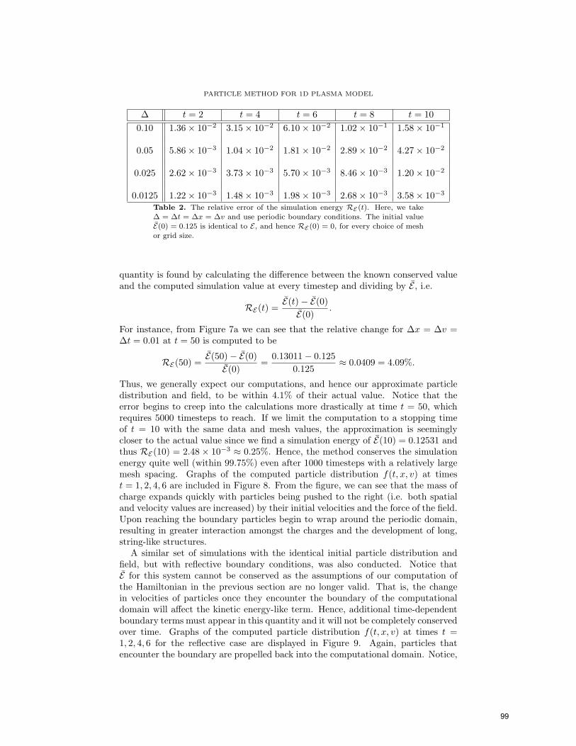
Thus, we generally expect our computations, and hence our approximate particledistribution and field, to be within 4.1% of their actual value. Notice that theerror begins to creep into the calculations more drastically at time t = 50, whichrequires 5000 timesteps to reach. If we limit the computation to a stopping timeof t = 10 with the same data and mesh values, the approximation is seeminglycloser to the actual value since we find a simulation energy of E(10) = 0.12531 andthus RE(10) = 2.48 × 10−3 ≈ 0.25%. Hence, the method conserves the simulationenergy quite well (within 99.75%) even after 1000 timesteps with a relatively largemesh spacing. Graphs of the computed particle distribution f(t, x, v) at timest = 1, 2, 4, 6 are included in Figure 8. From the figure, we can see that the mass ofcharge expands quickly with particles being pushed to the right (i.e. both spatialand velocity values are increased) by their initial velocities and the force of the field.Upon reaching the boundary particles begin to wrap around the periodic domain,resulting in greater interaction amongst the charges and the development of long,string-like structures.

A similar set of simulations with the identical initial particle distribution andfield, but with reflective boundary conditions, was also conducted. Notice thatE for this system cannot be conserved as the assumptions of our computation ofthe Hamiltonian in the previous section are no longer valid. That is, the changein velocities of particles once they encounter the boundary of the computationaldomain will affect the kinetic energy-like term. Hence, additional time-dependentboundary terms must appear in this quantity and it will not be completely conservedover time. Graphs of the computed particle distribution f(t, x, v) at times t =1, 2, 4, 6 for the reflective case are displayed in Figure 9. Again, particles thatencounter the boundary are propelled back into the computational domain. Notice,

99

D. BREWER

(a) Time t = 0 (b) Time t = 1

(c) Time t = 2 (d) Time t = 4

Figure 8. The particle distribution with periodic BCs using (IC) at times

t = 0, 1, 2, 4. Notice that the values of the velocities of particles (y-axis) mayincrease outside of the original domain of [−1, 1], but spatial values (x-axis)

do not.

however, at time t = 2 a group of particles that attempts to leave the region ispushed back into the domain with identical spatial values but negative velocities,in contrast to those of the periodic case that maintain their velocity values but arespatially transported to the other end of the x interval.

Finally, we implemented the method to generate simulations with absorbingboundary conditions and the following initial data:

(IC2)

f0(x, v) = (1− 4x2)2(1− 4|v − 0.3|2)2χ[− 1

2 ,12 ](x)χ[− 1

2 ,12 ](|v − 0.3|)

B0(x) =12

sin(2πx)χ[−1,1](x).

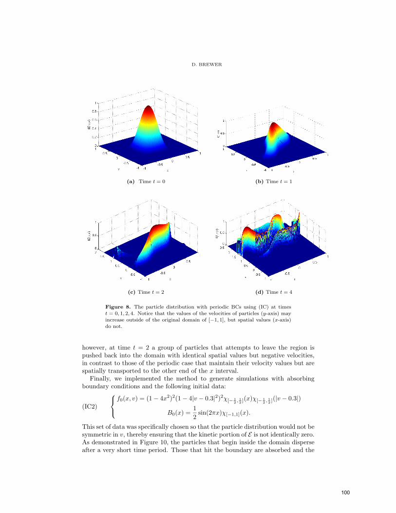
This set of data was specifically chosen so that the particle distribution would not besymmetric in v, thereby ensuring that the kinetic portion of E is not identically zero.As demonstrated in Figure 10, the particles that begin inside the domain disperseafter a very short time period. Those that hit the boundary are absorbed and the

100




Figure 9. The particle distribution with reflective BCs using (IC2) at times

t = 0, 1, 2, 4

charge in the system quickly dissipates. Particles that begin with small velocitiesand are initially positioned far from the boundary remain in the simulation butcarry very little charge. Eventually, however, the force of the imposed field mustpush them far enough to the right that they interact with the boundary and areabsorbed. After time t = 5, no charged particles remain, and the system ceases tochange. Similar to Figure 7a, a graph of E(t) is displayed in Figure 7b. Notice thatthis quantity quickly decays as the particles are absorbed at the boundaries, andhence kinetic energy is lost in the system. As in the case of reflective boundaryconditions, E cannot be conserved as the absorbing boundary alters the computationof the Hamiltonian in Section 3.

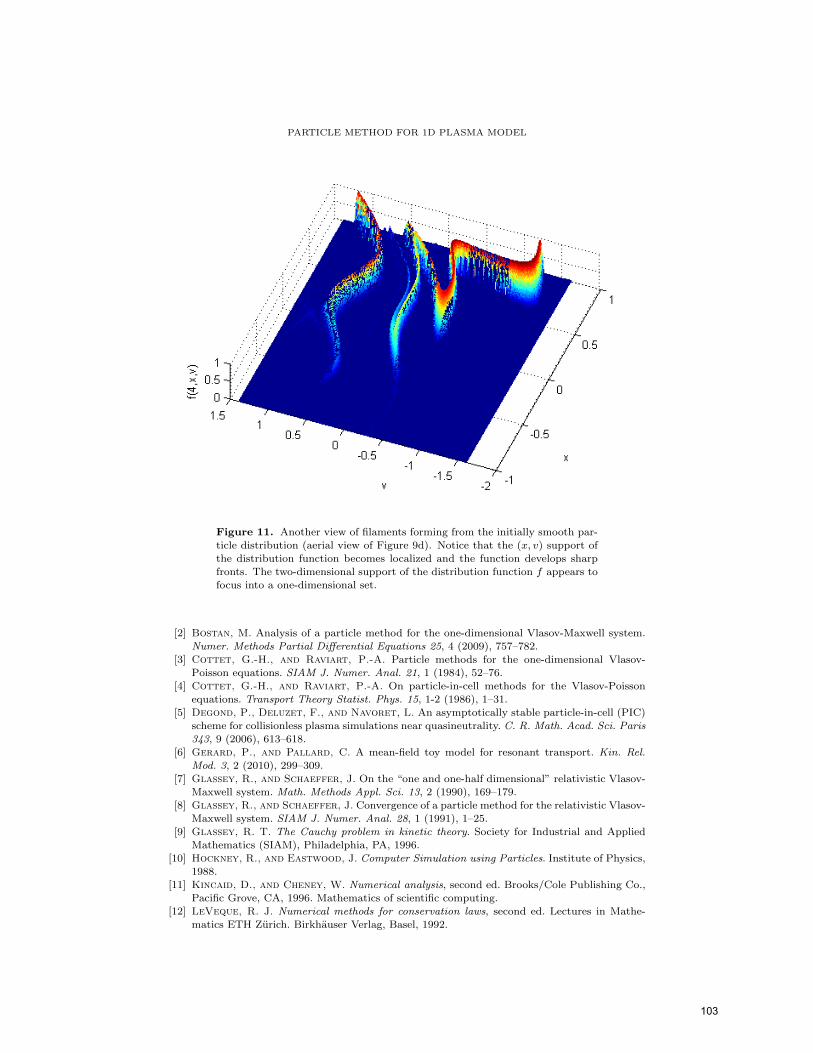
Regardless of the boundary conditions utilized, the particle distribution seemsto develop filaments, or localized “string-like” pieces rather quickly (see Fig 11).These structures occur along curves in phase space at which the derivatives off(t, x, v) grow large. In each case this seems to occur even before additional particleinteraction arises from the imposed boundary conditions and leads one to believethat it is possible for discontinuities in phase space to occur even from smooth

101

D. BREWER



Figure 10. The particle distribution with absorbing BCs using (IC2) at times

t = 0, 2, 4, 5

initial data such as (IC) and (IC2). As one can see from Fig 11, the two-dimensionalsupport of the distribution function f appears to focus into a one-dimensional set.Such an occurrence of discontinuities for (1.5) would exist in sharp contrast tosimulations of (1.2) in which solutions remain smooth if they begin with a smoothinitial distribution (cf. [14]). A proof of this regularity result has even been obtainedfor the much more difficult three-dimensional analogue of (1.2) in [16]. Such aquestion regarding the loss of regularity of solutions in the case of a transport field,i.e. for (1.5), or for the full Vlasov-Maxwell system (1.1), remains unanswered.However, some limited progress has been made in [13] for (1.5). It is our hope thatour method and results will both lead to the development of new intuition and serveas the impetus for further study of the properties of solutions to kinetic equationswhen coupled to a transported or, more generally an electromagnetic, field.

References

[1] Birdsall, C., and Langdon, A. Plasma Physics Via Computer Simulation. Institute of

Physics, Series in Plasma Physics. Taylor and Francis, New York, NY, 1991.

102


Figure 11. Another view of filaments forming from the initially smooth par-

ticle distribution (aerial view of Figure 9d). Notice that the (x, v) support of

the distribution function becomes localized and the function develops sharpfronts. The two-dimensional support of the distribution function f appears to

focus into a one-dimensional set.

[2] Bostan, M. Analysis of a particle method for the one-dimensional Vlasov-Maxwell system.

Numer. Methods Partial Differential Equations 25, 4 (2009), 757–782.[3] Cottet, G.-H., and Raviart, P.-A. Particle methods for the one-dimensional Vlasov-

Poisson equations. SIAM J. Numer. Anal. 21, 1 (1984), 52–76.[4] Cottet, G.-H., and Raviart, P.-A. On particle-in-cell methods for the Vlasov-Poisson

equations. Transport Theory Statist. Phys. 15, 1-2 (1986), 1–31.

[5] Degond, P., Deluzet, F., and Navoret, L. An asymptotically stable particle-in-cell (PIC)scheme for collisionless plasma simulations near quasineutrality. C. R. Math. Acad. Sci. Paris

343, 9 (2006), 613–618.

[6] Gerard, P., and Pallard, C. A mean-field toy model for resonant transport. Kin. Rel.Mod. 3, 2 (2010), 299–309.

[7] Glassey, R., and Schaeffer, J. On the “one and one-half dimensional” relativistic Vlasov-

Maxwell system. Math. Methods Appl. Sci. 13, 2 (1990), 169–179.[8] Glassey, R., and Schaeffer, J. Convergence of a particle method for the relativistic Vlasov-

Maxwell system. SIAM J. Numer. Anal. 28, 1 (1991), 1–25.

[9] Glassey, R. T. The Cauchy problem in kinetic theory. Society for Industrial and AppliedMathematics (SIAM), Philadelphia, PA, 1996.

[10] Hockney, R., and Eastwood, J. Computer Simulation using Particles. Institute of Physics,

1988.[11] Kincaid, D., and Cheney, W. Numerical analysis, second ed. Brooks/Cole Publishing Co.,

Pacific Grove, CA, 1996. Mathematics of scientific computing.[12] LeVeque, R. J. Numerical methods for conservation laws, second ed. Lectures in Mathe-

matics ETH Zurich. Birkhauser Verlag, Basel, 1992.

103

D. BREWER

[13] Nguyen, C., Anderson, J., and Pankavich, S. A one-dimensional kinetic model of plasma

dynamics with a transport field. submitted to SIAM Journal on Mathematical Analysis

(2010).[14] Pankavich, S. A particle method for a collisionless plasma with infinite mass. submitted to

Math. Comp. Sim. (2010).

[15] Schaeffer, J. The classical limit of the relativistic Vlasov-Maxwell system. Comm. Math.Phys. 104, 3 (1986), 403–421.

[16] Schaeffer, J. Global existence of smooth solutions to the Vlasov-Poisson system in three

dimensions. Comm. Partial Differential Equations 16, 8-9 (1991), 1313–1335.[17] van Kampen, N., and Felderhof, B. Theoretical Methods in Plasma Physics. Wiley, New

York, NY, 1967.

[18] Victory, Jr., H. D., Tucker, G., and Ganguly, K. The convergence analysis of fullydiscretized particle methods for solving Vlasov-Poisson systems. SIAM J. Numer. Anal. 28,

4 (1991), 955–989.

Department of Mathematics, University of Texas at Arlington, 411 S NeddermanDrive, Arlington, Texas 76019

E-mail address: [email protected]

104

computational methods for a one-dimensional plasma - siam

Documents