computational mechanics research and support for ... mechanics research and support for aerodynamics...

Computational Mechanics Research and Support

for Aerodynamics and Hydraulics at TFHRC

ANL/ESD/13-5

Year 3 Quarter 2 Progress Report

Disclaimer This report was prepared as an account of work sponsored by an agency of the United States Government. Neither the United States Government nor any agency thereof, nor UChicago Argonne, LLC, nor any of their employees or officers, makes any warranty, express or implied, or assumes any legal liability or responsibility for the accuracy, completeness, or usefulness of any information, apparatus, product, or process disclosed, or represents that its use would not infringe privately owned rights. Reference herein to any specific commercial product, process, or service by trade name, trademark, manufacturer, or otherwise, does not necessarily constitute or imply its endorsement, recommendation, or favoring by the United States Government or any agency thereof. The views and opinions of document authors expressed herein do not necessarily state or reflect those of the United States Government or any agency thereof, Argonne National Laboratory, or UChicago Argonne, LLC.

Availability of This Report This report is available, at no cost, at http://www.osti.gov/bridge. It is also available on paper to the U.S. Department of Energy and its contractors, for a processing fee, from:

U.S. Department of Energy Office of Scientific and Technical Information P.O. Box 62 Oak Ridge, TN 37831-0062 phone (865) 576-8401 fax (865) 576-5728

[email protected]

About Argonne National Laboratory

Argonne is a U.S. Department of Energy laboratory managed by UChicago Argonne, LLC

under contract DE-AC02-06CH11357. The Laboratory’s main facility is outside Chicago,

at 9700 South Cass Avenue, Argonne, Illinois 60439. For information about Argonne

and its pioneering science and technology programs, see www.anl.gov.

Computational Mechanics Research and Support for Aerodynamics and Hydraulics at TFHRC, Year 3 Quarter 2 Progress Report

by S.A. Lottes1, C. Bojanowski1, J. Shen2, and Z. Xie2 1 Transportation Research and Analysis Computing Center (TRACC) Energy Systems Division, Argonne National Laboratory 2 Turner-Fairbank Highway Research Center submitted to Kornel Kerenyi1 and Harold Bosch1 1 Turner-Fairbank Highway Research Center July 2013

ANL/ESD/13-5

TRACC/TFHRC Y3Q2 Page 3

Table of Contents

1. Introduction and Objectives ................................................................................................................. 9

1.1. Hydraulics Modeling and Analysis Summary ................................................................................. 10

1.2. Wind Engineering Modeling and Analysis Summary ..................................................................... 10

1.3. Weathering Steel Modeling and Analysis Summary ...................................................................... 10

1.4. Technology Transfer and Facility and User Support ...................................................................... 10

2. Hydraulics Modeling and Analysis ...................................................................................................... 11

2.1. Onset of Rip-Rap Motion using STAR-CCM+ Coupled with LS-DYNA............................................. 11

2.2. Flume Design Modeling at TFHRC .................................................................................................. 13

3. Wind Engineering Modeling and Analysis........................................................................................... 21

3.1. Analysis of Sign Vibration Due to Passing Trucks ........................................................................... 21

3.1.1. Literature Review ................................................................................................................ 21

3.1.2. Results of CFD Analysis ....................................................................................................... 24

3.1.3. Results of Structural Analysis .............................................................................................. 34

3.1.4. Summary ............................................................................................................................. 40

3.1.5. References .......................................................................................................................... 41

3.2. Wind Tunnel Model Comparison with Laboratory Experiments ................................................... 42

3.2.1. Replacement of Fan Model with Specified Velocity Inlet and Pressure Outlets ................ 42

3.2.2. Determination of Inlet Velocity for Chamber Section ........................................................ 44

3.2.3. Comparison of Laboratory Measurements and CFD Results .............................................. 45

4. Weathering Steel Truck Spray Modeling and Analysis ....................................................................... 52

4.1. Topics for Future Analysis .............................................................................................................. 52

5. Technology Transfer ........................................................................................................................... 55

6. TRACC Facility and User Support for TFHRC ....................................................................................... 57


List of Figures

Figure 2.1 Stages in the coupled simulation for water induced stone motion ........................................... 12

Figure 2.2 Problem with multiple remeshing without preserving geometrical features ........................... 12

Figure 2.3 Velocity distribution and VOF contour for wind tunnel transition profile: Case 1 .................... 13

Figure 2.4 Dimensions sketch for 25% reduction of vertical transition ...................................................... 14

Figure 2.5 Velocity magnitude contour without honey comb: case 2a ...................................................... 14

Figure 2.6 Velocity magnitude contour with honey comb: case 2b ........................................................... 14

Figure 2.7 Velocity magnitude contour with the changed position of pipe diffuser: case 2c .................... 15

Figure 2.8 Velocity magnitude contour without honeycomb: case 3a ....................................................... 15

Figure 2.9 Velocity magnitude contour with honeycomb: case 3b ............................................................ 15

Figure 2.10 Velocity magnitude contour with the changed position of pipe diffuser: case 3c .................. 15

Figure 2.11 Velocity magnitude contour and velocity vector: case 4a ....................................................... 16

Figure 2.12 Velocity magnitude contour, velocity vector and free water surface: case 4b ....................... 17

Figure 2.13 Velocity magnitude contour and velocity vector for shorter diffuser: case 4 ......................... 17

Figure 2.14 Velocity magnitude contour and velocity vector for spiral wall profile: Case 6a .................... 18

Figure 2.15 Velocity magnitude contour and velocity vector for spiral wall profile: case 6b .................... 18

Figure 2.16 Velocity magnitude contour and velocity vector for porous media cage diffuser: case 7 ...... 19

Figure 2.17 Domain for data selection in space.......................................................................................... 19

Figure 3.1 Shape of the impulse function assumed by Creamer et. al [1]. ................................................. 21

Figure 3.2 Typical truck induced gust pressure history by Cook et al. 1996 [3] ......................................... 23

Figure 3.3 Air flow past truck moving 60 mph and assumed air diversion by Desantis [5] ........................ 24

Figure 3.4 CFD model geometry with interfaces used in sliding mesh motion .......................................... 25

Figure 3.5 Trucks without and with over cab flow diverter or non-streamlined and streamlined ............ 25

Figure 3.6 Positions of the truck corresponding to the peaks in the pressure history ............................... 26


Figure 3.7 Pressure distribution on the sign surface at the time when local negative peaks occur .......... 27

Figure 3.8 Pressure history on the front panel of the sign for simulations with streamlined truck and

different velocities ...................................................................................................................................... 28

Figure 3.9 Pressure history on the front panel of the sign for simulations with non-streamlined truck and


Figure 3.10 Pressure history on the bottom panel of the sign for simulations with streamlined truck and


Figure 3.11 Pressure history on the bottom panel of the sign for simulations with non-streamlined truck

and different velocities ............................................................................................................................... 29

Figure 3.12 Dependency of the pressure on the truck speed .................................................................... 29

Figure 3.13 Pressure history on the front panel of the sign for simulations with non-streamlined truck

and different sign height ............................................................................................................................. 30

Figure 3.14 Pressure history on the bottom panel of the sign for simulations with non-streamlined truck

and different sign height ............................................................................................................................. 30

Figure 3.15 Dependency of the pressure on the sign height ...................................................................... 31

Figure 3.16 Geometry of the TFHRC sign and its location over the highway lanes .................................... 31

Figure 3.17 Worst case scenario analyzed - two trucks passing simultaneously under the sign ............... 32

Figure 3.18 Comparison of the pressure histories on the frontal panel due to different truck

configuration under the sign ...................................................................................................................... 32

Figure 3.19 Comparison of the pressure histories on the bottom panel due to different truck

configuration under the sign ...................................................................................................................... 33

Figure 3.20 Pressure history on the sign frontal panel due to 10 mph head wind and passage of a two

trucks under the sign .................................................................................................................................. 33

Figure 3.21 Pressure history on the sign bottom panel due to 10 mph head wind and passage of a two

trucks under the sign .................................................................................................................................. 34

Figure 3.22 Eigenvalues and eigenmodes for the TFHRC sign model ......................................................... 35

Figure 3.23 Free vibration history of the cantilever tip (left) in the X direction and (right) in the Z

direction due to gravity and forward force impulse (X direction) .............................................................. 36

Figure 3.24 FFT of the free vibration history of the cantilever tip (left) in the X direction (right) the Z

direction due to gravity and forward force impulse (X direction) .............................................................. 36


Figure 3.25 Free vibration history of the cantilever tip (left) in the Z direction and (right) in the X

direction due to gravity and pull down impulse (X direction) .................................................................... 37

Figure 3.26 FFT of the free vibration history of the cantilever tip (left) in the Z direction and (right) in the

X direction due to gravity and pull down force impulse (X direction) ........................................................ 37

Figure 3.27 Free vibration history of the cantilever tip (left) in the Z direction (right) in the X direction

due to truck passage ................................................................................................................................... 37

Figure 3.28 FFT of the free vibration history in the Z direction of the cantilever tip due to truck passage

.................................................................................................................................................................... 38

Figure 3.29 Vibration history of the cantilever tip in Z direction caused by passage of one truck ............ 38

Figure 3.30 Vibration history of the cantilever tip in Z direction caused by passage of three trucks (left)

no damping (right) 1% of critical damping.................................................................................................. 39

Figure 3.31 Typical pressure history acting on one element of front panel coming from combined load

from 20 trucks passing under the sign ........................................................................................................ 39

Figure 3.32 Vibration history of the cantilever tip in Z direction caused by passage of twenty trucks (left)

simulation without structural damping (right) with 1 % of critical damping ............................................. 40

Figure 3.33 Vibration history of the cantilever tip in Z direction caused by passage of six trucks and 10

mph head wind ........................................................................................................................................... 40

Figure 3.34 Zones in the fan section of the wind tunnel ............................................................................ 43

Figure 3.35 Portion of fan chamber showing inlet to wind tunnel in pink highlight .................................. 44

Figure 3.36 Portion of fan zone showing boundary between room and fan section in pink highlight ...... 44

Figure 3.37 CFD computed velocity vector field at the height of the laboratory measurements .............. 46

Figure 3.38 Vector field plotted from laboratory measurements .............................................................. 46

Figure 3.39 Comparison of measured and computed velocity distribution at first column of points that

spanned the room. Point 20 was matched in the computation by adjusting the wind tunnel mean inlet

velocity. ....................................................................................................................................................... 47

Figure 3.40 Comparison of measured and computed velocity distribution at the second set of measured

points spanning the room in the downstream of the wind tunnel jet. ...................................................... 47

Figure 3.41 Comparison of measured and computed velocity distribution at the third set of measured


Figure 3.42 Comparison of measured and computed velocity distribution at the fourth set of measured



Figure 3.43 Measured and CFD velocity magnitude near the wall with the door (circled measurement

points) ......................................................................................................................................................... 50

Figure 3.44 Measured and CFD velocity magnitude near the wall with the turbulence generator (circled

measurement points).................................................................................................................................. 51

Figure 5.1 CFD training class session in the large videoconferencing and training room .......................... 56


List of Tables

Table 3.1 Design pressure values proposed by Cook et al. [4] ................................................................... 23

Table 3.2 Analyzed cases in the CFD analysis ............................................................................................. 25


1. Introduction and Objectives

The computational fluid dynamics (CFD) and computational structural mechanics (CSM) focus areas at

Argonne’s Transportation Research and Analysis Computing Center (TRACC) initiated a project to

support and compliment the experimental programs at the Turner-Fairbank Highway Research Center

(TFHRC) with high performance computing based analysis capabilities in August 2010. The project was

established with a new interagency agreement between the Department of Energy and the Department

of Transportation to provide collaborative research, development, and benchmarking of advanced

three-dimensional computational mechanics analysis methods to the aerodynamics and hydraulics

laboratories at TFHRC for a period of five years, beginning in October 2010. The analysis methods

employ well benchmarked and supported commercial computational mechanics software.

Computational mechanics encompasses the areas of Computational Fluid Dynamics (CFD),

Computational Wind Engineering (CWE), Computational Structural Mechanics (CSM), and Computational

Multiphysics Mechanics (CMM) applied in Fluid-Structure Interaction (FSI) problems.

The major areas of focus of the project are wind and water effects on bridges — superstructure, deck,

cables, and substructure (including soil), primarily during storms and flood events — and the risks that

these loads pose to structural failure. For flood events at bridges, another major focus of the work is

assessment of the risk to bridges caused by scour of stream and riverbed material away from the

foundations of a bridge. Other areas of current research include modeling of the salt spray transport

into bridge girders to address suitability of using weathering steel in bridges, CFD analysis of the

operation of the wind tunnel in the TFHRC wind engineering laboratory, and coupling of CFD and CSM

software to solve fluid structure interaction problems, primarily analysis of bridge cables in wind.

This quarterly report documents technical progress on the project tasks for the period of January

through March 2013.


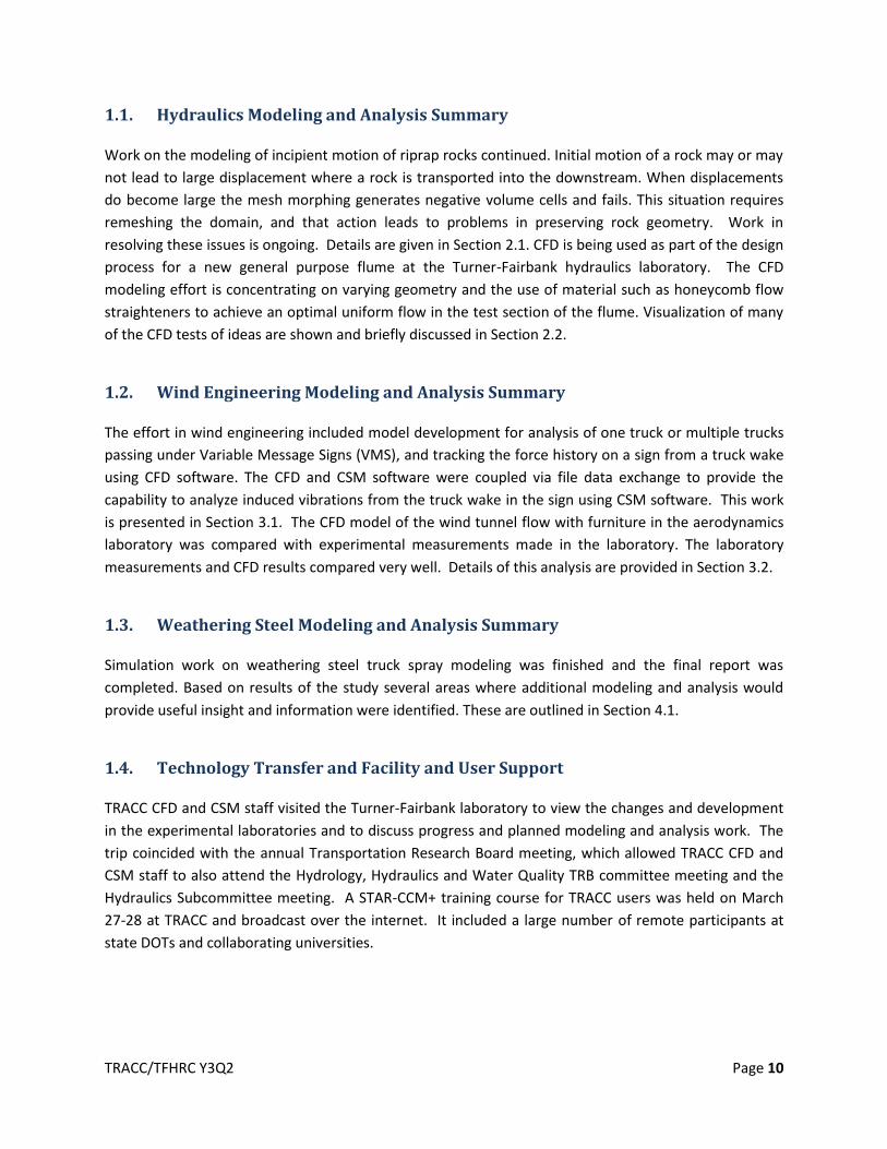
1.1. Hydraulics Modeling and Analysis Summary

Work on the modeling of incipient motion of riprap rocks continued. Initial motion of a rock may or may

not lead to large displacement where a rock is transported into the downstream. When displacements

do become large the mesh morphing generates negative volume cells and fails. This situation requires

remeshing the domain, and that action leads to problems in preserving rock geometry. Work in

resolving these issues is ongoing. Details are given in Section 2.1. CFD is being used as part of the design

process for a new general purpose flume at the Turner-Fairbank hydraulics laboratory. The CFD

modeling effort is concentrating on varying geometry and the use of material such as honeycomb flow

straighteners to achieve an optimal uniform flow in the test section of the flume. Visualization of many

of the CFD tests of ideas are shown and briefly discussed in Section 2.2.

1.2. Wind Engineering Modeling and Analysis Summary

The effort in wind engineering included model development for analysis of one truck or multiple trucks

passing under Variable Message Signs (VMS), and tracking the force history on a sign from a truck wake

using CFD software. The CFD and CSM software were coupled via file data exchange to provide the

capability to analyze induced vibrations from the truck wake in the sign using CSM software. This work

is presented in Section 3.1. The CFD model of the wind tunnel flow with furniture in the aerodynamics

laboratory was compared with experimental measurements made in the laboratory. The laboratory

measurements and CFD results compared very well. Details of this analysis are provided in Section 3.2.

1.3. Weathering Steel Modeling and Analysis Summary

Simulation work on weathering steel truck spray modeling was finished and the final report was

completed. Based on results of the study several areas where additional modeling and analysis would

provide useful insight and information were identified. These are outlined in Section 4.1.

1.4. Technology Transfer and Facility and User Support

TRACC CFD and CSM staff visited the Turner-Fairbank laboratory to view the changes and development

in the experimental laboratories and to discuss progress and planned modeling and analysis work. The

trip coincided with the annual Transportation Research Board meeting, which allowed TRACC CFD and

CSM staff to also attend the Hydrology, Hydraulics and Water Quality TRB committee meeting and the

Hydraulics Subcommittee meeting. A STAR-CCM+ training course for TRACC users was held on March

27-28 at TRACC and broadcast over the internet. It included a large number of remote participants at

state DOTs and collaborating universities.


2. Hydraulics Modeling and Analysis

2.1. Onset of Rip-Rap Motion using STAR-CCM+ Coupled with LS-DYNA

Work on modeling the onset of rip-rap motion continued with enhancing the coupling between CFD software STAR-CCM+ and CSM software LS-DYNA. All the scripts developed previously for coupling were updated to handle problems encountered in the riprap motion problem. In the coupling, STAR-CCM+ (CFD) computes the pressure distribution on the surface of the stones, while LS-DYNA (CSM) computes the displacements and contact forces of the stones. An explicit coupling scheme is implemented i.e. to compute pressure on the stones, the position of the stones in the previous time step is used. The coupling is on the time step level, and not the inner iteration level. For many engineering problems this form of coupling is good enough provided that the time step between data exchange is sufficiently small. The coupling can be subdivided into following steps:

1. Import displacements from LS-DYNA (zero for the first step) to STAR-CCM+ 2. Morph the mesh in STAR-CCM+ based on the new location of the stones 3. Run STAR-CCM+ for one time step 4. Export new pressure distribution on the stone surfaces in LS-DYNA format 5. Run LS-DYNA to get new displacements caused by the new pressures and calculate interaction

between the stones if needed 6. Export displacements from LS-DYNA to STAR-CCM+ 7. Loop until end criteria are met

The initial analysis concerned geometry presented in Figure 2.1 where only the top rock was free to move. The three others were fixed in place in the CSM simulation. The coupling procedure worked very well in the first several steps - the volume mesh in STAR-CCM+ was morphed each time a new position of the moving stone was imported. The problems occurred when the morphing distance was too big and negative volume cells were created near the surface of the displaced stone. To overcome this obstacle the java macro executing the data import and export had to be modified. An additional step of remeshing the domain was implemented. That step allowed for further motion of the stone and coupling between the solvers. Initially undetectably, after several remeshing cycles the shape of the moving stone started to degenerate. The new surface mesh that is the basis for the next time step volume mesh was constructed through extraction of the surface from the volume mesh and then remeshing from the new surface mesh. The interpolation and discretion error in surface mesh extraction appears to be constrained to bias the error in a way that does not allow the volume of the fluid domain to shrink near local surfaces. As a consequence, the moving stone shrinks in size through repeated remeshing operations. Figure 2.1 shows stages of the stone motion due to the water flow over it. The shape degeneration starts to be noticeable already in the middle row of the snapshots. A closer look at the final degenerated shape due to multiple volume meshing is shown in Figure 2.2. It was concluded that the only workaround to this problem is to preserve the stones irregular shape by wrapping the stone mesh with a large number of curves called feature curves. The meshing algorithms treat features differently from general vertices defining the position of a surface. For feature curves, the meshing algorithm tries to maintain the geometry of the curve within a much smaller tolerance than that of the surface in general. Feature curves are used primarily in initial mesh generation to maintain sharp edges and corners. The implementation of this process has begun and will be presented in the following quarterly report.


Figure 2.1 Stages in the coupled simulation for water induced stone motion

Figure 2.2 Problem with multiple remeshing without preserving geometrical features


2.2. Flume Design Modeling at TFHRC

The Hydraulics Laboratory of TFHRC is in the process of designing and building a new hydraulic testing

flume. It is targeted at satisfying physical experiment demand in the coming decades. One of the crucial

parts in designing the flume is the flow inlet assembly. It conditions the flow coming from the pump and

produces proper flow conditions for testing. The performance of the inlet assembly must be able to

yield a uniform flow within a reasonable tolerance across the test section under a variety of different

Froude numbers. The performance is measured by the flow profiles at the inlet to the test section. A

number of simulations were done to identify the best design approach and parameters that offer

optimal performance.

Upon detailed discussions and consultation with venders, it was determined that the pipeline should

enter the inlet assembly from below. This design offers simplicity and minimizes pipeline loss. A trumpet

is located between the pipeline connection and the test section to produce a smooth contraction both

vertically and horizontally. The transition curve formulas and proper range of parameters are obtained

from a parametric study by Hunter Rouse and M. M. Hassman. Variations were made to the parameters

within the given range and to other design features, such as the pipe inlet diffuser and

filters/honeycombs, to see their effects and to find the optimal combination for a multipurpose flume.

The results from these variations are illustrated below:

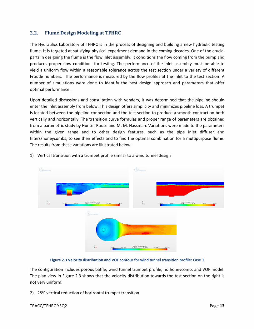
1) Vertical transition with a trumpet profile similar to a wind tunnel design

Figure 2.3 Velocity distribution and VOF contour for wind tunnel transition profile: Case 1

The configuration includes porous baffle, wind tunnel trumpet profile, no honeycomb, and VOF model.

The plan view in Figure 2.3 shows that the velocity distribution towards the test section on the right is

not very uniform.

2) 25% vertical reduction of horizontal trumpet transition


The vertical distance of horizontal transition is reduced by 25% of the original dimension in order to

avoid the separation zone and velocity gradient (Figure 2.4). Three sub-cases were simulated: (a)

Without honeycomb, (b) With honeycomb, and (c) with the diffuser positioned closer to left end of the

flume with honeycomb.

Figure 2.4 Dimensions sketch for 25% reduction of vertical transition

a. Without honeycomb

Figure 2.5 Velocity magnitude contour without honey comb: case 2a

b. With honeycomb

Figure 2.6 Velocity magnitude contour with honey comb: case 2b

c. Closer position of diffuser to left end of flume with honeycomb


Figure 2.7 Velocity magnitude contour with the changed position of pipe diffuser: case 2c

3) 50% vertical reduction of horizontal trumpet transition

a. Without honeycomb

Figure 2.8 Velocity magnitude contour without honeycomb: case 3a

b. With honeycomb

Figure 2.9 Velocity magnitude contour with honeycomb: case 3b

c. Closer position of diffuser to left end of flume with honeycomb

Figure 2.10 Velocity magnitude contour with the changed position of pipe diffuser: case 3c


4) 25% vertical reduction of horizontal trumpet transition with changing from wind tunnel profile to

cubic polynomial curve

a. With the same position of pipe diffuser as case 2a or 2b

Figure 2.11 Velocity magnitude contour and velocity vector: case 4a

b. With longer honeycomb and the same position of diffuser as case 2-c


Figure 2.12 Velocity magnitude contour, velocity vector and free water surface: case 4b

5) Shorter diffuser (other configuration kept the same as case 4a)

Figure 2.13 Velocity magnitude contour and velocity vector for shorter diffuser: case 4

6) New concept diffuser

The new concept diffuser case has a spiral wall profile in the left end and more complicated pipe diffuser

profile.

a. With spiral left-end-wall profile (without honeycomb)


Figure 2.14 Velocity magnitude contour and velocity vector for spiral wall profile: Case 6a

b. With spiral left-wall profile (with honeycomb)

Figure 2.15 Velocity magnitude contour and velocity vector for spiral wall profile: case 6b

7) Porous media cage diffuser with 8 cm of thickness (with wider honeycomb and closer position of

diffuser)


Figure 2.16 Velocity magnitude contour and velocity vector for porous media cage diffuser: case 7

The methodology for analyzing uniformity of flow in flume is significant to select the correct design.

Figure 2.17 Domain for data selection in space

Based on the observations of the numerical simulations, an adequately stable and horizontal free

surface occurs at the box region beginning at a location 1.5 m from the end of the transitional trumpet

and ending at a location 0.5m from the outlet as shown in Figure 2.17. Future plans are to analyze 10-15

vertical sections along the x axis in the box region for each case simulated, and select one position as the

standard so that statistical measures of flow uniformity for different cases can be compared at the same

standard position. The unsteady analysis will be done for a time period of 10 to 20 s at 1 s intervals.

I. Selection of analysis methods

a. Standard deviation

Standard deviation shows how much variation there is for a variable from the average values, which is a

simple and effective method to analyze the uniformity of flow. For our case, the standard deviation is

calculated over the area of a cross section of the channel (surface area in STARCCM+):


√∑ ( )

∑

2.4.1

where is the surface average of physical parameter (velocity magnitude in this case). is the

area.

b. Surface uniformity index (STARCCM+)

The other method uses the surface uniformity index based on the following formula,

∑ | |

∑

2.4.2

which describes the distribution of a certain quantity on one surface. If the physical parameter on one

surface is distributed uniformly, the value of is 1. The design that gives the surface uniformity index

closest to unity is considered having the best performance using this criterion.

The statistical analysis for the flow uniformity based on the finished simulation will be presented in a

future report.


3. Wind Engineering Modeling and Analysis

3.1. Analysis of Sign Vibration Due to Passing Trucks

3.1.1. Literature Review

In this quarter work on analysis of vibration of cantilevered Variable Message Signs (VMS) built over

highways was continued with the main focus on finding a representative loading pattern on the sign box

caused by a passing truck. The research on this subject may be dated back to the late 1970’s, although

the focus was on regular cantilever signs and not VMS, which were not in use at that time. Nonetheless,

for the purpose of finding the pressure on the surfaces of any of these signs they can be treated the

same way. Although a lot more work has been performed in the area of highway sign vibration here we

focus only on the part of it that pertains to the analysis of pressure due to passing trucks.

The first thorough report on this subject was published by Creamer et al. in 1979 [1]. It pertained to

experimental testing of three cantilevered structures instrumented with strain gauges on the sign

supporting truss. Response of the signs to excitation of the sign vibration in horizontal and vertical

directions was analyzed to estimate natural frequencies of the signs and damping ratio (which varied

between 0.49 to 0.70 % of critical damping for vertical motion and from 0.57 to 0.77 % of critical

damping for horizontal motion). The pressure acting on the sign surfaces and the light fixtures wasn’t

analyzed directly. It was back calculated from the measured strains with the assumption of a triangular

impulse function with duration of 0.375 s and a peak of 1.23 psf (58.89 Pa) at 0.125 sec, as shown in

Figure 3.1. A linear decrease of pressure with the height was assumed. The values for the impulse

function were adjusted until calculated member forces matched the forces obtained based on strains

measured in the field tests.

Figure 3.1 Shape of the impulse function assumed by Creamer et. al [1].

Another study was conducted by professors of North Carolina State University in Raleigh and concerned

vibrations of four cantilevered highway sign structures [2]. The work consisted of field testing as well as

wind tunnel modeling. In the field whole signs were investigated. In the wind tunnel testing, the

investigation focused primarily on the trusses without the sign plate. The truss showed high

susceptibility to the vortex shedding induced vibrations. When an attempt was made to attach the sign


plate, the wind tunnel couldn’t develop high enough wind speed to induce similar vibrations. Finite

element analysis was also conducted aiming to study the vibrations of the sign caused by vortex

shedding induced loading indicating that the stresses in the structure were negligible. Buffeting wind

response was also tested with a fluctuating component of the wind velocity formed by a sine function

with frequencies in range from 0.35 to 9.1 Hz, covering several of the first natural frequencies. The

report suggested that this load may cause large stresses in the structure.

One of the cantilevered highway sign structures in the field was instrumented with hot film anemometer

patches to investigate truck-induced gust loading. The researchers determined that the maximum

pressure recorded on the sign due to truck-induced gusts was 1.41 psf (67.5 Pa). It was concluded that

both box-type medium duty trucks and large semi/tractor-trailer trucks produced a similar response on

the cantilevered highway sign structure. The report concluded from both the experimental testing and

analytical modeling that the vibrations of the cantilevered highway sign structure due to truck-induced

gusts did not result in stress levels that would damage the structure. The experimental testing

determined also aerodynamic damping in the horizontal mode of vibration to be 1.17 % of critical and in

vertical mode to be 0.58 % of critical damping.

The study by Cook et al. [3] initiated by Florida DOT describes the most extensive experiments to date,

determining the magnitude, direction, and frequency of truck-induced gust pressure distributions on

VMS. In that work pressure transducers and pitot tubes were instrumented on an existing bridge over an

interstate highway. The testing apparatus could be moved up and down so the gradients of the pressure

acting on the sign were measured. The researchers collected readings from 23 random trucks with the

apparatus at an elevation of 17 ft (5.2 m) above the road surface. To determine the vertical profile of

the pressure variation, three readings were recorded at 17, 18, 19, and 20 ft (5.2, 5.5, 5.8, and 6.1 m)

using a rented control truck moving at a constant speed of 65 mph (29 m/s) for each test. As a truck

passed under the sign, it produced a positive pressure pulse followed by a negative pressure as the end

of the truck passed. The maximum positive and negative pressure magnitudes were in the range of 1 to

2 psf (47.9-95.8 Pa), with a mean pressure magnitude of one psf (47.9 Pa). It was found that for every

foot increase in elevation from 17 ft (5.2 m) above the road surface, the design pressure pulse could be

decreased by 10%. Finally, the significant frequencies of truck-induced gust pressure pulses were

observed to range from 0.5 to 2 Hz. These frequencies are close to the natural frequencies of VMS

structures and could lead to resonance of such structures.


Figure 3.2 Typical truck induced gust pressure history by Cook et al. 1996 [3]

In another study by the same authors [4], design pressures were proposed based on the previously

reported tests.

Table 3.1 Design pressure values proposed by Cook et al. [4]

bottom horizontal surface leading vertical surface

positive pressure (psf) 0.92 1.43

negative pressure (psf) -1.50 -2.10

A group of researchers in [5] presented a simple model for the truck-gust load that incorrectly assumed

the velocity of wind gusts in the upward direction is equal to the truck velocity causing quite substantial

loading on the sign for trucks with over cab air deflectors. The assumption was made based on

misunderstanding of the purpose of the deflectors mounted on modern truck cabins not to deflect the

air 90 deg upward but to make the truck more streamlined and therefore reduce the upward

component of velocity in the wake forming over the cab and top of the trailer to reduce drag. The

researchers used ANSYS software to reconstruct the failure conditions on the VMS structure in Virginia.

The observed amplitude of vibrations of that sign in the field was about 1 ft, and assuming this

deflection, the force causing it was back calculated. This force with an assumed gust factor matched the

force that would be exerted by “deflected” 65 mph upward flowing air from a truck moving at 65 mph.

On that basis they concluded that the theory of deflected air from trucks causing observed sign

vibrations was correct. Although the value of pressure calculated by the formulas proposed by Desantis

and Haig (18.28 psf - 875 Pa, doubled for complete loading cycle) may be good for design purposes as

very conservative, its underlying justification is wrong. These values are significantly higher than the

pressures found in the numerous field studies and the current CFD analysis.


Figure 3.3 Air flow past truck moving 60 mph and assumed air diversion by Desantis [5]

In [6] field tests were performed which resulted in stress ranges below that which would cause fatigue

damage. The researchers concluded that the method proposed by Creamer does not produce accurate

results. In the next model, it was assumed that the velocity of the upward gust is equal to the velocity of

the truck following Desantis incorrect assumption. The authors added a gust factor of 1.3 to the formula

and then doubled the obtained pressure to represent the fact that during one cycle the cantilevered arm

will move both downward and upward. They found a value of 1760 Pa (36.6 psf) to be appropriate to

use as an equivalent vertical static pressure. Subsequently, the Desantis model was recommended in

NCHRP-412 (1998) and then in AASHTO 2001 specifications. It is unfortunate that NCHRP-412 repeats

incorrect assumptions regarding the purpose and effects of air deflectors over truck cabs: “It has been

suggested that the wind deflectors, which are now commonly placed on the cab of tractor-trailers to

improve fuel economy, act as a wedge and produce vertical wind gust pressures larger than those

estimated in previous research”. The proposed values are used as a basis for design procedures. This

comes from misunderstanding of the simple idea using airfoils to increase the fuel efficiency of trucks by

reducing drag. In order to do this the size of the wake must be minimized, and this is done by using the

air deflectors to keep streamlines as close to the truck as possible. NCHRP - 469 reduces reliance on the

high upward deflected flow velocity assumption. It stated that fewer problems have been reported with

VMS over the years between the releases of the two documents, although these structures were not

designed using NCHRP-412 procedures. It also noted that the original design pressure value was based

on limited data. Another series of field tests were analyzed and confirmed that the truck induced gusts

were significantly smaller than the ones assumed in previous report NCHRP-412. In addition, it was

pointed that wrong drag coefficient was assumed for the sign, which should be 1.7. As a consequence,

the magnitude of the design equivalent static pressure equation was reduced to 900xCd Pa (or 18.8xCd

psf), where Cd is the drag coefficient of the sign.

3.1.2. Results of CFD Analysis

In the current quarter CFD analyzes were continued to determine pressure histories acting on the sign

structure due to a passing truck. The models described previously were using unsteady implicit RANS

simulations with a time step of 0.025 sec. The sliding mesh technique was used to move the truck

subdomain through the air domain. In this technique common interfaces are rebuilt at each time step

and the fluid can pass through them. The model consisted of approximately 3,800,000 cells. The CFD

model is shown in Figure 3.4. The number of cases simulated was significantly expanded. Table 3.2

shows all of them. Most of the runs were performed for the truck moving with a velocity of 70 mph

(31.3 m/s) and nominal clearance between the sign bottom panel and the road of 18 ft (5.49 m),


although the height was variable too. Two types of truck cabins were considered as mentioned in the

previous report. The shapes of the cabins used are shown in Figure 3.5. Initially the location of the lanes

under the sign was unknown, so the trucks were located exactly under the center of the sign box. Once

the data on sign position with respect to the road became available the trucks were positioned within

the lane locations. One and two trucks moving side by side were considered.

Figure 3.4 CFD model geometry with interfaces used in sliding mesh motion

Figure 3.5 Trucks without and with over cab flow diverter or non-streamlined and streamlined

Table 3.2 Analyzed cases in the CFD analysis

Truck Velocity Sign height above

the ground Truck shape Wind action Truck location

40 mph 19 ft streamlined,

non-streamlined - center





70 mph 18 ft, 19 ft, 20 ft streamlined, 10 mph center

Global domain

Sliding truck domain

Interfaces between domains


non-streamlined head wind

70 mph 19 ft non-streamlined - left lane, center,

two trucks under the sign

To compare between the cases the pressures acting on the sign with readings from two points were

analyzed (histories are available for the whole sign surface):

– In the middle of front panel near its bottom (element 3145)

– In the middle of the bottom panel (element 2250)

A typical pressure curve on the front panel found in the previous analyses is shown in Figure 3.6. The

curves start with a positive phase when the truck approaches the sign. A negative phase with two local

peaks follows it once the trailer reaches the sign position and the space between the sign box and the

truck is smaller. Another small positive phase ends the pressure history when the truck is past the sign.

The shape of the curve resembles the curves obtained in the experimental studies presented in the

previous section. Its shape will differ depending on the truck and sign shape, truck velocity, wind speed

and other minor effects.

Figure 3.6 Positions of the truck corresponding to the peaks in the pressure history

Close up views of the pressure distribution on the sign surface at the moments of local negative peaks

are presented in Figure 3.7. Only a small patch on the sign panels is loaded with pressure close to the


maximum pressure values. The average pressure on the panels is significantly lower. When the

maximum negative pressure is near 150 Pa, the average pressure can be as low as 40 Pa.

Figure 3.7 Pressure distribution on the sign surface at the time when local negative peaks occur

As the first varying parameter the truck velocity was assumed. The velocity varied from 40 to 70 mph

(17.9 to 31.3 m/s). Figure 3.8 and Figure 3.9 show the pressure histories on the front panel for the

streamlined and non-streamlined trucks respectively. The length of the pressure impulse increases as

the truck speed decreases. The maximum value of negative pressure 59.7 Pa dropped by 67 % to 19.6 Pa

on the frontal panel as the speed drops from 70 to 40 mph for the streamlined truck, and it drops from

69.5 Pa to 22.3 Pa on the bottom panel. In the case of the non-streamlined truck the peak values were

significantly higher. The maximum pressure on the front panel was 94.7 Pa – 59 % more than for the

case of streamlined truck. This value dropped to 34.2 Pa (64 %) when the velocity of the truck was

decreased to 40 mph. The maximum pressure on the bottom panel dropped from 114.6 Pa for the truck

traveling with velocity of 70 mph to 39.7 Pa for the truck with speed of 40 mph.


Figure 3.8 Pressure history on the front panel of the sign for simulations with streamlined truck and different velocities

Figure 3.9 Pressure history on the front panel of the sign for simulations with non-streamlined truck and different velocities

Figure 3.10 Pressure history on the bottom panel of the sign for simulations with streamlined truck and different velocities


Figure 3.11 Pressure history on the bottom panel of the sign for simulations with non-streamlined truck and different velocities

Figure 3.12 shows trends of the maximum negative pressure for the cases summarized here. It can be

concluded that the pressure increases almost linearly for the smooth truck as its velocity increases.

There is slight non-linearity in the pressure increase for the non-streamlined truck. Also the slope of the

fitted linear trend is higher for the non-streamlined truck.

Figure 3.12 Dependency of the pressure on the truck speed

The influence of sign height variation on the pressure magnitude was studied for the non-streamlined

truck traveling with the speed of 70 mph. The same study for the streamlined truck is planned for the

next quarter. Figure 3.13 and Figure 3.14 show pressure histories on the front and the bottom panel in

these cases.

y = 1.33x - 34.38

y = 1.57x - 40.94

y = 1.99x - 46.42

y = 2.44x - 59.54

0

20

40

60

80

100

120

30 40 50 60 70 80

Max

neg

ativ

e p

ress

ure

(P

a)

Truck Speed (MPH)

smooth-front

smooth - bottom

non-streamlined - front

non-streamlined - bottom


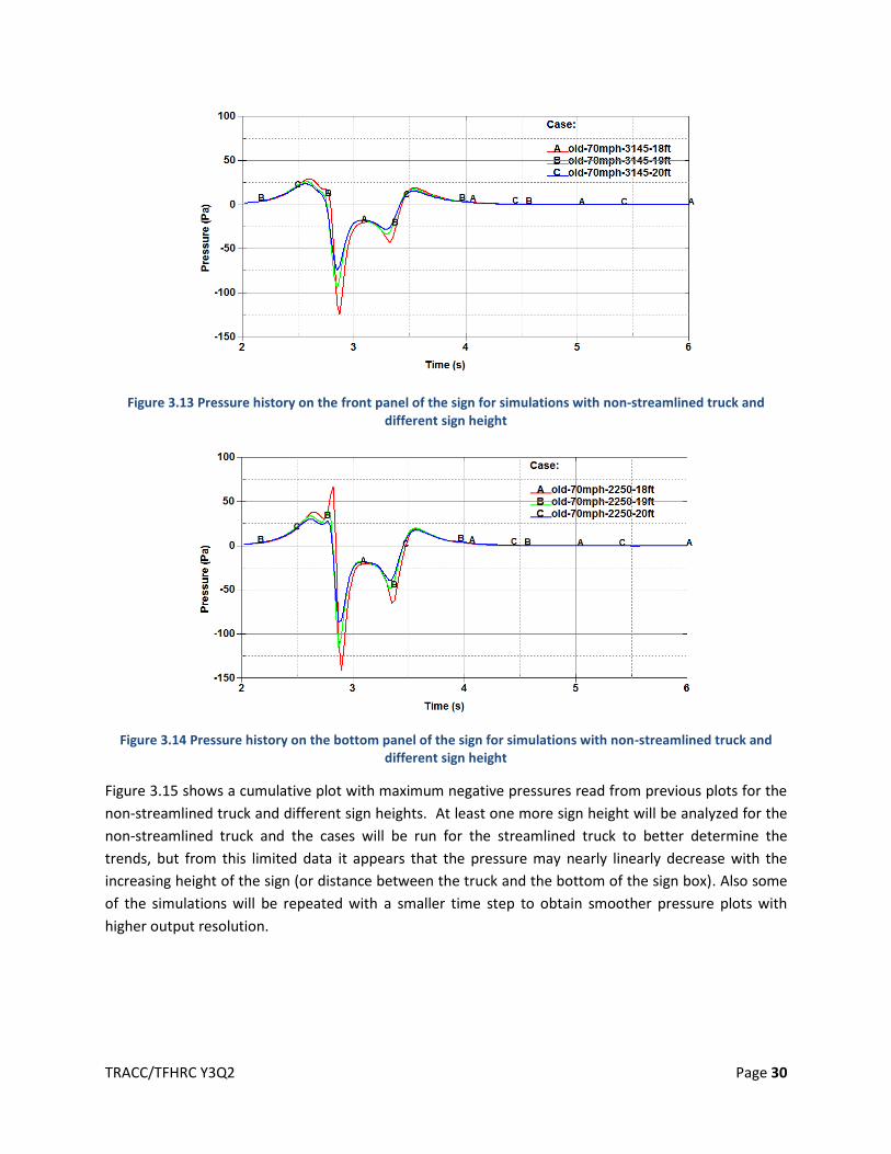
Figure 3.13 Pressure history on the front panel of the sign for simulations with non-streamlined truck and different sign height

Figure 3.14 Pressure history on the bottom panel of the sign for simulations with non-streamlined truck and different sign height

Figure 3.15 shows a cumulative plot with maximum negative pressures read from previous plots for the

non-streamlined truck and different sign heights. At least one more sign height will be analyzed for the

non-streamlined truck and the cases will be run for the streamlined truck to better determine the

trends, but from this limited data it appears that the pressure may nearly linearly decrease with the

increasing height of the sign (or distance between the truck and the bottom of the sign box). Also some

of the simulations will be repeated with a smaller time step to obtain smoother pressure plots with

higher output resolution.


Figure 3.15 Dependency of the pressure on the sign height

Initial simulations were performed with the truck located under the center of the sign - the design

configuration over the road was unknown. Later on, when the drawings were made available, cases with

the truck placed on the left travel lane and two trucks located side by side on two lanes were analyzed.

Figure 3.16 shows the drawings of sign and its location relative to the travel lanes. Figure 3.17 shows the

model from the case with two trucks side by side.

Figure 3.16 Geometry of the TFHRC sign and its location over the highway lanes

y = -24.821x + 569.46

y = -27.748x + 641.31

50

75

100

125

150

17 18 19 20 21 22

Max

neg

ativ

e p

ress

ure

(P

a)

Sign Height (ft)

non-streamlined - front

non-streamlined - bottom


Figure 3.17 Worst case scenario analyzed - two trucks passing simultaneously under the sign

Figure 3.18 and Figure 3.19 show pressure history on the front and bottom panel respectively for the

cases with the truck moved to the left lane and also two trucks moving side by side. These curves are

compared to the previously obtained pressure history for the case with truck traveling underneath the

center of the VMS box. Looking at the front panel, the maximum pressure in the middle of it dropped to

62.9 Pa. That doesn’t mean the maximum pressure reading has dropped – it has just moved to the side

and the value at the element 3145 has dropped. For the case with two trucks passing next to each other

this value has increased to 144.2 Pa. On the bottom panel the difference between the maximum value

of pressure for one truck passing under the center of the sign and two trucks side by side wasn’t that

big. It has increased from 114.6 Pa to 128.7 Pa.

Figure 3.18 Comparison of the pressure histories on the frontal panel due to different truck configuration under the sign


Figure 3.19 Comparison of the pressure histories on the bottom panel due to different truck configuration under the sign

Figure 3.20 and Figure 3.21 show pressure histories for the case with two trucks traveling side by side

and an additional constant head wind with speed of 10 mph (4.47 m/s). The wind has visibly contributed

to the maximum values of the pressure on the front and bottom panels. The maximum pressure at the

measuring point on front panel (element 3145) grew to 183.0 Pa (from 144.2 Pa) and to 165.3 Pa (from

128.7 Pa) on the bottom panel. The pressure change on the back of the sign was not monitored here but

the wind mostly influenced that side of the sign. The following structural analysis was taking into

account the pressure distribution on the whole sign box surface.

Figure 3.20 Pressure history on the sign frontal panel due to 10 mph head wind and passage of a two trucks under the sign


Figure 3.21 Pressure history on the sign bottom panel due to 10 mph head wind and passage of a two trucks under the sign

3.1.3. Results of Structural Analysis

The pressure history on the sign found in CFD analysis was subsequently used in structural analysis of

the sign. Initially a one way coupling between STAR-CCM+ and LS-DYNA was implemented, meaning the

structural analysis in LS-DYNA was performed after the CFD analysis with no iteration back and forth

between CFD and CSM software. In order to obtain pressure histories for all the finite elements in the

sign structure from pressure maps found in CFD, Python scripting was used. That produced 7,500

pressure histories out of 125 pressure maps – 3.125 sec of relevant data.

As a first set of simulations an eigenvalue analysis was performed on the simplified sign structure. The

LS-DYNA finite element model was built based on shell elements. At the time the model was built, the

exact weight of the sign box was not known. All the structural elements of the cantilever structure

supporting the sign were well described. Experimental values of first two natural frequencies were

obtained in the field through a fast Fourier transform (FFT) of the vibration history of the sign in forced

pull-down and push-forward tests. The first natural frequency for the twisting mode was estimated to

be 0.87. For the hatchet mode of natural frequency (the second mode) the eigenvalue was estimated to

be 1.22.

Figure 3.22 shows the first 8 eigenmodes obtained using the LS-DYNA eigensolver. The values for them

were as follows: (1) 0.9169, (2) 1.396, (3) 2.126, (4) 2.557, (5) 3.427, (6) 3.978, (7) 4.579, and (8) 4.959.

Considering the fact that the sign box wasn’t precisely modeled – its stiffness due to unknown internal

structure was unknown. Also its mass was not confirmed until later, and the information about the

catwalk was not available. Even without this information, the first two eigenvalues were close to the

experimental values. The model was further used for vibration analysis due to the load exerted by the

passing trucks.


Figure 3.22 Eigenvalues and eigenmodes for the TFHRC sign model

The implicit solver with a time step of 0.005 s was used to analyze the vibrations of the sign due to

different loads. The model consisted of approximately 20,000 finite elements modeled with elastic

material. As mentioned before, the loading pulses from CFD lasted no longer than 3 s. However, for

most of the runs 60 seconds of real time were simulated.

Similar to the real experiment, push-forward and pull-down tests were simulated to find out which

vibration modes are most excited in such cases. Figure 3.22 shows X and Z components of cantilever tip

vibration history due to gravity and push forward force (X direction) applied for a short time. Figure 3.23

shows Fourier transform of these curves. An obvious peak can be noted from the transform of the X

component corresponding to the first vibration mode (frequency 0.912 Hz). Two peaks can be noted for

frequency 1.40 Hz (second mode) and 2.57 Hz (fourth mode) for the Z component.


Figure 3.23 Free vibration history of the cantilever tip (left) in the X direction and (right) in the Z direction due to gravity and forward force impulse (X direction)

Figure 3.24 FFT of the free vibration history of the cantilever tip (left) in the X direction (right) the Z direction due to gravity and forward force impulse (X direction)

For the pull down impulse test a similar analysis was performed. X and Z displacement histories were

plotted (see Figure 3.25) and their FFT was obtained (see Figure 3.26). This time on both FFTs the second

natural frequency 1.40 Hz is noticeable as well as the 2.22 Hz for the X FFT which may correspond to the

third natural frequency. Thus the first four modes of vibration can be expected from a loading pattern

similar to the push-forward and pull-down tests.


Figure 3.25 Free vibration history of the cantilever tip (left) in the Z direction and (right) in the X direction due to

gravity and pull down impulse (X direction)

Figure 3.26 FFT of the free vibration history of the cantilever tip (left) in the Z direction and (right) in the X

direction due to gravity and pull down force impulse (X direction)

A similar analysis has been performed for the loading coming from passage of a single truck. The

vibration history for this loading is shown in Figure 3.27. FFTs of these curves are shown in Figure 3.28.

Figure 3.27 Free vibration history of the cantilever tip (left) in the Z direction (right) in the X direction due to truck passage


Note that the first, second, third, and probably sixth mode of vibration are excited by this load.

However, all the vibration modes associated with local vibration of the sign faces may be spurious and

only come from the fact that the inner structure of the sign box was not modeled and they are a

consequence of assumed stiffness of the box. Nonetheless, the most apparent first two modes pertain

to the global vibration of the sign.

Figure 3.28 FFT of the free vibration history in the Z direction of the cantilever tip due to truck passage

After the initial analyzes it was already clear that isolated loading from passage of one truck cannot

cause any excessive vibration on the sign. Figure 3.29 presents the vibration history in the Z-direction

from passage of one truck. During the first 2 seconds of simulation gravity loading is applied together

with large damping to remove any vibrations coming from sudden application of loads. After that the

damping is lowered to 1 % of critical damping and the load from the truck is applied. The amplitude of

vibrations was less than 1 inch.

Figure 3.29 Vibration history of the cantilever tip in Z direction caused by passage of one truck

To see what effect multiple trucks passing under the sign can have, the loading curve from passage of

one truck has been used three times with a time offset of 1.4 sec – corresponding to the second natural

frequency. Such spacing of the vehicles would be the worst case scenario. Figure 3.30 shows vibration


history for the sign tip in the Z direction from two simulations with and without structural damping. The

deflection was larger but still was not higher than 1 inch.

Figure 3.30 Vibration history of the cantilever tip in Z direction caused by passage of three trucks

(left) no damping (right) 1% of critical damping

In the field it was observed that passage of a single truck was exciting the sign so the amplitude of

vibrations was around 1 foot. From the simulations conducted so far it was clear that the loading coming

from trucks is not able on its own to force such large vibrations. One more, very unlikely event was

simulated with the loading coming from 20 trucks passing with exactly the same speed maintaining the

worst possible spacing, corresponding to the second natural frequency. The load curves used in this

simulation had a shape similar to the one shown in Figure 3.31

Figure 3.31 Typical pressure history acting on one element of front panel coming from combined load from 20 trucks passing under the sign

Figure 3.32 shows vibration histories for the sign tip in the Z direction. In the case without damping the

amplitude of vibrations was about 2 inches. With the damping it was even smaller. The conclusion

drawn from these simulations is that the truck passage on its own cannot excite the sign to the extent

reported in the field. One hypothesis that will be tested in the following quarters is that the interaction


between the sign and the air has to be modeled in a two way coupling and wind action has to be

modeled. There is a possible interaction between the loads coming from the wind and the trucks that

together may lead to some forms of galloping.

Figure 3.32 Vibration history of the cantilever tip in Z direction caused by passage of twenty trucks (left) simulation without structural damping (right) with 1 % of critical damping

Another, more dramatic case was simulated with trucks passing next to each other on two travel lanes

with a head wind blowing at a speed of 10 mph. The loading curves were built to represent a group of

six trucks, three trucks in two rows. The curve representing vibration of the sign tip in this case is shown

in Figure 3.33. Again, a one way coupling did not allow for full FSI which might have triggered larger

amplitude vibrations.

Figure 3.33 Vibration history of the cantilever tip in Z direction caused by passage of six trucks and 10 mph head wind

3.1.4. Summary

Pressure histories for two truck shapes, four velocities, and three sign heights were analyzed. Different

locations of the truck under the sign were also considered. CFD provided pressure curve estimates that


agree reasonably well with historical experimental data as in terms of the shape and the level of the

pressure variation.

The mass and stiffness of the sign box were not calibrated and that may influence some of the natural

frequencies, however it shouldn’t significantly change the observed trends.

One way coupling between the CFD and CSM software did not indicate any cases leading to excessive

vibrations. The analyzed worst case scenario with 20 consecutive trucks with constant space between

them is unlikely to happen in reality. Thus, the analysis conducted so far indicates that the source of

excessive vibrations in the sign may potentially come from interaction between vibrations induced by

the natural wind gusts and the truck passage.

Currently two way coupling models are being developed to capture the inherent interaction between

the structure vibration and the air flow around it. For these models wind action will be introduced

together with the pressure gusts from the passing trucks.

Additionally CFD analysis will be performed on a stationary rigid sign with wind blowing from different

directions at an increment of 5 degrees to analyze drag and lift force coefficients for the sign.

3.1.5. References

[1] Creamer B.M., Frank K.H., and Klingner R.E., (1979) “Fatigue Loading of Cantilever Sign

Structures from Truck Wind Gusts.” Report No. FHWA/TX-79/10+209-1F, Center for Highway

Research, The University of Texas at Austin

[2] Edwards J.A., and Bingham W.L., (1984) “Deflection Criteria for Wind Induced Vibrations in

Cantilever Highway Sign Structures.” Report No. FHWA/NC/84-001, Center for Transportation

Engineering Studies, North Carolina State University

[3] Cook, R. A., Bloomquist D., Agosta A.M., and Taylor K.F., (1996), “Wind Load Data for Variable

Message Signs.” Report No. FL/DOT/RMC/0728-9488, Engineering and Industrial Experiment

Station, University of Florida

[4] Cook R.A., Bloomquist D., Agosta A.M. (1997)2 “Truck Induced Dynamic Wind Loads on Variable

Message Signs.” Transportation Research Board, Paper No. 970244, 187-193.

[5] DeSantis P.V., Haig P.E, (1996) “Unanticipated Loading Causes Highway Sign Failure”, ANSYS

Convention, 3.99-3.108.

[6] Kaczinski, M.R., Dexter, R.J. and Van Dien, J.P. (1998) “Fatigue Design of Cantilevered Signal,

Sign, and Light Supports.” NCHRP Report 412, Transportation Research Board, Washington, D.C.

[7] Dexter R.J., Ricker M.J., (2002), “Fatigue-Resistant Design of Cantilevered Signal, Sign, and Light

Supports.” NCHRP Report 469, University of Minnesota, Minneapolis, MN


3.2. Wind Tunnel Model Comparison with Laboratory Experiments

A comparison of laboratory air speed measurements with CFD calculated values was done to provide a

means to calibrate the fan exit flow speed model and verify that flow predictions in the test zone at the

outlet of the wind tunnel are adequately accurate. The fan model cage and blade geometry did not

match that of the fan in the laboratory. The fan is old, although functioning very well, and details of the

interior design of the fan blades and geometry are not readily available to construct an accurate,

detailed CAD model of the fan, and the expense of doing it may not be justified. With the fan model

running in a rotating reference frame, assigning a rotational speed equal to that of the laboratory test

was found to under predict velocities at the wind tunnel exit by more than a factor of two. Most of the

discrepancy is likely due to the inaccurate representation of the fan geometry, but some may also be

due to the use of the rotating reference frame without the large computational additional expense of

using a moving mesh. Because the primary zone of interest is at the exit of the wind tunnel, where test

models are placed, an accurate fan geometry model may not be required at all. The interior of the

tunnel, with screens between sections, is designed to produce a uniform flow at the outlet, even if the

flow at the inlet, coming off the fan is significantly non-uniform. The test described in this section

replaces the fan model with a velocity inlet that can be calibrated for a variety of fan rotational speeds.

A uniform inlet velocity was then adjusted to match one measured point for the 118 RPM fan case, and

results were compared to air speeds measured at 2.13 m (7 ft) above the floor.

3.2.1. Replacement of Fan Model with Specified Velocity Inlet and Pressure Outlets

Figure 3.34 shows the zones in the fan section of the wind tunnel, consisting of the fan, a swirl zone

where air comes off of the fan blades and flows toward the entry chamber of the wind tunnel, and the

entry chamber of the wind tunnel. This entire zone was isolated from the model by creating flat

boundaries at the inlets and exit of the fan chamber to separate it from the room and the interior of the

wind tunnel. The flow model is now the interior of the wind tunnel and the surrounding room, with the

fan chamber excluded from the model. The inlet to the flow model in the rectangular inlet to the wind

tunnel inlet chamber is shown in Figure 3.35, highlighted in pink. It is defined as a specified velocity

inlet. The exits of the flow model are flat circular boundaries positioned at the narrowest part of the

contracting fan chamber wall leading from the room into the fan as shown in Figure 3.36 highlighted in

pink for the fan inlet on the far side of the room. These room exit boundaries are defined as pressure

boundaries so that the flow split ratio on the two sides can be solved for as part of the model

computation.


Figure 3.34 Zones in the fan section of the wind tunnel


Figure 3.35 Portion of fan chamber showing inlet to wind tunnel in pink highlight

Figure 3.36 Portion of fan zone showing boundary between room and fan section in pink highlight

3.2.2. Determination of Inlet Velocity for Chamber Section

The volume flow through the rectangular wind tunnel entry shown in Figure 3.35 is not known for a

given fan rotation speed. For this analysis the velocity across this inlet is assumed to be uniform, and it


was iteratively adjusted until the velocity matched the laboratory measurement point 20, shown in

Figure 3.39. This matching procedure is one way to use the CFD computation to calibrate the volume

flow generated by the fan with the rotation speed of the fan. For the case with the motor running at

400 RPM and fan at 118 RPM, the velocity at measurement location 20 was 10.5 m/s (23.5 mph), and

the average tunnel inlet boundary velocity required to match it was 21 m/s (47 mph).

3.2.3. Comparison of Laboratory Measurements and CFD Results

The computed velocity vector field at the laboratory measurement height is shown in Figure 3.37. The

velocity vector field plotted from the laboratory measurements is shown in Figure 3.38. Vector lengths

are proportional to velocity, however, they are scaled differently in the two figures to better show the

flow pattern. The CFD results yield much more detail than the laboratory measurements. Note

however, that the laboratory measurements at 2.1 m elevation included over 60 measurement locations

in the room. As seen in the figures, the qualitative features of the flow field match reasonably well. The

jet leaving the wind tunnel turns slightly to the right, as viewed from the fan end of the room, in both

the CFD results and the measured values. Recirculation zones in the downstream end of the room are

visible in both figures.

For a more quantitative comparison, computed and measured air velocities are compared across the

wind tunnel jet downstream of the wind tunnel exit in Figure 3.40 to Figure 3.42. The CFD analysis

predicts a slight asymmetry in the velocity distribution across the jet, as noted in previous sections. The

measured values compare well to the computed values in the asymmetric distribution after matching of

the velocity magnitude at point 20 via adjustment of the inlet velocity as described in Section 3.2.2.

While the pattern of the distribution is similar, the CFD analysis under predicts the velocity on the right

side of the room in the last row of measurement points near the far wall, Figure 3.42. In this location the

computation is sensitive to the position of the stagnation point on the far wall. The jet at the exit of the

wind tunnel is clearly influenced by the presence and location of the room walls. The confinement of

the end wall forces the jet to stagnate, turn, spread out along the end wall, and ultimately turn back

along the side walls to provide the return flow to the wind tunnel fan. Whether or not the asymmetry in

the jet flow is sufficient to adversely influence drag, lift, moment, etc. measurements on objects placed

in the test section just downstream of the wind tunnel exit is not addressed in the scope of this study.

The presence of this asymmetry has been confirmed with the laboratory measurements.


Figure 3.37 CFD computed velocity vector field at the height of the laboratory measurements

Figure 3.38 Vector field plotted from laboratory measurements


-6-4-202468

1012

-10 -8 -6 -4 -2 0

Y V

elo

city

(m

/s)

Position across room (m)

Velocity profile at Y = 12.4

CFD Y =12.38

Figure 3.40 Comparison of measured and computed velocity distribution at the second set of measured points spanning the room in the downstream of the wind tunnel jet.

-6

-4

-2

0

2

4

6

8

10

12

-10 -8 -6 -4 -2 0

Y V

elo

city

(m

/s)



CFD Y = 10.86

Lab Y = 10.86

Figure 3.39 Comparison of measured and computed velocity distribution at first column of points that spanned the room. Point 20 was matched in the computation by adjusting the wind tunnel mean inlet velocity.


-4

-2

0

2

4

6

8

10

12

-10 -8 -6 -4 -2 0

Y V

elo

city

(m

/s)



CFD Y = 13.91

Lab Y = 13.91

-4

-2

0

2

4

6

8

10

12

-10 -8 -6 -4 -2 0

Y V

elo

city

(m

/s)



CFD Y =15.43

Figure 3.41 Comparison of measured and computed velocity distribution at the third set of measured points spanning the room in the downstream of the wind tunnel jet.

Figure 3.42 Comparison of measured and computed velocity distribution at the fourth set of measured points spanning the room in the downstream of the wind tunnel jet.

While the comparison between velocities computed with the CFD model and laboratory measurements

at 2.1 m elevation in the main portion of the jet at the wind tunnel exit were quite good, the comparison


along the return path to the fan near the walls is not nearly as good. The CFD computation uses a k-

epsilon turbulence model, which is based on averaging the Navier-Stokes equations. However, the flow

field computed in such a model does not necessarily correspond to average velocities over the entire

domain of the room. Because the room in the model is a closed system, all of the air leaving the fan

chamber should eventually re-enter the fan chamber through the two pressure exit boundaries on the

sides of the fan chamber. In the computation, this condition, mass balance, is met very well. An air flow

of 41.88 kg/s is propelled down the tunnel by the fan, and 41.88 kg/s enters the fan chamber from the

room, 22.50 kg/s from the right and 19.38 kg/s from the left fan entry. That is a mass balance of four

significant figures, which is quite good, for this type of computation in a complex geometry with nearly

all of the furniture in the room represented in the model as well as the geometry of the tunnel,

turbulence generator, etc. The eddy viscosity in the k-epsilon model determines the mean transport

rate of momentum due to large fluctuating eddies in the room that are averaged out in the model.

This includes the mixing with air surrounding the jet, which controls the entrainment rate and

consequently, in part, the velocity distribution across the jet. These results compared well with lab

measurements. The various obstructions in the room and the eddy viscosity contribute to determining

the paths of least resistance for air to return to the fan. Since all air (to 4 digits) makes it back to the fan,

over estimation of velocity at 2.1 m height near the right wall as shown in Figure 3.43, must be offset by

under prediction at some other parts of the room. The velocities in Figure 3.43 show the correct trend,

but the over prediction is fairly large between about the 6 m and the 11 m position. This region is not

near the test section of the wind tunnel so error in this part of the domain does not have significant

implications for testing the effects of wind on objects places in the wind tunnel jet.

Figure 3.44 shows a comparison of the measured and CFD computed mean velocity near the wall with

the turbulence generator. The measurement points are shown circled in red. In this case the trend in

velocity along the near wall return path to the fan is different at the measurement height between the

measurements and the CFD calculations. The difference is approximately in the position of the

turbulence generator, which represents a significant bluff body in the flow return path along the far

wall, even though the vanes were open during measurement and in the model. The blockages of the

sides of this object create a recirculation zone in the middle of the generator with a low velocity near

the center of that zone. In reality, the sides of the generator may be shedding vortices that show up in

measurement as significant velocity. The CFD turbulence model cannot capture vortex shedding

accurately and the recirculation zone that results from the turbulence is steady and forces flow going

back to the fan entry to bypass it. This situation appears to be the most likely cause of the measured

and computed differences shown in Figure 3.44.


Figure 3.43 Measured and CFD velocity magnitude near the wall with the door (circled measurement points)

0

0.5

1

1.5

2

2.5

3

3.5

4

-10 -5 0 5 10 15 20

Y V

elo

city

(m

/s)A

Position along door wall (m)

Velocity Near Door Wall x = -1.52

CFD

Lab


Figure 3.44 Measured and CFD velocity magnitude near the wall with the turbulence generator (circled measurement points)

0

0.5

1

1.5

2

2.5

3

3.5

4

4.5

-10 -5 0 5 10 15 20

Ve

loci

ty (

m/s

)

Position along turbulence generator wall (m)

Velocity Near Far Wall x = -8.23

CFD Lab


4. Weathering Steel Truck Spray Modeling and Analysis

In the current quarter the simulation work on weathering steel truck spray modeling was finished and

the final report was completed. Based on results of the study several areas where additional modeling

and analysis would provide useful insight and information were identified. These are outlined in the

following section.

4.1. Topics for Future Analysis

A significant portion of the work in conducting the study involved identifying the droplet size range of

interest, setting up and testing the advanced sliding mesh models for moving a truck or trucks under the

bridge, determining the level of detail in truck geometry that is sufficient to capture the physics of flow

past the truck and yields numerically stable results, testing droplet injection methods, etc. Now that a

functioning model has been built that will converge for a variety of conditions and geometry changes,

follow on studies with the model can be conducted with much less setup work. The following areas are

among many that are good candidates for future study.

1. Effect of clearance between bottom of the girders and the top of the truck in both calm air and

wind conditions

Droplet number histograms under the bridge show a rapidly decaying tail with height above the

road. Therefore, when the bridge girders are higher above the road, smaller numbers of

droplets would be expected to reach the girders. However, because small wind velocities are

easily able to carry droplets in the size range of interest upward, bridge height might be a

significant parameter in the absence of wind but much less significant in the presence of wind.

2. Effects of the width of the bridge (number of lanes)

The bridges studied were 4 lanes wide. The effects on droplet transport when the truck and

flow are confined between bridge and road for a bridge with eight or even twelve lanes have not

been investigated. At least one weathering steel bridge with a large number of lanes is known

to have a problem with accelerated corrosion rates, and therefore bridge width is a parameter

that is worth investigating.

3. Effects of wind velocity with full bridge geometry modeled, in particular average and very low

velocities

Studies of wind effects were limited due to time and funding available in the initial study. To

complete the first set of cases in the time available and identify the relative importance of wind

effects, the same computational domain and mesh was used for the wind cases as was used for


other parameters. This was a half domain that cut through the center of the bridge. The

geometry did appear to be very significant in cases with wind because obstructions change the

wind direction. The full bridge geometry should therefore be included to assess wind effects

when the direction of the wind is at an angle with respect to the road.

4. Injectors of parcels for the cases with the wind located on both sides of the truck

To save computation time and resources nearly all cases ran with the spray coming only from

tires on the curb side of the truck because that side would experience the effects of the

different bridge abutment geometries that were tested. For cases with full bridge geometry on

both sides of the road and wind, droplets should be injected from tires on both sides of the

truck. Means to reduce the number of parcels tracked would be investigated in order to keep

simulation times from becoming unacceptably large.

5. Effects of smaller vehicle traffic such as a car following a truck or a car following a car

When a truck entrains droplets from the roadway into its wake, they tend not to rise much

above mid trailer height in the absence of wind or following vehicle traffic. The initial study

found that a following truck that was the same height as the lead truck could loft suspended

droplets upward to bridge girders as the wake flow of the first truck gets diverted up and over

the following truck. Smaller following vehicles would also divert the wake flow of a lead vehicle

upward. Simulations can be run to see if the upward velocity caused by a less tall following

vehicle, such as a car, is sufficient to carry significant numbers of droplets suspended by the lead

vehicle to the bridge girder level.

6. Effect of a non-aerodynamic truck cab

Most modern trucks have aerodynamic trucks cabs that minimize the size of the separated flow

wake. The larger wakes of trucks that do not have this streamlining can be tested easily to

assess the magnitude of the effects of non-aerodynamic following in the spray laden wake of a

lead truck.

7. Additional study of dry aerosol size particulate erosion from road surface and transport

A very limited number of cases were tested using dry aerosol transported as a component of the

air. Because the salt film remaining on the road days after a snow event can be substantial, and

this film is eroded and suspended in the air by traffic, further investigation of transport of

aerosol in combination with wind may yield additional insight on salt transport mechanisms.

8. Other minor geometry effects such as girder spacing and girder depth

Girder spacing and girder depth determine the geometry and scale of the cavity between

girders. Large trucks passing under the bridge induce a recirculating cavity flow between

girders. Running cases that vary these geometry parameters would help to determine their


impact on deposition rates of salt on girders. Additional physics models that include deposition

would have to be developed and implemented to investigate these effects.

9. Modeling of one or two real bridges that have known issues with accelerated corrosion

A comparison of real bridges that have known issues with accelerated corrosion to one that

does not while keeping droplet entrainment rates, wind speed and direction, etc., the same may

help to identify the causes of accelerated corrosion in the problem bridges.

10. Verification of trends observed in CFD simulation with field measurements

Some field tests have been proposed to do field measurements using LiDAR to obtain the

droplet mist distribution to characterize the density and extent of the droplet plume coming

from a truck. CFD simulation would be done for these tests to assess how well the RANS

turbulence model used in the simulation does in combination with how the Lagrangian droplet

transport model does in predicting the trends in droplet transport from truck wakes.


5. Technology Transfer

TRACC CFD staff visited the Turner-Fairbank laboratory in January during the annual Transportation

Research Board (TRB) meeting week. The meeting included tours of the hydraulics and aerodynamics

laboratories with discussions of current and planned experiments. CFD and CSM modeling progress and

plans for the coming quarters were also discussed during the meeting. TRACC modeling staff was able

to attend the Hydrology, Hydraulics and Water Quality (AFB60) TRB committee meeting and the

Hydraulics Subcommittee meeting AFB60(2) during the trip. Attendance at these committee meetings

help to keep TRACC modeling staff up to date on topics of current interest in these areas.

CFD collaborator video conferences were held every other Thursday morning between TRACC, TFHRC,

and other transportation researchers using the TRACC clusters for CFD analysis. Graduate student

researchers and occasionally their advising professor at the University of Florida joined the sessions to

expand their experimental program by adding CFD analysis of their experimental flume. A bridge

engineer from California DOT working to apply CFD to practical problems in river hydraulics near bridges

for the state was also a regular in the videoconferences.

A training course in applying the CFD software STAR-CCM+ to problems in hydraulics and wind

engineering was held on March 27-28 at TRACC and included a large number of remote participants at

state DOTs and collaborating universities. As many as 18 remote locations were observed following the

training sessions as they were broadcast via Adobe Connect over the internet. Some of the remote

locations were meeting rooms with several people in attendance. Remote participants were able to ask

questions during the sessions via a chat window in the Adobe Connect session. The questions asked and

answered by instructors indicated that the remote participants were following the training closely.

Figure 5.1 shows attendees at the Argonne site in the large videoconferencing and training room during

one of the training sessions. The training now employs a set of tutorials on hydrodynamics and wind

engineering problems developed over the past several years to teach students how to apply the CFD

software to these types of problems. The training sessions included tutorials on the STAR-CCM+ user

interface, modeling free surface flow in a channel, computing the force of a truck generated wake on an

over highway sign using sliding mesh capabilities for the relative motion between the truck and sign,

analyzing the force on a flooded bridge deck, applying the dynamic fluid body interaction model to

analysis of the vibration of a section of bridge stay cable in a wind tunnel, computation of culvert flow

using cyclic boundary conditions, computing fluid flow in a domain with a propeller and a free surface, a

simplified example of clear water pressure flow scour, computation of wind force on adjacent road

signs, and analysis of droplet transport from a truck tire spray.


Figure 5.1 CFD training class session in the large videoconferencing and training room


6. TRACC Facility and User Support for TFHRC

The new Zephyr cluster is now in production mode and TRACC users in the CFD and CSM application

areas are being encouraged to use it. The TRACC Wiki has been updated to include changes needed for

users to run on either of the TRACC clusters. The application notes for STAR-CCM+ and the LS-DYNA

related software have been updated to include information for the new Zephyr cluster.

Energy Systems Division Argonne National Laboratory 9700 South Cass Avenue, Bldg. 362 Argonne, IL 60439-4815 www.anl.gov Argonne National Laboratory is a U.S. Department of Energy laboratory managed by UChicago Argonne, LLC

http://www.anl.gov/

computational mechanics research and support for ... mechanics research and support for aerodynamics...

Documents