computational fluid dynamics-modelling of a multi-stage
TRANSCRIPT

Computational Fluid Dynamics-Modelling of aMulti-Stage Transonic Axial-Flow Compressor
by
Philip Nel
Thesis presented in partial fulfilment of the requirements for thedegree of Master of Engineering (Mechanical) in the Faculty of
Engineering at Stellenbosch University
Supervisor: Prof. S.J. van der Spuy
Co-supervisor: Prof. T.W. von Backström
December 2019

Declaration
By submitting this thesis electronically, I declare that the entirety of the work con-tained therein is my own, original work, that I am the sole author thereof (save tothe extent explicitly otherwise stated), that reproduction and publication thereof byStellenbosch University will not infringe any third party rights and that I have notpreviously in its entirety or in part submitted it for obtaining any qualification.
December 2019Date: . . . . . . . . . . . . . . . . . . . . . . . . . . . . . . .
Copyright © 2019 Stellenbosch UniversityAll rights reserved.
i
Stellenbosch University https://scholar.sun.ac.za

Abstract
Computational Fluid Dynamics-Modelling of a Multi-StageTransonic Axial-Flow Compressor
P. NelDepartment of Mechanical and Mechatronic Engineering,
University of Stellenbosch,Private Bag X1, Matieland 7602, South Africa.
Thesis: MEng (Mech)December 2019
This research originates from commercial interest in the numerical modelling oftransonic axial compressors. The Darmstadt R-1/S-1 and NASA Stage-37 transonicstages are used as validation test cases using commercial (ANSYS® CFX®) andopen-source (MULTALL-open) CFD software. Various turbulence models, includ-ing a transition model, are tested. The structure parameter of the SST − γReθmodel is calibrated to reduce over-predicted shock-induced boundary layer sepa-ration and to predict the correct separation behaviour on the Darmstadt stator. Atthe operating point, the numerical and experimental stage pressure ratio and effi-ciency for NASA Stage-37 differ by 0.8% and 0.3%, respectively (1.8% and 1.5%for the Darmstadt test case). Aspects of a specific multi-stage compressor, suchas the effects of fillets and surface roughness are investigated. It was found thatat certain shaft speeds, fillets restrained hub corner stall. Blade surface roughnesshas a greater effect on overall performance than endwall roughness due to for ex-ample, the outward migration of a thickened suction side boundary layer, whichmixes with the tip leakage flow. The difference between transient and steady-stateresults is investigated. Inaccurate treatment of flow features at the mixing plane of asteady-state model gains significance in the modelling of multi-stage compressors.The mixing plane approximation leads to reduced hub corner stall at some bladerows and reduced entropy production by the tip clearance flow. Lastly, the abilityof the MULTALL-open turbomachinery design suite of programs to be used fortransonic axial compressor performance prediction is investigated. Good estimatescould be obtained. The accuracy with which MULTALL resolves typical flow fea-tures of transonic axial compressors such as the tip clearance flow features, is foundto be promising. It is concluded that MULTALL can be used for transonic axialcompressor performance prediction.
ii
Stellenbosch University https://scholar.sun.ac.za

Uittreksel
Berekeningsvloeimeganika-Modellering van ’n Multi-StadiumTranssoniese Aksiaalvloei Kompressor
(“Computational Fluid Dynamics-Modelling of a Multi-Stage Transonic Axial-FlowCompressor”)
P. NelDepartement Meganiese en Megatroniese Ingenieurswese,
Universiteit van Stellenbosch,Privaatsak X1, Matieland 7602, Suid Afrika.
Tesis: MIng (Meg)Desember 2019
Hierdie navorsing ontstaan uit kommersiële belangstelling in die numeriese mo-delering van transsoniese aksiaalvloei kompressors. Die Darmstadt R-1/S-1 enNASA Stage-37 transsoniese kompressor stadiums word gebruik as toetsgevalle virkommersiële (ANSYS® CFX®) en oopbron (MULTALL-open) berekeningsvloei-meganika sagteware. Verskillende turbulensie modelle word getoets, insluitende ’nturbulensie-oorgangsmodel. Die struktuur parameter van die SST − γReθ turbu-lensie model is gekalibreer om oorgeskatte skok-geïnduseerde grenslaag skeiding teverminder en om die korrekte wegbrekingsgedrag op die Darmstadt stator te voor-spel. By die ontwerpspunt verskil die numeriese en eksperimentele drukverhoudingen benuttingsgraad van die NASA Stage-37 toetsgeval met 0.8% en 0.3%, onder-skeidelik (1.8% en 1.5% vir die Darmstadt toetsgeval). Aspekte van ’n spesifiekemulti-stadium kompressor, soos die effekte van vulradiusse en oppervlakgrofheidword ondersoek. Daar is gevind dat by sekere as-snelhede, vulradiusse die naaf-hoek wegbreking verminder. Die grofheid van die lem se oppervlak het ’n grotereffek op die algehele verrigting as die grofheid van die rand a.g.v. bv.; die uitwaartsemigrasie van ’n verdikte grenslaag aan die laagdruk kant van die lem, wat met dielekvloei van die lempunt meng. Die verskil in resultate tussen tyd afhanklike en be-stendigte modelle word ondersoek. Onakkurate hantering van die vloei kenmerkeby die meng-tussenvlak van die bestendige model, word uitgelig in die modelleringvan multi-stadium kompressors. Die meng-tussenvlak benadering lei tot vermin-derde naafhoek wegbreking by party lemrye en verminderde entropie produksie bydie lekvloei van die lempunt. Laastens word die vermoë van die MULTALL turbo-
iii
Stellenbosch University https://scholar.sun.ac.za

UITTREKSEL iv
masjienerie ontwerpsprogramme vir die gebruik van transoniese aksiaalvloei kom-pressor verrigtingsvoorspelling ondersoek. Goeie skattings kon verkry word. Dieakkuraatheid waarmee MULTALL tipiese vloei eienskappe van transsoniese aksi-aalvloei kompressors soos die lekvloei by die lempunt oplos, is belowend. Daarmeeword afgelei dat MULTALL gebruik kan word vir die voorspelling van die verrig-ting van transsoniese aksiaalvloei kompressors.
Stellenbosch University https://scholar.sun.ac.za

Acknowledgements
The author would like to acknowledge the following contributions:
• For their support, Prof. S.J. van der Spuy and Prof. T.W. von Backström, thesupervisor and co-supervisor of this work.
• NUMECA (Germany) for providing the geometry of the Darmstadt R-1/S-1test case of Technische Universität Darmstadt.
• Dr Hannes Pretorius of DeltaV Aerospace. DeltaV Aerospace sponsors thiswork.
• The HPC1 computing cluster of Stellenbosch University.• The CSIR Rosebank CHPC (Centre for High Performance Computing).
v
Stellenbosch University https://scholar.sun.ac.za

Contents
Declaration i
Abstract ii
Uittreksel iii
Acknowledgements v
Contents vi
List of Figures ix
List of Tables xiii
Nomenclature xiv
1 Introduction 11.1 Background and motivation . . . . . . . . . . . . . . . . . . . . . . 11.2 Thesis objectives . . . . . . . . . . . . . . . . . . . . . . . . . . . 4
2 Literature Study 52.1 Supersonic and transonic compressor background . . . . . . . . . . 52.2 Shock waves and shock-induced separation . . . . . . . . . . . . . 72.3 Real geometry effects in CFD . . . . . . . . . . . . . . . . . . . . . 72.4 Roughness modelling . . . . . . . . . . . . . . . . . . . . . . . . . 92.5 Transition modelling . . . . . . . . . . . . . . . . . . . . . . . . . 102.6 CFD Validation . . . . . . . . . . . . . . . . . . . . . . . . . . . . 132.7 Concluding remarks . . . . . . . . . . . . . . . . . . . . . . . . . . 14
3 Validation Test Cases in ANSYS® 153.1 Numerical modelling setup . . . . . . . . . . . . . . . . . . . . . . 153.2 Technical data . . . . . . . . . . . . . . . . . . . . . . . . . . . . . 173.3 Mesh information . . . . . . . . . . . . . . . . . . . . . . . . . . . 183.4 Effect of transition modelling . . . . . . . . . . . . . . . . . . . . . 213.5 Motivation for using the SST − γReθ model . . . . . . . . . . . . 23
vi
Stellenbosch University https://scholar.sun.ac.za

CONTENTS vii
3.6 Adapting the shear stress limiter . . . . . . . . . . . . . . . . . . . 293.7 Concluding remarks . . . . . . . . . . . . . . . . . . . . . . . . . . 30
4 Main Numerical Investigation 314.1 Test case transient and steady-state comparison . . . . . . . . . . . 314.2 Multi-stage compressor mesh . . . . . . . . . . . . . . . . . . . . . 384.3 Baseline multi-stage compressor map . . . . . . . . . . . . . . . . . 404.4 Multi-stage transient and steady-state comparison . . . . . . . . . . 434.5 Effect of blade and endwall roughness . . . . . . . . . . . . . . . . 444.6 Effect of blade fillets . . . . . . . . . . . . . . . . . . . . . . . . . 50
5 MULTALL 535.1 MULTALL as an analysis tool . . . . . . . . . . . . . . . . . . . . 535.2 MULTALL geometry defintion . . . . . . . . . . . . . . . . . . . . 545.3 Multi-stage compressor geometry . . . . . . . . . . . . . . . . . . . 565.4 MULTALL Modelling setup . . . . . . . . . . . . . . . . . . . . . 575.5 Shroud pressure distribution . . . . . . . . . . . . . . . . . . . . . 645.6 MULTALL multi-stage compressor . . . . . . . . . . . . . . . . . . 665.7 MULTALL in a commercial environment . . . . . . . . . . . . . . 69
6 Conclusion 706.1 Validation test cases in ANSYS® . . . . . . . . . . . . . . . . . . . 706.2 Comparison of transient and steady-state results . . . . . . . . . . . 706.3 Effects of fillets and wall roughness . . . . . . . . . . . . . . . . . 716.4 The use of MULTALL for transonic axial compressor performance
prediction . . . . . . . . . . . . . . . . . . . . . . . . . . . . . . . 71
References 72
Appendices 78
Appendix AValidation test cases 79A.1 NASA Stage-37 mesh information . . . . . . . . . . . . . . . . 79A.2 Modelling parameters . . . . . . . . . . . . . . . . . . . . . . . 81A.3 Darmstadt test case . . . . . . . . . . . . . . . . . . . . . . . . . 82A.4 NASA Stage-37 performance curves . . . . . . . . . . . . . . . 83
Appendix BMain numerical investigation 86B.1 Transient vs. steady-state comparison . . . . . . . . . . . . . . . 86B.2 ANSYS® multi-stage compressor mesh . . . . . . . . . . . . . . 86B.3 Transient and steady-state comparison . . . . . . . . . . . . . . . 88B.4 Effect of blade and endwall roughness . . . . . . . . . . . . . . . 88B.5 Effect of fillets . . . . . . . . . . . . . . . . . . . . . . . . . . . 90
Stellenbosch University https://scholar.sun.ac.za

CONTENTS viii
Appendix CMULTALL 91C.1 Geometry definition . . . . . . . . . . . . . . . . . . . . . . . . 91C.2 Modelling setup . . . . . . . . . . . . . . . . . . . . . . . . . . 93C.3 Multi-stage compressor . . . . . . . . . . . . . . . . . . . . . . 95
Stellenbosch University https://scholar.sun.ac.za

List of Figures
1.1 HeS 3 Centrifugal turbojet engine at the Deutsches Museum in Munich(photographer: Hans-Jochum Becker). . . . . . . . . . . . . . . . . . . 2
1.2 Jumo 004B axial turbojet engine illustration (Junkers Flugzeug- undMotorenwerke, 1944). . . . . . . . . . . . . . . . . . . . . . . . . . . . 2
1.3 EJ200 Turbofan engine with highly loaded transonic compressors (Cour-tesy of Rolls-Royce, plc). . . . . . . . . . . . . . . . . . . . . . . . . . 3
2.1 RGW compressor cascade: (a) SST, (b) experimental, (c) SST − γReθ(ANSYS®, 2011) . . . . . . . . . . . . . . . . . . . . . . . . . . . . . 11
2.2 Experimental oil streak lines by Haideng et al. (2015) on the NACA-65K48 high subsonic compressor cascade at varying angles of attack. . . . 11
2.3 "Oil streak visualization of the suction side a single cascade blade over-laid with positions of PIV measurement areas". Reproduced from WillertKlinner (2014). . . . . . . . . . . . . . . . . . . . . . . . . . . . . . . 12
2.4 Darmstadt stator flow separation. (Bakhtiari et al., 2015) . . . . . . . . 13
3.1 Typical computational domain of a compressor stage. . . . . . . . . . . 153.2 Selected mesh topology for ANSYS® CFX® simulations. . . . . . . . . 183.3 An ANSYS® CFX® mesh obtained with the selected mesh topology
(Darmstadt R-1/S-1). . . . . . . . . . . . . . . . . . . . . . . . . . . . 193.4 Orthogonal detail for geometry with fillets. . . . . . . . . . . . . . . . . 193.5 Downstream movement of stator boundary layer transition with de-
creasing y+ in Darmstadt R-1/S-1 test case. . . . . . . . . . . . . . . . 223.6 Rotor turbulent boundary layer comparison of SST −γReθ result (top)
and SST result (bottom) at half span. . . . . . . . . . . . . . . . . . . 223.7 Darmstadt R-1/S-1 performance curves: isentropic efficiency (top), stage
pressure ratio (bottom). . . . . . . . . . . . . . . . . . . . . . . . . . . 243.8 (a): SST − γReθ, a1 = 0.345 and (b): k − ω near peak efficiency (16
kg/s). (c): SST − γReθ, a1 = 0.345 and (d): k − ω near stall (14.8kg/s). Red indicates regions of negative axial velocity. Numerical (e)and experimental (f) stator shear lines. The interpretation of experimen-tal stator shear lines (g). . . . . . . . . . . . . . . . . . . . . . . . . . . 25
3.9 NASA Stage-37 performance curves: stage isentropic efficiency (top),stage pressure ratio (bottom). . . . . . . . . . . . . . . . . . . . . . . . 26
ix
Stellenbosch University https://scholar.sun.ac.za

LIST OF FIGURES x
3.10 Shock induced boundary layer separation at 20 kg/s on NASA Stage-37 rotor blade suction side. (a): SST , (b): SST − γReθ, a1 = 0.31 +Reattachment Production. (c): SST − γReθ, a1 = 0.31. (d): SST −γReθ, a1 = 0.345. (e): k − ω. (f): k − ε. . . . . . . . . . . . . . . . . . 27
3.11 Blade loading comparison at 50% and 75% blade height near operatingpoints (k − ω turbulence model). . . . . . . . . . . . . . . . . . . . . . 28
3.12 Darmstadt compressor near stall, showing minor shock induced bound-ary layer separation for the SST − γReθ model with a1 = 0.345. . . . . 28
4.1 Stator pressure side boundary layer flow field of the mixing plane model(top) and transient model (bottom). Featuring wall shear stress con-tours, a transparent ISO surface of negative axial velocity, and a ma-genta ISO surface of low turbulence intermittency (0.035) to indicatethe presence of nearby laminar flow. . . . . . . . . . . . . . . . . . . . 32
4.2 The magenta ISO surface is of turbulence intermittency equal to 0.035to indicate the presence of nearby laminar flow. The transparent ISOsurface shows negative axial velocity. . . . . . . . . . . . . . . . . . . 33
4.3 The stator pressure side boundary layer flow field of the mixing planemodel (top) and transient model (bottom) showing two notable differ-ences (dotted line). . . . . . . . . . . . . . . . . . . . . . . . . . . . . 33
4.4 (a): Mixing plane model showing radial dispersion of endwall turbu-lent boundary layer turbulent kinetic energy. (b): Unconcentrated end-wall turbulent boundary layer of mixing plane model fails to locallyremove stator laminar boundary layer. (c): Concentrated endwall turbu-lent boundary layer of transient solution locally removes stator laminarboundary layer near endwall. . . . . . . . . . . . . . . . . . . . . . . . 34
4.5 Comparison of laminar boundary layer thickness. (a): Transient model.(b): Mixing plane model. (c): Difference between (a) and (b). . . . . . . 35
4.6 This figure illustrates the difference in wall shear (top half) and pressure(bottom half) distribution between the mixing plane (left) and transient(right) models. . . . . . . . . . . . . . . . . . . . . . . . . . . . . . . . 35
4.7 Transient (top) and mixing plane (bottom). . . . . . . . . . . . . . . . . 364.8 Isentropic efficiency output comparison for a single-passage and multi-
passage model. A period of 20 time steps (one passage passing) isindicated with blue dotted lines. . . . . . . . . . . . . . . . . . . . . . 37
4.9 Difference map between transient and steady-state (mixing plane) totalpressure in stationary frame at 97% span. High subsonic flow existsdownstream of the dotted line. . . . . . . . . . . . . . . . . . . . . . . 37
4.10 The shift in pressure contour position from one passage to the next at97% and 50% blade span. . . . . . . . . . . . . . . . . . . . . . . . . . 38
4.11 Multi-Stage compressor speedlines (k − ω turbulence model). . . . . . 414.12 Comparison of k− ω and modified SST − γReθ solution performance
curves at 93% speed (not simulated to numerical stall) showing isen-tropic efficiency (top) and stage pressure ratio (bottom). . . . . . . . . . 42
Stellenbosch University https://scholar.sun.ac.za
LIST OF FIGURES xi
4.13 Isentropic compression efficiency contour plot for the first stator at 50%span showing the difference in complexity between the transient (right)and steady-state solutions . . . . . . . . . . . . . . . . . . . . . . . . . 43
4.14 Areas of high entropy at the shroud of the third stator for the transient(top) and steady-state (bottom) solutions near choke. . . . . . . . . . . 44
4.15 Roughness study pressure ratio @ 93% design speed for a sand grainroughness hs = 4µm . . . . . . . . . . . . . . . . . . . . . . . . . . . 45
4.16 Turbulence kinetic energy contour maps and affected area (magenta dif-ference threshold) map on a plane in the rotor passage perpendicular tothe inflow direction. (a): B0W4 at shroud. (b): B0W0 at shroud. (c):Shroud area of significant difference. (d): Hub area of significant dif-ference. (e): B0W0 at hub. (f): B0W4 at hub. . . . . . . . . . . . . . . 46
4.17 Interpretation of tip vortex (red dotted line) and suction side turbulentboundary layer (green dotted line). . . . . . . . . . . . . . . . . . . . . 47
4.18 Comparison at choking mass flow rate. (a): B0W0 on a plane justdownstream of the suction side passage shock emanation. (b): Thresh-old difference map between (a) and (c). (c): B4W0 equivalent of (a).(d): B0W0 upstream of suction side passage shock emanation. (e):B4W0 equivalent of (d). (f): Threshold difference map between (e) and(d). (g): detail at (d). (h): detail at (e). . . . . . . . . . . . . . . . . . . 48
4.19 Roughness study: total pressure ratio (top) and total to total isentropicefficiency (bottom) at 93% design speed. . . . . . . . . . . . . . . . . . 49
4.20 Effect of fillets on total pressure ratio (top) and total to total isentropicefficiency (bottom) at case-specific non-dimensionalised mass flow rate.B = Baseline geometry, F = Filleted geometry. . . . . . . . . . . . . . . 51
4.21 Rotor 4 at 100% design speed for the raw (left) and filleted (right) casesat choke. The red ISO surface (u @ 0 m/s) indicates negative axialvelocity . . . . . . . . . . . . . . . . . . . . . . . . . . . . . . . . . . 52
4.22 Negative axial velocity at 70% design speed (top) for comparison with100% design speed (bottom) at choke. . . . . . . . . . . . . . . . . . . 52
5.1 The MATLAB® program output of the comparison of stacked bladelayers (top) and an overview of the compressor stage (bottom). . . . . . 56
5.2 Typical MULTALL grid shown through a stream-surface (top) and meridional-surface (bottom). . . . . . . . . . . . . . . . . . . . . . . . . . . . . . 57
5.3 Typical MULTALL grid shown through a quasi-orthogonal-surface at ablade. Detail at the tip gap is shown (left). . . . . . . . . . . . . . . . . 58
5.4 MULTALL total pressure ratio comparison of Spalart-Allmaras and"New mixing length model" with experimental results for the Darm-stadt test case. . . . . . . . . . . . . . . . . . . . . . . . . . . . . . . . 60
5.5 MULTALL total to total isentropic efficiency comparison of Spalart-Allmaras and "New mixing length model" with experimental results forthe Darmstadt test case. . . . . . . . . . . . . . . . . . . . . . . . . . . 61
Stellenbosch University https://scholar.sun.ac.za

LIST OF FIGURES xii
5.6 MULTALL total pressure ratio comparison with experimental resultsfor the Darmstadt test case. . . . . . . . . . . . . . . . . . . . . . . . . 62
5.7 MULTALL total to total isentropic efficiency comparison with experi-mental results for the Darmstadt test case. . . . . . . . . . . . . . . . . 63
5.8 MULTALL total pressure ratio comparison with experimental resultsfor the NASA test case. . . . . . . . . . . . . . . . . . . . . . . . . . . 63
5.9 MULTALL total to total isentropic efficiency comparison with experi-mental results for the NASA test case. . . . . . . . . . . . . . . . . . . 64
5.10 Experimental static pressure at the shroud of the Darmstadt rotor. Adaptedfrom Bergner (2006). . . . . . . . . . . . . . . . . . . . . . . . . . . . 65
5.11 Numerical (MULTALL) static pressure at the shroud of the Darmstadtrotor at 16.2 kg/s (peak efficiency) and at 15.2 kg/s. . . . . . . . . . . . 65
5.12 Numerical (ANSYS) static pressure at the shroud of the Darmstadt rotorat peak efficiency and near stall. . . . . . . . . . . . . . . . . . . . . . 66
5.13 MULTALL total pressure ratio comparison with ANSYS® results forthe multi-stage compressor. . . . . . . . . . . . . . . . . . . . . . . . . 68
5.14 MULTALL total to total isentropic efficiency comparison with ANSYS®
results for the multi-stage compressor. . . . . . . . . . . . . . . . . . . 68
1 NASA Stage-37 mesh in ANSYS® CFX®. . . . . . . . . . . . . . . . . 792 From left to right (14.8, 15.2, 16 kg/s) for SST − γReθ model, a1 =
0.345. Red indicates regions of negative axial velocity. . . . . . . . . . 823 Chaotic unsteady stator flow at 14.8 and 15.2 kg/s. From left to right
(14.8, 15.2, 16 kg/s) for SST − γReθ model, a1 = 0.31(standard).Red indicates regions of negative axial velocity. . . . . . . . . . . . . . 82
4 NASA Stage-37: rotor pressure ratio . . . . . . . . . . . . . . . . . . . 835 NASA Stage-37: rotor isentropic efficiency . . . . . . . . . . . . . . . 846 NASA Stage-37: rotor temperature ratio . . . . . . . . . . . . . . . . . 847 NASA Stage-37: stage temperature ratio . . . . . . . . . . . . . . . . . 85
8 The location of the plane used for Figure 3.4. . . . . . . . . . . . . . . 869 Isentropic compression efficiency contour plot at 50% span showing the
difference in complexity between the transient (top) and steady-statesolutions . . . . . . . . . . . . . . . . . . . . . . . . . . . . . . . . . . 88
10 Roughness study pressure ratio at 100% design speed. . . . . . . . . . . 8911 Roughness study isentropic efficiency at 100% design speed. . . . . . . 8912 Reduced flow separation due to the addition of fillets (the filleted model
is on the right). The red ISO surface shows negative axial velocity. . . . 90
13 NASA Stage-37 rotor thickness distribution. A comparison betweenthe original and mathematical thickness distribution. . . . . . . . . . . . 92
14 Multi-stage compressor mesh. (a): Meridional detail at the tip gap ofthe first stage. (b): Meridional overview of rotor 3. (c): Meridionaloverview of the inlet and first stage. (d): Stream surface at first stage. . . 95
Stellenbosch University https://scholar.sun.ac.za

List of Tables
3.1 NASA Stage-37 boundary conditions in ANSYS® CFX® . . . . . . . . 163.2 Modelling control parameters in ANSYS® CFX® for NASA Stage-37 . 163.3 Design parameters for Darmstadt R-1/S-1 and NASA Stage-37 . . . . . 183.4 General grid information (Darmstadt) . . . . . . . . . . . . . . . . . . 203.5 Residual convergence and solving speed (Darmstadt) . . . . . . . . . . 203.6 Grid y+ and convergence at choke (Darmstadt) . . . . . . . . . . . . . 203.7 General grid information for chosen grid sizes. . . . . . . . . . . . . . . 21
4.1 General grid information and convergence . . . . . . . . . . . . . . . . 394.2 Grid y+ for per rotor / stator . . . . . . . . . . . . . . . . . . . . . . . 39
5.1 Considered grid dimensions for MULTALL . . . . . . . . . . . . . . . 585.2 Boundary conditions used for MULTALL simulations. . . . . . . . . . 595.3 MULTALL and ANSYS® results comparison. . . . . . . . . . . . . . . 67
1 General grid information (Stage-37) . . . . . . . . . . . . . . . . . . . 802 Grid y+ and convergence at choke (Stage-37) . . . . . . . . . . . . . . 803 Residual convergence (Stage-37) . . . . . . . . . . . . . . . . . . . . . 804 Darmstadt R-1/S-1 boundary conditions in ANSYS® CFX® . . . . . . . 815 Modelling control parameters in ANSYS® CFX® for Darmstadt R-1/S-1 81
6 Multi-stage mesh dependency convergence . . . . . . . . . . . . . . . . 877 First cell height per stage [µm] . . . . . . . . . . . . . . . . . . . . . . 87
8 Solver parameter values which have been used accordingly in order toobtain convergence of MULTALL models. *Default value. . . . . . . . 93
xiii
Stellenbosch University https://scholar.sun.ac.za

Nomenclature
AcronymsCFD Computational fluid dynamicsHPC High pressure compressorLES Large eddy simulationLPC Low pressure compressorNACA National Advisory Committee for AeronauticsNASA National Aeronautics and Space AdministrationSST Shear stress transport
Symbols (Latin)A Area . . . . . . . . . . . . . . . . . . . . . . . . . . . . . . . . [m2 ]hs Sand grain roughness height . . . . . . . . . . . . . . . . . . [m ]k Turbulence kinetic energy . . . . . . . . . . . . . . . . . . . . [m2/s2 ]lt Turbulent length scale . . . . . . . . . . . . . . . . . . . . . . [m ]m Mass flow rate . . . . . . . . . . . . . . . . . . . . . . . . . . . [ kg/s ]ps Averaged static pressure . . . . . . . . . . . . . . . . . . . . . [ kg/m.s2 ]v Kinematic viscosity . . . . . . . . . . . . . . . . . . . . . . . . [m2/s ]u Local velocity . . . . . . . . . . . . . . . . . . . . . . . . . . . [m/s ]uτ Friction velocity . . . . . . . . . . . . . . . . . . . . . . . . . . [m/s ]r Radius . . . . . . . . . . . . . . . . . . . . . . . . . . . . . . . [m ]t Time . . . . . . . . . . . . . . . . . . . . . . . . . . . . . . . . [ s ]U Mean velocity . . . . . . . . . . . . . . . . . . . . . . . . . . . [m/s ]u′ Root-mean-square of turbulent velocity fluctuations . . . . [m/s ]y Normal distance from wall . . . . . . . . . . . . . . . . . . . [m ]y0 Wall shift distance . . . . . . . . . . . . . . . . . . . . . . . . [m ]
Symbols (Greek)ε Rate of dissipation of turbulence kinetic energy . . . . . . . [m2/s3 ]δ∗ Displacement thickness . . . . . . . . . . . . . . . . . . . . . [m ]
xiv
Stellenbosch University https://scholar.sun.ac.za

NOMENCLATURE xv
µt Turbulent viscosity . . . . . . . . . . . . . . . . . . . . . . . . [ kg/m.s ]ρ Density . . . . . . . . . . . . . . . . . . . . . . . . . . . . . . [ kg/m2 ]τw Wall shear stress . . . . . . . . . . . . . . . . . . . . . . . . . [N/m2 ]ω Specific rate of dissipation of turbulence kinetic energy . . [m2/s3 ]
SubscriptsA ANSYS® SolutionCh ChokeD Designr Rough surfaces Smooth surface
Dimensionless numbersa1 Structure parameterRe Reynolds numberb Nondimensionalised effective reduction in flow areacp Averaged pressure coefficientC Von Kármán constant # 1Clim Shear stress limiting coefficienth+s Nondimensionalised sand grain roughness heightI Fractional turbulent intensityMa Mach numberu+ Dimensionless velocityy+ Dimensionless normal distance from wally+0 Dimensionless wall shift distanceκ Von Kármán constant # 2ηtot Total to total isentropic efficiencyπtot Total to total isentropic efficiency
Stellenbosch University https://scholar.sun.ac.za

Chapter 1
Introduction
The historical background of transonic axial compressors, leading to the thesis ob-jectives, is discussed in this chapter.
1.1 Background and motivationA brief history of turbomachine development provides historical context for thiswork. The motivation and possible contribution of this thesis are subsequently dis-cussed.
1.1.1 Historical backgroundIn 1884, Sir Charles Parsons, a British engineer, invented a multi-stage steam tur-bine for use in marine propulsion. During the same year, he patented a turbine inreversed configuration for use as a compressor (Dixon, 2014) (Funk & Wagnall,2008).
By 1900, reversed turbines were used as compressors for blast furnace work.Due to a lack of aerodynamic understanding, such as adverse pressure gradientcausing flow separation and blade stall, these designs were inefficient. These ma-chines were especially inefficient when attempting to produce a design with higherdelivery pressures. As a result, development on axial compressors was abandonedin favour of centrifugal compressors, which offered robustness and higher effi-ciency (Aungier, 2004).
Following the invention of the aeroplane and its role during the First World War,the need for aerodynamic understanding became apparent. In 1926, A. A. Griffithpublished his aerofoil theory of compressor and turbine design. Engineers FrankWhittle of the United Kingdom and Hans von Ohain of Germany, both indepen-dently developed the turbojet concept in the late 1930s (Flack, 2005). In Augustof 1939, the world’s first jet propelled aircraft, the Heinkel He 178, had its maidenflight. It was powered by the HeS 3 centrifugal turbojet engine, designed by von
1
Stellenbosch University https://scholar.sun.ac.za

CHAPTER 1. INTRODUCTION 2
Ohain with the help of Ernst Heinkel. A photo of a replica of the HeS 3 is shown inFigure 1.1.
Although rugged and easier to manufacture than their axial counterparts, cen-trifugal compressors offer a lower mass flow rate for a given frontal area (by geo-metric nature). Furthermore, when attempting to reduce the frontal area of a cen-trifugal turbojet by introducing multi-staging, the decrease in efficiency is bound tobe significant due to severe turning of the flow.
The advantages of axial-flow compressors for aircraft propulsion soon becameapparent. The Junkers Jumo 004B, shown in Figure 1.2, was the first axial-flowturbojet placed in production. The engine was designed by Anselm Franz and basedon von Ohain’s patent. It was used to power the Messerschmitt Me 262, which hadits first turbojet equipped flight in July of 1942.
Figure 1.1: HeS 3 Centrifugal turbojet engine at the Deutsches Museum in Munich(photographer: Hans-Jochum Becker).
Figure 1.2: Jumo 004B axial turbojet engine illustration (Junkers Flugzeug- undMotorenwerke, 1944).
In the years following World War II, it soon became widely understood thataxial compressors are able to achieve higher pressure ratios due to efficient multi-staging as well as less variation in efficiency with mass flow rate. With advances
Stellenbosch University https://scholar.sun.ac.za

CHAPTER 1. INTRODUCTION 3
in materials and manufacturing technology, the advantages of manufacturing cen-trifugal compressors became of lesser significance. The axial-flow configuration ispreferred for manned, winged, jet-powered aircraft, offering higher thrust and ef-ficiency at lower drag. The importance of efficiency is particularly pronounced inthe aerospace industry, since a slight increase in efficiency results in substantial costsaving.
A better understanding of supersonic flow gave rise to the transonic compressor,commonly found in modern jet aircraft engines and stationary gas turbines (Farokhi,2008). The particulars of this development are discussed in Chapter 2. A modernturbofan engine with transonic compressor, the EJ200, as found in the EurofighterTyphoon, is shown in Figure 1.3. Transonic axial compressors are particularly con-venient for aircraft propulsion due to high thrust to weight ratio obtained from max-imizing the stage pressure ratio. In transonic compressors, high shaft speeds lead tosupersonic relative flow at the blade tip, with the flow at the hub remaining subsonic.Calvert and Ginder (1999) identify three main categories of transonic compressors:the high bypass ratio single-stage fan used in civil aero-engines, the multi-stagelow-pressure compressor (LPC) for military aero-engines and the frontal stages ofmulti-stage industrial gas turbines. A mere two transonic rotor stages are needed toproduce the same pressure ratio as that of the Jumo 004B subsonic axial compres-sor, which produced a cycle pressure ratio of 3.14 across eight stages. However,when designing transonic axial compressors, performance prediction proves to beparticularly challenging.
Figure 1.3: EJ200 Turbofan engine with highly loaded transonic compressors(Courtesy of Rolls-Royce, plc).
1.1.2 Thesis background and motivationDue to the complexity of flow within transonic axial compressors, challenges arisewhen using computational fluid dynamics (CFD) to predict their performance. Flowphenomena within these compressors include significant secondary flows, shockwaves and the consequent shock- and boundary layer interactions which may causeshock-induced flow separation, and flow destabilization resulting from additionalaerodynamic complications (Biollo & Benini, 2011). Aforementioned concepts arediscussed in Chapter 2.
Stellenbosch University https://scholar.sun.ac.za

CHAPTER 1. INTRODUCTION 4
These complexities may result in present-day limitations on the prediction ofcompressor performance using CFD. It is therefore proposed that an investigationbe performed in order to obtain a clearer understanding of the physics, CFD re-lated challenges, and limitations experienced when modeling a transonic compres-sor. There is currently an interest in developing a South African capability in themodeling of small transonic axial-flow compressors. The investigation is to be per-formed using CFD codes which are of interest to the local industry.
1.2 Thesis objectivesIn 2017, Professor John Denton, formerly of the Whittle Lab (University of Cam-bridge), released his turbomachinery design system, MULTALL, as open-sourcesoftware. The opportunity therefore exists to use MULTALL-open in commercialcompressor design. Commercial advantages may include rapid design and adaptionof compressor geometry, as well as cost saving.
In order to investigate its suitability and possible advantages, MULTALL-open,as well as a widely acknowledged commercial CFD code, ANSYS®, are to be used.A baseline transonic axial compressor stage for which experimental results existis to be modeled in order to calibrate the CFD setup. This baseline stage is to bemodeled in both ANSYS® and MULTALL. Results from these CFD codes are to becompared and analysed in order to gain an understanding of the physics involved inthe flow through the compressor as well as the CFD-related limitations experiencedwhen investigating the flow. Furthermore, specific aspects of the performance of aproprietary multi-stage transonic axial compressor which is of interest to the localindustry, are investigated. The main investigation of this specific compressor is tobe carried out using ANSYS® CFX®. Aspects that will be evaluated are:
1. Quantify the effect of fillets on compressor aerodynamic performance.
2. Quantify the effect of blade and wall roughness on compressor performance.
3. Quantify the difference between transient vs steady-state compressor perfor-mance results (at design and off-design).
4. Perform grid dependency studies.
The ANSYS® simulation will consider various turbulence models as well asa transition model. Conclusions are to be made regarding the suitability of usingMULTALL for transonic axial compressor performance prediction.
Stellenbosch University https://scholar.sun.ac.za

Chapter 2
Literature Study
In the first section of this chapter, the incentive for the use of transonic compressorsis studied by reviewing important historical developments. Following this, com-plications with transonic axial compressor performance prediction are discussed.Lastly, the CFD validation test cases are introduced.
2.1 Supersonic and transonic compressorbackground
In the 1940s, researchers settled on the idea of supersonic compressors as the nextstep in compressor design. It was known that, due to shock waves, higher en-ergy losses are inevitable with supersonic compressors. The aim was to achievepressure rise through compression shocks in the most efficient manner. This couldbe done, for example, by canceling extended wave patterns resulting from such ashock (Kantrowitz, 1950). There is also potential for savings in weight and size.
Weise, a German aeronautics researcher, was the first to develop a supersoniccompressor (Hawthorne, 2017). In Weise’s first supersonic compressor, the rotortangential velocity was such that the energy imparted on the subsonic inlet flowincreased the relative Mach number to about 1.5. The rotor featured extremely high(90 degree) turning (Hawthorne, 2017). In the stator, kinetic energy was convertedto pressure energy by means of a normal shock. It is believed that the normal shockinduced flow separation, leading to disappointing compressor efficiency (26%). Theachieved pressure ratio was recorded to be less than 1.4.
In the late 1940s, Kantrowitz of the NACA Langley Research Center continuedinvestigations on supersonic compressors. In contrast to Weise’s design, the designof Kantrowitz featured a rotor with low turning and a shock at the rotor passageinlet. The stator was subsonic and featured tandem vanes which allowed for highturning (Broichhausen & Ziegler, 2005). This means that the rotor pressure rise inthe Kantrowitz supersonic compressor is attributed mainly to the shock. Furtherpressure rise is achieved by high turning in the stator. This design is referred to
5
Stellenbosch University https://scholar.sun.ac.za

CHAPTER 2. LITERATURE STUDY 6
as an impulse-type rotor and allowed for a pressure ratio of 2, with a promisingefficiency in the order of 65%.
In 1952, Klapproth of the NACA Lewis Flight Propulsion Laboratory presenteda rotor with supersonic flow throughout the rotor passage, avoiding strong shocksin the rotor (Klapproth, 1952). His shock-in-stator-type compressor allowed for apressure ratio of 2.6 at an efficiency of 67%. Axial-flow compressor research wasterminated at NACA in 1957 (Calvert & Ginder, 1999). The pioneering work ofWeise, Kantrowitz and Klapproth proved the potential of supersonic flow in com-pressors.
During the 1960s, supersonic compressor research was continued in the UnitedStates of America as well as in Europe. A significant development following re-search in supersonic cascade rows was to demonstrate that a turning blade rowfollowed by an overlapping diamond shaped blade row to avoid suction side sepa-ration of the first blade row is a favourable arrangement for both sub- and supersonicconditions (Broichhausen & Ziegler, 2005). Contributions through various researchgroups such as NASA, the Von Kármán Institute, and RWTH Aachen Universityhad led to design improvements enabling total isentropic efficiencies of 90% and87% for impulse-type and shock-in-stator-type (supersonic flow throughout the ro-tor) rotors, respectively. Pressure ratios exceeded 3. However, when operating theserotors in a stage arrangement, it was found that unsteady interference occurs be-tween the rotor and stator. This was also the case for the shock-in-stator-type rotorfor which no interference is contemplated due to relative and absolute supersonicrotor outlet flow. Despite this, the interference was found to be caused by reducedflow velocities due to throttling by the stator, causing localized subsonic axial flowin the rotor wake which enables upstream interference by the stator. This issue wasto be resolved using a variable stator. However, shock-induced stator vibrationsfollowed. Further investigations led to a diagonal rotor which proved to be stablethroughout the operating speed range. Such compressors were planned to be usedfor UAV applications, and had a pressure ratio of 4.8 at a total isentropic efficiencyof 74% (Broichhausen & Ziegler, 2005).
Existing knowledge of subsonic compressors and transonic aerofoil flow, com-bined with the findings from supersonic compressor research had led to the develop-ment of the transonic compressor. In this paragraph, the main transonic compressorcategories identified by Calvert and Ginder (1999) are briefly discussed. The single-stage transonic fan at the inlet of civil aero-engine fans is of crucial importance tothese engines. It is responsible for about 75% of the total thrust. Typical designpressure ratios and tip speeds range from 1.6 to 1.8 and 400 to 460 m/s, respec-tively, with inlet relative Mach numbers of up to 1.5. The overall pressure ratio of amulti-stage military LPC ranges from 2.5 to 5. This is typically achieved within twoto three stages, with inlet relative Mach numbers often as high as 1.7 for the firststage. The frontal stages of modern industrial gas turbines often feature transonicflow. High specific flow is less important, with emphasis on a wide operating range.Inlet relative Mach numbers for these compressors are generally below 1.2 (Calvert& Ginder, 1999).
Stellenbosch University https://scholar.sun.ac.za

CHAPTER 2. LITERATURE STUDY 7
According to Broichhausen and Ziegler (2005), the high stage pressure ratiosin the order of 1.7-1.8 common to modern high performance transonic compressorsare achieved through a combination of high rotor tip speeds, in the order of 500 m/s,as well as a high stage loading, in the order of 1.
2.2 Shock waves and shock-induced separationA bow shock near the rotor passage entrance (rotor-bow shock) is caused by leadingedge thickness as well as by the expansion waves emanating from the (fore) surfaceof the suction side of the neighbouring blade. In transonic axial compressors, therotor-bow shock leads to shock-induced separation and reattachment on the bladesuction side (Weber et al., 2002). Separation is also found in the corner region,where the shock interacts with the endwall boundary layer as well as with thatforming on the blade suction side, resulting in a highly three-dimensional vortexstructure (Hah & Loellbach, 1999).
According to Prasad (2003), depending on the operating point and in the ab-sence of supersonic axial velocities, the rotor-bow shock on later stages may prop-agate upstream past the stator wake, interacting directly with the upstream sta-tor. This may lead to unfavourable stator aerodynamic performance, consequentlyadding to losses.
In context of CFD, the shock could propagate through the inlet of the rotorcomputational domain. The way in which a CFD solver handles nonlinear wavespropagating through a domain boundary may pose challenges (Prasad, 2003). Fur-thermore, the shock is typically present for the outer 75% of blade span for transonicaxial compressors, with flow near the hub either remaining at subsonic conditions ordecelerating from supersonic to subsonic flow in absence of a shock (Prasad, 2003).This means that, in the radial direction, the upstream propagating shock structurevaries significantly, resulting in highly 3-dimensional flow.
The rotor-bow shock may also interact with vortices and irregular flow patternscoming from the upstream stator wake. This wake-shock interaction may lead topronounced unsteady effects and may, for example, affect the rotor incidence an-gle (Estevadeordal et al., 2007). This may lead to unfavourable aerodynamic per-formance as well as rotor vibrations. Irregular flow patterns may, for example,originate from upstream shock-boundary layer interactions. It is apparent that thephysical problem is of a highly time dependent nature.
2.3 Real geometry effects in CFDIn the design process of a transonic axial compressor, a simplified geometry is of-ten considered in order to reduce the complexity of the design process. A higherfidelity model includes real geometry effects, such as tip clearance gaps, fillets, sur-face roughness, and deformation due to thermal and centrifugal loads. The addition
Stellenbosch University https://scholar.sun.ac.za

CHAPTER 2. LITERATURE STUDY 8
of fillets adds a material blockage. Tip clearance gaps render the axial velocity ofthe leakage flow to be negligible, adding to blockage. A vortex is generated uponleakage of the high pressure flow at the pressure side of the blade to the suctionside, resulting in losses. According to a literature study by Chima (1998), it maybe suggested that tip clearance effects are not well understood and that the majorityof losses often attributed to tip-clearance effects may be due to other causes. Ac-cording to Hofmann and Ballmann (2002), the tip clearance vortex originates at theleading tip of the blade and is fed from a flow sheet along the tip edge. It then prop-agates into the blade passage. This vortex interacts with the rotor-bow shock andendwall boundary layer. Upon shock-vortex-interaction, the abrupt flow decelera-tion affects the vorticity distribution of the vortex. This may lead to diverging flowand consequently vortex breakdown, possibly inducing compressor surge (Hofmann& Ballmann, 2002).
According to Suder (1998), blockage due to boundary layer effects may be de-fined as:
b = 1−A−
∫δ∗dr
A(2.1)
This value represents the non-dimensionalised effective reduction in flow areadue to boundary layer displacement thickness. According to the findings of Khalid(1994), and Suder (1998), the aerodynamic loading increases with blockage de-velopment until a limiting aerodynamic loading (asymptote intercepting the axisof aerodynamic loading) is approached. Blockage development is influenced byshock-boundary layer interactions as well as tip clearance flow-shock-interactions(Suder, 1998). This may lead to complications in CFD performance prediction dueto, for example, the inadequacy of turbulence models to aid in resolving these ef-fects.
Surface roughness leads to boundary layer thickening, resulting in blockageand intensified secondary flows. Bammert and Woelk (1980) found that losses dueto surface roughness in a 4 stage turbine were more sensitive to the suction side,more specifically the downstream half thereof. Chen et al. (2014) investigated theeffect of roughness on NASA Stage-35 and found that the effect of roughness wasmore sensitive on the suction side, but less significant toward the rear. Millsaps etal. (2004) found that the suction side of a compressor cascade was more sensitiveto roughness than the pressure side, and that blade loading became sensitive toroughness at Re > 550000.
With regards to the effect of fillets, Jongsik-Oh (2016) reports a drop in pressureratio, choking mass flow rate, and efficiency in a fillet investigation on a centrifugalcompressor. Shi et al. (2010) states that fillets restrain some corner separation ona single stage turbine, but losses increase due to enhanced secondary flow. Rajee-valochanam et al. (2017) reports just under 3% and 2% reduction in mass flow rateand efficiency (respectively) for a 2.4 mm fillet on an axial flow turbine stage. In a15-stage axial compressor, Kügeler et al. (2008) reported that reduced endwall flowturning leads to reduced loading of downstream blade rows. In most cases, researchon the effect of fillets on centrifugal or single-stage axial compressors or turbines
Stellenbosch University https://scholar.sun.ac.za

CHAPTER 2. LITERATURE STUDY 9
report lower performance and choking mass flow rate due to the fundemental ma-terial blockage and decreased flow deflection at the fillet. However, it is interestingto note that Kügeler et al. (2008) states that better overall performance was ob-served in their 15-stage axial compressor fillet investigation, even though Kügeleret al. (2008) also reports reduced loading. This may be a result of unexpectedeffects due to the complexity of a multi-stage axial compressor flow. Brockett andKozak (1982) showed that small fillets (5% chord) increases the efficiency by 1.4%,suggesting that the corner flow separation was reduced due to the fillet. They sug-gested that due to the additional drag, fillets larger than 10% chord fail to improveefficiency. On the contrary, Stratford (1973) found that fillets increased separationand losses on a compressor cascade, while Tweedt and Okiishi (1983) found thatthe effect of fillets was not significant. It would seem that the effect of fillets ishighly incomparable between axial flow turbomachines.
2.4 Roughness modellingIn order to gain an understanding of the factors which are involved in roughnessmodeling, the basic principles upon which roughness modeling is based are brieflyinvestigated.
When the roughness thickness is less than the thickness of the laminar sub layer,the surface is considered to be hydraulically smooth (Schlichting, 1987). Schlicht-ing (1987) defined sand grain roughness to be the roughness equivalent caused by alayer of spheres on a smooth surface, with the sand grain height being the diameterof such a sphere. In 1933, German engineer and physicist Nikuradse (1933) showedthat for rough surfaces, the logarithmic law is preserved but shifted. He showed thatthe sand grain roughness height hs can be related to u+ by
u+ =1
κlny+
h+s+B (2.2)
where
u+ =u
uτuτ =
√τwρ
y+ =yuτv
C = 5.5 κ = 0.40 (2.3)
and where B is related to h+s according to
1 < h+s < 3.5 B = 5.5 + 1κlnh+s
3.5 < h+s < 7 B = 6.59 + 1.52 lnh+s7 < h+s < 14 B = 9.5814 < h+s < 68 B = 11.5− 0.7 lnh+s68 < h+s B = 8.48
(2.4)
To simulate this shift in CFD turbulence modeling, Aupoix and Spalart (2003)proposed a wall shift y0 together with increased turbulent viscosity µt near the wall.
Stellenbosch University https://scholar.sun.ac.za

CHAPTER 2. LITERATURE STUDY 10
Velocity gradients between rough (r) and smooth (s) surfaces can then be writtenas:
∂u+r∂y+
∣∣∣∣y+
=∂u+s∂y+
∣∣∣∣y++y+0
(2.5)
After integrating and rewriting equation 2.5, the dimensionless velocity shift can bewritten as:
4u+ = u+s (y+0 ) (2.6)
Noting that the momentum equation in the boundary layer reduces to
(1 + µ+t )∂u+
∂y+= 1, (2.7)
then µt and y0 can be related by combining equation 2.5 and 2.7.
2.5 Transition modellingIn this work, the Wilcox k − ω turbulence model will simply be referred to as thek − ω model. Menter’s k − ω SST turbulence model without transition model willsimply be referred to as the SST model. When the γReθ transition model is usedalongside the SST model, it will be referred to as the SST − γReθ model. TheSST − γReθ model with standard shear stress limiter will be referred to as theSST − γReθ, a1 = 0.31 model. If the shear stress limiter is adjusted, the modelwill be referred to as, for example, the SST − γReθ, a1 = 0.345 model.
2.5.1 SignificanceKeeping in mind that the Reynolds number in transonic compressors is deemed tobe very high, it could be argued for that the effect of transition modelling may benegligible. Some publications, such as the master’s thesis of Chinnaswamy (2015)on a compressor stage of Chalmers University, suggest a negligible influence oftransition modeling on stage performance. However, a 2011 ANSYS® presentationon transition modeling argues that the SST − γReθ model predicts the total pres-sure ratio of NASA Rotor-37 much better than the SST and k − ε models. Thepresentation also shows that incorrect flow topology on the RGW compressor cas-cade of RWTH Aachen is obtained with the assumption of fully turbulent flow, withthe SST − γReθ model performing much better than the SST turbulence modelwithout γReθ transition model. The RGW compressor cascade images from thepresentation are reproduced in Figure 2.1. In (b), an experimental oil streak visual-isation shows a transitional zone characterized by laminar separation and turbulentreattachment. This separation bubble affects the corner stall. In (a), the corner stallis clearly over-predicted when using the SST turbulence model without transitionmodel. In (c), the extent of predicted corner stall is in much closer agreement to theexperimental result when using a transition model.
Stellenbosch University https://scholar.sun.ac.za

CHAPTER 2. LITERATURE STUDY 11
Figure 2.1: RGW compressor cascade: (a) SST, (b) experimental, (c) SST − γReθ(ANSYS®, 2011)
An experimental study by Haideng et al. (2015) on the NACA-65 K48 highsubsonic compressor cascade shows a transition zone present on the cascade (Figure2.2). It is narrow and abrupt, caused by laminar separation due to increasing normalstrain on the blade suction side in the flow direction.
Figure 2.2: Experimental oil streak lines by Haideng et al. (2015) on the NACA-65K48 high subsonic compressor cascade at varying angles of attack.
After transitioning to turbulent flow, the flow re-attaches. Obviously, such atransition zone cannot be predicted when assuming that the flow is turbulent fromthe leading edge. Furthermore, it is less likely that the flow will separate if theboundary layer is turbulent. This high subsonic compressor cascade is comparableto the stator of a transonic compressor stage. This study also shows that the tran-sition zone shifts in the stream-wise direction, depending on the angle of attack.Depending on the operating point of a transonic compressor, the same will happen
Stellenbosch University https://scholar.sun.ac.za

CHAPTER 2. LITERATURE STUDY 12
to the transition zone of the stator as the critical Reynolds number changes. This isimportant because the transitional zone may affect the extent of corner stall.
A high resolution example of an abrupt transition zone, which can be seen inan oil streak visualization experiment of the suction side of a single cascade bladeby Willert and Klinner (2014) is shown in Figure 2.3. The transition zone on thiscascade is analogous to what is found on the stator of the Darmstadt compressor(Figure 2.4). Therefore, it is clear that the presence of possibly significant regionsof laminar flow and transitional effects which might affect important features suchas corner stall are not uncommon in transonic compressors.
Furthermore, it is known that transition modeling is beneficial in aerofoil CFDsuch as the McDonnell Douglas 30P-30N 3-Element flap test case, where pressure-side boundary layer transition occurs as late as 0.526 of chord fraction on the mainflap (Malan et al., 2009). It is apparent that transition modeling may be significantin transonic axial compressor CFD modelling.
Figure 2.3: "Oil streak visualization of the suction side a single cascade blade over-laid with positions of PIV measurement areas". Reproduced from Willert Klin-ner (2014).
2.5.2 ApplicationThe γ−Reθ transition model was presented by Menter et al. (2004). Transition on-set is completely automatic and is based on the strain-rate Reynolds number ratherthan the momentum thickness, avoiding the use of non-local variables. In thiscorrelation-based transition model, two additional transport equations are solved.It is therefore the most elaborate transition model in ANSYS® CFX®. Proper ap-plication of other available transition models requires more knowledge of what isexpected from the boundary layer flow.
According to Menter et al. (2006), if the γReθ model is to be used, the meshmust have a y+ value of ∼ 1 in order to capture the location of laminar and transi-tional boundary layers correctly. It is not always practical to have mesh y+ valuesof ∼ 1, especially from a commercial point of view. Although the transition model
Stellenbosch University https://scholar.sun.ac.za

CHAPTER 2. LITERATURE STUDY 13
can still be used at higher y+ values, it should be noted that the transition onsetlocation moves upstream with increasing y+ (Menter et al., 2006).
2.6 CFD ValidationIn this section, the test CFD validation test cases are introduced. Technical data aregiven in the following chapter. For CFD validation of a transonic compressor stage,the Darmstadt R-1/S-1 and NASA Stage-37 test cases are selected.
The Darmstadt test case has been operated by the Institute of Gas Turbines andAerospace Propulsion at the Technische Universität Darmstadt since 1994 (Bergner,2006). The Darmstadt test case represents a typical high pressure compressor (HPC)of a civil turbofan engine. The baseline Darmstadt test case features excessive sta-tor flow separation. An oil streak visualisation of the stator flow separation canbe seen in Figure 2.4. According to Bakhtiari et al. (2015), who had utilised anoptimization process to eliminate flow separation on the Darmstadt stator, the on-set of separation and reattachment on the stator is difficult to predict with RANSisotropic turbulence models. Reising and Schiffer (2009) had predicted large hubcorner stall for the entire operating range. In some research papers, the measuredexperimental pressure ratio of the Darmstadt reaches a maximum just under 1.52(Müller et al., 2007) (Reising & Schiffer, 2009). Other researchers report a maxi-mum pressure ratio from 1.53 to 1.54 (Baktiari et al., 2015) (Bergner, 2006). Fromthe PhD dissertation of Bergner (2006), the limit of stability of the Darmstadt com-pressor is around 15 kg/s at 20000 rpm. Excessive stator flow separation occurs inthe Darmstadt stator for the entire operating range (Bergner et al., 2003) (Bergner,2006) (Reising & Schiffer, 2009).
Figure 2.4: Darmstadt stator flow separation. (Bakhtiari et al., 2015)
Stellenbosch University https://scholar.sun.ac.za

CHAPTER 2. LITERATURE STUDY 14
For further validation of a transonic stage, NASA Stage-37 is selected. TheNASA Stage-37 transonic compressor stage was designed and tested originally byReid and Moore (1978) of the Lewis Research Center. The compressor stage rep-resents a low aspect ratio inlet stage of an eight-stage aero-engine HPC. In 1994,the rotor was tested in isolation by Suder and Celestina (1995) as well as Suder etal. (1995). These results were used for the well-known blind test case sponsoredby ASME and IGTI. The unpublished blind test case results showed that the perfor-mance of the rotor was challenging to predict. According to Hah (2009), predictedpressure ratios varied by nearly 10% and predicted efficiencies varied by 6 points. Itwas found that algebraic turbulence models performed worse than turbulent trans-port models. Hah et al. (1996) suggested that the large variation in results is dueto corner stall on the rotor suction surface. According to Chima et al. (2003), thecentral-differencing scheme smears out the details of total pressure, and that thiseffect is exaggerated when analysing a single compressor blade row such as NASARotor-37 due to a low total pressure ratio. Shabbir et al. (1997) provided evidencethat the discrepancies may be due to an error in the experiment related to hub leak-age flow. In a study of Rotor-37 using LES, Hah (2009) found a better agreementwith experimental results and suggested that this is due to the ability of LES to cor-rectly resolve time dependencies related to flow interactions from features such asthe passage shock and tip vortex.
2.7 Concluding remarksThe literature study concludes that the effect of blade fillets may be highly incom-parable between axial flow turbomachines, and that adding surface roughness to acompressor mainly results in enhanced boundary layer blockage. Furthermore, itis concluded that the presence of possibly significant regions of laminar flow is notuncommon in a transonic compressor stage and that transition modelling may there-fore be important for transonic axial compressor performance prediction. Lastly, itis concluded that the performance of the transonic compressor stages selected forCFD validation may be difficult to predict with RANS turbulence models, and thatshock interactions complicates transonic compressor CFD.
Stellenbosch University https://scholar.sun.ac.za

Chapter 3
Validation Test Cases in ANSYS®
3.1 Numerical modelling setupA typical computational domain is shown in Figure 3.1. Simulations are performedusing ANSYS® CFX® 19.1. For steady-state simulations, a single passage is sim-ulated with a mixing plane rotor-stator interface. Unless stated otherwise, surfacesare assumed to be smooth. Tip clearance gaps are considered for all simulations.Unless stated otherwise, simulations consider a single compressor passage and aresolved in pseudo-transient with mixing plane rotor-stator interfaces.
Figure 3.1: Typical computational domain of a compressor stage.
The boundary conditions for NASA Stage-37 are given in Table 3.1. Theseboundary condition values are consistent with measurements by Reid and Moore(1980). The static outlet pressure is varied in order to obtain a performance curve.In order to obtain an estimate of the experimental inlet boundary profile, the modelfeatures a stationary inlet domain with rotating hub and a total length of 0.175 m,similar to the experimental setup. This inlet domain features a relatively coarse,biased mesh. The mesh for NASA Stage-37 can be seen in Appendix A.1.
Modelling control parameters for NASA Stage-37 are shown in Table 3.2. Cor-responding information for the Darmstadt test case can be found in Appendix A.2.
15
Stellenbosch University https://scholar.sun.ac.za

CHAPTER 3. VALIDATION TEST CASES IN ANSYS® 16
The bounded second-order upwind biased ("high resolution" option) scheme is se-lected for the advection and turbulence numerics. This is recommended when usingthe SST − γReθ model (ANSYS®, 2019). When using a transition model withthe SST turbulence model, the Kato-Launder turbulent production modification isrecommended and automatically enabled (ANSYS®, 2019).
Table 3.1: NASA Stage-37 boundary conditions in ANSYS® CFX®
Location Boundary condition Value
Inlet Total pressure (subsonic regime) 101.325 kPa
Total temperature 288.15 K
Fractional turbulent intensity 0.03
Flow directionNormal toboundarycondition
Outlet
Static pressure (subsonic regime)with circumferential pressure-averagingand profile blend factor of 0.05(recommended in ANSYS®
manual (2019))
Varied from1 atm to 1.7 atmdepending onturbulence model
Rotating-meshrotor domain shroud Wall velocity
Counter rotatingat 17188.7 rpm
Inlet domain hub Wall velocityRotating at17188.7 rpm
Stator domain hub Wall velocityRotating at17188.7 rpm
Table 3.2: Modelling control parameters in ANSYS® CFX® for NASA Stage-37
Modelling control parameter Value
Floating point accuracy 16 digitsAdvection scheme Bounded second-order upwind biasedTurbulence numerics Bounded second-order upwind biasedTimescale factor 0.5 (0.1 for starting solution)Specific heat at constant pressure 1004 J/kg.K (Reid & Moore, 1980)Ideal gas transport properties Sutherland’s formula
Stellenbosch University https://scholar.sun.ac.za

CHAPTER 3. VALIDATION TEST CASES IN ANSYS® 17
As seen in Table 3.1, the fractional turbulence intensity is specified. The turbu-lent intensity at the inlet of NASA Stage-37 and Darmstadt R-1/S-1 is 3% and 4%,respectively (Boretti, 2010) (Haug & Niehaus, 2018). For the multi-stage compres-sor, the turbulent intensity is assumed to be the recommended and default value of5% in ANSYS® CFX® (ANSYS®, 2019).
By using the fractional turbulence intensity, the turbulence length scale is auto-matically computed as follows: The distribution of turbulence kinetic energy andrate of dissipation of turbulence kinetic energy at the inlet is scaled according to theturbulence intensity, I:
I =u′
U(3.1)
where u′ is the root-mean-square of turbulent velocity fluctuations and U is themean velocity. Since diffusion can be assumed to be negligible, the scaled valuesof k and ε are simply multiplied by the mass flow rate in order to obtain the inletflow values for k and ε (ANSYS®, 2019). The turbulent length scale lt, which iscalculated as the cube root of the domain volume, is related to k and ε as follows:
εinlet =k
32
lt(3.2)
3.2 Technical dataThe design parameters of Darmstadt R-1/S-1 and NASA Stage-37 can be seen inTable 3.3. When comparing the NASA and Darmstadt test cases, the Darmstadttest case features a lower inlet relative Mach number, lower rotor blade loading, aswell as a higher blade pitch and rotor aspect ratio. The rotor bow-shock interactingwith the neighbouring rotor suction side boundary layer stronger in the NASA testcase than the Darmstadt test case. For the Darmstadt test case, the hub of the statordomain is stationary. For the NASA test case, the rotor and stator hub rotate, withthe stator featuring a hub clearance gap.
Stellenbosch University https://scholar.sun.ac.za

CHAPTER 3. VALIDATION TEST CASES IN ANSYS® 18
Table 3.3: Design parameters for Darmstadt R-1/S-1 and NASA Stage-37
Darmstadt R-1/S-1 NASA Stage-37Mass flow rate (corrected) 16 kg/s 20.19 kg/sTotal pressure ratio 1.5 2.050Tip speed (corrected) 398 m/s 454.2 m/sRelative rotor tip inlet Mach number 1.35 1.48Relative rotor hub inlet Mach number 0.70 1.13Shaft speed 20000 rpm 17188.7 rpmHub to tip radius ratio 0.47 0.70Tip diameter 0.38 m 0.5 mRotor tip clearance gap 1.6 mm 0.356 mmStator hub clearance gap none 0.72 mmNumber of blades 16 36Number of stator blades 29 46Rotor blade aspect ratio 1.5 1.26
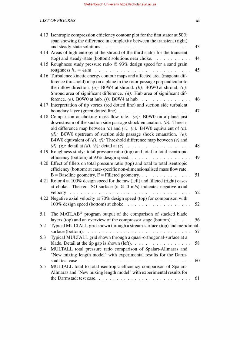
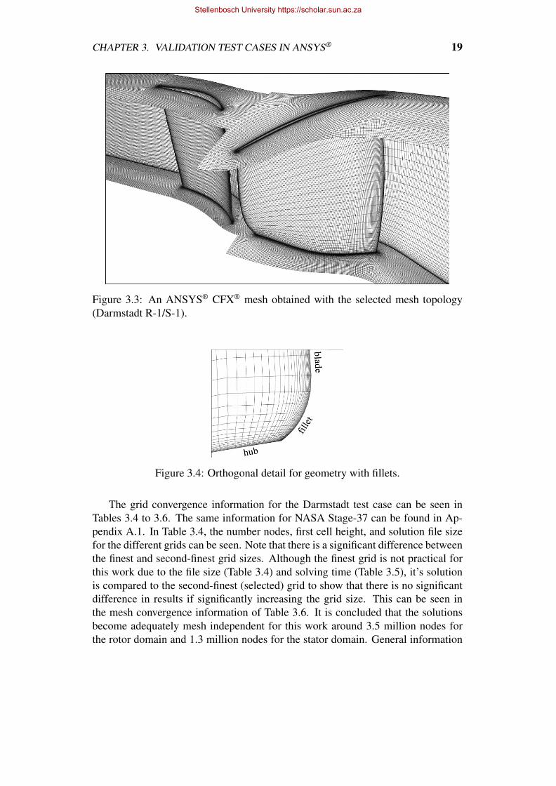
3.3 Mesh informationThe "Single Round Round Symmetric" O-type grid in ANSYS® CFX® is a sym-metric topology for single-bladed geometry with round leading and trailing edgesfor which refinement around the leading and trailing edges is not required. Thistopology is used for all simulations and is shown in Figure 3.2. An example of atypical mesh obtained with this topology is given in Figure 3.3. In the case of bladefillets, a shallow corner is added to the blade at the hub, as seen in Figure 3.4.
For both test cases, the grid spacing is relatively fine up and downstream of thecompressor stage in order to resolve the rotor-bow shock and the wake of stator stallseparation in high resolution.
Figure 3.2: Selected mesh topology for ANSYS® CFX® simulations.
Stellenbosch University https://scholar.sun.ac.za
CHAPTER 3. VALIDATION TEST CASES IN ANSYS® 19
Figure 3.3: An ANSYS® CFX® mesh obtained with the selected mesh topology(Darmstadt R-1/S-1).
Figure 3.4: Orthogonal detail for geometry with fillets.
The grid convergence information for the Darmstadt test case can be seen inTables 3.4 to 3.6. The same information for NASA Stage-37 can be found in Ap-pendix A.1. In Table 3.4, the number nodes, first cell height, and solution file sizefor the different grids can be seen. Note that there is a significant difference betweenthe finest and second-finest grid sizes. Although the finest grid is not practical forthis work due to the file size (Table 3.4) and solving time (Table 3.5), it’s solutionis compared to the second-finest (selected) grid to show that there is no significantdifference in results if significantly increasing the grid size. This can be seen inthe mesh convergence information of Table 3.6. It is concluded that the solutionsbecome adequately mesh independent for this work around 3.5 million nodes forthe rotor domain and 1.3 million nodes for the stator domain. General information
Stellenbosch University https://scholar.sun.ac.za

CHAPTER 3. VALIDATION TEST CASES IN ANSYS® 20
for the chosen grid sizes for Darmstadt R-1/S-1 and NASA Stage-37 can be foundin Table 3.7.
Table 3.4: General grid information (Darmstadt)
# Rotor nodes Stator nodesRotor first cellheight [um]
Stator first cellheight [um]
file size[GB]
1 1.2M 740k 20 20 1.662 1.55M 740k 20 20 1.943 2M 850k 20 20 2.424 3.1M 1M 20 20 3.495 3.1M 1M 10 10 3.546 3.4M 1.25M 5 5 3.937 21M 10.3M 0.15 0.35 25.9
Table 3.5: Residual convergence and solving speed (Darmstadt)
# W-mom V-mom U-mom P-Massiterations/s/thread
1 2.11E-04 9.74E-05 3.14E-04 1.32E-05 3.10E-032 1.95E-04 9.05E-05 2.93E-05 1.21E-05 2.75E-033 1.83E-04 8.70E-05 2.83E-05 1.22E-05 2.75E-034 1.54E-04 7.45E-05 2.57E-05 1.12E-05 1.47E-035 1.95E-04 9.95E-05 4.25E-05 1.27E-05 1.47E-036 1.98E-04 9.77E-05 4.28E-05 1.19E-05 1.38E-037 1.36E-04 7.34E-05 1.50E-04 2.82E-05 2.26E-04
Table 3.6: Grid y+ and convergence at choke (Darmstadt)
#Mass flow[kg/s]
Isentropicefficiency
Pressureratio
Rotor maxy+
Stator maxy+
1 16.445 0.70479 1.2859 29.6 21.72 16.462 0.7059 1.2865 29.6 21.63 16.46 0.7061 1.2865 30.0 22.34 16.465 0.7063 1.2864 30.0 22.35 16.475 0.70654 1.287 18.2 13.16 16.476 0.7065 1.287 11.2 7.87 16.486 0.7016 1.2822 1.19 0.856
Stellenbosch University https://scholar.sun.ac.za

CHAPTER 3. VALIDATION TEST CASES IN ANSYS® 21
Table 3.7: General grid information for chosen grid sizes.
Darmstadt R-1/S-1 NASA Stage-37Rotor domain elements 3.4 M 3.66 MStator domain elements 1.25 M 1.37 MMaximum rotor y+ 11.2 11.9Maximum stator y+ 7.8 9.8
3.4 Effect of transition modellingFrom Figure 3.5 it can be seen that, as expected, the transition onset moves down-stream as the grid y+ decreases. The flow images are of the stator, with the compres-sor stage operating at choking mass flow rate. The magenta ISO surface is one ofintermittency equal to 0.035, and intends to show the presence of laminar flow. Theboundary layer transition zone moves downstream until it reaches a passage shock.The shock interaction induces laminar separation. This shock-induced transition isnot to be confused with the transition region that is also found at lower mass flowrates in the same area due to large normal strain in the absence of a passage shock.Although the shock at the stator is of approximately the same strength for both theSST and SST − γReθ solutions, the shock does not affect the turbulent boundarylayer of the SST model as much as the laminar boundary layer of the SST − γReθmodel. In fact, the pre-shock Mach number reaches 1.3645 for the SST solution,whereas it reaches 1.355 for the SST − γReθ solution. The higher pre-shock Machnumber is most likely due to the thicker turbulent boundary layer produced by theSST model. This also means that the SST model predicts a lower choking massflow rate than the SST − γReθ model (16.47 kg/s as opposed to 16.40 kg/s). Thefact that transitional effects are physically present, and noting that turbulence mod-els with transition modelling predict a higher choking mass flow rate suggests thatthe choking mass flow rate predicted by the SST − γReθ may be more accuratethan that of other turbulence models due to over-predicted boundary layer blockagefor the assumption of fully turbulent flow.
Observing the rotor turbulence kinetic energy in Figure 3.6, it can be seen that,at choke and at half blade span, transition on the rotor occurs at mid-chord on thesuction side of the blade and near the trailing edge on the pressure side of the bladefor the SST − γReθ model. The thicker turbulent boundary layer of the SSTmodel also results in, for example, a 22% higher turbulent kinetic energy inducedinto the stator free stream by the mixing plane at this height. This also affects thestator boundary layer flow. Due to the extra mesh dependency of the SST − γReθturbulence model, all mesh dependency studies in this thesis are performed usingthis model.
The understanding gained thus far regarding the effects of transition modelingon compressor models is applied and expanded on during CFD validation and dur-
Stellenbosch University https://scholar.sun.ac.za

CHAPTER 3. VALIDATION TEST CASES IN ANSYS® 22
ing the transient and steady-state results-comparison.
Figure 3.5: Downstream movement of stator boundary layer transition with decreas-ing y+ in Darmstadt R-1/S-1 test case.
Figure 3.6: Rotor turbulent boundary layer comparison of SST − γReθ result (top)and SST result (bottom) at half span.
Stellenbosch University https://scholar.sun.ac.za

CHAPTER 3. VALIDATION TEST CASES IN ANSYS® 23
3.5 Motivation for using the SST − γReθ modelFollowing the mesh dependency study, the models were solved on the selected girds.Various turbulence models were used. The results for NASA Stage-37 are comparedto experimental results by Reid and Moore (1980) of NASA’s Lewis Research Cen-ter. The Darmstadt R-1/S-1 results are compared to experimental results by Mülleret al. (2007) and Bahktiari et al. (2015) of TU Darmstadt.
3.5.1 Darmstadt R-1/S-1 test caseThe Darmstadt performance curves of isentropic efficiency and overall pressure ra-tio are shown in Figure 3.7. Although it would seem that the k−ω turbulence modelproduces satisfactory results when observing these operating curves, the same can-not be said for the extent of expected stator flow separation on the stator. Theoperating point at which the oil streak lines of Figure 2.4 were allowed to settlein the stator during the experiment is unclear. The k − ω turbulence model failsto predict excessive flow separation on the stator near the operating point (Figure3.8.b), whereas the SST − γReθ model succeeds (Figure 3.8.a), but predicts irreg-ular overall performance results downward from 15.3 kg/s. The k − ε turbulencemodel produces results similar to the k − ω turbulence model, but with slightlyreduced separation. The SST turbulence model (no transition model) producesdisappointing results with regards to the change in efficiency with mass flow rate.
The shear stress limiting coefficient has been increased such that the numer-ical results from the SST − γReθ model is in closer agreement to the experi-mental performance curve and stator flow field separation behaviour. The SST −γReθ, a1 = 0.31 model predicts chaotic and highly unsteady stator flow separa-tion downward from 15.3 kg/s, with the hub corner stall region reaching 47% bladespan at a near stall mass flow rate of 15.3 kg/s, compared to 35% blade span forthe modified model. This is why the SST − γReθ, a1 = 0.31 model produces anunusual performance curve, as shown in Figure 3.7, which does not agree with theexperimental behaviour. A stator flow field comparison of the default and modifiedmodels at different mass flow rates (14.8, 15.2, 16 kg/s) is shown in Appendix A.3.It is concluded that the SST − γReθ turbulence model with modified shear stresslimiter (a1 = 0.345) is superior to the unmodified shear stress limiter (a1 = 0.31)with regards to predicting the experimental performance curve and the appropriatenature of flow separation on the stator. The reason for choosing (a1 = 0.345) isinfluenced not only by the Darmstadt results, but also the NASA Stage-37 results.Therefore, the shear stress limiting coefficient is discussed further in Section 3.6.
Although the k−ω turbulence model predicts flow separation near stall (Figure3.8.d), the structure of this separation does not agree well with experimental results.Comparing the orientation of shear lines for the two turbulence models at the shroudcorner separation (Figures 3.8.c and 3.8.d), it should be noted that the orientationof shear lines is inverted near the shroud for the k − ω turbulence model. A largerregion of negative axial velocity is observed near the shroud. From the experiment
Stellenbosch University https://scholar.sun.ac.za

CHAPTER 3. VALIDATION TEST CASES IN ANSYS® 24
it should be noted that the orientation of shear lines near the shroud agrees with thatof the SST − γReθ, a1 = 0.345 model. From the downward facing shear lines ofthe experiment and the SST − γReθ, a1 = 0.345 solution, it may be deduced thatthe experimental region of negative axial velocity for the shroud corner stall is incloser agreement with that of the SST − γReθ, a1 = 0.345 model. Furthermore,the k − ω turbulence model fails in predicting corner stall of adequate extent at thehub for the entire operating range (Figures 3.8.b and 3.8.d).
Figure 3.7: Darmstadt R-1/S-1 performance curves: isentropic efficiency (top),stage pressure ratio (bottom).
Stellenbosch University https://scholar.sun.ac.za

CHAPTER 3. VALIDATION TEST CASES IN ANSYS® 25
Figure 3.8: (a): SST − γReθ, a1 = 0.345 and (b): k − ω near peak efficiency(16 kg/s). (c): SST − γReθ, a1 = 0.345 and (d): k − ω near stall (14.8 kg/s).Red indicates regions of negative axial velocity. Numerical (e) and experimental (f)stator shear lines. The interpretation of experimental stator shear lines (g).
Stellenbosch University https://scholar.sun.ac.za

CHAPTER 3. VALIDATION TEST CASES IN ANSYS® 26
3.5.2 NASA Stage-37 test caseThe NASA Stage-37 performance curves can be found in Figure 3.9. For NASAStage-37, the k−ε and k−ω turbulence models yield results which seem superior tothose of the SST turbulence model, with or without a transition model. Additionalperformance curves for NASA Stage-37 can be found in Appendix A.4.
Figure 3.9: NASA Stage-37 performance curves: stage isentropic efficiency (top),stage pressure ratio (bottom).
Stellenbosch University https://scholar.sun.ac.za

CHAPTER 3. VALIDATION TEST CASES IN ANSYS® 27
Upon inspection of the flow field, it can be seen that a separation region causedby shock induced boundary layer separation on the suction side of the rotor bladeis far larger for the SST turbulence model than for the k − ε and k − ω turbulencemodels (Figure 3.10). Upon enabling the transition model, the size of this over-predicted separation region by the SST turbulence model decreases (Figure 3.10(c)), allowing the pressure ratio to increase.
The rotor bow-shock interacting with the suction side boundary layer is weakerfor the Darmstadt test case due to its higher pitch (fewer blades) and lower inlettip relative Mach number. The aspect ratio of the Darmstadt stage is such that therotor-bow shock intensity, which is also a function of distance from the emanation,decreases more severely along a spanwise hub to tip fraction in the direction ofthe hub. Additionally, adverse pressure gradient on the rotor blade suction sideboundary layer is less severe for the Darmstadt test case due to lower blade loading.This can be observed in the rotor blade loading charts of Figure 3.11.
Figure 3.10: Shock induced boundary layer separation at 20 kg/s on NASA Stage-37 rotor blade suction side. (a): SST , (b): SST − γReθ, a1 = 0.31 + ReattachmentProduction. (c): SST −γReθ, a1 = 0.31. (d): SST −γReθ, a1 = 0.345. (e): k−ω.(f): k − ε.
Stellenbosch University https://scholar.sun.ac.za

CHAPTER 3. VALIDATION TEST CASES IN ANSYS® 28
streamwise
0 0.2 0.4 0.6 0.8 1
stat
ic p
ress
ure
[kPa
]
0
50
100
150
200
250
50% blade height75% blade height
(a) NASA Stage-37
streamwise
0 0.2 0.4 0.6 0.8 1
stat
ic p
ress
ure
[kPa
]
0
50
100
150
200
250
50% blade height75% blade height
(b) Darmstadt R-1/S-1
Figure 3.11: Blade loading comparison at 50% and 75% blade height near operatingpoints (k − ω turbulence model).
Due to this weaker shock and adverse pressure gradient, the shock induced sep-aration is not sustained for the Darmstadt case, regardless of the turbulence model.For the Darmstadt case, the k − ω turbulence model predicts no shock inducedboundary layer separation. Minor shock induced boundary layer separation is pre-dicted by the SST −γReθ, a1 = 0.31 model, and reattachment occurs immediatelyafter the separation (Figure 3.12).
Figure 3.12: Darmstadt compressor near stall, showing minor shock induced bound-ary layer separation for the SST − γReθ model with a1 = 0.345.
Due to the significantly under-predicted pressure ratio by the SST and SST −γReθ, a1 = 0.31 models in the NASA test case, it becomes apparent that this is dueto over-predicted shock induced boundary layer separation on the blade suction sideof NASA Stage-37. However, as seen in the Darmstadt test case, the γReθ transitionmodel is required for the adequate flow behaviour in some regions of moderate
Stellenbosch University https://scholar.sun.ac.za

CHAPTER 3. VALIDATION TEST CASES IN ANSYS® 29
normal strain in the subsonic regime, such as the stator. Transition modelling isalso important for predicting the choking mass flow rate. The choking mass flowrate is influenced by boundary layer blockage and separation behaviour, both ofwhich are affected by transitional effects.
3.6 Adapting the shear stress limiterThe amount of shear stress in the boundary layer may be increased in order to re-duce flow separation. Noting that the SST turbulence model contains a shear stresslimiter, it might be possible solve this problem by reducing it’s effect. The limitercannot simply be disabled, since it is required for modelling the stator flow field.The amount of turbulent shear stress in the boundary layer can be controlled byvarying the structure parameter, a1. According to Tharwat et al. (2016), the SSTturbulence model performs well for mild adverse pressure gradients in subsonicflows and is designed to successfully predict separation where the majority of two-equation models fail to do so. Tan et al. (2011) states that, in some cases, the SSTturbulence model fails to accurately predict flow fields with strong shock/boundarylayer interaction (large normal strain). In the work by Tan et al. (2016), wherethe shear stress limiter strength is adapted to suit Mach 2.8 and Mach 5 experi-mental shock wave turbulent boundary layer interaction (SWTBLI) test cases, theyconclude that a constant value of stress limiter is not sufficient. Tan et al. (2011)hypothesises that the shear stress limiter could be made a function of the flow vari-ables and that more validation test cases are required.
Tharwat et al. (2016) mentions a recent SWTBLI workshop for a Mach 5 com-pression corner problem for which a value of a1 equal to 0.356 has been found ap-propriate. In the work of Tharwat et al. (2016) the standard SST turbulence modelover-predicts shock induced boundary layer separation in a dual throat nozzle prob-lem. A value of a1 equal to 0.34 was found to be appropriate in order to matchexperimental results. In the present work, a value for the structure parameter whichyields satisfactory results for both NASA Stage-37 and Darmstadt R-1/S-1 is to befound. The effect of this value on the overall performance of the client-specifiedmulti-stage compressor is investigated in Section 4.3 of the next chapter.
The structure parameter (a1) can be related to the shear stress limiting coeffi-cient, Clim, by
a1 =1
Clim
√β∗ (3.3)
where the model coefficient β∗ = 0.09. If Clim → 0, Menter’s SST turbulencemodel becomes the Menter BSL model, which is a predecessor of Menter’s SSTturbulence model. The SST turbulence model corresponds to Clim = 1. An elabo-rate discussion on the structure parameter can be found in Tharwat et al. (2016).
If the structure parameter is increased, the separated volume decreases (Figure3.10 (d)). As expected, this results in a higher pressure ratio. Note that a separationbubble of significant volume over the upper part of the blade, where higher blade
Stellenbosch University https://scholar.sun.ac.za

CHAPTER 3. VALIDATION TEST CASES IN ANSYS® 30
loading occurs, is eliminated. After comparing performance curves of the two dif-ferent test cases evaluated with values of a1 ranging from 3.3 to 3.7, it was decidedthat a value of a1 equal to 0.345 is adequate for both Darmstadt R-1/S-1 and NASAStage-37.
3.7 Concluding remarksWith the adapted shear stress limiter, adequate separation behaviour with regardsto flow structure is predicted on the Darmstadt stator, whilst suppressing seeminglypremature chaotic corner stall which starts at 15.3 kg/s for the unmodified model.Furthermore, the performance curves for both test cases are in close agreement withexperimental results.
For the Darmstadt test case and with the adapted shear stress limiter, the exper-imental (Müller et al., 2007) and numerical performance curves for stage pressureratio and stage isentropic efficiency differ by approximately 1.8% and 1.5% at theoperating point, respectively. In comparison to the experimental results by Bakhtiariet al. (2015), the stage pressure ratio and efficiency differ by approximately 0.1%and 2.0% at the operating point. For the NASA test case, the experimental (Reid& Moore, 1980) and numerical stage pressure ratio and stage isentropic efficiencydiffer by approximately 0.8% and 0.3%, respectively. It may be suggested thatthe value of a1 can be increased even more, since the experimental pressure ratiohas not yet been reached, and since the experimental Darmstadt stator shows lessseparation than the numerical solution. However, if it is increased by too much(for example a1 = 0.37), the isentropic efficiency of the Darmstadt compressor in-creases, shifting the numerical solution away from experimental results. It shouldbe kept in mind that surface roughness is not considered in the current test casestudy. Depending on the sensitivity of shock induced boundary layer separation tosurface roughness, further investigation might show that the numerical Darmstadtperformance curves move closer to experimental data while the numerical operatingcurves for the NASA case stay relatively constant due to the difference in numer-ically predicted shock induced separation between the two test cases. It is alsoconcluded that the appropriate value of the structure parameter in compressor CFDis case-specific.
Furthermore, it is concluded that the choking mass flow rate of a compressor isbetter predicted when a transition model is used. Results suggest that turbulencemodels without transition modelling over-predict blockage because of the omittedlaminar boundary layer flow present in the experiment.
Stellenbosch University https://scholar.sun.ac.za

Chapter 4
Main Numerical Investigation
In Section 4.1, the Darmstadt R-1/S-1 test case is considered for a comparison be-tween transient and steady-state results for a single stage. The insight gained is use-ful for doing a comparison between steady-state and transient overall performanceresults for the proprietary multi-stage compressor. The mesh dependency study forthis proprietary multi-stage compressor geometry is shown in Section 4.2, and thecompressor map is given in Section 4.3. To maintain confidentiality, all multi-stagecompressor results are non-dimensionalised with respect to a given design point.In Section 4.5, the effect of blade and endwall roughness on the proprietary multi-stage compressor is investigated. Lastly, the effect of blade fillets on the proprietarymulti-stage compressor is investigated in Section 4.6. In the current work, the ef-fects of fillets and surface roughness are studied in isolation.
4.1 Test case transient and steady-state comparisonFundamental differences between transient and steady-state results are investigatedin order to understand the significance of transient analysis at a steady operatingpoint (not near numerical stall).
The SST − γReθ model is used on a grid with a maximum stator y+ of 7.8. Asdiscussed in Section 2.5.2 and 3.4, although this is not ideal for the SST − γReθmodel, the model can still be used on this grid and the transition zone on this gridis close to the final location, which was shown by the y+max ∼ 1 solution. It is notthe purpose of this section to investigate particulars about the exact location of thetransition zone. For such an investigation, a maximum y+ value of ∼ 1 is required.Keeping in mind that the transient and steady-state comparison is also performedfor the multi-stage compressor, a grid with a maximum y+ value of ∼ 1 is notpractical for the current work.
In order to start with the fundamental differences, a single passage transientsolution at a single time step is compared to a steady-state mixing plane model.The models are solved at the choking mass flow rate in order to obtain a complexstator flow field.
31
Stellenbosch University https://scholar.sun.ac.za

CHAPTER 4. MAIN NUMERICAL INVESTIGATION 32
Since there are no time dependencies upstream of the rotor, no significant dif-ference in the rotor flow fields aside from upstream-travelling interactions from thestator is expected. Therefore, the investigation focuses on the stator flow field (Fig-ure 4.1).
Figure 4.1: Stator pressure side boundary layer flow field of the mixing plane model(top) and transient model (bottom). Featuring wall shear stress contours, a trans-parent ISO surface of negative axial velocity, and a magenta ISO surface of lowturbulence intermittency (0.035) to indicate the presence of nearby laminar flow.
A notable difference in the results is that the stator laminar boundary layer forthe transient solution extends toward the shroud, whereas it does not for the mixingplane model. This time dependency stems from the tip vortex structure, which isdestroyed by the mixing plane (Figure 4.2). For the transient model, time dependentpressure and shear variations occur at the stator shroud. At the hub, the first twonotable differences in the results are the presence of a turbulent boundary layerleading to a region of local high wall shear stress, and the joining of the laminar
Stellenbosch University https://scholar.sun.ac.za

CHAPTER 4. MAIN NUMERICAL INVESTIGATION 33
separation bubble with the end wall separation for the transient solution (Figure4.3).
Figure 4.2: The magenta ISO surface is of turbulence intermittency equal to 0.035to indicate the presence of nearby laminar flow. The transparent ISO surface showsnegative axial velocity.
The discrepancy between the mixing plane and transient models near the hub(Figure 4.3) is caused by a difference in the way in which the endwall boundarylayer is treated at the rotor-stator interface. For the transient solution, the turbulentboundary layer from the rotor domain is transferred directly to the stator domain,and the turbulent kinetic energy of this boundary layer is concentrated sufficientlyat the endwall to achieve local removal of the laminar boundary layer. This is shownin Figure 4.4. As the turbulent boundary layer approaches the stator laminar bound-ary layer, the turbulent kinetic energy is absorbed. If this dissipation is sufficient,the laminar boundary layer of the stator is locally removed, as is the case for thetransient solution (Figure 4.4 (c)).
Figure 4.3: The stator pressure side boundary layer flow field of the mixing planemodel (top) and transient model (bottom) showing two notable differences (dottedline).
For the mixing plane model, the turbulent kinetic energy from the rotor flowfield endwall boundary layer is dispersed, leading to a region of interaction thatspans a greater radial distance than for the transient solution. This higher free
Stellenbosch University https://scholar.sun.ac.za

CHAPTER 4. MAIN NUMERICAL INVESTIGATION 34
stream turbulent kinetic energy is the reason why the laminar separation bubbledoes not join with the endwall separation for the mixing plane solution , whereasit does for the transient solution. It is caused by thinning of the laminar boundarylayer for the mixing plane model for which the endwall turbulent kinetic energy isradially dispersed. The dispersion of turbulent kinetic energy over this region pre-vents separation close to the endwall, that would lead to the joining of the laminarseparation bubble and endwall separation. For this part of the laminar boundarylayer, transition can now occur without separation.
Figure 4.4: (a): Mixing plane model showing radial dispersion of endwall turbu-lent boundary layer turbulent kinetic energy. (b): Unconcentrated endwall turbulentboundary layer of mixing plane model fails to locally remove stator laminar bound-ary layer. (c): Concentrated endwall turbulent boundary layer of transient solutionlocally removes stator laminar boundary layer near endwall.
The boundary layer thickness in the applicable region is compared for the twomodels in Figure 4.5. For visual context, the location of the plane (12 cm from theaxis) used for Figure 4.5 can be seen in Appendix B.1.
A further difference in the results is that the mixing plane model velocity bound-ary layer starts at the leading edge of the hub, leading to high shear stress at the hubstator leading edge. This leads to higher pressure losses at the hub, causing a smallerstagnation point at the stator leading edge since the fluid has already been sloweddown. This is can be seen in Figure 4.6.
Stellenbosch University https://scholar.sun.ac.za

CHAPTER 4. MAIN NUMERICAL INVESTIGATION 35
Figure 4.5: Comparison of laminar boundary layer thickness. (a): Transient model.(b): Mixing plane model. (c): Difference between (a) and (b).
Figure 4.6: This figure illustrates the difference in wall shear (top half) and pres-sure (bottom half) distribution between the mixing plane (left) and transient (right)models.
In Figure 4.7, it can be seen that the rotor flow at the hub slows down priorto flowing over the non-rotating stator hub. This low momentum fluid (red ISOsurface of 10 m/s in Figure 4.7) joins with the rotor wake, and extends into thestator domain, creating stretched wall shear contours. This particular difference in
Stellenbosch University https://scholar.sun.ac.za

CHAPTER 4. MAIN NUMERICAL INVESTIGATION 36
the results is dependent on the rotor rotation-position relative to the stator at a fixedtime step.
Figure 4.7: Transient (top) and mixing plane (bottom).
It is apparent that the additional time dependencies inherent to the transient so-lution would have a significant effect on the transient results, when only consideringa single passage. This can be seen in Figure 4.8, which shows the time dependenttotal to total isentropic efficiency for a single and a multi-passage transient model.The multi-passage model has two rotor passages and three stator passages. Themodel is set up such that the rotor moves by one passage every 20 time steps (at de-sign speed, the resulting time step size is 9.375e-06 s). The variation in isentropicefficiency is more for a single-passage, with the signal period being 20 time steps,or one passage pass. Since a stage is normally designed to prevent resonance, therelative position of each rotor passage to that of a stator passage is unique whensolving at fixed time steps. This is why considering more passages is essential fortransient analysis, but makes no difference for steady-state mixing plane analysis.Due to the difference in relative rotor-stator positions, an irregular signal with alower amplitude is obtained. It is therefore likely that the amplitude will decreasefurther if more passages are considered.
Stellenbosch University https://scholar.sun.ac.za
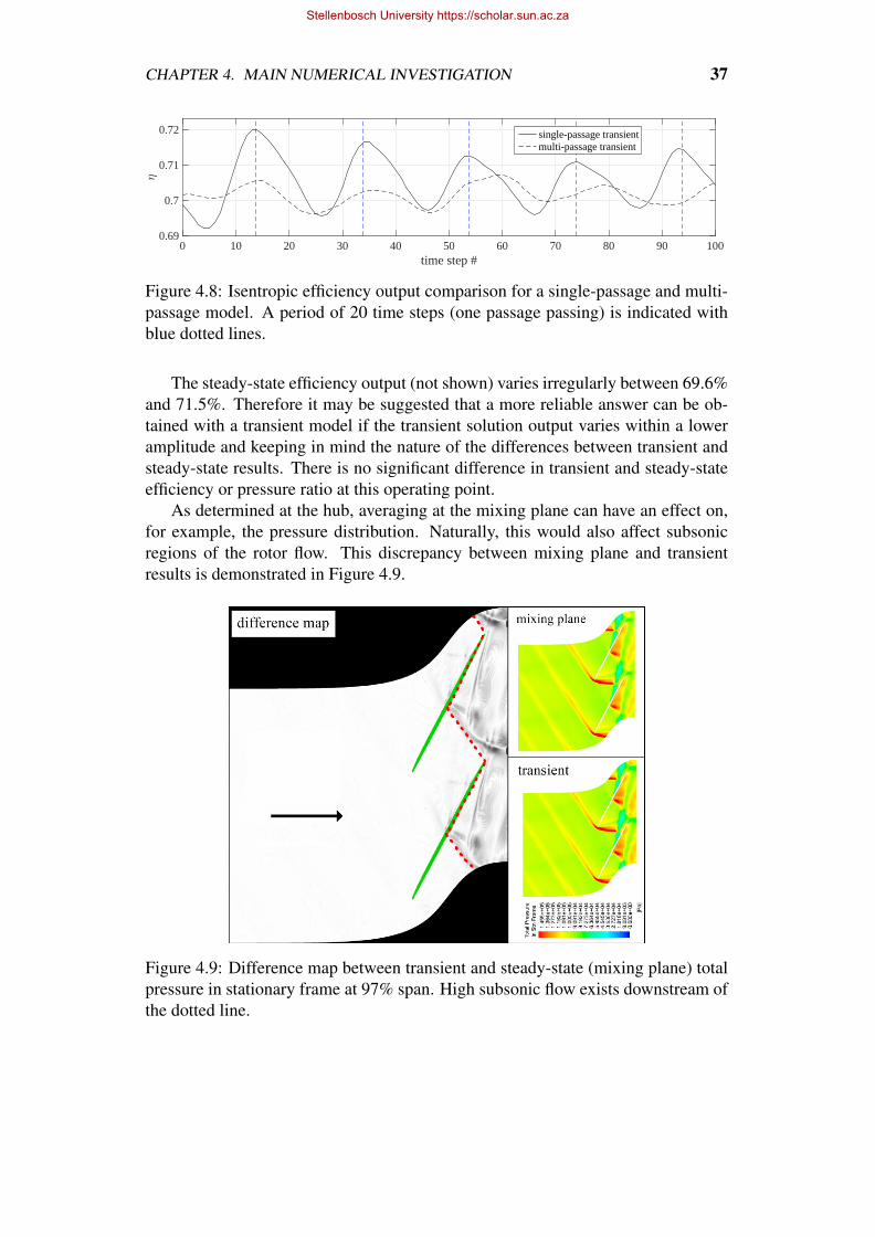
CHAPTER 4. MAIN NUMERICAL INVESTIGATION 37
time step #0 10 20 30 40 50 60 70 80 90 100
η
0.69
0.7
0.71
0.72 single-passage transientmulti-passage transient
Figure 4.8: Isentropic efficiency output comparison for a single-passage and multi-passage model. A period of 20 time steps (one passage passing) is indicated withblue dotted lines.
The steady-state efficiency output (not shown) varies irregularly between 69.6%and 71.5%. Therefore it may be suggested that a more reliable answer can be ob-tained with a transient model if the transient solution output varies within a loweramplitude and keeping in mind the nature of the differences between transient andsteady-state results. There is no significant difference in transient and steady-stateefficiency or pressure ratio at this operating point.
As determined at the hub, averaging at the mixing plane can have an effect on,for example, the pressure distribution. Naturally, this would also affect subsonicregions of the rotor flow. This discrepancy between mixing plane and transientresults is demonstrated in Figure 4.9.
Figure 4.9: Difference map between transient and steady-state (mixing plane) totalpressure in stationary frame at 97% span. High subsonic flow exists downstream ofthe dotted line.
Stellenbosch University https://scholar.sun.ac.za

CHAPTER 4. MAIN NUMERICAL INVESTIGATION 38
Lastly, since the output of each passage is unique due to a unique relative rotor-stator position, and since pressure waves can travel upstream toward the rotor pas-sage shock from the stator, variations occur between rotor passages. Figure 4.10shows the shift in pressure contour position between two neighbouring transientpassages. As expected, the most significant variations occur after the passage shock.
Figure 4.10: The shift in pressure contour position from one passage to the next at97% and 50% blade span.
4.2 Multi-stage compressor meshA mesh dependency study is performed on the proprietary multi-stage compressorgeometry. The mesh dependency study was performed at the choking mass flow rateand at 100% of the design speed, using the SST − γReθ turbulence model. Thestudy was also performed for a case with extreme relative Mach numbers throughoutthe compressor (115% of design speed) and a case with predominantly subsonicflow in the first 3 stages (70% of design speed), with the same conclusions. Theconsidered mesh sizes can be seen in Table 4.1. The change in mass flow rate, totalpressure ratio, and total to total isentropic efficiency relative to the result producedby the first mesh can also be seen in Table 4.1. It should be noted that the resultsfile size in Table 4.1 is for a single passage simulation. This is a post processingand storage space consideration, and is especially important for intermediate multi-passage transient results. The ratio at which the first cell height decreases through
Stellenbosch University https://scholar.sun.ac.za

CHAPTER 4. MAIN NUMERICAL INVESTIGATION 39
the respective stages compensates for the increase in y+. Due to the problem size,a mesh with a maximum y+ of ∼ 1 is not practical. It should also be kept in mindthat the solution is to be compared with a transient solution, which will considermultiple passages. Even though the maximum y+ on rotor-1 is 2.3 for the last mesh,the average y+ is 0.3. The average y+on stator-1 for this mesh is 0.2. The y+ valuesfor each rotor and stator can be seen in Table 4.2. The grid first cell height andthe attained convergence levels for continuity and mass conservation with a pseudotransient time step factor of 0.5 can be seen in Appendix B.2. It is concluded that thesolution becomes adequately mesh independent at a total of 8.33 million elements.
Table 4.1: General grid information and convergence
#Nodes/rotor
Nodes/stator
Totalnodes
Totalelements
Size[GB]
m πtot ηtot
1 220-270 k 180 k 1.70 M 1.56 M 1.55 1.0000 1.0000 1.00002 360-430 k 220 k 2.43 M 2.26 M 2.21 1.0020 0.9681 0.95783 370-460 k 220 k 2.55 M 2.37 M 2.31 0.9977 1.0023 1.02444 490-620 k 220 k 3.15 M 2.95 M 2.83 0.9952 0.9580 0.98625 700-870 k 280 k 4.23 M 4.00 M 3.80 0.9948 0.9868 1.01606 0.95-1.17 M 330 k 5.60 M 5.34 M 5.00 0.9960 0.9654 0.98147 0.95-1.17 M 440 k 6.05 M 5.77 M 5.38 0.9963 0.9796 0.99548 1.47 M 630 k 8.68 M 8.33 M 7.68 0.9968 0.9556 0.95929 1.75 M 630 k 9.94 M 9.58 M 8.76 0.9963 0.9524 0.959410 2.3 M 830 k 13.15 M 12.73 M 11.56 0.9962 0.9589 0.9594
Table 4.2: Grid y+ for per rotor / stator
#max y+
rotor-1max y+
rotor-2max y+
rotor-3max y+
rotor-4max y+
stator-1max y+
stator-2max y+
stator-3max y+
stator-4
1 103 112 120 120 96 132 135 1282 111 114 123 123 98 141 140 1333 61 63 64 77 55 76 71 694 34 34 35 38 30 6 37 365 18 19 19 21 16 20 19 196 19 20 19 21 17 21 19 197 19 20 19 21 17 21 19 198 11 12 11 12 9 11 10 109 4.2 4.1 4.3 4.4 2.5 2.7 2.5 2.310 2.3 2.4 2.5 2.6 1.1 1.1 1.1 1
Stellenbosch University https://scholar.sun.ac.za

CHAPTER 4. MAIN NUMERICAL INVESTIGATION 40
4.3 Baseline multi-stage compressor mapThe baseline (no surface roughness, no fillets) compressor speedlines in Figure 4.11were simulated such that the CFD model stalled to the nearest 1 kPa of the variedstatic pressure outlet. This means there is variability in terms of closeness to nu-merical stall inception of each speedline. This also means that it may be possibleto obtain solutions at lower mass flow rates for each speedline by searching for thepoint of stall inception using smaller increments of static outlet pressure. Whennumerical stall is reached, the mass flow rate becomes unstable in the time domainand decreases toward 0, with the solution diverging before this can happen. Thek − ω turbulence model, which is also required for the roughness comparison, isused for the baseline compressor map simulation, keeping in mind the number ofsolutions and the fact that it is a single-passage mixing plane simulation. The k−ωturbulence model performed well with regards to overall performance in the testcases.
4.3.1 Discussion of resultsIn the test cases it was seen that the k − ω model produces a solution with a lowerchoking mass flow rate than the SST − γReθ model, even though more flow sep-aration is observed with the SST − γReθ model due to the shear stress limiter.In the test cases, the laminar boundary layer flow present on the rotor and statorfor the SST − γReθ compensated for the increased flow separation, reducing theblockage. In a multi-stage compressor the flow is highly turbulent downstream ofthe first stage, leading to negligible areas of laminar boundary layer flow in down-stream stages. This is why the choking mass flow rate is more rather than less whencomparing a k − ω and a SST − γReθ solution for the multi-stage compressor atdesign speed. This is not the case for 93% speed, at which less flow separationis observed. When comparing the SST − γReθ and SST solutions, the transitionmodel reduces corner stall. This was also seen during CFD validation. The transi-tion model allows for significant laminar boundary flow in the first stage. At designspeed, the choking mass flow rate of the SST − γReθ solution is 0.2% less thanthat of the k−ω solution. If the shear stress limiting coefficient of the SST −γReθmodel is increased from 0.31 to 0.345, areas of separation decrease such that thechoking mass flow rate is only 0.05% less than that of the k−ω solution. The SST(no transition model) solution choking mass flow rate is 0.6% less than that of thek − ω solution. During CFD validation it was concluded that the SST model mostlikely over-predicts flow separation and therefore blockage. At 93% shaft speed, thechoking mass flow rate of the SST − γReθ solution is still 0.2% less than that ofthe k − ω solution, but as in the validation test cases, the choking mass flow rate ofthe SST −γReθ model with a1 = 0.345 is now more than that of the k−ω solution(+0.33%). This is because the blockage is less dependent on flow separation whenreducing the shaft speed from 100% speed where flow separation is rather signifi-cant. This is analogous to what is observed during the roughness investigation.
Stellenbosch University https://scholar.sun.ac.za

CHAPTER 4. MAIN NUMERICAL INVESTIGATION 41
Figu
re4.
11:M
ulti-
Stag
eco
mpr
esso
rspe
edlin
es(k−ω
turb
ulen
cem
odel
).
Stellenbosch University https://scholar.sun.ac.za

CHAPTER 4. MAIN NUMERICAL INVESTIGATION 42
A comparison of the k− ω and SST − γReθ, a1 = 0.345) results at 93% speedcan be seen in Figure 4.12. The mass flow rate of the performance curves of Figure4.12 are non-dimensionalised with respect to the choking mass flow rate of theSST − γReθ, a1 = 0.345 solution.
m/mCh
0.96 0.97 0.98 0.99 1
ηto
t/ηto
t D
0.6
0.7
0.8
0.9
1
1.1
k-ωSST-γRe
θ, a
1= 0.345
m/mCh
0.96 0.97 0.98 0.99 1
πto
t/πto
t D
0.5
0.6
0.7
0.8
0.9
1
k-ωSST-γRe
θ, a
1= 0.345
Figure 4.12: Comparison of k−ω and modified SST −γReθ solution performancecurves at 93% speed (not simulated to numerical stall) showing isentropic efficiency(top) and stage pressure ratio (bottom).
With regards to pressure ratio, the k − ω and SST − γReθ, a1 = 0.345 so-lutions show similar results, with the SST and SST − γReθ, a1 = 0.31 mod-els showing reduced blade loading, but similar or slightly higher (+0.35% for theSST−γReθ, a1 = 0.31 model) total to total isentropic efficiency. This is analogousto what was observed for the test cases. At 93% speed, maximum pressure ratio ofthe SST − γReθ, a1 = 0.345 solution is only 0.8% less than that of the k−ω solu-tion. In contrast to this, the predicted pressure ratio by the SST − γReθ, a1 = 0.31
Stellenbosch University https://scholar.sun.ac.za

CHAPTER 4. MAIN NUMERICAL INVESTIGATION 43
model is 6.2% less than that of the k − ω solution. Similar to what was observedduring the NASA test case, for which strong shock-interactions also occur, thissignificant difference is due to a reduction in suction-side shock-induced boundarylayer separation when increasing the shear stress limiter. Following the conclusionsof the test cases, the k − ω solution and the SST − γReθ, a1 = 0.345 solutionshould best match physical results.
4.4 Multi-stage transient and steady-statecomparison
Continuing from the test case transient and steady-state comparison of Section 4.1,a comparison is performed on the proprietary multi-stage compressor at the designpoint and at an off design operating point with the SST − γReθ model on theselected grid. It is not practical to consider a grid with a y+ value of ∼ 1 for thissimulation because the solving time would not be justifiable when keeping in mindthat it is not the purpose of this investigation to solve for a high-fidelity solution(no fillets, no surface roughness). In this transient multi-passage simulation, 3 rotorpassages and 5 to 6 stator passages are considered. An example of the difference incomplexity between transient and steady-state results due to rotor-stator interactionby means of a contour plot of isentropic efficiency can be seen in Figure 4.13. Thecomplete figure is given in Appendix B.3.
Figure 4.13: Isentropic compression efficiency contour plot for the first stator at50% span showing the difference in complexity between the transient (right) andsteady-state solutions
In Section 4.1, it was seen that although the transient and steady-state perfor-mance results do not vary within the same limits, the difference is not significantfor the Darmstadt test case. However, in a single-stage simulation there is only onemixing plane. The difference may be more significant in multi-stage compressors,which have two mixing planes per stage and keeping in mind that the error is boundto be cumulative. Losses from secondary flow across rotor-stator interfaces are notproperly accounted for when using a mixing plane. Pullan (2004) found that 10%less losses were produced by a steady-state model when compared to a transientmodel of a turbine stage. Figure 4.14 shows an example of increased areas of highentropy at the stator of the third stage due to the rotor tip leakage flow. At bothoperating points, the peak static entropy is more than 15% higher for the transient
Stellenbosch University https://scholar.sun.ac.za

CHAPTER 4. MAIN NUMERICAL INVESTIGATION 44
case. This is most likely due to the difference in the transfer of the tip leakage flowacross the interface.
Figure 4.14: Areas of high entropy at the shroud of the third stator for the transient(top) and steady-state (bottom) solutions near choke.
At the design point, the isentropic efficiency drops by 1% for the proprietarymulti-stage compressor. The pressure ratio drops by 0.9%. At a point near choke,the isentropic efficiency drops by 3.7%, and the pressure ratio drops by 2.3%. Ameridional analysis with circular averaging can be used to show that the entropyproduction at the hub is more for the transient model. Increased entropy at thehub can be seen for the steady-state case in rotors 1 and 3 due to increased cornerstall. Differences in flow separation are observed due to, for example, the way inwhich turbulent kinetic energy is transferred across the interface, which affects theboundary layer flow as observed during the Darmstadt comparison of transient andsteady-state results (Section 4.1). The transient simulation shows thicker boundarylayer flow due to the proper transfer thereof at the interface. The choking mass flowrate is 1.2% less for the transient model.
4.5 Effect of blade and endwall roughnessThe roughness investigation was carried out at 93% and 100% speed on the base-line (no fillet) geometry, using the k − ω turbulence model. Roughness modellingwith the SST − γReθ model would require performing test cases for roughnessvalidation. In the current work, the roughness height is defined by the sand grainroughness. Sand grain roughness (hs) values of 1, 4 and 8 µm were tested on theblades and on the casing, resulting in 9 combinations, as per the graph legends.
Stellenbosch University https://scholar.sun.ac.za

CHAPTER 4. MAIN NUMERICAL INVESTIGATION 45
Sand grain roughness between 1 and 8 µm in a compressor can account for surfaceroughness due to manufacturing and fouling (Chinnaswamy, 2015).
First, the results at 93% speed are discussed, since the 100% speed results lackmass flow stall margin, and one would therefore not be able to investigate muchmore than the effect on choking mass flow rate. For sand grain roughness of 4µm,the performance curves were evaluated towards numerical stall until the numericalmodel stalled to the nearest 500 Pa of varied static pressure outlet. This is also thecase for the smooth surface (B0W0) model. Figure 4.15 shows the total pressureratio as affected by blade and wall roughness of hs = 4µm. B4 refers to bladeroughness of hs = 4µm and W0 to wall roughness of hs = 0µm (smooth surface),and so forth. Results at 100% speed can be found in Appendix B.4.
m/mch.s
0.93 0.94 0.95 0.96 0.97 0.98 0.99 1
πto
t/πto
t D
0.86
0.88
0.9
0.92
0.94
0.96
0.98
1
1.02
1.04
1.06
B0W0B0W4B4W0B4W4
Figure 4.15: Roughness study pressure ratio @ 93% design speed for a sand grainroughness hs = 4µm
As expected, the choking mass flow rate decreases as the total roughened surfacearea through the compressor increases due to increased blockage. However, notethe crossover near 99% of the smooth surface choking mass flow rate (B0W0 vsB0W4 and B4W0 vs B4W4) when the blade roughness is kept constant and thewall roughness increased. A higher pressure ratio is observed when wall roughnessis added, regardless of whether the blades are roughened. It may be explained usingpassage plots on a plane perpendicular to the flow. Figure 4.16 shows the turbulentkinetic energy at the hub and a portion of the blade.
Stellenbosch University https://scholar.sun.ac.za

CHAPTER 4. MAIN NUMERICAL INVESTIGATION 46
Figure 4.16: Turbulence kinetic energy contour maps and affected area (magentadifference threshold) map on a plane in the rotor passage perpendicular to the in-flow direction. (a): B0W4 at shroud. (b): B0W0 at shroud. (c): Shroud area ofsignificant difference. (d): Hub area of significant difference. (e): B0W0 at hub.(f): B0W4 at hub.
From Figure 4.16 (d) to (f), it can be seen that the turbulent boundary layer atthe hub is larger for the B0W4 case, while the rotor turbulent boundary layer isunchanged. From (a) to (c) it should be noted that the area of high turbulent kineticenergy on this image is larger for the B0W0 case, in contrast to what is seen atthe hub. This is because of a smaller tip leakage flow for the B0W4 case, causedby blockage of the tip vortex gap by means of a thicker casing boundary layer.Due to the angle at which the tip vortex intersects the plane, the tip vortex should
Stellenbosch University https://scholar.sun.ac.za

CHAPTER 4. MAIN NUMERICAL INVESTIGATION 47
be interpreted as depicted in Figure 4.17. It does not form part of the turbulencekinetic energy migrating towards the shroud from the suction side surface (greendotted line). As expected, the rotor boundary layer size is unaffected. If the hub andshroud boundary layer size confines the flow path, and with less tip gap losses andat the same rotational speed (not the same shaft power), the pressure ratio increasesas per Figure 4.15.
Figure 4.17: Interpretation of tip vortex (red dotted line) and suction side turbulentboundary layer (green dotted line).
Using contour plots of velocity magnitude in the stationary reference frame, itwas confirmed that the casing boundary layer in the tip gap is indeed thicker for therough wall case. This is not surprising (and therefore not shown) since roughnessmodelling is based on Nikuradse’s shifting of the logarithmic law of the wall.
Considering Figure 4.15 near choke, it can be seen that the addition of bladeroughness has a significant effect on the choking mass flow rate when comparedto the addition of endwall roughness. This is expected because the blade consti-tutes the majority of the passage outline when observing a blade passage from thedirection perpendicular to the flow and would naturally cause more blockage (Fig-ure 4.18). However, blockage at the shroud is also affected by the blade suctionside turbulent boundary layer migrating towards the casing and mixing with the tipclearance flow (Figure 4.17 and 4.18). The reduced tip clearance vortex size in thecase of a roughened shroud compensates for some of the blockage caused in thatcase. It should also be noted that, in the case of a roughened blade, the tip clearanceblockage is also increased due to roughness on top of the blade. However, the tipclearance vortex joins directly with the thickened migrating suction side boundarylayer. This worsens the situation because the low-momentum flow accompanyingthe tip clearance vortex is now more rather than less. This explains the significantdifference between the effect of endwall and blade roughening on the choking massflow rate.
Stellenbosch University https://scholar.sun.ac.za

CHAPTER 4. MAIN NUMERICAL INVESTIGATION 48
Figure 4.18: Comparison at choking mass flow rate. (a): B0W0 on a plane justdownstream of the suction side passage shock emanation. (b): Threshold differencemap between (a) and (c). (c): B4W0 equivalent of (a). (d): B0W0 upstream ofsuction side passage shock emanation. (e): B4W0 equivalent of (d). (f): Thresholddifference map between (e) and (d). (g): detail at (d). (h): detail at (e).
At 100% speed, the effect of roughness on the choking mass flow rate is lessthan at 93% speed. The decrease in peak efficiency for the extreme case (B8W8)is less than 1% at design speed, and just under 1.5% at 93% design speed. Thepressure ratio decreases by over 3% for the extreme case at 93% speed. It can beconcluded that the compressor is much more sensitive to blade roughness than end-wall roughness, and it is most likely most sensitive to blade suction side roughnessdue to the observed significantly thickened suction side boundary layer. Figure 4.19shows the pressure ratio and efficiency for all cases at 93% speed.
Stellenbosch University https://scholar.sun.ac.za

CHAPTER 4. MAIN NUMERICAL INVESTIGATION 49
m/mch.s
0.93 0.94 0.95 0.96 0.97 0.98 0.99 1
πto
t/πto
t D
0.86
0.88
0.9
0.92
0.94
0.96
0.98
1
1.02
1.04
1.06
B0W0B0W1B0W4B0W8B1W0B4W0B8W0B1W1B4W4B8W8
m/mch.s
0.93 0.94 0.95 0.96 0.97 0.98 0.99 1
ηto
t/ηto
t D
1.035
1.04
1.045
1.05
1.055
1.06
1.065
1.07
1.075
1.08
1.085B0W0B0W1B0W4B0W8B1W0B4W0B8W0B1W1B4W4B8W8
Figure 4.19: Roughness study: total pressure ratio (top) and total to total isentropicefficiency (bottom) at 93% design speed.
Stellenbosch University https://scholar.sun.ac.za

CHAPTER 4. MAIN NUMERICAL INVESTIGATION 50
4.6 Effect of blade filletsUsing a mesh of the same size as the baseline investigation, an investigation on theeffect of blade fillets is carried out using the k − ω turbulence model. Figure 4.20shows the results. The mass flow rates are non-dimensionalised according to thebaseline choking mass flow rate for each shaft speed.
Surprisingly, the mass flow rate increases if fillets are applied at 100% and 93%speed at choke. The original mesh convergence was re-evaluated and confirmed byrunning one operating point with a courser and finer mesh. It was also confirmedthat the same conclusions are applicable with the SST−γReθ by running one pointon each speedline and comparing the result to the baseline SST − γReθ results.The reason for increased choking mass flow rate is that the blockage through thecompressor is highly dependent on hub corner stall around the design point. Theadded material blockage (by means of fillets) is more than compensated for by asignificant reduction in flow separation. Figure 4.21 shows an example of this.Another example can be found in Appendix B.5. At 70% speed however, flowseparation in the baseline compressor flow field is much less (Figure 4.22) and thefillets only add to the blockage, reducing the choking mass flow rate. At 70% shaftspeed, the pressure ratio and insentropic efficiency clearly decrease when fillets areadded. This is most likely due to reduced flow turning at the hub and enhancedsecondary flow losses as stated by Shi et al. (2010). Shi et al. points out that theadded fillet thickness at the point of maximum blade thickness pushes the flow nearthe hub radially outwards. This secondary flow mixes with the free stream, whichincreases losses. In the case of non-axisymmetric edges of blade rows due to evenover-sized fillets, the pressure ratio and mass flow rate would most likely fluctuatedue to time-dependent material blockage. The compressor could also experience anincrease in time-dependent secondary flow losses and vibration.
At 93% shaft speed and away from choke, the compressor blockage becomesless dependent on corner stall since the corner stall decreases away from choke, andthe mass flow rate subsequently decreases with the addition of fillets. The pressureratio is less affected at 93% speed. This is due to corner stall compensation, sinceboth corner stall and fillets reduce the flow turning and therefore blade loading(corner stall is replaced by material blockage by means of fillets). This explainswhy the drop in pressure ratio is more significant at 70% speed, where there is littlecorner stall to begin with.
Interestingly, the isentropic efficiency is increased rather than reduced in thecase of fillets for 93% speed. However, the required shaft power at the same pres-sure ratio is 1.6% more for the filleted model. This is because the effect of stagna-tion, which is a loss in terms of fluid flow, is replaced by material blockage. Onceagain, this is not the case for 70% speed where there is little flow separation to beginwith.
Stellenbosch University https://scholar.sun.ac.za

CHAPTER 4. MAIN NUMERICAL INVESTIGATION 51
m/mCh
0.95 0.96 0.97 0.98 0.99 1
πto
t/πto
t D
0.2
0.4
0.6
0.8
1B - 100%F - 100%B - 93%F - 93%B - 70%F - 70%
m/mCh
0.95 0.96 0.97 0.98 0.99 1
ηto
t/ηto
t D
0.5
0.6
0.7
0.8
0.9
1
1.1
1.2
B - 100%F - 100%B - 93%F - 93%B - 70%F - 70%
Figure 4.20: Effect of fillets on total pressure ratio (top) and total to total isen-tropic efficiency (bottom) at case-specific non-dimensionalised mass flow rate. B =Baseline geometry, F = Filleted geometry.
Stellenbosch University https://scholar.sun.ac.za

CHAPTER 4. MAIN NUMERICAL INVESTIGATION 52
Figure 4.21: Rotor 4 at 100% design speed for the raw (left) and filleted (right)cases at choke. The red ISO surface (u @ 0 m/s) indicates negative axial velocity
Figure 4.22: Negative axial velocity at 70% design speed (top) for comparison with100% design speed (bottom) at choke.
Stellenbosch University https://scholar.sun.ac.za

Chapter 5
MULTALL
MULTALL-open is a rapid turbomachinery design suite of programs. Three pro-grams can be found within MULTALL-open. MEANGEN can be used in a rapidinitial design process. MEANGEN generates an input file for STAGEN. The STA-GEN input file provides the essential compressor geometry and mesh definition, aswell as boundary conditions and initial solution guesses. An input file to MULTALLcan be generated in a matter of minutes. A 3D simulation can then be performedin MULTALL. According to Denton (2017), a typical MULTALL simulation con-verges in the order of 15 minutes per stage (computing speed is not mentioned). Inthe current work MULTALL-open is used for turbomachinery analysis rather thanfor its intended purpose, which is turbomachinery design.
5.1 MULTALL as an analysis toolFor the purpose of analysing an existing compressor, STAGEN can be used as astarting point. Once the STAGEN input file is completed, the blade profiles may beplotted. If the user is satisfied with the profile plots, STAGEN generates an inputfor MULTALL. In STAGEN, all blade rows must be defined in an equal number ofspan-wise sections (this may be an inconvenience). The STAGEN input file maybe used to add lean and sweep to the blades, as well as axial positioning of theblades without manually modifying the coordinates. This is convenient for a rapidcomparison of different designs within these design parameters. The geometry canalso be scaled in specific ways within STAGEN. However, it will be seen that, insome cases, STAGEN warps the geometry and that it is better to perform thesealterations with an external program, written for example, in MATLAB®. STAGENdoes not provide a means for a complete definition of the geometry, such as definingaxial variation in tip clearance gap or defining blade fillets. However, these aspectsof the geometry can be defined by modifying the MULTALL input file coordinates.Fillet geometry can only be introduced by adding more profile sections at the filletas a means of defining it. Since STAGEN is a design program, it decides aboutcertain aspects of the geometry or computational domain by itself. This may lead
53
Stellenbosch University https://scholar.sun.ac.za

CHAPTER 5. MULTALL 54
to inaccuracies when using STAGEN to input existing geometry.
5.2 MULTALL geometry defintionThe way in which existing geometry was recreated in MULTALL format for thetest cases and for the multi-stage compressor is discussed. In the current work, theMULTALL geometry is defined using the input file to STAGEN, as well as mod-ification of the subsequently generated MULTALL input file. When defining thegeometry, the user may consult "Instructions for Program STAGEN" by Denton(2017). The available methods in STAGEN that are most convenient when consid-ering the geometry format were attempted. During the test case geometry input,the process was found to be tedious due to unexpected warping of the geometry bySTAGEN. However, during the multi-stage geometry input, a promising solution tothis problem was found.
5.2.1 Test case geometryUsing MATLAB®, coordinates were reproduced or interpolated as needed beforebeing written into the appropriate format in order to compile the STAGEN inputfile. Such an input file formatted for a coordinate-based input method and definingthe geometry for one stage, typically consists of roughly 2000 rows with multipleentries per row.
The blade geometry was oriented according to the convention commonly usedin MULTALL using the appropriate rotation settings in the STAGEN input file. Theresults from the initial simulation, which used a coordinate-based blade definition,greatly differed from what was expected. Upon inspection of the results and of theprograms, it was found that STAGEN displays the correct blade profiles for perusalby the user, but distorted the output geometry when it produced the MULTALLinput file.
According to Denton (2017), the standard means of defining blade geometryin MULTALL is by a blade angle distribution as a function of blade chord, with amathematically defined thickness distribution. In this method, the user inputs cer-tain constants, which STAGEN uses to calculate the thickness distribution. Dueto the peculiar results when using the coordinate method, this blade-angle andthickness-distribution-method was attempted next. MATLAB® was used to cal-culate these parameters from the blade coordinates. STAGEN could be used toplot thickness distribution graphs of the original blade coordinates. The thicknessdistribution of the new blade data was then iteratively matched to that of the orig-inal blading by means of the mathematical thickness distribution. The parametersfor defining a thickness distribution in STAGEN do not provide complete freedom,however, the difference between the new and original blading is, in most cases,small. To illustrate what is meant by this, a comparison between the original andmathematically-defined thickness distribution is shown in Appendix C.1.
Stellenbosch University https://scholar.sun.ac.za

CHAPTER 5. MULTALL 55
A compromise must be made between the accuracy of the leading or trailingedge thickness and the accuracy of the geometry around the point of maximumthickness. Emphasis was placed on the accuracy of the thickness distribution aroundthe point of maximum thickness. In either case, the shock structure will be affected.Aside from the obvious difference in choking mass flow if the maximum thicknessis not accurate, it is assumed that the shock structure may be more significantly af-fected with regards to shock position if the geometry around the point of maximumthickness, where the thickness distribution does not change as abruptly as a functionof chord position, is not as accurate as possible.
Unless a program that interpolates and converts coordinates directly into a de-sired mesh in the format required by MULTALL is written, it is likely that thegeometry produced by STAGEN will always contain discrepancies.
In some cases, the pitch-wise dimension of the blade profiles is extended bySTAGEN, which also results in incorrect blade angles. There is no direct constraint-control over this dimension. Before generating a MULTALL input file, STAGENfits the approved blade profiles between leading and trailing edge coordinates whichcan be defined in the radial and axial coordinates. It is apparent that the pitch-wisedimension can be calculated through the blade angle and these coordinates, yet thegeometry is often warped such that these geometric relations no longer hold true.The geometry cannot be viewed in MULTALL nor STAGEN.
Even if the geometry is not warped, the geometry for a compressor may bedefined with blade profiles which are not aligned with streamlines and at the huband shroud surface, as is required by STAGEN. It is often the case that a profileis defined as extending from inside the hub or outside the shroud. In such cases,writing the STAGEN input file requires prior interpolation of blade coordinates,perhaps along a section that is irregularly shaped at the hub or shroud. Creatinga STAGEN input file that exactly satisfies the geometry format requirements is, inmost cases for existing geometry based on coordinate measurement, not practicalbecause it is too time-consuming. It therefore becomes clear that, regardless of thediscrepancies and regardless of the reason for often warped geometry, and keepingin mind the inability to view the geometry within the MULTALL open-source suiteof programs, a program should be written with which the geometry can be viewedin the MULTALL format and validated against the original format.
A MATLAB® program which finds and plots the appropriate coordinate datawithin the MULTALL input file was written. It can also be used to plot the origi-nal profile data. With the discrepancies in mind, the program was written such thatblade profiles can be (non-uniformly) scaled and translated to alleviate discrepan-cies in blade angles. Due to possible discrepancies in thickness and blade turningas a result of off-set blade profile sections (such as a profile section defined fromwithin the hub), the profile thickness can be changed. The camber of a profile canbe changed by multiplying a fraction of a non-dimensionalised thickness distribu-tion with the blade coordinates. This may have an unwanted thinning-effect on theleading and trailing edge thickness, therefore a decaying function is used to addthickness to the leading and/or trailing edge if needed. A typical example of the
Stellenbosch University https://scholar.sun.ac.za

CHAPTER 5. MULTALL 56
graphical output by the program can be seen in Figure 5.1. Using a top view, theMULTALL blade profiles are adjusted to fit the measured geometry.
Figure 5.1: The MATLAB® program output of the comparison of stacked bladelayers (top) and an overview of the compressor stage (bottom).
5.3 Multi-stage compressor geometryAlthough it is clear that MULTALL, in its current version, is far from ideal for ex-isting geometry, importing the geometry of the multi-stage compressor was muchless effort per compressor stage than the CFD test cases. This is because of a dif-ferent geometry definition option in STAGEN and because of the way in whichparticulars of the multi-stage compressor, which was created by ANSYS® CFX®’snative turbomachinery tools, could be exported. STAGEN offers an option to defineblade layers by means of angles and tangential thickness distribution as a functionof blade chord. This option is attractive because the axial thickness distribution andthe leading, trailing, and mid-chord blade angles could be exported from ANSYS®
CFX®. It was only needed to convert the axial thickness distribution to tangentialthickness distribution. In order to do this, vectors of blade angles correspondingto the irregularly-spaced axial thickness distribution-vectors were interpolated. The
Stellenbosch University https://scholar.sun.ac.za

CHAPTER 5. MULTALL 57
tangential thickness distribution as a function of blade chord could then determined.In this format, it is far less time-consuming than iteratively matching the mathemat-ical thickness distribution, as done for the test case geometry definition. Further-more, a significant advantage is that STAGEN did not warp the geometry such thatblade angles or blade thickness was changed. Although the dimensions of the pro-files were accurate, STAGEN straightened the forward-lean of the rotor blades andmoved some profiles such that the spacing between profiles at the mixing-planebecomes larger. Therefore, using this method of geometry definition, only the posi-tion of blade profile layers relative to each other is changed. This was corrected byusing the MATLAB® program. Although a larger spacing at the mixing plane canassist with convergence, the manner in which the position of the stacked profileswas changed relative to each other was not accurate. Therefore the profiles weremoved to their original position.
5.4 MULTALL Modelling setupMULTALL uses H-grid topology. A typical example of a typical MULTALL gridcan be seen in Figures 5.2 and 5.3.
Figure 5.2: Typical MULTALL grid shown through a stream-surface (top) andmeridional-surface (bottom).
Stellenbosch University https://scholar.sun.ac.za

CHAPTER 5. MULTALL 58
Figure 5.3: Typical MULTALL grid shown through a quasi-orthogonal-surface at ablade. Detail at the tip gap is shown (left).
The particulars of the grids under consideration for MULTALL are shown inTable 5.1. For the fine grid, the limits on pitch- and spanwise grid dimensionsimposed by MULTALL version 18.3 are exceeded by recompiling MULTALL withincreased limits (edited in commall-open-18.3). This was done in order to determinewhether MULTALL can be used when grid resolution exceeds the limits set byDenton. In this work, typical grid dimensions between blade rows are 20 to 30cells. The grid dimensions at the inlet and outlet may vary from 20 to 100 cells.For all grids, the ratio between the first cell height and the largest cell in the pitchand spanwise directions is 1:20. It is often essential to coarsen the grid at the inlet,otherwise the continuity equation converges poorly and the mass flow rate cannotbe determined accurately.
Table 5.1: Considered grid dimensions for MULTALL
coarse medium fine extra fine
pitch-wise 37 37 64 83span-wise 37 37 64 83rotor (axial) 40 70 70 100stator (axial) 30 50 50 70tip gap (radial) 4 4 7 10total elements (Darmstadt) 205350 273800 786432 1322688total elements (Stage-37) 219040 287490 860160 1446690
A typical value of 0.0050 for a "convergence limit" suggested by Denton isdefined as the average percentage change in velocity per time step divided by theRMS velocity of all grid points (Eavg). In some cases, even with this "convergencelimit" reached, the continuity equation has not converged enough to be able to de-termine the mass flow rate through the compressor accurately, with the mass flowrate average at axial grid locations differing significantly through the compressor.Convergence of a solution is a matter of opinion, and depends on the use of the
Stellenbosch University https://scholar.sun.ac.za

CHAPTER 5. MULTALL 59
model. For the multi-stage simulation, for which coarse span- and pitch-wise griddimensions is used, it is difficult to obtain convergence of Eavg lower than 0.01.The solution was therefore taken as converged around Eavg = 0.015, given thatthe continuity equation is converged such that the mass flow rate average at axialgrid points does not differ by more than 2% through the compressor. The boundaryconditions selected for MULTALL simulations can be seen in Table 5.2. Solver pa-rameters which were found to be notably important in order to achieve convergenceare discussed in Appendix C.2.
Table 5.2: Boundary conditions used for MULTALL simulations.
Location Boundary condition Comments
Inlet IN_PRESS = 0
The inlet pressure is calculatedfrom the continuity equation.This is preferred for axial flowmachines (Denton, 2017).
IN_VTAN = 1
Unique incidence condition ontangential velocity.Since the relative inlet flowis supersonic, the unique incidenceis appled by setting IN_VTAN = 1.It is assumed that the inlet is farenough from the rotor such thatthe tangential velocity maybe approximated as 0 m/s.
IN_VR = 0The radial velocity is obtainedby extrapolation from theinterior flow field.
Outlet IPOUT = 0
The static pressure at the hub isfixed and radial equilibriumis used for spanwise pressurevariation.
In MULTALL, four different viscous models may be selected:• Inviscid• Thin shear layer mixing length• Full Navier-Stokes mixing length• Spalart-Allmaras
Denton (2017) suggests the use of the "new mixing length model" (Full Navier-Stokes mixing length). However, the formulation of the mixing length model is con-troversial in turbomachinery CFD. It was found that in most cases, the new mixinglength model predicts a higher pressure ratio over some parts of the operating curve
Stellenbosch University https://scholar.sun.ac.za

CHAPTER 5. MULTALL 60
or over the entire operating curve. It was also found that the new mixing lengthmodel generally predicts higher efficiency. Furthermore, it is apparent that thereis no advantage in choosing the new mixing length model over Spalart-Allmaraswith regards to convergence of the solution. The one-equation Spalart-Allmarasturbulence model’s proven ability to model complex aerodynamic flows at lowercomputational cost than algebraic models had lead to wide acceptance and popu-larity in turbomachinery CFD (Reising, 2009). The Spalart-Allmaras turbulencemodel was selected for the multi-stage MULTALL simulation. A comparison be-tween the two turbulence models for the "medium" grid is shown in Figures 5.4 and5.5.
(Müller et al., 2007)
Figure 5.4: MULTALL total pressure ratio comparison of Spalart-Allmaras and"New mixing length model" with experimental results for the Darmstadt test case.
Stellenbosch University https://scholar.sun.ac.za

CHAPTER 5. MULTALL 61
(Müller et al., 2007)
Figure 5.5: MULTALL total to total isentropic efficiency comparison of Spalart-Allmaras and "New mixing length model" with experimental results for the Darm-stadt test case.
The test case results are shown in Figures 5.6 to 5.9. The Spalart-Allmarasturbulence model was used. For the Darmstadt test case in Figures 5.6 to 5.7, itcan be seen that the pressure ratio and efficiency increase as the mesh is refined. Itshould be noted that MULTALL does not support the grid dimensions of the extrafine mesh. The limits have to be changed and the program recompiled. The extrafine mesh results are merely included as additional to the current work. The over-predicted pressure ratio by the extra fine mesh is analogous to the result obtainedby the SST − γReθ turbulence model without modified shear stress limiter duringthe ANSYS® CFD validation. For the NASA Stage-37 test case, the extra fine meshonce again produces a result analogous to the result obtained by the SST − γReθturbulence model during the ANSYS® validation, with the numerical pressure ratiofalling short of experimental results in this case. Although it is most likely the resultof error cancellation by the coarser meshes, the efficiency obtained by the extra finemesh differs most from the experimental results.
Although the results produced by the extra fine grid differ significantly from thecoarser grids, it is not the aim of the current work to achieve mesh independence inMULTALL. The dimensions of the coarser grids fall within the limits set by Den-ton. In his provided compressor examples, Denton uses similar grid dimensions asused for the "medium" mesh. MULTALL does not support parallel processing. Itis therefore not practical to use grid dimensions as large as those of the "extra fine"grid. It was concluded that the choking mass flow rate and pressure ratio are bestpredicted by the extra fine grid. It was also concluded that the difference betweenthe "medium" and "fine" mesh results was not significant. For the intended use of
Stellenbosch University https://scholar.sun.ac.za

CHAPTER 5. MULTALL 62
MULTALL, which is to obtain a solution within a short period of time, the mediummesh produces sufficient results. At the operating point, the numerical ("medium"mesh) and experimental (Müller et al., 2007) pressure ratio and efficiency for theDarmstadt test case differ by 2.9% and 1.7%, respectively. At the operating point,the numerical ("medium" mesh) and experimental (Bakhtiari et al., 2015) pressureratio and efficiency for the Darmstadt test case differ by 4.3% and 0.9%, respec-tively. At the operating point, the numerical ("medium mesh") and experimentalpressure ratio and efficiency differ by 7.4% and 3%, respectively. Once conver-gence can be obtained, an entire performance curve for a single stage compressorcan be solved within an hour with the "medium" mesh.
Experiment (Bakhtiari et al., 2015)Experiment (Müller et al., 2007)
Figure 5.6: MULTALL total pressure ratio comparison with experimental resultsfor the Darmstadt test case.
Stellenbosch University https://scholar.sun.ac.za

CHAPTER 5. MULTALL 63
Experiment (Bakhtiari et al., 2015)Experiment (Müller et al., 2007)
Figure 5.7: MULTALL total to total isentropic efficiency comparison with experi-mental results for the Darmstadt test case.
(Reid & Moore, 1980)
Figure 5.8: MULTALL total pressure ratio comparison with experimental resultsfor the NASA test case.
Stellenbosch University https://scholar.sun.ac.za

CHAPTER 5. MULTALL 64
(Reid & Moore, 1980)
Figure 5.9: MULTALL total to total isentropic efficiency comparison with experi-mental results for the NASA test case.
5.5 Shroud pressure distributionIn order to investigate the level of detail with which a fine-grid MULTALL simu-lation can resolve typical features of a transonic axial compressor flow field, suchas the passage shock and interaction of the rotor-bow shock with the tip vortex, acomparison of the pressure distribution at the shroud is performed for the Darmstadttest case. Since the shock interacts with the tip clearance flow at the shroud, thismay be useful with regards to MULTALL’s ability to resolve typical complexitiesof transonic axial compressor flow fields. The grid of this model uses the axial griddimensions of the "extra fine" grid, and the pitch- and spanwise dimensions of the"fine" grid in Table 5.1.
The experimental and numerical (MULTALL) pressure distribution at the shroudis shown in Figures 5.10 and 5.11. When observing the pressure distribution at peakefficiency, the reason for a stronger passage shock and downstream positioned tipleakage vortex for the numerical solution is because the experimental result at "peakefficiency" was measured closer to 16.0 kg/s. For the numerical model, peak effi-ciency occurs at 16.2 kg/s. For the Darmstadt test case, experimental results such asthose of Müller et al (2007) used in Figure 5.7, show that peak efficiency occurs be-tween 16 and 16.2 kg/s. The exact mass flow rates at which the experimental staticpressure distribution was measured is not clear. Keeping this in mind and observingthe features of the flow field which evolve from choke to stall, the level of detail re-solved by the MULTALL simulation and the similarity between the MULTALL andexperimental static pressure distribution is promising. Furthermore, the numerical
Stellenbosch University https://scholar.sun.ac.za

CHAPTER 5. MULTALL 65
flow field at 15.2 kg/s is remarkably similar to the intermediate experimental resulttowards stall.
Figure 5.10: Experimental static pressure at the shroud of the Darmstadt rotor.Adapted from Bergner (2006).
Figure 5.11: Numerical (MULTALL) static pressure at the shroud of the Darmstadtrotor at 16.2 kg/s (peak efficiency) and at 15.2 kg/s.
Stellenbosch University https://scholar.sun.ac.za

CHAPTER 5. MULTALL 66
To support this, the corresponding ANSYS® results for the Darmstadt test caseat 16.2, 16.0 and 15.2 kg/s are shown in Figure 5.12. The stronger passage shockand downstream positioned tip leakage flow of the ANSYS® solution at 16.2 kg/s isin close agreement to the MULTALL solution at this mass flow rate. The ANSYS®
result at 16.0 kg/s supports the fact that the experimental "peak efficiency" wasmeasured closer to 16.0 kg/s. Lastly, the intermediate experimental static pressuredistribution is in agreement with the MULTALL and ANSYS® static pressure dis-tribution at 15.2 kg/s.
Figure 5.12: Numerical (ANSYS) static pressure at the shroud of the Darmstadtrotor at peak efficiency and near stall.
5.6 MULTALL multi-stage compressorThe "medium" grid dimensions were chosen for the multi-stage compressor, result-ing in a grid with a total of 1 million cells. The Spalart-Allmaras turbulence modelwas used. It was challenging to create a mesh for which the solution converges forthe multi-stage compressor. This was due to complex geometry such as forwardlean of the rotor blades and close spacing at the hub. Furthermore, the continuityequation often diverged because of severe pressure gradient in the diffuser. In orderto solve this, care had to be taken to start solving the model at a sufficiently highoutlet pressure.
It was initially attempted to create a multi-stage model with the extra fine mesh.Attempts at obtaining convergence without modifying the geometry were unsuc-cessful. The main problem was divergence at the mixing plane. MULTALL pro-
Stellenbosch University https://scholar.sun.ac.za

CHAPTER 5. MULTALL 67
vides various methods for possibly reducing instability at the mixing plane. Noneof the methods sufficiently reduced instability at the mixing plane for the extra finemesh. It was also found that the relaxation factors on the multi-block grid layershad to be reduced significantly for the extra fine mesh. Furthermore, due to single-thread processing on such a fine mesh it took extremely long for the simulation torun before it could be concluded that the simulation would diverge (in some casesapproximately 6 hours). It was concluded that the "extra fine" grid dimensions arenot practical for a multi-stage compressor in MULTALL. Once pitch- and spanwisegrid dimensions were reduced to dimensions used by Denton in his examples ofmulti-stage compressors, convergence in the order of Eavg = 0.01 could be attainedwith an unmodified geometry. In general, Denton suggests Eavg = 0.005. Conver-gence well below this level can be attained for a single stage compressor, but it isdifficult in the case of a multi-stage compressor with diffuser. Over some regionsof the operating curve, flow separation occurs in the diffuser. For an example of thegrid used for the multi-stage compressor, selected regions of the grid is shown inAppendix C.3.
The MULTALL and ANSYS® (k − ω) results for the multi-stage compressorat 93% speed and 100% speed are compared in Figures 5.10 and 5.11. The massflow rates are non-dimensionalised with respect to the choking mass flow rate ofthe results obtained by ANSYS® for the respective shaft speeds. The differencebetween MULTALL and ANSYS® results is summarized in Table 5.3.
Table 5.3: MULTALL and ANSYS® results comparison.
speed 4πmax 4ηmax 4mchoke
100% 9.5% 7.7% 2.2%93% 13.6% 9.9% 2.7%
Stellenbosch University https://scholar.sun.ac.za

CHAPTER 5. MULTALL 68
m/mCh.A
0.93 0.94 0.95 0.96 0.97 0.98 0.99 1
πto
t/πto
t D
0.4
0.5
0.6
0.7
0.8
0.9
1
1.1
ANSYS, 100% speedANSYS, 93% speedMULTALL, 100% speedMULTALL, 93% speed
Figure 5.13: MULTALL total pressure ratio comparison with ANSYS® results forthe multi-stage compressor.
m/mCh.A
0.93 0.94 0.95 0.96 0.97 0.98 0.99 1
ηto
t/ηto
t D
0.4
0.5
0.6
0.7
0.8
0.9
ANSYS, 100% speedANSYS, 93% speedMULTALL, 100% speedMULTALL, 93% speed
Figure 5.14: MULTALL total to total isentropic efficiency comparison withANSYS® results for the multi-stage compressor.
Stellenbosch University https://scholar.sun.ac.za

CHAPTER 5. MULTALL 69
5.7 MULTALL in a commercial environmentThe suitability of using MULTALL for transonic compressor performance predic-tion is discussed. In commercial CFD, the ability to predict the difference in theperformance of various designs is often more important than being able to predictthe exact magnitude of a performance attribute. It is concluded that the currentMULTALL version can be used for analysis of transonic axial compressors withthe help of the necessary external programs. The most time-consuming aspect forcompressor analysis is importing the geometry. However, once the baseline geom-etry is ready to be solved by MULTALL, the same external program used to assistwith importing the geometry can be used to modify the baseline geometry to obtaininput files for different designs within minutes. Once these input files have beencreated, multiple instances of MULTALL can be run on a single processor withmultiple threads. Therefore, different designs may be solved simultaneously on asingle processor. Alternatively, a range of solutions on an operating curve may besolved simultaneously for a specific design after having obtained an initial solution,except when solving the model near stall. In rough estimates, experience with solv-ing typical MULTALL models (approximately 280000 elements per stage) on a 3.7GHz processor with 12 threads, shows that a performance curve can typically besolved within approximately 1 hour per stage. This estimate assumes that the useris actively involved in making the necessary adjustments to obtain convergence.
Another convenience of the MULTALL-open suite of programs is that a plottingprogram is included. This program can be used to generate plots of the mesh anda selection of solution variables along grid points. Since the plots are generatedalong grid points, the program can not be used to view the geometry to scale. Asmentioned before, the geometry should be viewed to scale on an external program,such as the MATLAB® program written for this work.
Stellenbosch University https://scholar.sun.ac.za

Chapter 6
Conclusion
6.1 Validation test cases in ANSYS®
During CFD validation of ANSYS®, it was concluded that the k − ω turbulencemodel and the SST − γReθ with a modified shear stress parameter of a1 = 0.345perform well for both test cases in terms of overall compressor performance, withthe SST − γReθ, a1 = 0.345 result being superior to the k − ω result with regardsto predicting the experimental separation behaviour on the Darmstadt stator. TheSST − γReθ with standard structure parameter under-predicts the pressure ratiofor both test cases. Furthermore, the modified structure parameter of the SST −γReθ, a1 = 0.345 model suppresses seemingly premature chaotic corner stall whenthe Darmstadt compressor is operated closer to stall. During CFD validation it wasalso concluded that the choking mass flow rate of a compressor is better predictedwhen a transition model is used. Results suggest that turbulence models withouttransition modelling over-predict blockage because of the omitted laminar boundarylayer flow present in the experiment.
6.2 Comparison of transient and steady-state resultsIt is concluded that the erroneous treatment of flow features at the mixing planeof a steady state model most likely gains significance in modelling of multi-stagecompressors. During a comparison of transient and steady state results for a singlestage, the results did not differ significantly. However, for the multi-stage compres-sor, slightly lower performance is predicted in terms of pressure ratio, efficiency,and choking mass flow rate. Entropy production at the tip clearance flow increases.Losses are also increased by increased corner stall at some blade rows.
70
Stellenbosch University https://scholar.sun.ac.za

CHAPTER 6. CONCLUSION 71
6.3 Effects of fillets and wall roughnessWith regards to the effect of fillets, hub corner stall is restrained for shaft speeds atwhich corner stall is significant, reducing blockage and resulting in a slightly higherchoking mass flow rate. At lower shaft speeds where corner stall is less significant,the addition of fillets only serve to add material blockage, reducing the chokingmass flow rate. In terms of pressure ratio and efficiency, slightly lower performanceis observed at low shaft speeds. Around the design point, the isentropic efficiencyis increased rather than reduced. However, the required shaft power at the samepressure ratio is more for the filleted model. This is because the effect of flowstagnation, which is a loss in terms of fluid flow, is replaced by material blockage.
With regards to surface roughness, the addition of blade surface roughness hasa greater effect than endwall roughness due to for example, the outward migrationof a thickened suction side boundary layer which mixes with the tip leakage flowto and the geometric nature of the particular compressor passage. Due to a reducedtip clearance vortex size in the case of a roughened shroud, some of the boundarylayer blockage caused is compensated for in this case, which is why the chokingmass flow rate is much less affected in comparison to a roughened blade.
6.4 The use of MULTALL for transonic axialcompressor performance prediction
With regards to the magnitude of performance attributes predicted by typical MUL-TALL simulations, good estimates were obtained for the test cases. The ability topredict the difference in the performance of various designs is often more importantthan being able to predict the exact magnitude of a performance attribute. The levelof accuracy with which MULTALL resolves typical flow features of transonic axialcompressors such as the tip clearance flow features, is promising. It is concludedthat the current MULTALL version can be used for analysis of transonic axial com-pressors with the help of the necessary external programs. Furthermore, the speed atwhich typical MULTALL models can be solved is promising for use in commercialCFD applications.
Stellenbosch University https://scholar.sun.ac.za

References
ANSYS®. 2019. ANSYS® CFX® theory guide. [Online]. Available:www.ansyshelp.ansys.com.
Aungier, R.H. & Farokhi, S. 2004. Axial-Flow Compressors: A Strategy for Aero-dynamic Design and Analysis. Applied Mechanics Reviews. 57.22-10.1115/1.1786589.
Aupoix, B. & Spalart, P. 2003. Extensions of the Spalart-Allmaras turbulencemodel to account for wall roughness. International Journal of Heat and FluidFlow. 24. 454-462. 10.1016/S0142-727X(03)00043-2.
Bakhtiari, F. & Wartzek, F. & Leichtfuß, S. & Schiffer, H. & Goinis, G., & Nicke,E. 2015. Design and Optimization of a New Stator for the Transonic CompressorRig at TU Darmstadt.
Bammert, K. and Woelk, G. U. 1980. The Influence of the Balding Surface Rough-ness on the Aerodynamic Behavior and Characteristic of an Axial Compressor,Journal of Engineering for Power, Transactions from ASME, vol. 102, no.2,April 1980.
Bergner, J. 2006. Experimentelle Untersuching der Störmung im Blattspitzenbere-ich eines transsonischen Axialverdichters nahe der Stabilitätsgrenze. TechnischeUniversität Darmstadt, PhD Dissertation.
Bergner, J., Hennecke, D. K., Kablitz, H. 2003. Darmstadt Rotor No. 2, III: Ex-perimental Analysis of an Aft-Swept Axial Transonic Compressor Stage Inter-national Journal of Rotating Machinery, 9: 393?402, 2003
Biollo, R. & Benini, E. 2011. State-of-Art of Transonic Axial Compressors, Ad-vances in Gas Turbine Technology. ISBN: 978-953-307-611-9.
Boretti, A. 2010. Experimental and Computational Analysis of a Transonic Com-pressor Rotor. 17th Australasian Fluid Mechanics Conference.
72
Stellenbosch University https://scholar.sun.ac.za

REFERENCES 73
Brockett, W. & Kozak, A. 1982. Small axial turbine stator technology program.NASA CR- 165602.
Broichhausen, K. D. & Ziegler, K. U., 2005. Supersonic and Transonic Compres-sors: Past, Status and Technology Trends, Proceedings of ASME Turbo Expo2005, GT2005-69067.
Calvert, W.J. & Ginder, R.B. 1999. Transonic fan and compressor design. Proceed-ings of the Institution of Mechanical Engineers, Part C: Journal of MechanicalEngineering Science 213.
Chen, Shao-wen., Xu, Hau., Wang, Song-tao,. Wang, Zhong-qi. 2014. Experimen-tal research of surface roughness effects on highly-loaded compressor cascadeaerodynamics. Journal of Thermal Science. 1993-033X.
Chima, R. V. 1998. Calculation of Tip Clearance Effects in a Transonic CompressorRotor. ASME Journal of Turbomachinery, Vol. 120, No. 1, (January 1998), pp.131-140, ISSN 0889-504X.
Chima, R.V. and Liou, M.-S. 2003. Comparison of the AUSM+ and H-CUSPSchemes for Turbomachinery Applications, AIAA Paper AIAA-2003-4120. AlsoNASA/TM-2003-212457.
Chinnaswamy, S. 2015. The Impact of Surface Roughness on Transonic Compres-sor Performance. Masters thesis, Chalmers University.
Denton, J.D. 2017. Multistage Turbomachinery Flow Calculation Program MUL-TALL_OPEN. [Online]. Available: www.whittle.eng.cam.ac.uk.
Denton, J.D. 2017. Instructions for Program STAGEN. [Online]. Available:www.whittle.eng.cam.ac.uk.
Denton, J.D. 2018. Data input for the program MULTALL_OPEN using"NEW_READIN". [Online]. Available: www.whittle.eng.cam.ac.uk.
Dixon, S.L. 2014. Fluid Mechanics and Thermodynamics of Turbomachinery. ISBN:978-0-12-415954-9, 2014.
Eggenspieler, G. 2011. Modelling Laminar-Turbulent Transition Processes ANSYS®
Presentation. [Online]. Available: https://support.ansys.com/staticassets/ANSYS/Conference/Confidence/San%20Jose/Downloads/turbulence-transition-modeling-5.pdf.
Estevadeordal, J. & Gorrell, S. E. & Copenhaver, W. W. 2007. PIV Study of Wake-
Stellenbosch University https://scholar.sun.ac.za

REFERENCES 74
Rotor Interactions in a Transonic Compressor at Various Operating Conditions,Journal of Propulsion and Power, Vol. 23, No. 1, (Jan-Feb 2007), ISSN 0748-4658
Hah, C. 2009. Large Eddy Simulation of Transonic Flow Field in NASA Rotor37 NASA/TM-2009-215627.
Hah, C., Copenhaver, W.W., and Puterbaugh, S.L. 1993. Three-Dimensional FlowPhenomena in a Transonic High-Throughflow, Axial-Flow Compressor Stag.ASME Journal of Turbomachinery, vol. 115, no. 2, pp. 240-248.
Hah, C. & Loellbach, J. 1999. Development of Hub Corner Stall and Its Influ-ence on the Performance of Axial Compressor Blade Rows. ASME Journal ofTurbomachinery, Vol. 121, No. 1, (January 1999), pp. 67-77, ISSN 0889-504X.
Hah, C., Rabe, D.C., Sullivan, T.J., and Wadia, A.R. 1996. Effects of Inlet Dis-tortion on the Flow Field in a Transonic Compressor Rotor, ASME Journal ofTurbomachinery, vol. 120, no. 2, pp.233-246
Haideng, Zhang & Yun, wu & Yinghong, Li & Huawei, Lu. 2015. Experimen-tal investigation on a high subsonic compressor cascade flow. Chinese Journalof Aeronautics. 107. 10.1016/j.cja.2015.06.019.
Farokhi, S. 2008. Aircraft Propulsion. Wiley, John Sons, Incorporated.
Hawthorne, W. R. 2017 Aerodynamics of Turbines and Compressors. (HSA-1),Volume 1 (High Speed Aerodynamics and Jet Propulsion). Princeton UniversityPress.
Flack, R. D., Fundamentals and Applications of Jet Propulsion. Cambridge Uni-versity Press, 2005.
Hofmann, W. Ballmann, J. 2002. Tip Clearance Vortex Development and Shock-Vortex-Interaction in a Transonic Axial Compressor Rotor. Proceedings of 40thAIAA Aerospace Sciences Meeting and Exhibit, AIAA 2002-0083
Haug, J. P. & Niehaus, R. 2018. Full Annulus Simulations of a Transonic AxialCompressor Stage with Distorted Inflow at Transonic and Subsonic Blade TipSpeed. Proceedings of the European Turbomachinery Conference ETC12 2017,Paper No. 211.
Funk & Wagnall. (2008) Retrieved from Funk & Wagnall’s New World Encyclope-dia database, Encyclopædia Britannica.
Stellenbosch University https://scholar.sun.ac.za

REFERENCES 75
Jongsik (Justin), Oh. 2016. The Effects of Blade Fillets on Aerodynamic Per-formance of a High Pressure Ratio Centrifugal Compressor. International Com-pressor Engineering Conference.
Kantrowitz, A., 1950. The Supersonic Axial-Flow Compressor NACA report 974.
Khalid S. 1994. The Effects of Tip Clearance on Axial Compressor Pressure RisePhD. dissertation, Massachusetts Institute of Technology
Klapproth, J. F. 1952. Performance of an Impulse-type Supersonic Compressorwith Stators. NACA report E52B22.
Kügeler E. & Nürnberger, D. & Weber A. & Engel K. 2008. Influence of BladeFillets on the Performance of a 15 Stage Gas Turbine Compressor. Proceedingsof the ASME Turbo Expo: Power for Land, Sea, and Air, Volume 6: Turboma-chinery, Parts A, B, and C:415-424. doi:10.1115/GT2008-50748.
Malan, P., Suluksna, K., Juntasaro, E. 2009. Application of Stereoscopic and To-mographic PIV in a Transonic Cascade. 47th AIAA Aerospace Sciences Meeting.6.2009-1142
Menter, F. & Langtry, R.B. & R. Likki, S. & Suzen, Y. & Huang, P. & Völker,S. 2006. A Correlation-Based Transition Model Using Local Variables Part I:Model Formulation. ASME Journal of Turbomachinery .128. 10.1115/1.2184352
Millsaps, K. T.& Baker, L. J. & Patterson, J. S. 2004. Detection and Localization ofFouling in a Gas Turbine Compressor From Aerodynamic Measurements, Pro-ceedings of the ASME Turbo Expo 2004, Vienna, Austria, Paper No. GT2004-54173, Vol. 5B, pp. 1867-1876
Müller, M., Schiffer, H.-P., Hah, C. 2007. Effect of circumferential grooves on theaerodynamic performance of an axial single-stage transonic compressor. Pro-ceedings of the ASME Turbo Expo GT2007-27365
Müller, M., & Schiffer, H.-P.& Voges, M. & Zscherp, C. 2009. Experimental In-vestigation of the Rotor / Casing Treatment Interaction in an Axial Single-StageTransonic Compressor. 8th European Turbomachinery Conference
Nikuradse, J. 1933 Strömungsgesetze in rauhen Rohren. Forschung Im Ingenieur-wesen, Ausg. Beill. 4, 361.
Prasad, A. 2003. Evolution of Upstream Propagating Shock Waves From a Tran-sonic Compressor Rotor. ASME Journal of Turbomachinery, Vol. 125, No. 1,(January 2003), pp. 133-140, ISSN 0889-504X.
Stellenbosch University https://scholar.sun.ac.za

REFERENCES 76
Rajeevalochanam, P. & Sunkara, A. & Kalita, N. & Vailshery, M. 2017. Numer-ical Study on the Effect of Blade Fillet in an Axial Turbine Stage 17th (2017)CFD Symposium.
Reid, L. & Moore R.D. 1980. Design and Overall Performance of Four HighlyLoaded, High-Speed Inlet Stages for an Advanced High-Pressure-Ratio CoreCompressor. Lewis Research Center, NASA Technical Paper 1337.
Reid, L. & Moore R.D., 1978. Performance of Single-Stage Axial-Flow TransonicCompressor With Rotor and Stator Aspect Ratios of 1.19 and 1.26, Respectively,and With Design Pressure Ratio of 2.05. Lewis Research Center, NASA Techni-cal Paper 1659.
Reising, S. & Schiffer, H.-P. 2009. Non-Axisymmetric End Wall Profiling in Tran-sonic Compressors. Part I: Improving the Static Pressure Recovery at Off-DesignConditions by Sequential Hub and Shroud End Wall Profiling. ASME PaperGT2009-59133.
Schlichting, H. 1987. Boundary Layer Theory. McGraw-Hill Inc.
Shi, Yan & Li, Jun & Feng, Zhenping. 2010. Influence of Rotor Blade Fillets onAerodynamic Performance of Turbine Stage. Proceedings of the ASME TurboExpo. 7. 10.1115/GT2010-23721.
Stratford, B. 1973. The prevention of flow separation and reversal in the cornersof compressor blade cascades. Aeronautical Journal, vol. 77, pp 249-256.
Suder, K. L. 1998. Blockage Development in a Transonic, Axial Compressor RotorASME Journal of Turbomachinery, Vol. 120, No. 3, (July 1998), pp. 465-476,ISSN 0889-504X
Tan, J. & Jin, J. 2011. Stress Limiter Consideration for k-w Turbulence Modelsin Shock Wave/Turbulent Boundary Layer Interactions in Supersonic and Hy-personic Flows. AIAA Paper 2011-3980.
Tharwat,R., El-Samanoudy, M., El-Baz, A. M. R. 2016. Considerations of StressLimiter for the SST Turbulence Model in Dual Throat Nozzle Predictions. In-ternational Conference on Computational Fluid Dynamics ICCFD9-2016-123
Tweedt, D. & Okiishi, T. 1983. Stator blade row geometry modification influenceon twostage compressor aerodynamic performance. Air Force Office of ScientificResearch AFOSR-TR-84-0418.
Stellenbosch University https://scholar.sun.ac.za

REFERENCES 77
Pullan, G. 2004. Secondary Flows and Loss Caused by Blade Row Interactionin a Turbine Stage. ASME Journal of Turbomachinery, 2004;128(3):484-491.doi:10.1115/1.2182001.
Shabbir, A., Celestina, M.L., Adamczyk, J.J., and Strazisar, A.J. 1997. The Ef-fect of Hub Leakage Flow on Two High Speed Axial Compressor Rotors ASMEPaper 97-GT-346, June 1997.
Suder, K.L., and Celestina, M.L.M 1995. Experimental and computational investi-gation of the tip clearance flow in a transonic axial compressor rotor. NASA-TM-106711
Suder, K.L., Chima, R.V., Strazisar, A.J., and Roberts, W.B. 1995. The Effectof Adding Roughness and Thickness to a Transonic Axial Compressor Rotor.ASME Jounral of Turbomachinery, vol. 117, Oct. 1995, pp. 491-505.
Weber, A. & Schreiber, H.A. & Fuchs, R. & Steinert, W. 2002. 3-D Transonic Flowin a Compressor Cascade With Shock-Induced Corner Stall. ASME Journal ofTurbomachinery, Vol. 124, No. 3, (July 2002), pp. 358-366, ISSN 0889-504X.
Willert, C & Klinner, J. 2014. Application of Stereoscopic and Tomographic PIVin a Transonic Cascade. AFDAR International Workshop on Advanced Flow Di-agnostics for Aeronautical Research.
Stellenbosch University https://scholar.sun.ac.za

Appendices
78
Stellenbosch University https://scholar.sun.ac.za

Appendix AValidation test cases
A.1 NASA Stage-37 mesh informationThe mesh for NASA Stage-37 can be seen in Figure 1. The coarse inlet domain foran estimate of the rotor inlet-profile can be seen upstream of the rotating-mesh rotordomain. It can be seen that the mesh is relatively fine for some distance upstream ofthe rotor and downstream of the stator in order to resolve the rotor-bow shock andstator separation-wake.
Figure 1: NASA Stage-37 mesh in ANSYS® CFX®.
The grid information for NASA Stage-37 is given in Tables 1 to 3. It was con-
79
Stellenbosch University https://scholar.sun.ac.za

APPENDIX AVALIDATION TEST CASES 80
cluded that the model becomes adequately mesh independent at a mesh with 3.66million rotor nodes and 1.37 million stator nodes. In Table 3, the number nodes,first cell height, and solution file size for the different grids can be seen. The meshsolution convergence data at choke can be seen in Table 4. Residual convergencecan be seen in Table 5. It is concluded that the solutions become adequately meshindependent for this work around 3.66 million nodes for the rotor domain and 1.37million nodes for the stator domain.
Table 1: General grid information (Stage-37)
Rotor nodes Stator nodesRotor first cellheight [um]
Stator first cellheight [um]
file size[GB]
1 1.2M 850k 20 20 1.762 2M 850k 20 20 2.393 3M 1.1M 20 20 3.434 3.33M 1.27M 10 10 3.835 3.66M 1.37M 5 5 4.24
Table 2: Grid y+ and convergence at choke (Stage-37)
#Mass flow[kg/s]
Isentropicefficiency
Pressureratio
Rotor maxy+
Stator maxy+
1 20.90 0.7684 1.7963 29.3 25.02 20.921 0.7713 1.7995 29.5 24.93 20.927 0.7716 1.8021 29.8 25.44 20.913 0.7691 1.8022 18.7 15.55 20.907 0.7685 1.8022 11.9 9.8
Table 3: Residual convergence (Stage-37)
# W-mom V-mom U-mom P-Mass
1 1.50E-04 1.50E-04 6.20E-05 1.75E-052 1.30E-04 1.19E-04 5.40E-05 1.55E-053 1.45E-04 1.28E-04 6.10E-05 1.98E-054 1.14E-04 1.30E-04 5.25E-05 1.76E-055 1.15E-04 1.40E-04 5.30E-05 1.65E-05
Stellenbosch University https://scholar.sun.ac.za

APPENDIX AVALIDATION TEST CASES 81
A.2 Modelling parametersThe boundary conditions and modelling parameters used for the Darmstadt R-1/S-1test case in ANSYS® CFX® are shown in Tables 4 and 5, respectively.
Table 4: Darmstadt R-1/S-1 boundary conditions in ANSYS® CFX®
Location Boundary condition Value
Inlet Total pressure (subsonic regime) 101.325 kPa
Total temperature 288.15 K
Fractional turbulent intensity 0.04
Flow directionNormal toboundarycondition
Outlet
Static pressure (subsonic regime)with circumferential pressure-averagingand profile blend factor of 0.05(recommended in ANSYS®
manual (2019))
Varied from1 atm to 1.4 atmdepending onturbulence model
Rotating-meshrotor domain shroud Wall velocity
Counter rotatingat 20000.0 rpm
Inlet domain hub Wall velocityRotating at20000.0 rpm
Stator domain hub Stationary hub N/A
Table 5: Modelling control parameters in ANSYS® CFX® for Darmstadt R-1/S-1
Modelling control parameter Value
Floating point accuracy 16 digitsAdvection scheme Bounded second-order upwind biasedTurbulence numerics Bounded second-order upwind biasedTimescale factor 0.5 (0.1 for starting solution)Specific heat at constant pressure 1004 J/kg.K (assumed)Ideal gas transport properties Sutherland’s formula
Stellenbosch University https://scholar.sun.ac.za

APPENDIX AVALIDATION TEST CASES 82
A.3 Darmstadt test caseA comparison of the Darmstadt stator flow field for the SST − γReθ, a1 = 0.31and SST − γReθ, a1 = 0.345 turbulence models at different mass flow rates aregiven in Figures 2 and 3. In Figure 3 it can be seen that seemingly prematurechaotic and unstable stator flow separation occurs downward of 15.2 kg/s for theSST − γReθ, a1 = 0.31 model.
Figure 2: From left to right (14.8, 15.2, 16 kg/s) for SST−γReθ model, a1 = 0.345.Red indicates regions of negative axial velocity.
Figure 3: Chaotic unsteady stator flow at 14.8 and 15.2 kg/s. From left to right(14.8, 15.2, 16 kg/s) for SST − γReθ model, a1 = 0.31(standard). Red indicatesregions of negative axial velocity.
Stellenbosch University https://scholar.sun.ac.za

APPENDIX AVALIDATION TEST CASES 83
A.4 NASA Stage-37 performance curvesThe numerical and experimental pressure ratio across the rotor (not the total pres-sure ratio) are compared for the NASA Stage-37 test case in Figure 4. The rotorisentropic efficiency (Figure 5), rotor temperature ratio (Figure 6), and stage tem-perature ratio (Figure 7) are also shown. Over-predicted shock induced boundarylayer separation in the rotor had been identified as the cause of under-predicted pres-sure ratio. Similar to what was seen for the stage pressure ratio, the SST turbulencemodel performs the worst. If the γReθ transition model is enabled, there is a slightreduction in suction side shock-induced boundary layer separation. The k − ω andk− ε models perform well. The standard shear stress limiter of the SST turbulencemodel does not perform well in regions with large normal strain. With the adaptedshear stress limiter, the SST − γReθ, a1 = 0.345 model performs well.
Figure 4: NASA Stage-37: rotor pressure ratio
Stellenbosch University https://scholar.sun.ac.za

APPENDIX AVALIDATION TEST CASES 84
Figure 5: NASA Stage-37: rotor isentropic efficiency
Figure 6: NASA Stage-37: rotor temperature ratio
Stellenbosch University https://scholar.sun.ac.za

APPENDIX AVALIDATION TEST CASES 85
Figure 7: NASA Stage-37: stage temperature ratio
Stellenbosch University https://scholar.sun.ac.za

Appendix BMain numerical investigation
B.1 Transient vs. steady-state comparisonIn Figure 8, the location of the plane used for Figure 3.4 is shown for visual context.
Figure 8: The location of the plane used for Figure 3.4.
B.2 ANSYS® multi-stage compressor meshThe residual convergence for the multi-stage compressor for different grids can beseen in Table 6. It is concluded that convergence is adequate for a steady-statemodel. The first cell height at different stages can be seen in Table 7. Note that thefirst cell height is reduced in later stages to compensate for an increase in grid y+.
86
Stellenbosch University https://scholar.sun.ac.za

APPENDIX BMAIN NUMERICAL INVESTIGATION 87
Table 6: Multi-stage mesh dependency convergence
# W-mom V-mom U-mom P-mass
1 4.96E-06 2.34E-06 1.05E-06 1.14E-062 5.27E-06 2.40E-07 8.00E-07 6.00E-073 4.86E-06 4.00E-07 4.00E-07 9.70E-074 1.69E-05 6.98E-07 1.76E-06 4.11E-075 2.41E-05 8.60E-07 2.23E-06 1.27E-066 2.09E-05 1.26E-06 4.06E-06 1.81E-077 1.98E-05 7.80E-07 1.68E-06 3.20E-078 1.72E-05 7.12E-07 2.36E-06 5.40E-079 1.53E-05 1.17E-05 2.26E-06 7.90E-0610 2.40E-05 3.20E-05 5.45E-05 5.32E-05
Table 7: First cell height per stage [µm]
Gridno. Stage-1 Stage-2 Stage-3 Stage-4
1 80 70 60 552 80 70 60 553 40 35 30 27.54 20 17.5 15 13.755 10 8.75 7.5 6.8756 10 8.75 7.5 6.8757 10 8.75 7.5 6.8758 5 4.375 3.75 3.43759 1 0.875 0.75 0.687510 0.4 0.35 0.3 0.275
Stellenbosch University https://scholar.sun.ac.za

APPENDIX BMAIN NUMERICAL INVESTIGATION 88
B.3 Transient and steady-state comparisonAn example of the difference in complexity between a transient and steady-stateresults is given in Figure 9.
Figure 9: Isentropic compression efficiency contour plot at 50% span showing thedifference in complexity between the transient (top) and steady-state solutions
B.4 Effect of blade and endwall roughnessThe results for the roughness study at 100% speed can be seen in Figures 10 and11. As expected, the choking mass flow rate decreases as the total roughened sur-face area through the compressor increases due to increased blockage. Since thecompressor lacks mass flow rate stall margin at 100% speed, these results are notanalysed with regards to efficiency and pressure ratio reduction. It can be seen that,for the extreme case (B8W8), the reduction in choking mass flow rate is only 0.5%.
Stellenbosch University https://scholar.sun.ac.za

APPENDIX BMAIN NUMERICAL INVESTIGATION 89
m/mch.s.
0.988 0.99 0.992 0.994 0.996 0.998 1
πto
t/πto
t D
1.03
1.04
1.05
1.06
1.07
1.08
1.09
1.1
B0W0B0W1B0W4B0W8B1W0B4W0B8W0B1W1B4W4B8W8
Figure 10: Roughness study pressure ratio at 100% design speed.
m/mch.s.
0.985 0.99 0.995 1
ηto
t/ηto
t D
0.976
0.978
0.98
0.982
0.984
0.986
0.988
0.99
0.992
0.994B0W0B0W1B0W4B0W8B1W0B4W0B8W0B1W1B4W4B8W8
Figure 11: Roughness study isentropic efficiency at 100% design speed.
Stellenbosch University https://scholar.sun.ac.za

APPENDIX BMAIN NUMERICAL INVESTIGATION 90
B.5 Effect of filletsAnother example of reduced flow separation due to fillets can be seen in Figure 12.It can be seen that stall in the lower half of the blade is reduced.
Figure 12: Reduced flow separation due to the addition of fillets (the filleted modelis on the right). The red ISO surface shows negative axial velocity.
Stellenbosch University https://scholar.sun.ac.za

Appendix CMULTALL
C.1 Geometry definitionIn Figure 14, a comparison between the original and mathematical thickness distri-bution at different blade profile sections is shown. It can be seen that, although thedifference is small, some discrepancies exist.
91
Stellenbosch University https://scholar.sun.ac.za

APPENDIX CMULTALL 92
Figure 13: NASA Stage-37 rotor thickness distribution. A comparison between theoriginal and mathematical thickness distribution.
Stellenbosch University https://scholar.sun.ac.za

APPENDIX CMULTALL 93
C.2 Modelling setup
Solver parametersSolver parameters which were found to be notably important in order to achieveconvergence are shown in Table 8.
Table 8: Solver parameter values which have been used accordingly in order toobtain convergence of MULTALL models. *Default value.
Parameter Value Comments
ITIMST 3*
This option selects the "scree" scheme, introducedto MULTALL in 2000. It is robust and secondorder accurate. This scheme is preferred in mostcases (Denton, 2018).
CFL0.2-0.50.4*
The time step length factor is typically 0.4.If other methods fail, reduce to 0.2 if instabilityis encountered.
DAMP 8-10*
If instability was encountered, the damping factorwas reduced. This factor limits the ratio of maximumchange in the solution to the average change per timestep.
NCHANGE 1000*-2000Increase from the default of 1000 if instability isencountered.
FBLK1FBLK2FBLK3
0.2-0.4*0.1-0.2*0.05-0.1*
These safety factors on the multigrid block levelsmay be reduced if instability is encountered.
NMIXUP 1000*-2000If the solution diverges when starting from initialsolution guesses, consider increasing.
FACMIXUP 2.0*-3.0 Same as above.FEXTRAPFANGLE
0.8*-0.950.8*-0.95
Increase if instability at the mixing plane isencountered.
RFIN 0.1 or 0.5Reduce this relaxation factor on changes in inletpressure if instability at the inlet is encountered.
SFEXIT 0* or 0.1 Set to 0.1 if flow tries to reverse at outlet.NSFEXIT 0* or 5-10 Increase if flow tries to reverse at outlet.
As per Table 8, if the solution diverges after NCHANGE iterations, consider in-creasing NCHANGE or reducing the DAMPIN value, which has a standard valueof 10. The DAMPIN value limits the ratio of maximum change to the averagechange per time step. However, note that if the DAMPIN value is reduced by toomuch, such that
DAMP = DAMPIN (1− 0.75× FCHANGE ) < 2 (1)
Stellenbosch University https://scholar.sun.ac.za

APPENDIX CMULTALL 94
whereFCHANGE = 1− (NSTEP − 1)/NCHANGE (2)
and NSTEP is the current time step, then the damping process is skipped altogether(the above can be seen in the MULTALL Fortran code). The solution then oftendiverges within the first 50 iterations. Often the default value of 10 for DAMPINcan only be reduced to 8, depending on the starting solution. The role of DAMPcan be seen in equation 4.3, as found in Denton (2017).
4used =4calc
1 +Abs(4calc)
DAMP
(3)
It may also help to increase the default of 1000 iterations over which dampingand smoothing is applied, or to reduce CFL (time step length factor). Note thatNCHANGE is not to be confused with NMIXUP , which is the number of itera-tions (default of 1000) over which turbulent viscosity is increased by a specifiedfactor FACMIXUP to help with convergence if starting from the assumed initialconditions (no solved flow field). Therefore, if the solution diverges when startingfrom initial solution guesses, consider increasing NMIXUP or FACMIXUP .
Stellenbosch University https://scholar.sun.ac.za

APPENDIX CMULTALL 95
C.3 Multi-stage compressorSelected regions of the MULTALL multi-stage compressor mesh can be seen inFigure 14. Note the forward lean of the rotor blades (not to scale in these grid-wiseplots).
Figure 14: Multi-stage compressor mesh. (a): Meridional detail at the tip gap ofthe first stage. (b): Meridional overview of rotor 3. (c): Meridional overview of theinlet and first stage. (d): Stream surface at first stage.
Stellenbosch University https://scholar.sun.ac.za