computational fluid dynamics modeling of the dalles ... prepared for the u.s. department of energy...
TRANSCRIPT

PNNL-20064
Prepared for the U.S. Department of Energy under Contract DE-AC05-76RL01830
Computational Fluid Dynamics Modeling of The Dalles Project: Effects of Spill Flow Distribution Between the Washington Shore and the Tailrace Spillwall CL Rakowski MC Richmond JA Serkowski 2010

DISCLAIMER This report was prepared as an account of work sponsored by an agency of the United States Government. Neither the United States Government nor any agency thereof, nor Battelle Memorial Institute, nor any of their employees, makes any warranty, express or implied, or assumes any legal liability or responsibility for the accuracy, completeness, or usefulness of any information, apparatus, product, or process disclosed, or represents that its use would not infringe privately owned rights. Reference herein to any specific commercial product, process, or service by trade name, trademark, manufacturer, or otherwise does not necessarily constitute or imply its endorsement, recommendation, or favoring by the United States Government or any agency thereof, or Battelle Memorial Institute. The views and opinions of authors expressed herein do not necessarily state or reflect those of the United States Government or any agency thereof. PACIFIC NORTHWEST NATIONAL LABORATORY operated by BATTELLE for the UNITED STATES DEPARTMENT OF ENERGY under Contract DE-AC05-76RL01830 Printed in the United States of America Available to DOE and DOE contractors from the Office of Scientific and Technical Information,
P.O. Box 62, Oak Ridge, TN 37831-0062; ph: (865) 576-8401 fax: (865) 576-5728
email: [email protected] Available to the public from the National Technical Information Service, U.S. Department of Commerce, 5285 Port Royal Rd., Springfield, VA 22161
ph: (800) 553-6847 fax: (703) 605-6900
email: [email protected] online ordering: http://www.ntis.gov/ordering.htm
This document was printed on recycled paper.
(9/2003)

PNNL-20064
Computational Fluid Dynamics Modeling of The Dalles Project: Effects of Spill Flow Distribution Between the Washington Shore and the Tailrace Spillwall
CL Rakowski MC Richmond JA Serkowski
2010
Prepared for
the US Army Corps of Engineers, Portland District
Portland, OR
Pacific Northwest National Laboratory
Richland, Washington 99352


Summary
The U.S. Army Corps of Engineers-Portland District (CENWP) has ongoing work to improve thesurvival of juvenile salmonids (smolt) migrating past The Dalles Dam. As part of that effort, aspillwall was constructed to improve juvenile egress through the tailrace downstream of the still-ing basin. The spillwall was designed to improve smolt survival by decreasing smolt retentiontime in the spillway tailrace and the exposure to predators on the spillway shelf. The spillwallguides spillway flows, and hence smolt, more quickly into the thalweg.
In this study, an existing computational fluid dynamics (CFD) model was modified and usedto characterize tailrace hydraulics between the new spillwall and the Washington shore for sixdifferent total river flows. The effect of spillway flow distribution was simulated for three spillpatterns at the lowest total river flow. The commercial CFD solver, STAR-CD version 4.1,(CD-adapco, Computational Dynamics Limited 2009) was used to solve the unsteady Reynolds-averaged Navier-Stokes equations together with the k-εturbulence model. Free surface motionwas simulated using the volume-of-fluid (VOF) technique.
The model results were used in two ways. First, results graphics were provided to CENWP andregional fisheries agency representatives for use and comparison to the same flow conditionsat a reduced-scale physical model. The CFD results were very similar in flow pattern to thatproduced by the reduced-scale physical model but these graphics provided a quantitative viewof velocity distribution. During the physical model work, an additional spill pattern was tested.Subsequently, that spill pattern was also simulated in the numerical model.
The CFD streamlines showed that the hydraulic conditions were likely to be beneficial to juvenilefish egress at the higher total river flows (120 kcfs and greater, uniform flow distribution). Atthe lowest flow case, 90 kcfs, it was necessary to use a non-uniform distribution. Of the threedistributions tested, splitting the flow evenly between Bay 7 and Bay 8 was deemed most benefi-cial for egress by CENWP fisheries biologists and regional fishery agency representatives. Thenumerical and physical model results were very similar, building confidence in both hydraulictools.
iii


Acknowledgments
Financial support for this study was provided by the U.S. Army Corps of Engineers under MIPRW66QKZ92453394. The authors would like to thank Laurie Ebner, U.S. Army Corps of Engi-neers, Portland District, for the discussions, support, and insight that improved this study. Theauthors would like to thank Lyle Hibler (PNNL) for his careful technical review. His role in thepreparation of this document were appreciated and improved the final product.
v


Abbreviations and Acronyms
ABBREV DEFINITION
2D two dimensional
3D three dimensional
ADCP acoustic Doppler current profiler
CAD Computer-aided design
CENWP U.S. Army Corps of Engineers, Portland District
CFD computational fluid dynamics
DGAS Dissolved Gas Abatement Study
ERDC Engineer Research and Development Center, Vicksburg, MS
FPP Fish Passage Plan
GIS Geographic Information System
HRIC High resolution interface capturing
JDA John Day Dam
kcfs Thousand cubic feet per second
MASS2 Modular Aquatic Simulation System in Two Dimensions
NAD83 North American Datum of 1983
NGVD29 National Geodetic Vertical Datum of 1929 with the 1947 adjustment
MARS monotone advection and reconstruction scheme
PNNL Pacific Northwest National Laboratory
RM River Mile
STL stereolithography
TDA The Dalles Dam
TR Total River flow
TSW Temporary Spillway Weir
USACE U.S. Army Corps of Engineers
USGS U.S. Geological Survey
UD Upwind difference
VOF volume of fluid
vii


Contents
Summary . . . . . . . . . . . . . . . . . . . . . . . . . . . . . . . . . . . . . . . . . iii
Acknowledgments. . . . . . . . . . . . . . . . . . . . . . . . . . . . . . . . . . . . . v
Abbreviations and Acronyms. . . . . . . . . . . . . . . . . . . . . . . . . . . . . . . vii
1.0 Introduction. . . . . . . . . . . . . . . . . . . . . . . . . . . . . . . . . . . . . . 1.1
2.0 Methods . . . . . . . . . . . . . . . . . . . . . . . . . . . . . . . . . . . . . . . 2.1
2.1 Tailrace 3D CFD Model . . . . . . . . . . . . . . . . . . . . . . . . . . . . . .2.1
2.2 Computational Model Domain . . . . . . . . . . . . . . . . . . . . . . . . . . . 2.1
2.2.1 Modification of Existing Model . . . . . . . . . . . . . . . . . . . . . . 2.1
2.2.2 Confirmation of Model Truncation . . . . . . . . . . . . . . . . . . . . 2.2
2.2.3 Low Flow Modifications . . . . . . . . . . . . . . . . . . . . . . . . . . 2.3
2.3 Tailrace Spillway Flow Scenarios . . . . . . . . . . . . . . . . . . . . . . . . . 2.4
2.4 Flow Visualization and Analysis . . . . . . . . . . . . . . . . . . . . . . . . . . 2.4
3.0 Results and Discussion. . . . . . . . . . . . . . . . . . . . . . . . . . . . . . . . 3.1
3.1 Impacts of Model Truncation . . . . . . . . . . . . . . . . . . . . . . . . . . . . 3.1
3.2 Flow Scenarios . . . . . . . . . . . . . . . . . . . . . . . . . . . . . . . . . . . 3.1
4.0 Conclusions. . . . . . . . . . . . . . . . . . . . . . . . . . . . . . . . . . . . . . 4.1
5.0 References. . . . . . . . . . . . . . . . . . . . . . . . . . . . . . . . . . . . . . 5.1
Appendix A – Additional Graphics. . . . . . . . . . . . . . . . . . . . . . . . . . . . A.1
ix

Figures
1.1 Location of The Dalles Project and the Spillwall under Construction. Photo byLindsey Gay, USACE-CENWP. . . . . . . . . . . . . . . . . . . . . . . . . . . . . 1.2
2.1 Model Domains: Original, Bridge Islands, and End of the Spillwall . . . . . . . . 2.2
2.2 The Dalles Spillway, Spillwall, and Location of Bays . . . . . . . . . . . . . . . . 2.3
3.1 Comparison velocity results from the full river model and the truncated model forthe area between the spillwall and the Washington shore. Total River was 150 kcfswith 40% spill. The upper figure shows velocity vectors at an elevation of 69 ft,the lower figure at 72 ft. . . . . . . . . . . . . . . . . . . . . . . . . . . . . . . . 3.2
3.2 Simulation results between the spillwall and the Washington shore for 120 kcfs TotalRiver, 40% spill at elevation 70 ft. The upper figure shows velocities at an eleva-tion of 70 ft. The lower figure shows streamlines, colored by elevation, for par-ticles seeded downstream of the stilling basin. . . . . . . . . . . . . . . . . . . . 3.4
3.3 Simulated velocities near the Washington shore for 120 kcfs Total River, 40% spillat elevation 70 ft. The lower figure shows areas with velocities greater 4 ft/s (a veloc-ity believed to exclude predators) in red. . . . . . . . . . . . . . . . . . . . . . . 3.5
3.4 Simulation results between the spillwall and the Washington shore for 180 kcfs TotalRiver, 40% spill at elevation 70 ft. The upper figure shows velocities at an eleva-tion of 70 ft. The lower figure shows streamlines, colored by elevation, for par-ticles seeded downstream of the stilling basin. . . . . . . . . . . . . . . . . . . . 3.6
3.5 Simulated velocities near the Washington shore for 180 kcfs Total River, 40% spillat elevation 70 ft. The lower figure shows areas with velocities greater 4 ft/s (a veloc-ity believed to exclude predators) in red. . . . . . . . . . . . . . . . . . . . . . . 3.7
3.6 Simulation results between the spillwall and the Washington shore for 240 kcfs TotalRiver, 40% spill. The upper figure shows velocities at an elevation of 70 ft. Thelower figure shows streamlines, colored by elevation, for particles seeded down-stream of the stilling basin. . . . . . . . . . . . . . . . . . . . . . . . . . . . . . 3.8
3.7 Simulated velocities near the Washington shore for 240 kcfs Total River, 40% spillat elevation 70 ft. The lower figure shows areas with velocities greater 4 ft/s (a veloc-ity believed to exclude predators) in red. . . . . . . . . . . . . . . . . . . . . . . 3.9
3.8 Simulation results between the spillwall and the Washington shore for 300 kcfs TotalRiver, 40% spill. The upper figure shows velocities at an elevation of 70 ft. Thelower figure shows streamlines, colored by elevation, for particles seeded down-stream of the stilling basin. . . . . . . . . . . . . . . . . . . . . . . . . . . . . . 3.10
x

3.9 Simulated velocities near the Washington shore for 300 kcfs Total River, 40% spillat elevation 70 ft. The lower figure shows areas with velocities greater 4 ft/s (a veloc-ity believed to exclude predators) in red. . . . . . . . . . . . . . . . . . . . . . . 3.11
3.10 Simulation results between the spillwall and the Washington shore for 420 kcfs TotalRiver, 40% spill. The upper figure shows velocities at an elevation of 70 ft. Thelower figure shows streamlines, colored by elevation, for particles seeded down-stream of the stilling basin. . . . . . . . . . . . . . . . . . . . . . . . . . . . . . 3.12
3.11 Simulated velocities near the Washington shore for 420 kcfs Total River, 40% spillat elevation 70 ft. The lower figure shows areas with velocities greater 4 ft/s (a veloc-ity believed to exclude predators) in red. . . . . . . . . . . . . . . . . . . . . . . 3.13
3.12 Simulation results between the spillwall and the Washington shore for 90 kcfs TotalRiver, 40% spill (Bays 1-6 at 6 kcfs). The upper figure shows velocities at an ele-vation of 70 ft. The lower figure shows streamlines, colored by elevation, for par-ticles seeded downstream of the stilling basin. . . . . . . . . . . . . . . . . . . . 3.14
3.13 Simulated velocities near the Washington shore for 90 kcfs Total River 40% spill(Bays 1-6 at 6 kcfs), at elevation 70 ft. The lower figure shows areas with veloc-ities greater 4 ft/s (a velocity believed to exclude predators) in red. . . . . . . . . 3.15
3.14 Simulation results between the spillwall and the Washington shore for 90 kcfs TotalRiver, 40% spill (Bays 3-8 at 6 kcfs). The upper figure shows velocities at an ele-vation of 70 ft. The lower figure shows streamlines, colored by elevation, for par-ticles seeded downstream of the stilling basin. . . . . . . . . . . . . . . . . . . . 3.16
3.15 Simulated velocities near the Washington shore for 90 kcfs Total River 40% spill(Bays 3-8 at 6 kcfs), at elevation 70 ft. The lower figure shows areas with veloc-ities greater 4 ft/s (a velocity believed to exclude predators) in red. . . . . . . . . 3.17
3.16 Simulation results between near the Washington shore for 90 kcfs Total River, 40%spill (Bays 7 and 8 at 18 kcfs), at elevation 70 ft. The lower figure shows stream-lines, colored by elevation, seeded outside the stilling basin. . . . . . . . . . . . . . 3.18
3.17 Simulated velocities near the Washington shore for 90 kcfs Total River 40% spill(Bays 7 and 8 at 18 kcfs), at elevation 70 ft. The lower figure shows areas withvelocities greater 4 ft/s (a velocity believed to exclude predators) in red. . . . . . 3.19
A.1 Iso-velocity surface for a velocity of 4 ft/s for lower flows. The upper figure shows120 kcfs Total River. The lower figure shows 180 kcfs Total River. . . . . . . . . . A.2
A.2 Iso-velocity surface for a velocity of 4 ft/s for higher flows. The upper figure shows300 kcfs Total River. The lower figure shows 420 kcfs Total River. . . . . . . . . . A.3
A.3 Iso-velocity surface for a velocity of 12 and 16 ft/s for 420 kcfs Total River. . . . . A.4
xi

A.4 Iso-velocity surface for a velocity of 30 ft/s for 420 kcf Total Rivers. . . . . . . . . A.5
A.5 Iso-velocity surface for a velocity of 4 ft/s for 90 kcfs Total River for Cases 1 and2. The upper figure shows spill flows in Bays 1 to 6. The lower figure shows spillflows in Bays 3 to 8. . . . . . . . . . . . . . . . . . . . . . . . . . . . . . . . . . . A.6
A.6 Iso-velocity surface for a velocity of 4 ft/s for 90 kcfs Total River for Case 3 withspill flow in Bays 7 and 8. . . . . . . . . . . . . . . . . . . . . . . . . . . . . . . A.7
xii

Tables
2.1 Simulation Scenarios . . . . . . . . . . . . . . . . . . . . . . . . . . . . . . . . . 2.4
xiii


1.0 Introduction
The Dalles Project is a hydroelectric facility located at River Mile (RM) 191.5 on the ColumbiaRiver. Work is ongoing to improve the survival of juvenile salmonids (smolt) migrating pastThe Dalles Dam. As part of that effort, a spillwall was constructed to improve juvenile egressthrough the spillway downstream of the stilling basin. The spillwall was designed to improvesmolt survival by decreasing smolt retention time in the spillway tailrace and the exposure topredators on the spillway shelf. The spillwall moves spillway flows, and hence smolt, morequickly into the thalweg.
In previous work, PNNL performed computational fluid dynamics (CFD) studies for The DallesDam tailrace (Figure 1.1) to assist US Army Corps of Engineers, Portland District (CENWP) inthe siting and shape of a spillwall (Rakowski et al. 2008). A three-dimensional (3D) unsteadyCFD model including a free surface simulation using the volume-of-fluid (VOF) method wasused to characterize and compare the hydraulics for the tailrace with and without the proposedwall for a suite of flow volumes. In 2009 and 2010, a spillwall was built between Bays 8 and 9,extending to the end of the shallow shelf.
The objectives of this study were to:
• modify the existing numerical model to include only the river inside the area between thespillwall and the Washington shore, and
• characterize the flow hydraulics resulting from a suite of flow volumes and for several spillpatterns for a low flow case.
Previous observations from the prototype, physical model, and numerical models have shownhydraulic conditions adverse to safe smolt passage exist at The Dalles Dam when the spill flowsare not evenly distributed between spilling bays and the spillwalls. However, at low flow vol-umes, biological criteria for minimum spillway gate opening would be violated for evenlydistributed flows. The low flow simulations were used to explore spill discharge distributionoptions for creating the best possible egress conditions when limited flow was available for spill.
1.1

Figure 1.1. Location of The Dalles Project and the Spillwall under Construction. Photo byLindsey Gay, USACE-CENWP.
1.2

2.0 Methods
The area of primary interest for this study was limited to the zone between the newly constructedspillwall and the Washington shore. Although this area was included in the work described inRakowski et al. (2008), to reduce the computer run times, it was desired to reduce the compu-tational domain without significantly impacting the flow solution. The computational meshused in Rakowski et al. (2008) was modified to removed the sections of the model that werenot needed for this application. Only the portion of the model between the spillwall and theWashington shore was retained. The area of interest was near the stilling basin and along thespillwall. However, for the low spill cases, it was necessary to add back a section downstream ofthe thalweg to prevent recirculation into the model through the downstream boundary.
2.1 Tailrace 3D CFD Model
The CFD model (STAR-CD version 4, CD-adapco, Computational Dynamics Limited 2009)solved the unsteady Reynolds-averaged Navier-Stokes equations together with the k-εturbu-lence model. Free surface motion was simulated using the volume-of-fluid (VOF) technique.High Resolution Interface Capturing (HRIC) was used to sharpen the air / water interface. Theunsteady simulations were computationally intensive; the simulations were carried out on mid-scale computer clusters at PNNL using 20-40 processors.
The original simulations for the siting of the spillwall (Rakowski et al. 2008) were run usingSTAR-CD version 4.02. At the time of this work, STAR-CD 4.08 was the current version.Between these two version, major changes had been made to the way STAR-CD implementedVOF simulations so that the code physics and many of the parameters had changed. This madeit not possible to directly compare simulation results of the new and old models. However,we assessed the differences in simulated hydraulics resulting from the changes in the modelparameters and the mesh truncation (Sections 2.2.2 and 3.1).
For all simulations, the downstream boundary was a hydrostatic boundary with a specified watersurface elevation. For low flows, the water surface elevation was that of the downstream gagefrom the physical model. For higher flows, the simulations results of Rakowski et al. (2008)were used to specify average water surface elevation across the downstream boundary location.Inflows were specified as a velocity parallel to the spillway ogee face at an elevation well abovethe downstream water surface. Velocity was calculated from Bernouli’s equation, and flowheight calculated by dividing the spill bay flow volume by velocity and bay width.
2.2 Computational Model Domain
2.2.1 Modification of Existing Model
The original model (Rakowski et al. 2008) was reduced from 10.5M cells to 7.39M cells bylimiting it to the area between the spillwall and the Washington shore (Figure 2.1). This modelhad its downstream extent at the end of the spillwall. While the overall plan view extent of themodel was greatly reduced, a large proportion of the cells in the original model were in the near-spillway area for bays 1-8 (Figure 2.2) to provide a well-resolved flow solution in the stilling
2.1

basin. The reduction in computational time was the result of not only reducing the overallnumber of cells, but also reducing the downstream extent of the model. This model extentreduced the amount of time needed to bring the model to a quasi-steady solution by limitingthe length of the model and hence the “sloshing” period as waves propagate the length of themodel domain. The computation mesh used in this study terminated at the downstream endof the spillwall for higher flows. This was reasonable because the area between the spillwalland the Washington shore provided a slight flow constriction and was a flow control for all butthe low flow cases. However, when additional highly non-uniform spillway operations werespecified, the end of the spillwall was not sufficiently far downstream and an intermediate versiondeveloped the terminated adjacent to the Bridge Islands (see Figure 2.1, Section 2.2.3).
Figure 2.1. Model Domains: Original, Bridge Islands, and End of the Spillwall
2.2.2 Confirmation of Model Truncation
The full model was validated without a wall to field-measured velocity data. However, no val-idation data exist for the river with the constructed spillwall. To indirectly confirm that thetruncated model was performing satisfactorily and the impacts of removing the model domainoutside the spillwall, a case was run with the spillway flows of the 150 kcfs case in Rakowskiet al. (2008). There were two areas we expected simulations results between the old and newmodel to be different and one we expected them to be similar. In the stilling basin, we expecteddifference because the details of some of the model parameters changed with the new code ver-
2.2

Figure 2.2. The Dalles Spillway, Spillwall, and Location of Bays
sion. In the new version of the code, we used upwind differencing which smooths the solutionmore than using MARS. In addition, the implementation of HRIC was slightly different. Dif-ferences were also expected at the downstream boundary of the shortened model because ofthe boundary location and a hydrostatic boundary being held to a constant elevation across thewhole downstream boundary. In the validation, we looked for the velocities midway between thestilling basin and the end of the wall to be very similar.
2.2.3 Low Flow Modifications
When the lowest flow cases were run in that later portion of the study, it became obvious that asomewhat longer model was needed for certain spillway flow distributions. The area betweenthe spillwall and Washington shore did not provide enough of a flow constriction to prevent recir-culating flow at the downstream boundary for some spill flow distributions. In retrospect, it isobvious that one would expect a recirculation zone to form across the boundary location for thespecified lower flow operations. Cells were added onto the model to increase distance to thedownstream boundary. This model had 8.1M cells. Although the portion of the model associ-ated with the powerhouse flows was removed, the lateral sweep of flow across the downstreamend of the wall was modeled by specifying a velocity for the boundary for an elevation range of-59 ft to 74 ft. All scenarios run subsequent to finding the need for additional downstream cells
2.3

were run using the longer model. However, the previously run models were not re-run. Thedetails of which model was used with each scenario are detailed in Section 2.3.
2.3 Tailrace Spillway Flow Scenarios
From earlier work with the spill patterns for the wall built between Bays 6 and 7, it was knownthat, for the best egress conditions, it was necessary to have the flow evenly distributed betweenbays. For higher flows (120 - 420 kcfs Total River with 40% spill), the spill would be evenlydistributed between bays. At higher flows, additional bays would be opened. At low flows,however, it is not possible to have evenly distributed flow as so doing would violate the minimumgate opening specified as part of the biological criteria. Hence, at 90 kcfs Total River, it isnecessary to use a non-uniform spill distribution for the bays within the spillwall. The flows,spill volumes, and spill pattern used for the scenarios of this study are detailed in Table 2.1. Thedownstream extent of the model used is noted in Table 2.1 (see Figure 2.1 for location). Whenthe need for extending the downstream boundary became apparent when running Case 3; allscenarios run after Case 3 used the longer computational domain.
Table 2.1. Simulation Scenarios
Case Total River Spill Pattern Discharge per Downstream(kcfs) (kcfs) Bays, opening (ft) Bay (kcfs) Boundary
Baseline420 420 168 1-8 @ 14’ 21 SpillwallBaseline 300 300 120 1-8 @ 10’ 15 Bridge IslandsBaseline 240 240 98 1-8 @ 8’ 12 Bridge IslandsBaseline 180 180 144 1-8 @ 6’ 9 Bridge IslandsBaseline 120 120 48 1-8 @ 4’ 6 SpillwallCase 1 90 36 1-6 @ 4’ 6 SpillwallCase 2 90 36 3-8 @ 4’ 6 SpillwallCase 3 90 36 7-8 @ 12’ 18 Bridge Islands
2.4 Flow Visualization and Analysis
These model results were to be used, in part, in conjuntion with trips to the 1:80 reduced-scalephysical model of The Dalles Project at ERDC in Vicksburg, MS. To make these model resultsaccessible to engineers and fisheries biologists while at the physical model, graphics were createdof plan view velocities at a single elevation, surface of iso-velocities, and streamlines were usedto elucidate the flow patterns from the simulation results. These graphics were oriented on thespillway construction baseline. Positive comparisons of numerical and physical model resultsimprove confidence in both tools. Visualizations of model results were provided to the CENWPand regional fisheries agency representatives prior to the trip to ERDC. Numerical model resultsfor spill patterns developed while at ERCD (e.g., Case 3) are included in this report.
The velocity slice was taken at elevation 70 ft; streamlines were seeded just downstream of thestilling basin at an elevation of 70 ft. Results near the Washington shore and a vertical slice ofvelocity down the centerline of Bay 4 (for river flows greater than 90 kcfs) or between the fish
2.4

ladder and Bay 1 (90 kcfs cases) were used. The vertical slices were thresholded at 20 ft/s and at4 ft/s. The latter velocity is believed to exclude predator fish.
Graphics of isovelocity surfaces were created for 4 ft/s. For the 420 kcfs runs, additional isove-locity plots for 12, 16, and 20 ft/s were created. These higher velocities have biological signifi-cance for adult migrants approaching the Washington shore fish ladder.
2.5


3.0 Results and Discussion
3.1 Impacts of Model Truncation
In this study, a numerical model used in previous work was truncated and run with a newer ver-sion of the CFD solver code, STAR-CD. Even without any CFD code changes, we expected somedifferences in the flow solution. For this transient VOF simulation, the solution was expected tobe very dynamic in and near the stilling basin, to have very similar velocities and water surfaceelevationsacrossthe flow domain adjacent to the bend of the spillwall, and to be somewhat dif-ferent at the downstream boundary of the shorter model. The latter condition resulted from thewater surface elevation being held constant across the whole boundary. There were no availablefield-measured velocities available as the spillwall was still under construction at the time thesesimulations were run, so no validation to field data was possible.
To assess the impact of truncating the model, we used results documented in Rakowski et al.(2008) for the 150 kcfs, 40% spill case (Figure 3.1). For this study, the area that we wantedrelative differences in the hydraulics were more near the stilling basin. Midway down the walland across the channel, we expected the flow constriction provided by the wall to greatly reducethe impact of the spill pattern in all but the low-flow cases.
The modeled velocities are very similar between the spillwall bend and the Washington shore.These results indicate that the flows in the area upstream of the bend are not impacted by theboundary location. In consultation with CENWP, it was determined that the truncated modelwas appropriate for this study.
It was later found that for lower flows with an uneven flow distribution, it was necessary to movethe downstream boundary further downstream. At the lower flows, recirculation developedacross the downstream boundary location leading to model instabilities and unrealistic solutions.Hence, the flow boundary was moved further downstream for subsequent model runs.
3.2 Flow Scenarios
Streamlines, isovelocity surfaces, and contours of velocities were used to evaluate the simulatedhydraulics between the spillwall and Washington shore. The isovelocity surface plots are inAppendix A.
In these flow scenarios, desired features included minimizing areas of recirculation, more uni-form downstream velocities between the Washington shore and the spillwall, and velocities inexcess of 4 ft/s. These flow characterisitics are believed to enhance spillway survival by mini-mizing time spent in the stilling basin and tailrace and reducing exposure to predators.
Figures are grouped by the scenario. For each scenario, graphics in this section show:
• Velocity magnitude and vectors at an elevation of 70 ft. These show the over mid-elevation flow pattern.
3.1

Figure 3.1. Comparison velocity results from the full river model and the truncated model forthe area between the spillwall and the Washington shore. Total River was 150 kcfswith 40% spill. The upper figure shows velocity vectors at an elevation of 69 ft,the lower figure at 72 ft.
3.2

• Streamlines seeded at elevation 70 ft downstream of the stilling basin (streamlines coloredby elevation). These elucidate vertical components of flow.
• Vertical slice of velocity near the Washington shore and the fish ladder approach. Thesewere to be used in conjunction with phyical model data in the characterization of near-shore hydraulics and flow characteristics encountered by upstream migrants on their way tothe North Ladder.
• Vertical slice, as above, but with the velocity thresholded at 4 ft/s.
For all baseline cases with a flat spill pattern (Figures 3.2 to 3.11), the model results show somerecirculation downstream of the fish ladder, but that overall hydraulic conditions are good.Velocities across the flow domain are in excess of 4 ft/s. For the lower flow scenarios (90 kcfsTotal River with spill patterns), there are large areas of recirculation. For Case 1 (spill in Bays1-6), a large recircultion zone developed between the end of the Bay 5/6 wall and the spillwallbend (Figure 3.12). For Case 2, a low velocity zone extended from the end of the short wallbetween Bays 2 and 3 across the end of the fish ladder entrance. In Case 3, the same volumeof flow was concentrated in Bays 7 and 8. This spill pattern was first developed in the physicalmodel. Most surprising to all observing at the physical model was how low the velocities werein the recirculation zone and that the flow expanded to fill the constriction at the downstreamend of the spillwall. These observations were reproduced in the numerical model (Figures 3.16and 3.17).
3.3

Figure 3.2. Simulation results between the spillwall and the Washington shore for 120 kcfsTotal River, 40% spill at elevation 70 ft. The upper figure shows velocities at anelevation of 70 ft. The lower figure shows streamlines, colored by elevation, forparticles seeded downstream of the stilling basin.
3.4
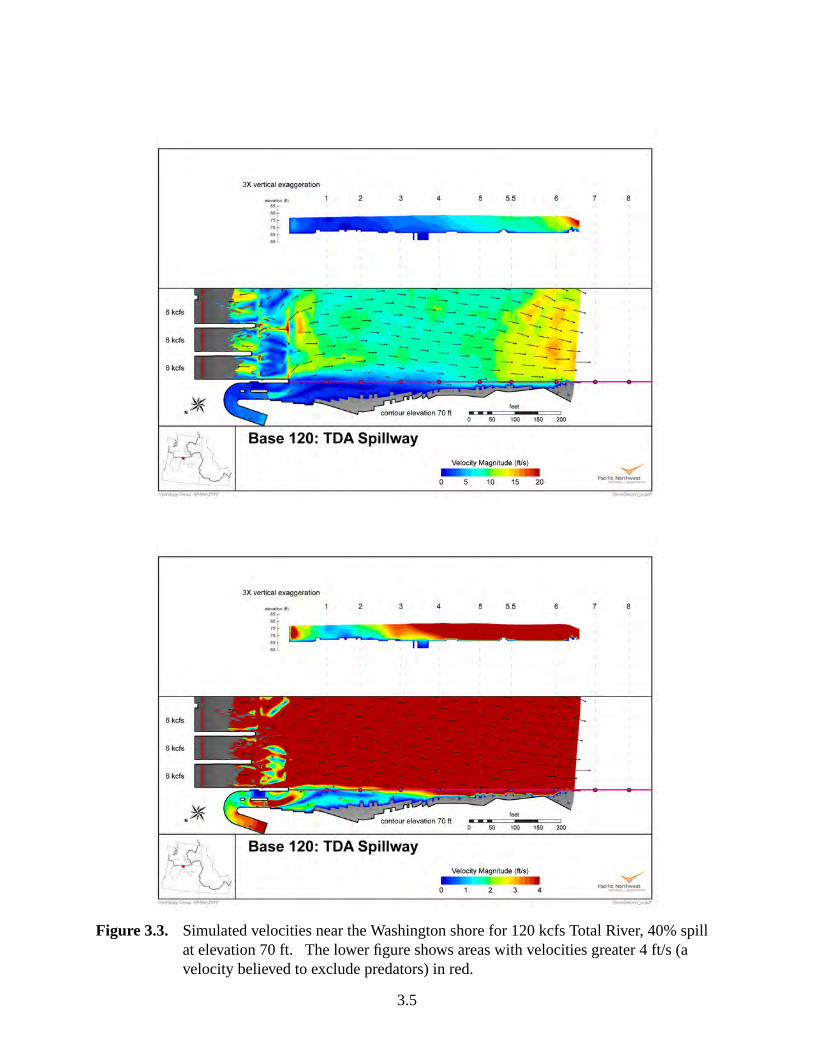
Figure 3.3. Simulated velocities near the Washington shore for 120 kcfs Total River, 40% spillat elevation 70 ft. The lower figure shows areas with velocities greater 4 ft/s (avelocity believed to exclude predators) in red.
3.5

Figure 3.4. Simulation results between the spillwall and the Washington shore for 180 kcfsTotal River, 40% spill at elevation 70 ft. The upper figure shows velocities at anelevation of 70 ft. The lower figure shows streamlines, colored by elevation, forparticles seeded downstream of the stilling basin.
3.6

Figure 3.5. Simulated velocities near the Washington shore for 180 kcfs Total River, 40% spillat elevation 70 ft. The lower figure shows areas with velocities greater 4 ft/s (avelocity believed to exclude predators) in red.
3.7

Figure 3.6. Simulation results between the spillwall and the Washington shore for 240 kcfsTotal River, 40% spill. The upper figure shows velocities at an elevation of 70ft. The lower figure shows streamlines, colored by elevation, for particles seededdownstream of the stilling basin.
3.8
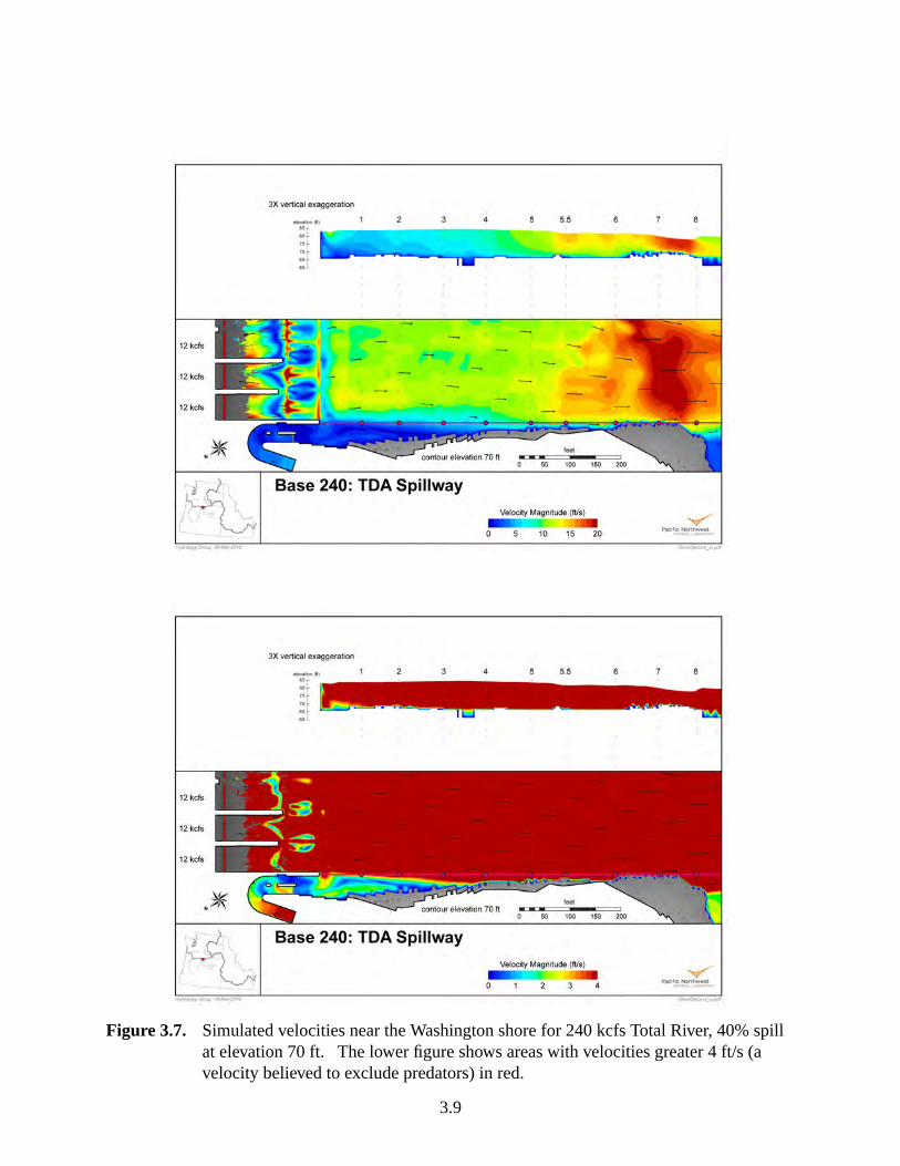
Figure 3.7. Simulated velocities near the Washington shore for 240 kcfs Total River, 40% spillat elevation 70 ft. The lower figure shows areas with velocities greater 4 ft/s (avelocity believed to exclude predators) in red.
3.9
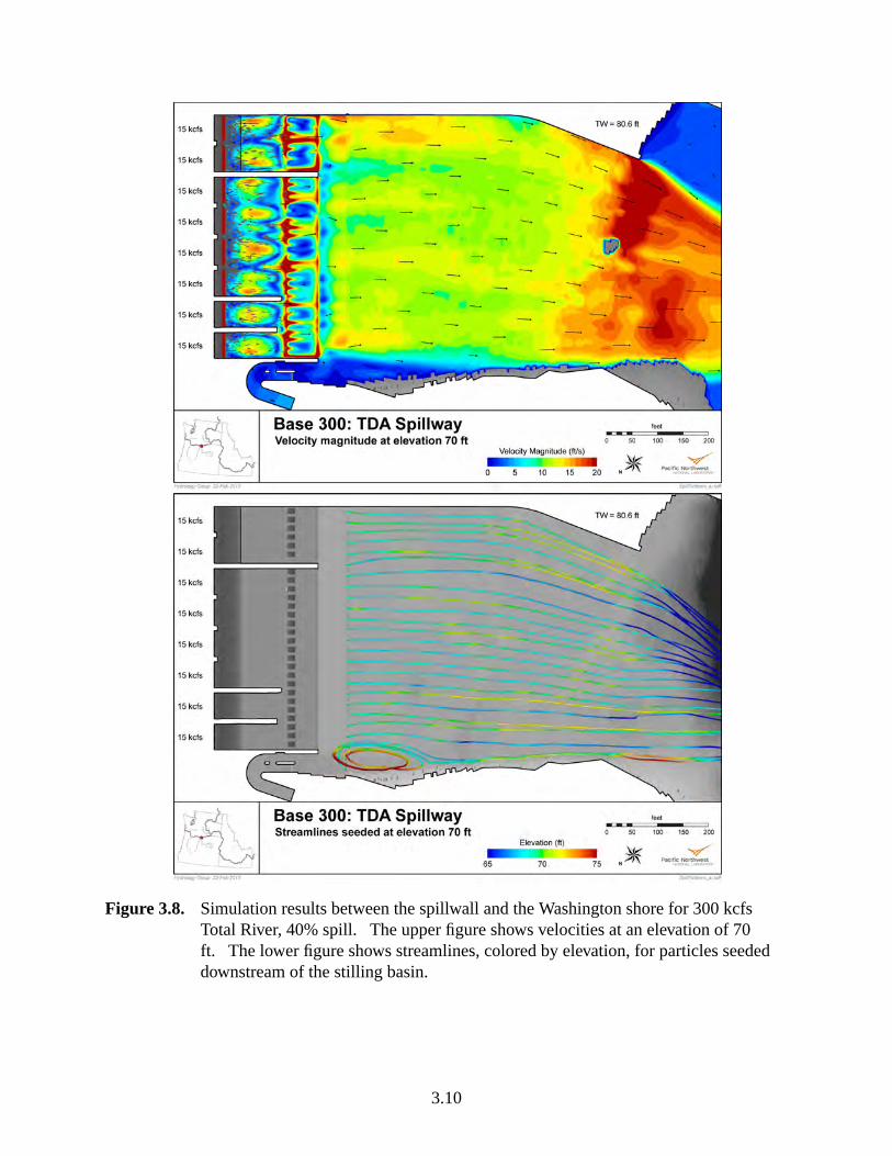
Figure 3.8. Simulation results between the spillwall and the Washington shore for 300 kcfsTotal River, 40% spill. The upper figure shows velocities at an elevation of 70ft. The lower figure shows streamlines, colored by elevation, for particles seededdownstream of the stilling basin.
3.10

Figure 3.9. Simulated velocities near the Washington shore for 300 kcfs Total River, 40% spillat elevation 70 ft. The lower figure shows areas with velocities greater 4 ft/s (avelocity believed to exclude predators) in red.
3.11

Figure 3.10. Simulation results between the spillwall and the Washington shore for 420 kcfsTotal River, 40% spill. The upper figure shows velocities at an elevation of 70ft. The lower figure shows streamlines, colored by elevation, for particles seededdownstream of the stilling basin.
3.12

Figure 3.11. Simulated velocities near the Washington shore for 420 kcfs Total River, 40% spillat elevation 70 ft. The lower figure shows areas with velocities greater 4 ft/s (avelocity believed to exclude predators) in red.
3.13

Figure 3.12. Simulation results between the spillwall and the Washington shore for 90 kcfsTotal River, 40% spill (Bays 1-6 at 6 kcfs). The upper figure shows velocities atan elevation of 70 ft. The lower figure shows streamlines, colored by elevation,for particles seeded downstream of the stilling basin.
3.14

Figure 3.13. Simulated velocities near the Washington shore for 90 kcfs Total River 40% spill(Bays 1-6 at 6 kcfs), at elevation 70 ft. The lower figure shows areas with veloci-ties greater 4 ft/s (a velocity believed to exclude predators) in red.
3.15

Figure 3.14. Simulation results between the spillwall and the Washington shore for 90 kcfsTotal River, 40% spill (Bays 3-8 at 6 kcfs). The upper figure shows velocities atan elevation of 70 ft. The lower figure shows streamlines, colored by elevation,for particles seeded downstream of the stilling basin.
3.16

Figure 3.15. Simulated velocities near the Washington shore for 90 kcfs Total River 40% spill(Bays 3-8 at 6 kcfs), at elevation 70 ft. The lower figure shows areas with veloci-ties greater 4 ft/s (a velocity believed to exclude predators) in red.
3.17

Figure 3.16. Simulation results between near the Washington shore for 90 kcfs Total River,40% spill (Bays 7 and 8 at 18 kcfs), at elevation 70 ft. The lower figure showsstreamlines, colored by elevation, seeded outside the stilling basin.
3.18
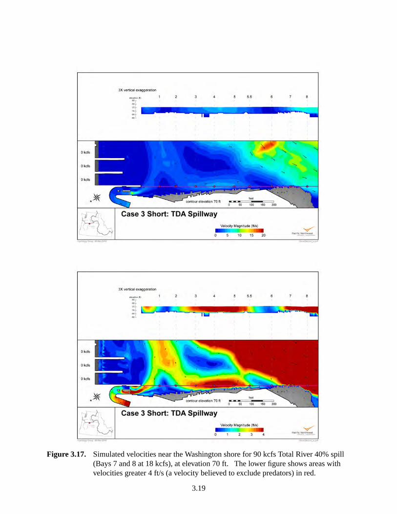
Figure 3.17. Simulated velocities near the Washington shore for 90 kcfs Total River 40% spill(Bays 7 and 8 at 18 kcfs), at elevation 70 ft. The lower figure shows areas withvelocities greater 4 ft/s (a velocity believed to exclude predators) in red.
3.19


4.0 Conclusions
This study used a CFD model to characterize tailrace hydraulics between the new spillwall andthe Washington shore for six different total river flows. The effect of spillway flow distributionwas simulated for three spill patterns at the lowest total river flow.
The model results were used in two ways. First, results graphics were provided to CENWP andregional fisheries agency representatives for use and comparison to the same flow conditions atthe ERDC reduced-scale physical model. The results graphics were very similar in flow patternto that produced by the reduced-scale physical model but these graphics provided a quantitativeview of velocity distribution. During the physical model work, an additional spill pattern wastested. Subsequently, that spill pattern was simulated in the numerical model.
The streamlines showed that the hydraulic conditions were beneficial to egress at the higher totalriver flows (120 kcfs and greater, uniform flow distribution). At the lowest flow case, 90 kcfs,it was necessary to use a non-uniform distribution. Of the three distributions tested, splittingthe flow evenly between Bay 7 and Bay 8 was deemed most beneficial for egress by CENWPfisheries biologists and regional fishery agency representatives. The numerical and physicalmodel results were very similar, building confidence in both hydraulic tools.
4.1


5.0 References
CD-adapco, Computational Dynamics Limited. 2009.CCM User Guide, STAR-CD Version4.08. CD-adapco, http://www.cd-adapco.com.
Rakowski C, W Perkins, M Richmond, and J Serkowski. 2008.Simulation of The DallesDam Proposed Full Length Spillwall. PNNL-17322, Pacific Northwest National Laboratory.Memorandum for Record to the U.S. Army Corps of Engineers Portland, Oregon.
5.1


Appendix A
Additional Graphics


Appendix A – Additional Graphics
The iso-velocity plots (Figures A.1 to A.6) are included here for completeness. These show thatthe downstream constriction of the spillwall is sufficient to create velocities that are sufficient toexclude predators from this zone for all but one case. For the 90 kcfs Case 3 with flows in Bays7 and 8 (Figure A.6), there was a narrow band near the shore with modeled velocities less that 4ft/s. However, much of the reason for doing this spill pattern was to reduce the velocities alongthe Washington shore to improve access to the North fish ladder by returning adult salmon.
A.1

Figure A.1. Iso-velocity surface for a velocity of 4 ft/s for lower flows. The upper figureshows 120 kcfs Total River. The lower figure shows 180 kcfs Total River.
A.2

Figure A.2. Iso-velocity surface for a velocity of 4 ft/s for higher flows. The upper figureshows 300 kcfs Total River. The lower figure shows 420 kcfs Total River.
A.3

Figure A.3. Iso-velocity surface for a velocity of 12 and 16 ft/s for 420 kcfs Total River.
A.4

Figure A.4. Iso-velocity surface for a velocity of 20 ft/s for 420 kcf Total Rivers.
A.5

Figure A.5. Iso-velocity surface for a velocity of 4 ft/s for 90 kcfs Total River for Cases 1 and2. The upper figure shows spill flows in Bays 1 to 6. The lower figure shows spillflows in Bays 3 to 8.
A.6

Figure A.6. Iso-velocity surface for a velocity of 4 ft/s for 90 kcfs Total River for Case 3 withspill flow in Bays 7 and 8.
A.7


