Computational Fluid Dynamics Analysis of Flexible Duct Junction Box Design Robert Beach and Duncan Prahl IBACOS, Inc.

Rich Lange Applied Science Consultants, LLC

December 2013

NOTICE

This report was prepared as an account of work sponsored by an agency of the United States government. Neither the United States government nor any agency thereof, nor any of their employees, subcontractors, or affiliated partners makes any warranty, express or implied, or assumes any legal liability or responsibility for the accuracy, completeness, or usefulness of any information, apparatus, product, or process disclosed, or represents that its use would not infringe privately owned rights. Reference herein to any specific commercial product, process, or service by trade name, trademark, manufacturer, or otherwise does not necessarily constitute or imply its endorsement, recommendation, or favoring by the United States government or any agency thereof. The views and opinions of authors expressed herein do not necessarily state or reflect those of the United States government or any agency thereof.

Available electronically at http://www.osti.gov/bridge

Available for a processing fee to U.S. Department of Energy and its contractors, in paper, from:

U.S. Department of Energy Office of Scientific and Technical Information

P.O. Box 62 Oak Ridge, TN 37831-0062

phone: 865.576.8401 fax: 865.576.5728

email: mailto:reports@adonis.osti.gov

Available for sale to the public, in paper, from: U.S. Department of Commerce

National Technical Information Service 5285 Port Royal Road Springfield, VA 22161 phone: 800.553.6847

fax: 703.605.6900 email: orders@ntis.fedworld.gov

online ordering: http://www.ntis.gov/ordering.htm

Printed on paper containing at least 50% wastepaper, including 20% postconsumer waste

iii

Computational Fluid Dynamics Analysis of Flexible Duct Junction Box Design

Prepared for:

The National Renewable Energy Laboratory

On behalf of the U.S. Department of Energy’s Building America Program

Office of Energy Efficiency and Renewable Energy

15013 Denver West Parkway

Golden, CO 80401

NREL Contract No. DE-AC36-08GO28308

Prepared by:

Robert Beach and Duncan Prahl

IBACOS, Inc.

2214 Liberty Avenue

Pittsburgh, PA 15222

Rich Lange

Applied Science Consultants, LLC

615 Washington Road, Suite 505

Pittsburgh, PA 15228

NREL Technical Monitor: Michael Gestwick

Prepared under Subcontract No. KNDJ-0-40341-03

December 2013

iv

[This page left blank]

v

Contents List of Figures ........................................................................................................................................... vii List of Tables ............................................................................................................................................ viii Definitions ................................................................................................................................................... ix Executive Summary .................................................................................................................................... x 1 Introduction and Background ............................................................................................................. 1

1.1 Introduction ..........................................................................................................................1 1.2 Background ..........................................................................................................................1

1.2.1 Existing Standards for Junction Box Design ...........................................................1 1.2.2 ASHRAE and ACCA Recommendations ................................................................4 1.2.3 Low-Load Homes, Box-Plenums, and Small-Diameter Ducts ................................5 1.2.4 Computational Fluid Dynamics and Duct Fittings ..................................................6

1.3 Research Questions ..............................................................................................................7 2 Mathematical and Modeling Methods ................................................................................................. 8

2.1 General Approach ................................................................................................................8 2.2 Computational Fluid Dynamics Modeling...........................................................................8 2.3 Inputs ................................................................................................................................11

2.3.1 Configurations, Sets, and Cases .............................................................................11 2.3.2 Ranges ....................................................................................................................11

2.4 Calculation of Pressure Losses ..........................................................................................13 2.4.1 Losses Within the Junction Box ............................................................................14 2.4.2 Losses at Transitions: From Inlet into Box and Box into Outlet ...........................15 2.4.3 Losses Associated with the Ducts ..........................................................................15 2.4.4 Balancing Losses ...................................................................................................16

2.5 Comparison to ACCA Manual D .......................................................................................16 3 Results ................................................................................................................................................. 19

3.1 Configuration A—Four Outlets .........................................................................................19 3.1.1 Set 1: Four Outlets with an Entrance Diffuser .......................................................19 3.1.2 Set 2: Four Outlets, Equal Flows ...........................................................................21 3.1.3 Set 3: Four Outlets, Unequal Flows .......................................................................22 3.1.4 Set 4: Four Outlets, Equal Flows, High Velocities ................................................24

3.2 Configuration B—Three Outlets........................................................................................25 3.2.1 Set 5: Three Outlets, Unequal Flows, Equilateral Triangle Box ...........................26 3.2.2 Set 6: Three Outlets, Equal Flows, Isosceles Triangle Box ...................................27

3.3 Configuration C—Two Outlets..........................................................................................28 3.3.1 Set 7: Two Outlets, Unequal Flows, Equilateral Triangle Box .............................29

4 Discussion ........................................................................................................................................... 31 4.1 Configuration A—Four Outlets .........................................................................................31

4.1.1 Set 1: Four Outlets with an Entrance Diffuser .......................................................31 4.1.2 Set 2: Four Outlets, Equal Flows ...........................................................................31 4.1.3 Set 3: Four Outlets, Unequal Flows .......................................................................32 4.1.4 Set 4: Four Outlets, Equal Flows, High Velocities ................................................32

4.2 Configuration B—Three Outlets........................................................................................33 4.2.1 Set 5: Three Outlets, Unequal Flows, Equilateral Triangle Box ...........................33 4.2.2 Set 6: Three Outlets, Equal Flows, Isosceles Triangle Box ...................................33

4.3 Configuration C—Two Outlets..........................................................................................33 4.3.1 Set 7: Two Outlets, Unequal Flows, Equilateral Triangle Box .............................33

vi

5 Conclusions ........................................................................................................................................ 34 5.1 How Can Current Junction Box Design Standards Be Augmented? .................................34 5.2 How Do Individual Geometric Parameters Affect the Proportions and Losses of

Airflow in Rectilinear and Triangular Junction Boxes Serving Two to Four Discrete Rooms? ..............................................................................................................................34

5.3 How Conservative Are Current ACCA Manual D, Appendix 3, Group 11 Guidelines for Designing Flexible Duct Junction Boxes? ..................................................................36

5.4 How Do Junction Boxes Perform When Outlet Duct Diameters Correspond to the Lower Room Loads of High Performance Homes? ...........................................................36

5.5 Future Research .................................................................................................................37 References ................................................................................................................................................. 38 Appendix A: Detailed Results .................................................................................................................. 39 Appendix B: Code Barriers on the Use of Flammable Materials in Space Conditioning Systems,

by Duncan Prahl ................................................................................................................................. 53

vii

List of Figures Figure 1. Typical junction box installation and assumed branch diameters (in inches) ..................... 1 Figure 2. Experimental plenum configuration and swirl phenomena ................................................... 2 Figure 3. Detail of entrance section .......................................................................................................... 3 Figure 4. Current ACCA recommended construction of flexible duct junction boxes ........................ 5 Figure 5. Schematic modular system ....................................................................................................... 6 Figure 6. Validation test configuration ..................................................................................................... 8 Figure 7. Typical mesh densities ............................................................................................................. 10 Figure 8. Configurations A, B, and C as number of outlets and box shape ....................................... 11 Figure 9. Plan and section elevation of a typical system ..................................................................... 14 Figure 10. Midplane total pressure gradient .......................................................................................... 14 Figure 11. Two entrance diffuser designs .............................................................................................. 19 Figure 12. Box and duct geometry to evaluate four outlets with an entrance diffuser ..................... 20 Figure 13. Midplane pressure gradients for four outlets with an entrance diffuser .......................... 20 Figure 14. Box and duct geometry to evaluate four outlets, equal flows ........................................... 21 Figure 15. Midplane pressure gradients for four outlets, equal flows ................................................ 22 Figure 16. Box and duct geometry to evaluate four outlets, unequal flows ....................................... 23 Figure 17. Midplane pressure gradients for four outlets, unequal flows ............................................ 24 Figure 18. Box and duct geometry to evaluate four outlets, equal flows, high velocities ................ 24 Figure 19. Midplane velocity gradients ................................................................................................... 25 Figure 20. Box and duct geometry to evaluate three outlets, unequal flows, equilateral triangle

box ....................................................................................................................................................... 26 Figure 21. Midplane pressure gradients for three outlets, unequal flows, equilateral triangle

box ....................................................................................................................................................... 27 Figure 22. Box and duct geometry to evaluate three outlets, equal flows, isosceles triangle

box ....................................................................................................................................................... 27 Figure 23. Midplane pressure gradients, three outlets, equal flows, isosceles triangle box ............ 28 Figure 24. Box and duct geometry to evaluate two outlets, unequal flows, equilateral triangle

box ....................................................................................................................................................... 29 Figure 25. Midplane pressure gradient for two outlets, unequal flows, equilateral triangle box ..... 30 Figure 26. Rectangular box ...................................................................................................................... 35 Figure 27. Triangular box, three outlets ................................................................................................. 35 Figure 28. Triangular box, two airflows .................................................................................................. 36

Unless otherwise noted, all figures and photos were created by IBACOS.

viii

List of Tables Table 1. Flow Rates for Small Duct Diameters ......................................................................................... 6 Table 2. Mesh Grid Densities ..................................................................................................................... 9 Table 3. Normalized Mass Flow Rates ...................................................................................................... 9 Table 4. Outline of Configurations Studied ............................................................................................ 13 Table 5. Four Outlets with an Entrance Diffuser, Results Summary ................................................... 21 Table 6. Four Outlets, Equal Flows, Results Summary ......................................................................... 22 Table 7. Four Outlets, Unequal Flows, Results Summary .................................................................... 23 Table 8. Four Outlets, Equal Flows, High Velocities, Results Summary. ............................................ 25 Table 9. Three Outlets, Unequal Flows, Equilateral Triangle Box, Results Summary ....................... 26 Table 10. Three Outlets, Equal Flows, Isosceles Triangle Box, Results Summary............................ 28 Table 11. Two Outlets, Unequal Flows, Equilateral Triangle Box, Results Summary........................ 29 Table 12. Set 1: Four and Five Outlets with an Entrance Diffuser, Fully Developed Losses ............ 39 Table 13. Set 1: Four and Five Outlets with an Entrance Diffuser, Detailed Results ......................... 40 Table 14. Set 2: Four Outlets, Equal Flows, Fully Developed Losses ................................................. 41 Table 15. Set 2: Four Outlets, Equal Flows, Detailed Results .............................................................. 42 Table 16. Set 3: Four Outlets, Unequal Flows, Fully Developed Losses ............................................. 43 Table 17. Set 3: Four Outlets, Unequal Flows, Detailed Results .......................................................... 44 Table 18. Set 4: Four Outlets, Equal Flows, High Velocities, Fully Developed Losses ..................... 45 Table 19. Set 4: Four Outlets, Equal Flows, High Velocities, Detailed Results .................................. 46 Table 20. Set 5: Three Outlets, Unequal Flows, Equilateral Triangle Box, Fully Developed

Losses ................................................................................................................................................. 47 Table 21. Set 5: Three Outlets, Unequal Flows, Equilateral Triangle Box, Detailed Results ............ 48 Table 22. Set 6: Three Outlets, Equal Flows, Isosceles Triangle Box, Fully Developed Losses ...... 49 Table 23. Set 6: Three Outlets, Equal Flows, Isosceles Triangle Box, Detailed Results ................... 50 Table 24. Set 7: Two Outlets, Unequal Flows, Equilateral Triangle Box, Fully Developed Losses .. 51 Table 25. Set 7: Two Outlets, Unequal Flows, Equilateral Triangle Box, Detailed Results ............... 52 Table 26. Approximate Flow Rates for Duct Diameters ........................................................................ 54 Table 27. Flame Spread and Smoke Developed Ratings From the 2012 IRC ..................................... 56 Table 28. Flame Spread and Smoke Developed of Common Materials ............................................... 56 Table 29. Requirements in Various Sections of the 2012 IRC to Limit Loss of Life and Fire

Promulgation ....................................................................................................................................... 57

Unless otherwise noted, all tables were created by IBACOS.

ix

Definitions

ACCA Air Conditioning Contractors of America

ACCA Manual D Air Conditioning Contractors of America Manual D

Btuh British thermal units per hour

CFD Computational fluid dynamics

cfm Cubic feet per minute

DOE U.S. Department of Energy

EL Equivalent length

HVAC Heating, ventilation, and air conditioning

IECC International Energy Conservation Code

IRC International Residential Code

IWC Inches of water column

NBFU National Board of Fire Underwriters

x

Executive Summary

This research explores the relationships between pressure and physical configurations of flexible duct junction boxes. Through a suite of computational fluid dynamics (CFD) simulations, relationships between individual box parameters and total system pressure have been predicted.

The current Air Conditioning Contractors of America (ACCA) guidance found in Group 11 of Appendix 3 in ACCA Manual D (Rutkowski 2009) allows for unconstrained variation in the number of takeoffs, box sizes, and takeoff locations. The only variables currently used in selecting an equivalent length (EL) are the velocity of the air in the duct and the friction rate, given the first takeoff is located at least twice its diameter away from the inlet. This condition does not account for other factors having an impact on pressure loss across these types of fittings.

Due to this loosely constrained model for box design, contractors are using the fitting as a low-cost, “one-size-fits-all” solution and are circumventing the principle of right-sizing heating, ventilation, and air conditioning (HVAC) systems. Rather than completely eliminating the fitting—cost and flexibility are necessary considerations when choosing components—IBACOS believes better guidance can improve the performance of duct systems using this fitting.

To analyze the individual effects of the acting parameters, the IBACOS team used a series of CFD simulations to quantify the effects of different box designs. Appendix A documents the detailed simulation inputs and results. For each simulation, the team converted the pressure loss within the box to an EL to compare the variation in the ACCA Manual D guidance to the simulated variation. IBACOS chose cases that correlate reasonably to flows typically encountered in the field as determined by a survey of ACCA Manual J (Rutkowski 2006) load calculations of typical house plans from across the country. The team analyzed differences in total pressure due to increases in the number and location of takeoffs, the box dimensions, the velocity of the air (currently the only parameter accounted for with ACCA Manual D Group 11 fittings), and whether the entrance fitting is included (currently optional). Furthermore, and perhaps most important, the team calculated the additional balancing losses for all cases due to discrepancies between the intended outlet flows and the natural flow splits created by the fitting.

IBACOS developed general recommendations intended to supplement current guidance. Most importantly, this report reiterates the need for balancing dampers on all duct runs. ACCA Manual D predicates its entire design process on this condition. The outlet flows of a specific junction box are highly sensitive to its geometry, and it is unrealistic to build a box that will predictably divide the airflow into target rates. Also, balancing losses are significantly higher when there is an outlet directly opposite the inlet; therefore, outlets should be placed only on the sides.

An important goal for a designer is to implement symmetry in the junction box wherever possible. In certain asymmetrical cases, balancing losses were found to be significantly higher than in other symmetrical cases where the unbalanced splits were reasonably close to the targets.

Junction box size is another important factor to consider. To conserve material, junction boxes should be made as small as possible. However, outlets should be placed at the rear of the

xi

junction box to minimize pressure losses. Likewise, junction box width will help to minimize oscillations and instabilities in the airflow. The research team proposes to limit the allowable number of takeoffs to three and four; a trunk and branch system is far more efficient when more than four takeoffs are needed, and a metal wye fitting is better when splitting only in two.

In parallel with this technical report, IBACOS is developing a related Measure Guideline that will document a constrained approach to designing junction boxes that utilizes the trends observed in these simulations.

1

1 Introduction and Background

1.1 Introduction Currently, the production home-building industry prefers junction boxes as the primary means to split airflow in flexible duct HVAC systems. This is largely due to the flexibility of design, compact size, and low cost of junction boxes. However, implementation in the field is substandard, characterized by poorly performing HVAC systems and occupant complaints.

ACCA Manual D outlines the standard procedure for designing residential duct systems. However, the “recommended” geometric parameters of the boxes do not account for all factors affecting the pressure drop across a balanced junction box and therefore offer no guarantee to the designer that the EL values are accurate. Better guidance is needed for right-sized duct system design.

Although low in cost, junction boxes are poorly implemented by trades in production environments. Figure 1 depicts a common installation configuration. Although the flexible duct installation shown in this figure is good (i.e., well supported, smooth radius turns, duct pulled to full length), the junction box does not adhere to ACCA design parameters, and no dampers are installed to balance the flow after installation. This box probably does not perform as intended by the HVAC designer.

Figure 1. Typical junction box installation and assumed branch diameters (in inches)

1.2 Background 1.2.1 Existing Standards for Junction Box Design All existing standards relating to the design of junction boxes to pressure loss apparently follow from experiments done by Gilman et al. (1951). Their study was “a laboratory investigation of the pressure characteristics and air distribution in a type of plenum chamber designated as a box-plenum.” Their research found that rotational flow in the plenum could occur with a number of different entrance conditions and that the rotational flow could change direction, resulting in

What is WUFI?

166

6

6

6

68

8

8

24x24x40 Box

Assumed sizes

2

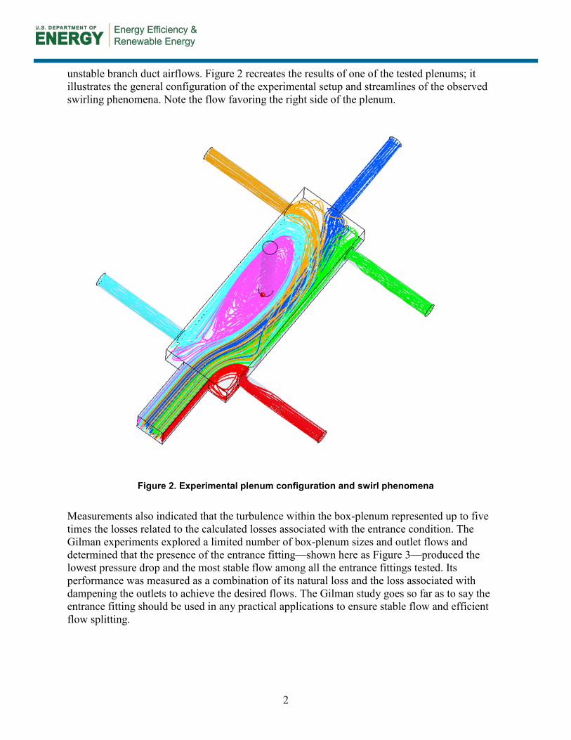
unstable branch duct airflows. Figure 2 recreates the results of one of the tested plenums; it illustrates the general configuration of the experimental setup and streamlines of the observed swirling phenomena. Note the flow favoring the right side of the plenum.

Figure 2. Experimental plenum configuration and swirl phenomena

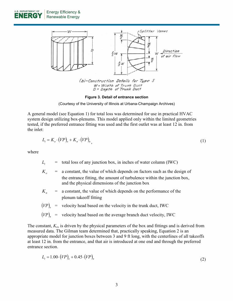
Measurements also indicated that the turbulence within the box-plenum represented up to five times the losses related to the calculated losses associated with the entrance condition. The Gilman experiments explored a limited number of box-plenum sizes and outlet flows and determined that the presence of the entrance fitting—shown here as Figure 3—produced the lowest pressure drop and the most stable flow among all the entrance fittings tested. Its performance was measured as a combination of its natural loss and the loss associated with dampening the outlets to achieve the desired flows. The Gilman study goes so far as to say the entrance fitting should be used in any practical applications to ensure stable flow and efficient flow splitting.

3

Figure 3. Detail of entrance section

(Courtesy of the University of Illinois at Urbana-Champaign Archives) A general model (see Equation 1) for total loss was determined for use in practical HVAC system design utilizing box-plenums. This model applied only within the limited geometries tested, if the preferred entrance fitting was used and the first outlet was at least 12 in. from the inlet:

( ) ( )nnoot VPKVPKL ⋅+⋅= , (1)

where

tL = total loss of any junction box, in inches of water column (IWC)

oK = a constant, the value of which depends on factors such as the design of the entrance fitting, the amount of turbulence within the junction box, and the physical dimensions of the junction box

nK = a constant, the value of which depends on the performance of the plenum takeoff fitting

( )oVP = velocity head based on the velocity in the trunk duct, IWC

( )nVP = velocity head based on the average branch duct velocity, IWC

The constant, Ko, is driven by the physical parameters of the box and fittings and is derived from measured data. The Gilman team determined that, practically speaking, Equation 2 is an appropriate model for junction boxes between 3 and 9 ft long, with the centerlines of all takeoffs at least 12 in. from the entrance, and that air is introduced at one end and through the preferred entrance section.

( ) ( )not VPVPL ⋅+⋅= 45.000.1 (2)

4

Note that the model coefficients in Equation 2 are specific to the physical parameters of the box and would change if, for example, a different entrance fitting were used.

1.2.2 ASHRAE and ACCA Recommendations ASHRAE (2012) directly references the Gilman study (Gilman et al. 1951) and states that 0.05 in. of water value is appropriate to account for pressure loss through the plenum, provided a stability-inducing entrance fitting is included, the blower is moving less than 2,250 cfm, and the box proportions are limited as follows:

• The minimum clearance between the first outlet and the inlet is two-thirds times the inlet width.

• The box width is 2.5 times the entrance width.

• The length of the box is twice its width.

ACCA Manual D describes a comprehensive set of recognized duct sizing principles and calculations for optimizing the design of residential duct systems. Appendix 3 of ACCA Manual D provides information about the airflow resistance produced by various types of supply and return fittings. For residential duct systems, and as a matter of convenience, this resistance has been quantified by assigning an EL value to each type of fitting. EL values allow for the determination of the longest run, which is used to select the right-sized blower. Junction box EL values are provided in ACCA Manual D Group 11 and are assumed to be valid if the box construction adheres to the following recommendations and the accompanying diagram shown here as Figure 4 (Rutkowski 2009):

1. “The entrance has a diffuser fitting that recovers velocity pressures and prevents swirl (optional).

2. There should be a straight approach and straight exits.

3. Exit openings are on only the side (no top or bottom exits).

4. There should be an exit opening at least two diameters from the entrance: DL ×= 2 .

5. Make the box as small as possible, but comply with rule 4.”

Equivalent length: For duct fittings, the airflow resistance produced by a fitting is equivalent to the quantity of feet of straight duct that produces the same airflow resistance (Rutkowski 2009).

5

Figure 4. Current ACCA recommended construction of flexible duct junction boxes

(Rutkowski 2009) 1.2.3 Low-Load Homes, Box-Plenums, and Small-Diameter Ducts Codes for new construction have significantly improved, and houses built to the 2012 International Energy Conservation Code (IECC 2012) can have load densities of 900–1,200 ft2/12,000 Btu/h of nominal cooling. This translates to roughly 0.33–0.44 cfm of conditioned air/ft2 of living area at peak conditions. This leads to bedroom airflows of 40–100 cfm and aggregate living space airflows of 150–250 cfm. Appendix B includes more technical details relating to this topic.

These realities of new construction also are finding their way into existing homes that are undertaking moderate to deep energy retrofits. Although the load densities in these existing homes are somewhat lower, the problem remains for downsized air handling equipment being installed in oversized leaky ducts in attics. Likewise, it is difficult to retrofit a duct system below the conditioned ceiling, with the associated loss of floor space for the air handler and extensive soffits needed to accommodate ducts from a central HVAC unit.

Research by Ridouane and Gawlik (2011) has shown that high sidewall interior supply registers can provide good comfort for occupants. Ridouane (2010) shows that 500 and 700 fpm for heating and cooling, respectively, provide enough momentum for air to mix in the room and that lower temperature air at the outlets in heating mode is desirable to minimize stratification.

Residential space conditioning equipment typically consists of one unit for the entire house. Historically, high-end systems were split into two systems to zone the house but still relied on a central air handler with a duct system that distributes the air throughout the zone. Proper design of duct systems becomes increasingly difficult as the room airflow requirements drop, especially when attempting to keep the system in reasonable balance and with higher air velocity supply outlets to facilitate mixing in the room.

One solution to this problem is not to use a central heating and cooling unit with ducts running throughout the house. If the heating and cooling system (air handling units and associated ductwork) is broken down into smaller discrete parts, multiple systems can serve different spaces. Locating systems in close proximity to the loads served enables significantly shorter duct

6

runs, lower static pressures in the system, and potentially greater use of temperature setup/setback in unoccupied spaces (e.g., bedrooms).

To make this strategy feasible in the United States, two major hurdles must be overcome. The first challenge is the availability and cost of equipment, which is less of a technical challenge and more of a market challenge. The other factor is low-cost, simple, leak-free duct systems that can be modularized to accommodate the necessary airflows for each room in increments of approximately 10–15 cfm. Table 1 gives approximate flow rates for various duct diameters.

Table 1. Flow Rates for Small Duct Diameters

Duct Diameter, in.

cfm @ 500 fpm

cfm @ 700 fpm

1.5 6 9 2 11 15 3 25 34 4 44 61 5 68 95 6 98 137

Small modular systems (small fan coil units), as shown schematically in Figure 5, will have configurations similar to those shown in ACCA Manual D, Group 11 of Appendix 3.

Figure 5. Schematic modular system

1.2.4 Computational Fluid Dynamics and Duct Fittings Contemporary research is looking into methods for producing pressure drop data for HVAC designers without the need for physical testing. This effort is driven by the high costs associated with physical testing, and CFD is viewed as one possible solution that can provide rapid

7

turnaround for new duct fittings without the need for physical testing of every configuration (Shao and Riffat 1995).

Shao and Riffat (1995) detailed the factors when using CFD that affect the accuracy of pressure loss estimations in duct fittings. They analyzed the effects of grid density and distribution, choice of turbulence models, interpolation schemes, and the length of downstream ducts. They determined that, for any dissimilar fitting, CFD simulation parameters should be calibrated to experimental data.

Mumma et al. (1998) performed a series of CFD simulations and parallel experiments, concluding that CFD could effectively determine ductwork loss coefficients. However, in very low loss cases, the simulations disagreed with the experimental data, which could be attributed to incorrect surface roughness.

Liu et al. (2012) submitted an entry to a competition for determining pressure loss coefficients for duct fittings with no experimental data against which to calibrate, organized by the ASHRAE Technical Committee on Duct Design. Mesh sizes of about 10 mm were sufficient to minimize grid density–induced errors. Pressure loss was determined to be highly sensitive to surface roughness used to calculate friction factors. The standard k-ε (k-epsilon) turbulence model was employed, and the estimated pressure drop matched the measured data well. Generally, the CFD predictions were within 20% of the measured data.

1.3 Research Questions Based on this past work and the anticipated continuation of the use of the junction box, IBACOS believes certain configurations will minimize the EL and simplify the required balancing necessary to achieve specific flow rates. Conversely, there are likely times when a junction box should not be used. This project seeks to characterize the junction box geometric configurations and location of ducts in those boxes that optimize the EL and need very little balancing.

The following research questions were asked as part of this project:

• How can current junction box design standards be augmented?

• How do individual geometric parameters affect the proportions and losses of airflow in rectilinear and triangular junction boxes serving two to four discrete rooms?

• How conservative are current ACCA Manual D, Appendix 3, Group 11 guidelines for designing flexible duct junction boxes?

• How do junction boxes perform when outlet duct diameters correspond to the lower room loads of high performance homes?

8

2 Mathematical and Modeling Methods

2.1 General Approach IBACOS used the background research to inform the construction of three-dimensional CFD models that represent a small subset of possible junction box configurations. The team used these models to analyze various parameters over which a designer would have control. The team calibrated the CFD model against the limited experimental data and the calculation methods documented in the background research.

2.2 Computational Fluid Dynamics Modeling Figure 6 illustrates a configuration replicated from the Gilman study for which there was documentation of the measurements. Outlet numbers are noted. The measurements were used to validate the simulation parameters and appropriate mesh grid densities. Although not a rigorous validation, the results confirm the simulations are realistic. All outlets in this configuration are 7 in. The box dimensions are 3 ft × 3 ft and 1 ft tall.

Figure 6. Validation test configuration

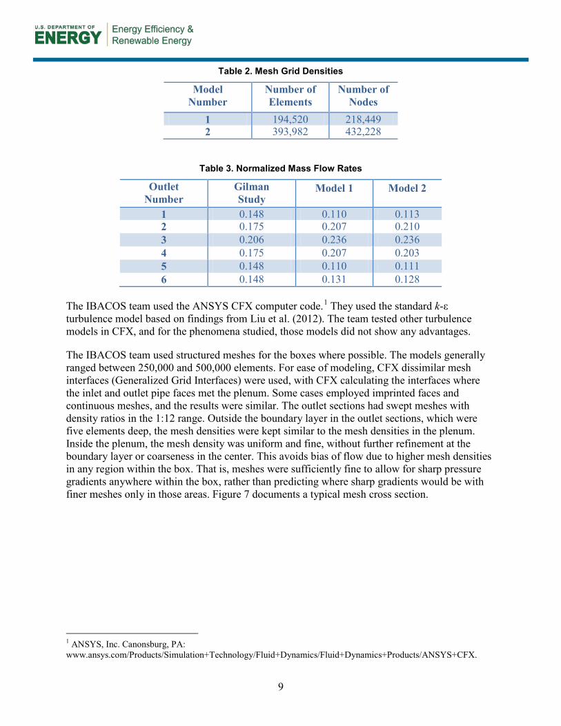
Table 2 shows the mesh grid densities of Model 1 and Model 2. Table 3 documents the data taken from the Gilman study and the corresponding results of two grid densities. The density roughly doubled between the two, yet there was very little change between the normalized mass flow rates. Therefore, meshes in subsequent cases used grid densities within the Table 2 range. There is qualitative agreement between the Gilman study and the simulation presented here, but rigorous calibration was not done because of uncertainties in the Gilman measurements.

1

2

5

4

6

3

9

Table 2. Mesh Grid Densities

Model Number

Number of Elements

Number of Nodes

1 194,520 218,449 2 393,982 432,228

Table 3. Normalized Mass Flow Rates

Outlet Number

Gilman Study

Model 1 Model 2

1 0.148 0.110 0.113 2 0.175 0.207 0.210 3 0.206 0.236 0.236 4 0.175 0.207 0.203 5 0.148 0.110 0.111 6 0.148 0.131 0.128

The IBACOS team used the ANSYS CFX computer code.1 They used the standard k-ε turbulence model based on findings from Liu et al. (2012). The team tested other turbulence models in CFX, and for the phenomena studied, those models did not show any advantages.

The IBACOS team used structured meshes for the boxes where possible. The models generally ranged between 250,000 and 500,000 elements. For ease of modeling, CFX dissimilar mesh interfaces (Generalized Grid Interfaces) were used, with CFX calculating the interfaces where the inlet and outlet pipe faces met the plenum. Some cases employed imprinted faces and continuous meshes, and the results were similar. The outlet sections had swept meshes with density ratios in the 1:12 range. Outside the boundary layer in the outlet sections, which were five elements deep, the mesh densities were kept similar to the mesh densities in the plenum. Inside the plenum, the mesh density was uniform and fine, without further refinement at the boundary layer or coarseness in the center. This avoids bias of flow due to higher mesh densities in any region within the box. That is, meshes were sufficiently fine to allow for sharp pressure gradients anywhere within the box, rather than predicting where sharp gradients would be with finer meshes only in those areas. Figure 7 documents a typical mesh cross section.

1 ANSYS, Inc. Canonsburg, PA: www.ansys.com/Products/Simulation+Technology/Fluid+Dynamics/Fluid+Dynamics+Products/ANSYS+CFX.

10

Figure 7. Typical mesh densities

The research team applied turbulent, fully developed velocity profiles calculated by CFX to the inlet pipe entrances. They did not simulate cases where a bend occurred near the entrance to the box. Outlet ducts were sufficiently long—in most cases, 200 in.—to allow the flow to fully develop after exiting the box.

The mass fractions exiting each of the modeled outlets were tracked with monitor points. Some models were stable, with mass and momentum residuals as defined by CFX achieving levels as low as 1.E-6. Some cases were oscillatory in nature, and once a repeatable pattern of monitor point oscillation was achieved, the calculations were halted at the local extremes. The team used symmetry conditions in many cases; however, because it is known that, in some cases, symmetry conditions suppress oscillations, full models also were employed.

In the outlets, surface roughnesses were applied to the duct boundaries to induce pressure losses corresponding to the implied roughness values from a duct sizing slide rule. The slide rule specifies loss rates (IWC/100 ft) for given volumetric flow rates within flex duct of specific diameters. Simulation surface roughness values were tuned until pressure drops in straight ducts precisely matched the loss rates for duct diameters specified by the slide rule.

Within the box, roughnesses were specified to match duct board material. Full calibration of the surface characteristics was not performed because the focus was on relative differences due to configurations. To precisely analyze the EL tables, surface roughnesses would need to be calibrated to measured data as discussed in the Background section.

Automatic time stepping was used. Results where flow oscillations occurred were checked by lowering the time step. The flow oscillations persisted, indicating they likely exist in real-world duct systems. The team found that some of the situations modeled had fundamental instabilities, replicating the results of Gilman’s study (Gilman et al. 1951).

In some studies, flow balancing was required to make outlet flows match the design flow. When balancing was needed, small regions at the ends of the outlets were made into sub-domains with applied momentum sources terms. The resistance regions were placed sufficiently far from the box to allow the flow to fully develop in the outlets, thus isolating the effect of the added resistance. How, specifically, a physical balancing damper would add resistance was not simulated. Only the quantity of back pressure applied to achieve a balanced state was necessary for this study. In some instances, these were “k-factors”; more often, a permeability-type loss

11

was applied. The team varied the values until the target flow splits were achieved with at least one outlet with zero additional resistance.

2.3 Inputs The total number of possible variations in junction boxes is impractical to exhaustively characterize. Currently, the ACCA Manual D Group 11 fittings constrain the design and assume that the same pressure values apply for all possible configurations. ACCA provides little guidance on the millions of configurations possible based on box dimensions, number of outlets, diameters, and airflows. Additionally, designers seeking to minimize the amount of balancing and to maximize system performance are not served by ACCA Manual D.

2.3.1 Configurations, Sets, and Cases For this project, the team developed three different, general configurations and within those configurations developed sets to enable varying of different parameters. Within each set, a specific case was developed that represents a single model with all the parameters defined. A “reference case” was developed to simulate one configuration similar to that used by Gilman et al. (1951). In all, 53 individual cases were simulated for this project, documenting variations in pressure loss across a small sample of designs. A detailed description of the sets and cases can be found in Appendix A.

2.3.2 Ranges For this project, the team designed the cases to represent a reasonable range of parameters, based on field experience of what likely conditions would be across a range of airflows.

2.3.2.1 Number of Outlets IBACOS chose to bound the problem by using typical configurations seen in the field that would serve from two to four rooms in a home. Figure 8 diagrams these three configurations (Configurations A, B, and C) in terms of the number of outlets tied to a box shape. The team suspected that this limitation in itself would lead to better correlation between ACCA Manual D pressure drops and the simulations and ultimately the installed systems.

Figure 8. Configurations A, B, and C as number of outlets and box shape

2.3.2.2 Flow Rates The IBACOS team chose flow rates to represent those commonly encountered in the field. For the purposes of this study, the research team used flow rates of 10, 100, and 250 cfm as

12

commonly occurring flow rates bounding a typical range. The team chose experimental cases to contain combinations of these flows. Because most rooms with higher loads would contain at least two registers to supply the air, the maximum flow rate for the experiments was 250 cfm. For HVAC systems in high performance homes, 10 cfm is seen as a reasonable modular value. This also was a flow rate associated with ventilation, which, in low-load homes, may be the dominant requirement for sizing the ducts.

The team also studied asymmetrical cases to determine if a single EL value was appropriate when the flow split was non-uniform. Many duct fittings that have a highly asymmetrical configuration are given different EL values for the outlets, whereas junction boxes receive only one value. This hypothesis is based on ACCA Manual D fittings with this condition, such as Group 9A fittings, which are given two EL values.

2.3.2.3 Duct Sizing The IBACOS team sized ducts to the nearest nominal diameter using a flex duct calculator with the desired cfm flow rate and a design friction rate as close to, but not exceeding, 0.08 IWC (20 Pa)/100 ft of EL. The duct diameters were controlled by the flow rates due to this constraint. In one set, velocities were roughly doubled for the same duct diameters, which resulted in significantly higher pressures.

2.3.2.4 Box Dimensions, Outlet Locations, and Outlet Spacing To study the effects of box dimensions, the IBACOS team simulated a variety of sizes. Every set included the minimum-sized box based on minimum 2-in. spacing between outlets and between ducts and box edges. This encompassed what a builder would prefer, namely, material efficiency. It called into question and tested the requirement of two times the outlet diameter spacing between the inlet and the first outlet. The goal was to provide more specific insight into how box dimensions may be leveraged to achieve better performing fittings. Within reason, the team also tested larger box sizes to see if they provide an advantage (or disadvantage) in pressure loss.

2.3.2.5 Summary of Configurations and Sets Table 4 shows a general breakdown of the configurations and sets, with comments on the parameters varied for the cases and the reasons for the variations.

13

Table 4. Outline of Configurations Studied

Configuration (see Figure 8) Set Name Remarks

A 1 Four outlets with an entrance diffuser

Investigate the benefit of an entrance diffuser similar to the type 5 design presented by

Gilman et al. (1951).

A 2 Four outlets, equal flows

Box dimensions and outlet spacing were varied. Inlet flow remained constant.

A 3 Four outlets, unequal flows

Outlet locations were swapped to determine the best way to lay out outlets of different

flows. Box dimensions, flow rates, and outlet centerlines were held constant.

B 4 Four outlets, equal flows, high velocities

Three inlet cfm values and, for each of these, two outlet velocities were simulated to gauge

the effect of increased velocity. B 5 Three outlets, unequal

flows, equilateral triangle box

An asymmetrical case with two different box sizes was considered. The boxes were

equilateral triangles to achieve a wider profile. The effect of box size and outlet locations

along the sides was simulated. B 6 Three outlets, unequal

flows, isosceles triangle box

Three outlet cfm values were simulated in minimum-sized, isosceles-triangle-shaped

boxes. Locations of the outlet on the left side were varied.

C 7 Two outlets, unequal flows, equilateral

triangle box

A simple two-outlet box with unequal outlet flows was considered. Two box sizes were simulated, and the locations of the outlets

were varied. 2.4 Calculation of Pressure Losses This study simulated the pressure losses associated with a total system consisting of an inlet duct, an inlet duct to junction box connection, a triangular or rectangular junction box, a box to outlet duct connection, two to four outlet ducts, and any balancing that was necessary to achieve design airflows. The IBACOS team simulated the full system to prevent negating effects occurring outside the box confines yet due to the box’s inefficiencies in turning/splitting the flow. Figure 9 shows an example system configuration. Figure 10 shows an example resultant total pressure gradient of two cases from Set 3.

14

Figure 9. Plan and section elevation of a typical system

Figure 10. Midplane total pressure gradient

2.4.1 Losses Within the Junction Box The primary output from the simulations is a pressure loss value attributed to the junction box. For each simulated case, the team calculated the pressure loss in the box by subtracting the normal, fully developed losses associated with the outlet duct and straight inlet from the total pressure of the system measured at the inlet, as shown in Equation 3:

15

)( outletinlettotalbox PPPP ∆+∆−∆=∆ , (3)

where

boxP∆ = pressure drop attributed to the junction box

totalP∆ = total pressure drop from the beginning of the inlet to the end of the outlet

inletP∆ = pressure drop of a fully developed flow profile across the inlet’s length, from Equation 5

outletP∆ = pressure drop of a fully developed flow profile across the outlet’s length, from Equation 5

2.4.2 Losses at Transitions: From Inlet into Box and Box into Outlet The junction box as a fitting connects the two ducts together and changes the characteristics of the flow leaving the inlet duct and entering the outlet ducts. These are characterized as abrupt expansion and contraction geometries. The research team made a comparison between a veined entrance fitting and an abrupt expansion fitting, and the outlet fitting geometry was held constant throughout the experiments.

2.4.3 Losses Associated with the Ducts Taken individually, the inlet and outlet ducts have losses associated with them equal to their loss rate (IWC/unit length) times their length. Outlets were extended by the rule of thumb 10 diameters to allow for a fully developed flow to occur at the end of the outlet. This enabled the team to calculate the losses inside the outlet duct that were created by the outlet condition between the box and duct.

The relationship of the roughness values within the CFD simulations was used to calculate the friction factor in Equation 4. The Moody diagram (Moody 1944) gives the friction factor for a Reynolds number and relative roughness. The relative roughness is equal to the surface roughness (from the simulation) divided by the diameter. Equation 4 was shown to estimate the same pressure drop for a straight section of pipe as a simple CFD simulation.

The research team calculated a head loss rate (IWC/100 ft) using the Darcy–Weisbach formula shown in Equation 4:

cwater

air

hw g

VD

LfH⋅⋅⋅⋅

⋅⋅

=2

144 2

ρρ

, (4)

where

wH = head loss rate, IWC/100 ft

f = friction factor, taken from the Moody diagram

16

L = length of the duct, 100 ft

hD = hydraulic diameter of the duct, ft

airρ = constant, density of air, lb/ft3

waterρ = constant, density of water, lb/ft3

V = velocity of the air, ft/s

cg = conversion factor, 32.174 lbm ∙ ft/lbf ∙ s2

For each case, the team multiplied the head loss by the lengths of the inlet and outlet ducts to obtain the normal, fully developed losses associated with them, as shown in Equation 5. Because the simulation results were reported in Pascals, the team converted the loss in IWC to Pascals by multiplying by 248.84.

100

84.248⋅⋅=∆

LHP wduct , (5)

where

ductP∆ = inlet or outlet duct pressure drop, Pa

wH = head loss rate, IWC/100 ft

L = length of the duct, ft

2.4.4 Balancing Losses The flow splits have direct implications on the amount of balancing required. The natural flow split is equal to the ratio of the outlet’s area to the total area of all the outlets. The target flow split is the flow split determined by the designer. Balancing is needed when a design does not achieve an ideal natural split due to limitations in standard duct sizes and the layout of the fittings. In junction boxes, this design failure must be made up with additional balancing. The intent of a high performance system designer is to minimize the amount of balancing necessary to maximize efficiency.

In any given case, at least one outlet will not need additional resistance. In cases where the layout is symmetrical, more than one outlet may not need additional resistance. Balanced conditions are compared to ACCA Manual D values because given EL values assume balanced flow values. Natural flows that were within 10% of the target were deemed to be acceptable and were not further balanced because ACCA Manual D is a conservative approximation. In pre-balanced conditions, each outlet will have a different EL.

2.5 Comparison to ACCA Manual D ACCA Manual D provides EL values for duct fittings, which are used to determine the amount of pressure the blower must overcome in an HVAC system. These values are supplied with

17

reference velocities and friction rates. In ACCA Manual D Group 11 fittings, a range of outlet duct velocities is provided, with corresponding EL values for designing systems that use these fittings.

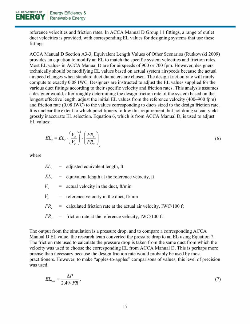
ACCA Manual D Section A3-3, Equivalent Length Values of Other Scenarios (Rutkowski 2009) provides an equation to modify an EL to match the specific system velocities and friction rates. Most EL values in ACCA Manual D are for airspeeds of 900 or 700 fpm. However, designers technically should be modifying EL values based on actual system airspeeds because the actual airspeed changes when standard duct diameters are chosen. The design friction rate will rarely compute to exactly 0.08 IWC. Designers are instructed to adjust the EL values supplied for the various duct fittings according to their specific velocity and friction rates. This analysis assumes a designer would, after roughly determining the design friction rate of the system based on the longest effective length, adjust the initial EL values from the reference velocity (400–900 fpm) and friction rate (0.08 IWC) to the values corresponding to ducts sized to the design friction rate. It is unclear the extent to which practitioners follow this requirement, but not doing so can yield grossly inaccurate EL selection. Equation 6, which is from ACCA Manual D, is used to adjust EL values:

⋅

⋅=

x

r

r

xrx FR

FRVVELEL

2

, (6)

where

xEL = adjusted equivalent length, ft

rEL = equivalent length at the reference velocity, ft

xV = actual velocity in the duct, ft/min

rV = reference velocity in the duct, ft/min

xFR = calculated friction rate at the actual air velocity, IWC/100 ft

rFR = friction rate at the reference velocity, IWC/100 ft

The output from the simulation is a pressure drop, and to compare a corresponding ACCA Manual D EL value, the research team converted the pressure drop to an EL using Equation 7. The friction rate used to calculate the pressure drop is taken from the same duct from which the velocity was used to choose the corresponding EL from ACCA Manual D. This is perhaps more precise than necessary because the design friction rate would probably be used by most practitioners. However, to make “apples-to-apples” comparisons of values, this level of precision was used.

FR

PELbox ⋅∆

=49.2

, (7)

18

where

boxEL = calculated equivalent length of the box from CFD simulation, ft

P∆ = box pressure drop, Pa

FR = friction rate, IWC/100 ft

2.49 = conversion from Pascals to IWC

19

3 Results

This section provides an overview of the simulation results, focusing on the extents of variations from each set. A diagram is supplied for each set, illustrating how cases vary within the set. Appendix A contains detailed documentation of simulation inputs, flow, and pressure values.

The IBACOS team completed simulations for seven sets, as described in Table 4, exploring how pressure loss varies with changing flow targets and configurations. As much as possible, within each set the goal was to create “apples-to-apples” comparisons to attribute differences to single parameters. Each configuration shown in Figure 8 was isolated for analysis.

The results of representative cases are presented for each set analyzed. The worst-case flow noted in the tables is the outlet that had an unbalanced flow rate farthest from the target. The target flow of an outlet duct is its cross-sectional area divided by the sum of all the outlets’ areas. Detailed results can be found in Appendix A. In all tables, the “ACCA ELbox” is the boxEL value calculated using Equation 7 and should not be confused with the ACCA Manual D EL value given in Group 11.

3.1 Configuration A—Four Outlets Configuration A simulated four-outlet configurations with differing box geometries and differing outlet flow splits.

3.1.1 Set 1: Four Outlets with an Entrance Diffuser The team evaluated the impact of an entrance diffuser, which is currently optional under ACCA Manual D. Gilman et al. (1951) showed the diffuser suppresses flow instabilities and oscillations in the outlets, as shown previously in Figure 2, and increases system efficiency. The IBACOS team modeled two diffuser designs, as shown in Figure 11, on a highly constrained box, as shown in Figure 12. (The dashed outlet at the back of the box is the location of the additional outlet in Case 6 and Case 9.) Small box sizes were used to replicate what a production builder would likely build in an HVAC system where the minimal amount of material was used to construct the box.

Figure 11. Two entrance diffuser designs

20

Figure 12. Box and duct geometry to evaluate four outlets with an entrance diffuser

The team found substantial differences in EL for the four-outlet configuration with and without the two entrance diffuser designs. Figure 13 shows pressure gradients calculated in the box for two cases.

Figure 13. Midplane pressure gradients for four outlets with an entrance diffuser

Table 5 summarizes the illustrative cases. The IBACOS research team ran additional cases with an outlet at the back, hypothesizing that the benefit found by Gilman et al. (1951) (i.e., an increase in efficiency of approximately 50%) may have been due, in part, to the deflection of air by the diffuser into the side outlets rather than the air moving straight through the box into the

21

back outlet. Smooth-wall outlet ducts were used to more closely resemble the Gilman study duct characteristics.

Table 5. Four Outlets with an Entrance Diffuser, Results Summary

Case Outlet

Opposite the Inlet?

Yes/No

Diffuser Type

Worst-Case Flow, cfm

(Target Flow, cfm)

Unbalanced Box Loss, Pa Difference,

Pa Front Back End

1 No None 294.3* (225) 8.6* 6.3* – 2.3*

2 No Spread 218.7 (225) 11.4 11.7 – 0.3

3 No Straight 225.0 (225) 8.4 8.4 – 0.0

6 Yes None 299.3 (225) 12.7 9.7 8.8 3.9

9 Yes Straight 277.6 (225) 11.0 9.6 8.6 2.4

*Oscillatory result. 3.1.2 Set 2: Four Outlets, Equal Flows The set represented in Figure 14 was used to evaluate the impact of duct spacing in a rectangular box where all outlet airflows were desired to be the same. The box size was somewhat larger than that of the four outlets with an entrance diffuser (Set 1); however, the dimension to the first duct from the inlet end (L1) of the box was less than d × 2 as recommended in the ACCA Manual D Group 11 fittings. Most simulations showed flow oscillation, indicating fundamental instabilities in the flow.

Figure 14. Box and duct geometry to evaluate four outlets, equal flows

22

The team found that the simulated unbalanced outlet airflows generally were close to 10% of the target airflows. In the one case where balancing was undertaken, the total system pressure increased by more than 17%. Table 6 shows the best- and worst-case results of this set of simulations, and Figure 15 shows the midplane pressure gradients. The best (wider) case is represented on the left; the worst case is on the right. (Note that the image represents only one-half of the box.)

Table 6. Four Outlets, Equal Flows, Results Summary

Case Box

Width, in.

L1, in.

L2, in.

L3, in.

Worst-Case Flow, cfm

(Target Flow, cfm)

Simulated EL, ft

ACCA ELbox,

ft

∆EL, ft

Best (Case 2) 20 8 2 2 252*

(250) 55* 51 4

Worst (Case 7) 20 2 2 8 296*

(250) 64* 51 13

*Oscillatory result.

Figure 15. Midplane pressure gradients for four outlets, equal flows

3.1.3 Set 3: Four Outlets, Unequal Flows The set represented in Figure 16 was configured to analyze different outlet flows and the impact of duct position on balancing and overall box pressure.

23

Figure 16. Box and duct geometry to evaluate four outlets, unequal flows

The simulation results shown in Table 7 indicate that ACCA Manual D EL values are 10–20 ft lower than what would likely be found in a real box of this configuration. Had there been a larger distance between the inlet and first outlet, pressures may have been lower but probably not to a level below the ACCA Manual D EL numbers. Figure 17 shows the midplane pressure gradients, with a symmetrical case on the left and an asymmetrical one on the right.

Table 7. Four Outlets, Unequal Flows, Results Summary

Case Description

Worst Case: Unbalanced Flow, cfm

(Target Flow, cfm)

Simulated Balanced

Loss, Pa

Simulated Balanced

EL, ft

ACCA ELbox,

ft

∆EL, ft

7 in. 10 in. 7 in. 10 in. 7 in. 10 in. 7 in. 10 in.

2 Symmetrical 124.6 (100)

225.4 (250) 11.2 12.3 61 64 51 10 13

4 Symmetrical 105.0 (100)

245.0 (250) 13.8 13.0 67 71 51 16 20

1 Asymmetrical 118.3 (100)

268.1 (250) 12.6 11.8 63 62 51 12 11

24

Figure 17. Midplane pressure gradients for four outlets, unequal flows

3.1.4 Set 4: Four Outlets, Equal Flows, High Velocities By studying this configuration, the research team sought to confirm the velocity relationship expressed in Equation 1 from ACCA Manual D as the primary driver of junction box pressure loss and to evaluate low airflows at differing velocities. The team simulated the impact of using the box as a pressure restriction to increase the velocity in the outlet duct compared to the inlet duct. Figure 18 shows two of the configurations represented by Set 4.

Figure 18. Box and duct geometry to evaluate four outlets, equal flows, high velocities

25

Table 8 shows higher pressure losses than predicted by ACCA Manual D EL values as overall velocities increased. Higher velocity and friction rates aligned better to ACCA Manual D. Figure 19 shows the midplane velocity gradients for Set 4. The case on the left represents the low velocity case; the right is the high velocity case. (Note that the image represents only one-half of the box.)

Table 8. Four Outlets, Equal Flows, High Velocities, Results Summary.

Case Outlet Flow, cfm

Outlet Velocity,

cfm

Outlet Friction

Rate, IWC/100 ft

Simulated Balanced Box Loss,

Pa

Simulated Box EL,

ft

ACCA ELbox,

ft

∆EL, ft

Low Velocity (Case 3)

100 374 0.07 8.7 48 35 13

High Velocity (Case 4)

100 733 0.39 13.7 14 14 0

Figure 19. Midplane velocity gradients

3.2 Configuration B—Three Outlets Configuration B simulated three-outlet configurations with differing triangular box geometries and differing outlet flow splits.

26

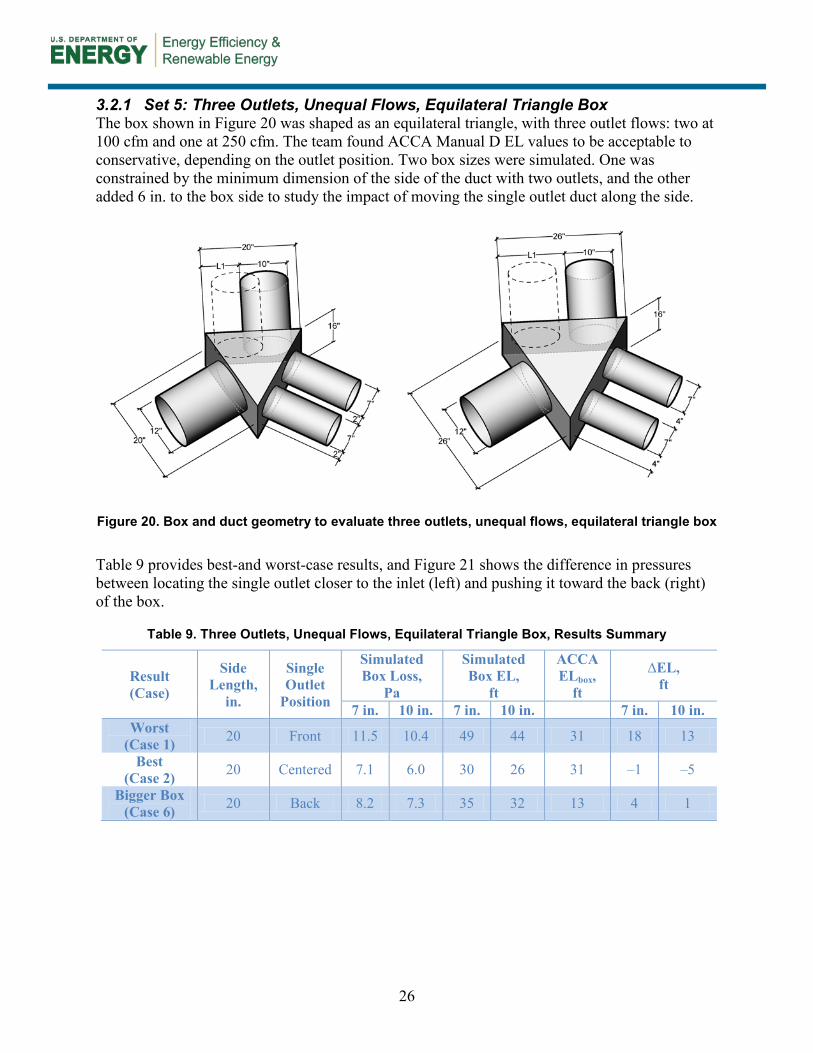
3.2.1 Set 5: Three Outlets, Unequal Flows, Equilateral Triangle Box The box shown in Figure 20 was shaped as an equilateral triangle, with three outlet flows: two at 100 cfm and one at 250 cfm. The team found ACCA Manual D EL values to be acceptable to conservative, depending on the outlet position. Two box sizes were simulated. One was constrained by the minimum dimension of the side of the duct with two outlets, and the other added 6 in. to the box side to study the impact of moving the single outlet duct along the side.

Figure 20. Box and duct geometry to evaluate three outlets, unequal flows, equilateral triangle box

Table 9 provides best-and worst-case results, and Figure 21 shows the difference in pressures between locating the single outlet closer to the inlet (left) and pushing it toward the back (right) of the box.

Table 9. Three Outlets, Unequal Flows, Equilateral Triangle Box, Results Summary

Result (Case)

Side Length,

in.

Single Outlet

Position

Simulated Box Loss,

Pa

Simulated Box EL,

ft

ACCA ELbox,

ft

∆EL, ft

7 in. 10 in. 7 in. 10 in. 7 in. 10 in. Worst

(Case 1) 20 Front 11.5 10.4 49 44 31 18 13

Best (Case 2) 20 Centered 7.1 6.0 30 26 31 –1 –5

Bigger Box (Case 6) 20 Back 8.2 7.3 35 32 13 4 1

27

Figure 21. Midplane pressure gradients for three outlets, unequal flows, equilateral triangle box

3.2.2 Set 6: Three Outlets, Equal Flows, Isosceles Triangle Box Set 6 was similar to Set 5; however, in Set 6, the box was shaped as an isosceles triangle, as shown in Figure 22. The dashed outlet ducts represent the alternate outlet location’s limit. The team sought to achieve three equal flows, totaling 30 cfm (3 × 10 sfm), 300 cfm (3 × 100 cfm), and 750 cfm (3 × 250 cfm). Duct diameters increased to account for the higher flow, and the box dimensions were modified slightly to accommodate the larger inlet and outlet duct sizes.

Figure 22. Box and duct geometry to evaluate three outlets, equal flows, isosceles triangle box

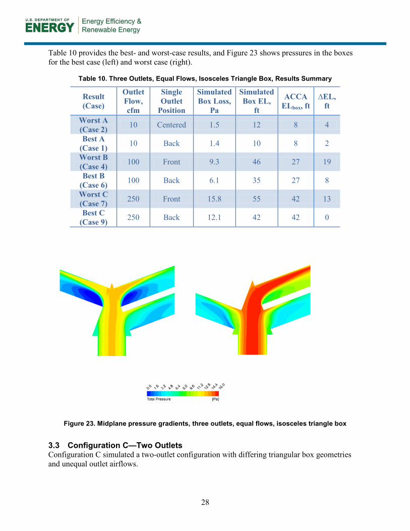
28

Table 10 provides the best- and worst-case results, and Figure 23 shows pressures in the boxes for the best case (left) and worst case (right).

Table 10. Three Outlets, Equal Flows, Isosceles Triangle Box, Results Summary

Result (Case)

Outlet Flow, cfm

Single Outlet

Position

Simulated Box Loss,

Pa

Simulated Box EL,

ft ACCA

ELbox, ft ∆EL,

ft

Worst A (Case 2) 10 Centered 1.5 12 8 4

Best A (Case 1) 10 Back 1.4 10 8 2

Worst B (Case 4) 100 Front 9.3 46 27 19 Best B

(Case 6) 100 Back 6.1 35 27 8

Worst C (Case 7) 250 Front 15.8 55 42 13 Best C

(Case 9) 250 Back 12.1 42 42 0

Figure 23. Midplane pressure gradients, three outlets, equal flows, isosceles triangle box

3.3 Configuration C—Two Outlets Configuration C simulated a two-outlet configuration with differing triangular box geometries and unequal outlet airflows.

29

3.3.1 Set 7: Two Outlets, Unequal Flows, Equilateral Triangle Box Figure 24 shows the configuration with two outlets receiving 100 and 250 cfm, respectively. The dashed ducts represent alternate locations of outlet ducts. The team simulated one 16-in. and one 24-in. equilateral triangular box to evaluate the relative impact of asymmetrical flows and outlet position in the box. The depth was 16 in. for both boxes. Table 11 shows that generally locating outlets as far from the inlet as possible yielded lower pressure losses. Abushakra et al. (2002) found that ACCA Manual D EL values were reasonable for boxes that were sized to exactly fit the inlet and outlet duct sizes. The losses were found to be higher than the ACCA Manual D values and the EL of a traditional sheet metal wye fitting. Despite an asymmetrical flow target, the need for balancing was minimal. Figure 25 shows pressure gradients at the midplane of two Set 7 cases, highlighting the negative effect of locating outlets near the inlet (right) versus far (left).

Figure 24. Box and duct geometry to evaluate two outlets, unequal flows, equilateral triangle box

Table 11. Two Outlets, Unequal Flows, Equilateral Triangle Box, Results Summary

Result (Case)

Side Length,

in.

L1, in.

L2, in.

Simulated Box Loss,

Pa

Simulated Box EL,

ft

ACCA ELbox,

ft

∆EL, ft

7 in. 10 in. 7 in. 10 in. 7 in. 10 in. Worst

(Case 1) 24 15 12 4.9 3.9 34 27 35 –1 –8

Best (Case 2) 24 2 2 8.1 7.1 57 50 35 22 15

Smaller Box (Case 6) 24 7 – 5.9 4.9 41 34 35 6 –1

30

Figure 25. Midplane pressure gradient for two outlets, unequal flows, equilateral triangle box

7” 10” 10” 7”

31

4 Discussion

This report frames its discussion around how the pressure drops calculated in CFD simulations compare to ACCA Manual D EL values and how different configurations perform better or worse than each other. The hypothesis was that in junction boxes, their flexible constraints create a wider range of EL than presented in ACCA Manual D, and better insight into the effects of other parameters, such as box size, will result in better performance of systems using these fittings. One goal was to determine whether variations found in the simulations are significant enough to warrant adjustment to the current model employed by ACCA Manual D for junction boxes or could lead to generalized best practice for the use of junction boxes.

It is important for the ACCA Manual D EL numbers to be conservative to favor oversizing the blower to meet the overall airflow requirements of the system. ACCA further recommends that balancing dampers should be installed in all runs to add the resistance needed to match the fan power with the available pressure and desired airflow to each room.

Given the simulation time necessary, the team selected a limited range of representative airflows as discussed in Section 2.3.2. Discussion of each configuration is presented below, and general recommendations can be found in the Conclusions section.

4.1 Configuration A—Four Outlets 4.1.1 Set 1: Four Outlets with an Entrance Diffuser In small boxes, the use of the “straight” entrance diffuser lowered calculated pressure losses between 10 and 20% compared to other cases. However, this reduction was not to the degree found by Gilman et al. (1951). This indicates the specificity of entrance diffuser design is important and must be adjusted to specific box configurations. As it stands, if a junction box is not built within a 3-ft wide and 3-ft to 8-ft long range, as studied by the Gilman team, it will not perform as effectively. As shown by the differences in results between the “spread” and “straight” fittings simulated in this study, the performance is highly sensitive to fitting geometry, which is difficult to fabricate precisely on site by a contractor.

Also of note are the differences between cases with and without an outlet directly opposite the inlet. Placing an outlet directly opposite the inlet contributes to significantly higher balancing and thus higher box pressure drop. Indicative of performance differences, the magnitude of variation among individual outlet pressures indicates the amount of balancing needed to make all outlets the same. With an outlet opposite the inlet, this pressure difference was consistently greater than in cases with outlets only on the sides, indicating much higher balancing pressures. This result is the justification of the three recommended configurations tested, none of which has an outlet opposite the entrance.

4.1.2 Set 2: Four Outlets, Equal Flows The research team found that, although varying the outlet locations on a box with four outlets with the intent to achieve equal airflow to each outlet did significantly impact the calculated EL of the box, an 8-in. space between the inlet and outlet, with the outlets placed close together, yielded EL values within 5 ft of ACCA Manual D values. Placing the first outlets close to the inlet yielded significantly higher pressures upwards of 15 additional feet of EL, marking a downward pressure trend as the distance from the inlet to the first outlet increases. This is

32

parallel to the ACCA Manual D requirement for a distance of two times the outlet duct diameter between the inlet and the first outlet. Twice the diameter may be a conservative estimate. Also, the optimal distance and spacing will differ for every configuration, and a twice-the-diameter rule should account for all configurations as a conservative value. The simulations marked a significant drop in EL with less than the ACCA Manual D requirement for distance, and any additional distance would likely have yielded little or no additional benefit; however, this is only for limited configurations. Further tests would need to be done to precisely confirm the rule for all possible boxes but would likely be reasonably close to or less than twice the diameter. Pressure losses varied little with an increased space between the two outlets.

Making the box wider induced stability in the system and eliminated balancing. Currently, there are no width recommendations for ACCA Manual D Group 11 fittings. It appears that widening the box to at least twice the inlet diameter could be a recommended practice for more stable flow rates.

4.1.3 Set 3: Four Outlets, Unequal Flows The team found that in boxes where the desired airflows are asymmetrical in a minimally sized box, calculated EL values are above ACCA Manual D EL values. Ducts near the end of the box will receive proportionally more air than any near the inlet, as would be expected. The lowest calculated EL was found in Case 2, where the outlet with a larger friction rate was taken closest to the rear of the box. Case 4, with higher flow outlets at the back, did not require balancing.

All cases were within a reasonable range of pressure, despite differing outlet layouts. Case 2 and Case 4 employed left-to-right symmetry; front to back, they were asymmetrical. This created more predictable flows, although not necessarily lower pressure drops. Although the total pressures were not lower with left-to-right symmetry, balancing was lower. Left-to-right symmetry will yield more predictable results and produce a more self-balancing system. Novel asymmetrical layouts, although possibly optimal, are difficult to predict and therefore are not recommended.

4.1.4 Set 4: Four Outlets, Equal Flows, High Velocities All cases—except Case 2, which performed well below the ACCA Manual D estimate—were found to have higher calculated EL values compared to the ACCA Manual D EL values. The difference was less pronounced in the lower volume, lower velocity cases (Case 1 and Case 2). ACCA Manual D seems to predict EL better for higher velocity and higher resistance junction boxes. This could be due to the higher flow inducing more back pressure into the box and thus more efficiently splitting the air.

The results of Set 4 indicate further analysis should be undertaken for small distributed systems using “pancake” fan coil units, as are common with mini-split or hydronic systems. ACCA Manual D provides little guidance for very small plenum configurations with multiple branch ducts. The fact that these duct runs may be very short also may impact the EL values.

In high friction rate systems such as small-diameter homerun systems, box loss is a much smaller percentage of the total system pressure. For a large increase in total system pressure, such as a 3.3 times increase between Case 1 and Case 2, the box loss increased by only 1.6. This indicates that for high velocity systems, junction boxes can be reasonable choices for fittings.

33

4.2 Configuration B—Three Outlets The ACCA Manual D EL values of triangular boxes configured to split flows three ways were generally reasonable or conservative compared to the calculated EL values. Box size, triangle shape, and the distance of the single duct from the back of the box create variations from the ACCA Manual D EL values. The lowest calculated EL values are highly dependent on all three variables.

4.2.1 Set 5: Three Outlets, Unequal Flows, Equilateral Triangle Box The team found that locating the single duct either in the center or as close to the back of the larger box as possible yielded almost identical calculated EL values, approximately equal to the ACCA Manual D EL values. On the smaller box, the lowest calculated EL value was found to occur when the single duct was centered with a calculated EL value lower than the ACCA Manual D value. The smaller box performed better than the larger one with the outlets farther from the inlet, suggesting that in triangular boxes, larger boxes do not necessarily benefit performance. Balancing was relatively high in all cases—10%–20% additional pressure. Case 2 performed best because it required the least amount of balancing.

4.2.2 Set 6: Three Outlets, Equal Flows, Isosceles Triangle Box Set 6 studied variations in velocity and airflow in a box shaped like an isosceles triangle. As was found in Set 4, small-diameter ducts with lower velocities and lower airflows yielded poorer agreement with ACCA Manual D. Similar to all other sets, placing inlets (Case 3, Case 6, and Case 9) toward the back of the box yielded the lowest pressures.

4.3 Configuration C—Two Outlets The final configuration studied two unequal flows in a box shaped like an equilateral triangle. The team studied this configuration because it is one that is prevalent in the industry.

4.3.1 Set 7: Two Outlets, Unequal Flows, Equilateral Triangle Box The team found that the ELs of the small boxes with outlets placed at the back were reasonably represented by ACCA Manual D. Other configurations were found to have EL values 17%–63% higher (5–27 ft of additional EL) than ACCA Manual D. The larger box size in this configuration had significant benefit in performance, which was not the case in the three-outlet configuration. Note that a metal wye fitting (ACCA Manual D fitting “9O”) has an EL value of 15 at 900 fpm, 0.08 IWC, compared to the 95 EL value for the splitter box (fitting Group 11 at the same reference airspeed and friction rate). For simple splitting of airflow, the wye fitting is a much better choice.

34

5 Conclusions

Designers should recognize that although junction boxes are economical from a first-cost perspective, they add more pressure to systems compared to trunk and branch designs. This pressure drop must be accounted for in the design of the duct system and may result in the need for larger duct sizes compared to those in a trunk and branch system.

In general, this research proposed that through further constraining current design limits provided in ACCA Manual D, Appendix 3, Group 11, better airflow control, stable airflow, and minimized pressure losses could be more consistently achieved by contractors who install flex duct junction box fittings.

The following research questions were asked as part of this project:

• How can current junction box design standards be augmented?

• How do individual geometric parameters affect the proportions and losses of airflow in rectilinear and triangular junction boxes serving two to four discrete rooms?

• How conservative are current ACCA Manual D, Appendix 3, Group 11 guidelines for designing flexible duct junction boxes?

• How do junction boxes perform when outlet duct diameters correspond to the lower room loads of high performance homes?

5.1 How Can Current Junction Box Design Standards Be Augmented? Group 11 fittings could be further elaborated upon to discuss various configurations and flow splits with corresponding EL values. This would provide practitioners with better guidance and the ability to compare EL values with other specific ACCA Manual D, Appendix 3 fittings. In Section 5.2, IBACOS has provided initial guidance based on results of this research.

5.2 How Do Individual Geometric Parameters Affect the Proportions and Losses of Airflow in Rectilinear and Triangular Junction Boxes Serving Two to Four Discrete Rooms?

The “two-diameter to first outlet” rule comes into question. The IBACOS team found that absolute pressure losses attributable to the box do trend downward as the distance increases between the inlet and the first outlet. The relative difference in pressure appears to be overly conservative, given the actual level of precision in the ACCA Manual D process. This causes junction boxes to be sized larger than necessary. Smaller boxes not fully implementing a “twice-the-diameter” rule will save on materials. Width seems to be more important to reduce overall pressure losses in the box than the distance from the inlet to the first outlet. Furthermore, it is easier to use width as the driving dimensional parameter in triangle boxes.

In rectangular boxes, it is clear that simply not having an outlet directly opposite the inlet is more beneficial to reducing overall system pressure than the presence of the entrance diffuser fitting, especially when cost is considered. The flow into the back outlet was proportionally higher than any other case that the team ran with outlets only on the sides. The entrance fittings are not available prefabricated, and it is expected they would have to be made by the contractors. The configuration of the entrance fitting also was found to have a significant impact on the overall

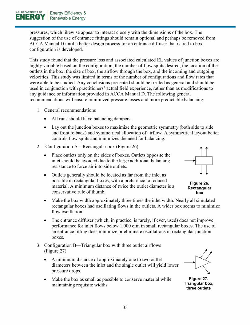
35

pressures, which likewise appear to interact closely with the dimensions of the box. The suggestion of the use of entrance fittings should remain optional and perhaps be removed from ACCA Manual D until a better design process for an entrance diffuser that is tied to box configuration is developed.

This study found that the pressure loss and associated calculated EL values of junction boxes are highly variable based on the configuration, the number of flow splits desired, the location of the outlets in the box, the size of box, the airflow through the box, and the incoming and outgoing velocities. This study was limited in terms of the number of configurations and flow rates that were able to be studied. Any conclusions presented should be treated as general and should be used in conjunction with practitioners’ actual field experience, rather than as modifications to any guidance or information provided in ACCA Manual D. The following general recommendations will ensure minimized pressure losses and more predictable balancing:

1. General recommendations

• All runs should have balancing dampers.

• Lay out the junction boxes to maximize the geometric symmetry (both side to side and front to back) and symmetrical allocation of airflow. A symmetrical layout better controls flow splits and minimizes the need for balancing.

2. Configuration A—Rectangular box (Figure 26)

• Place outlets only on the sides of boxes. Outlets opposite the inlet should be avoided due to the large additional balancing resistance to force air into side outlets.

• Outlets generally should be located as far from the inlet as possible in rectangular boxes, with a preference to reduced material. A minimum distance of twice the outlet diameter is a conservative rule of thumb.

• Make the box width approximately three times the inlet width. Nearly all simulated rectangular boxes had oscillating flows in the outlets. A wider box seems to minimize flow oscillation.

• The entrance diffuser (which, in practice, is rarely, if ever, used) does not improve performance for inlet flows below 1,000 cfm in small rectangular boxes. The use of an entrance fitting does minimize or eliminate oscillations in rectangular junction boxes.

3. Configuration B—Triangular box with three outlet airflows (Figure 27)

• A minimum distance of approximately one to two outlet diameters between the inlet and the single outlet will yield lower pressure drops.

• Make the box as small as possible to conserve material while maintaining requisite widths.

Figure 27. Triangular box,

three outlets

Figure 26. Rectangular

box

36

4. Configuration C—Triangular box with two outlet airflows (Figure 28)

• This fitting is not recommended. A metal wye fitting is significantly better for this purpose.

5.3 How Conservative Are Current ACCA Manual D, Appendix 3, Group 11 Guidelines for Designing Flexible Duct Junction Boxes?

This research did not conclusively quantify how conservative ACCA Manual D EL values are. However, among the cases simulated, the relationship between ACCA Manual D and simulated EL values varied significantly. Factors such as design airflow rates, the nominal duct diameters, and the associated airspeed, as well as the number of ducts, the location of ducts, and the box geometry, result in some simulations showing EL values 50% above adjusted ACCA Manual D EL values; others are very close to ACCA Manual D EL values, and others are overly conservative.

It is important to note that the issues around making the comparison between the simulation results and ACCA Manual D, Group 11 EL values are provided for a single friction rate at a number of different air velocities. In reality, once a nominal duct size is selected for a given air volume, the actual airspeed and friction rate will vary within the inlet duct, the box itself, and each outlet duct. The team chose the highest friction rate and corresponding velocity from the simulation to modify the ACCA Manual D, Group 11 EL values using an equation given in ACCA Manual D, Appendix 3 (p. 146). ACCA Manual D states that “equivalent length values are sensitive to the friction rate and very sensitive to velocity” (p. 146). The team found that once nominal duct diameters had been selected based on a single friction rate, the velocities in the inlet and outlet ducts could vary by up to 300 fpm. This is why the team chose to reiterate the importance of adjusting EL values to specific designed velocities and friction rates.

The ACCA Manual D process adds the effect of balancing dampers in a separate section from calculating total EL; a flat 0.03 IWC (7.47 Pa) is added for each damper (Step 2 of the manual, where component pressure losses are added together). The total component losses are subtracted from the available static pressure of the blower, which is then divided by the total EL to yield a design friction rate. This rate is used to size the ducts to approximate the correct pressure drop across each duct run.

The balancing pressures simulated throughout this study ranged between 0.0 and 0.016 IWC (0–4 Pa). The best configurations had a balancing loss of 0 to approximately 0.006 IWC (0–1.5 Pa). This indicates that if the current ACCA Manual D EL values include some assumed balancing losses, the EL values may be able to be reduced if the designer chooses better configurations.

5.4 How Do Junction Boxes Perform When Outlet Duct Diameters Correspond to the Lower Room Loads of High Performance Homes?

It was observed in low airflow conditions (10–100 cfm, 2–5-in. diameter ducts) that balancing losses were eliminated in all cases. The four-outlet configuration required no balancing to achieve target airflows, with unbalanced outlet flows within 2% of targets. Two of the three cases in the three-outlet configuration required some balancing, but one case was within 10% of

Figure 28. Triangular box,

two airflows

37

the design targets. Balancing losses generally increased with airflow rate, even when outlet velocity was the same. The limited number of configurations evaluated with smaller duct diameters found some to have a fairly large discrepancy as a percentage difference from ACCA Manual D EL values adjusted for flow and velocity; however, the absolute differences are not large enough to make much difference in the duct design process, given the overall level of precision in the ACCA Manual D process.

5.5 Future Research The IBACOS team will seek to validate the CFD simulations against new experimental data to confirm the trend that ACCA Manual D effectively represents actual pressures of these systems. Generally, the CFD simulations trended to having higher pressures and therefore higher adjusted EL values using the equations given in ACCA Manual D, especially with lower airflows. This indicates a potential need for an additional adjustment to EL based on flow volume as well as velocity and friction rate.

More precisely, prefabricated junction boxes could be developed as low cost but high quality fittings. For example, a manufacturer could preconfigure and cut optimal designs that can be folded and quickly taped together on site. This would eliminate discrepancies between the time needed to ensure quality fabrication and well-performing layouts.

Additionally, future research may look into new models for designing junction boxes that may more specifically account for the individual parameters and allow for a wider variety of configurations. From an efficiency standpoint, conservative values lead to higher energy consumption. A more precise EL calculation will result in a lower fan power or speed, resulting in saved energy while still meeting the required flow rates. This is especially important in low-load homes where optimized performance is a goal.

38

References

Abushakra, B.; Dickerhoff, D.; Walker, I.; Sherman, M. (2002). Laboratory Study of Pressure Losses in Residential Air Distribution Systems. Berkeley, CA: Lawrence Berkeley National Laboratory. Report LBNL-49293.

ASHRAE. (2012). 2012 ASHRAE Handbook: HVAC Applications. Atlanta, GA: ASHRAE.

Gilman, S.F.; Martin, R.J.; Konzo, S. (1951). Investigation of the Pressure Characteristics and Air Distribution in Box-Type Plenums for Air Conditioning Duct Systems. University of Illinois Engineering Experiment Station Bulletin, No. 393, 1951 University of Illinois Archives, Record Series Number 11/2/801. Urbana, IL: University of Illinois at Urbana-Champaign. https://www.ideals.illinois.edu/handle/2142/4424.

IECC. (2012). 2012 International Energy Conservation Code. Washington, DC: International Code Council.

Liu, W.; Long, Z.; Chen, Q; (2012). “A Procedure for Predicting Pressure Loss Coefficients of Duct Fittings Using CFD (RP-1493).” HVAC&R Research 18(6): 1168–1181(14).

Moody, L.F. (1944). “Friction Factors for Pipe Flow.” Transactions of the ASME 66(8): 671–684. www.chem.mtu.edu/~fmorriso/cm310/MoodyLFpaper1944.pdf.

Mumma, S.A.; Mahank, T.A.; Ke, Y-P. (1998). “Analytical Determination of Duct Fitting Loss Coefficients.” Applied Energy 61(4): 229–247.

Ridouane, E.H. (2010). “Numerical Evaluation of Indoor Air Distribution in High Performance Homes.” Presented at Residential Building Energy Efficiency Meeting 2010, July 21, 2010. http://apps1.eere.energy.gov/buildings/publications/pdfs/building_america/ns/b23_indoor_air_distr.pdf.

Ridouane. E.H.; Gawlik, K. ( 2011). “Prediction of Air Mixing from High Sidewall Diffusers in Cooling Mode.” Preprint. Golden, CO: National Renewable Energy Laboratory. NREL/CP-5500-49010.

Rutkowski, H. (2006). Manual J—Residential Load Calculation, 8th edition, Version 2. Arlington, VA: Air Conditioning Contractors of America.

Rutkowski, H. (2009). Manual D—Residential Duct Systems, 3rd edition, Version 1.00. Arlington, VA: Air Conditioning Contractors of America.

Shao, L.; Riffat, S.B. (1995). “Accuracy of CFD for Predicting Pressure Losses in HVAC Duct Fittings.” Applied Energy 51: 233–248.

39

Appendix A: Detailed Results

This appendix documents the simulation inputs and results for each set. Each set is documented similarly, consisting of two tables.

The first table in each set includes the fully developed losses of the inlet and outlet ducts present in all cases from the set. This includes simulated flow values and duct diameters and variables for calculating the friction factor per Equation 3 and Equation 4.

The second table in each set contains simulation results and the box loss calculations per Equation 5, the conversion to EL from pressure using Equation 7, and the comparable EL values from ACCA Manual D adjusted using Equation 6 to the maximum friction rate and velocity in the simulation from the reference values in the manual. The first columns in the second table identify each case number and any parameters that are changing between cases. The next columns document the measurements taken from the CFD simulations through to the calculated box losses and EL values. Finally, the ACCA Manual D comparable values are noted, along with the difference between the simulations and ACCA Manual D. Positive values in the last two columns indicate potential additional pressure not accounted for by ACCA Manual D that could be present in systems installed with the given configuration, dimensions, and flows.

Set 1: Four and Five Outlets with an Entrance Diffuser Gilman et al. (1951) described an entrance fitting as diagrammed in Figure 3 as greatly increasing performance in junction boxes. Comparisons were made between boxes with and without the fitting. In addition, two “spreads” were used to test if either performed better. Initial results in a box similar to that in Set 1 with four outlets—two on each side of a rectangle—did not yield a significant reduction in pressure, and a hypothesis was that the results in the Gilman study were so dramatic because there was an outlet out the back of the box. Thus, with the same outlet flows, an additional outlet was placed at the back, and the inlet flow increased by the additional outlet’s flow. Rectangular and circular inlet ducts were used because the design of the fitting aligned better with a rectilinear profile. The outer edges of the circular duct caused the turning to be less pronounced because most of the flow was concentrated in the center vanes. The detailed, fully developed loss calculation inputs and results for Set 1 are presented in Table 12. Table 13 details the inputs and results from the simulations of Set 1.

Table 12. Set 1: Four and Five Outlets with an Entrance Diffuser, Fully Developed Losses

Inlet B 16 1,125 806 108,984 0 0.000 0.018 0.0537 16 0.0007 0.2

InletA 16 900 645 87,188 0 0.000 0.019 0.0359 16 0.0005 0.1

Outlet 10 225 413 34,875 0 0.000 0.023 0.0289 200 0.0048 1.2

Flow

, cfm

Diam

eter

, in.

ID

Loss

Rat

e, IW

C/

100

ft

Fric

tion

Fact

or

k/d

Roug

hnes

s

Reyn

olds

Velo

city

, fpm

Loss

, Pa

Loss

, IW

C

Leng

th, i

n.

40

Table 13. Set 1: Four and Five Outlets with an Entrance Diffuser, Detailed Results

Front Back End Front Back End Front Back End Front Back End

1 None Pipe 155.7* 294.3* – 12.3* 10.7* 8.1* – 8.6* 6.3* – 96* 70* –

(225) (225) –

2 Spread Pipe 231.3 218.7 – 15.6 12.7 13.0 – 11.4 11.7 – 128 131 –

(225) (225) –

3 Straight Pipe 225.0 225.0 – 12.4 9.7 9.7 – 8.4 8.4 – 94 94 –

(225) (225) –

4 Spread Square 248.9 201.2 – 16.9 13.5 14.7 – 12.2 13.4 – 137 150 –

(225) (225) –

5 Straight Square 234.5 215.6 – 12.9 9.9 10.4 – 8.6 9.1 – 96 102 –

(225) (225) –

6 None Pipe 140.6 272.3 299.3 15.2 14.1 11.0 10.2 12.7 9.7 8.8 95 72 66

(225) (225) (225)

7 None Square 149.5 264.1 297.8 15.8 14.5 11.9 10.8 13.1 10.5 9.5 98 79 71

(225) (225) (225)

8 Spread Pipe 173.1 218.0 342.8 17.6 16.0 15.1 11.5 14.6 13.7 10.2 109 102 76

(225) (225) (225)

9 Straight Pipe 182.1 241.6 277.6 14.1 12.3 11.0 10.0 11.0 9.6 8.6 82 72 64

(225) (225) (225)

10 Spread Square 172.3 215.1 350.2 19.4 17.7 16.8 12.7 16.4 15.5 11.3 122 116 85

(225) (225) (225)

11 Straight Square 180.0 222.8 319.5 13.8 12.0 11.1 8.2 10.7 9.7 6.9 80 73 51

(225) (225) (225)

Unbalanced Box EL, ftUnbalanced Box Loss, PaTotal Pressure, Pa

(Target Flow, cfm)

Unbalanced Flow, cfm

Pres

sure

at

Inlet

, Pa

Inlet

Pro

file

Fitt

ing

Cas

e

*Oscillatory result.

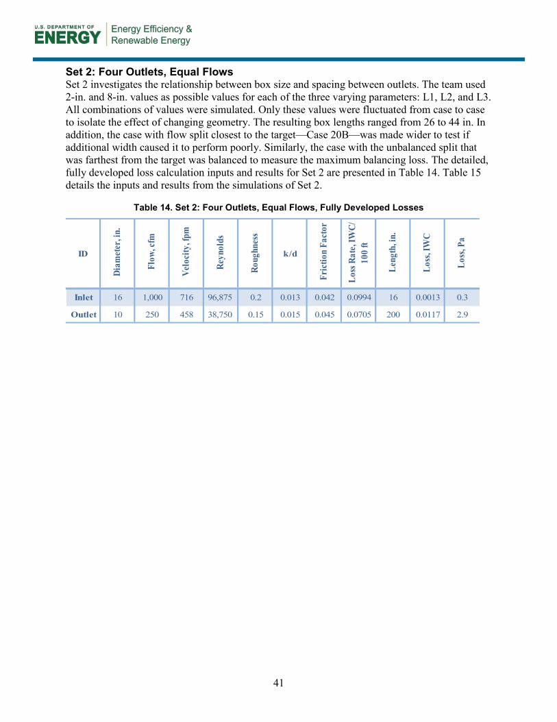
41

Set 2: Four Outlets, Equal Flows Set 2 investigates the relationship between box size and spacing between outlets. The team used 2-in. and 8-in. values as possible values for each of the three varying parameters: L1, L2, and L3. All combinations of values were simulated. Only these values were fluctuated from case to case to isolate the effect of changing geometry. The resulting box lengths ranged from 26 to 44 in. In addition, the case with flow split closest to the target—Case 20B—was made wider to test if additional width caused it to perform poorly. Similarly, the case with the unbalanced split that was farthest from the target was balanced to measure the maximum balancing loss. The detailed, fully developed loss calculation inputs and results for Set 2 are presented in Table 14. Table 15 details the inputs and results from the simulations of Set 2.

Table 14. Set 2: Four Outlets, Equal Flows, Fully Developed Losses

Inlet 16 1,000 716 96,875 0.2 0.013 0.042 0.0994 16 0.0013 0.3

Outlet 10 250 458 38,750 0.15 0.015 0.045 0.0705 200 0.0117 2.9

Roug

hnes

sID

Diam

eter

, in.

Flow

, cfm

Velo

city

, fpm

Reyn

olds

k/d

Fric

tion

Fact

or

Loss

Rat

e, IW

C/

100

ft

Leng

th, i

n.

Loss

, IW

C

Loss

, Pa

42

Table 15. Set 2: Four Outlets, Equal Flows, Detailed Results

W L1 L2 L3 Front Back Front Back Front Back Front Back Front Back Back Front

1 20 2 2 2 222.5* 277.5* 22.7* – 3.2 3.2 – – 19.5* 19.5* – 16.3* 16.3* – 66* 66* 66 51 15 31%

(250) (250)

2 20 8 2 2 248.5* 251.5* 20.2* – 3.6 3.4 – – 16.6* 16.8* – 13.3* 13.5* – 54* 55* 55 51 4 9%

(250) (250)

3 36 8 2 2 248.5 251.5 19.7 – 3.5 3.6 – – 16.2 16.1* – 12.97 12.9* – 52 52 52 51 1 3%

(250) (250)

4 20 8 8 2 240* 260* 19.2* – 3.3 3.8 – – 16.4* 15.4* – 13.1* 12.1* – 53* 49* 53 51 2 5%

(250) (250)

5 20 8 8 8 223.5* 276.5* 18* – 2.8 4.3 – – 15.5* 13.7* – 12.3* 10.4* – 50* 42* – 51 – –

(250) (250)

6 20 2 8 8 210* 290* 19* – 2.5 4.8 – – 16.6* 14.2* – 13.4* 11* – 54* 44* – 51 – –

(250) (250)

7 20 2 2 8 204.5* 295.5* 19.3* 22.7 2.4 4.9 3.5 3.2 15.8* 14.4* 15.9 12.5* 11.1* 15.9 51* 45* 64 51 14 27%

(250) (250)

8 20 8 2 8 224.5* 275.5* 18.3* – 2.9 4.2 – – 15.4* 14.1* – 12.1* 10.8* – 49* 44* – 51 – –

(250) (250)

9 20 2 8 2 228.5* 271.5* 21.1* – 3.0 4.2 – – 18.1* 16.9* – 14.9* 13.7* – 60* 55* 60 51 9 19%

(250) (250)

Bal

ance

d B

ox L

oss,

Pa

Bal

ance

d

ΔE

L, f

t

ΔE

L, %

Cas

e

Outlet Pressure, PaInlet Pressure,

Pa

Bal

ance

d B

ox E

L, f

t

AC

CA

EL

, ft

Unb

alan

ced

Bal

ance

d

BalancedUnbalanced

Total Pressure, Pa Unbalanced Box EL, ft

Unbalanced Box Loss, Pa

Unbalanced

Unbalanced Flow, cfm

(Target Flow, cfm)

Dimensions, in.

*Oscillatory result.

43

Set 3: Four Outlets, Unequal Flows Set 3 examines the effects of pressure at the inlet when the relative outlet locations of an asymmetrical condition are varied. This experiment is driven by the likelihood of balancing losses increasing when higher flow outlets are located before lower flow outlets, due to the preference of the air to flow into the rear outlets. The centerlines of the outlet ducts, the inlet flow rate, and the box dimensions were held constant between cases. The detailed, fully developed loss calculation inputs and results for Set 3 are presented in Table 16. Table 17 details the inputs and results from the simulations of Set 3.

Table 16. Set 3: Four Outlets, Unequal Flows, Fully Developed Losses

Inlet 16 1,000 716 96,875 0.2 0.013 0.042 0.0994 16 0.0013 0.3

Outlet A 7 100 374 22,143 0.2 0.029 0.058 0.0859 200 0.0143 3.6

Outlet B 10 250 458 38,750 0.2 0.020 0.050 0.0779 200 0.0130 3.2

Loss

, IW

C

Loss

, Pa

k/d

Fric

tion

Fact

or

ID

Diam

eter

, in.

Flow

, cfm

Velo

city

, fpm

Reyn

olds

Loss

Rat

e, IW

C/

100

ft

Leng

th, i

n.

Roug

hnes

s

44

Table 17. Set 3: Four Outlets, Unequal Flows, Detailed Results

FL BL BR FR FL BL BR FR FL BL BR FR 7 10 7 10 7 10 7 10

1 7 7 10 10 101.5 118.3 268.1 212.1 16.8 18.8 16.5 16.5 15.6 15.3 12.6 11.8 63 62 51 12 11 24% 22%

(112) (112) (238) (238) (7) (7) (10) (10)

(100) (100) (250) (250)

2 10 7 7 10 225.4 124.6 124.6 225.4 17.5 18.7 15.9 15.1 15.1 15.9 11.2 12.3 61 64 51 10 14 21% 27%

(238) (112) (112) (238) (10) (7) (7) (10)

(250) (100) (100) (250)

3 10 7 10 7 197.4 139.3 266.7 91.7 15.8 18.6 15.2 16.4 15.0 16.3 12.4 11.4 61 66 51 10 15 20% 30%

(238) (112) (238) (112) (10) (7) (10) (7)

(250) (100) (250) (100)

4 7 10 10 7 105.0 245.0 245.0 105.0 19.5 20.0 17.6 16.6 16.6 17.7 13.8 13.0 67 71 51 16 21 33% 41%

(112) (238) (238) (112) (7) (10) (10) (7)

(100) (250) (250) (100)

Bala

nced

Unb

alan

ced

AC

CA

EL,

ft

ΔEL,

%

ΔEL,

ft

Bala

nced

Box

EL,

ft

Balanced Total Pressure, Pa

(Diameter, in.) Bala

nced

Box

Los

s, PaInlet

Pressure, Pa

Cas

e

Outlet Diameters, in. Unbalanced Flow, cfm

(Natural Flow, cfm)

(Target Flow, cfm)

45

Set 4: Four Outlets, Equal Flows, High Velocities Set 4 was designed to compare the differences in pressure loss through a junction box when the outlet diameters decrease, resulting in higher velocities and friction rates. The inlet diameter, the flow rate, and the box dimensions remained constant. Three flow rates were tested with two outlet diameters each. Flow was split into four outlets and balanced to achieve equal flow into each outlet, and the losses attributed to the box were calculated. The detailed, fully developed loss calculation inputs and results for Set 4 are presented in Table 18. Table 19 details the inputs and results from the simulations of Set 4.

Table 18. Set 4: Four Outlets, Equal Flows, High Velocities, Fully Developed Losses

Inlet 1 5 40 293 12,400 0.09 0.018 0.050 0.0642 60 0.0032 0.8

Outlet A 2 10 458 7,750 0 0.000 0.033 0.2598 200 0.0433 10.8

Outlet B 3 10 204 5,167 0 0.000 0.037 0.0382 200 0.0064 1.6

Inlet 2 12 400 509 51,667 0.18 0.015 0.045 0.0720 60 0.0036 0.9

Outlet 5 100 733 31,000 0.09 0.018 0.048 0.3858 200 0.0643 16.0

Outlet C 7 100 374 22,143 0.12 0.017 0.048 0.0713 200 0.0119 3.0

Inlet 3 16 1,000 716 96,875 0.2 0.013 0.042 0.0994 60 0.0050 1.2

Outlet D 7 250 935 55,357 0.2 0.029 0.057 0.5286 200 0.0881 21.9

Outlet E 10 250 458 38,750 0.15 0.015 0.045 0.0705 200 0.0117 2.9

k/d

Fric

tion

Fact

or

Loss

Rat

e, IW

C/

100

ft

Leng

th, i

n.

Loss

, IW

C

Loss

, Pa

ID

Diam

eter

, in.

Flow

, cfm

Velo

city

, fpm

Reyn

olds

Roug

hnes

s

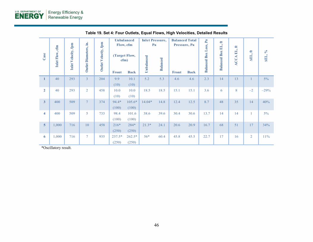
46

Table 19. Set 4: Four Outlets, Equal Flows, High Velocities, Detailed Results

Front Back Front Back

1 40 293 3 204 9.9 10.1 5.2 5.3 4.6 4.6 2.3 14 13 1 5%

(10) (10)

2 40 293 2 458 10.0 10.0 18.5 18.5 15.1 15.1 3.6 6 8 –2 –29%

(10) (10)

3 400 509 7 374 94.4* 105.6* 14.04* 14.8 12.4 12.5 8.7 48 35 14 40%

(100) (100)

4 400 509 5 733 98.4 101.6 38.6 39.6 30.4 30.6 13.7 14 14 1 5%

(100) (100)

5 1,000 716 10 458 216* 284* 21.3* 24.1 20.6 20.9 16.7 68 51 17 34%

(250) (250)

6 1,000 716 7 935 237.5* 262.5* 56* 60.4 45.8 45.5 22.7 17 16 2 11%

(250) (250)

Bal

ance

d Bo

x Lo

ss, P

a

Bal

ance

d Bo

x EL

, ft

AC

CA

EL,

ft

ΔEL

, ft

ΔEL,

%

Unb

alan

ced

Bala

ncedC

ase

Inlet

Flo

w, c

fm

Inlet

Velo

city,

fpm

Out

let D

iam

eter

s, in

.

Out

let V

eloct

iy, f

pm

(Target Flow, cfm)

Unbalanced Flow, cfm

Inlet Pressure, Pa

Balanced Total Pressure, Pa

*Oscillatory result.

47

Set 5: Three Outlets, Unequal Flows, Equilateral Triangle Box Similar to Set 3, Set 5 explores the effect of greater asymmetry on balancing and total pressure. It also seeks to determine if box performance better aligns with ACCA Manual D data when splitting into three as opposed to four. It is expected that balancing losses will be greater when the split is the most asymmetrical. Two box sizes also were simulated to garner whether box size plays a part in the box loss. Finally, the larger left outlet was shifted along the side of the box to examine the effect of outlet location. The detailed, fully developed loss calculation inputs and results for Set 5 are presented in Table 20. Table 21 details the inputs and results from the simulations of Set 5.

Table 20. Set 5: Three Outlets, Unequal Flows, Equilateral Triangle Box, Fully Developed Losses

Inlet 12 450 573 58,125 0.2 0.017 0.046 0.0944 16 0.0013 0.3

Outlet 10 250 458 38,750 0.2 0.020 0.050 0.0779 200 0.0130 3.2

Outlet 7 100 374 22,143 0.2 0.029 0.058 0.0859 200 0.0143 3.6

Roug

hnes

s

ID

Diam

eter

, in.

Flow

, cfm

Velo

city

, fpm

Reyn

olds

k/d

Fric

tion

Fact

or

Loss

Rat

e, IW

C/

100

ft

Leng

th, i

n.

Loss

, IW

C

Loss

, Pa

48

Table 21. Set 5: Three Outlets, Unequal Flows, Equilateral Triangle Box, Detailed Results

RF RB L RF RB L 7 10 7 10 7 10 7 10

1 20 2 101.7* 138.6* 209.3* 13.1* 17.5 15.3 15.4 13.9 11.5 10.4 49 44 31 18 13 58% 43%

(111.5) (111.5) (227)

(100) (100) (250)

2 20 4 88.7* 127.8* 213.8* 11.5* 13.1 10.9 11.0 9.6 7.1 6.0 30 26 31 –1 –5 –2 –17%

(111.5) (111.5) (227)

(100) (100) (250)

3 20 8 91.8* 121.5* 236.7* 11.9* 16.3 13.7 14.1 12.9 10.2 9.4 43 40 31 12 9 40% 29%

(111.5) (111.5) (227)

(100) (100) (250)

4 26 2 88.7 135.0 226.4 11.7 15.7 13.4 13.5 12.1 9.7 8.6 41 37 31 10 6 33% 18%

(111.5) (111.5) (227)

(100) (100) (250)

5 26 8 74.7 119.3 256.1 11.4 14.4 12.2 12.3 10.9 8.5 7.4 36 31 31 5 0 16% 2%

(111.5) (111.5) (227)

(100) (100) (250)

6 26 14 76.5 124.7 248.9 12.8 14.2 12.0 12.0 10.9 8.2 7.3 35 31 31 4 0 12% 1%

(111.5) (111.5) (227)

(100) (100) (250)

ΔEL,

ft

ΔEL,

%

Bala

nced

Box

Los

s, Pa

Bala

nced

Box

Los

s, EL

AC

CA

EL,

ft

Cas

e

L1,

in.

Wid

th, i

n.

Bala

nced

Unb

alan

ced

(Target Flow, cfm)

(Natural Flow, cfm)

Balanced Total Pressure, Pa

Inlet Pressure, Pa

Unbalanced Flow, cfm

*Oscillatory result.

49

Set 6: Three Outlets, Equal Flows, Isosceles Triangle Box Set 6 compares pressure variations as the location of an outlet duct varies. Three flow rates were tested, with each case using the smallest possible junction box while maintaining an isosceles profile. Each flow rate was simulated with two outlets on the right and one on the left. The left outlet was moved within its side to three positions: at the front, centered, and at the back. The detailed, fully developed loss calculation inputs and results for Set 6 are presented in Table 22. Table 23 details the inputs and results from the simulations of Set 6.

Table 22. Set 6: Three Outlets, Equal Flows, Isosceles Triangle Box, Fully Developed Losses

Inlet A 4 30 344 11,625 0.15 0.038 0.063 0.1391 6 0.0007 0.2

Outlet A 3 10 204 5,167 0.15 0.050 0.073 0.0755 60 0.0038 0.9

Inlet B 10 300 550 46,500 0.15 0.015 0.045 0.1010 7 0.0006 0.1

Outlet B 7 100 374 22,143 0.15 0.021 0.052 0.0771 160 0.0103 2.6

Inlet C 14 750 702 83,036 0.2 0.014 0.044 0.1143 14 0.0013 0.3

Outlet C 10 250 458 38,750 0.2 0.020 0.050 0.0779 160 0.0104 2.6

Roug

hnes

s

k/d

Fric

tion

Fact

or

Loss

Rat

e, IW

C/

100

ft

Leng

th, i

n.

ID

Diam

eter

, in.

Flow

, cfm

Velo

city

, fpm

Reyn

olds

Loss

, Pa

Loss

, IW

C

50

Table 23. Set 6: Three Outlets, Equal Flows, Isosceles Triangle Box, Detailed Results

RF RB L RF RB L

1 10 2 8.1 13.3 8.6 4.0 4.7 4.1 4.1 4.1 1.4 12 8 3 38%

(10) (10) (10)

2 10 5 9.4 12.0 8.7 4.3 4.8 4.2 4.2 4.1 1.5 12 8 3 40%

(10) (10) (10)

3 10 7 8.76* 10.32* 10.92* 4.1 4.3 3.7 3.7 3.7 1.0 11 8 2 25%

(10) (10) (10)

4 100 2 72.3 134.4 93.3 10.7 13.9 12.0 11.4 11.5 9.3 46 27 19 71%

(100) (100) (100)

5 100 7 90.9 118.8 90.3 10.5 12.1 9.8 9.9 9.7 7.2 39 27 12 45%

(100) (100) (100)

6 100 11 94.8 103.2 102.0 10.7 11.1 8.8 8.8 8.8 6.1 35 27 8 32%

(100) (100) (100)

7 250 2 240* 286.5* 223.5* 14.2 18.7 14.3 15.8 15.7 15.8 55 42 13 31%

(250) (250) (250)

8 250 8 217.5 297.0 235.5 14.5 16.1 12.6 12.9 12.7 12.9 45 42 3 6%

(250) (250) (250)

9 250 14 238.5 258.0 253.5 15.1 15.5 12.1 12.1 12.1 12.1 42 42 0 1%

(250) (250) (250)

ΔEL

, ft

Balanced Total Pressure, Pa

Inlet Pressure, Pa

Bala

nced

Unb

alan

ced(Target Flow, cfm)

ΔEL,

%

Unbalanced Flow, cfm

Cas

e

Out

let F

low

L1,

in.

Bal

ance

d Bo

x Lo

ss, P

a

Bal

ance

d Bo

x Lo

ss, E

L

AC

CA

Equ

ival

ent

*Oscillatory result.

51

Set 7: Two Outlets, Unequal Flows, Equilateral Triangle Box Aside from a simple symmetrical split into two, Set 7 represents the simplest scenario for a junction box. The locations of the outlets were shifted along the sides of two box sizes to determine if “at the back makes things better” is indeed a universal trend. Box size also was increased to indicate if the larger size and the distance between the inlet and the first outlet improve performance. The detailed, fully developed loss calculation inputs and results for Set 7 are presented in Table 24. Table 25 details the inputs and results from the simulations of Set 7.

Table 24. Set 7: Two Outlets, Unequal Flows, Equilateral Triangle Box, Fully Developed Losses

Inlet 12 350 446 45,208 0.2 0.017 0.046 0.0574 16 0.0008 0.2

Outlet A 10 250 458 38,750 0.2 0.020 0.050 0.0779 200 0.0130 3.2

Outlet B 7 100 374 22,143 0.2 0.029 0.058 0.0859 200 0.0143 3.6

Loss

, Pa

ID

Diam

eter

, in.

Flow

, cfm

Velo

city

, fpm

Reyn

olds

Roug

hnes

s

k/d

Fric

tion

Fact

or

Loss

Rat

e, IW

C/

100

ft

Leng

th, i

n.

Loss

, IW

C

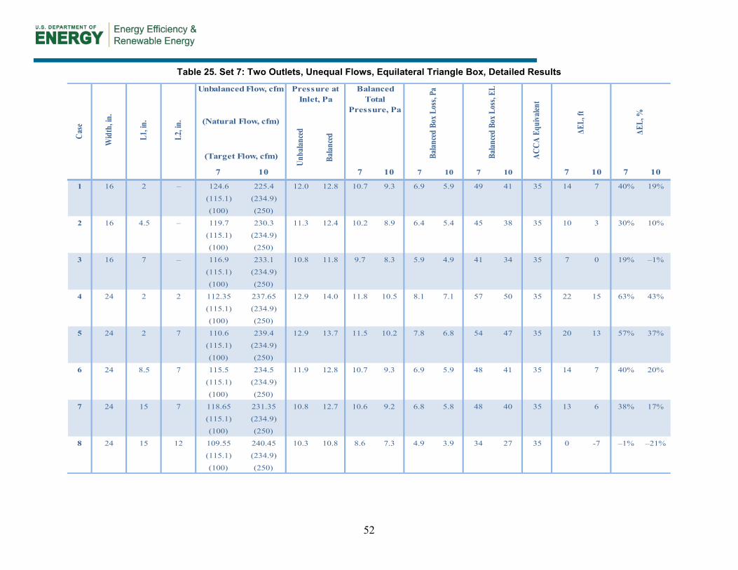
52

Table 25. Set 7: Two Outlets, Unequal Flows, Equilateral Triangle Box, Detailed Results

7 10 7 10 7 10 7 10 7 10 7 10

1 16 2 – 124.6 225.4 12.0 12.8 10.7 9.3 6.9 5.9 49 41 35 14 7 40% 19%

(115.1) (234.9)

(100) (250)

2 16 4.5 – 119.7 230.3 11.3 12.4 10.2 8.9 6.4 5.4 45 38 35 10 3 30% 10%

(115.1) (234.9)

(100) (250)

3 16 7 – 116.9 233.1 10.8 11.8 9.7 8.3 5.9 4.9 41 34 35 7 0 19% –1%

(115.1) (234.9)

(100) (250)

4 24 2 2 112.35 237.65 12.9 14.0 11.8 10.5 8.1 7.1 57 50 35 22 15 63% 43%

(115.1) (234.9)

(100) (250)

5 24 2 7 110.6 239.4 12.9 13.7 11.5 10.2 7.8 6.8 54 47 35 20 13 57% 37%

(115.1) (234.9)

(100) (250)

6 24 8.5 7 115.5 234.5 11.9 12.8 10.7 9.3 6.9 5.9 48 41 35 14 7 40% 20%

(115.1) (234.9)

(100) (250)

7 24 15 7 118.65 231.35 10.8 12.7 10.6 9.2 6.8 5.8 48 40 35 13 6 38% 17%

(115.1) (234.9)

(100) (250)

8 24 15 12 109.55 240.45 10.3 10.8 8.6 7.3 4.9 3.9 34 27 35 0 -7 –1% –21%

(115.1) (234.9)

(100) (250)

Case

Wid

th, in

.

L1,

in.

L2,

in. (Natural Flow, cfm)

(Target Flow, cfm)

Balanced Total

Pressure, Pa

Pressure at Inlet, Pa

Unbalanced Flow, cfm

Unba

lance

d

Balan

ced ΔE

L, ft

ΔEL,

%

Balan

ced

Box L

oss,

Pa

Balan

ced

Box L

oss,

EL

ACCA

Equ

ivalen

t

53

Appendix B: Code Barriers on the Use of Flammable Materials in Space Conditioning Systems, by Duncan Prahl

Background Research cited by Walker (2007) indicates that current fan blower efficiency is roughly 10%–15%, indicating opportunities for more efficient air movement through aerodynamically designed fan blowers. This will become increasingly important if air handler fans also are used for air circulation and ventilation during non-heating or cooling periods. In addition, duct systems could be constructed using lightweight plastic components, which would allow for small diameters that are appropriately sized for lower airflows.

Two ways to achieve energy efficiency that are well documented are bringing ducts inside conditioned space and sealing the duct system (NREL 2005). New and existing homes commonly have duct systems that are in unconditioned attics and are poorly sealed. Conventional solutions to bring ducts inside conditioned space include redesign to integrate ducts in floor spaces, insulating at the underside of the roof deck to create a conditioned attic and leaving the ducts in the attic, creating soffits dropped below the ceiling line, or some combination of these strategies. In addition, space must be found inside the conditioned space for the air handling unit, typically requiring approximately 6 ft2 of floor area.

Codes for new construction have significantly improved, and houses built to the 2012 IECC often have load densities of 900–1,200 ft2/12,000 Btu/h of nominal cooling. This translates to roughly 0.33–0.44 cfm of conditioned air per square foot of living area at peak conditions. This leads to bedroom airflows of 40–100 cfm and aggregate living space airflows of 150–250 cfm.

These realities of new construction are also finding their way into existing homes that are undertaking moderate to deep energy retrofits. Although the load densities are somewhat lower, there remains the problem of downsized air handling equipment being installed in oversized leaky ducts in attics or the difficulty of retrofitting a duct system below the conditioned ceiling, with the associated loss of floor space for the air handler and extensive soffits needed to accommodate ducts from a central HVAC unit.

Past research by Ridouane and Gawlik (2011) has shown that high sidewall interior supply registers can provide good comfort for occupants. Ridouane (2010) showed that 500 and 700 fpm for heating and cooling provides enough momentum for the air to mix in the room. This research also showed that lower temperature air at the outlets in the heating mode is desirable to minimize stratification.

Residential space conditioning equipment typically is one unit for the entire house. Historically, higher-end systems were split into two systems to zone the house but still relied on a central air handler with a duct system that distributes the air throughout the zone. Proper design of duct systems becomes increasingly difficult as the room cfm drops, especially when attempting to keep the system in reasonable balance and have higher supply outlet air velocities to facilitate mixing in the room.

One solution to this problem is to not locate the heating and cooling unit centrally and force the ducts to go throughout the house. Instead, the solution is to break down the heating and cooling

54

system into smaller discrete parts and to allow multiple systems to serve different spaces. This allows for significantly shorter duct runs, low static pressures in the system, and potentially greater use of temperature setup/setback in unoccupied spaces (e.g., bedrooms).

To make this strategy feasible in the United States, two major hurdles must be overcome. The first hurdle is equipment availability and cost, which is less of a technical challenge and more of a market challenge. The second hurdle is finding low-cost, simple, leak-free duct systems that can be modularized to accommodate the necessary flows for each room in increments of approximately 10–15 cfm. Table 26 gives approximate flow rates for various duct diameters.

Table 26. Approximate Flow Rates for Duct Diameters

Duct Diameter (in.)

cfm @ 500 fpm

cfm @ 700 fpm

1.5 6 9 2 11 15 3 25 34 4 44 61 5 68 95 6 98 137

One solution that would achieve the desired ducts is to use readily available plastic plumbing piping. Pipe diameters could be mixed and matched to provide the appropriate airflow for a room, and the solvent welding of joints is inherently airtight. These duct systems have low static pressure and a straight duct roughness. However, polyvinyl chloride plastic pipe currently is approved for use in plumbing systems but not for use in above-grade duct systems.

Code Research A literature search was undertaken to determine the genesis of the duct flammability requirements in the 2012 International Residential Code (IRC 2012). The first codes in the United States were developed by the National Board of Fire Underwriters (NBFU) as a means to encourage the construction of buildings that would not catch fire, and if those buildings did catch fire, it would not spread throughout the building or to other buildings. The history of the first 50 years of the NBFU is well documented by Brearley (1916), and the underlying purpose of the codes was offered by the NBFU (1945). Relative to fire safety in ducted systems, the NBFU published a guide (NBFU 1915) that requires the ducts to be “made of galvanized iron or other approved non combustible material” and recommends that fans be interconnected to fire and smoke alarm systems so that the fans shut down in the event of a fire. Another NBFU publication (NBFU 1935) indicates “recent fires” in metal ducts with flammable linings and that the fire department had a difficult time fighting the fire that was inside the duct system. NBFU (1935) also indicates that “only fire resistive linings acceptable to the inspection department having jurisdiction may be used inside of ducts.”

Brearley (1916) states that electricity was seen as a major new contributor to fires in buildings in the early 1900s, which gave rise to the development of the National Electric Code by the NBFU. Specific recommendations in several NBFU pamphlets imply that either direct sparking or sparks

55

from static electricity generated by fans and belts in ventilation and space conditioning systems is a specific concern that should be avoided, presumably to limit the possibility of fires.

Plastics began to be introduced into the building industry in the 1930s and more aggressively in the 1950s. In 1954, the U.S. Chamber of Commerce held a meeting on the use of plastics in buildings and published a proceedings (Building Research Institute 1955) that contained one section specifically related to plastic duct systems. Skiest (1966) documents the Society of the Plastics Industry’s Code Advisory Committee activities that resulted in the development of the first “Model Chapter on Plastics for Inclusion in Building Codes.” This first Model Chapter language references material classes A (flame spread less than 25), B (flame spread 25 to greater than or equal to 75), C (flame spread 75 to 250), and D (flame spread 250 to 500).

Research on fires within ducts was conducted for the U.S. Department of Mines related to the propagation of fires in wood-lined mine shafts or the propagation of fires within ventilation duct systems for fresh air to mines (Perzak et al. 1987; Lee et al. 1980). Several key findings from this research related to the performance of ducts in residential buildings state that fire did not enter air supply or exhaust outlets in duct systems, provided the opening was an aperture as opposed to a large boot with a supply outlet diffuser. In addition, fires from flammable materials on the inside of the ducts consume the available oxygen in the ducts and create a zone of combustible gases in front of the flame. In addition, Lee et al. (1980) found that the fire creates a pressure regime that can actually overwhelm any fan-induced airflows, even at high velocities. This causes fire to spread toward the fan.

Testing by the Building Research Establishment (2005) suggests that steel return grilles or face dampers help to limit the entry of flame into a duct from a fire source below it. It further suggests that when fans are turned off 2 min after smoke is detected at the air handler, the duct temperatures remained below 70°C (158°F).

Analysis and Interpretation Table 27 summarizes the 2012 IRC (IRC 2012) allowable use of materials with relatively high flame spread and smoke developed rating as surface materials, including up to 10% of the exposed surface area of rooms to use materials with a flame spread less than 75 and unlimited smoke developed. Foam plastic insulation is allowed with a thermal barrier. The interior surface of a duct must meet a flame spread of less than 25 and a smoke developed of less than 50. Table 28 provides a summary of flame spread ratings for several different materials.

56

Table 27. Flame Spread and Smoke Developed Ratings From the 2012 IRC

(IRC 2012) Code Section (IRC 2012)

Flame Spread (ASTM E84)

Smoke Developed (ASTM E84)

R302.9 (Interior Finishes)

200 (unlimited for “trim,” doors and windows and finished 1/28-in. thick adhered to

surface no worse than paper)

450

R302.10 (Insulation) 25 450 R316.3 (Foam Plastic) 75 450

R316.5.9 Plastic Trim (<10% Wall + Ceiling Area) 75 Unlimited

R302.9.4, R316.5.10 Foam Plastic Interior Finish 200 (or pass NFPA 286) 450 (or pass NFPA 286)

M1601.1.1.2 (Factory Made Ducts) 0/25 Not specified M1601.1.1.6 (Duct Systems) 200 Not specified

M1601.1.2 (Underground Ducts, Max. 150°F SAT)

25 (inferred from M1601.3)

50 (inferred from M1601.3)

M1601.3.1 and 2 (Duct Lining/Covering, and Shall Not Flame, Glow, Smolder, Smoke

under ASTM C411)

25 50

Table 28. Flame Spread and Smoke Developed of Common Materials

Material Flame Spread (ASTM E84)

Smoke Developed (ASTM E84)

Red Oak 100 100 Polyvinyl Chloride 10–15 > 300

Gypsum Board 10–15 0

It appears that all of these various requirements have been developed based on specific industry interests (i.e., flexible duct manufacturers, plastic duct manufacturers, foam plastic manufacturers, HVAC equipment manufacturers, gypsum manufacturers). This fragmentation of the code substantially limits the possibility for innovative solutions to be developed and implemented in the industry.

Engineering and fire protection principles indicate the basic assumptions shown in Table 29 that should be followed to limit loss of life (occupants and firefighters) in the event of a house fire.

57

Table 29. Requirements in Various Sections of the 2012 IRC to Limit Loss of Life and Fire Promulgation

(IRC 2012)

Characteristics Least Restrictive Code Limit

Use materials and systems that limit the spread of fire from the location of origin—from the burning object in the room to the rest of room, from a burning room to adjacent rooms, and from a burning building to an

adjacent building.

200 Flame Spread (ASTM E84)

Use materials and systems that limit the development of smoke to enable occupant escape and firefighting

efforts. 450 Smoke Developed

(ASTM E84) Use automatic systems to warn occupants in the event of fire and to help suppress fires before the fires grow

out of control.

Sprinklers and smoke/ carbon monoxide alarms

required Electrical and fuel burning equipment in buildings

should not be the originating source of fire (should not create sparks, excessive heat, etc.).

UL tests

Systems in buildings (e.g., HVAC, structure, plumbing, electrical, thermal, water management, finishes) should not substantially contribute to the

spread of fire, hot gases, or smoke within the building or from building to building.

UL tests, fire blocking, ASTM E84

Recommended Guidance Currently, builders have no choice but to follow code requirements. The IRC could be modified to accommodate various duct materials, as follows:

M1601.1.1 (Revised), M1601.3 (Revised), M1603 (New) Revise as follows: M1601.1.1 Above-ground duct systems. Above-ground duct systems shall conform to the following: 1. Equipment connected to duct systems shall be designed to limit discharge air temperature to a maximum of 250°F (121°C).

2. Factory-made air ducts shall be constructed of Class 0 or Class 1 materials as designated in Table M1601.1.1(1).

Exception: Factory-made air ducts with a flame spread of 25 and a smoke developed of 450 are allowed provided the duct system is provided with smoke detection system control that meets the requirements of Section M1603.

3. Fibrous duct construction shall conform to the SMACNA Fibrous Glass Duct Construction Standards or NAIMA Fibrous Glass Duct Construction Standards.

58

4. Minimum thickness of metal duct material shall be as listed in Table M1601.1.1(2). Galvanized steel shall conform to ASTM A653. Metallic ducts shall be fabricated in accordance with SMACNA Duct Construction Standards Metal and Flexible.

5. Use of gypsum products to construct return air ducts or plenums is permitted, provided that the air temperature does not exceed 125°F (52°C) and exposed surfaces are not subject to condensation.

6. Duct systems shall be constructed of materials having a flame spread index not greater than 200.

M1601.3 Duct insulation materials. Duct insulation materials shall conform to the following requirements:

1. Duct coverings and linings, including adhesives where used, shall have a flame spread index not higher than 25, and a smoke-developed index not over 50 when tested in accordance with ASTM E 84 or UL 723, using the specimen preparation and mounting procedures of ASTM E 2231.

Exceptions: Spray application of polyurethane foam to the exterior of ducts in attics and crawl spaces shall be permitted subject to all of the following:

1. The flame spread index is not greater than 25 and the smoke-developed index is not greater than 450 at the specified installed thickness.

2. The foam plastic is protected in accordance with the ignition barrier requirements of Sections R316.5.3 and R316.5.4.

3. The foam plastic complies with the requirements of Section R316.

1. Spray application of polyurethane foam to the exterior of ducts in attics and crawl spaces shall be permitted subject to all of the following:

1. The flame spread index is not greater than 25 and the smoke-developed index is not greater than 450 at the specified installed thickness.

2. The foam plastic is protected in accordance with the ignition barrier requirements of Sections R316.5.3 and R316.5.4.

3. The foam plastic complies with the requirements of Section R316.

2. Duct lining with a flame spread of 25 and a smoke developed of 450 is allowed, provided the duct system is provided with smoke detection system control that meets the requirements of Section M1603.

2. Duct coverings and linings shall not flame, glow, smolder or smoke when tested in accordance with ASTM C411 at the temperature to which they are exposed in service. The test temperature shall not fall below 250°F (121°C). Coverings and linings shall be listed and labeled.

Exceptions: Duct lining with a flame spread of 25 and a smoke developed of 450 is allowed, provided the duct system is provided with smoke detection system control that meets the requirements of Section M1603.

3. External duct insulation and factory-insulated flexible ducts shall be legibly printed or identified at intervals not longer than 36 inches (914 mm) with the name of the manufacturer, the

59

thermal resistance R-value at the specified installed thickness and the flame spread and smoke-developed indexes of the composite materials. Spray polyurethane foam manufacturers shall provide the same product information and properties, at the nominal installed thickness, to the customer in writing at the time of foam application. All duct insulation product R-values shall be based on insulation only, excluding air films, vapor retarders or other duct components, and shall be based on tested C-values at 75°F (24°C) mean temperature at the installed thickness, in accordance with recognized industry procedures. The installed thickness of duct insulation used to determine its R-value shall be determined as follows:

3.1. For duct board, duct liner and factory-made rigid ducts not normally subjected to compression, the nominal insulation thickness shall be used.

3.2. For ductwrap, the installed thickness shall be assumed to be 75 percent (25-percent compression) of nominal thickness.

3.3. For factory-made flexible air ducts, the installed thickness shall be determined by dividing the difference between the actual outside diameter and nominal inside diameter by two.

3.4. For spray polyurethane foam, the aged R-value per inch measured in accordance with recognized industry standards shall be provided to the customer in writing at the time of foam application. In addition, the total R-value for the nominal application thickness shall be provided.

60

References ASTM. (2010). ASTM Specification E84 – 12c Standard Test Method for Surface Burning Characteristics of Building Materials. West Conshohocken, PA: ASTM International.

ASTM. (2011). ASTM Specification C411 – 11 Standard Test Method for Hot-Surface Performance of High-Temperature Thermal Insulation. West Conshohocken, PA: ASTM International.

Brearley, H.C. (1916). Fifty Years of a Civilizing Force: An Historical and a Critical Study of the Work of the National Board of Fire Underwriters. New York, NY: Stokes.

Building Research Establishment. (2005). Examination of the Fire Resistance Requirements for Ducts and Dampers. Watford, UK: Building Research Establishment. www.bre.co.uk/filelibrary/pdf/rpts/partb/ducts_and__dampers.pdf.

Building Research Institute. (1955). Plastics in Buildings. Washington, DC: National Research Council.

IRC. (2012). International Residential Code for One- and Two-Family Dwellings. Country Club Hills, IL: International Code Council.

Lee, C.K.; Chaiken, R.F.; Singer, J.M.; Harris, M.E. (1980). Behavior of Wood Fires in Model Tunnels under Forced Ventilation Flow: Tests with Untreated Wood. Washington, DC: U.S. Department of the Interior, Bureau of Mines. http://babel.hathitrust.org/cgi/ pt?id=mdp.39015078473579;page=root;view=image;size=100;seq=1.

NBFU. (1915). Regulations of the National Board of Fire Underwriters for the Installation of Blower Systems for Heating and Ventilating, Stock and Refuse Conveying. New York, NY: National Board of Fire Underwriters.

NBFU. (1935). Ventilating and Air Conditioning Systems Employing Ducts. New York, NY: National Board of Fire Underwriters.

NBFU (1945). Building Codes: Their Scope and Aims. New York, NY: National Board of Fire Underwriters.

NFPA. (2011). NFPA 286: Standard Methods of Fire Tests for Evaluating Contribution of Wall and Ceiling Interior Finish to Room Fire Growth. Quincy, MA: National Fire Protection Association.

Perzak, F.J.; Lazzara, C.P.; Kubala, T.A. (1987). Fire Tests of Rigid Plastic Ventilation Ducts. Pittsburgh, PA: U.S. Department of the Interior, Bureau of Mines.

Ridouane, E.H. (2010). “Numerical Evaluation of Indoor Air Distribution in High Performance Homes.” Presented at Residential Building Energy Efficiency Meeting 2010, July 21, 2010. http://apps1.eere.energy.gov/buildings/publications/pdfs/building_america/ns/b23_indoor_air_distr.pdf.

61

Ridouane. E.H; Gawlik, K. (2011). Prediction of Air Mixing from High Sidewall Diffusers in Cooling Mode.” Preprint. Golden, CO: National Renewable Energy Laboratory. NREL/CP-5500-49010.

Walker, I. (2007). Comparing Residential Furnace Blowers for Rating and Installed Performance. Berkeley, CA: Lawrence Berkeley National Laboratory. http://epb.lbl.gov/publications/pdf/lbnl-62344.pdf.

buildingamerica.gov

DOE/GO-102013-4297 ▪ December 2013

Printed with a renewable-source ink on paper containing at least 50% wastepaper, including 10% post-consumer waste.