computation of transient near-field radiated by electronic...

1

Computation of Transient Near-Field Radiated by Electronic Devices from Frequency Data

Blaise Ravelo and Yang Liu IRSEEM (Research Institute in Embedded Electronic System), EA 4353,

Graduate School of Engineering ESIGELEC, 76801 Saint Etienne du Rouvray Cedex,

France

1. Introduction

Facing to the increase of architecture complexity in the modern high-speed electronic equipments, the electromagnetic compatibility (EMC) characterization becomes a crucial step during the design process. This electromagnetic (EM) characterization can manifest with the unintentional conducting or radiating perturbations including, in particular, the near-field (NF) emissions. Accurate modelling method of this emission in NF zone becomes one of electronic engineer designers and researchers most concerns (Shi et al. 1989, Baudry et al. 2007, Vives-Gilabert et al. 2007, Vives-Gilabert et al. 2009, Song et al. 2010, Yang et al. 2010). This is why since the middle of 2000s; the NF modelling has been a novel speciality of the electronic design engineers. This modelling technique enables a considerable insurance of the reliability and the safety of the new electronic products. To avoid the doubtful issues related to the EM coupling, this analysis seems indispensable for the modern RF/digital electronic boards vis-à-vis the growth of the integration density and the operating numerical data-speed which achieves nowadays several Gbit/s (Barriere et al. 2009, Archambeault et al. 2010). In this scope, the influence of EM-NF-radiations in time-domain and in ultra-wide band (UWB) RF-/microwave-frequencies remains an open-question for numerous electronic researchers and engineer designers (Ravelo et al. 2011a & 2011b, Liu Y. et al. 2011a & 2011b). In the complex structures, the current and voltage commutations in the non-linear electronic devices such as diodes, MOSFETs and also the amplifiers can create critical undesired transient perturbations (Jauregui et al. 2010a, Vye 2011, Tröscher 2011, Kopp 2011). Such electrical perturbations are susceptible to generate transient EM-field radiations which need to be modelled and mastered by the electronic handset designers and manufacturers.

1.1 Overview on the NF radiations characterization occurring in the RF/microwave-device in time-domain

It is noteworthy that the frequency-investigations on the EM-radiation of electronic devices are not sufficient for the representation of certain EM-transient phenomena notably when the sources of perturbations behave as a short duration pulse-wave. In fact, it does not enable to precise the probably instant times and the intensity peak of the EM-pulse. That is why the time-domain representation is particularly essential for the infrequent and ultra-

www.intechopen.com

Fourier Transform Applications

4

short duration wave emission analysis. In order to investigate more concretely the unwanted time-domain perturbations, different EM-NF modelling and measurement techniques were recently introduced and published in the literature (Cicchetti 1991, Adada 2007, Liu L. et al. 2009, Winter & Herbrig 2009, Ordas et al. 2009, Braun et al. 2009, Rioult et al. 2009, Xie & Lei 2009, Edwards et al. 2010, Jauregui et al. 2010b, Ravelo 2010). Furthermore, several EM-solvers are also integrated in the commercial simulation tools for the determination of the EM-field radiations by the RF/microwave devices especially in frequency domain (ANSOFT 2006, AGILENT 2008, ANSYS 2009, NESA 2010).

Currently, the computation method of the EM-field becomes systematically more and more complicated when the electronic systems operate with baseband UWB signals. Despite the recent investigations conducted on the finite-difference time-domain method (FDTD) method (Liu et al. 2009, Jauregui et al. 2010b), the accuracy of the computation results with these time-domain commercial tools remains difficult to evaluate when the perturbation sources are induced from ultra-short duration transient NF. In addition, more practical techniques (Cicchetti 1991, Braun et al. 2009, Winter & Herbrig 2009, Ordas 2009, Rioult et al. 2009) have been also introduced for the measurement of the electric- and electronic- system electromagnetic interference (EMI). But compared to the existing frequency measurement techniques, they are much better because of the limitations either in terms of space-resolution or electro-sensitivity or simply the calibration process. So, the evaluation of the accurate graphs of time-dependent EM-waves in NF is still an open challenge.

To cope with this limitation, in this chapter, an efficient computation methodology based on the transformation of wide bandwidth and baseband frequency-dependent data for the determination of the transient EM-NF mapping permitting is developed. In order to take into account the transient radiations specific to the expected use cases, an adequate excitation signal should be considered. This excitation is usually defined according to certain technical parameters (amplitude, temporal width, variation speed, time-duration…) which qualifies the undesired disturbing signal susceptible to propagate in the emitting circuits. Then, the fast Fourier transform (fft) mathematical treatment of the assumed disturbing signal synchronized with the given discrete frequency-dependent data in the adequate frequency range enables to determine the transient wave radiation mapping.

1.2 Background on the EMC application of the transient EM-NF

As aforementioned and discussed (Rammal et al. 2009, Jauregui et al. 2010a), the EM-transient analysis is actually important for the immunity predictions in the mixed or analogue-digital components constituting the high-speed electronic boards regarding the eventual radiations of high power electrical circuitry as the case of neighbouring hybrid electric vehicle propulsion systems. To assess such an EMC effect, as reported in (Adada 2007), the electronic circuit designers working on analogue/mixed signal (AMS) subsystems have preferred software tools such as SPICE, while those working on RF/microwave front-end components have tended to manipulate S-parameter frequency-domain design and simulation tools. By cons, currently, the fusion of the both approaches as AMS engineers are required to make further analysis on the critical components is needed by using the adequate EM simulation tools. In this case, we have to elaborate the context of ultra-wide band (UWB). Currently, this topic is one of improvement techniques in the area of EMC application. In this optic, the modelling of mixed component EM-NF emission becomes one

www.intechopen.com


5

of the crucial steps before the implementation process. Therefore, the undesired EMC radiations should be investigated not only in frequency-domain but also in time-domain. For this reason, we propose in this chapter an extraction method enabling to determine the time-domain EM-NF maps from the frequency-dependent data by using the Fourier transform of the 2D data.

1.3 Outline of the presented chapter

To make this chapter better to understand, it is organized in three main sections. Section 2 describes the methodology of the time-frequency computation-method proposed. It details how to extract the transient EM-NF radiation from the given time-dependent excitation sampled signal and the frequency-dependent data. Then, more concrete validation of the computation-method investigated by considering the EM-NF radiated by an arbitrary set of magnetic dipoles is devoted in Section 3. The EM-NF reference data are calculated with the theoretical formulas introduced in (Baum 1971 & 1976, Singaraju & Baum 1976). As reviewed by certain research works (Hertz 1892, Chew & Kong 1981, Lakhtakiaa et al. 1987, Song & Chen 1993, Jun-Hong et al 1997, Schantz 2001, Selin 2001, Smagin & Mazalov 2005, Sten & Hujanen 2006, Ravelo 2010), the analytical calculation performed with the EM-wave emitted by elementary dipoles allows to realize more practical and more explicit mathematical analyses of the EM-field expressions in different physic areas. We point out that the EM-field emitted by electronic devices can be modelled by the radiations of the optimized combination of elementary EM-dipoles (Fernández-López et al. 2009). To confirm the feasibility of the method proposed, an application with another proof of concept with a concrete electronic device is also offered in Section 4. This practical verification will be made toward a microwave electronic design of low-pass planar microstrip filter operating up until some GHz. Lastly; Section 5 draws the conclusion of this chapter.

2. Methodology of the time-frequency computation method investigated

The present section is divided in two different parts. First, an explicit description illustrates how to examine the transient excitation signal for the UWB applications. Afterward, the development of the routine process indicating the algorithm of the computation method proposed is elaborated.

2.1 Frequency coefficient extraction

Let us denote i(t) the transient current which is considered also as the excitation of the under test electronic structure. The sampled data corresponding to this test signal is supposed discretized from the starting time tmin to the stop time tmax with time step equal to ∆t. In this case, the number n of time-dependent samples is logically, equal to:

max minintt t

ntΔ−⎛ ⎞= ⎜ ⎟⎝ ⎠ , (1)

with int(x) expresses the lowest integer number greater than the real x. Accordingly, via the fast Fourier transform (fft), the equivalent frequency-dependent spectrum of i(tk) (with tk = k.∆t and k = {1…n}) can be determined. The frequency data emanated by this mathematical transform are generally as a complex number denoted by [ ]( ) ( )k kI f fft i t= . Therefore, the

www.intechopen.com


6

magnitude of this signal spectrum from DC to a certain frequency in function of the initial time-step sampled data can be extracted as depicted in Fig. 2. Consequently, by denoting I0 the sinusoidal current magnitude for generating the magnetic field spectrum 0( )H f , the following complex coefficients of the input current in function of frequency as illustrated in Fig. 1:

0

( )stepk

I k fc

I

⋅= . (2)

Fig. 1. Extraction of the frequency coefficients from the excitation signal spectrum

It corresponds to the discrete data at each sample of frequency fk = k.fstep for k = {1…n} having a step-frequency given by:

max min

1stepf

t t= − . (3)

We underline that this method requires a frequency range [fmin, fmax] whose the lowest frequency value fmin of ( )I f -data is equal to the step frequency fstep. It means that the spectrum value can be extrapolated linearly to generate the excitation signal steady-state component at f = 0. In practice, it does not change the calculation results because according to the signal processing theory, the DC-component of transient waves with ultra-short time duration at very low frequencies is usually negligible. The upper frequency fmax should correspond to the frequency bandwidth containing 95-% of the excitation signal considered spectrum energy.

2.2 Routine process of the computation-method proposed

The computation-method under study is mainly consisted of two different steps. The first step is focused on the time-domain characterization of the excitation current considered i(tk) in the specific interval range varying from tmin to tmax with step ∆t. In this first step, the complex frequency-coefficients kc should be extracted through the fft-operation as explained in previous subsection. The following second step is the conversion of the

www.intechopen.com


7

frequency-dependent magnetic- or H-field expressed by 00( , , , )H x y z f which is recorded at the point 0( , , )M x y z chosen arbitrarily, into a time-dependent data denoted by 0( , , , )H x y z t by using the ifft-operation. These points 0( , , )M x y z belong in the X-Y plane positioned at z = z0. In this case, the frequency range considered varying from fmin to fmax and the frequency step fstep of 0 0 0( ) ( , , , )H f H x y z f= must be well-synchronized with that of the excitation signal frequency coefficients ck. Under this condition, the time-dependent data desired

0( ) ( , , , )H t H x y z t= which is generated by the specific excitation signal i(t) can be calculated with the inverse fast Fourier transform (ifft) of the convolution product between

0( ) ( ) /c f I f I= and 0( )H f written as:

{ }0( ) [ ( ). ( )]H t e ifft c f H f= ℜ . (4)

with { }e xℜ represents the real part of the complex number x. Fig. 2 depicts the flow work highlighting the different operations to be fulfilled for the achievement of the transient EM-field computation-method proposed. This method enables to provide the time-dependent

Fig. 2. Flow work illustrating the transient H-field radiation computation-method proposed knowing the temporal range, tmin and tmax step Δt of the excitation signal i(tk) and also the frequency-dependent H-field 0( )H f (here the under bar indicates the complex variables)

www.intechopen.com


8

H-field here denoted as H(t) according to the arbitrary form of the excitation and also knowing the frequency-dependent H-field data in the frequency range starting from the lowest value to the upper frequency limit equal to the inverse of the time-step ∆t of the

discrete data x(tk).

3. Validation with the radiation of a set of magnetic dipoles

This section presents the verification of the computation method established regarding the radiation of magnetic dipoles shown in Fig. 3 in time-domain. The results were realized by considering the frequency-dependent EM-NF-field directly calculated from predefined

analytical formulas (Baum 1971 & 1976, Singaraju & Baum 1976, Balanis 2005). After the analytical description of the considered dipole source and also the mathematical definitions of the H-field expressions in frequency- and time-domains, we will explore the numerical computation with Matlab programming.

Fig. 3. Configuration of the elementary magnetic dipole formed by a circular loop with radius a placed at the centre O(0,0,0) of the cartesian (x,y,z)-coordinate system

In this figure, the magnetic dipole assumed as a circular wire having radius a is positioned at the origin of the system. Then the considered point M where the EM-field will be

evaluated can be referred either in cartesian coordinate (x,y,z) or in spherical coordinate (r,θ,φ). By assuming that the magnetic loop depicted in Fig. 3 is fed by transient current denoted i(t), we have the H-field expressions recalled in appendix A (Baum 1971 & 1976,

Singaraju & Baum 1976).

3.1 Description of the radiation source considered

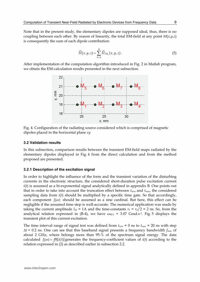
Fig. 4 displays the arbitrary placement representing the set of eight magnetic dipoles in the horizontal plane Oxy considered for the validation of the calculation method under study. To generate the various behaviours of EM-field graphs, the dipole axes are randomly oriented as follows: M1, M4, M5 and M8 along Ox-axis, M2 and M6 along Oy, and M3 and M7 along Oz. These dipoles are in this case, flowed by an ultra-short duration transient current i(t) which is considered as a pulse signal. These elementary dipoles are supposed formed by wire circular loops having radius a = 0.5 mm.

www.intechopen.com


9

Note that in the present study, the elementary dipoles are supposed ideal, thus, there is no coupling between each other. By reason of linearity, the total EM-field at any point M(x,y,z) is consequently the sum of each dipole contribution:

8

1

( , , ) ( , , )kM

k

H x y z H x y z=

=∑iif iif. (5)

After implementation of the computation algorithm introduced in Fig. 2 in Matlab program,

we obtain the EM-calculation results presented in the next subsection.

Fig. 4. Configuration of the radiating source considered which is comprised of magnetic dipoles placed in the horizontal plane xy

3.2 Validation results

In this subsection, comparison results between the transient EM-field maps radiated by the elementary dipoles displayed in Fig. 4 from the direct calculation and from the method

proposed are presented.

3.2.1 Description of the excitation signal

In order to highlight the influence of the form and the transient variation of the disturbing currents in the electronic structure, the considered short-duration pulse excitation current i(t) is assumed as a bi-exponential signal analytically defined in appendix B. One points out that in order to take into account the truncation effect between tmin and tmax, the considered sampling data from i(t) should be multiplied by a specific time gate. So that accordingly, each component ( )I ω should be assumed as a sine cardinal. But here, this effect can be negligible if the assumed time step is well-accurate. The numerical application was made by taking the current amplitude IM = 1A and the time-constants τ1 = τ2/2 = 2 ns. So, from the analytical relation expressed in (B-4), we have ω95% ≈ 3.07 Grad.s-1. Fig. 5 displays the transient plot of this current excitation.

The time interval range of signal test was defined from tmin = 0 ns to tmax = 20 ns with step ∆t = 0.2 ns. One can see that this baseband signal presents a frequency bandwidth fmax of about 2 GHz, where belongs more than 95-% of the spectrum signal energy. The data calculated ( ) [ ( )]I fft i tω = generates the frequency-coefficient values of i(t) according to the relation expressed in (2) as described earlier in subsection 2.2.

www.intechopen.com


10

3.2.2 Discussions on the computed results

By considering the set of eight magnetic dipoles presented in Fig. 4 which are excited by the

same pulse current plotted in Fig. 5 yields the H-field component (Hx, Hy and Hz) mappings

depicted in Fig. 6 at the arbitrary time t0 = 2 ns and in the horizontal plane parallel to (Oxy)

referenced z0 = 6.5 mm above the radiating source.

Fig. 5. Transient plot of the considered excitation current i(t)

Fig. 6. Maps of H-field components detected at the height z0 = 6.5 mm above the radiating

source: (a) Hx, (b) Hy and (c) Hz obtained from the direct calculation

www.intechopen.com


11

This height was arbitrarily chosen in order to generate a significant NF effect in the

considered frequency range. The dimensions of the mapping plane were set at Lx = 110 mm

and Ly = 100 mm with space-resolution equal to ∆x = ∆y = 2 mm. First, by using the

harmonic expressions of the magnetic field components, the maps of the frequency-

dependent H-field are obtained from fmin = 0.05 GHz to fmax = 2.50 GHz with step ∆f = 0.05

GHz. Fig. 7 represents the corresponding mappings of the H-field component magnitudes at

f0 = 2 GHz.

Fig. 7. Maps of H-field components magnitude obtained at the frequency f0 = 2 GHz: (a) Hx,

(b) Hy and (c) Hz directly calculated from expressions (A-8), (A-9) and (A-10)

After the Matlab program implementation of the algorithm indicated by the flow chart

schematized in Fig. 2, the results shown in Figs. 8(a)-(d) are obtained via the combination of

the frequency-dependent data of the H-field components associated to the frequency-

coefficients of the excitation signal plotted in Fig. 5. One can see that the EM-maps

presenting the same behaviors as those obtained via the direct calculations displayed in Fig.

6 were established. In addition, we compare also as illustrated in Fig. 9 the modulus of the

H-fields from the method under study and from the 3D EM Field Simulator - CST

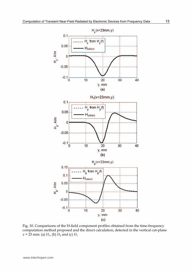
(Computer Simulation Technology). Furthermore, as evidenced by Figs. 10(a)-(c), very good

correlation between the profiles of the H-field components detected in the vertical cut-plane

along Oy and localized at x = 23 mm was observed. To get further insight about the time-

dependent representation of the H-field components, curves showing the variations of Hx(t),

Hy(t) and Hz(t) at the arbitrary point chosen of the mapping plane having coordinates (x = 19

mm, y = 35 mm) are plotted in Figs. 11(a)-(c).

www.intechopen.com


12

As results, once again, we can find that the H-field components from the frequency data fit

very well the direct calculated ones. As aforementioned, due to the truncation effects, the

Hx-component presents a slight divergence at the ending time of the signal. This is

particularly due to the numerical noises at the very low value of the EM field as the case of

the x-component which is absolutely twenty times less than the two other components.

In order to prove in more realistic way the relevance of the investigated method, one

proposes to treat the radiation of concrete electronic devices in the next section.

Fig. 8. Maps of H-field components calculated from the time-frequency computation method

proposed for z0 = 6.5 mm: (a) Hx, (b) Hy, (c) Hz

Fig. 9. Comparison of H-field maps modulus |H|(t0 = 2 ns) obtained from the direct

formulae (in left) and from the time-frequency computation method proposed for

z0 = 6.5 mm

www.intechopen.com


13

Fig. 10. Comparisons of the H-field component profiles obtained from the time-frequency computation method proposed and the direct calculation, detected in the vertical cut-plane x = 23 mm: (a) Hx, (b) Hy and (c) Hz

www.intechopen.com


14

Fig. 11. Comparisons of the H-field components temporal variation obtained from the time-frequency computation method proposed and the direct calculation, detected in the arbitrary point (x = 19 mm, y = 35 mm): (a) Hx, (b) Hy and (c) Hz

www.intechopen.com


15

4. Application with the Transient NF emitted by a microstrip device proof-of-concept

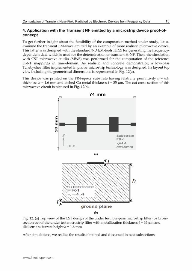
To get further insight about the feasibility of the computation method under study, let us examine the transient EM-wave emitted by an example of more realistic microwave device. This latter was designed with the standard 3-D EM-tools HFSS for generating the frequency-dependent data which is used for the determination of transient H-NF. Then, the simulation with CST microwave studio (MWS) was performed for the computation of the reference H-NF mappings in time-domain. As realistic and concrete demonstrator, a low-pass Tchebychev filter implemented in planar microstrip technology was designed. Its layout top view including the geometrical dimensions is represented in Fig. 12(a).

This device was printed on the FR4-epoxy substrate having relativity permittivity εr = 4.4, thickness h = 1.6 mm and etched Cu-metal thickness t = 35 µm. The cut cross section of this microwave circuit is pictured in Fig. 12(b).

(a)

(b)

Fig. 12. (a) Top view of the CST design of the under test low-pass microstrip filter (b) Cross-section cut of the under test microstrip filter with metallization thickness t = 35 µm and dielectric substrate height h = 1.6 mm

After simulations, we realize the results obtained and discussed in next subsections.

www.intechopen.com


16

4.1 CST-computation results

The low-pass filter under test was simulated with CST MWS in the time interval range

delimited by tmin = 0 ns and tmax = 20 ns with step ∆t = 0.2 ns. Therefore, the magnetic-field

maps are presented in Fig. 13. These curves are recorded at the arbitrary instant time t0 = 2

ns. Note that this structure was excited by the input transient current plotted in Fig. 5. It

results the graphs of H-field components displayed in Fig. 13.

Fig. 13. Maps of transient H-field components detected at t = 2 ns: (a) Hx, (b) Hy and (c) Hz computed from the commercial tool CST

www.intechopen.com


17

Similar to the previous section, these H-field components were mapped in the horizontal

plane placed at the height z0 = 6 mm above the bottom surface of the considered filter and

delimited by -38 mm < x < 38 mm and -24 mm < y < 24 mm with space-step ∆x = ∆y = 2 mm.

By using the frequency-dependent data convoluted with the excitation test signal, we will

present next that we can regenerate these transient H-field maps.

4.2 Analysis of the results obtained from the transient field computation method proposed

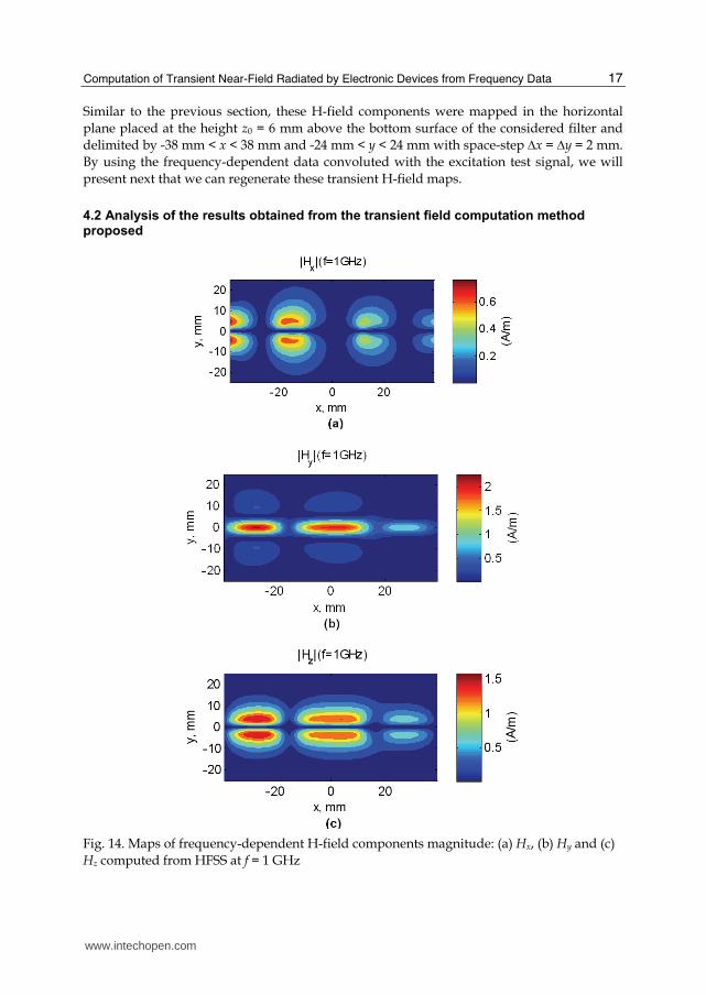
Fig. 14. Maps of frequency-dependent H-field components magnitude: (a) Hx, (b) Hy and (c)

Hz computed from HFSS at f = 1 GHz

www.intechopen.com


18

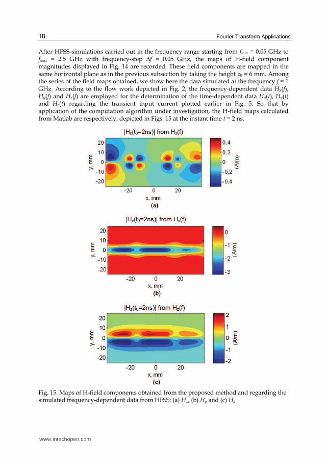
After HFSS-simulations carried out in the frequency range starting from fmin = 0.05 GHz to fmax = 2.5 GHz with frequency-step ∆f = 0.05 GHz, the maps of H-field component magnitudes displayed in Fig. 14 are recorded. These field components are mapped in the same horizontal plane as in the previous subsection by taking the height z0 = 6 mm. Among the series of the field maps obtained, we show here the data simulated at the frequency f = 1 GHz. According to the flow work depicted in Fig. 2, the frequency-dependent data Hx(f), Hy(f) and Hz(f) are employed for the determination of the time-dependent data Hx(t), Hy(t) and Hz(t) regarding the transient input current plotted earlier in Fig. 5. So that by application of the computation algorithm under investigation, the H-field maps calculated from Matlab are respectively, depicted in Figs. 15 at the instant time t = 2 ns.

Fig. 15. Maps of H-field components obtained from the proposed method and regarding the simulated frequency-dependent data from HFSS: (a) Hx, (b) Hy and (c) Hz

www.intechopen.com


19

Despite the slight difference of Hx-maps, we observe that the maps are perfectly well-

correlated to those introduced in Fig. 13 of subsection 4.1. For the further smart illustration

of the results correlation, comparisons of H-field profiles calculated with the method

proposed (grey curves) and those from CST (black curves) for x = -5 mm are plotted Fig. 16.

Fig. 16. Comparisons between Oy-profiles of the H-field components computed with CST

software and those obtained from the proposed method

The imperfection of the results presented here are due to the numerical errors mainly caused

by the solver and the meshing inaccuracies. Note that one evaluates relative errors of about

10 % for |Hx|, |Hy| and |Hz|. Despite the apparent difference between the results from the

method under investigation and the commercial EM-tool CST-computations, once again,

very good correlations between the profiles of the H-field components are realized by

considering the data recorded in the vertical cut-plane equated by x = -5 mm as explained in

Fig. 16.

In nutshell, the computation results exposed in this paper reveal the effectiveness and the

operability of the method developed for the case of elementary magnetic dipoles and also by

considering the NF EM-radiation of realistic use case electronic devices.

5. Concluding remarks

A computation method of transient NF EM-field radiated by electronic devices excited by a

complex wave or ultra-short duration transient signal is stated in this chapter. In addition to

the evanescent wave integration, the originality of the NF calculation method developed lies

on the consideration of the radiation deeming the UWB structures which is literally from DC

to microwave frequency ranges. It is based on the convolution of the frequency-dependent

www.intechopen.com


20

EM-wave data with a transient excitation pulse current. A methodological analysis was made by taking into account a complex waveform of the transient pulse signal exciting the radiation source structure considered. It was explained how the frequency-bandwidth of the frequency-dependent baseband EM-field must be chosen according to the excitation current considered.

In order to demonstrate the relevance of the method investigated, it was first, implemented into Matlab program and then, applied to the determination of the H-field radiated by a microwave circuit in UWB. As consequence, the feasibility of the method was verified with two types of structures. First, with the semi-analytical calculation implemented in Matlab by considering the frequency- and time-dependent expressions of the magnetic NF radiated by a set of magnetic dipoles, an excellent agreement with the results from the calculation method developed were found. Then, further more practical analysis was performed with the determination of transient H-NF from the frequency-dependent data computed with a standard commercial 3-D EM-tool. For this second test, the H-NF emitted by a low-pass planar microstrip filter was treated. For both cases, the excitation current injected to the structures was assumed as an ultra-short transient pulse having half-bandwidth lower than 5 ns which presents a baseband frequency spectrum with bandwidth of about 2.5 GHz from DC. With the examples of complex structures tested, very good agreement between the transient H-field component maps and profiles was realized from the method proposed and those directly calculated from the well-known standard tools and from classical mathematical EM-formulae.

It is interesting to point up that the NF computation method introduced in this chapter is advantageous in terms of:

1. Simplicity of the EM-field maps determination for any waveform of transient excitation even with ultra-short duration which is very hard to simulate with most of commercial simulation tools. The method developed can be used for the determination of the NF maps in time-domain which is practically very difficult to measure in the realistic contexts.

2. It is flexible for various types of excitation signals which can be expressed analytically and also from the realistic use case of disturbing signal generally met in EMC area (Wiles 2003, Liu, K. 2011, Hubing 2011).

3. It can be adapted also to different forms of electrical and electronic structures for low- and high-frequency applications. Globally speaking, it offers a possibility to work in UWB from DC to unlimited upper frequency limit.

4. One can achieve significant EM-field measurement in very short time-duration with base band measured data in wide bandwidth.

However, its main drawback is the limitation in term of time step which depends on the frequency range of the initial frequency-data considered and also the necessity of powerful computer for the achievement of high accurate results.

In the next step of this work, we plane to extend this method to transpose in time-domain the modelling of EM-radiation with the optimized association of elementary dipoles (Vives-Gilabert et al. 2009, Fernández-López et al. 2009). Then, we are hopeful that the method developed in this chapter is very helpful for EMC/EMI investigations of modern electrical/electronic systems as the case of hybrid vehicle embedded circuits (Vye 2011,

www.intechopen.com


21

Tröscher 2011, Kopp 2011) where the transient NF effects are susceptible to disturb the system functioning.

6. Appendix

This appendix contains two parts of theoretical parts concerning the transient NF radiated by the elementary magnetic dipoles (Baum 1971 & 1976, Singaraju & Baum 1976, Ravelo et al. 2011a & 2011b, Lui Y. et al. 2011a & 2011b) and the bi-exponential signal processing.

6.1 Appendix A: Analytical study of the magnetic dipole radiation in time-domain

By definition, the magnetic dipole moment of the elementary circular loop shown earlier in Fig. 3 (see section 3) is written as:

( , ) ( ) ( ) zMp r t p t r uδ= ⋅ ⋅f f

, (A-1)

with r is the distance between the dipole centre and the point M(r,θ,φ) as shown in Fig. 3. By analogy with the definition of the time-variant vector established by Hertz in 1892 (Hertz 1892), the H-field components in the spherical coordinate system:

( , , , ) ( , , , ) ( , , , )rrH H r t u H r t u H r t uθ ϕθ ϕθ ϕ θ ϕ θ ϕ= + +iif f f f, (A-2)

are expressed as:

2

( ) ( )cos( ) 1( , , , )

2r

p pH r t

r v tr

τ τθθ ϕ π∂⎡ ⎤= +⎢ ⎥∂⎣ ⎦ , (A-3)

2

2 2 2

( ) ( ) ( )sin( ) 1( , , , )

4

p p prH r t

r v tr v tθ τ τ τθθ ϕ π

⎡ ⎤∂ ∂= + +⎢ ⎥∂ ∂⎢ ⎥⎣ ⎦ , (A-4)

( , , , ) 0H r tϕ θ ϕ = , (A-5)

where v is the wave-velocity, and τ is the time delayed variable which is defined as /t r vτ = − . One underlines that the magnetic dipole is also an Hertzian dipole so that

( , ) / 0i r t r∂ ∂ = . In the frequency domain, the spherical coordinate of the H-field component formulas radiated by the magnetic dipole pictured in Fig. 3 which is supposed flowed by an harmonic current with amplitude IM denoted:

2( ) j ft j tM MI f I e I eπ ω− −= = , (A-6)

are written as (Balanis 2005):

( )2

3( , , , ) 1 cos( )

2

jkrMr

I aH r f jkr e

rθ ϕ θ −= + , (A-8)

2

2 23

sin( )( , , , ) (1 )

4

jkrMI aH r f jkr k r e

rθ θθ ϕ −= + − , (A-9)

www.intechopen.com


22

( , , , ) 0H r fϕ θ ϕ = , (A-10)

where j is the complex number 1− and the real 2 /k f vπ= expresses the wave number at

the considered frequency f. Then, through the classical relationship between the spherical

and cartesian coordinate systems, one can determine easily the expressions of the

components Hx, Hy and Hz.

6.2 Appendix B: Spectrum analysis of bi-exponential signal

A bi-exponential form signal with parameters τ1 and τ2 is analytically expressed as:

1 2/ /( ) ( )t tMi t I e eτ τ− −= − . (B-1)

The analytical Fourier transform expression of this current is written as:

1 2

1 2

( ) ( )1 1

MI Ij j

τ τω ωτ ωτ= −+ + , (B-2)

with ω is the angular frequency. This yields the signal frequency spectrum formulation

expressed as:

1 2

2 2 2 21 2

( )(1 )(1 )

MI Iτ τω τ ω τ ω

−= + + . (B-3)

To achieve at least 95-% of excitation signal spectrum energy, the frequency-data should be

recorded in baseband frequency range with angular frequency bandwidth equal to:

2 2 2 2 2 2 21 2 1 2 1 2

95%1 2

( ) 1600

2

τ τ τ τ τ τω τ τ− + − −= . (B-4)

7. Acknowledgment

Acknowledgement is made to EU (European Union) and Upper Normandy region for the

support of these researches. These works have been implemented within the frame of the

“Time Domain Electromagnetic Characterisation and Simulation for EMC” (TECS) project

No 4081 which is part-funded by the Upper Normandy Region and the ERDF via the

Franco-British Interreg IVA programme.

8. References

Adada, M. (2007). High-Frequency Simulation Technologies-Focused on Specific High-

Frequency Design Applications. Microwave Engineering Europe, (Jun. 2007), pp. 16-

17

Agilent EEsof EDA. (2008). Overview: Electromagnetic Design System (EMDS), (Sep. 2008)

[Online]. Available from:

http://www.agilent.com/find/eesof-emds

www.intechopen.com


23

Ansoft corporation. (2006). Simulation Software: High-performance Signal and Power Integrity,

Internal Report

ANSYS, (2009). Unparalleled Advancements in Signal- and Power-Integrity, Electromagnetic

Compatibility Testing, (Jun. 16 2009) [Online]. Available from:

http://investors.ansys.com/

Archambeault, B.; Brench, C. & Connor, S. (2010). Review of Printed-Circuit-Board Level

EMI/EMC Issues and Tools. IEEE Trans. EMC, (May 2010), Vol. 52, No.2, pp. 455-

461, ISSN 0018-9375

Balanis, C. A. (2005). Antenna Theory: Analysis and Design, in Wiley, (3rd Ed.), 207–208, New

York, USA, ISBN: 978-0-471-66782-7

Barriere, P.-A.; Laurin, J.-J. & Goussard, Y. (2009). Mapping of Equivalent Currents on High-

Speed Digital Printed Circuit Boards Based on Near-Field Measurements. IEEE

Trans. EMC, (Aug. 2009), Vol.51, No.3, pp. 649 - 658, ISSN 0018-9375

Baudry, D.; Arcambal, C.; Louis, A.; Mazari, B. & Eudeline, P. (2007). Applications of the

Near-Field Techniques in EMC Investigations. IEEE Trans. EMC, (Aug. 2007),

Vol.49, No.3, pp. 485-493, ISSN 0018-9375

Baum, C. E. (1971). Some Characteristics of Electric and Magnetic Dipole Antennas for Radiating

Transient Pulses, Sensor and Simulation Note 405, 23 Jan. 71

Baum, C. E. (1976). Emerging Technology for Transient and Broad-Band Analysis and

Synthesis of Antennas and Scaterrers, Interaction Note 300, Proceedings of IEEE,

(Nov. 1976), pp. 1598-1616

Braun, S.; Gülten, E.; Frech, A. & Russer, P. (2009). Automated Measurement of Intermittent

Signals using a Time-Domain EMI Measurement System, Proceedings of IEEE Int.

Symp. EMC, pp. 232-235, ISBN 978-1-4244-4266-9, Austin, Texas (USA), Aug. 17-21

2009

Chew, W. C. & Kong, J. A. (1981). Electromagnetic field of a dipole on a two-layer earth.

Geophysics, (Mar. 1981), Vol. 46, No. 3, pp. 309-315

Cicchetti, R. (1991). Transient Analysis of Radiated Field from Electric Dipoles and

Microstrip Lines. IEEE Trans. Ant. Prop., (Jul. 1991), Vol.39, No.7, pp. 910-918, ISSN

0018-926X

Edwards, R. S.; Marvin, A. C. & Porter, S. J. (2010). Uncertainty Analyses in the Finite-

Difference Time-Domain Method. IEEE Trans. EMC, (Feb. 2010), Vol.52, No.1, pp.

155-163, ISSN 0018-9375

Fernández-López, P.; Arcambal, C.; Baudry, D.; Verdeyme, S. & Mazari, B. (2009). Radiation

Modeling and Electromagnetic Simulation of an Active Circuit, Proceedings of EMC

Compo 09, Toulouse, France, Nov. 17-19 2009

Hertz, H. R. (1892). Untersuchungen ueber die Ausbreitung der Elektrischen Kraft (in

German). Johann Ambrosius Barth, Leipzig, Germany, ISBN-10: 1142281167/ISBN-

13: 978-1142281168

Hubing, T. (2011). Ensuring the Electromagnetic Compatibility of Safety Critical

Automotive Systems. Invited Plenary Speaker at the 2011 APEMC, Jeju, South-

Korea, May 2011

Jauregui, R.; Pous, M.; Fernández, M. & Silva, F. (2010). Transient Perturbation Analysis in

Digital Radio, Proceedings of IEEE Int. Symp. EMC, pp. 263-268, ISBN 978-1-4244-

6307-7, Fort Lauderdale, Florida (USA), Jul. 25-30 2010

www.intechopen.com


24

Jauregui, R.; Riu, P. I. & Silva, F. (2010). Transient FDTD Simulation Validation, Proceedings

of IEEE Int. Symp. EMC, pp. 257-262, ISBN 978-1-4244-6305-3, Fort Lauderdale,

Florida (USA), Jul. 25-30 2010

Jun-Hong, W.; Lang, J. & Shui-Sheng, J. (1997). Optimization of the Dipole Shapes for

Maximum Peak Values of the Radiating Pulse, Proceedings of IEEE Tran. Ant. Prop.

Society Int. Symp., Vol.1, pp. 526-529, Montreal, Que., Canada, 13-18 Jul 1997, ISBN

0-7803-4178-3

Kopp, M. (2011). Automotive EMI/EMC Simulation. Microwave Journal, (Jul. 2011), Vol.54,

No.7, pp. 24-32

Lakhtakiaa, A.; Varadana, V. K. & Varadana, V. V. (1987). Time-Harmonic and Time-

Dependent Radiation by Bifractal Dipole Arrays. Int. J. Electronics, (Dec. 1987),

Vol.63, No.6, pp. 819-824, DOI:10.1080/00207218708939187

Liu, K. (2011). An Update on Automotive EMC Testing. Microwave Journal, (Jul. 2011),

Vol.54, No.7, pp. 40-46

Liu, L.; Cui, X. & Qi, L.. (2009). Simulation of Electromagnetic Transients of the Bus Bar in

Substation by the Time-Domain Finite-Element Method. IEEE Trans. EMC, (Nov.

2009), Vol.51, No.4, pp. 1017-1025, ISSN 0018-9375

Liu, Y.; Ravelo, B.; Jastrzebski, A. K. & Ben Hadj Slama, J. (2011). Calculation of the

Time Domain z-Component of the EM-Near-Field from the x- and y-

Components, Accepted for communication in EuMC 2011, Manchester, UK, Oct. 9-

14 2011

Liu, Y.; Ravelo, B.; Jastrzebski, A. K. & Ben Hadj Slama, J. (2011). Computational

Method of Extraction of the 3D E-Field from the 2D H-Near-Field using PWS

Transform, Accepted for communication in EMC Europe 2011, York, UK, Sep. 26-30

2011

North East Systems Associates (NESA), (2010). RJ45 Interconnect Signal Integrity, (2010 CST

Computer Simulation Technology AG.) [Online]. Available from:

http://www.cst.com/Content/Applications/Article/Article.aspx?id=243

Ordas, T.; Lisart, M.; Sicard, E.; Maurine, P. & Torres, L. (2009). Near-Field Mapping

System to Scan in Time Domain the Magnetic Emissions of Integrated Circuits, Proceedings of PATMOS’ 08: Int. Workshop on Power and Timing Modeling

Optimization and Simulation, Ver. 1-11, Lisbon, Portugal, Sep. 10-12 2008, ISBN

978-3-540-95947-2

Rammal, R.; Lalande, M.; Martinod, E.; Feix, N.; Jouvet, M.; Andrieu, J. & Jecko, B. (2009).

Far Field Reconstruction from Transient Near-Field Measurement Using

Cylindrical Modal Development, Int. J. Ant. Prop., Hindawi, Vol. 2009, Article ID

798473, 7 pages, doi:10.1155/2009/798473

Ravelo, B. (2010). E-Field Extraction from H-Near-Field in Time-Domain by using PWS

Method. PIER B Journal, Vol.25, pp. 171-189, doi:10.2528

Ravelo, B.; Liu, Y.; Louis, A. & Jastrzebski, A. K. (2011). Study of high-frequency

electromagnetic transients radiated by electric dipoles in near-field. IET Microw.

Antennas Propag., (Apr. 2011), Vol. 5, No, 6, pp 692 - 698, ISSN 1751-8725

Ravelo, B.; Liu, Y. & Slama, J. B. H. (2011). Time-Domain Planar Near-Field/Near-Field

Transforms with PWS Method. Eur. Phys. J. Appl. Phys. (EPJAP), (Feb. 2011), Vol.53,

No.1, 30701-pp. 1-8, doi: 10.1051/epjap/2011100447

www.intechopen.com


25

Rioult, J.; Seetharamdoo, D. & Heddebaut, M. (2009). Novel Electromagnetic Field

Measuring Instrument with Real-Time Visualization, Proceedings of IEEE Int.

Symp. EMC, pp. 133-138, ISBN 978-1-4244-4266-9, Austin, Texas (USA), Aug. 17-

21 2009

Schantz, H. G. (2001). Electromagnetic Energy around Hertzian Dipoles. IEEE Tran. Ant.

Prop. Magazine, (Apr. 2001), Vol.43, No.2, pp. 50-62, ISBN 9780470688625

Selin, V. I. (2001). Asymptotics of the Electromagnetic Field Generated by a Point Source in a

Layered Medium. Computational Mathematics and Mathematical Physics, Vol.41, No.6,

pp. 915-939, ISSN 0965-5425

Shi, J.; Cracraft, M. A.; Zhang J. & DuBroff, R. E. (1989). Using Near-Field Scanning to

Predict Radiated Fields, Proceedings of IEEE Ant. Prop. Int. Symp., Vol.3, pp. 1477-

1480, San Jose, CA (USA)

Singaraju, B. K. & Baum, C. E. (1976). A Simple Technique for Obtaining the Near Fields of

Electric Dipole Antennas from Their Far Fields, Sensor and Simulation Note 213, Mar.

76

Smagin, S. I. & Mazalov, V. N. (2005). Calculation of the Electromagnetic Fields of Dipole

Sources in Layered Media. Doklady Physics, (Apr. 2005), Vol.50, No.4, pp. 178-183,

DOI:10.1134/1.1922556

Song, J. & Chen, K.-M. (1993). Propagation of EM Pulses Excited by an Electric Dipole in a

Conducting Medium. IEEE Tran. Ant. Prop., (Oct. 1993), Vol.41, No.10, pp. 1414-

1421, ISSN 0018-926X

Song, Z.; Donglin, S.; Duval, F.; Louis, A. & Fei, D. (2010). A Novel Electromagnetic

Radiated Emission Source Identification Methodology. Proceedings of Asia-Pacific

Symposium on EMC, Pekin (China), Apr. 12-16 2010, ISBN 978-1-4244-5621-5

Sten, J. C.-E. & Hujanen, A. (2006). Aspects on the Phase Delay and Phase Velocity in the

Electromagnetic Near-Field. PIER Journal, Vol. 56, pp. 67-80, doi:10.2528

Tröscher, M. (2011). 3D EMC/EMI Simulation of Automotive Multimedia Systems.

Microwave Journal, (Jul. 2011), Vol.54, No.7, pp. 34-38

Vives-Gilabert, Y.; Arcambal, C.; Louis, A.; Daran, F.; Eudeline, P. & Mazari, B. (2007).

Modeling Magnetic Radiations of Electronic Circuits using Near-Field Scanning

Method. IEEE Tran. EMC, (May 2007), Vol.49, No.2, pp. 391-400, ISSN 0018-

9375

Vives-Gilabert, Y.; Arcambal, C.; Louis, A.; Eudeline, P. & Mazari, B. (2009). Modeling

Magnetic Emissions Combining Image Processing and an Optimization Algorithm.

IEEE Tran. EMC, (Nov. 2009), Vol.51, No.4, pp. 909-918, ISSN 0018-9375

Vye, D. (2011). EMI by the Dashboard Light. Microwave Journal, (Jul. 2011), Vol.54, No.7, pp.

20-23

Wiles, M. (2003). An Overview of Automotive EMC Testing Facilities, Proceedings of

Automotive EMC Conf. 2003, Milton Keynes, UK, Nov. 6 2003

Winter, W. & Herbrig, M. (2009). Time Domain Measurement in Automotive Applications,

Proceedings of IEEE Int. Symp. EMC, pp. 109-115, ISBN 9781424442669, Austin, Texas

(USA), Aug. 17-21 2009

Xie, L. & Lei, Y. (2009). Transient Response of a Multiconductor Transmission Line With

Nonlinear Terminations Excited by an Electric Dipole. IEEE Trans. EMC, (Aug.

2009), Vol.51, No.3, pp. 805-810, ISSN 0018-9375

www.intechopen.com


26

Yang, T.; Bayram, Y. & Volakis, J. L. (2010). Hybrid Analysis of Electromagnetic Interference

Effects on Microwave Active Circuits Within Cavity Enclosures. IEEE Trans. EMC,

(Aug. 2010), Vol.52, No.3, pp. 745-748, ISSN 0018-9375

www.intechopen.com

Fourier Transform ApplicationsEdited by Dr Salih Salih

ISBN 978-953-51-0518-3Hard cover, 300 pagesPublisher InTechPublished online 25, April, 2012Published in print edition April, 2012

InTech EuropeUniversity Campus STeP Ri Slavka Krautzeka 83/A 51000 Rijeka, Croatia Phone: +385 (51) 770 447 Fax: +385 (51) 686 166www.intechopen.com

InTech ChinaUnit 405, Office Block, Hotel Equatorial Shanghai No.65, Yan An Road (West), Shanghai, 200040, China

Phone: +86-21-62489820 Fax: +86-21-62489821

The book focuses on Fourier transform applications in electromagnetic field and microwave, medicalapplications, error control coding, methods for option pricing, and Helbert transform application. It is hopedthat this book will provide the background, reference and incentive to encourage further research and resultsin these fields as well as provide tools for practical applications. It provides an applications-oriented analysiswritten primarily for electrical engineers, control engineers, signal processing engineers, medical researchers,and the academic researchers. In addition the graduate students will also find it useful as a reference for theirresearch activities.

How to referenceIn order to correctly reference this scholarly work, feel free to copy and paste the following:

Blaise Ravelo and Yang Liu (2012). Computation of Transient Near-Field Radiated by Electronic Devices fromFrequency Data, Fourier Transform Applications, Dr Salih Salih (Ed.), ISBN: 978-953-51-0518-3, InTech,Available from: http://www.intechopen.com/books/fourier-transform-applications/computation-of-transient-near-field-radiated-by-electronic-devices-from-frequency-data

computation of transient near-field radiated by electronic...

Documents