computation of rate and volume of stream depletion … · puting rate and volume of stream...

Techniques of Water-Resources Investigations

of the United States Geological Survey

Chapter D1

COMPUTATION OF RATE AND VOLUME OF

STREAM DEPLETION BY WELLS

By C. T. Jenkins

Book 4

HYDROLOGIC ANALYSIS AND INTERPRETATION

http://www.usgs.gov/

reidell

Click here to return to USGS Publications

../index.html

UNITED STATES DEPARTMENT OF THE INTERIOR

CECIL D. ANDRUS, Secretary

GEOLOGICAL SURVEY

V. E. McKelvey, Director

First printing 1968

Second printing 1969

Third printing 1977

UNITED STATES GOVERNMENT PRINTING OFFICE, WASHINGTON : 1968

For sale by the Branch of Distribution, U.S. Geological Survey, 1200 South Eads Street, Arlington, VA 22202

PREFACE

The series of manuals on techniques describes procedures for planning and executing specialized work in water-resources investigations. The material is grouped under major subject headings called books and further subdivided into sections and chapters; Section D of Book 4 is on inter- related phases of the hydrologic cycle.

The unit of publication, the chapter, is limited to a narrow-field of subject matter. This format permits flexibility in revision and publication as the need arises.

Provisional drafts of chapters are distributed to field offices of the U.S. Geological Survey for their use. These drafts are subject to revision because of experience in use or because of advancement in knowledge, techniques, or equipment. After the technique described in a chapter is sufficiently developed, the chapter is published and is sold by the U.S. Geological Survey, 1200 South Eads Street, Arlington, VA 22202 (author- ized agent of Superintendent of Documents, Government Printing Office).

This manual is an expanded version of a paper, “Techniques for computing rate and volume of stream depletion of wells” (Jenkins, 1968a), that was prepared in the Colorado District, Water Resources Division, in cooperation with the Colorado Water Conservation Board and the South- eastern Colorado Water Conservancy District and published in Ground Water, the journal of the Technical Division, National Water Well Asso- ciation.

III

CONTENTS

Page

Preface- _ _ _ _ _ _ _ _ _ _ _ _ _ _ - - - - - - - - - - - - - - - - - _ _ III Abstract------ ____________________________ 1 Introduction___---------------------------- 1 Definitions and assumptions _____ _ _ _ _ _- ______ 2 Descriptions of curves and tables _____________ 3

Effects during pumping- _ _ _ _ _ _ _ _ _ _ _ _ _ _ _ _ 3 Residualeffects----- _______________ -__- 4

Intermittent pumping _______________ 5

Sample computations- - _ _ _ _ _ _ _ ___ __ _ _ _ _ _ _ _ _ _ Mathematical bases for curves and tables-.. _ _ _ _

Definitions- _ _ ___- ______ ______________ _ Mathematical base for curve A---- - ______ Mathematical base for curve B ___________

References-------- ____________________ -___

Page

8 16 16 16 16 17

FIGURES

1. Curves to determine rate and volume of stream depletion _____ _ _ _ __ _ _ _ __ _ _ _ __ _- 2. Curves to determine rate of stream depletion during and after pumping- _ _ _ _ _ __ _ 3. Curves to determine volume of stream depletion during and after pumping- _ _ __ _ 4. Example of residual effects of well pumping 35 days- _ ____________ -_- ____ _____ 5. Curves showing the effects of intermittent and steady pumping on a stream- _ _ _ _

TABLES

1. Values of q/Q, &, and Qsdf -!- corresponding to selected values of t/&f _____--------

2. Computation of residual effects of pumping- ____________ - __________________ 3. Computation of the effects of two selected patterns of pumping on a nearby

stream____--________________________________________-______-_--_-------

6 7 7

10

Page

5

6

8 V

COMPUTATION OF RATE AND VOLUME OF STREAM DEPLETION BY WELLS

By C. T. Jenkins

Abstract

When field conditions approach certain assumed conditions, the depletion in flow of a nearby stream caused by pumping a well can be calculated readily by using dimensionless curves and tables. Computa- tions can be made of (1) the rate of stream depletion at any time during the pumping period or the following nonpumping period, (2) the volume of water induced from the stream during any period, pumping or nonpumping, and (3) the effects, both in rate and volume of stream depletion, of any selected pattern of intermittent pumping. Sample computations illustrate the use of the curves and tables. An example shows that intermittent pumping may have a pattern of stream depletion not greatly different from a pattern for steady pumping of an equal volume.

The residual effects of pumping, that is, effects after pumping stops, on streamflow may often be greater than the effects during the pumping period. Adequate advance planning that includes consideration of residual effects thus is essential to effective management of a stream-aquifer system.

Introduction

With increasing frequency, problems of water management require evaluation of effects of ground-water withdrawal on surface supplies. Both rate and volume effects have significance. Effects after the pumping stops (called residual effects in this paper) are important also but have not previously been examined in detail. In fact, residual effects can be much greater than those during pumping. Curves and tables shown in this paper, although applicable to a large range of interactions, are especially oriented to the solution of problems involving very small interactions and to the evaluation of residual effects. Where many wells are concentrated near a stream, the combined withdrawals can have a significant effect on the availability of water in the stream.

In some instances, especially in the evaluation of residual effects, the grid spacing on the

charts shown may prove to be too coarse to provide the desired precision. However, this precision can be attained either by interpolating between the tabular values supplied or by using curves prepared by plotting the tabular values on commercially available chart paper that is more finely divided.

The relations between the pumping of a well and the resulting depletion of a nearby stream have been derived by several investigators (Theis, 1941; Conover, 1954; Glover and Balmer, 1954; Glover, 1960; Theis and Conover, 1963; Hantush, 1964, 1965). The relations generally are shown in the form of equations and charts; however, except for the charts shown by Glover (1960), which were in a publication that had limited distribution, the charts are useful as computational tools only in the range of comparatively large effects, and rather formidable equations must be solved to evaluate small effects. The average user retreats in dismay when faced by the mysticism of “line source integral, ” “complementary error function,” or “the second repeated integral of the error function.” The primary purpose of this report is to provide tools that will simplify the seemingly intricate computations and to give examples of their use.

Because this writer definitely is a member of the community of “average users,” he has exercised what he believes to be his prerogative of reversing the usual order of presentation. In this paper, the working tools-curves, tables, and sample computations-are shown first, and the discussion of their mathematical bases is relegated to the end of the report. The usefulness of the tools will not be greatly enhanced by an understanding of the material at the end of the report; it is shown for the benefit of those who desire to examine the mathematical bases of the tools.

1

2 TECHNIQUES OF WATER-RESOURCES INVESTIGATIONS

The techniques demonstrated in this paper are not new, but they seem to have been rather well concealed from most users in the past. Their value to water managers is apparent, especially in the estimation of total volume of depletion and of residual effects.

Virtually all the literature that discusses the effects of pumping on streamflow fails to mention that the effects of recharge are identical, except for direction of flow. (See Glover, 1964, p. 48.) Only pumping will be considered in this paper, but the reader should be aware that the terms “recharging” and “accretion” can be substituted for “pumping” and “depletion,” respectively.

Definitions and Assumptions

To avoid confusion owing to the use of the same symbol for the dimension time as for transmissivity, symbols for the dimensions time and length are set in Roman type, are capi- talized, and are enclosed in brackets. All other symbols, except that designating the mathematical term “second repeated integral,” are set in italics.

Stream depletion means either direct depletion of the stream or reduction of ground-water

flow to the stream. The symbols used in the main body of the

report are defined below (those that have to do only with the mathematical bases are defined at the end of the report in the section on this subject) :

T = transmissivi ty, [L2/T] ; S= the specific yield of the aquifer,

dimensionless; t-rtime, during the pumping period,

since pumping began, [T] ; t,= total time of pumping, [T] ; tf= time after pumping stops, [T]; &=the net steady pumping rate, [L3/T];

the steady pumping rate less the rate at which pumped water returns to the aquifer;

Q= the rate of depletion of the stream, [L3/Tl ;

&t=the net volume pumped during time t, b”l;

&t,=the net volume pumped, [L3]; v= the volume of stream depletion dur-

ing time t, tp, or tp+tl, ]L3];

a= the perpendicular distance from the pumped well to the stream, [L];

sdj=the stream depletion factor, [T]. The term “stream depletion factor” was

introduced by Jenkins (1968a). It is arbitrarily defined as the time coordinate of the point where v=28 percent of Qt on a curve relating v and t. If the system meets the assumptions listed in this section, sdj=a2S/T; in a complex system it can be considered to be an effective value of a2S/T. The value of the sdj at any location in the system depends upon the integrated effects of the following: Irregular impermeable boundaries, stream meanders, aquifer properties and their area1 variation, distance from the stream, and imperfect hydraulic connection between the stream and the aquifer.

The curves and tables in this report are dimensionless and can be used with any units. The units in the system must be consistent, however. For example, if & and p are in acre-feet per day (acre-ft/day), v must be in acre-feet (acre-ft). If a is in feet (ft) and T/S is in gallons per day per foot (gal/day-ft), the value of T/S must be converted to square feet per day (ft2/day). A T/S value of 10 6gal/day-ft equals (lO”gal/day-ft) X (lft3/7.48 gal) equals 134,000 ft2/day.

The assumptions made for this analysis are the same as other investigators have made and are as follows: 1. T does not change with time. Thus for a

water-table aquifer, drawdown is considered to be negligible when compared to the saturated thickness.

2. The temperature of the stream is assumed to be constant and to be the same as the temperature of the water in the aquifer.

3. The aquifer is isotropic, homogeneous, and semi-infinite in area1 extent.

4. The stream that forms a boundary is straight and fully penetrates the aquifer.

5. Water is released instantaneously from storage.

6. The well is open to the full saturated thickness of the aquifer.

7. The pumping rate is steady during any period of pumping.

Field conditions never meet fully the idealized conditions described by the above assumptions.

COMPUTATION OF RATE AND VOLUME OF STREAM DEPLETION BY WELLS 3

0 The usefulness of the t,ools presented in this report will depend to a large extent on the degree to which the user recognizes departures from ideal conditions, and on how well he under- stands the effects of these departures on stream depletion.

Departure from idealized conditions may cause actual stream depletions to be either greater or less than the values determined by methods presented in this report. Although the user usually cannot determine the magnitude of these discrepancies, he should, where possible, be aware of the direction the discrepancies take.

Jenkins (196813) has described the use of a model to evalute t,he effects on stream depletion of certain departures from the ideal. If a model is not available, the user of this report can be guided in estimating the sdf by the effects calculated in that report for selected departures from the idealized system. Intuitive reasoning will be useful in estimating the effects of departures from the ideal that are difficult to in- corporate in a model. For example, where drawdowns at the well site are a substantial

0

proportion of the aquifer thickness, T will decrease significantly. A decrease in T results in a decrease in the amount of stream depletion relative to the amount of water pumped.

Variations in water temperatures will cause variations in stream depletion, especially by large-capacity wells near the stream. Warm &ater is less viscous than cold water; hence stream depletion will be somewhat greater in the summer than in the winter, given the same pattern of pumping. Stream stages affect water- table gradients, and hence stream depletion.

Lowering of the water table on a flood plain may result in the capture of substantial amounts of water that would otherwise be transpired. The effect is similar to intercepting another recharge boundary, and the proportion of stream depletion to pumpage is decreased. Interception of a valley wall or other negative boundary will have the opposite effect.

If large-capacity wells are placed close to a stream, and streambed permeability is low compared to aquifer permeability, the water table may be drawn down below the bottom of the streambed. (See Moore and Jenkins, 1966.)

0 Under these conditions, stream depletion de-

pends upon streambed permeability, area of the streambed, temperature of the water, and stage of the stream, and the methods presented in this report are not applicable.

Both during and after pumping, some part and at times all of stream depletion can consist of ground water intercepted before reaching the stream. Thus a stream can be depleted over a certain reach, yet still be a gaining stream over that reach. The flow at the lower end of the reach is less than it would have been had depletion not occurred, and less by the amount of depletion. In order to predict the amount of streamflow at the lower end of the reach, residual effects of previous pumping or recharge must be considered. They can be approximately accounted for by using past records of pumping and recharge to “prestress” the calculations. The depletion due to the pumping under consideration will then be superimposed on the residual depletion, and the resultant value will be the net direct depletion from the stream.

Description OF Curves and Tables

Effects during pumping

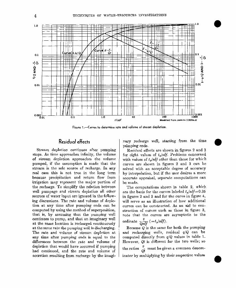
Curves A and B in figure 1 apply during the period of steady pumping. Curve A shows the relation between the dimensionless term t/sdf and the rate of stream depletion, p, at time t,

expressed as a ratio to the pumping rate Q. Curve B shows the relation between t/scJf and the volume of stream depletion, w, during time t, expressed as a ratio to the volume pumped,

Qt. The two curves labeled 1 -Q/Q and 1 - & are

shown to facilitate determination of values of

Q/Q and & when the ratios exceed 0.5. The

coordinates of curves A and B are tabulated in table 1. The number of significant figures shown for the values in table 1 was determined by needs for some of the computations described in the next section. Precision to more than two significant figures in reporting results probably will never be warranted.


0.001 0.1 1 .o 10 100 1000

t/sdf ModlIned from Jenkins (1%8a.b)

Figure I .- Curves to determine rate and volume of stream depletion.

Residual effects

Stream depletion continues after pumping stops. As time approaches infinity, the volume of stream depletion approaches the volume pumped, if the assumption is made that the stream is the sole source of recharge. In any real case this is not true in the long term because precipitation and return flow from irrigation may represent the major portion of the recharge. To simplify the relation between well pumpage and stream depletion all other sources of water input are ignored in the following discussions. The rate and volume of depletion at any time after pumping ends can be computed by using the method of superposition, that is, by assuming that the pumping well continues to pump, and that an imaginary well at the same location is recharged continuously at the same rate the pumping well is discharging. The rate and volume of stream depletion at any time after pumping ends is equal to the differences between the rate and volume of depletion that would have occurred if pumping had continued, and the rate and volume of accretion resulting from recharge by the imagi-

nary rechaxge well, starting from the time ptimping ends.

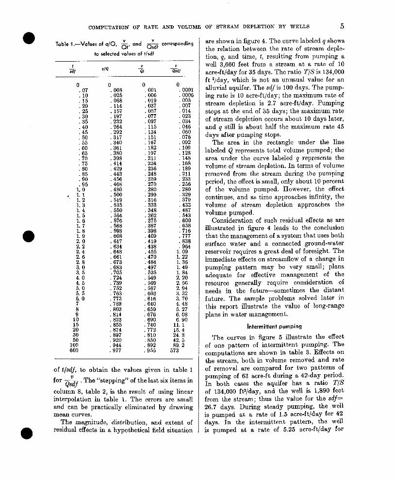
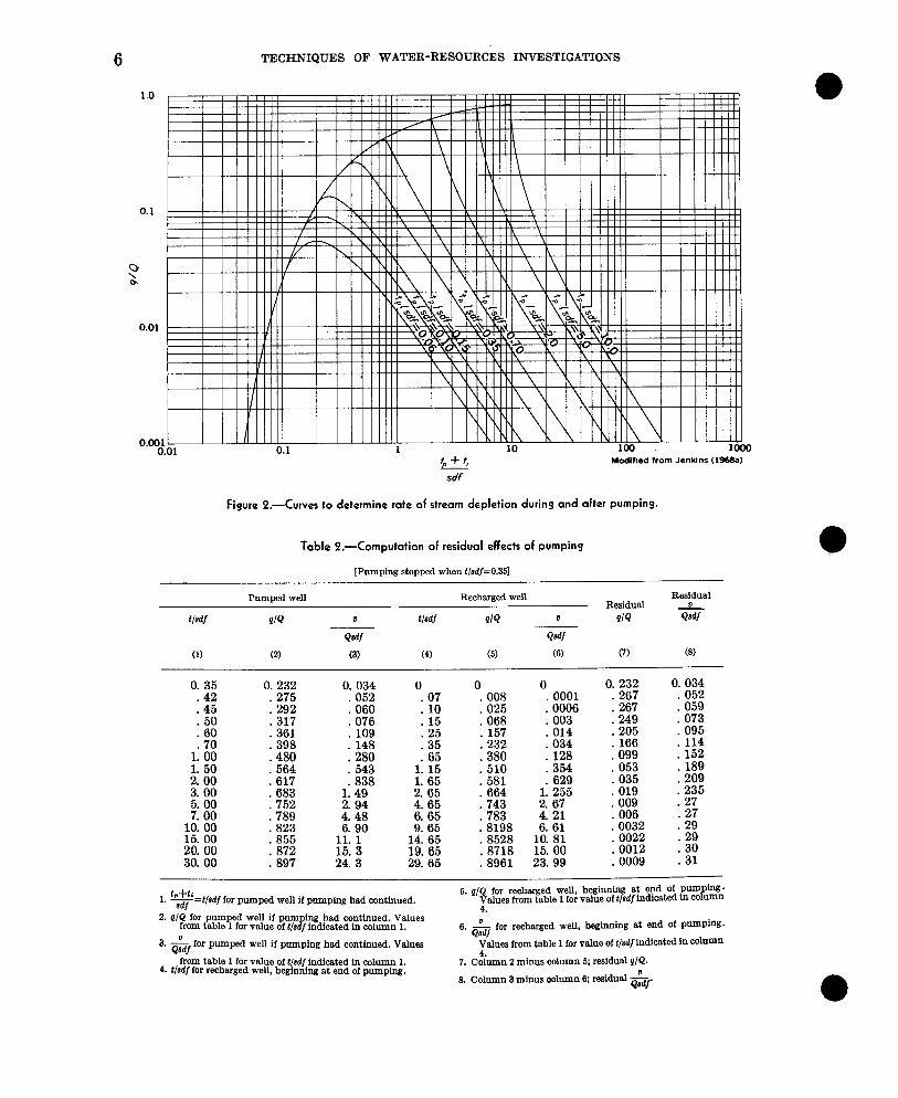
Residual effects are shown in figures 2 and 3 for eight values of tPlsdj. Problems concerned with values of tp/sdj other than those for whit h curves are shown in figures 2 and 3 can be solved with an acceptable degree of accuracy by interpolation, but if the user desires a more accurate appraisal, separate computations can be made.

The computations shown in table 2, which are the basis for the curves labeled t,/scZj=0.35 in figures 2 and 3 and for the curve in figure 4, will serve as an illustration of how additional curves can be constructed. As an aid to con- struction of curves such as those in figure 3, note that the curves are asymptotic to the

ordinate & ( = t,/sdf> .

Because-Q-is the same for both the pumping and recharging wells, residual n/Q can be computed directly from a/Q values in table 1. However, Qt is different for the two wells; SO

the ratios 2 must be given a common denom- Qt

inator by multiplying by their respective values


Table 1 .-Values of q/O, &, and & corresponding

to selected values of t/sdf

0 .008 .025 .068 .114 .157 .197 .232 .264 .292 .317 .340 .361 .380 . 398 .414 .429 443

:456 .468 .480 .500 .519 .535 .550 . 564 576

:588 . 598 .608 .617 .634 .648 .661 .673 .683 .705 .724 .739 .752

: 777633 . 789 .803

. E

.855

.874

. 897

.920 * 944 .977

0 .OOl .006 .019 ,037 .057 .077 .097 .115

. E':

.167

.182

. 197

.211

.224

.236

.248

. 259

.270

.280

.299

.316

. 333

.348

.362

.375

.387

.398

.409

.419

.438

: :;o" .484 .497 . 525 . 549 . 569 .587 .603 .616 .640 . 659 .676 . 690 .740 .772 .810 .850 . 892 . 955

0 .OOOl .0006 .003 .007 .014 .023 .034 .046 .060 .076 . 092 .109 .128 .148 .168 .189 .211 .233 .256 .280 . 329 .379 .433 .487 .543 600

:658 .716 .777 .838 964

1: 09 1. 22 1. 36 1. 49 1. 84 2. 20 2. 50 2. 94 3. 32 3. 70 4. 48 5. 27 6. 08 6. 90

11. 1 15. 4 24. 3 42. 5 89. 2

573

of tlsdf, to obtain the values given in table 1

- for QsY7y * The “stepping” of the last six items in

column 8, table 2, is the result of using linear interpolation in table 1. The errors are small and can be practically eliminated by drawing mean curves.

The magnitude, distribution, and extent of residual effects in a hypothetical field situation

are shown in figure 4. The curve labeled p shows the relation between the rate of stream depletion, p, and time, t, resulting from pumping a well 3,660 feet from a stream at a rate of 10 acre-ft/day for 35 days. The ratio T/S is 134,000 ft 2/day, which is not an unusual value for an alluvial aquifer. The sdj is 100 days. The pumping rate is 10 acre-ft/day; the maximum rate of stream depletion is 2.7 acre-ft/day. Pumping stops at the end of 35 days; the maximum rate of stream depletion occurs about 10 days later, and p still is about half the maximum rate 45 days after pumping stops.

The area in the rectangle under the line labeled Q represents total volume pumped; the area under the curve labeled p represents the volume of stream depletion. In terms of volume removed from the stream during the pumping period, the effect is small, only about 10 percent of the volume pumped. However, the effect continues, and as time approaches infinity, the volume of stream depletion approaches the volume pumped.

Consideration of such residual effects as are illustrated in figure 4 leads to the conclusion that the management of a system that uses both surface water and a connected ground-water reservoir requires a great deal of foresight. The immediate effects on streamflow of a change in pumping pattern may be very small; plans adequate for effective management of the resource generally require consideration of needs in the future-sometimes the distant future. The sample problems solved later in this report illustrate the value of long-range plans in water management.

Intermittent pumping

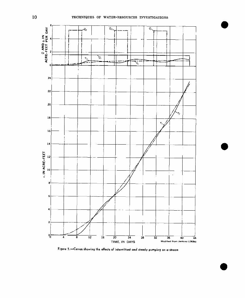
The curves in figure 5 illustrate the effect of one pattern of intermittent pumping. The computations are shown in table 3. Effects on the stream, both in volume removed and rate of removal are compared for two patterns of pumping of 63 acre-ft during a 4%day period. In both cases the aquifer has a ratio T{S of 134,000 ft?/day, and the well is 1,890 feet from the stream; thus the value for the sdj= 26.7 days. During steady pumping, the well is pumped at a rate of 1.5 acre-ft/day for 42 days. In the intermittent pattern, the well is pumped at a rate of 5.25 acre-ft/day for


G sdf

Modified from Jenkins W66a)

Figure I.- Curves to determine rate of stream depletion during and after pumping.

Table I.-Computation of residual effects of pumping

[Pumping stopped when t/sd/=0.351

Pumped well Recharged well Residual Residual v

t/M

(1)

g/Q

(2)

u

QW

(3)

t/M

(4)

916

(5)

”

Qsdf

03

dQ

(7)

QM

(8)

0. 35 0. 232 0. 034 0

.t; . . 275 292 .052 060

. Z8 1317 : 076

.07 . 10

. 15 : 361 : 109 .25

.70 398 148 .35 1. 00 .480 .280 65 1. 50 2. 00 5:;

1: 15

3. 00 : 683 : xii 1. 65

1. 49 2. 65

10: EX 00

. 752 2. 94 4. 65

.789 . 823 4. 6. 48 90 9. 6. 65 65 15. 00 855 11. 1 14. 65 20. 00 : 872 15. 3 19. 65 30.00 .897 24. 3 29. 65

0 . 008 . 025 . 068 . 157 .232 .380 . 510 . 581 . 664 . 743 .783 . 8198 . 8528 . 8718 . 8961

0 0.232 “: % . 059 . 073

014 . . % . 354

1: t:; 035

: 019 .209 .235

2. 67 .009 .27 4. 21 . 006 .27 6. 61 . 0032 . 29

10. 81 15. 00 : CK);; . 3;

23. 99 . 0009 . 31

1. F=t/sdflor pumped well if pumping had continued.

2. g/Q for pumped well if pmn ing had continued. Values from table 1 for value of t/s 8. fmdtcated in column 1.

3. -!- for pumped well if pumping had continued. Values QW

from table 1 for value of t/adj indicated in column 1. 4. tlsdffor recharged well, beginning at end of pumping.

5. g/Q for recharged well, beginnin at end Of pUmPfW. plues from table 1 for value oft f sdf mdlcated ~II OOl~n

6. QG, for recharged well, beginning at end of pumping. Values from table 1 for value of tlsdfindicated in 0011DIn

7. C&mn 2 minus column 5; residual g/Q.

3. Column 3 minus column 6; residual 2. 4W


0.0001 0.01 1

t, sdf

10 100 1000 M0doN.d from hnkins (l%BW

Figure 3.-C urves to determine volume of stream depletion during and after pumping.

0 Figure 4.-E xample of residual effects of well pumping 35 days. I

4 days beginning 5 days after the beginning of the period, shut down 10 days, pumped 4 days, shut down 10 days, pumped 4 days, and shut down 5 days. The computed effects of the pattern of intermittent pumping are compared in figure 5 with those of the steady rate. The comparisons indicate that, within quite large ranges of intermittency, the effects of intermittent pumping are approximately the same as those of steady, continuous pumping of the same volume.

8 TECHNIQUE$ OF WATER-RESOURCES INVESTIGATIONS

Table 3.-Computation of the effects of two selected 0

[a=l,&@ft, T/S=l34,1XMft2/day, adf=26.7 days. Intermittent pumping rate=5.25ecre-ft/dsy,

Time from beginning of period (days)

Steady pumping Intermittent pumping

Pumping period (lst42d day inclusive) Pumping period (6th-9th day inclusive)

tr (I (scrLft)

Time v t/W q/Q

zz (acre-ft (days) Wf q/Q

per day) Bsdf

0 0 0 0 0 ___-___________-___-----

. 187 122.1 102 . 006 . 15 0 0

-3.17 .031 .33 1:; 4” . 150 . 068 -_. ---

.449 . 060 .44 . 712 : zt 153 .60 2 ;’

:E :471 446 .262 : 216 :76: 1:: 1. 236 . 525 . 398 . 79 15: 9 1. 386 . 548 . 479 . 82 19. 2 1. 573 . 573 . 585 . 86 23. 4

7 .262 . 127 :;: : 524 674 : 061 080

$i 1: 787 049 .050 .034

i; 1.199 1. 386 . . 029 023

-_ .-----. 0

. 003

. 015

. 044

.054

. 061

. 071

. 074

. 081

Sample C omputations

To illustrate the use of the curves and tables, solutions are shown of problems that might arise in the conjunctive management of ground water and surface water.

Problem I

Management criteria require that pumping cease when the rate of stream depletion by pumping reaches 0.14 acre-ft/day: 1. Under this restriction how long can a well

1.58 miles from the stream be pumped at the rate of 2 acre-ft/day if T/S is lo6 gal/ day-ft, and what is the volume of stream depletion during this time?

2. If pumping this well is stopped when q=O.l4 acre-ft/day, what will the rate of stream depletion be 30 days later? What will be the volume of stream depletion at that time?

3. What will be the largest rate of stream depletion and when will it occur?

Given :

p= 0.14 acre-f t/day &= 2 acre-f t/day a= 1.58 miles T/S= lo6 gal/day-f t ti=30 days

&+&3jT=a2= (1.58 mi)2 (5,280 ft/mi)2 T/S (lPgal/day-ft) (1 ft3/7.48gal)

=520 days.

Find :

t, v at t, p at t, + tt w at t, + tt p max t of p max.

Part 1 From information given, the ratio of the

rate of stream depletion to the rate of pumping is

(0.14 acre-ft/day)EO o7 n/Q=,, acre-ft/day) ’ ’

From curve A (fig. 1)

t/saj=0.15.

Substitute the value under “Given” for sdf, and

t= (0.15) (520 days) =78 days.

The total time the well can be pumped is 78 days.

When t/sdf=0.15.

then from curve B (fig. l),

&=0.02.

Substitute the values for & and t, and the volume of stream depletion during this time is

v= (0.02) (2 acre-ft/day) (78 days) =3.1 acre-ft.

COMPUTATION OF RATE AND VOLUME OF STREAM DEPLETION BY WELLS

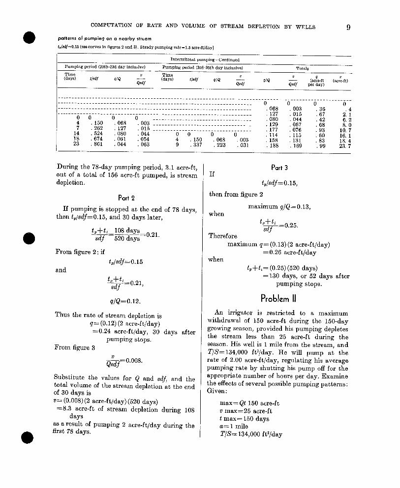
patterns of pumping on a nearby strtam

9

t,/adf=0.15 (see curves in figures 2 and 3). Steady pumping rate=l.5 acre-ft/day]

I Intermittent mmmine-Contimmd

Pumping period (20th-23d day inclusive)

Time u (days) tlW q/Q

Gi

- _I~ Pumping period (32d-35th day inclusive)

Time (days)

0 WJ q/Q

Qddr 916

Totals

0

G (ac!e-It

per day) (ackft)

__________________-_____________________------------------------------------------------------------- ____-_______________----------------------------------------------- 0 0 0 0 _________________-______________________--------------------------- . 068 . 003 . 36 ________________________________________---------------------------

: 0 0 0

. 127 . 015 . 67 2: ‘:

150 . 068 __________________________________ 080 . 044 . 42

7 : 262 . 127 . 003 -_________________________________ : 129 .057 . 68 .

524 080 015 __________________________________ .177 .076 .93

ii: i

044 :: : 674 : 061 : 054 :

0 10. 7

0 0 114 . 115 .60

23 . 861 . 044 . 063 150 . 068 . 003 : 158

16. 1

9 : 337 . 223 . 031 131 83

. 188 : 169 ‘. 99 18. 4 23. 7

During the 7%day pumping period, 3.1 acre-ft, out of a total of 156 acre-ft pumped, is stream depletion.

Part 2 If pumping is stopped at the end of 78 days,

then t,/sdf=0.15, and 30 days later,

tP+tdEds;ys-O 21

sdf 520 days * *

From figure 2: if t,/sdf=0.15

and t,+ti

sdf =0.21,

q/&=0.12.

Thus the rate of stream depletion is p= (0.12) (2 acre-ft/day) =0.24 acre-ft/day, 30 days after

pumping stops. From figure 3

-- Q;df-o.oo8.

Substitute the values for Q and sdf, and the total volume of the stream depletion at the end of 30 days is ZJ= (0.008) (2 acre-ft/day) (520 days) =8.3 acre-ft of stream depletion during 108

days as a result of pumping 2 acre-ftjday during the first 78 days.

Part 3 If

t,/sdf=cm,

then from figure 2

maximum q/&=0.13, when

tp+ti p-=0.25. sdf

Therefore maximum q= (0.13) (2 acre-ft/day)

=0.26 acre-ft/day when

t,+t,=(0.25)(520 days) =130 days, or 52 days after

pumping stops.

Problem II

An irrigator is restricted to a maximum withdrawal of 150 acre-ft during the 150-day growing season, provided his pumping depletes the stream less than 25 acre-ft during the season. His well is 1 mile from the stream, and T/S=134,000 fV/day. He will pump at the rate of 2.00 acre-ft/day, regulating his average pumping rate by shutting his pump off for the appropriate number of hours per day. Examine the effects of several possible pumping patterns: Given :

max=Qt 150 acre-ft v max=25 acre-ft t max= 150 days a=1 mile T/S= 134,000 ft2/day


6

16 -

TIME, IN DAYS Mod#f8ed from Jenkms (1968e)

Figure 5.-C urves showing the effects of intermittent and steady pumping on a stream


s+a2~,T=??=-@J280 ft)z-=20g days. T/S 134,000 ft2/day

Find : Various pumping patterns possible within

the restrictions given.

Part 1

First, test to see if both restrictions apply to any combination of pumping time and rate within the 150-day period. Try ending pumping the last day of the season, beginning pumping at a time and rate such t,hat pumping 150 acre-ft will result in a depletion of the stream of 25 acre-ft at the end of pumping.

Qt=l50 acre-ft, v=25 acre-ft; 6 =0.167.

From curve B (fig. 1)

Time will be

t=(0.54) (209 days) =113 days, or 37 days after beginning

of season.

Pumping rate will be

Q= 150 acre-ft

113 days =1.33 acre-ft/day.

He can pump 16 hours per day, beginning 113 days before the end of the season.

If pumping 150 acre-ft during the 113-day period at the end of the season results in 25 acre-ft of stream depletion, it follows that pumping 150 acre-ft-regardless of rate-in a shorter period at the end of the season will result in less than 25 acre-ft depletion, and the 150 acre-ft limit will apply. It also follows that pumping 150 acre-ft in the earlier periods will result in more than 25 acre-ft of stream depletion, hence the restriction on stream depletion will apply during the first part of the season.

Part 2

Begin pumping 60 days after the beginning of the season. Test reasoning that the restriction on volume pumped applies.

Qt= 150 acre-ft, t=90 days,

tlsdj= 9O.Pv =0*43. 209 days

From curve B

$=0.13.

The volume of stream depletion is

v=(O.13) (150 acre-ft)=19.5 acre-ft.

The restriction on the volume of stream depletion has not been exceeded; therefore, the restriction on volume pumped does apply, and the allowable pumping rate would be

Q= 150 acre-ft 90 days

= 1.67 acre-ft/day

which is the equivalent of pumping at the rate of 2.00 acre-ft/day for 20 hours per day.

Part 3

Begin pumping at the beginning of the season, pump for 73 days. Test reasoning that the restriction on stream depletion applies.

t,/sdj=73 days/209 days=0.35.

From figure 3, for

and t/sdj=O.35

t,+tc= 150 days sdf 209 days

=0.72,

Gj=o.12.

The steady pumping rate is

25 acre-ft Q= co.12l (20g dajs)=l’OO acre-f t/day,

and the net volume pumped is

Qt= (1.00 acre-ft/day) (73 days)=73 acre-ft.

Therefore, the restriction on volume of stream depletion does apply. He can pump 12 hours per day at a rate of 2.00 acre-ftlday during a 73-day pumping period at the beginning of the season.


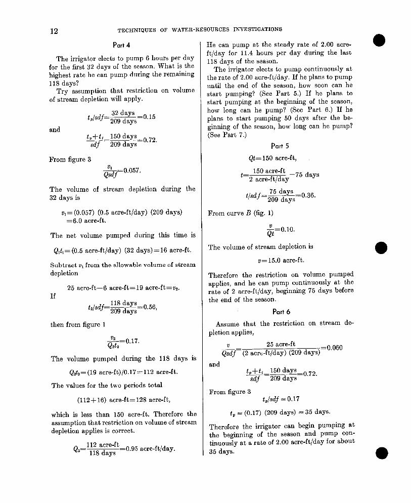
Part 4

The irrigator elects to pump 6 hours per day for the first 32 days of the season. What is the highest rate he can pump during the remaining 118 days?

Try assumption that restriction on volume of stream depletion will apply.

and

tp/sdj= 32 days =0.15 209 days

150 dapEO 72 tn+tt sdf 209 days * *

From figure 3

&j=o.057.

The volume of stream depletion during the 32 days is

vl= (0.057) (0.5 acre-ft/day) (209 days) =6.0 acre-ft.

The net volume pumped during this time is

QItl= (0.5 acre-ft’/day) (32 days)=16 acre-ft.

Subtract ZJ~ from the allowable volume of stream depletion

25 acre-f&6 acre-ft=19 acre-ft=vz. If

tp/sdj= 118 dvs=0 56 209 days ’ ’

then from figure 1

*=0.17. Q&z

The volume pumped during the 118 days is

Q&=(19 acre-ft)/O.17=112 acre-ft.

The values for the two periods total

(112-l-16) acre-ft=128 acre-ft,

which is less than 150 acre-ft. Therefore the assumption that restriction on volume of stream depletion applies is correct.

Q2= 112 acre-ft 118 days

=0.95 acre-ft/day.

He can pump at the steady rate of 2.00 acre- ft/day for 11.4 hours per day during the last 118 days of the season.

The irrigator elects to pump continuously at the rate of 2.00 acre-ft/day. If he plans to pump until the end of the season, how soon can he start pumping? (See Fart 5.) If he plans to start pumping at the beginning of the season, how long can he pump? (See Part 6.) If he plans to start pumping 50 days after the beginning of the season, how long can he pump? (See Part 7.)

Part 5

&t=150 acre-ft,

t= 150 acre-ft 2 acre-ft/day

=75 days

t/sd j= 75 days cO.36. 209 days

From curve B (fig. 1)

Z=O.lO. Qt


v= 15.0 acre-ft.

Therefore the restriction on volume pumped applies, and he can pump continuously at the rate of 2 acre-ft/day, beginning 75 days before the end of the season.

Part 6

Assume that the restriction on stream depletion applies,

V 25 acre-ft mj= (2 acre-ft/day) (209 days)

=0.060

and tn+ti-

s&f 150 days=-, 72 209 days . ’

From figure 3 tPfsaj = 0.17

t, = (0.17) (209 days) = 35 days.

Therefore the irrigator can begin pumping at the beginning of the season and pump continuously at a rate of 2.00 acre-ft/day for about 35 days.


Part 7 The net is

Restriction on volume pumped limits pumping time to

150 acre-ft 2 acre&/day

=75 days.

Test to see if depletion restriction would be exceeded by 75 days of pumping beginning 50 days after the beginning of the season.

t,+&=(150-50) days=100 days. If

t,+ti sdf

100 days o 48 =--= 209 days *

and t,/sdj=75 days.1209 days=0.36,

then from figure 3

Gj=0.72.


D= (0.72)(2 acre-ft/day) (209 days)

~30 acre-ft,

which exceeds the 25 acre-ft restriction. Try stopping pumping after 69 days. Use

values from table 1 instead of interpolation between curves in figure 3.

&=(lOO-69) days=31 days. If

t,+tt df

=0.48, then sj=0.070,

and if

t,=0.15, then A-=0.003. sdf QW

The net is

Gj=0.067.

The volume of steam depletion is

v=28 acre-ft.

Try t,=54 days, ti=46 days,

and

t”+t”,o.48, - W

Q;;j=o.070,

t* -=0.22, -- sdf

Qrdj-0.010.

Gj=0.060.


v=25 acre-ft.

Therefore, the irrigator can pump continuously at a rate of 2 acre-ft/day during the 54-day period beginning 50 days after the season begins.

Problem III

A well 4,000 feet from the stream is shut down after pumping at a rate of 250 gallmin for 150 days; T/S=67,000 ft2/day. 1. What effect did pumping the well have on the

stream during the pumping period? 2. What will be the effect during the next 216

days after pumping was stopped? 3. What would the effect have been if pumping

had continued during the entire 366 days? Given :

Q =250 gal/min t, = 150 days, 366 days tt =216 days a =4,000 feet T/S= 67,000 ft2/day

sdj= (4000 ft)”

67.000 ft2/dav =239 days.

Find: ’ ’ ” p and v for t,= 150 days p and v for t,+t,=366 days p and v for t,=366 days

Part 1

t,/sdj=150 days/239 days=0.63.

The rate of pumping in consistent units is

When =l.l acre-ft/day.

t/sdj=O.63. From curve A

q/Q= 0.37.


From curve B

-21_=0.19. Qt

At the end of 150 days,

q=(l.l acre-ft/day) (0.37) =0.41 acre-ft/day,

v=(l.l acre-ft/day) (150 days) (0.19) =31 acre-ft.

Part 2

When t,+t,=(150+216) days=366 days,

t +ti L-=1.53. W

From figure 2 by interpolation,

n/&=0.11.

From figure 3 by interpolation,

Gj=o.33.

Thus, 216 days after pumping ceased,

q= (0.11) (1.1 acre-ft/day) =O.12 acre-ft/day,

v= (0.33) (1.1 acre-ft/day) (239 days) =87 acre-ft.

The additional volume of stream depletion during the 216-day period would be

(87-31) acre-ft=56 acre-ft.

Part 3

If pumping had continued for the entire 366-day period,

t -=1.53, sdf

and from trible 1, n/&=0.568 and

x=0.366. Qt

q= (0.568) (1.1 acre-ft/day) =0.62 acre-ft/day,

v= (0.366) (1 .l acre-ft/day) (366 days) = 147 acre-ft.

During the last, 216 days the stream depletion would have been

v=(147-31) acre-ft=116 acre-ft.

Problem IV

A municipal well is to be drilled in an alluvial aquifer near a stream. Downstream water uses require that depletion of the stream be limited to no more than 5,000 cubic meters during the dry season, which commonly is about 200 days long. The well will be pumped continuously at the rate of 0.03 m3/sec (cubic meters per second) during the dry season only. Wet season recharge is ample to replenish storage depleted by the pumping in the previous dry season, thus residual effects can be disregarded. T=30 cm2/sec (square centimeters per second), s= 0.20.

What, is the minimum allowable distance between the well and the stream?

Given : v=5,000 m3 &=0.03 m”/sec t,=200 days T= 30 cm2/sec s=o.20

Qt= (0.03 m3/sec) (200 days) (86,400 set/day) = 5.184X 105m3

&=5,000 m3/5.184X105 m3=0.01.

Find: a

From curve B

o ,,=(200 days) (86,400 set/day) (30 cm2/sec), a2(0.20)

a,=(200) (86,400) (3O)*=2*l6x 1o’o cm2 (0.12) (0.20) 9

a=l.47X lo5 cm=1,470 meters.

Problem V

A water company wants to install a well near a stream and pump it 90 days during the sum-


mer to supplement reservoir supplies. Down- stream residents have protested that the well might dry up the stream. Natural ,streamflow at the lower end of the reach that would be affected by pumping is not expected to go below 2.0 ft?/sec in most years, and the downstream users have agreed that the well can be installed if depletion of the stream is limited to a maximum of 1.5 ft3/sec. The well would be 500 feet from the the stream and would pump 1,000 gpm. T=50,000 gpd/ft, and S =0.20. 1. Will the rate of stream depletion exceed

1.5 fV/sec during the first season or any following season?

2. If so, when will the rate of stream depletion exceed 1.5 ft3/sec?

3. At what rate could the well be pumped in order not to exceed 1.5 ft3/sec of stream depletion?

Given : p max allowable= 1.5 ft3/sec a=500 feet T=50,000 gal/day-ft s=o.20 Q= 1,000 gal/min

sdjC(500 ft)2(0.20)(7.48 gal/ft3) --- --- -=7.5 days 50,000 gal/day-ft

Find : p max t for q=1.5 ft3/sec Q for p= 1.5 ft3/sec

Part 1

t,=90 days.

tp/8dj= 12. From figure 1,

l--q/&=0.155.

Therefore q/&=0.845,

p=(0.845)(1,000 gal/min)(1,440 min/day) 7.48 gal/ft3

=1.63X105 ft3/day

= 1.88 ft3fsec.

Therefore by the end of the first pumping period, the rate of stream depletion would have exceeded the allowable depletion of 1.5 ft3/sec.

Part 2

p= 1.5 ft3/sec= (1.5 ft3/sec) (86,400 set/day)

=1.30X lo5 ft3/day Q=l,OOO gal/mm

(1,000 gal/mm) (1,440 min day) =------ 7.48 gal/l??

=1.93X105 ft3/day

q/Q= 1.30X105/1.93X 105=0.67

1--q/Q=l.OO-0.67=0.33.

From figure 1, curve 1 -q/Q

t/sdj=2.7,

t= (2.7) (7.5)=20 days.

Therefore, the rate of strea,m depletion will exceed 1.5 ft3/sec after 20 days pumping at 1,000 gal/min.

Part 3

From “Part 1,” p/&=0.845. Q=q/O.845

= (1.30X lo5 ft3/day)/0.845 =1.54x 105 ft3/day = 800 gal/mm

Therefore, if pumping were reduced to 800 gal/ min, the rate of stream depletion would not exceed 1.5 ft3/sec during the first go-day period of pumping.

However, the residual effects of this pumping would carry over through the next pumping period.

The residual effect of the first pumping period on rate of stream depletion at the end of the second period, assuming no pumping during the second period, is as follows:

t,+t,=90 days+365 days=455 days.

-=61, ti/sdj=49. sdf

From figure 1,

(I-qg/Q),+,=O.O73,

(l--q/&),=0.081,

16 TECHXIQUES OF WATER-RESOURCES INVESTIGATIONS

and q/&=0.008.

?erfc x= the second repeated integral of the a

Thus the rate of depletion is

a=(0.008) (1.54X105 fF/day)

= 1,230 ft3/day

=0.014 ft3/sec.

The effects are very slight. Pumping 800 gal/ min during the second pumping period would exceed the allowable stream depletion rate by only 0.014 ft3/sec. Reduction of the pumping rate to about 750 gal/min would keep rate of stream depletion below 1.5 ft3/sec during several successive pumping seasons.

Mathematical Bases for Curves

and Tables

The literature concerning the effect of a pumping well on a nearby stream contains several equations and charts that, although superficially greatly different, yield identical results. The basic curves and table (Curves A and B, and table 1) of this report can be derived from any of the published expressions. A cursory review of some of the pertinent equations may be useful to those interested in the mathematics.

Definitions

The notation that has been used in the literature is even more diverse than the published equations; consequently, definitions of only selected terms are given below. Complete definitions of all terms used are in the indicated references.

erf s=the error function of z

=- ;o s

Ze-i2dt=l -erfc x

erfc x=the complementary error function of x

error function. The line source integral (Maasland and

Bittinger, 1963, p. 84)

In the notation used in the main body of this report,

-J zj

x/J4Pt= 4t

Definitions and tabular values of erf x ,erfc 2, and i*erfc x are shown by Gautschi (1964, p. 297, 310-311, 316-317). Tabular values of the line source integral are shown by Maasland and Bittinger (1963, p. 84) and by Glover (1964, p. 45-53).

Mathematical base for curve A

Curve A and its coordinates in table 1 can be computed ,from Theis (1941), Conover (1954), and Theis and Conover (1963)

S orize-k sed u&,

from Glover and Balmer (1954)

a/Q=1 --P(s,/~~)

from Glover (1960)

(1

(2

> 0

(3)

and from Hantush (1964, 1965)

Q,= Qerfc (U) (4)

Theis transformed his basic integral into equation 1 because the basic integral is laborious to evaluate, but in the form of equation 1, is amenable to either numerical or graphical solution. Equations 2, 3, and 4 are identical, and in the notation used in this paper are

n/Q=erfc(E)=l-erf(#$)- (5)


Mathematical base for curve B References

Curve B and its coordinates in table 1 can be computed either by integration of curve A or of the equations that are the base of curve A. Analytical integration of equations 2 and 3 is shown by Glover (1960) as

Conover, C. S., 1954, Ground-water conditions in the Rincon and Mesilla Valleys and adjacent areas in New Mexico: U.S. Geol. Survey Water-Supply Paper 1230, 200 p. [1955].

Gautschi, Walter, 1964, Error function and Fresnel in- tegrals, in Abramowitz, Milton, and Stegun, I. A., eds., Handbook of mathematical functions with formulas, graphs, and mathematical tables: U.S. Dept. Commerce, Natl. Bur. Standards, Appl. Math. Ser. 55, p. 295-329.

and equation 4 is integrated by Hantush (1964, 1965)

v,= s

‘Q,dt=4Qtoia erfc (U,) 0 (7)

In the notation used in this paper, equation 6 is

and equation 7 is

-11-=4i2erfc df Qt u-1

t *

Equations 8 and 9 both can be expressed in terms extensively tabulated in Gautschi (1964, p. 310-311) as

$=($+l) erfc (.$$)

Before discovering equations 6 and 7, the writer integrated curve A both numerically and graphically. The results were identical, within the limitations of the methods, to those ob- tained from equation 10.

Glover, R. E., 1960, Ground water-surface water rela- tionships [A paper given at Ground Water Section of Western Resources Conference, Boulder, Colo- rado]: Colorado State Univ. paper CER60REG45, 8 pp. [1961].

- 1964, Ground-water movement: U.S. Bur. Rec- lamation Eng. Mon. 31, 67 p.

Glover, R. E., and Balmer, C. G., 1954, River depletion resulting from pumping a well near a river: Am. Geophys. Union Trans., v. 35, pt. 3, p. 468-470.

Hantush, M. S., 1964, Hydraulics of wells, in Chow, Ven te, ed., Advances in Hydroscience, v. 1: New York, Academic Press, p. 386.

- 1965, Wells near streams with semipervious beds: Jour. Geophys. Research, v. 70, no. 12, p. 2829-2838.

Jenkins, C. T., 1968a, Techniques for computing rate and volume of stream depletion by wells: Ground Water, v. 6, no. 2, p. 37-46.

- 1968b, Electric-analog and digital-computer model analysis of stream depletion by wells: Ground Water, v. 6, no. 6, p. 27-34.

Massland, D. E. L., and Bittinger, M. W., eds., 1963, Summaries of solved cases in rectangular coordinates, Appendix A, in Proceedings of the sympo- sium on transient ground water hydraulics: Colorado State Univ. pub. CER63DEM-MWB70, p. 83-84.

Moore, J. E., and Jenkins, C. T., 1966, An evaluation of the effect of groundwater pumpage on the in- filtration rate of a semipervious streambed: Water Resources Research, v. 2, no. 4, p. 691-696.

Theis, C. V., 1941, The effect of a well on the flow of a nearby stream: Am. Geophys. Union Trans., v. 22, pt. 3, p. 734-738.

Theis, C. V., and Conover, C. S., 1963, Chart for determination of the percentage of pumped water being diverted from a stream or drain, in Bentall, Ray, compiler, Shortcuts and special problems in aquifer tests: U.S. Geol. Survey Water-Supply Paper 1545-C pp. C106-Cl09 [1964].

f!? U.S. Government Printing Office: 1977--240~%1/12S