Computation in Cellular Automata:

A Selected Review

Melanie Mitchell

Santa Fe Institute

1399 Hyde Park Road

Santa Fe, NM 87501

U.S.A.

email: mm@santafe.edu

In T. Gramss, S. Bornholdt, M. Gross, M. Mitchell, and T. Pellizzari, Nonstandard Computation,pp. 95–140. Weinheim: VCH Verlagsgesellschaft, 1998.

1 Introduction

Cellular automata (CAs) are decentralized spatially extended systems consisting of large numbersof simple identical components with local connectivity. Such systems have the potential to per-form complex computations with a high degree of efficiency and robustness, as well as to modelthe behavior of complex systems in nature. For these reasons CAs and related architectures havebeen studied extensively in the natural sciences, mathematics, and in computer science. They havebeen used as models of physical and biological phenomena, such as fluid flow, galaxy formation,earthquakes, and biological pattern formation. They have been considered as mathematical objectsabout which formal properties can be proved. They have been used as parallel computing devices,both for the high-speed simulation of scientific models and for computational tasks such as imageprocessing. In addition, CAs have been used as abstract models for studying “emergent” coopera-tive or collective behavior in complex systems. (For collections of papers in all of these areas, see,e.g., Burks, 1970a; Fogelman-Soulie, Robert, and Tchuente, 1987; Farmer, Toffoli, and Wolfram,1984; Forrest, 1990; Gutowitz, 1990; Jesshope, Jossifov, and Wilhelmi, 1994; and Wolfram, 1986.)

In this chapter I will review selected topics related to computation in CAs. The presentation willassume an elementary knowledge of the theory of computation, including formal-language theoryand computability.

A CA consists of two components. The first component is a cellular space1: a lattice of Nidentical finite-state machines (cells), each with an identical pattern of local connections to othercells for input and output, along with boundary conditions if the lattice is finite. Let Σ denote theset of states in a cell’s finite state machine, and k = |Σ| denote the number of states per cell. Each

1CA terminology differs among different authors. The terminology in this chapter will be consistent with mostmodern work.

1

Neighborhood ηPeriodicboundaryconditions

1 010 0 0 001 11t = 0

1 011 1 0 111 11t = 1

Lattice:

Rule table φ: 000 001 010 011 100 101 110 111 0 1 1 1 0 1 1 0

neighborhood:output bit:

Figure 1: Illustration of a one-dimensional, binary-state, r = 1 CA with periodic boundary con-ditions shown iterating for one time step. Wolfram (1983) proposed a numbering scheme forone-dimensional k=2 (“elementary”) CAs in which the output bits are ordered lexicographically, asin the figure, and are read right-to-left (neighborhood 111 first) to form a binary integer between0 and 255. In that scheme, the elementary CA pictured here is number 110.

cell is denoted by an index i and its state at time t is denoted sti (where st

i ∈ Σ). The state sti of

cell i together with the states of the cells to which cell i is connected is called the neighborhood ηti

of cell i.

The second component is a transition rule (or “CA rule”) φ(ηti) that gives the update state s

(t+1)i

for each cell i as a function of ηti .

Typically in a CA a global clock provides an update signal for all cells: at each time step allcells update their states synchronously according to φ(ηt

i).

A one-dimensional, k = 2 (Σ = {0, 1}) CA is illustrated in Figure 1. Here, the neighborhood ofeach cell consists of itself and its two nearest neighbors, and the boundary conditions are periodic(i.e., the leftmost cell is considered to be the right neighbor of the rightmost cell, and vice versa).For one dimensional CAs, the size of the neighborhood ηi (leaving off the t subscript when it isnot needed) is often written as |ηi| = 2r + 1 where r is called the radius of the CA. In the one-dimensional case, φ : Σ2r+1 → Σ. In cases of binary-state CAs where the number of possibleneighborhoods is not too large, the CA rule is often displayed as a lookup table (or rule table)which lists each possible neighborhood together with its output bit, the update value for the stateof the central cell in the neighborhood. The 256 one-dimensional, k = 2, r = 1 CAs are calledelementary CAs (ECAs). The one pictured in Figure 1 is ECA 110, according to Wolfram’s (1983)numbering scheme.

The behavior of CAs is often illustrated using “space-time diagrams” in which the configurationof states in the d-dimensional lattice is plotted as a function of time. (Of course, in most cases space-time diagrams are practical only for d ≤ 2.) Figure 2 gives a space-time diagram of the behavior ofECA 110 on a lattice with N = 200, starting from a randomly generated initial configuration (the

2

0

Time

199

199Site0

Figure 2: A space-time diagram, illustrating the typical behavior of Elementary CA 110. Thelattice, displayed horizontally, starts with a randomly generated initial configuration. Cells in state1 are displayed as black, and cells in state 0 are displayed as white. Time increases down the page.(This and other space-time diagrams given in this chapter were plotted using the lattice automatonsimulation and graphing package la1d, written by James P. Crutchfield.)

lattice is displayed horizontally) and iterated over 200 time steps (with time increasing down thepage).

The ECAs are among the simplest versions of the CA architecture (although, as can be seenin Figure 2, such CAs can give rise to apparently complicated aperiodic behavior). This basicarchitecture can be modified in many ways—increasing the number of dimensions, the number ofstates per cell and the neighborhood size; modifying the boundary conditions; making the CA rulestochastic rather than deterministic; and so on.

CAs are included in the general class of “iterative networks” or “automata networks” (seeFogelman-Soulie, Robert, and Tchuente, 1987 for a review of this general class). CAs are dis-tinguished from other examples of this class in their homogeneous and local connectivity amongcells, homogeneous update rule across all cells, and (typically) relatively small k.

2 Von Neumann’s Self-Reproducing Cellular Automaton

The original concept of cellular automata is most strongly associated with the great scientist andmathematician John von Neumann. According to the history recounted by Burks (1966, 1970b),von Neumann was deeply interested in connections between biology and the (then) new science ofcomputational devices, “automata theory.” Paramount in his mind was the biological phenomenonof self-reproduction, and he had posed a fundamental question: “What kind of logical organizationis sufficient for an automaton to be able to reproduce itself?” The idea of using cellular automataas a framework for answering this question was suggested to von Neumann by Stanislaw Ulam(Burks, 1970b). Thus, the original concept of cellular automata can be credited to Ulam, whileearly development of the concept can be credited to von Neumann.

Von Neumann strongly believed that a general theory of computation in “complex networks of

3

(a) (b)

Figure 3: (a) The von Neumann neighborhood. (b) The Moore neighborhood. In both cases, thecell to be updated is shaded.

automata” such as cellular automata would be essential both for understanding complex systems innature and for designing artificial complex systems. Von Neumann made foundational contributionsto such a theory, and it is thus ironic that the standard model of computation, with a CPU,globally accessible memory, serial processing, and so on has been dubbed the “von Neumann style”architecture, and architectures such as cellular automata have been dubbed “non-von Neumannstyle.”

Von Neumann’s detailed solution to his question, “What kind of logical organization is sufficientfor an automaton to be able to reproduce itself?” was presented in his book Theory of Self-Reproducing Automata (von Neumann, 1966). The manuscript was incomplete at the time of vonNeumann’s death in 1957. The manuscript was edited and completed by Burks, who also givesan excellent detailed overview of von Neumann’s system in Essay 1 of his book Essays on CellularAutomata (Burks, 1970a).

This question has to be framed carefully so that it does not admit trivial solutions (e.g., onecan easily design a CA in which 1s reproduce themselves)—the automaton in question needs tohave a minimal complexity. Von Neumann required that the automaton in question be equivalentin power to a universal Turing machine.

The self-reproducing automaton that von Neumann constructed, here denoted as Mc, is embed-ded in a two-dimensional cellular space with a particular CA rule and a particular initial configu-ration of states. The two-dimensional space is considered to be infinite, and all but a finite numberof cells start out in a special “quiescent” state.

There are 29 possible states per cell (including the quiescent state), and the neighborhood of eachcell consists of five cells: the cell itself and the four bordering cells to the north, south, east, and west(Figure 3a). This two-dimensional neighborhood is now called the “von Neumann neighborhood.”The two dimensional neighborhood consisting of the cell itself and its 8 neighbors (the von Neumannneighborhood plus the diagonal cells) is called the “Moore neighborhood” (Figure 3b).

Figure 4 illustrates schematically the high-level process by which the self-reproducing automatonMc works. Mc consists of a configuration of states which can be grouped into two functional units:a constructing unit, which constructs the new automaton, and a tape unit, which stores and readsthe information needed to construct the new automaton.

The tape unit consists of a tape control and a “tape.” The tape is a linear array of cells thatcontains the information about M , the automaton to be constructed. In particular, it contains (in

4

construction control

tape control . . .

tape

completed part of constructed automaton

uncompleted part ofconstructed automaton

constructing arm

tap

e u

nit

con

stru

ctin

g u

nit

con

stru

ctio

n a

rea

Figure 4: A schematic diagram of the operation of von Neumann’s self-reproducing automaton,illustrating the high-level components. (Adapted from Burks, 1970c.)

left-to-right order) (1) the x and y coordinates (x0, y0) of the lower left-hand corner of the rectanglein which the new automata is to be constructed (the “construction area”); (2) the width α andheight β of that rectangle; and (3) the cell states making up the automaton (listed in reverse orderof where they are to be placed in the rectangle) and a asterisk indicating the end of the tape.

The construction of the new automaton M is carried out by the sending of signals (in the formof propagating cell states) between the tape unit and the constructing unit. The constructing unitconsists of a construction control and a “constructing arm.” As shown in Figure 4, the constructingarm is an array of cells through which cell states to be constructed can be sent from the constructioncontrol to designated places in the construction area.

The original automaton Mc is “turned on” by an external signal sent to the construction control.The construction control then sends a signal to the tape unit, which reads from the tape and sends(via signals) the values of x0, y0, α, and β to the construction control. The construction controlthen causes the construction “arm”—an expanding and contracting array of cell states—to “move”(by changing the states of intermediate cells) from its initial position to the upper left-hand cornerof the construction area. Then the construction control asks for and receives the value of successivestates on the tape, and moves the construction arm to place them in their proper positions in the

5

construction area.

When construction is complete (i.e., the terminating asterisk is read from the tape), the con-struction control moves the construction arm to the lower left-hand corner of M and sends thestart signal to it, which causes M to begin the self-reproduction process anew. Then Mc moves itsconstruction arm back to its original position.

The above is a rough, high-level description of how von Neumann’s self-reproducing automatonworks. Von Neumann’s solution included both this high-level design and its implementation in a29-state cellular automaton. The high-level functions invoked above—reading states from the tape,sending different signals, receiving and recognizing different signals, and so on—are all built up in acomplicated way by primitive CA operations. At the lowest level, von Neumann used primitive CAoperations to synthesize logical operations such as “or,” “and,” and other simple operations suchas delays and signal propagation. These operations were used in turn to synthesize higher-leveloperations such as signal recognizers, the movable construction arm, and so on. Finally, the higher-level operations were used to put together the entire automaton. It is interesting to note that someof the intermediate-level operations were analogous to the primitive elements von Neumann usedin designing the EDVAC—the first “stored program” electronic computer.

It should be clear that Mc is capable of more than self-reproduction—in fact, it can be shownto be a universal constructor, capable of constructing any automaton whose configuration is storedon its tape. (It can also be shown to be capable of universal computation.) Self-reproductionthen reduces to the special case where Mc’s tape contains a description of Mc itself. It is essentialthat the constructed automaton be initially “quiescent” (i.e., its states do not change before itreceives a start signal). If this were not the case, then M might begin a new construction processbefore its own construction is completed, and possibly interfere with its own construction process.Von Neumann’s automaton is initially quiescent; it does not begin its construction process until itreceives an external signal.

Von Neumann insisted that his CA have a reasonably small number of states per cell—otherwisethe question of universal computation and universal construction in a CA could be begged byimplementing high-level capabilities directly in each cell (with a huge number of states). His 29-state construction was later further simplified by Codd (1968) to a CA with eight states per cell,and later by Banks (1971) to four states per cell. Von Neumann’s design itself was implemented ona computer by Pesavento (1996). Langton (1984) studied very simple self-reproducing structuresin CAs in order to understand the minimal requirements for non-trivial self-reproduction.

Other types of self-reproducing automata can be designed—for example, see Hofstadter (1979),Chapter 16, for a discussion of self-reproduction in computer programs and in nature. One com-monality among all such systems is the use of the same information in two modes: first as aninterpreted program that implements a copying engine, and second as uninterpreted data to becopied to form the offspring system. In von Neumann’s system, the initial configuration of statesis interpreted by the CA to implement the copying engine, and also holds the tape containingthe uninterpreted initial configuration of states that will make up the copied automaton M . Thisbasic principle, that the same information is used in these two modes, also forms the basis ofself-reproduction in molecular biology. It is interesting to note that von Neumann’s design of aself-replicating automaton was prior to the discovery of the detailed mechanisms by which DNAreplicates itself.

6

(a)

(b)

cell a cell b

cell h

cell s

P

. . .. . . S-3 -2S -1S 0S 1S 2S 3S

Figure 5: (a) The neighborhood template used in Smith’s universal CA. The cell to be updatedis shaded. (b). A schematic diagram of the operation of Smith’s universal CA. The current cellsimulating the tape head is labeled h, with state P . The cells immediately to its left and right arelabeled a and b, respectively. The cell currently being scanned is labeled s, and has state S0. Theother non-blank tape cells i have states Si. (Adapted from Smith, 1971.)

3 Universal Computation in Cellular Automata

3.1 Smith’s Two-Dimensional Construction

Von Neumann was the first to design a cellular automaton capable of universal computation. Sincethen many others became interested in the problem and either improved on his original constructionor have developed alternative constructions. An early example was Alvy Ray Smith (1971), whoconstructed a series of progressively simpler cellular automata capable of universal computation.The first in the series was a two-dimensional cellular automaton Ms that simulates a given Turingmachine M in “real time”—that is, there is a one-to-one correspondence between the time steps ofMs and the time steps of M .

Smith’s construction is quite straightforward. The main cleverness is using the same CA statesto represent both tape symbols and states of M . Suppose M has m tape symbols (including theblank symbol) and n internal states. In Ms, the number of states per cell k is one plus the maximumof m and n. The cellular space is an infinite two-dimensional space, with all but a finite number of

7

Cell c Neighborhood of c Next state of c conditions

s P p S0 = u

S−1 S∗

0 S1 P = v

0 0 0

h 0 00 P ∗ 0 in all cases

S−1 S0 S1

a 0 0 if X = R

0 0∗ P q if X = L

S−2 S−1 S0

b 0 q if X = R

P 0∗ 0 0 if X = L

S0 S1 S2

Table 1: Part of the transition rule for Smith’s universal CA, given schematically. A Turing machinemove is represented as (u, v) = pXq: scan the current tape symbol u in state v, write a new tapesymbol p and go into state q, and move X, where X is either L (a left move) or R (a right move). Astarred symbol represents the state of cell c, the cell to be updated. (Adapted from Smith, 1971.)

cells being in a “quiescent” state, denoted by 0. A cell neighborhood consists of 7 cells, with theneighborhood template given in Figure 5a. Without loss of generality, assume that n < m. Thenk = m + 1 (where the (m + 1)st state is 0).

The CA works as illustrated in Figure 5b. One row of the space is used to simulate M ’s tape.At each time step t the cells in this row are in states corresponding to the symbols Si on M ’s tapeat time step t in M ’s operation. At any time, all but a finite number of M ’s tape squares areblank. Ms needs to know the extent of this finite tape area, so the leftmost and rightmost cells ofthe finite tape are set to M ’s blank symbol (here called “1”). All other cells outside the currentfinite tape area are set to the quiescent state 0.

The row of cells above the tape row contains one cell that simulates the tape head (labeled h,containing state P ). It is directly above the cell (labeled s) whose symbol S0 is to be scanned attime t. Two other cells are necessary to label: cells a and b, the cells directly to the left and rightof cell h. All cells except the tape cells and h are in the quiescent state.

The actions of M—scan the current tape symbol u in state v, write a new tape symbol p andgo into state q, and move either left or right—can be written in the form (u, v) = pXq, where Xis either L (a left move) or R (a right move). These actions are encoded in Ms’s transition rule,part of which is schematically given in Table 1. (This table leaves out some details, such as entriesdealing with the ends of the finite tape area; see Smith, 1971 for all details.) The starred symbolin each neighborhood configuration is the symbol to be updated by that transition. For example,the first entry in the table is for the scanned cell s. Assuming its value is u, the tape head’s valueis v, and M has the action (u, v) = pXq, s is assigned the new state p. Likewise, the second entryspecifies that the tape head moves by updating the current tape head cell to state 0.

In this way, Ms simulates any given Turing machine M in real time. As a corollary, a CA Us canbe constructed in this way to simulate a universal Turing machine U in real time. (For example,

8

Minsky (1967) described a 6-state, 6-symbol universal Turing machine, so a two-dimensional, 7-state CA can be constructed that simulates it in real time.) In his paper, Smith gives severalother variations of the original construction with different number of states, different neighborhoodtemplates, and one-dimensional architectures.

It should be noted that this approach to universal computation in CAs differs from von Neu-mann’s in that Smith’s construction simulates a particular Turing machine M—a different con-struction is needed for each different Turing machine—whereas von Neumann’s construction cansimulate any Turing machine by setting up the initial configuration in the correct way. Von Neu-mann’s construction, on the other hand, does not simulate Turing machines in anything like realtime.

Many alternative schemes for simulating Turing machines in cellular automata have been for-mulated over the years. For example, Lindgren and Nordahl (1990) constructed an r = 1, k = 7one-dimensional CA in which tape symbols were represented by stationary cell states (as in Smith’sconstruction) but in which the tape head (with internal state) was represented as a left- or right-moving “particle”—a propagating set of CA states.

3.2 Universal Computation in the Game of Life

A very different approach was used to show that the well-known CA “the Game of Life” is capableof universal computation. “Life” was first invented by John Conway in the 1960s; it is definedand its universality is demonstrated in Berlekamp, Conway, and Guy (1982), Chapter 25. Life isa two-dimensional, binary state CA, where each cell’s neighborhood ηt

i is the Moore neighborhood(Figure 3b). The transition rule st+1

i = φ(ηti) is very simple: if st

i = 1, then φ(ηti) = 1 if and only if

exactly two or three other neighbors are in state 1; otherwise φ(ηti) = 0. If st

i = 0, then φ(ηti) = 1

if and only if exactly three other neighbors are in state 1; otherwise φ(ηti) = 0. Life is assumed

to iterate on an infinite two-dimensional lattice, starting with an initial configuration with a finitenumber of 1s, and all other cells set to 0.

Life is well known because this very simple transition rule often leads to very complicatedand interesting patterns in the cellular space. For example, it is very easy to construct initialconfigurations that will produce simple, propagating, localized structures called “gliders” (Figure 6),out of which more complicated patterns can be formed. Much investigation has gone into discoveringother kinds of propagating structures in Life as well (see Berlekamp, Conway, and Guy (1982),Chapter 25 for an overview of some of these structures). Conway asked the question “Can thepopulation [i.e., cells set to 1] of a Life configuration grow without limit?” William Gosper answeredthe question in 1970 with the invention of a “glider gun,” a stationary structure that emits a newglider every 30 time steps. Gliders and glider guns are the key structures used in the constructionof a universal computer in Life.

In this construction, rather than simulating a universal Turing machine, basic logical functionsare built up from interactions between streams of gliders “shot off” from glider guns. For example,in some cases when two gliders collide, they annihilate. This is used to build a NOT gate, asillustrated in Figure 7a. An input stream A of bits is represented as a stream of gliders, spaced sothat the presence of a glider represents a 1 and the absence represents a 0. This stream collides witha perpendicular stream of gliders coming from a glider gun, spaced as indicated in the figure. Sincetwo colliding gliders in this configuration will annihilate, the only gliders in the vertical stream thatmake it past the horizontal stream are those that “collided” with the absent gliders, or “holes,” in

9

t = 0 t = 1 t = 2

t = 3 t = 4

Figure 6: A glider in Life. The structure at t = 0 and t = 4 is the glider, which moves one squarediagonally every four time steps.

the stream—the 0 bits. The resulting vertical output stream is the NOT of the horizontal inputstream.

AND and OR gates can be constructed similarly, as illustrated in Figures 7b and 7c. Forexample, the AND function (Figure 7b) takes two horizontal input streams, labeled A and B, andoutputs a horizontal stream with 1s (gliders) corresponding to positions in which both A and Bhad 1s, and 0s (holes) otherwise. G signifies a glider gun shooting off an upward-moving streamof gliders with no holes. Whenever the B stream contains a 1, there is an annihilation with the Gstream, creating a hole in the G stream. Whenever the B stream contains a 0, the glider in the Gstream is allowed to proceed. The A stream is delayed with respect to the B stream just enough sothat the hole or glider in G corresponding to the B bit meets the corresponding A bit. A hole inthe G stream allows the A bit (hole or glider) to join the output stream. A glider in the G streamalways creates a hole in the output stream. It can be seen that this implements the AND function.The part of the vertical G stream that goes past the A stream is consumed by an “eater” (labeledE), a stationary structure that destroys gliders.

The construction also includes clever ways to copy glider streams, to reposition, delay, and thinglider streams by arbitrary amounts, to store information in the form of circulating glider streams,and to implement auxiliary storage registers via stationary blocks of cells that can be accessed andmoved around by glider “fleets.” These techniques and the logical functions described above canbe used to build up circuits consisting of glider streams that can compute any recursive function.By this means, Life is demonstrated to be universal.

Note that in this construction, space and time resources are considered unbounded. The goalwas not to construct a efficient computer in Life, or even one that could be practically implemented,but simply to show that in principle Life can compute anything that is computable. This also showsthat even CAs (such as Life) with very simple transition rules can be inherently unpredictable—because of Life’s universality, there is no general procedure that can predict, say, when an initialconfiguration will fade away into the all 0s configuration.

10

1 1 1 0 1 0 0 1

g g g g g

g

g

g

g

g

g

g

g

1

1

0

1

0

0

1

1

*

(a)

G

Input A

Output ~A

E

(b)

G

Input B *

Input A * Output A ∧ B

*

(c)

G

Input B *

Input A *

GOutput A ∨ B

Figure 7: NOT (a), AND (b), and OR (c) gates built out of gliders (labeled g), glider guns (labeledG), and “eaters” (labeled E) in Life. The symbol ∗ indicates a glider collision. (Adapted fromBerlekamp, Conway, and Guy, 1982.)

Most work on universal computation in CAs consists of devising a CA that can simulate auniversal Turing machine or some other computer known to be universal (e.g., Margolus, 1984,constructed a CA that is closely related to Fredkin and Toffoli’s (1982) “Billiard Ball” model ofcomputation). In contrast, Berlekamp, Conway, and Guy took an already existing CA—Conway’sGame of Life—that was interesting for other reasons, and showed that a universal computer couldbe embedded in it. They went even further in their imaginations, speculating that “It’s probable,given a large enough Life space, initially in a random state, that after a long time, intelligentself-reproducing animals will emerge and populate some parts of the space.” Whether this is trueremains to be seen. An interesting treatment of the Game of Life and its relation to some modernscientific and philosophical problems is given in Poundstone (1985).

In general, universal computation in CAs is interesting only as a proof of principle that thiskind of architecture is as powerful as any computer. In practice, none of the constructions ofuniversal computation in CAs is meant to be a practical device that one could actually use tocompute something. For one thing, setting up an initial configuration that would result in thedesired computation would be extremely difficult. For another, these embedded computers arevery slow (even Smith’s, which simulates a universal Turing machine in real time) compared withany practical device, and even more so when one realizes that a massively parallel system (a CA)is being used to simulate a slow, serial device.

4 Dynamics and Computation in Cellular Automata

Several researchers have been interested in the relationships between the generic dynamical behaviorof cellular automata and their computational abilities, as part of the larger question of relationshipsbetween dynamical systems theory and computation theory. Viewing cellular automata as discrete,spatially extended dynamical systems, Stephen Wolfram (1984) proposed a qualitative classification

11

of CA behavior roughly analogous to classifications in dynamical systems theory. (The analogy isrough since concepts such as “chaos,” “attractor,” “bifurcation,” “sensitive dependence on initialconditions,” are rigorously defined for continuous-state continuous-time dynamical systems, whereasCAs are discrete-state, discrete-time systems.) Wolfram’s four classes of CA behavior are:

Class 1: Almost all initial configurations relax after a transient period to the same fixedconfiguration (e.g., all 1s).

Class 2: Almost all initial configurations relax after a transient period to some fixed pointor some temporally periodic cycle of configurations, but which one depends on the initialconfiguration. (It should be pointed out that on finite lattices, there is only a finite number(kN ) of possible configurations, so all rules ultimately lead to periodic behavior. Class 2 refersnot to this type of periodic behavior but rather to cycles with periods much shorter than kN .)

Class 3: Almost all initial configurations relax after a transient period to chaotic behavior.(The term “chaotic” here refers to apparently unpredictable space-time behavior.)

Class 4: Some initial configurations result in complex localized structures, sometimes long-lived.

The membership requirements for class 4 are not rigorous. Li and Packard (1990) claimedthat ECA 110 (Figure 2), for example, has typical class 4 behavior. Wolfram (1984) speculatedthat all class 4 CAs (except the ECAs) are capable of universal computation, and that it couldbe implemented in a way similar to that described above for Life—by building circuits out ofpropagating localized structures such as gliders. However, since there can be no general method forproving that a given rule is or is not capable of universal computation, this hypothesis is impossibleto verify.

Subsequent to Wolfram’s work, several researchers have asked how static properties of CA rulesrelate to the dynamical behavior of the CAs. Christopher Langton, for example, studied the rela-tionship between the “average” dynamical behavior of cellular automata and a particular statistic(λ) of a CA rule table (Langton, 1990). For binary-state CAs, λ is simply the fraction of 1s in theoutput bits of the rule table. For CAs with k > 2, λ is defined as the fraction of non-quiescentstates in the rule table, where one state is arbitrarily chosen to be quiescent.

Langton performed a number of Monte Carlo samples of two-dimensional CAs, starting withλ = 0 and gradually increasing λ to 1−1/k (i.e., the most homogeneous to the most heterogeneousrule tables). Langton used various statistics such as single-site entropy, two-site mutual information,and transient length to classify CA “average” behavior at each λ value. The notion of “averagebehavior” was intended to capture the most likely behavior observed with a randomly choseninitial configuration for CAs randomly selected in a fixed-λ subspace. These studies revealed somecorrelation between the various statistics and λ. The correlation is quite good for very low andvery high λ values. However, for intermediate λ values in finite-state CAs, there is a large degreeof variation in behavior.

Langton claimed, on the basis of these statistics, that as λ is incremented from 0 to [1 − 1/k],the average behavior of CAs undergoes a “phase transition” from ordered behavior (fixed point orlimit cycle after some short transient period) to chaotic behavior (apparently unpredictable aftersome short transient period). As λ reaches a “critical value” λc, the claim is that rules tend to havelonger and longer transient phases. Additionally, Langton claimed that CAs close to λc tend to

12

exhibit long-lived, “complex”—non-periodic, but non-random—patterns. Langton proposed thatthe λc regime roughly corresponds to Wolfram’s class 4 CAs.

Langton further hypothesized that CAs able to perform complex computations will most likelybe found in this regime, since complex computation in cellular automata requires sufficiently longtransients and space-time correlation lengths. A review of this work that is skeptical about therelationships between λ and dynamical and computational properties of CAs is given in Mitchell,Crutchfield, and Hraber (1994a).

Packard experimentally tested Langton’s computation hypothesis by using a genetic algorithm(GA) to evolve CAs to perform a particular computation (Packard, 1988). He interpreted theresults of his experiment as showing that the GA tends to select CAs with λ close to λc—i.e.,the “edge of chaos.” This experiment was widely interpreted as supporting the hypothesis thatcellular automata capable of complex computation are most likely to be found near λc. However,my colleagues and I were unable to replicate these results, and were able to argue from empiricaland theoretical grounds that Packard’s result was almost certainly an artifact of mechanisms in theparticular GA that was used rather than a result of any computational advantage conferred by λc

regions (Mitchell, Hraber, and Crutchfield, 1993).

Those negative results did not disprove the hypothesis that computational capability can becorrelated with phase transitions in CA rule space; they showed only that Packard’s results did notprovide support for that hypothesis. Relationships between computational capability and phasetransitions have been found in other types of dynamical systems. For example, Crutchfield andYoung (1989, 1990) looked at the relationship between the dynamics and computational structure ofdiscrete time-series generated by the logistic map at different parameter settings. They found thatat the onset of chaos there is an abrupt jump in computational class of the time series, as measuredby the formal-language class required to describe the time series. This result demonstrated that adynamical system’s computational capability—in terms of the richness of behavior it produces—isqualitatively increased at a phase transition from ordered to chaotic behavior.

However, in the context of cellular automata, our results made it clear that, fixing r and k,any particular computation is likely to require CAs with a particular range of λ values for goodperformance, and the particular range required is a function only of the particular computation,r, and k rather than any intrinsic properties of regions of CA rule space. A discussion of theproblems with Langton’s and Packard’s experiments and, more generally, with the “edge of chaos”hypotheses is given in Mitchell, Crutchfield, and Hraber (1994a).

A different approach to understanding relationships between dynamical systems theory andcomputation in CAs was taken by James Hanson and James Crutchfield (1992; Crutchfield andHanson, 1993; Hanson, 1993). They noted that attempts (like Wolfram’s and Langton’s) to classifyCA rules in terms of their generic behavior is problematic, since for many rules there is no “generic”behavior either across initial configurations or even for the same initial configuration (there can bedifferent dynamics going on in different parts of the lattice). Instead, they developed techniquesfor classifying the different patterns that show up in CA space-time behavior. In particular, theyapplied Crutchfield’s “computational mechanics” framework (Crutchfied, 1994) to the classificationof such patterns. Their idea was, given a space-time configuration formed by a CA, to discoveran appropriate “pattern basis”—a representation in terms of which the configuration could beunderstood. Once such a pattern basis is found, the part of the configuration fitting the basis canbe seen as forming a background against which coherent structures (defects, walls, singularities,etc.) that do not fit the basis evolve. In this way, coherent structures are identified and their

13

0

Time

199

199Site0 199Site0

Figure 8: (a) Space-time diagram illustrating the typical behavior of ECA 18, a “chaotic” rule. (b)The same diagram with the regular domains filtered out, leaving only the embedded particles.

dynamics can be understood. This approach includes both the identification of patterns—that is,determining what is the most appropriate pattern basis—as well as an analysis of the dynamicsin terms of the embedded coherent structures. It is important that this approach work both forordered configurations and for apparently structureless (“chaotic” or “turbulent”) configurations.An example of a turbulent configuration is given in Figure 8a, a space-time diagram of the typicalbehavior of ECA 18 (which is classified as class 3 under Wolfram’s scheme).

To determine appropriate pattern bases, Hanson and Crutchfield combined tools from compu-tation theory and from nonlinear dynamics. Computation theory comes in because Hanson andCrutchfield define pattern bases in terms of formal languages and their corresponding automata.For example, ECA 18 has a single pattern basis Λ18 = (0Σ)∗. That is, every other site is a zero; theremaining sites can be either 0 or 1. (Such a formal-language description of a set of configurationscould possibly be discovered automatically via a “machine reconstruction” algorithm, Crutchfield,1994).

Crutchfield and Hanson call the space-time regions that conform to the regular-language patternbasis “regular domains.” A regular domain is a space-time regions whose spatial configurationsconsist of words in the regular-language pattern basis. A regular domain must be both temporallyinvariant—the CA always maps a configuration in the regular domain to another configuration inthe same regular domain—and spatially homogeneous—roughly, the graph representing the finiteautomaton corresponding to the regular language is strongly connected (Hanson and Crutchfield,1992).

Once the regular domains of a space-time configuration are discovered (either by eye or byan automated induction method), those regions are considered to be understood—their dynamicsconsists of being mapped to the same pattern basis at each time step. Those regions can then befiltered out of the space-time diagram, leaving only the deviations from regular domains, whichare called “embedded particles,” whose dynamics can be studied. (These differ from the explicitlydesigned propagating structures called “particles” in some research on CAs—see below.)

In ECA 18, there is only one stable regular domain—Λ18—but some regions have 0s on even sitesand some on odd sites. The boundaries between these “phase-locked” regions are called “defects”

14

and can be thought of as the embedded particles of the system. However, particles defined in thisway will be in different places if the configuration is read from left-to-right than if it is read fromright-to-left. Instead, Hanson and Crutchfield define blocks of the form 1(00)n1, n = 0, 1, 2, . . ., tobe particles since these contain both the left-to-right and the right-to-left defects and the cells inbetween. Defining the particles in this way is more symmetric and does not lose any informationabout the defects. Figure 8b shows a filtered version of Figure 8a, in which all the particlesare colored black, and all other cells are colored white. For random initial configurations, theseparticles have been shown to follow a random walk in space-time, and annihilate in pairs wheneverthey intersect (see Eloranta and Nummelin, 1992, Hanson and Crutchfield, 1992, and Eloranta,1994).

In short, Rule 18 can be understood of consisting of regular domains defined by the regularlanguage Λ18, and of particles that diffuse randomly and pair-annihilate. Thus a configurationsuch as that of Figure 8a can be understood structurally in a much more informative way thansimply classifying it as “chaotic” or “turbulent.”

Since this understanding is based on notions from computation theory, Crutchfield and Han-son call the regular domain and particle structure of a CA’s behavior its “intrinsic computation.”This term refers to structures that emerge in a system’s behavior that can be understood in com-putational terms, even in the absence of any interpretation of what computation is taking place.Crutchfield and Hanson speculate that the complexity of the intrinsic computation gives an upperbound on the complexity of possible “useful” computations that the system can be made to do,where “useful” refers to input/output behavior that is desired by some outside observer, or is neededby the system itself for its “survival” in some environment. For example, in the case of ECA 18,they speculate that the CA cannot be made to do any computation more complex than generatingΛ18 and generating random diffusion. Note that understanding the CA’s intrinsic computationrequires more than simply examining space-time configurations—it requires the induction of anappropriate set of pattern bases, and the subsequent discovery of particles that form boundariesbetween different pattern bases or dislocations between different phases of the same pattern basis.In Section 8 I will describe an application of this framework to describing useful computation byCAs.

Hanson and Crutchfield linked their analysis of intrinsic computation in CAs to nonlinear dynam-ics by analyzing the “attractor-basin portrait” of ECA 18 (Hanson and Crutchfield, 1992), whichgave additional insight into the dynamics of the CA’s particles, and showed that small perturba-tions in the configurations do not appreciably change the CA’s behavior or intrinsic computationalcomplexity.

In contrast to work on universal computation in CAs and to general relationships betweendynamics and computation such as those described above, much CA research is on how CAs canbe used as fast, practical, parallel computers. The next several sections will describe some effortsin this direction.

5 The Firing Squad Synchronization Problem

The firing squad synchronization problem (FSSP) was an early and well-known problem for one-dimensional cellular automata. The first published statement of the problem was a note by Moore(1964), which credited the original statement to Myhill in 1957 and the first solution to McCarthyand Minsky, all apparently unpublished. The problem is as follows: Consider a one-dimensional

15

r = 1 CA in which there are special leftmost and rightmost cells. In keeping with the firing squadanalogy, the leftmost cell is called the “general” and all the other cells are called “soldiers.” Thegeneral can receive input from outside the system.

At time step 0, all cells are in the quiescent state. At some time step t = ti, the general(responding to an external input) goes into a special state, interpreted as a “command to fire.”Then at some later time step t = tf , all of the soldier cells must go into the “firing” state, andnone of them can have been in the firing state at any previous time step. The problem is to devisestates and state transitions for the soliders that will accomplish this behavior.

The original motivation for the FSSP was the problem of how to get all parts of a self-reproducingautomaton (like the one devised by von Neumann) to turn on simultaneously when only localcommunication is possible. Many solutions to the FSSP have been proposed. A simple one,described by Fischer (1965), is illustrated in the schematic space-time diagram given in Figure 9.In this figure, N = 10.

Once the general goes into the “command to fire” state (here at time step 0), it sends outtwo signals (in the form of propagating cell states), signal A (solid line) traveling with velocity 1(one cell per time step) and signal B (dashed line) traveling with velocity 1/3. It then acts as a“boundary” cell (shaded). The rightmost cell also acts as a boundary cell after time step 0.

When A reaches a boundary cell, it is reflected at a perpendicular angle. This means that theA and B signals will reach the cell at the center of the lattice (or adjoining cells on even-sizedlattices) simultaneously. When this happens, the central cell or cells at which A and B meetbecome “generals” (signified by black dots) which send out new A and B signals and then becomeboundary cells, as illustrated in the figure. This same signaling pattern and subsequent halving ofthe lattice is repeated recursively until all cells are boundary cells. At the following time step allcells go into the firing state (darker shading). This strategy works for any N and the time fromthe original command to fire to all cells firing will be 3N − 4. (Fischer, 1965, developed a similarapproach, using similar signals and the “sieve of Eratosthenes” to construct a one-dimensional CAthat generates primes; in particular, the CA generates a binary sequence in which the tth bit is 1if and only if t is prime.)

It can be shown that the minimum possible time to fire is 2N − 2. A solution achieving thisminimal time was first proposed in an unpublished manuscript by E. Goto (Moore, 1964). Thesolution described above can be implemented with 15 states per cell (Fischer, 1965). A fair amountof research has gone into finding minimal-time solutions with a minimum number of states (e.g.,Waksman, 1966; Balzer, 1967; Mazoyer, 1987; Yunes, 1994) and in finding solutions to generaliza-tions of the FSSP (e.g., Moore and Langdon, 1968; Shinahr, 1974; and Culik, 1989). The largeliterature on this problem indicates the degree of interest on how to perform synchronization ef-ficiently in decentralized parallel systems. For an overview of work on this problem, see Mazoyer(1988).

The description above was in terms of propagating signals rather than a CA rule, but it isnot too difficult to translate this high-level description into such a rule. This kind of high-leveldescription, in which signals and their interactions are the primitive building blocks, is very usefulfor designing and understanding computation in cellular automata; such descriptions will be givenin the sections below. However, very often such high-level descriptions obscure the complexity ofthe underlying CA rule, in terms of the number of states or the neighborhood size required toimplement the desired higher-level signaling.

16

0 1 2 3 4 5 6 7 8 9

cells

tim

e

0

3

6

9

12

15

18

21

24

26

Figure 9: Schematic illustration of one solution to the firing squad synchronization problem,adapted from Fischer (1965). Signal A (solid line) travels at velocity 1, and signal B (dashedline) travels at velocity 1/3. “General” cells contain black dots and boundary cells are shaded.

17

tim

e

0

3

6

9

a b c d c b a

cells

Figure 10: Schematic illustration of Smith’s r = 1 bounded CA that recognizes the context-freelanguage L1 (consisting of palindromes) in real time. The lightly shaded rightmost cell at t = 7indicates acceptance of the input.

6 Parallel Formal-Language Recognition by Cellular Automata

The study of formal-language recognition and generation has been a cornerstone of theoreticalcomputer science, and the investigation of computational architectures such as CAs often beginswith studies of their formal-language recognition abilities. Several researchers have looked into thisquestion for CAs (e.g., Cole, 1969; Smith, 1972; Pecht, 1983; Seiferas, 1977; Sommerhalder andvan Westrhenen, 1983; Bucher and Culik, 1984; Choffrut and Culik, 1984; Terrier, 1994), both fortheoretical reasons and for the prospect of using CAs as parallel pattern-recognizers. In this sectionI will review some of the work by Alvy Ray Smith, whose interest was in understanding how toexploit the parallelism of CAs for formal-language and pattern recognition.

Smith (1972) studied one-dimensional r = 1 “bounded CAs” (BCAs)—CAs with two special“boundary” cells. The rightmost non-boundary cell was designated to be the “accept” cell. A BCAis said to accept language L if, for all words x in L, there is a time t such that the accept cell goesinto an accept state, and for all words x not in L, there is no such time t. A BCA is said to acceptlanguage L in real time if, for any word x of length n, the CA can determine that x is in L withinn steps.

Smith proved that the class of languages that can be accepted by BCAs is the class of context-sensitive languages, and concluded that “pattern recognition by [such] cellular automata reducesto problems in the theory of context-sensitive languages.”

Smith described recognition algorithms in terms of propagating signals, similar to those in thedescription of the FSSP solution above. He gave as one example the problem of recognizing thecontext-free language (here called L1) consisting of all palindromes—words that are the same readforwards as backwards. Figure 10 gives a schematic space-time diagram illustrating the boundedCA constructed by Smith that recognizes L1 in real time. In Figure 10, the input is the palindromeabcdcba. Each cell, including the (shaded) boundary cells, sends out a signal containing its state in

18

tim

e

0

3

6

9

a b b b c ca ca

cells

Figure 11: Schematic illustration of Smith’s bounded CA that recognizes the context-sensitivelanguage L2 = {ambmcm|m ≥ 1} in real time. The lightly shaded rightmost cell at t = 9 indicatesacceptance of the input.

both directions at velocity 1. When two signals that do not carry the same state arrive at the samecell, a “no” signal is sent with zero velocity indicating that that cell did not contain the center ofthe palindrome (solid vertical lines in Figure 10. When the two boundary signals intersect in thecenter of the lattice, if the center cell does not contain the “no” signal, then the right boundarysignal reflects back to the right at velocity 1, and when it arrives at the rightmost (non-boundary)cell, it causes that cell to go into the “accept” state (light shading). If the center cell did containthe “no” signal, then the input would be judged not to be a palindrome, and the rightmost cellwould not go into the accept state. (In Figure 10, N is odd. When N is even, two signals areconsidered to intersect when they occupy adjacent cells, and if two intersecting signals do not carrythe same state, the “no” signal is sent at zero velocity by the rightmost of the two cells.)

A second example is a bounded CA that recognizes the context-sensitive language L2 = {ambmcm|m ≥1} in real time. Smith’s construction is illustrated in Figure 11. The input is aaabbbccc, whichis in L2. Let B denote the boundary-cell state. Each cell sends a zero-velocity signal (not shownin the figure) indicating its initial state. In addition, special zero-velocity signals (solid verticallines in Figure 11) are sent to indicate any Ba boundaries, ab boundaries, bc boundaries, and cBboundaries. A signal from the Ba boundary is sent at velocity 1 to the right, and checks for all as.A signal from the bc boundary is sent at velocity 1 to the left, and checks for all bs. Both signalsstop either when they encounter a wrong letter or when they encounter a zero-velocity boundarysignal. If the right-moving Ba signal encounters only as, the left-moving bc signal encounters onlybs, and they reach the ab boundary at the same time, then the input is guaranteed to be of theform ambmw for some suffix w. If this is the case, the right-moving Ba signal continues movingright at velocity 1.

At the same time as this process is going on, a signal is sent from the ab boundary to the right,moving at velocity 1/2 and checking for all bs, and a signal is sent from the cB boundary to theleft at velocity 1/2, checking for all cs. Both signals stop either when they encounter a wrong letter

19

or when they encounter a zero-velocity boundary signal. If the ab signal encounters only bs andthe cB signal encounters only cs, and if they reach the bc boundary at the same time, then theinput is guaranteed to be of the form w′bncn for some prefix w′. Furthermore, if they reach the bcboundary at the same time as the right-moving Ba signal, then the input is guaranteed to be ofthe form ambmcm, and the right-moving Ba signal proceeds to the rightmost non-boundary cell,which goes into the accept state.

As was the case for the FSSP, the above descriptions of CA formal-language recognizers aregiven in terms of propagating and intersecting signals, not in terms of CA rules. “Compiling”these high-level description into CA rules takes some thought. For example, multiple signals canoccupy the same cell simultaneously; this requires allowing enough states per cell to encode themultiple signals, and then determining the correct transitions for each possible configuration. Thiscan require a large number of states per cell. Smith was not concerned with designing CA rules thatcan recognize formal languages with a minimum number of states; rather, his purpose was to showthat, in principle, there exist bounded CAs in which parallelism can be used so that a large class oflanguages can be recognized in real time. He compared the language-recognition capability of suchCAs with certain other parallel architectures (e.g., “bounded iterative automata” and multitapeTuring machines), and proved a number of results showing that the class of bounded CAs is fasterin many cases. He also gave several other clever constructions of bounded CAs that can recognizeformal languages in real time.

Many of Smith’s results on language recognition have been generalized to CAs of more than onedimension by Seiferas (1977) and by Pecht (1983).

7 Parallel Arithmetic by Cellular Automata

In addition to their application as parallel formal-language recognizers, CAs have been investigatedas parallel devices for performing arithmetic operations. In this section I describe work in this areaby Kenneth Steiglitz and his colleagues, who use various “interacting particle” methods to performarithmetic in CAs. (Other work on arithmetic in cellular automata has been done by Sheth, Nag,and Hellwarth, 1991; Clementi, De Biase, and Massini, 1994; and Mazoyer, 1996, among others.)Steiglitz et al.’s notion of particle differs from that of Hanson and Crutchfield as described above.In the next section, their work will be contrasted with “particle computation” methods based onHanson and Crutchfield’s framework.

In one study, Steiglitz, Irfan Kamal, and Arthur Watson (1988) designed a particular classof CAs—the one-dimensional, binary-state, “parity-rule filter automata”—to perform arithmetic.This class of automata has the property that propagating periodic structures often act as “solitons”—that is, they can pass through each other in space-time without destroying each other, but onlyshifting each others phase. It turns out that such a feature can be useful for implementing arithmeticoperations in CAs via particle interactions.

One-dimensional filter automata (FAs) differ from standard CAs in that their cells are updatedasynchronously from left to right: given radius r, a cell i is updated using the neighborhood,

ηti = st+1

i−rst+1i−r+1 . . . st

isti+1 . . . st

i+r.

In other words, cell i’s neighborhood consists of the states of the already updated r cells to the

20

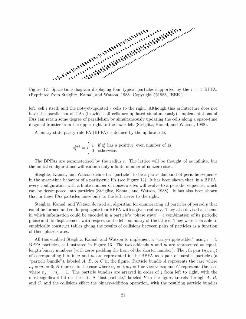
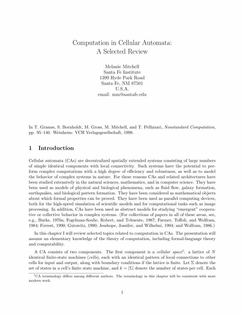
Figure 12: Space-time diagram displaying four typical particles supported by the r = 5 BPFA.(Reprinted from Steiglitz, Kamal, and Watson, 1988. Copyright c©1988, IEEE.)

left, cell i itself, and the not-yet-updated r cells to the right. Although this architecture does nothave the parallelism of CAs (in which all cells are updated simultaneously), implementations ofFAs can retain some degree of parallelism by simultaneously updating the cells along a space-timediagonal frontier from the upper right to the lower left (Steiglitz, Kamal, and Watson, 1988).

A binary-state parity-rule FA (BPFA) is defined by the update rule,

st+1i =

{

1 if ηti has a positive, even number of 1s

0 otherwise.

The BPFAs are parameterized by the radius r. The lattice will be thought of as infinite, butthe initial configurations will contain only a finite number of nonzero sites.

Steiglitz, Kamal, and Watson defined a “particle” to be a particular kind of periodic sequencein the space-time behavior of a parity-rule FA (see Figure 12). It has been shown that, in a BPFA,every configuration with a finite number of nonzero sites will evolve to a periodic sequence, whichcan be decomposed into particles (Steiglitz, Kamal, and Watson, 1988). It has also been shownthat in these FAs particles move only to the left, never to the right.

Steiglitz, Kamal, and Watson devised an algorithm for enumerating all particles of period p thatcould be formed and could propagate in a BPFA with a given radius r. They also devised a schemein which information could be encoded in a particle’s “phase state”—a combination of its periodicphase and its displacement with respect to the left boundary of the lattice. They were then able toempirically construct tables giving the results of collisions between pairs of particles as a functionof their phase states.

All this enabled Steiglitz, Kamal, and Watson to implement a “carry-ripple adder” using r = 5BPFA particles, as illustrated in Figure 13. The two addends n and m are represented as equal-length binary numbers (with zeros padding the front of the shorter number). The jth pair (nj , mj)of corresponding bits in n and m are represented in the BPFA as a pair of parallel particles (a“particle bundle”), labeled A, B, or C in the figure. Particle bundle A represents the case wherenj = mj = 0; B represents the case where nj = 0, mj = 1 or vice versa; and C represents the casewhere nj = mj = 1. The particle bundles are arrayed in order of j from left to right, with themost significant bit on the left. A “fast particle,” labeled F in the figure, travels through A, B,and C, and the collisions effect the binary-addition operation, with the resulting particle bundles

21

F

B A C C A B

Figure 13: Schematic diagram of the operation of the carry-ripple adder of Steigliz, Kamal, andWatson. The “particle-bundles” (pairs of particles) encode the bits of the two addends, and arelabeled A (0,0), B (0,1 or 1,0), and C (1,1). The fast particle, labeled F , effects the addition ofeach pair of addends. Afer collision with F , the particle bundles encode the result for each addedpair, and F propagates the carry bit. (Adapted from Steiglitz, Kamal, and Watson, 1988.)

encoding the result for each added pair, and the F particle encoding the current carry bit. (It isrequired here that the speeds of the particles do not change after collisions, a requirement that isnot hard to implement in BPFAs.) The final F and the final particle bundles transmit the resultsof the addition to the leftmost cell, where they are read off by some external interpreter.

The trick to implement this carry-ripple adder was to find a set of particles that have the desiredbehavior. Steiglitz, Kamal, and Watson sketched a graph-search algorithm (not described here)that searches collision tables for particles implementing any desired logical operation via collisionsbetween a fast particle and slow-particle bundles, as in the carry-ripple addition scheme describedabove.

Steiglitz, Kamal, and Watson’s construction was meant to be an example of how simple arith-metic can be implemented in cellular-automaton-like devices. Other simple logical operations be-sides addition could presumably be implemented in a similar way. Their work differs from mostof the constructions I have described in previous sections in that it is meant to be a practicalmethod for parallel computation rather than a proof of principle or a theoretical result. All thealgorithms they described (e.g., enumerating particles and searching collision tables) were actuallyimplemented and were analyzed in terms of complexity to show that this is a feasible approach. Thenext step is to devise automated methods to efficiently combine these simple arithmetic operationsinto more complicated desired computations, and to demonstrate that these achieve the requisiteparallelism and accompanying speed-up. This is likely to be difficult—as Squier and Steiglitz com-ment in a later paper, “the behavior of the particles is very difficult to control and their propertiesonly vaguely understood.” (Squier and Steiglitz, 1994).

In their later study, Richard Squier and Kenneth Steiglitz (1994) described a possibly moregeneral and more easily programmable approach to computation in CAs using colliding particles.Their “particle machine” approach is closely related to lattice gases, an application of cellularautomata to the simulation of fluid dynamics, in which “particles” are primitive cell states ratherthan more complex space-time structures and local rules are given directly in terms of particlemovements and particle collisions and reactions. (For overviews of research on lattice gases, see,

22

left addend right addend

processor particle

(a)

left multiplicand right multiplicand

processor particles

(b)

Figure 14: Schematic illustration of Squier and Steiglitz’s (a) binary addition and (b) binarymultiplication schemes using particle collisions. (Adapted from Squier and Steiglitz, 1994.)

e.g., Doolen, 1990; Toffoli and Margolus, 1987; and Lawniczak and Kapral, 1996).

Squier and Steiglitz’s particle machines are one-dimensional bounded CAs. A certain number nof particle-types is defined ahead of time by the designer—the idea is to define enough types so asto be able to use this same CA for many different computations. The state of each cell encodes anoccupancy vector which says which particle types are currently occupying the cell (the number ofstates per cell is 2n, the number of possible occupancy configurations). The transition table gives,for every configuration of particles in a neighborhood, what the next state is for the center cell ofthat neighborhood.

To perform a computation, particles are “injected” by an outside agent at different speeds atthe ends of the lattice, propagating along the lattice, colliding with other particles, and takingpart in reactions. It is decided ahead of time what constitutes an answer, and the computation isconsidered to be complete when the answer appears somewhere in the lattice.

Squier and Steiglitz gave several examples to illustrate how particle machines might be pro-grammed. All the examples can be implemented in a single particle machine with r = 1 andn ≈ 14. The first example is a binary-addition scheme, illustrated in Figure 14a, which is similarto the carry-ripple adder scheme described above. Here, the bits of the two addends, n and m, arerepresented by four different types of “data” particles: left- and right-moving 0s and 1s. The bitsof n are injected in the left end of the lattice, least-significant bit first, and likewise for the bits ofm in the right end of the lattice. In the center of the lattice is a stationary “processor” particlepk, which can take on one of two types, p0 or p1, representing a carry bit of 0 or 1, respectively. Itstarts out in state p0. When pk’s neighborhood contains a right-moving data particle on its left anda left-moving data particle on its right, the two data particles are annihilated, a new, left-moving“answer” particle is created that encodes the result of addition mod 2 (with the current carry bit),

23

and pk is set to either p0 or p1, depending on the new carry bit. The left-moving answer particlecan pass unchanged through any additional right-moving data particles. The answer is read off theleft end of the lattice as the answer particles arrive.

A second example is binary multiplication (Figure 14b). Here, as before, data particles encodingthe bits of the two multiplicands n and m travel left and right towards the center of the lattice. Inthe center is a row of processor particles. At each three-way interaction between two data particlesand a processor particle, the processor particle is set to encode the sum of the product of thetwo bits and its previous state (initially set to 0). Any carry bits are encoded by the right-movingparticles. After all the data particles have passed through each other, the processor particles containthe product nm, with the least-significant bit on the left. (Note that this scheme requires knowingahead of time how many processor particles to use for a given n and m.)

Squier and Steiglitz give similar sketches for particle-collision schemes to perform arbitrarilynested combinations of arithmetic operators as well as schemes to perform digital filtering. Theseexamples are meant to illustrate the general framework, which Squier and Steiglitz claim can providea programmable CA substrate for general-purpose parallel computation. (They contrast theirapproach with systolic arrays, e.g., Kung, 1982. Systolic arrays are special-purpose CA-like devicesin which each processor—and sometimes the connection topology—is typically more complicatedthan that in the CAs which we have been discussing). Like the BPFA approach described above,at this point the research into this framework is just beginning; it is as yet unclear how hard it willbe to construct hardware and to write “programs” for this framework for performing more complexcomputations with a useful degree of parallelism. Some discussion of a hardware implementationof this approach is given in Squier, Steiglitz, and Jakubowski (1995).

8 Evolving Cellular Automata with Genetic Algorithms

(This section is adapted from Mitchell, Crutchfield, and Das, 1996.)

In previous sections, I have described several projects in which cellular automata are cleverly(and sometimes with considerable difficulty) hand-designed to perform computations. The work ofmyself and my colleagues James Crutchfield, Rajarshi Das, James Hanson, and Peter Hraber takesa different approach, that of automatically designing CAs with genetic algorithms (GAs).

Genetic algorithms are search methods inspired by biological evolution. In a typical GA, candi-date solutions to a given problem are encoded as bit strings. A population of such strings (“chro-mosomes”) is chosen at random and evolves over several generations under selection, crossover, andmutation. At each generation, the fitness of each chromosome is calculated according to some ex-ternally imposed fitness function, and the highest-fitness chromosomes are selected preferentially toform a new population via reproduction. Pairs of such chromosomes produce offspring via crossover,where each offspring receives components of its chromosome from each parent. The offspring arethen subject to a small probability of mutation at each bit position. After several generations, thepopulation often contains high-fitness chromosomes—high-quality solutions to the given problem.(For overviews of GAs, see Goldberg, 1989 and Mitchell, 1996.)

Some early work on evolving CAs with GAs was done by Packard and colleagues (Packard,1988; Richards, Meyer, and Packard, 1990). Koza (1992) also applied genetic programming toevolve CAs for simple random-number generation. Our work builds on that of Packard (1988),described in Section 4. We have used a form of the GA to evolve CAs to perform two compu-

24

0

Time

148148Site0 148Site0

Figure 15: Space-time diagrams for φmaj, the r = 3 majority rule. In the left diagram, ρ0 < 12 ; in

the right diagram, ρ0 > 12 .

tational tasks. The first is a density-classification task (Mitchell, Hraber, and Crutchfield, 1993;Mitchell, Crutchfield, and Hraber, 1994b; Crutchfield and Mitchell, 1995; and Das, Mitchell, andCrutchfield, 1994.) (Subsequent work on evolving CAs and related architectures to perform densityclassification was done by Sipper, 1996, and by Andre, Bennett, and Koza, 1996.) The second is asynchronization task (Das, Crutchfield, Mitchell, and Hanson, 1995). All the work described hereuses one-dimensional, k = 2, r = 3 CAs with periodic boundary conditions.

For the density classification task, the goal was to find a CA that decides whether or not theinitial configuration (IC) contains a majority of 1s (i.e., has high density). If it does, the wholelattice should eventually go to the fixed-point configuration of all 1s (i.e., all cells in state 1 for allsubsequent iterations); otherwise it should eventually go to the fixed-point configuration of all 0s.More formally, we call this task the “ρc = 1

2” task. Here ρ denotes the density of 1s in a binary-stateCA configuration and ρc denotes a “critical” or threshold density for classification. Let ρ0 denotethe density of 1s in the IC. If ρ0 > ρc, then within M time steps the CA should go to the fixed-pointconfiguration of all 1s (i.e., all cells in state 1 for all subsequent iterations); otherwise, within Mtime steps it should go to the fixed-point configuration of all 0s. M is a parameter of the task thatdepends on the lattice size N .

Designing an algorithm to perform the ρc = 12 task is trivial for a system with a central controller

or central storage of some kind, such as a standard computer with a counter register or a neuralnetwork in which all input units are connected to a central hidden unit. However, the task isnontrivial for a small-radius (r ≪ N) CA, since a small-radius CA relies only on local interactions.It has been proved that no finite-radius, two-state CA with periodic boundary conditions canperform this task perfectly across all lattice sizes (Land and Belew, 1995; Das, 1997), but evento perform this task well for a fixed lattice size requires more powerful computation than canbe performed by a single cell or any linear combination of cells. Since the 1s can be distributedthroughout the CA lattice, the CA must transfer information over large distances (≈ N). To dothis requires the global coordination of cells that are separated by large distances and that cannotcommunicate directly. How can this be done while still exploiting the parallelism of CAs? Ourinterest was to see if the GA could devise one or more methods.

25

The need for such coordination is illustrated in Figure 15, in which we display the space-timebehavior of a naive hand-designed candidate solution for this task—the “majority” rule φmaj, inwhich the output bit for each 7-bit (r = 3) neighborhood is decided by a majority vote among theseven cells in the neighborhood. Figure 15 gives two space-time diagrams displaying the behaviorof this rule on two initial conditions, one with ρ0 < 1/2 and the other with ρ0 > 1/2. As can beseen, local neighborhoods with majority 1s map to regions of all 1s and similarly for 0s, but whenan all-1s region and an all-0s region border each other, there is no way to decide between them,and both persist. Thus, the majority rule (which implements a threshold on a linear combinationof states) does not perform the ρc = 1

2 task.

Instead, more sophisticated coordination and information transfer must be achieved. This coor-dination must, of course, happen in the absence of any central processor or central memory directingthe coordination.

We used a genetic algorithm to search for k = 2, r = 3 CA rules to perform the ρc = 12 task. Each

chromosome in the population represented a candidate CA rule—it consisted of the output bits ofthe rule table, listed in lexicographic order of neighborhood (cf. φ in Figure 1). The chromosomesrepresenting rules were thus of length 22r+1 = 128. The size of the rule space in which the GAworked was thus 2128—far too large for any kind of exhaustive evaluation.

Our version of the GA worked as follows. First, a population of 100 chromosomes was chosen atrandom from a distribution that was flat over the density of 1s in the output bits. (This “uniform”distribution differs from the more commonly used “unbiased” distribution in which each bit inthe chromosome is independently randomly chosen. We found that using a uniform distributionconsiderably improved the GA’s performance on this task—see Mitchell, Crutchfield, and Hraber,1994b, for details). The fitness of a rule in the population was computed by (1) randomly choosing100 ICs that are uniformly distributed over ρ ∈ [0.0, 1.0], with exactly half with ρ < ρc and halfwith ρ > ρc, (2) iterating the rule on each IC until it arrives at a fixed point or for a maximum ofM ≈ 2N time steps, and (3) determining whether the final behavior is correct—that is, 149 0s forρ0 < ρc and 149 1s for ρ0 > ρc. The rule’s fitness, F100, was the fraction of the 100 ICs on whichthe rule produced the correct final behavior. No partial credit was given for partially correct finalconfigurations. (Like the initial population of rules, each sample of ICs on which to test the ruleswas chosen from a uniform distribution rather than an unbiased distribution over ρ because theformer considerably improved the GA’s performance on this problem.)

In each generation, a new set of 100 ICs was generated; F100 was computed for each rule in thepopulation; CAs in the population were ranked in order of fitness; the 20 highest fitness (“elite”)rules were copied to the next generation without modification; and the remaining 80 rules for thenext generation were formed by single-point crossovers between randomly chosen pairs of elite rules.The parent rules were chosen from the elite with replacement—that is, an elite rule was permittedto be chosen any number of times. The offspring from each crossover were each mutated at exactlytwo randomly chosen positions. This process was repeated for 100 generations for a single runof the GA. (Since a different sample of ICs was chosen at each generation, the fitness functionwas stochastic.) For a discussion of this algorithm and details of its implementation, see Mitchell,Crutchfield, and Hraber (1994b).

In our experiments, we set N = 149, a reasonably large but still computationally tractable oddnumber (odd, so that the task will be well-defined on all ICs).

Six hundred runs were performed, each starting with a different random-number seed. Weexamined the fittest evolved rules to understand their computational “strategies” for performing

26

CA (r = 3) Rule table (hex) P149,104 P599,104 P999,104

φmaj 000101170117177f 0.000 0.000 0.000

0117177f177f7fffφexp 0505408305c90101 0.652 0.515 0.503

200b0efb94c7cff7φpar 0504058705000f77 0.769 0.725 0.714

037755837bffb77f

Table 2: Rule tables and measured values of PN ,104(φ) at various N for three different r = 3 rules.To recover the 128-bit string giving the output bits of the rule table, expand each hexadecimaldigit (the first row followed by the second row) to binary. The output bits are then given inlexicographic order starting from the all-0s neighborhood at the leftmost bit in the 128-bit binarystring. φmaj (hand-designed) computes the majority of 1s in the neighborhood. φexp (evolved bythe GA) expands blocks of 1s. φpar (evolved by the GA) uses a “particle-based” strategy.

0

Time

148

148Site0 148Site0

Figure 16: Space-time diagrams for a “block-expanding” rule, φexp. In the left diagram, ρ0 < 1/2;in the right diagram, ρ0 > 1/2. Both ICs are correctly classified.

the density classification task. On most runs the GA evolved a rather unsophisticated class ofstrategies. One example, a CA here called φexp (for “expand”), is illustrated in Figure 16. Thisrule had F100 ≈ 0.9 in the generation in which it was discovered. Its computational strategy is thefollowing: Quickly reach the fixed point of all 0s unless there is a sufficiently large block of adjacent(or almost adjacent) 1s in the IC. If so, expand that block. (For this rule, “sufficiently large” is 7 ormore cells.) This strategy does a fairly good job of classifying low and high density ICs under F100:it relies on the appearance or absence of blocks of 1s to be good predictors of ρ0, since high-densityICs are statistically more likely to have blocks of adjacent 1s than low-density ICs.

Similar strategies were evolved in most runs. On approximately half the runs, “expand 1s”strategies were evolved, and on most of the other runs, the opposite “expand 0s” strategies wereevolved. These block-expanding strategies, although they obtained F100 ≈ .9 with N = 149, donot count as sophisticated examples of computation in CAs: all the computation is done locally inidentifying and then expanding a “sufficiently large” block. There is no notion of global coordinationor information flow between distant cells—two things we claimed were necessary to perform wellon the task. Indeed, such strategies perform poorly under performance measures using different

27

0

Time

148

148Site0 148Site0

Figure 17: Space-time diagrams for φpar, a “particle-based” rule. In the left diagram, ρ0 < 1/2; inthe right diagram, ρ0 > 1/2. Both ICs are correctly classified. The gray-looking region consists ofa checkerboard pattern of alternating 0s and 1s.

distributions of ICs, and when N is increased. This can be seen in Table 2, which gives the ruletables and performances across different lattice sizes for different rules. The performance PN ,104 isdefined as the fraction of correct classifications over 104 ICs chosen at random from the unbiaseddistribution (each bit in the IC is independently randomly chosen). This is a more difficult testof quality than F100: since they are chosen from an unbiased distribution, these ICs all have ρ0

close to 1/2 and are thus the hardest cases to classify. Therefore, PN ,104 gives a lower bound onother performance measures. As can be seen, PN ,104(φmaj) was measured to be zero for each N .PN ,104(φexp) is approximately 0.65 for N = 149 and drops to approximately 0.5 for the larger valuesof N .

Mitchell, Crutchfield, and Hraber (1994b) analyzed the detailed mechanisms by which the GAevolved such block-expanding strategies. This analysis uncovered some quite interesting aspectsof the GA, including a number of impediments that, on most runs, kept the GA from discoveringbetter-performing CAs. These included the GA’s breaking the ρc = 1

2 task’s symmetries for short-term gains in fitness, as well as “overfitting” to the fixed lattice size N = 149 and the unchallengingnature of the IC samples.

Despite these various impediments and the unsophisticated CAs evolved on most runs, on ap-proximately 3% percent of the runs the GA discovered CAs with more sophisticated strategies thatyielded significantly better performance across different IC distributions and lattice sizes than wasachieved by block-expanding strategies. The typical space-time behaviors of one such rule, herecalled φpar (for “particle”), are illustrated in Figure 17.

The improved performance of φpar can be seen in table 2. φpar not only has significantly higherperformance than φexp for N = 149, but its performance degrades relatively slowly as N is increased,whereas φexp’s performance drops quickly. As we describe in Das, Mitchell, and Crutchfield (1994),φpar’s behavior is similar to that of a CA designed by Gacs, Kurdyumov, and Levin (1978).

In Figure 17 it can be seen that, under φpar, there is a transient phase during which spatialand temporal transfer of information about the density in local regions takes place. Roughly, overshort times, φpar’s behavior is locally similar to that of φmaj in that local high-density regions

28

Regular DomainsΛ0 = 0∗ Λ1 = 1∗ Λ2 = (01)∗

Particles (Velocities)α ∼ Λ0Λ1 (0) β ∼ Λ101Λ0 (0)γ ∼ Λ0Λ2 (-1) δ ∼ Λ2Λ0 (-3)η ∼ Λ1Λ2 (3) µ ∼ Λ2Λ1 (1)

Interactionsdecay α → γ + µ

react β + γ → η, µ + β → δ, η + δ → β

annihilate η + µ → Ø, γ + δ → Ø

Table 3: Catalog of regular domains, particles (domain boundaries), particle velocities (in paren-theses), and particle interactions seen in φpar’s space-time behavior. The notation p ∼ ΛxΛy meansthat p is the particle forming the boundary between regular domains Λx and Λy. Ø denotes anannihilation (no particles are formed by the interaction).

are mapped to all 1s, local low-density regions are mapped to all 0s, with a vertical boundary inbetween them. This is what happens when a region of 1s on the left meets a region of 0s on the right.However, there is a crucial difference from φmaj: when a region of 0s on the left meets a region of1s on the right, rather than a vertical boundary being formed, a checkerboard region (alternating1s and 0s, appearing “gray” in the figure) is propagated. When the propagating checkerboardregion collides with the black-white boundary, the inner region (e.g., the large white region in theright-hand diagram of Figure 17) is cut off and the outer region is allowed to propagate. In thisway, the CA uses local interactions and geometry to determine the relative sizes of adjacent low-and high-density regions that are larger than the neighborhood size. For example, in the right-handspace-time diagram, the large inner white region is smaller than the large outer black region. Thusthe propagating checkerboard pattern reaches the black-white boundary on the white side beforeit reaches it on the black side; the former is cut off, and the latter is allowed to propagate.

The black-white boundary and the checkerboard region can be thought of as “signals” indicating“ambiguous” regions. The creation and interactions of these signals can be interpreted as the locusof the computation being performed by the CA—they form its emergent “algorithm.”

The above explanation of how φpar performs the ρc = 12 task is informal and incomplete. Our

approach to a more rigorous understanding is to examine the space-time behavior exhibited by theCA and to “reconstruct” from that behavior what the emergent algorithm is, using Crutchfieldand Hanson’s computational mechanics framework (Section 4). Recall that regular domains are(roughly) regions of space-time consisting of words in the same regular language—in other words,they are regions that are computationally homogeneous and simple to describe. E.g., in figure 17,there are three regular domains, corresponding to the regular languages 0∗, 1∗, and (01)∗. Particlesare defined to be the localized boundaries between those domains. In computational mechanics,particles are identified as information carriers, and collisions between particles are identified as theloci of information processing. Particles and particle interactions form a high-level language fordescribing computation in spatially extended systems such as CAs. Figure 18 hints at this higherlevel of description: to produce it we filtered the regular domains from the space-time behaviordisplayed in the right-hand diagram of figure 17 to leave only the particles and their interactions,in terms of which the emergent algorithm of the CA can be understood. Table 3 gives a catalogof the relevant particles and interactions for φpar. In Crutchfield and Mitchell (1995) and in Das(1997) we describe other particle-based rules that were evolved by the GA for this task. In Das,Mitchell, and Crutchfield (1994) we describe the evolutionary stages by which φpar was evolved by

29

148Site0

γ µ

η

βδ

α

β

148Site0

0

148

Time

Figure 18: (a) The right-hand spacetime diagram of figure 17. (b) The same diagram with theregular domains filtered out, leaving only the particles (some of which are labeled by here by theGreek letter code of table 3). Note that particle α (unlike other the other particles) lasts for onlyone time step, after which it decays to particles γ and µ.

the GA.

In Das, Crutchfield, Mitchell, and Hanson (1995), we gave a similar analysis for a global syn-chronization task. The goal for the GA was to find a CA that, from any IC, produces a globallysynchronous oscillation between the all-1s and all-0s configurations. This task differs considerablyfrom the FSSP. First, the FSSP uses cells with many states, allowing for boundary cells, a “general”cell, and a diverse array of signals. In contrast, we are using two-state CAs with periodic boundaryconditions, so there can be no special cells or propagating signals based on different local states.Instead, like in the density-classification task, “signals” have to emerge as particles—boundariesbetween regular domains formed by cells in state 0 or 1. Second, the desired final behavior is notstatic as in the FSSP, but is dynamic—an oscillation between all 1s and all 0s. Third, in our tasksynchronization must take place starting from any IC, rather than all cells starting in the quiescentstate as in the FSSP. We believe that all of these features make this task more interesting and makeit require solutions that will be more similar to the emergence of spontaneous synchronization thatoccurs in decentralized systems throughout nature.

Figure 19 illustrates the behavior of one CA, here called φsync, evolved by the GA to performthis task. The behavior is illustrated both as a space-time diagram and as a filtered version of thatdiagram which reveals the embedded particles. The basic strategy of φsync is similar in some waysto that of φpar for the density-classification task. Local regions of synchrony can be formed easily byrequiring that the all-0s neighborhood maps to 1 and the all-1s neighborhood maps to 0. However,as can be seen in Figure 19a, those local regions can be out of phase with one another. φsync usesparticles—boundaries between the synchronized regions and the jagged regions—to allow one localphase to take over the entire lattice by cutting off other local phases.

Again, tools of computational mechanics allowed us to understand φsync’s strategy in the higher-level language of particles and particle interactions (Figure 19b) as opposed to the low-level languageof CA rule tables and detailed spatial configurations. This is described in detail in Das, Crutchfield,Mitchell, and Hanson (1995).

30

Site0 74Site0 74

0

74

Time

(a) (b)

Figure 19: (a) Space-time diagram illustrating the behavior of a CA evolved by the GA to performthe synchronization task. The initial condition was generated at random. (b) The same space-timediagram after filtering out regular domains.

Our notion of computation via particles and particle-interactions differs considerably from thenotions used in the work presented in previous sections. Propagating particle-like signals were usedin the solution to the FSSP and in Smith’s formal-language recognizers, but those were designed byhand to be the explicit behavior of the CA, and their interactions were effected by a relatively largenumber of states. Steiglitz, Kamal, and Watson’s carry-ripple adder and the universal computerconstructed in the Game of Life both used binary-state signals consisting of propagating periodicpatterns, but again, the particles were explicit against a quiescent background, and their interactionproperties were carefully hand coded. Squier and Steiglitz’s particles were the primitive states ofthe cells and their interaction properties were explicit in the CA rule.

In contrast to all these systems, particles in our system are “embedded” as walls between regulardomains, and are often apparent only after those domains have been discovered and filtered out.Their structures and interaction properties are “emergent” properties of the patterns formed by theCAs, and although each cell has only two possible states, the structures of embedded particles canbe more complex than atomic or simple periodic structures. Finally, in contrast to Crutchfield andHanson’s work on computational mechanics of CAs, in our work particles and their interactionsattain semantics, in that they contribute to an overall strategy for accomplishing a desired task.For example, in Figure 18(b), the γ particle can be interpreted as signaling a particular kind ofambiguity—a white region bordering a black region each of size greater than 2r +1. Its interactionwith the β particle and the subsequent creation of the η particle can be interpreted as signaling thatthe white region was smaller than the black region. This kind of interpretation contrasts with thenon-semantic particles of Figure 8b. In the case of φpar, these kind of semantics can be attached toparticles and their interactions only in virtue of the evolutionary selection pressures to which theCA’s lineage has been subject.

More generally, our philosophy is to view CAs as systems that naturally form patterns (suchas regular domains), and to view the GA as taking advantage—via selection and variation—ofthese pattern-forming propensities so as to shape them to perform desired computations. Wethen attempt to understand the behavior of the resulting CAs by applying tools (such as the

31

computational mechanics framework) formulated for analyzing pattern-forming systems, which giveus a high-level description of the computationally relevant parts of the system’s behavior. In doingso, we begin to answer Wolfram’s last problem from “Twenty problems in the theory of cellularautomata” (Wolfram, 1985): “What higher-level descriptions of information processing in cellularautomata can be given?”, and we believe that this framework will be a basis for the “radically newapproach” that Wolfram thinks will be needed.

This approach is motivated in part by our interest in developing scientific tools for understandinghow systems in nature perform computations. However, we also believe that the best approachto engineering highly complex, massively parallel, and decentralized computing systems will be totake advantage of the natural dynamics of such systems in the same way that natural evolutiontakes advantage of the intrinsic dynamics of the systems on which it operates.

While our work on evolving CAs with GAs is a highly simplified example of this overall approach,the GA’s discoveries of rules such as φpar and of rules that produce global synchronization issignificant, since these are the first examples of a GA’s producing sophisticated computation indecentralized, distributed systems. These discoveries are encouraging for the prospect of usingGAs to automatically evolve computation for more complex tasks (e.g., image processing or imagecompression) and in more complex systems; these are the subjects of current work by our group.Moreover, evolving CAs with GAs also gives us a tractable framework in which to study themechanisms by which an evolutionary process might create complex coordinated behavior in naturaldecentralized distributed systems. For example, we have already learned how the GA’s breakingof symmetries can lead to suboptimal computational strategies (Mitchell, Crutchfield, and Hraber,1993); eventually we may be able to use such models to test ways in which such symmetry breakingmight occur in natural evolution. In general, models such as ours can provide insights on howevolutionary processes can discover structural properties of individuals that give rise to improvedadaptation. In our case, such structural properties—regular domains and particles—were identifiedvia the computational mechanics framework, and allowed us to analyze the evolutionary emergenceof sophisticated computation.

9 Conclusion

This review has only begun to describe the large literature on computation in cellular automata,and the even larger literature on decentralized parallel computation in general. Some of the recentwork on these topics is brought together in the Parcella proceedings (Handler, Legendi, and Wolf,1995; Legendi et al., 1986; Wolf, Legendi, and Schendel, 1988; Wolf, Legendi, and Schendel, 1990;Jesshope, Jossifov, and Wilhelmi, 1994).

Among the important topics that were left out are discussions of hardware implementations ofCAs (e.g., Toffoli and Margolus, 1987); reliable computation in CAs (e.g., Gacs, 1986); a largerdiscussion of analysis of CAs in terms of computation theory (e.g., Wolfram, 1984b, Nordahl, 1989,Moore, 1996), computation in more complex CA architectures, including three-dimensional CAs(e.g., Tsalides, Hicks, and York, 1989), CAs with real-valued states (e.g., Garzon and Botelho,1993), and systolic arrays (e.g., Kung, 1982), and the many applications CAs and CA-like archi-tectures have found in parallel computation.

The theory and applications of CAs and similar systems will likely attract increasing interestas the capabilities for massive parallel computation expand, and robust, decentralized, and highlydistributed systems become imperative. CAs and similar systems will also be increasingly important

32

as modeling tools, as scientists probe more deeply into the behavior of natural systems composedof simple components with local communication and emergent collective properties. I hope thatthis review will contribute to the increase of interest in CAs and to the better understanding andwider application of such systems.

10 Acknowledgments

Thanks to Jim Crutchfield, Howard Gutowitz, Jim Hanson, Chris Langton, Cris Moore, and MatsNordahl for many discussions about cellular automata and for comments on an earlier draft of thischapter. This work has been supported by the Santa Fe Institute and by grants from the NationalScience Foundation (IRI-9320200), the Department of Energy (DE-FG03-94ER25231), and theDefense Advanced Projects Research Agency and the Office of Naval Research (N00014-95-1-0975).

References

[1] Andre, D., Bennett, F. H. III, and Koza, J. R. (1996): Evolution of intricate long-distancecommunication signals in cellular automata using genetic programming. In Artificial Life V:Proceedings of the Fifth International Workshop on the Synthesis and Simulation of LivingSystems. Cambridge, MA: MIT Press.

[2] Balzar, R. (1967): An 8-states minimal time solution to the firing squad synchronizationproblem. Information and Control, 10, 22–42.

[3] Banks, E. R. (1971): Information and Transmission in Cellular Automata. Ph.D. Disserta-tion, Massachusetts Institute of Technology.

[4] Berlekamp, E., Conway, J. H., and Guy, R. (1982): Winning Ways for Your MathematicalPlays, volume 2. Academic Press.

[5] Bucher W. and Culik, K. II (1984): On real time and linear time cellular automata. RAIROInformatique Theorique, 18 (4), 307–325.

[6] Burks, A. W. (1966): Editor’s introduction. In von Neumann (1966).

[7] Burks, A. W. (editor) (1970a) . Essays on Cellular Automata. Urbana, IL: University ofIllinois Press.

[8] Burks, A. W. (1970b): Introduction. In Burks (1970a).

[9] Burks, A. W. (1970c): Von Neumann’s self-reproducing automata. In Burks (1970a).

[10] Choffrut, C. and Culik, K. II (1984): On real-time cellular automata and trellis automata.Acta Informatica, 21, 393–407.

[11] Clementi, A., De Biase, G. A., and Massini, A. (1994): Fast parallel arithmetic on cellularautomata. Complex Systems, 8(6), 435.

[12] Codd, E. F. (1968): Cellular Automata. New York: Academic Press.

33

[13] Cole, S. N. (1969): Real-time computation by n-dimensional iterative arrays of finite-statemachines. IEEE Transactions on Computers, 18, 349–365.

[14] Crutchfield, J. P. (1994): The calculi of emergence: Computation, dynamics, and induction.Physica D 75: 11-54.

[15] Crutchfield, J. P., and Hanson, J. E. (1993): Turbulent pattern bases for cellular automata.Physica D 69: 279–301.

[16] Crutchfield, J. P., and Mitchell, M. (1995): The evolution of emergent computation. Proceed-ings of the National Academy of Sciences, USA, 92 (23): 10742.

[17] Crutchfield, J. P., and Young, K. (1989): Inferring statistical complexity. Physical ReviewLetters, 63, 105.

[18] Crutchfield, J. P., and Young, K. (1990): Computation at the onset of chaos. In W. H.Zurek (editor), Complexity, Entropy, and the Physics of Information. Reading, MA: Addison-Wesley.

[19] Culik, K. II (1989): Variations of the firing squad problem and applications. InformationProcessing Letters, 30, 153–157.

[20] Das, R. (1997): The Evolution of Emergent Computation in Cellular Automata. Ph.D. Thesis,Computer Science Department, Colorado State University, Ft. Collins, CO.

[21] Das, R., Crutchfield, J. P., Mitchell, M., and Hanson, J. E. (1995): Evolving globally syn-chronized cellular automata. In L. J. Eshelman, ed., Proceedings of the Sixth InternationalConference on Genetic Algorithms, 336–343. San Francisco, CA: Morgan Kaufmann.

[22] Das, R., Mitchell, M., and Crutchfield, J. P. (1994): A genetic algorithm discovers particle-based computation in cellular automata. In Y. Davidor, H.-P. Schwefel, and R. Manner, eds.,Parallel Problem Solving from Nature—PPSN III, 244-353. Berlin: Springer-Verlag (LectureNotes in Computer Science, volume 866):

[23] Doolen, G. (editor) (1990): Lattice Gas Methods for Partial Differential Equations. Reading,MA: Addison-Wesley.

[24] Eloranta, K. (1994): The dynamics of defect ensembles in one-dimensional cellular automata.Journal of Statistical Physics, 76(5 / 6):1377.

[25] Eloranta, K. and Nummelin, E. (1992): The kink of cellular automaton rule 18 performs arandom walk. Journal of Statistical Physics, 69: 1131-1136.

[26] Farmer, D., Toffoli, T., and Wolfram, S. (editors) (1984): Cellular Automata: Proceedings ofan Interdisciplinary Workshop. Amsterdam: North Holland.

[27] Fischer, P. C. (1965): Generation of primes by a one-dimensional real-time iterative array.Journal of the Association for Computing Machinery, 12 (3), 388–394.

[28] Fogelman-Soulie, F., Robert, Y., and Tchuente, M (1987): Automata Networks in ComputerScience: Theory and Applications. Manchester, UK : Manchester University Press.

[29] Forrest, S. (1990): Emergent computation: Self-organizing, collective, and cooperative phe-nomena in natural and artificial computing networks. Physica D 42: 1–11.

34

[30] Fredkin, E. and Toffoli, T. (1982): Conservative logic. International Journal of TheoreticalPhysics, 21, 219–253.

[31] Gacs, P. (1986): Reliable computation with cellular automata. Journal of Computer andSystems Sciences, 32, 15–78.

[32] Gacs, P., Kurdyumov, G. L., and Levin, L. A. (1978): One-dimensional uniform arrays thatwash out finite islands. Problemy Peredachi Informatsii 14: 92–98 (in Russian).

[33] Garzon, M., and Botelho, F. (1993): Real computation with cellular automata. In Boccara,N. et al. (editors), Cellular Automata and Cooperative Systems, 191–202.

[34] Goldberg, D. E. (1989): Genetic Algorithms in Search, Optimization, and Machine Learning.Reading, MA: Addison-Wesley.

[35] Gould, S. J., and Vrba, E. S. (1982): Exaptation: A missing term in the science of form.Paleobiology 8: 4–15.

[36] Gutowitz, H. A. (1990): Cellular Automata. Cambridge, MA: MIT Press.

[37] Handler, W., Legendi, T., and Wolf, G. (editors) (1985): International Workshop on ParallelProcessing by Cellular Automata and Arrays (Parcella ’84). Berlin : Akademie Verlag

[38] Hanson, J. E. (1993): Computational Mechanics of Cellular Automata. Ph.D. Thesis, PhysicsDepartment, University of California, Berkeley, CA.

[39] Hanson, J. E., and Crutchfield, J. P. (1992): The attractor-basin portrait of a cellular au-tomaton. Journal of Statistical Physics 66, no. 5/6: 1415–1462.

[40] Hofstadter, D. R. (1979): Godel, Escher, Bach: an Eternal, Golden Braid. New York: BasicBooks.

[41] Hopcroft, J. E. and Ullman, J. D. (1979): Introduction to Automata Theory, Languages, andComputation. Reading, MA: Addison-Wesley.

[42] Jesshope, C., Jossifov, V., and Wilhelmi, W. (editors) (1994): International Workshop onParallel Processing by Cellular Automata and Arrays (Parcella ’94). Berlin : AkademieVerlag

[43] Koza, J. R. (1992): Genetic Programming: On the Programming of Computers by Means ofNatural Selection. Cambridge, MA: MIT Press.

[44] Kung, H. T. (1982): Why systolic architectures? Computer, 15, 1 37–46.

[45] Land, M., and Belew, R. K. (1995): No perfect two-state cellular automata for densityclassification exists. Physical Review Letters 74 (25): 5148.

[46] Langton, C. G. (1984): Self-reproduction in cellular automata. Physica D, 10: 135–144.

[47] Langton, C. G. (1990): Computation at the edge of chaos: Phase transitions and emergentcomputation. Physica D, 42, 12-27.

[48] Lawniczak, A. T. and Kapral, R. (editors) (1996): Pattern Formation and Lattice Gas Au-tomata. Oxford: Oxford University Press.

35

[49] Legendi, T. et al. (Editors) (1986): International Workshop on Parallel Processing by CellularAutomata and Arrays (Parcella ’86). Berlin : Akademie Verlag

[50] Li, W., and Packard, N. (1990): The structure of the elementary cellular automata rule space.Complex Systems, 4, 281–297. 7

[51] Lindgren, K. and Nordahl, M. G. (1990): Universal computation in simple one-dimensionalcellular automata. Complex Systems, 4, 299–318.

[52] Margolus, N. (1984): Physics-like models of computation. Physica D, 10, 81–95.

[53] Mazoyer, J. (1987): A six states minimal time solution to the firing squad synchronizationproblem. Theoretical Computer Science, 50, 183–238.

[54] Mazoyer, J. (1988): An overview of the firing squad synchronization problem. In C. Choffurt(editor), Automata Networks: 82–93. Lecture Notes in Computer Science, Vol. 316. Springer-Verlag.

[55] Mazoyer, J. (1996): Computations on one-dimensional cellular automata. Annals of Mathe-matics and Artificial Intelligence, 16 (1–4).

[56] Minsky, M. (1967): Computation: Finite and Infinite Machines. Englewood Cliffs, NJ:Prentice-Hall.

[57] Mitchell, M. (1996): An Introduction to Genetic Algorithms. Cambridge, MA: MIT Press.

[58] Mitchell, M., Crutchfield, J. P., and Das, R. (1996): Evolving cellular automata to performcomputations: A review of recent work. In Proceedings of the First International Conferenceon Evolutionary Computation and Its Applications (EvCA‘96). Moscow, Russia: RussianAcademy of Sciences.

[59] Mitchell, M., Crutchfield, J. P., and Hraber, P. T. (1994a): Dynamics, computation, andthe “edge of chaos”: A re-examination. In G. Cowan, D. Pines, and D. Melzner (editors),Complexity: Metaphors, Models, and Reality. Reading, MA: Addison-Wesley.

[60] Mitchell, M., Crutchfield, J. P., and Hraber, P. T. (1994b): Evolving cellular automata toperform computations: Mechanisms and impediments. Physica D 75: 361–391.

[61] Mitchell, M., Hraber, P. T., and Crutchfield, J. P. (1993): Revisiting the edge of chaos:Evolving cellular automata to perform computations. Complex Systems 7, 89–130.

[62] Moore, C. (1996): Majority-Vote Cellular Automata, Ising Dynamics, and P-Completeness.Working Paper 96-08-060, Santa Fe Insitute, Santa Fe, NM.

[63] Moore, E. F. (1964): The firing squad synchronization problem. In E. F. Moore (editor),Sequential Machines: Selected Papers, 213–214. Reading, MA: Addison-Wesley.

[64] Moore, F. R. and Langdon, G. G. (1968): A generalized firing squad problem. Informationand Control, 12, 212–220.

[65] Nordahl, M. G. (1989): Formal languages and finite cellular automata. Complex Systems, 3,63–78.

36

[66] Packard, N. H. (1988): Adaptation toward the edge of chaos. In J. A. S. Kelso, A. J. Mandell,M. F. Shlesinger, eds., Dynamic Patterns in Complex Systems, 293–301. Singapore: WorldScientific.

[67] Pecht, J. (1983): On the real-time recognition of formal languages in cellular automata. ActaCybernetica 6 (1): 33-53.

[68] Pesavento, U. (1996). An implementation of von Neumann’s self-reproducing machine. Arti-ficial Life 2 (4), 337-354.

[69] Poundstone, W. (1985): The Recursive Universe: Cosmic Complexity and the Limits ofScientific Knowledge. New York: Morrow.

[70] Richards, F. C., Meyer, T. P., and Packard, N. H. (1990): Extracting cellular automatonrules directly from experimental data. Physica D 45: 189–202.

[71] Seiferas, J. I. (1977): Linear-time computation by nondeterministic multi-dimensional itera-tive arrays. SIAM Journal of Computing, 6, 487–504.

[72] Sheth, B., Nag, P., and Hellwarth, R. W. (1991): Binary addition on cellular automata.Complex Systems, 5, 479.

[73] Shinahr, I. (1974): Two and three-dimensional firing squad synchronization problems. Infor-mation and Control, 24, 163–180.

[74] Sipper, M. (1996): Co-evolving non-uniform cellular automata to perform computations.Physica D, 92: 193–208.

[75] Smith, A. R. III (1971): Simple computation-universal cellular spaces. Journal of the Asso-ciation for Computing Machinery, 18, 339–353.

[76] Smith, A. R. III (1972): Real-time language recognition by one-dimensional cellular automata.Journal of Computer and System Sciences, 6, 233–253.

[77] Sommerhalder, R. and van Westrhenen, S. C. (1983): Parallel language recognition in con-stant time by cellular automata. Acta Informatica, 19, 397.

[78] Squier, R. K. and Steiglitz, K. (1994): Programmable parallel arithmetic in cellular automatausing a particle model. Complex Systems, 8, 311–323.

[79] Squier, R. K., Steiglitz, K., and Jakubowski, M. H. (1995): General Parallel ComputationWithout CPUs: VLSI Realization of a Particle Machine. Technical Report TR-484-95, Com-puter Science Department, Princeton University, Princeton, NJ.

[80] Steiglitz, K., Kamal, I., and Watson, A. (1988): Embedding computation in one-dimensionalautomata by phase-coding solutions. IEEE Transactions on Computers, 37, 138–145.

[81] Terrier, V. (1994): Language recognizable in real time by cellular automata. Complex Sys-tems, 8, 325–336.

[82] Toffoli, T., and Margolus, N. (1987): Cellular Automata Machines: A New Environment forModeling. Cambridge, MA: MIT Press.

37

[83] Tsalides, Ph., Hicks, P. J., and York, T. A. (1989): Three-dimensional cellular automata andVLSI applications. IEE Proceedings, 136, Pt. E, No. 6, 490–495

[84] von Neumann, J. (1966): Theory of Self-Reproducing Automata (edited and completed by A.W. Burks). Urbana, IL: University of Illinois Press.

[85] Waksman, A. (1966): An optimum solution to the firing squad synchronization problem.Information and Control, 9, 66–78.

[86] Wolf, G., Legendi, T., and Schendel, U. (Editors) (1988): International Workshop on ParallelProcessing by Cellular Automata and Arrays (Parcella ’88). Berlin : Springer-Verlag.

[87] Wolf, G., Legendi, T., and Schendel, U. (Editors) (1990): International Workshop on ParallelProcessing by Cellular Automata and Arrays (Parcella ’90). Berlin : Akademie-Verlag.

[88] Wolfram, S. (1983): Statistical mechanics of cellular automata. Review of Modern Physics,55, 601–644,

[89] Wolfram, S. (1984a): Universality and complexity in cellular automata. Physica D, 10, 1–35.

[90] Wolfram, S. (1984b): Computation theory of cellular automata. Communications in Mathe-matical Physics, 96, 15–57.

[91] Wolfram, S. (1985): Twenty problems in the theory of cellular automata. Physica Scripta,T9, 170–183.

[92] Wolfram, S. (editor) (1986): Theory and Applications of Cellular Automata. Singapore:World Scientific.

[93] Yunes, J. B. (1994): Seven-state solutions to the firing squad synchronization problem. The-oretical Computer Science, 127, 313–332.

38