computation and numerics in neurostimulation
TRANSCRIPT

Computation and Numerics in Neurostimulation
Edward T. Dougherty
Dissertation submitted to the Faculty of theVirginia Polytechnic Institute and State University
in partial fulfillment of the requirements for the degree of
Doctor of Philosophyin
Genetics, Bioinformatics, and Computational Biology
James C. Turner, ChairDavid R. BevanKathleen O’HaraRyan S. Senger
April 17, 2015Blacksburg, Virginia
Keywords: Simulation, Neurostimulation, Numerical Methods
Copyright 2015, Edward T. Dougherty

Computation and Numerics in Neurostimulation
Edward T. Dougherty
Abstract
Neurostimulation continues to demonstrate tremendous success as an intervention for neu-rodegenerative diseases, including Parkinson’s disease, in addition to a range of other neuro-logical and psychiatric disorders. In an effort to enhance the medical efficacy and comprehen-sion of this form of brain therapy, modeling and computational simulation are regarded asvaluable tools that enable in silico experiments for a range of neurostimulation research en-deavours. To fully realize the capacities of neurostimulation simulations, several areas withincomputation and numerics need to be considered and addressed. Specifically, simulationsof neurostimulation that incorporate (i) computational efficiency, (ii) application versatility,and (iii) characterizations of cellular-level electrophysiology would be highly propitious insupporting advancements in this medical treatment.
The focus of this dissertation is on these specific areas. First, preconditioners and iterativemethods for solving the linear system of equations resulting from finite element discretiza-tions of partial differential equation based transcranial electrical stimulation models arecompared. Second, a software framework designed to efficiently support the range of clini-cal, biomedical, and numerical simulations utilized within the neurostimulation communityis presented. Third, a multiscale model that couples transcranial direct current stimulationadministrations to neuronal transmembrane voltage depolarization is presented. Fourth, nu-merical solvers for solving ordinary differential equation based ligand-gated neurotransmitterreceptor models are analyzed.
A fundamental objective of this research has been to accurately emulate the unique medicalcharacteristics of neurostimulation treatments, with minimal simplification, thereby provid-ing optimal utility to the scientific research and medical communities. To accomplish this, nu-merical simulations incorporate high-resolution, MRI-derived three-dimensional head mod-els, real-world electrode configurations and stimulation parameters, physiologically-basedinhomogeneous and anisotropic tissue conductivities, and mathematical models accepted bythe brain modeling community. It is my hope that this work facilitates advancements inneurostimulation simulation capabilities, and ultimately helps improve the understandingand treatment of brain disease.

Dedication
To my mom- for your support, wisdom, and love throughout the years.
iii

Acknowledgements
I would like to acknowledge and express my gratitude to several individuals for their contri-butions to this research project and my years as a doctoral student.
My advisor, James Turner, for working closely with me over the past four years, and givingme the independence to pursue my research interests. I am especially grateful for his adviceand wisdom during challenging academic and personal times.
My doctoral committee - David Bevan, Kathleen O’Hara, and Ryan Senger - for their valu-able input, comments and encouragement.
Our collaborator Frank Vogel and the entire inuTech team for their valuable assistance withthe Diffpack software application.
My family, for their confidence and love.
Angie and Sadie, for your support, encouragement, patience, and love.
iv

Contents
1 Introduction 1
1.1 Overview . . . . . . . . . . . . . . . . . . . . . . . . . . . . . . . . . . . . . . 1
1.2 Numerics and Computational Methods . . . . . . . . . . . . . . . . . . . . . 3
1.3 The Dissertation Chapters . . . . . . . . . . . . . . . . . . . . . . . . . . . . 7
1.4 Attributions . . . . . . . . . . . . . . . . . . . . . . . . . . . . . . . . . . . . 8
2 Efficient Preconditioners and Iterative Methods for Finite Element BasedtDCS Simulations 9
Abstract . . . . . . . . . . . . . . . . . . . . . . . . . . . . . . . . . . . . . . . . . 10
2.1 Introduction . . . . . . . . . . . . . . . . . . . . . . . . . . . . . . . . . . . . 11
2.2 tDCS Simulation Numerics . . . . . . . . . . . . . . . . . . . . . . . . . . . . 12
2.2.1 Electric Field Equation and Boundary Conditions . . . . . . . . . . . 12
2.2.2 Weak Formulation . . . . . . . . . . . . . . . . . . . . . . . . . . . . 14
2.2.3 Preconditioners . . . . . . . . . . . . . . . . . . . . . . . . . . . . . . 15
2.3 Methods . . . . . . . . . . . . . . . . . . . . . . . . . . . . . . . . . . . . . . 16
2.3.1 Computational Tools . . . . . . . . . . . . . . . . . . . . . . . . . . . 16
2.3.2 Electrode Montages . . . . . . . . . . . . . . . . . . . . . . . . . . . . 17
2.3.3 tDCS Numerical Experiments . . . . . . . . . . . . . . . . . . . . . . 18
2.4 Results . . . . . . . . . . . . . . . . . . . . . . . . . . . . . . . . . . . . . . . 19
2.4.1 Montage 1- conjugate gradient method . . . . . . . . . . . . . . . . . 19
2.4.2 Montage 2- conjugate gradient method . . . . . . . . . . . . . . . . . 20
2.4.3 Montage 3- conjugate gradient method . . . . . . . . . . . . . . . . . 22
v

2.4.4 Multigrid as a stand-alone iterative method . . . . . . . . . . . . . . 24
2.4.5 Parameter influence- conjugate gradient preconditioned with multigrid 25
2.5 Conclusions and further work . . . . . . . . . . . . . . . . . . . . . . . . . . 27
2.6 Acknowledgements . . . . . . . . . . . . . . . . . . . . . . . . . . . . . . . . 28
2.7 Bibliography . . . . . . . . . . . . . . . . . . . . . . . . . . . . . . . . . . . . 28
3 An Object-Oriented Framework for Versatile Finite Element Based Simu-lations of Neurostimulation 32
Abstract . . . . . . . . . . . . . . . . . . . . . . . . . . . . . . . . . . . . . . . . . 33
3.1 Introduction . . . . . . . . . . . . . . . . . . . . . . . . . . . . . . . . . . . . 34
3.2 Methods . . . . . . . . . . . . . . . . . . . . . . . . . . . . . . . . . . . . . . 35
3.2.1 Governing equations . . . . . . . . . . . . . . . . . . . . . . . . . . . 35
3.2.2 Framework design . . . . . . . . . . . . . . . . . . . . . . . . . . . . . 36
3.2.3 Framework implementation . . . . . . . . . . . . . . . . . . . . . . . 38
3.2.4 Computational Tools . . . . . . . . . . . . . . . . . . . . . . . . . . . 43
3.2.5 Computational Simulations . . . . . . . . . . . . . . . . . . . . . . . 43
3.3 Results . . . . . . . . . . . . . . . . . . . . . . . . . . . . . . . . . . . . . . . 47
3.4 Discussion . . . . . . . . . . . . . . . . . . . . . . . . . . . . . . . . . . . . . 52
3.5 Acknowledgements . . . . . . . . . . . . . . . . . . . . . . . . . . . . . . . . 53
3.6 Bibliography . . . . . . . . . . . . . . . . . . . . . . . . . . . . . . . . . . . . 53
4 Multiscale Coupling of Transcranial Direct Current Stimulation to NeuronElectrodynamics: Modeling the Influence of the Transcranial Electric Fieldon Neuronal Depolarization 59
Abstract . . . . . . . . . . . . . . . . . . . . . . . . . . . . . . . . . . . . . . . . . 60
4.1 Introduction . . . . . . . . . . . . . . . . . . . . . . . . . . . . . . . . . . . . 61
4.2 Materials and Methods . . . . . . . . . . . . . . . . . . . . . . . . . . . . . . 62
4.2.1 Bidomain Model . . . . . . . . . . . . . . . . . . . . . . . . . . . . . 62
4.2.2 tDCS Adaptation . . . . . . . . . . . . . . . . . . . . . . . . . . . . . 63
4.2.3 Numerical Implementation . . . . . . . . . . . . . . . . . . . . . . . . 65
vi

4.2.4 Computational Tools . . . . . . . . . . . . . . . . . . . . . . . . . . . 66
4.2.5 Multiscale tDCS Numerical Experiments . . . . . . . . . . . . . . . . 67
4.3 Results and Discussion . . . . . . . . . . . . . . . . . . . . . . . . . . . . . . 71
4.3.1 Two-dimensional simulations . . . . . . . . . . . . . . . . . . . . . . . 71
4.3.2 Three-dimensional simulations . . . . . . . . . . . . . . . . . . . . . . 75
4.4 Conclusions . . . . . . . . . . . . . . . . . . . . . . . . . . . . . . . . . . . . 80
4.5 Acknowledgements . . . . . . . . . . . . . . . . . . . . . . . . . . . . . . . . 80
4.6 Bibliography . . . . . . . . . . . . . . . . . . . . . . . . . . . . . . . . . . . . 81
5 Efficient implicit Runge-Kutta methods for fast-responding ligand-gatedneuroreceptor kinetic models 86
Abstract . . . . . . . . . . . . . . . . . . . . . . . . . . . . . . . . . . . . . . . . . 87
5.1 Introduction . . . . . . . . . . . . . . . . . . . . . . . . . . . . . . . . . . . . 88
5.2 Materials and Methods . . . . . . . . . . . . . . . . . . . . . . . . . . . . . . 89
5.2.1 Neuroreceptor models . . . . . . . . . . . . . . . . . . . . . . . . . . 89
5.2.2 Stiff ordinary differential equations . . . . . . . . . . . . . . . . . . . 92
5.2.3 Implicit Runge-Kutta methods . . . . . . . . . . . . . . . . . . . . . 92
5.2.4 Implementation . . . . . . . . . . . . . . . . . . . . . . . . . . . . . . 93
5.2.5 Simulations . . . . . . . . . . . . . . . . . . . . . . . . . . . . . . . . 95
5.3 Results and Discussion . . . . . . . . . . . . . . . . . . . . . . . . . . . . . . 97
5.3.1 GABAAR Model . . . . . . . . . . . . . . . . . . . . . . . . . . . . . 97
5.3.2 AMPAR Model . . . . . . . . . . . . . . . . . . . . . . . . . . . . . . 100
5.3.3 C++ Radau Implementation . . . . . . . . . . . . . . . . . . . . . . . 102
5.4 Conclusions . . . . . . . . . . . . . . . . . . . . . . . . . . . . . . . . . . . . 103
5.5 Acknowledgements . . . . . . . . . . . . . . . . . . . . . . . . . . . . . . . . 103
5.6 Bibliography . . . . . . . . . . . . . . . . . . . . . . . . . . . . . . . . . . . . 104
6 Concluding Remarks 108
Bibliography 110
vii

Appendices 113
A.1 Chapter 3: Appendix A: Weak Formulation . . . . . . . . . . . . . . . . . . 113
viii

List of Figures
2.1 Portions of computational meshes used in tDCS numerical simulations. . . . 17
2.2 Montage 1 finite element solution results. . . . . . . . . . . . . . . . . . . . . 20
2.3 Montage 1 convergence history of the preconditioned conjugate gradient method. 21
2.4 Montage 2 finite element solution results. . . . . . . . . . . . . . . . . . . . . 22
2.5 Montage 2 convergence history of the preconditioned conjugate gradient method. 23
2.6 Montage 3 finite element solution results. . . . . . . . . . . . . . . . . . . . . 23
2.7 Montage 3 convergence history of the preconditioned conjugate gradient method. 24
2.8 Convergence history of the conjugate gradient method preconditioned withdifferent multigrid parameter settings on grid-28M. . . . . . . . . . . . . . . 26
3.1 Software architecture and main classes in the object-oriented TES simulationframework. . . . . . . . . . . . . . . . . . . . . . . . . . . . . . . . . . . . . . 37
3.2 Class definitions for tissue conductivity data. . . . . . . . . . . . . . . . . . . 38
3.3 Source term class definitions. . . . . . . . . . . . . . . . . . . . . . . . . . . . 40
3.4 Main elements within the TES class. . . . . . . . . . . . . . . . . . . . . . . . 41
3.5 TES class integrands function for computing weak formulation volume integrals. 42
3.6 New members of TES_MG class definition. . . . . . . . . . . . . . . . . . . . . 43
3.7 Computational domain used in numerical simulations. . . . . . . . . . . . . . 44
3.8 Simulation 4 DBS electrode positioning (subthalamatic nucleus) and dimensions. 46
3.9 DBS_Source class definition and sample code from its valuePt function. . . . 46
3.10 Simulation 1 current density results viewed from above with the nasion facingup. . . . . . . . . . . . . . . . . . . . . . . . . . . . . . . . . . . . . . . . . . 47
3.11 Simulation 2 electric potential and current density results. . . . . . . . . . . 48
ix

3.12 Simulation 2 HD-tDCS electric current density. . . . . . . . . . . . . . . . . 49
3.13 Simulation 3 electric potential and current density results viewed from theback of the head. . . . . . . . . . . . . . . . . . . . . . . . . . . . . . . . . . 49
3.14 Convergence performances of the preconditioned conjugate gradient methods. 51
3.15 Simulation 4 electric current density magnitudes and field lines. . . . . . . . 52
4.1 FitzHugh-Nagumo model action potential response. . . . . . . . . . . . . . . 65
4.2 Portions of the computational grid used in multiscale tDCS simulations. . . . 67
4.3 Two-dimensional geometry used in multiscale tDCS simulations. . . . . . . . 68
4.4 Action potential conduction in two-dimensional geometry. . . . . . . . . . . . 71
4.5 Electric potential (Φ) from action potential. . . . . . . . . . . . . . . . . . . 72
4.6 Electric potential (Φ) results for the first tDCS electrode configuration. . . . 73
4.7 Electric field results for the first tDCS electrode configuration. . . . . . . . . 73
4.8 Electric potential (Φ) results for the second tDCS electrode configuration. . . 74
4.9 Electric field results for the second tDCS electrode configuration. . . . . . . . 74
4.10 Multiscale model electric potential and current simulation results using mon-tage 1; t = 1 ms. . . . . . . . . . . . . . . . . . . . . . . . . . . . . . . . . . 75
4.11 Transmembrane voltage increase in sagittal cross-section through motor cortexipsilateral to the anode. . . . . . . . . . . . . . . . . . . . . . . . . . . . . . 76
4.12 Multiscale model electric potential and current simulation results using mon-tage 2; t = 1 ms. . . . . . . . . . . . . . . . . . . . . . . . . . . . . . . . . . 77
4.13 Transmembrane voltage increase in plane longitudinally through the motorcortex ipsilateral to the anode. . . . . . . . . . . . . . . . . . . . . . . . . . . 77
4.14 Multiscale model electric potential and current simulation results using mon-tage 3; t = 1 ms. . . . . . . . . . . . . . . . . . . . . . . . . . . . . . . . . . 78
4.15 Transmembrane voltage increase in plane through left motor cortex viewedfrom the back of the head. . . . . . . . . . . . . . . . . . . . . . . . . . . . . 79
4.16 Transmembrane voltage increase in coronal slice through the STN and SN,viewed from the back of the head. . . . . . . . . . . . . . . . . . . . . . . . . 80
5.1 Kinetic models for ligand-gated neuroreceptors. . . . . . . . . . . . . . . . . 90
x

5.2 Butcher tables for the three implicit Runge-Kutta methods evaluated in thispaper. . . . . . . . . . . . . . . . . . . . . . . . . . . . . . . . . . . . . . . . 93
5.3 Maximum Newton iteration metrics and results. . . . . . . . . . . . . . . . . 96
5.4 SDIRK method solution of GABAAR model. . . . . . . . . . . . . . . . . . . 97
5.5 Simulation step sizes for the GABAAR model. . . . . . . . . . . . . . . . . . 98
5.6 GABAAR model open state concentration solution error. . . . . . . . . . . . 99
5.7 Radau method solution of the AMPAR model. . . . . . . . . . . . . . . . . . 100
5.8 Method comparison when solving the AMPAR model. . . . . . . . . . . . . . 102
xi

List of Tables
2.1 tDCS numerical experiment electrode positions with associated medical ap-plications. . . . . . . . . . . . . . . . . . . . . . . . . . . . . . . . . . . . . . 18
2.2 Convergence performance of the conjugate gradient method with the montage1 electrode configuration. . . . . . . . . . . . . . . . . . . . . . . . . . . . . . 21
2.3 Convergence performance of the conjugate gradient method with the montage2 electrode configuration. . . . . . . . . . . . . . . . . . . . . . . . . . . . . . 22
2.4 Convergence performance of the conjugate gradient method with the montage3 electrode configuration. . . . . . . . . . . . . . . . . . . . . . . . . . . . . . 24
2.5 Convergence performance of the conjugate gradient method with differentmultigrid preconditioner parameter settings on grid-28M. . . . . . . . . . . . 26
4.1 Multiscale tDCS three-dimensional numerical experiment electrode configu-rations. . . . . . . . . . . . . . . . . . . . . . . . . . . . . . . . . . . . . . . . 70
5.1 Simulation time steps results for the ERK and IRK methods when solving theGABAAR model. . . . . . . . . . . . . . . . . . . . . . . . . . . . . . . . . . 98
5.2 Accuracy and simulation run-time metrics of the DP5 and IRK methods whensolving the GABAAR model. . . . . . . . . . . . . . . . . . . . . . . . . . . . 99
5.3 Simulation time steps results for the ERK and IRK methods when solving theAMPAR model. . . . . . . . . . . . . . . . . . . . . . . . . . . . . . . . . . . 101
5.4 Accuracy and simulation run-time metrics of the DP5 and IRK methods whensolving the AMPAR model. Boldface font denotes best results of each column. 101
5.5 Number of rejected and non-convergent steps for each IRK method whensolving the AMPAR model. . . . . . . . . . . . . . . . . . . . . . . . . . . . 102
5.6 Run times (seconds) for the Matlab and C++ Radau method when solvingthe GABAAR and AMPAR models. . . . . . . . . . . . . . . . . . . . . . . . 103
xii

Chapter 1
Introduction
1.1 Overview
Neurostimulation is a therapeutic electromagnetic modulation of the nervous system. Theuse of neurostimulation dates back to the late 1800s, where animal experiments demonstratedthat body movement could be manipulated with strategic applications of electricity to thebrain. Neurostimulation has since greatly matured, and currently encompasses a broad rangeof treatments and technologies, including deep brain stimulators, cardiac pacemakers, andcochlear implants.
In brain stimulation applications, several types of neurostimulation modalities exist. Tran-scranial electrical stimulation (TES) consists of a group of non-invasive stimulation tech-niques that deliver low-magnitude electric current through electrodes placed on the scalpsurface. Forms of TES include transcranial direct current stimulation (tDCS), which appliesa constant electrical stimulus between the anode and cathode electrodes, and transcranialalternating current stimulation (tACS), where the electrical current is a non-constant si-nusoidal waveform. Both tDCS and tACS traditionally utilize a single anode and a singlecathode. In contrast, a more recent form of TES, termed high-definition tDCS (HD-tDCS),utilizes numerous smaller-sized anode and cathode electrodes, and has showcased an abilityto focus the electric current more precisely onto targeted regions of brain tissue [1]. WhileTES apparatus are inexpensive to assemble and can be properly administered with limitedtraining, a fundamental limitation of TES is the tendency of its electric current to shunt thenon-conductive scalp and skull tissues [2], thereby bypassing the brain tissue targeted by thetreatment.
Transcranial magnetic stimulation (TMS) is another form of non-invasive neurostimulationthat generates cerebral electric current via a magnetic field. A magnetic field generatingcoil is positioned above a patient’s scalp, which produces a magnetic field through the headcavity, resulting in an induced electric current in the brain. One advantage of TMS is
1

Edward T. Dougherty Chapter 1 2
its ability to efficiently bypass the non-conductive head tissues. However, this technologyis more expensive than TES, and a highly-trained operator is required to administer thetreatment. Both TES and TMS have demonstrated success in mitigating symptoms of manyneurodegenerative diseases and forms of mental illness, as well as facilitating post-strokerecovery and pain management [3, 4].
On the other end of the brain neurostimulation spectrum is deep brain stimulation (DBS).Unlike TES and TMS, this form of neurostimulation is highly invasive, as electrodes aresurgically implanted into specific nuclei of the brain. Other components of the DBS appa-ratus include the electrode wiring harness that circumnavigates the skull and connects tothe stimulation pacemaker which is typically positioned just below the patient’s clavicle.Given the complexities inherent to DBS, its utilization is less frequent than TES and TMS,and is typically limited to treating the advanced stages of movement disorders includingParkinson’s disease and dystonia [5].
Despite promising clinical results from each stimulation modality, a complete understandingof the cellular mechanisms that neurostimulation influences remains elusive. The aspectsof neurostimulation that are known have typically been derived in the field of DBS, asthis community possesses the most data regarding the electrophysiological outcomes of neu-rostimulation [6]. For example, when stimulating the subthalamic nucleus (STN), the mostcommonly targeted location for DBS [7], a range of cellular effects are produced throughoutits afferent and efferent projections. First, γ-aminobutyric acid (GABA) secretion into affer-ent synapses from pre-synaptic neurons increases. This leads to an increase in STN GABAneuroreceptor binding [8], thereby hyperpolarizing the transmembrane voltage at the somaof STN neurons [5]. Second, voltage-dependent sodium and potassium ion channel gatingyields increased ionic current into the STN cells along their axons [9]. The net effect is an in-crease in action potential firing of the STN neurons, which in turn increases neurotransmittersecretion into efferent synapses [10].
Despite this knowledge, there is still a great deal to learn about the impact that neurostim-ulation has on tissue electrophysiology, cellular-level bioelectromagnetics, and neurotrans-mitter signalling. However, the need for a craniotomy to access cerebral tissue and signalacquisition interference from electrode noise greatly complicates collecting internal electricalmeasurements. To circumvent these complications, mathematical modeling and computa-tional simulation are ideal tools that enable aspects of neurostimulation to be studied thatmay be challenging, or perhaps not possible, to examine physically.
The mathematical model currently utilized by the neurostimulation community is repre-sented by a system of partial differential equations (PDEs) derived from classical electro-magnetics. The electric current propagation within the head cavity is represented by thePoisson equation, namely −∇ ·M∇φ = f(~x), where φ is the electric potential, M is the tis-sue conductivity tensor, and f(~x) is an electrical source term. Simulations of DBS and TMSare realized with appropriate definitions of f(~x). For TES simulations there is no electricalsource within the head volume, and so the equation reduces to the Laplace equation, namely
Edward T. Dougherty Chapter 1 3
∇ ·M∇φ = 0 [11, 12].
Numerical methods such as the finite element method (FEM) are commonly used in simulat-ing the neurostimulation model, and three dimensional applications have demonstrated theability to address numerous important research areas within neurostimulation. For example,simulations can predict electrical current distribution [13, 14]. In addition, simulations high-light the importance of precise, patient-specific stimulation dosages [15]. Others illustratethe importance of incorporating anisotropic tissue conductivity data [16, 17].
Due to the utility that modeling and simulation provides to the neurostimulation community,advances in the mathematical models and simulation approaches themselves are valuable.For example, consider the task of identifying an optimal electrode configuration for a par-ticular patient’s condition, head geometry, and therapeutic objectives. In this scenario, itis conceivable that hundreds of tDCS and HD-tDCS electrode permutations could be in-vestigated. Executing these simulations on MRI-derived geometries with finely discretizedcomputational mesh resolutions may not produce complete results within a desired time con-straint. Therefore, identifying efficient numerical strategies for simulating neurostimulationis highly desirable.
Additional improvements in simulations can be accomplished with more efficient softwaretools. For example, rather than developing application-specific computer code for each newsimulation, a software framework that has built-in application versatility and expandabilitywould enable new simulations to be implemented more accurately and expediently. Further,new modeling approaches that help characterize the effects that neurostimulation has oncellular electrophysiology would be highly beneficial. The primary objective of neurostim-ulation is to alter neural tissue excitability [18]. A multiscale model that incorporates thislevel of biological abstraction would allow researchers to computationally investigate corre-lations between neurostimulation treatments and neuron functionality, such as ion channelgating and neurotransmitter signalling.
1.2 Numerics and Computational Methods
Here an overview of the main numerical and computational methods utilized within Chap-ters 2 - 5 is presented.
Preconditioning
A finite element discretization of the PDEs that model neurostimulation produces a systemof linear equations that can be represented in matrix vector form as
Aij~φj = ~bi, i, j = 1, ..., n (1.1)
where theAij’s are the linear system coefficients, φj’s are the unknown electric potentials that

Edward T. Dougherty Chapter 1 4
are being solving for over the discretized domain, bi’s are known values from the electricalstimulation source, and n represents the number of basis functions in the finite elementdiscretization. Iterative methods alone do not necessarily produce an acceptable solutionof (1.1) within reasonable time constraints [19]; convergence of the solver can be expeditedwith preconditioning [20].
The goal of preconditioning is to reduce the initial iterative solver error ~e0 = ~φj− ~φ0j , where
~φj and ~φ0j are the true solution to (1.1) and initial guess of the iterative solver, respectively,
in as few iterations as possible.
The number of iterations to accomplish this is directly correlated to the condition numberκ of Aij [21], where
κ =max eigenvalue of Aij
min eigenvalue of Aij
.
Thus, if one can find a matrix K such that K−1Aij has a smaller condition number thanAij alone, then the equivalent system
K−1Aij~φj = K−1~bi
can be solved rather than (1.1) with the advantage of a faster convergence rate. In thissetting, K is called a preconditioner of Aij. For a particular PDE system, different choicesof K can produce vastly different rates of convergence; numerical experiments provide oneapproach for identifying optimal preconditioners [20].
Multigrid
Multigrid is a numerical method that utilizes a hierarchy of grid refinements to acceleratelinear system solution convergence. Iterations on a coarse grid accelerate convergence byremoving global, low-frequency errors. Similarly, higher-frequency error components aredampened with iterations on finer grids. In essence, by performing just a few iterations oneach grid, and then changing between finer and coarser grids, large portions of the error areefficiently removed [22].
Multigrid as an implemented algorithm contains five main steps. In theory, any number ofgrid refinements may be used with multigrid. However, to simplify the explanation of thesefive steps, in the following description only two grid refinements for solving the general linearsystem A~x = ~b are considered, coarse and fine:
1. Pre-smooth: perform a low number of iteration of A~x = ~b on the fine grid to reachthe approximate solution ~xf .
2. Restrict: project the fine grid residual ~rf = ~b −A~xf from step 1 to the coarse grid:~rf→c.

Edward T. Dougherty Chapter 1 5
3. Solve: solve A~x = ~rf→c on the coarse grid to obtain ~xc.
4. Interpolate: project the coarse grid solution ~xc from step 3 back to the fine grid:~xc→f .
5. Post-smooth: perform a low number of iteration of A~x = ~b on the fine grid onceagain with updated initial guess ~xf + ~xc→f .
When using more than two grid levels, steps 2-4 may be used multiple times. In these cases,different sequences of restricting and interpolating between grids, termed the cycle, can beemployed [22]. In addition to being used as a standalone iterative solver, multigrid can alsobe utilized as a preconditioner [20, 21].
Object-Oriented Programming
Object-oriented programming provides software developers with a powerful concept to copewith the complexity associated with programming and debugging simulation codes. Itsprevalence in scientific and engineering applications began in the 1990s, and a significantincrease in its use has ensued due to advantages over procedural software approaches [23,24]. The object-oriented software development approach allows data and functionality tobe naturally represented with software components, termed objects. Numerous instances ofan object can be used within a program, and a programmer can define application-specificrelationships among them. For example, our object-oriented design for TES simulationsdefines a TES Simulation object that possesses instances of Electrode and Conductivity Dataobjects; the ability to represent and relate both mathematical and physical attributes withmodular objects makes object-oriented programming an ideal approach for implementingcomputational simulations encountered in biology and medicine [21, 25].
In object-oriented programming, a class provides the definition of an object type, includingvariable and function names, and an object can be properly viewed as a specific instance of aclass. Once classes are formed, relationships among them can be assigned. Two fundamentalobject-oriented class relationships are inheritance and aggregation. Inheritance gives sub-classes access to certain parental data and functionality with an “is-a” relationship. Aggre-gation allows objects to reference one another, giving them the ability to access each other’sdata and functions [26]. Since new class definitions may utilize parent class componentsvia inheritance and incorporate existing objects with aggregation, a well-designed object-oriented program facilitates code reuse and greatly simplifies software maintenance [27].
Diffpack
Diffpack [28] is an object-oriented problem-solving environment with a special emphasis onthe numerical solution of PDEs. The package, containing useful building blocks for PDEsolvers, is implemented in the object-oriented C++ programming language. In the Diffpack

Edward T. Dougherty Chapter 1 6
libraries one can find arrays, linear systems and solvers, preconditioners, finite-element gridsand associated scalar and vector fields, interfaces to visualization and grid generation, finite-element assembly algorithms, etc., each realized as C++ objects. Diffpack allows a researcherto interact with a simulation at the software-level. This permits the use of problem-specificnumerics, and in addition, allows simulations to be seamlessly integrated with external datasources and software applications.
L-Stability
An ordinary differential equation (ODE) is characterized as stiff if rapid variations in itssolution demand relatively small step sizes in regions of the numerical solution. L-stability isa property of Runge-Kutta methods that make these methods highly efficient in solving stiff
ODEs [29]. For a more formal description, consider Dahlquist’s test equationdy
dt= λy(t)
with λ ∈ C and initial condition y(0) = 1. The true solution is
y(t) = eλt. (1.2)
Note that (1.2) is stable for t > 0 provided Re(λ) ≤ 0. Further, (1.2) is characterized as stiffif Re(λ) << −1, since in this case the solution y(t) decays rapidly as t increases.
Each ODE numerical solver possesses an area in the complex plane that represents stable stepsizes, called a stability region. The stability region for a particular ODE solver is identifiedby first integrating Dahlquist’s test equation with one time step. For example, the backwardEuler method gives
y1 = φ(z)y0, (1.3)
with φ(z) =1
1− z, z = hλ, and time step h. The function φ(z) is called the stability
function of the numerical method. In the same sense that (1.2) is stable when Re(λ) ≤ 0,(1.3) is stable if |φ(z)| ≤ 1. The region in the complex plane defined by this condition givesthe stability region of the method, namely S = z ∈ C : |φ(z)| ≤ 1 [30]. In the case of thebackward Euler method, S includes the entire left-half of the complex plane. This property,referred to as A-stability, indicates that a numerical method is stable for any choice of h,provided Re(λ) ≤ 0 [31].
While A-stability is a desirable condition, it is not always sufficient to efficiently solve stiffODEs. For these equations, it is possible that y(tn + h) << y(tn) even for a very small h.For the numerical method to efficiently “keep up” with these rapid solution transitions, thefollowing condition can be placed on φ(z):
limz→−∞
φ(z) = 0. (1.4)
A method that is A-stable and possesses the property given by (1.4) is called L-stable [29].L-stable methods have demonstrated great efficiency in solving stiff ODEs. Note that for
the backward Euler method, limz→−∞
1
1− z= 0, and so this method is L-stable.

Edward T. Dougherty Chapter 1 7
1.3 The Dissertation Chapters
The overall aim of this dissertation is to identify modeling approaches and numerical strate-gies that enhance neurostimulation simulation capabilities. In the following chapters, Ipresent and discuss studies related to these techniques.
Chapter 2: Efficient Preconditioners and Iterative Methods for Finite ElementBased tDCS Simulations
Simulations of tDCS are most beneficial to the medical community when the PDEs thatmodel tDCS are solved efficiently. In this chapter, we compare the convergence performanceof multigrid and the preconditioned conjugate gradient method when solving the system ofequations produced from a finite element discretization of the tDCS governing equations.Simulations include commonly used tDCS electrode configuration, and utilize MRI-derivedthree-dimensional head volumes with physiologically-based tissue conductivities.
The manuscript presented in Chapter 2 has been invited for revision by Computing andVisualization in Science.
Chapter 3: An Object-Oriented Framework for Versatile Finite Element BasedSimulations of Neurostimulation
In this chapter, an object-oriented based software framework for clinical, biomedical, andnumerical neurostimulation simulations is presented. Several scenarios with distinct neu-rostimulation research focuses demonstrate the framework’s versatility, and its capacity tobe extended to support alternative research endeavours is also shown. Simulations are per-formed on an MRI-derived three-dimensional head volume with physiologically-based inho-mogeneous and anisotropic tissue conductivity.
The manuscript presented in Chapter 3 has been submitted to the Journal of Neural Engi-neering.
Chapter 4: Multiscale Coupling of Transcranial Direct Current Stimulation toNeuron Electrodynamics: Modeling the Influence of the Transcranial ElectricField on Neuronal Depolarization
A multiscale model that couples tDCS administration and neuronal transmembrane voltage ispresented in this chapter. A simplified two-dimensional domain is used to validate the tDCSelectric potential and current predicted by the multiscale model. In addition, simulationsare performed on an MRI-derived three-dimensional head volume possessing anisotropictissue conductivities. Results from these simulations are compared to findings attained frommedical research studies, and show the ability of the multiscale model to identify regions ofthe brain that possess depolarized transmembrane voltages during tDCS treatments.

Edward T. Dougherty Chapter 1 8
The manuscript presented in Chapter 4 was published in Computational and MathematicalMethods in Medicine, vol. 2014, Article ID 360179, 14 pages, 2014.
Chapter 5: Efficient implicit Runge-Kutta methods for fast-responding ligand-gated neuroreceptor kinetic models
This chapter presents a comparison of Runge-Kutta methods when solving biologically-inspired models of the fast-responding ligand-gated receptors of the glutamate and GABAneurotransmitters. Three L-stable implicit Runge-Kutta methods were selected due to theirefficiency in solving stiff ODEs, and implemented with computationally efficient numericalstrategies. Accuracy metrics and execution times demonstrate that the implicit methodsare much more efficient in solving the neuroreceptor models than popular explicit methods.Finally, a “best in class” L-stable implicit Runge-Kutta method with exceptional accuracyand superior computational efficiency is presented.
The manuscript presented in Chapter 5 is in preparation for submission.
1.4 Attributions
Chapters 2 - 4 are manuscripts authored in collaboration. Contributions of each of myco-authors are acknowledged as follows:
Chapter 2: Efficient Preconditioners and Iterative Methods for Finite ElementBased tDCS Simulations:James Turner of Virginia Tech provided subject matter expertise of finite elements in thederivation of the weak formulation and contributed to the analysis of simulation results.Frank Vogel of inuTech GmbH contributed expert knowledge of Diffpack.
Chapter 3: An Object-Oriented Framework for Versatile Finite Element BasedSimulations of Neurostimulation:James Turner of Virginia Tech contributed in the development of software requirementsspecifications.
Chapter 4: Multiscale Coupling of Transcranial Direct Current Stimulation toNeuron Electrodynamics: Modeling the Influence of the Transcranial ElectricField on Neuronal Depolarization:James Turner of Virginia Tech provided subject matter expertise of PDE system couplingalgorithms related to operator splitting. Frank Vogel of inuTech GmbH contributed expertknowledge of Diffpack.

Chapter 2
Efficient Preconditioners and IterativeMethods for Finite Element BasedtDCS Simulations
Edward Dougherty, James Turner, and Frank Vogel
9

Edward T. Dougherty Chapter 2 10
Abstract
Simulations of transcranial direct current stimulation (tDCS) provide a computational en-vironment for researchers to investigate this treatment technique. For these simulations tobe of practical use to the medical community, the partial differential equations that gov-ern tDCS must be solved efficiently. To address this requirement, we compare the conver-gence performance of geometric multigrid and the preconditioned conjugate gradient methodwhen solving the system of equations generated from a finite element discretization of thetDCS governing equations. Our simulations consist of three commonly used tDCS electrodemontages on MRI-derived three-dimensional head models with inhomogeneous tissue con-ductivities. Simulations are realized on very fine computational meshes with resolutionsapplicable to the medical community. It is shown that the conjugate gradient method pre-conditioned with a properly configured multigrid algorithm produces superior convergencerates. These findings should aid tDCS simulation research in selecting appropriate iterativemethods, highlight the necessity for incorporating robust multigrid preconditioning, and willhopefully guide tDCS numerical simulations towards becoming an integrated aspect of thepatient-specific tDCS treatment protocol.

Edward T. Dougherty Chapter 2 11
2.1 Introduction
Transcranial direct current stimulation (tDCS) is a non-invasive medical procedure that isdesigned to strategically stimulate specific areas of the brain. Low current, typically on theorder of 1 mA, is delivered via electrodes placed on a patient’s scalp. The electrical currentpropagates intra-cerebrally, and alters the excitability of proximal neurons. The result is anincrease (or decrease) in spontaneous neuron action potential generation. Numerous recentresearch findings demonstrate the potential of tDCS as a medical intervention. Individualswith Parkinson’s disease have demonstrated improved gait and extremity use [1], as wellas enhanced working memory [2]. Research with Alzheimer disease patients has shownimproved recognition memory [3, 4]. Chronic pain management can in part be addressedwith tDCS [5], as well as facilitating and expediting post-stroke recover [6, 7].
In parallel to these medical findings, researchers in mathematics and computation have beenproducing simulations of tDCS to enhance the efficiency of tDCS treatments, and to expandour overall comprehension of this neurostimulation technique. Simulations have demon-strated how cerebral current density distribution can be predicted prior to treatment [8, 9],and how tDCS electrode positioning correlates with region stimulation [10, 11]. Other simula-tions have demonstrated the necessity of current amplitude dosage specificity [12]. Recently,software tools have been developed to facilitate patient-specific transcranial stimulation sim-ulations by automating the generation of computational grids directly from a patient’s MRIdata [13].
The quasi-static form of the Maxwell-Faraday equation with appropriate boundary condi-tions realistically depicts the current density distribution within the head from tDCS, andthe finite element method is commonly used in solving this problem [10]. To most accu-rately model tDCS phenomena and to provide maximal benefit to the medical community,high-resolution computational meshes are a necessity; resulting finite element discretizationstherefore yield a large system of linear equations to be solved. The sheer magnitude ofthese linear systems virtually eliminates the use of direct methods to solve them, and itera-tive methods are much more appropriate. The effectiveness of the overall tDCS simulationis therefore directly correlated to the efficiency of the chosen iterative scheme. Iterativesolver performance has been analyzed for non-stimulation EEG applications [14]. However,distinctive characteristics of tDCS simulations for medical applications, including: (i) anexternally-delivered electrical stimulation, (ii) very fine computational meshes, (iii) non-idealgeometries and boundaries derived from MRI data, (iv) physiology-based, inhomogeneoustissue conductivities, and (v) multiple homogeneous and inhomogeneous boundary condi-tions, suggest that a comprehensive investigation of iterative solution strategies for tDCSsimulations is warranted.
The conjugate gradient (CG) method is an ideal iterative method for symmetric, positive-definite linear systems [15], like those generated from tDCS numerical simulations. However,poor conditioning of the linear system coefficient matrix can result in extremely slow con-

Edward T. Dougherty Chapter 2 12
vergence; proper preconditioning of the linear system is needed to increase the solutionconvergence rate [16]. In this paper, we compare the convergence performance of the CGmethod with the following preconditioning strategies: none, Jacobi, symmetric successiveover-relaxation (SSOR), incomplete LU decomposition (ILU), modified ILU (MILU), re-laxed ILU (RILU), and geometric multigrid (MG). We also assess the robustness of MG asa stand-alone solver, as this method has shown to be effective in solving the tDCS-like clas-sical Poisson problem [17]. The convergence performance of each of these iterative schemesis assessed on simulations of three commonly used tDCS electrode configurations. Geome-tries are three-dimensional and derived from patient MRI scans. Five inhomogeneous tissueconductivities are used for the skin, skull, cerebrospinal fluid (CSF), grey matter (GM), andwhite matter (WM), and three separate mesh refinements are examined.
In section 2 we present an overview of the numerics involved with our tDCS simulationsincluding a brief derivation of the governing equations, the resulting weak formulation, andan overview of preconditioning and the preconditioners used in this paper. Section 3 specifiesour methods including computational tools, electrode montages simulated, and a detaileddescription of each numerical experiment. Results are presented in section 4, and include ourfinite element solutions of the surface voltages and electric fields, as well as the convergenceperformance of each iterative method. We conclude with closing remarks and a discussionof future work in section 5.
To our knowledge, this paper is the first comprehensive comparison of preconditioners anditerative methods for tDCS simulations. Our results demonstrate the benefits of incorporat-ing finely-tuned MG preconditioning to produce efficient, medically applicable simulations.We hope that these findings help promote tDCS simulations towards becoming a valuedcomponent of the tDCS treatment process.
2.2 tDCS Simulation Numerics
In this section we present details of the tDCS simulation numerics that we utilize in thispaper. We first derive the governing equation and boundary conditions using the quasi-staticapproximation of the Maxwell-Faraday equation. We then present the weak formulation,followed by an overview of the preconditioning strategies used in this paper. We concludewith a brief description of MG, which is applicable to MG as both a preconditioner andstand-alone iterative method.
2.2.1 Electric Field Equation and Boundary Conditions
The electric field density within the skin, skull, cranial cavity and brain can be modeled asa volume conductor [18]. In this case, the Maxwell-Faraday equation relates the electric and

Edward T. Dougherty Chapter 2 13
magnetic fields by
∇× ~E = −∂~B
∂t, (2.1)
where ~E and ~B are the electric and magnetic fields, respectively. For tDCS applications, thequasi-static approximation holds and time variations are negligible. Equation (2.1) becomes
∇× ~E = ~0, (2.2)
and so the electric field ~E can be expressed as
~E = −∇Φ, (2.3)
where Φ is the electric potential [19]. In a volume conductor, the electric current density ~J
is related to the electric field ~E by~J = M ~E, (2.4)
where M is the conductivity tensor. For isotropic mediums, M can be represented as ascalar which usually varies for different tissue types. Substituting (2.3) into (2.4) gives
~J = −M∇Φ. (2.5)
We assume that electric current sources and sinks are not present, and that electric chargeaccumulation does not exist in the medium [20]. Thus, when considering a region D withinthe medium, the net electric current exiting the surface S of D must equal zero:∫
S
~n · ~J dσ = 0, (2.6)
where ~n is the outward boundary normal vector. Using the divergence theorem we have∫S
~n · ~J dσ =
∫D
∇ · ~J dV = 0. (2.7)
Since (2.7) must hold for all regions D within our medium,
∇ · ~J = 0.
Substituting this relation into (2.5) gives us
∇ ·M∇Φ = 0. (2.8)
Equation (2.8) models the electric potential and associated electric current within the head.On the boundary, i.e. surface of the head, there are three separate boundary conditionsto take into account. First, the current density delivered by tDCS anode electrodes arerepresented by the non-homogeneous Neumann boundary condition
~n ·M∇Φ = I(~x),
Edward T. Dougherty Chapter 2 14
where I(~x) represents the inward current at points ~x on the boundary positioned underthe anode electrodes. Second, the cathode electrodes, commonly referred to as the groundelectrodes, are represented by the homogeneous Dirichlet condition
Φ(~x) = 0,
for ~x on the boundary under the cathode electrodes. All other points on the skin surfaceare surrounded by air, thus the outward normal component of the current density at thesepoints must equal zero:
~n ·M∇Φ = 0.
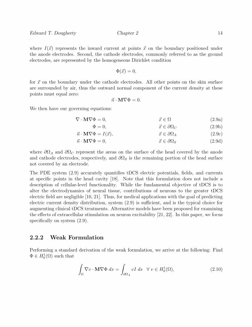
We then have our governing equations:
∇ ·M∇Φ = 0, ~x ∈ Ω (2.9a)
Φ = 0, ~x ∈ ∂ΩC (2.9b)
~n ·M∇Φ = I(~x), ~x ∈ ∂ΩA (2.9c)
~n ·M∇Φ = 0, ~x ∈ ∂ΩS (2.9d)
where ∂ΩA and ∂ΩC represent the areas on the surface of the head covered by the anodeand cathode electrodes, respectively, and ∂ΩS is the remaining portion of the head surfacenot covered by an electrode.
The PDE system (2.9) accurately quantifies tDCS electric potentials, fields, and currentsat specific points in the head cavity [18]. Note that this formulation does not include adescription of cellular-level functionality. While the fundamental objective of tDCS is toalter the electrodynamics of neural tissue, contributions of neurons to the greater tDCSelectric field are negligible [10, 21]. Thus, for medical applications with the goal of predictingelectric current density distribution, system (2.9) is sufficient, and is the typical choice foraugmenting clinical tDCS treatments. Alternative models have been proposed for examiningthe effects of extracellular stimulation on neuron excitability [21, 22]. In this paper, we focusspecifically on system (2.9).
2.2.2 Weak Formulation
Performing a standard derivation of the weak formulation, we arrive at the following: FindΦ ∈ H1
0 (Ω) such that ∫Ω
∇v ·M∇Φ dx =
∫∂ΩA
vI ds ∀ v ∈ H10 (Ω), (2.10)

Edward T. Dougherty Chapter 2 15
where
H10 (Ω) = u | u ∈ H1(Ω), u = 0 ∀ ~x ∈ ∂ΩC,
H1(Ω) = u | u ∈ L2(Ω),∂u
∂xi∈ L2(Ω), i = 1, ..., d,
and
L2(Ω) = p |∫
Ω
|p|2dx <∞.
2.2.3 Preconditioners
A finite element discretization of the weak formulation (2.10) generates a system of linearequations to be solved. This system can be represented in matrix-vector form as
Aij~φj = ~bi, i, j = 1, ..., n (2.11)
where the ith and jth entries are given by:
Aij =
∫Ω
∇Ni ·M∇Nj dx, bi =
∫∂ΩA
NiI ds,
and φj’s are the unknown scalar electric potentials that we are solving for over the discretizeddomain. Here, Ni, and Nj are basis functions over the discretized domain while n denotesthe number of basis functions in our discretization.
To simplify notation, for the remainder of this paper we will represent Aij simply as A.
A is symmetric and positive-definite, consequently the CG method is ideal in solving (2.11).However, this method alone does not necessarily produce acceptable results within reasonabletime constraints [15]. Convergence of the iterative solver can be significantly expedited withpreconditioning [23]. In the following subsections, we describe the preconditioners that areemployed in our tDCS simulations.
Jacobi
The Jacobi preconditioner approximates the coefficient matrix A with the diagonal entriesof A:
K = Aii.
SSOR
Our SSOR preconditioning approximates A as
K = (D + L)(D−1)(D + U), (2.12)

Edward T. Dougherty Chapter 2 16
where D is the diagonal of A, and L and U are the strictly lower and upper triangularmatrices of A [17].
Incomplete LU Factorizations (ILUs)
The ILU preconditioner is an incomplete LU factorization of a matrix [24] with the fill-indisregarded [16]:
K = L U,
where L and U are the LU factorization of A with the fill-in omitted.
Rather than completely disregarding the fill-in, the MILU (Modified ILU) preconditioneradds it into the main diagonal, and the RILU (Relaxed ILU) preconditioner incorporates afraction of the fill-in by a multiplicative weighting factor, ω ∈ [0, 1]. Note that when ω = 0or 1, we reattain the ILU and MILU preconditioners respectively [16]. For the remainder ofthis paper, “RILU” will be used to represent all incomplete LU factorization preconditioners,and RILU(ω) will denote RILU with a specific ω value. For example, RILU(0.7) representsthe RILU preconditioner with a relaxation parameter value of 0.7.
MG (Multigrid)
We refer to [25] for a detailed explanation of MG and provide just a brief overview of thealgorithm here as it relates to our tDCS numerical simulations. As its name implies, MGtakes advantage of multiple grid refinements to achieve highly accelerated convergence rates.The basic idea is to restrict and interpolate the residual ~r = ~bi −A~φj between coarser andfiner meshes respectively; by performing just a few iterations, and then changing from coarseto fine and vice versa, large portions of the error are efficiently removed.
Two commonly used sequences of restricting and interpolating, termed cycles, are typicallyused, namely the V-cycle and the W-cycle [25]. One of the challenges of MG is selectingappropriate and optimal parameter values. Several such parameters that must be specifiedinclude: (i) number of grid levels, (ii) grid cycle type, (iii) pre and post smoothing iterativesolvers, (iv) coarse grid iterative solver, and (v) number of pre-smooth, post-smooth andcoarse grid iterations to perform [17].
2.3 Methods
2.3.1 Computational Tools
Our tDCS numerical simulations were performed on three-dimensional volume meshes gen-erated from human MRI images. These meshes are provided by the SimNIBS software

Edward T. Dougherty Chapter 2 17
package [13], and possess quality tetrahedral meshes of the skin, skull, CSF, GM, and WMportions of the head. Mesh visualization was accomplished with Gmsh [26] and then ex-ported to a grid file format supported by Diffpack1 [27]. Figure (2.1) displays portions ofthe computational meshes used in our tDCS simulations.
(a) Head mesh used in tDCS simulations (b) WM and GM portion of mesh used in tDCSsimulations
Figure 2.1 Portions of computational meshes used in tDCS numerical simulations.
Finite element solutions were performed with Diffpack, which involved implementing theweak formulation (2.10) of the PDE system (2.9), as well as the boundary conditions de-termined by the different electrode montages presented in section 2.3.2. The CG method,MG, and all preconditioners analyzed (see section 2.2.3) are supported by Diffpack. Con-vergence histories for each numerical experiment were archived and then visualized withgnuplot2. Voltage and electric field results were exported to VTK format and visualizedwith ParaView3.
2.3.2 Electrode Montages
Three separate electrode montages were selected for our tDCS numerical experiments (seeTable 2.1). Each montage has been used in multiple tDCS medical experiments. Collectively,these configurations encompass a wide range of tDCS treatment applications. In addition,they provide diverse boundary conditions which yield diverse numerical experiments. Eachmontage is specified using the international 10-20 system [28].
1www.diffpack.com2www.gnuplot.info3www.paraview.org

Edward T. Dougherty Chapter 2 18
Table 2.1 tDCS numerical experiment electrode positions with associated medical applica-tions. Electrode locations are specified using the international 10-20 system.
Anode Cathode(s) Medical Applications
Montage 1 C3 C4 Motor sequence learning [29]Post-stroke physical therapy [7]
Montage 2 Forehead symmetric Mastoids (both) Parkinson’s disease [1, 11]
Montage 3 C3 Fp2 Post-stroke recovery [6]Chronic pain management [5]
2.3.3 tDCS Numerical Experiments
Numerical simulations were executed on three different mesh refinements:Approximately 5.2 million (M) elements (with roughly 914,000 unknowns), which we willrefer to as “grid-5M”,approximately 16.0 M elements (with roughly 2.8 M unknowns), referred to as “grid-16M”,andapproximately 28.9 M elements (with roughly 5.1 M unknowns), referred to as “grid-28M”.
The first set of numerical experiments were conducted to evaluate the convergence per-formance of the preconditioned conjugate gradient method. For each montage, we executedtDCS simulations with the CG method preconditioned with the following strategies:
1. No preconditioning
2. Jacobi
3. SSOR
4. RILU: ω = 0.0, 0.1, 0.2, 0.3, 0.4, 0.5, 0.6, 0.7, 0.8, 0.9, and 1.0.
5. MG: Standard 2 grid V-cycle with 1 SSOR iteration for pre and post smoothing anda maximum of 20 SSOR iterations for coarse grid solving.
All preconditioners were tested with grid-5M and grid-16M. Based on these results, thosepreconditioners with reasonable convergence performance were then tested on grid-28M.
The second set of experiments test MG as a stand-alone iterative solver. The same param-eter values as the MG preconditioner were used, and we evaluated this method with eachof the three electrode montages on grid-5M. As will be shown in section 2.4.4, this methodhad poor convergence results. To identify reasons for this, numerical experiments with dif-ferent boundary conditions for (2.9a) and homogeneous tissue conductivities were conducted.

Edward T. Dougherty Chapter 2 19
Finally, we analyze the influence of different MG preconditioner parameter values on theconvergence performance of the CG method. To do so, we simulated each montage on grid-28M with three grid levels, grid-28M being the finest, with all combinations of the followingparameter values:
1. Grid cycle: V and W
2. SSOR iteration maximums for coarse grid solving: 10 and 20
In total, 120 tDCS numerical simulations were performed.
A relative residual convergence monitor, namely ‖rk‖‖r0‖ was used, where ‖r0‖ is the norm of
the initial residual, and ‖rk‖ is the norm of the residual of the kth iteration. Convergencetolerance was set to 10−8 for all numerical experiment. Additionally, linear tetrahedralfinite element basis functions were used on all grids. Convergence performance is assessedby the number of iterations to numerical convergence and CPU linear system solve time;for benchmark consistency, all simulations were run on a Linux machine with an Intel i7processor with a clock speed of 2.40 GHz.
Electrical conductivities were assigned to different tissues: skin = 0.465, skull = 0.010, CSF= 1.654, GM = 0.276, and WM = 0.126, each with units S
m[30]. Anode electric current was
set to 1 mA (2.9c), and the surface area of each electrode is approximately 25 cm2 [1, 29].
2.4 Results
2.4.1 Montage 1- conjugate gradient method
Electric potential and electric current density results on the surface of the head are displayedin Figs. 2.2a and 2.2b. Viewing perspective is from directly above the head with the nasionfacing down. As expected in a passive volume conductor, maximum and minimum voltagesand current magnitudes coincide with electrode placement.
Figure 2.2c displays a cross-section of the head taken through a plane intersecting the C3anode and C4 cathode electrodes, viewed from the anterior. A significant portion of theelectric current shunts around the skull due to its low conductivity [10]. The curvilinearelectric field lines result from the interwoven, juxtaposed CSF, GM and WM. The portion ofthe electric current that immediately diverts at the anode results in the segregated, patch-likeformation at this location (Fig. 2.2b). The inner portion of the magnitude is approximately1.0 mA, the specified anode current value. The diversion of the electric current along theskull increases the magnitude of the current density parallel to the anode, which forms ahigher magnitude region (>1.3 mA) that surrounds the inner segment. The tendency of the

Edward T. Dougherty Chapter 2 20
(a) Electric potential on headsurface
(b) Electric current density onhead surface
(c) Electric current density andfield stream lines from cross-sectionthrough the anode and cathode elec-trode centres, viewing perspective isanterior
Figure 2.2 Montage 1 finite element solution results.
electric current to circumscribe the cerebral volume lends its exit towards the edges of thecathode. This is illustrated by the near zero current magnitude at the center of the cathode,and maximal values at its edges (Fig. 2.2b).
Table 2.2 and Fig. 2.3 display the convergence performance and history of each precondi-tioning strategy on all three grid refinements for montage 1. With no preconditioning, theCG method will eventually converge, but does so very slowly (>2,000 iterations). Jacobipreconditioning is also noticeably inferior with much higher iteration counts and computetimes. RILU (0.7) produces the fastest convergence of all ω examined (see section 2.2.3)on both grid-5M and grid-16M, converging in 480 and 666 iterations respectively. SSORperformance is near identical to RILU(0.7) on grid-5M with 488 iterations, but is 5.25%higher than RILU(0.7) on grid-16M with 701 iterations. SSOR converges in fewer itera-tions than what was achieved with four values of ω, namely RILU(0.0, 0.1, 0.9, and 1.0),demonstrating the importance of screening RILU relaxation parameter values, and the de-pendence of the RILU preconditioner on this parameter. On grid-5M, the conjugate gradientmethod preconditioned with MG converges in the fewest iterations and the least computetime. However on both grid-16M and grid-28M, despite having by far the fewest iterations,MG preconditioning has a more expensive run time.
2.4.2 Montage 2- conjugate gradient method
Surface electric potential and electric current results for the second electrode montage ispresented in Fig. 2.4. The cathode over the patient’s left mastoid is shown (Fig. 2.4b), and

Edward T. Dougherty Chapter 2 21
Table 2.2 Convergence performance of the conjugate gradient method with the montage 1electrode configuration. Boldface values indicate best convergences within the grid.
Iterations and Solve Time (min)Preconditioner grid-5M grid-16M grid-28M
None > 2000 22.5 > 2000 74.8 — —Jacobi 1203 14.3 1731 67.1 — —SSOR 488 10.4 701 51.3 869 117.8RILU 480 10.9 666 47.1 884 122.2MG 115 10.3 177 51.2 217 131.3
-9
-8
-7
-6
-5
-4
-3
-2
-1
0
1
0 200 400 600 800 1000 1200 1400 1600 1800 2000
log
10
(Re
lative
Re
sid
ua
l)
Iterations
None
Jacobi
SSOR
RILU
Multigrid
(a) grid-5M
-9
-8
-7
-6
-5
-4
-3
-2
-1
0
1
0 200 400 600 800 1000 1200 1400 1600 1800 2000
log
10
(Re
lative
Re
sid
ua
l)
Iterations
None
Jacobi
SSOR
RILU
Multigrid
(b) grid-16M
-9
-8
-7
-6
-5
-4
-3
-2
-1
0
1
0 200 400 600 800 1000
log
10
(Re
lative
Re
sid
ua
l)
Iterations
SSOR
RILU
Multigrid
(c) grid-28M
Figure 2.3 Montage 1 convergence history of the preconditioned conjugate gradient method.
although not visible an identical cathode is positioned over the right mastoid area. Maximumvoltage occurs under the anode center (Fig. 2.4a). The electric current density and fielddirection is shown via a cross-section through the anode and left mastoid cathode. Viewingperspective is from the left side, with the head facing towards the left. A portion of theelectric current can be seen shunting along the skull (Fig. 2.4c) as observed in montage 1,and a similar inner and outer segmentation of the current density is formed at the anodeand cathodes. Wave-like electric field lines through the interwoven CSF, GM, and WM arealso visible.
Table 2.3 and Fig. 2.5 display the convergence performance and history for montage 2. TheCG method again converges very slowly with no preconditioning and Jacobi preconditioning.For the RILU preconditioner, relaxation parameter values of ω=0.5, 0.6, and 0.7 producethe best convergence rates on grid-5M, and RILU(0.7) was superior on grid-16M. RILU(1.0)causes the CG method to not converge within 2,000 iterations on both grid-5M and grid-16M. SSOR converges the fastest on grid-5M and grid-28M. Excluding RILU(1.0), SSORhad lower iteration counts than only RILU(0.9) on grid-5M, which needed 480 iterations forconvergence. Further, SSOR does not outperform any RILU preconditioner in iteration countor execution time on grid-16M, again excluding RILU (1.0). Once again, CG preconditionedwith MG produced by far the lowest iteration count, but offers no advantage in simulation

Edward T. Dougherty Chapter 2 22
(a) Electric potential on headsurface from anode
(b) Electric potential on head surfacefrom cathode over left mastoid
(c) Electric current density and fieldstream lines taken through a planeintersecting the anode and cathodeover left mastoid cathode
Figure 2.4 Montage 2 finite element solution results.
execution time.
Table 2.3 Convergence performance of the conjugate gradient method with the montage 2electrode configuration. Boldface values indicate best convergences within the grid.
Iterations and Solve Time (min)Preconditioner grid-5M grid-16M grid-28M
None > 2000 22.7 > 2000 74.9 — —Jacobi 1142 13.6 1658 64.3 — —SSOR 467 9.7 668 49.1 832 113.1RILU 459 10.5 630 44.6 847 117.5MG 111 9.8 171 50.7 211 128.7
The electrode placement of montage 2 is substantially different than montage 1; anode place-ment differs by approximately 25% along the scalp circumference, and montage 2 has twocathodes positioned at the lower sides of the head as opposed to the one cathode at the topof the head in montage 1. Despite these dissimilar electrode configurations, preconditionerperformances are quite similar; increases in iterations and execution times of the Jacobi,SSOR, RILU and MG preconditioners across grid refinements are relatively comparable be-tween these montages. In addition, MG has almost identical iteration counts and simulationtimes in both montages.
2.4.3 Montage 3- conjugate gradient method
Finite element results of the surface potential and electric current density, as well as theelectric field lines are shown in Fig. 2.6. Field lines (Fig. 2.6c) are shown in a cross-section

Edward T. Dougherty Chapter 2 23
-9
-8
-7
-6
-5
-4
-3
-2
-1
0
1
0 200 400 600 800 1000 1200 1400 1600 1800 2000
log
10
(Re
lative
Re
sid
ua
l)
Iterations
None
Jacobi
SSOR
RILU
Multigrid
(a) grid-5M
-9
-8
-7
-6
-5
-4
-3
-2
-1
0
1
0 200 400 600 800 1000 1200 1400 1600 1800 2000
log
10
(Re
lative
Re
sid
ua
l)
Iterations
None
Jacobi
SSOR
RILU
Multigrid
(b) grid-16M
-9
-8
-7
-6
-5
-4
-3
-2
-1
0
1
0 200 400 600 800 1000
log
10
(Re
lative
Re
sid
ua
l)
Iterations
SSOR
RILU
Multigrid
(c) grid-28M
Figure 2.5 Montage 2 convergence history of the preconditioned conjugate gradient method.
through the anode and cathode electrodes, viewed from the patient’s left. A similar currentdensity partitioning under the anode and cathode is seen, as well as skull-divergent andconvoluted cerebral electric field lines.
(a) Electric potential on head sur-face
(b) Electric current density on headsurface
(c) Electric current density andfield stream lines from cross-sectiontaken through a plane intersectingthe C3 anode and Fp2 cathode
Figure 2.6 Montage 3 finite element solution results.
Table 2.4 and Fig. 2.7 display the convergence performance of each preconditioning strategyfor montage 3, and similar results are observed. No preconditioning and Jacobi precondition-ing yields poor convergence behavior. Multigrid produces the lowest iteration counts, yetwith longer computing times. On grid-5M, RILU(0.5) and RILU(0.6) produce the fastestconvergence rates with 476 iterations, followed closely by RILU(0.7) with 477 iterations,and the fastest execution time. SSOR performance is similar to RILU(0.5, 0.6, and 0.7) ongrid-5M, and requires fewer iterations than all RILU preconditioners, yet its performancedeteriorates faster than RILU when moving to grid-16M, but again offers superior perfor-mance to the RILU preconditioners on grid-28M. Once again, MG iteration counts are by

Edward T. Dougherty Chapter 2 24
far the lowest, but execution times offer no advantage.
Table 2.4 Convergence performance of the conjugate gradient method with the montage 3electrode configuration. Boldface values indicate best convergences within the grid.
Iterations and Solve Time (min)Preconditioner grid-5M grid-16M grid-28M
None > 2000 24.3 > 2000 74.6 — —Jacobi 1172 15.0 1706 68.8 — —SSOR 475 11.0 695 50.2 846 115.7RILU 476 10.2 655 43.4 873 122.2MG 116 10.4 177 49.2 219 132.7
-9
-8
-7
-6
-5
-4
-3
-2
-1
0
1
0 200 400 600 800 1000 1200 1400 1600 1800 2000
log
10
(Re
lative
Re
sid
ua
l)
Iterations
None
Jacobi
SSOR
RILU
Multigrid
(a) grid-5M
-9
-8
-7
-6
-5
-4
-3
-2
-1
0
1
0 200 400 600 800 1000 1200 1400 1600 1800 2000
log
10
(Re
lative
Re
sid
ua
l)
Iterations
None
Jacobi
SSOR
RILU
Multigrid
(b) grid-16M
-9
-8
-7
-6
-5
-4
-3
-2
-1
0
1
0 200 400 600 800 1000
log
10
(Re
lative
Re
sid
ua
l)
Iterations
SSOR
RILU
Multigrid
(c) grid-28M
Figure 2.7 Montage 3 convergence history of the preconditioned conjugate gradient method.
The electrode placement of montage 3 is similar to montage 1 in that both montages havethe anode located at C3; common solver performance between these two montages was notunexpected. Montage 3, however, is substantially different than montage 2. First, the anodeplacement in montage 2 (center forehead) is very close to the cathode placement in montage3 (Fp2 contralateral supraorbital). Second, the cathodes positioned over the mastoids inmontage 2 are virtually as distant from the Fp2 cathode as possible in tDCS. Yet we againsee very similar convergence results across all three montages, suggesting that montageconfiguration does not substantially impact iterative method performance.
2.4.4 Multigrid as a stand-alone iterative method
MG as a stand-alone iterative method has shown success in solving the classical Poissonequation [31]; equation (2.9a) is the homogeneous form of the Poisson equation with spatially-dependent conductivities. In our experiments, however, MG as an iterative solver diverges ongrid-5M on all three montages. Two main properties of tDCS simulations that are potentialcontributors to the divergence are: (i) the tDCS inhomogeneous tissue conductivities [17]

Edward T. Dougherty Chapter 2 25
and (ii) the collection of mixed homogeneous and inhomogeneous boundary conditions (2.9b,2.9c, 2.9d).
To determine the influence of each of these properties, we ran the following experiments ongrid-5M:
1. Test the influence of just inhomogeneous conductivities:Equation (2.9a) with boundary conditions (2.9b - 2.9d) unchanged, but with a homo-geneous conductivity throughout the entire domain: M = 0.5, ~x ∈ Ω.
2. Test the influence of just boundary conditions:Equation (2.9a) with the tDCS inhomogeneous tissue conductivities defined in section2.3.3, but with a single Dirichlet boundary condition on the entire boundary: Φ(~x) =1.0, ~x ∈ ∂Ω.
3. Test the influence of both inhomogeneous conductivities AND boundary conditions:Homogeneous conductivity M = 0.5, ~x ∈ Ω, and Dirichlet boundary condition: Φ(~x) =1.0, ~x ∈ ∂Ω.
For the first and second experiments, MG as a stand-alone solver still diverges on all threemontages. However, MG did converge on the third experiment on all three montages. Theseresults suggest that either the tDCS inhomogeneous conductivities or the mixed boundaryconditions (2.9b, 2.9c, 2.9d) cause the MG iterative solver to diverge.
Observations of MG diverging when solving the Poisson equation due to “jumping” conduc-tivities is well documented [17] [20]. The most drastic tissue interface conductivity disconti-nuity in our simulations is between the skull and CSF, where the conductivity of the CSF is165 times that of the skull. Given the multiple and vastly different conductivities in tDCSsimulations, the divergent behavior of MG a a stand-alone method is not unexpected.
2.4.5 Parameter influence- conjugate gradient preconditioned withmultigrid
In the previous simulations, the CG method preconditioned with MG offered a dramaticreduction in iteration counts compared to the other preconditioning strategies, yet no sub-stantial gain in overall execution times were observed. The performance of a multigrid pre-conditioner is highly sensitive to its parameter settings. This last series of tDCS numericalexperiments was conducted to evaluate the convergence performance of CG preconditionedwith MG, with different MG parameter values in an attempt to achieve faster convergencerates. We examined the following three parameters: (i) number of grid levels, (ii) cycle type,and (iii) coarse grid solver iterations. These three MG parameters have demonstrated greatimpact on CG convergence performance [17].

Edward T. Dougherty Chapter 2 26
To assess the influence of these settings, we simulated each of the three montages on grid-28Mwith 3 grid levels, with all combinations of the following parameter values:
1. V and W cycles
2. 10 and 20 SSOR iteration maximums for coarse grid solving
Other MG parameters were kept the same, i.e. 1 SSOR iteration for pre and post smoothing(see section 2.3.3).
Table 2.5 and Fig. 2.8 display the convergence results for these experiments. The conver-gence values and curves for the 2 grid V-cycle are replicated from our previous results todemonstrate the effect of the new parameter settings.
Table 2.5 Convergence performance of the conjugate gradient method with different multi-grid preconditioner parameter settings on grid-28M. Boldface values indicate best conver-gences for each montage.
MG Params Iterations and Solve Time (min)Num Grids Cycle SSOR Iters Montage 1 Montage 2 Montage 3
2 grid V 10 217 131.3 211 128.7 219 132.73 grid V 10 138 64.1 134 62.5 138 61.63 grid V 20 118 58.1 112 54.8 116 55.33 grid W 10 120 65.6 113 61.8 117 61.03 grid W 20 110 65.4 104 61.2 108 63.6
-9
-8
-7
-6
-5
-4
-3
-2
-1
0
1
0 50 100 150 200 250
log
10
(Re
lative
Re
sid
ua
l)
Iterations
2 grid, V cycle, 10 SSOR iters
3 grid, V cycle, 10 SSOR iters
3 grid, V cycle, 20 SSOR iters
3 grid, W cycle, 10 SSOR iters
3 grid, W cycle, 20 SSOR iters
(a) Montage 1
-9
-8
-7
-6
-5
-4
-3
-2
-1
0
1
0 50 100 150 200 250
log
10
(Re
lative
Re
sid
ua
l)
Iterations
2 grid, V cycle, 10 SSOR iters
3 grid, V cycle, 10 SSOR iters
3 grid, V cycle, 20 SSOR iters
3 grid, W cycle, 10 SSOR iters
3 grid, W cycle, 20 SSOR iters
(b) Montage 2
-9
-8
-7
-6
-5
-4
-3
-2
-1
0
1
0 50 100 150 200 250
log
10
(Re
lative
Re
sid
ua
l)
Iterations
2 grid, V cycle, 10 SSOR iters
3 grid, V cycle, 10 SSOR iters
3 grid, V cycle, 20 SSOR iters
3 grid, W cycle, 10 SSOR iters
3 grid, W cycle, 20 SSOR iters
(c) Montage 3
Figure 2.8 Convergence history of the conjugate gradient method preconditioned withdifferent multigrid parameter settings on grid-28M.
In all three montages, there are significant performance enhancements just by increasing thenumber of MG grids from two to three. In montage 1, for example, the iteration count dropsfrom 217 to 138, and run time is decreased by more than half. Similar findings are seen in
Edward T. Dougherty Chapter 2 27
montages 2 and 3. More remarkable improvements in iterations and run time are seen whenincreasing the number of V-cycle maximum coarse grid iterations from 10 to 20.
The conjugate gradient method preconditioned with a multigrid W-cycle demonstrates sim-ilar execution times for 10 or 20 maximum coarse grid iterations. In addition, multigridW-cycle preconditioning has fewer iterations than its V-cycle sibling, however, its executiontimes offer no significant improvement. Fastest convergence times are seen when using a 3grid, V-cycle with a maximum of 20 SSOR iterations. These times are also far superior tothose attained by the SSOR and RILU preconditioners seen in sections 2.4.1, 2.4.2, and 2.4.3.In addition, similar performances and improvements across each montage is again observed,reinforcing the notion that the performance of the iterative method is not substantiallydependent on tDCS electrode placement.
2.5 Conclusions and further work
We have presented a comprehensive comparison of iterative solver strategies for tDCS sim-ulations. Using several grid refinements and tDCS montage arrangements, the CG methodfor solving the finite element discretized system of equations was evaluated with a range ofpreconditioners, as well as MG as a standalone iterative solver. Of all methods examined, theCG method preconditioned with an appropriately configured multigrid algorithm producedsuperior convergence rates.
We found that different tDCS montages yield very similar convergence histories despite vastdifferences in electrode configurations. As a stand-alone iterative solver, MG diverges on allelectrode montages examined due to the inhomogeneous tissue conductivities and boundarycondition conglomerate. In addition, MG as a preconditioner with inappropriate parametervalues yields convergence results no better, and at times worse than simpler preconditioningschemes, e.g. SSOR and RILU.
Our finite element solution visualizations showcase the curvilinear nature of electric fieldlines within the cerebral region. An inner-outer pattern of electric current at the anodedue to divergence along the skull was observed. In addition, this field’s circuitous tendencyfacilitates an arrival of current at the edges of the cathode. Other tDCS simulations havedemonstrated similar behavior [11]. This phenomena is highlighted and quite visible in oursimulations given the fine mesh resolutions utilized.
Our primary objective in this work was to identify computationally efficient iterative solutionapproaches for real-world tDCS simulations from the medical view-point, namely simulationsthat incorporate treatment-based electrode arrangements on MRI-derived three-dimensionalhead models, and physiologically-based inhomogeneous tissue conductivities. In future work,we plan to analyze tDCS solution methods from the numerics perspective. In particular, weplan to estimate solution rates of convergence and numerically analyze MG preconditioningin a tDCS context. Further, we would like to investigate other MG performance influences,

Edward T. Dougherty Chapter 2 28
including alternative grid cycles such as full MG, and different pre-sweep and post-sweep it-erations. We also intend to examine the influence of isotropic and anisotropic tissue conduc-tivity representations on the performance of different preconditioners and iterative methods.
2.6 Acknowledgements
We would like to thank Tobias Wittner of inuTech GmbH for his assistance with Diffpackand Multigrid software support.
2.7 Bibliography
[1] D. H. Benninger, M. Lomarev, G. Lopez, E. M. Wassermann, X. Li, E. Considine, andM. Hallett. Transcranial direct current stimulation for the treatment of Parkinson’sdisease. J. Neurol. Neurosurg. Psychiatr., 81(10):1105–1111, Oct 2010.
[2] P. S. Boggio, R. Ferrucci, S. P. Rigonatti, P. Covre, M. Nitsche, A. Pascual-Leone,and F. Fregni. Effects of transcranial direct current stimulation on working memory inpatients with Parkinson’s disease. J. Neurol. Sci., 249(1):31–38, Nov 2006.
[3] P. S. Boggio, L. P. Khoury, D. C. Martins, O. E. Martins, E. C. de Macedo, andF. Fregni. Temporal cortex direct current stimulation enhances performance on a vi-sual recognition memory task in Alzheimer disease. J. Neurol. Neurosurg. Psychiatr.,80(4):444–447, Apr 2009.
[4] P. S. Boggio, C. A. Valasek, C. Campanha, A. C. Giglio, N. I. Baptista, O. M. Lapenta,and F. Fregni. Non-invasive brain stimulation to assess and modulate neuroplasticityin Alzheimer’s disease. Neuropsychol Rehabil, 21(5):703–716, Oct 2011.
[5] A. F. DaSilva, M. S. Volz, M. Bikson, and F. Fregni. Electrode positioning and montagein transcranial direct current stimulation. J Vis Exp, (51), 2011.
[6] G. Schlaug, V. Renga, and D. Nair. Transcranial direct current stimulation in strokerecovery. Arch. Neurol., 65(12):1571–1576, Dec 2008.
[7] S. Hesse, A. Waldner, J. Mehrholz, C. Tomelleri, M. Pohl, and C. Werner. Com-bined transcranial direct current stimulation and robot-assisted arm training in suba-cute stroke patients: an exploratory, randomized multicenter trial. Neurorehabil NeuralRepair, 25(9):838–846, 2011.
[8] T. Neuling, S. Wagner, C. H. Wolters, T. Zaehle, and C. S. Herrmann. Finite-ElementModel Predicts Current Density Distribution for Clinical Applications of tDCS andtACS. Front Psychiatry, 3:83, 2012.

Edward T. Dougherty Chapter 2 29
[9] F. Gasca, L. Marshall, S. Binder, A. Schlaefer, U.G. Hofmann, and A. Schweikard. Finiteelement simulation of transcranial current stimulation in realistic rat head model. InNeural Engineering (NER), 2011 5th International IEEE/EMBS Conference on, pages36–39, April 2011.
[10] A. Datta, X. Zhou, Y. Su, L. C. Parra, and M. Bikson. Validation of finite element modelof transcranial electrical stimulation using scalp potentials: implications for clinical dose.J Neural Eng, 10(3):036018, Jun 2013.
[11] P. C. Miranda, M. Lomarev, and M. Hallett. Modeling the current distribution duringtranscranial direct current stimulation. Clin Neurophysiol, 117(7):1623–1629, Jul 2006.
[12] S. K. Kessler, P. Minhas, A. J. Woods, A. Rosen, C. Gorman, and M. Bikson. Dosageconsiderations for transcranial direct current stimulation in children: a computationalmodeling study. PLoS ONE, 8(9):e76112, 2013.
[13] Mirko Windhoff, Alexander Opitz, and Axel Thielscher. Electric field calculations inbrain stimulation based on finite elements: An optimized processing pipeline for thegeneration and usage of accurate individual head models. Human Brain Mapping,34(4):923–935, 2013.
[14] S. Lew, C. H. Wolters, T. Dierkes, C. Roer, and R. S. Macleod. Accuracy and run-time comparison for different potential approaches and iterative solvers in finite elementmethod based EEG source analysis. Appl Numer Math, 59(8):1970–1988, Aug 2009.
[15] H.A. van der Vorst. Iterative Krylov Methods for Large Linear Systems. Cambridgemonographs on applied and computational mathematics. Cambridge University Press,2003.
[16] H. P. Langtangen. Computational Partial Differential Equations: Numerical Methodsand Diffpack Programming. Texts in Computational Science and Engineering. SpringerBerlin Heidelberg, 2003.
[17] K. A. Mardal, G. W. Zumbusch, and H. P. Langtangen. Software tools for multigridmethods. In H. P. Langtangen and A. Tveito, editors, Advanced Topics in Compu-tational Partial Differential Equations:Numerical Methods and Diffpack Programming,Lecture Notes in Computational Science and Engineering, pages 97–152. Springer BerlinHeidelberg, 2003.
[18] Robert Plonsey and DennisB. Heppner. Considerations of quasi-stationarity in electro-physiological systems. The bulletin of mathematical biophysics, 29(4):657–664, 1967.
[19] J. Sundes, G. T. Lines, P. Grottum, and A. Tveito. Electrical activity in the humanheart. In H. P. Langtangen and A. Tveito, editors, Advanced Topics in ComputationalPartial Differential Equations:Numerical Methods and Diffpack Programming, Lecture

Edward T. Dougherty Chapter 2 30
Notes in Computational Science and Engineering, pages 402–449. Springer Berlin Hei-delberg, 2003.
[20] J. Sundnes, G. T. Lines, X. Cai, F. N. Bjorn, K. A. Mardal, and A. Tveito. Computingthe electrical activity in the heart. Springer, Berlin New York, 2006.
[21] E. Dougherty, J. Turner, and F. Vogel. Multiscale Coupling of Transcranial DirectCurrent Stimulation to Neuron Electrodynamics: Modeling the Influence of the Tran-scranial Electric Field on Neuronal Depolarization. Computational and MathematicalMethods in Medicine, 2014(Article ID 360179):1–14, 2014.
[22] R. Szmurlo, J. Starzynski, S. Stanislaw, and A. Rysz. Numerical model of vagus nerveelectrical stimulation. The International Journal for Computation and Mathematics inElectrical and Electronic Engineering, 28(1):211–220, 2009.
[23] K. A. Mardal, J. Sundes, H. P. Langtangen, and A. Tveito. Systems of pdes andblock preconditioning. In H. P. Langtangen and A. Tveito, editors, Advanced Topicsin Computational Partial Differential Equations:Numerical Methods and Diffpack Pro-gramming, Lecture Notes in Computational Science and Engineering, pages 200–236.Springer Berlin Heidelberg, 2003.
[24] Y Saad. Iterative methods for sparse linear systems. PWS Pub. Co, Boston, 1996.
[25] William Briggs. A multigrid tutorial. Society for Industrial and Applied Mathematics,Philadelphia, PA, 2000.
[26] Christophe Geuzaine and Jean-Franois Remacle. Gmsh: A 3-d finite element meshgenerator with built-in pre- and post-processing facilities. International Journal forNumerical Methods in Engineering, 79(11):1309–1331, 2009.
[27] Are Magnus Bruaset and Hans Petter Langtangen. Diffpack: A software environmentfor rapid protoptying of pde solvers.
[28] M. A. Nitsche, L. G. Cohen, E. M. Wassermann, A. Priori, N. Lang, A. Antal,W. Paulus, F. Hummel, P. S. Boggio, F. Fregni, and A. Pascual-Leone. Transcra-nial direct current stimulation: State of the art 2008. Brain Stimul, 1(3):206–223, Jul2008.
[29] E. K. Kang and N. J. Paik. Effect of a tDCS electrode montage on implicit motorsequence learning in healthy subjects. Exp Transl Stroke Med, 3(1):4, 2011.
[30] A. Datta, J. M. Baker, M. Bikson, and J. Fridriksson. Individualized model predictsbrain current flow during transcranial direct-current stimulation treatment in responsivestroke patient. Brain Stimul, 4(3):169–174, Jul 2011.

Edward T. Dougherty Chapter 2 31
[31] H. P. Langtangen and A. Tveito. Advanced Topics in Computational Partial Differ-ential Equations: Numerical Methods and Diffpack Programming. Lecture Notes inComputational Science and Engineering. Springer Berlin Heidelberg, 2003.

Chapter 3
An Object-Oriented Framework forVersatile Finite Element BasedSimulations of Neurostimulation
Edward Dougherty and James Turner
32

Edward T. Dougherty Chapter 3 33
Abstract
Objective. Computational simulations of transcranial electrical stimulation (TES) are com-monly utilized by the neurostimulation community, and while vastly different TES applica-tion areas can be investigated, the mathematical equations and physiological characteristicsthat govern this research are identical. The goal of this work was to develop a robust softwareframework for TES that efficiently supports the spectrum of computational simulations rou-tinely utilized by the TES community, and in addition, easily extends to support alternativeneurostimulation research objectives.
Approach. Using well-established object-oriented software engineering techniques, we havedesigned a software framework based upon the physical and computational aspects of TES.General neurostimulation concepts have been encapsulated into modular software compo-nents, and integrated into a single computer code. The framework’s versatility is demon-strated with a set of diverse TES simulations. Finally, we show how the framework can beextended to support different forms of neurostimulation.
Main results. This paper presents a software framework that efficiently supports the broadrange of TES computational simulations. Simulations carried out by the framework (i)reinforce the importance of using anisotropic tissue conductivities, (ii) demonstrate the en-hanced precision of high-definition stimulation electrodes, and (iii) highlight the benefits ofutilizing multigrid solution algorithms. Finally, results show that tissue conductivity rep-resentation impacts deep brain stimulation electrical current dispersion simulation results,further stressing the necessity of incorporating anisotropic conductivity data to ensure ac-curate computational simulations.
Significance. This paper provides the first software design and implementation that sup-ports highly-versatile neurostimulation simulations. Our approach results in a frameworkthat facilitates rapid prototyping of real-world, customized TES administrations, and sup-ports virtually any clinical, biomedical, or computational aspect of this treatment. Softwarereuse and maintainability is optimized, and in addition, the same code can be effortlesslyaugmented to provide support for alternative neurostimulation research endeavours.

Edward T. Dougherty Chapter 3 34
3.1 Introduction
Transcranial electrical stimulation (TES) is a collection of non-invasive neurostimulationtechniques that strategically modulate activity in regions of the brain with low magnitudeelectric current delivered through electrodes positioned on the scalp surface. Forms of TESinclude the commonly used transcranial direct current stimulation (tDCS), as well as tran-scranial alternating current stimulation (tACS) [1]. Recently, the use of numerous smallersized electrodes, termed high-definition tDCS (HD-tDCS), has emerged as a form of TESthat enhances electrical current focality [2, 3]. Clinical and biomedical research continue todemonstrate the capabilities of TES as a medical treatment. For example, Alzheimer andParkinson’s disease patients have demonstrated increased memory abilities [4–6]. In addi-tion, TES has shown to alleviate symptoms of psychiatric disorders including depression [7, 8]and schizophrenia [9–11].
The efficacy and comprehension of TES has been enhanced with mathematical modelingand computational simulation. In particular, simulations can compute the current densitydistribution for a given patient and TES apparatus configuration [1, 12–15], and have demon-strated the importance of modulating treatment stimulation dosage [16]. Other simulationshave illustrated the importance of incorporating anisotropic tissue conductivity data [17, 18],and numerical studies aid in identifying the computational solution methods most efficientin simulating TES mathematical models [19, 20].
Object-oriented design is a software design approach that defines objects, which are sim-ply software entities that encapsulate data and functionality, and the relationships amongobjects. Features of object-oriented design can be utilized to maximize code re-usability,simplify software maintenance, and promote application versatility [21]. The prevalence ofobject-oriented design in scientific and biomedical applications began in the 1990s, and itsuse has dramatically increased due to its advantages over procedural software implementa-tions [22–27]. In particular, mathematical and physical attributes of a model can be naturallyrepresented with objects [28, 29].
A common approach for simulating partial differential equation (PDE) based mathematicalmodels is to use pre-built simulation software programs. These “black-boxes” can simplifymodel implementation, however, there are limitations with this approach. A researcher isoften confined to the numerical algorithms and programming controls offered by the sim-ulation program; it can be very difficult, or perhaps not possible, to incorporate numericsand solution techniques not supported by the software. In addition, integrating a pre-builtsoftware application with external data sources and applications can be very challenging,which obstructs the use of its simulations within larger software solutions.
An alternative strategy is to create custom software that utilizes numerical application pro-gramming interfaces (APIs). While this approach generally takes longer to implement, itallows the use of problem-specific algorithms and programming logic that facilitate accurateand expedient simulation results [29]. Coupling this philosophy with object-oriented soft-
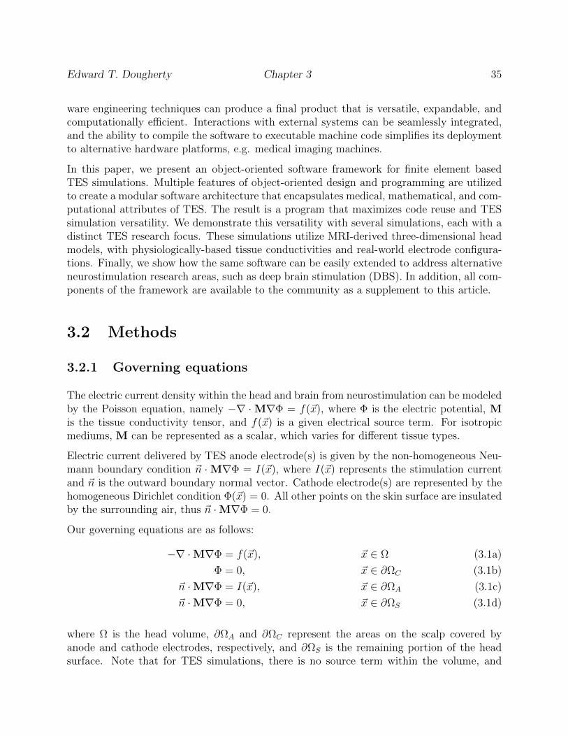
Edward T. Dougherty Chapter 3 35
ware engineering techniques can produce a final product that is versatile, expandable, andcomputationally efficient. Interactions with external systems can be seamlessly integrated,and the ability to compile the software to executable machine code simplifies its deploymentto alternative hardware platforms, e.g. medical imaging machines.
In this paper, we present an object-oriented software framework for finite element basedTES simulations. Multiple features of object-oriented design and programming are utilizedto create a modular software architecture that encapsulates medical, mathematical, and com-putational attributes of TES. The result is a program that maximizes code reuse and TESsimulation versatility. We demonstrate this versatility with several simulations, each with adistinct TES research focus. These simulations utilize MRI-derived three-dimensional headmodels, with physiologically-based tissue conductivities and real-world electrode configura-tions. Finally, we show how the same software can be easily extended to address alternativeneurostimulation research areas, such as deep brain stimulation (DBS). In addition, all com-ponents of the framework are available to the community as a supplement to this article.
3.2 Methods
3.2.1 Governing equations
The electric current density within the head and brain from neurostimulation can be modeledby the Poisson equation, namely −∇ ·M∇Φ = f(~x), where Φ is the electric potential, Mis the tissue conductivity tensor, and f(~x) is a given electrical source term. For isotropicmediums, M can be represented as a scalar, which varies for different tissue types.
Electric current delivered by TES anode electrode(s) is given by the non-homogeneous Neu-mann boundary condition ~n ·M∇Φ = I(~x), where I(~x) represents the stimulation currentand ~n is the outward boundary normal vector. Cathode electrode(s) are represented by thehomogeneous Dirichlet condition Φ(~x) = 0. All other points on the skin surface are insulatedby the surrounding air, thus ~n ·M∇Φ = 0.
Our governing equations are as follows:
−∇ ·M∇Φ = f(~x), ~x ∈ Ω (3.1a)
Φ = 0, ~x ∈ ∂ΩC (3.1b)
~n ·M∇Φ = I(~x), ~x ∈ ∂ΩA (3.1c)
~n ·M∇Φ = 0, ~x ∈ ∂ΩS (3.1d)
where Ω is the head volume, ∂ΩA and ∂ΩC represent the areas on the scalp covered byanode and cathode electrodes, respectively, and ∂ΩS is the remaining portion of the headsurface. Note that for TES simulations, there is no source term within the volume, and

Edward T. Dougherty Chapter 3 36
so f(~x) = 0 (3.1a). Alternatively, DBS is realized with an appropriate definition of f(~x)and the homogeneous Neumann boundary condition (3.1d) applied to the entire boundary,namely ∂Ωs = ∂Ω [30].
The associated weak formulation (see Appendix A.1) is to find Φ(~x) ∈ H10 (Ω) given f(~x) ∈
L2(Ω) such that∫Ω
∇v ·M∇Φ dx =
∫∂ΩA
vI ds+
∫Ω
fv dx, ∀ v(~x) ∈ H10 (Ω),
where
H10 (Ω) = u | u ∈ H1(Ω), u = 0 ∀ ~x ∈ ∂ΩC,
H1(Ω) = u | u ∈ L2(Ω),∂u
∂xi∈ L2(Ω),
and
L2(Ω) = p |∫
Ω
|p|2dx <∞.
3.2.2 Framework design
The fundamental task in the design of the framework was to create objects based on at-tributes of TES and TES simulations. We refer to [31] for a detailed explanation of object-oriented design and provide just a brief overview of the key aspects utilized within ourframework.
Objects encapsulate data and functions that operate on the data. A class provides thedescription of an object type by defining variable and function names, and an object ismore formally viewed as a specific instance of a class. Inheritance is a class relationship,and provides the ability to extend the functionality of a class with a so-called subclass. Asubclass can contain data and functionality from a parent class, and can define its own aswell. Inheritance is a major object-oriented design concept that exploits code reuse, sinceall subclasses can reuse data constructs and functions from a parent class. Polymorphismenables a subclass to give specific functionality to an abstract function defined by a parentclass. This powerful technique allows parent classes to encapsulate generic and broad ideasby delegating specific function implementations to subclasses [31].
We required that electrode configuration, stimulation parameters, computational domain,and numerical solution methods be specified via an input file. This permits customized TESsimulations without the need to rewrite and recompile code. In addition, by mathematicallyretaining the source term, f(~x), in the weak formulation (3.2.1) and allowing this functionto be defined by a user, different neurostimulation modalities, e.g. DBS, can be simulated.
We choose to base our framework design on Diffpack [32], which is a numerical API libraryfor solving PDEs. It is based on the C++ programming language [33], and possesses a

Edward T. Dougherty Chapter 3 37
Matlab_Data_Conductivity
Source
FEM
TES
TES_MG
Conductivity
Electrode
TES_Source......
DBS_Source
Tissue Conductivity Properties PDE Solver Neurostimulation Modality
Figure 3.1 Software architecture and main classes in the object-oriented TES simulationframework. Classes are represented with boxes, and arrow and diamond tipped lines repre-sent inheritance and aggregation, respectively.
vast collection of PDE solution algorithms [19, 28, 29]. The C++ language incorporateswell-established software engineering practices [34], and compiles to machine code, resultingin fast execution speeds and portability to alternative hardware platforms. Despite our useof a specific numerical library and programming language, the object-oriented design andimplementation strategies presented in this paper apply to any programming language andAPI package that supports an object-oriented approach.
Figure 3.1 displays the main software components in the TES simulation framework. Eachbox represents a class, and each arrow and diamond tipped line represents inheritance andaggregation respectively. FEM is a class in the Diffpack library that offers fundamental finiteelement method data structures and algorithms. Class TES, which is the cornerstone of theframework, inherits FEM functionality to solve simulations given by system (3.1a–3.1d). ClassTES_MG extends TES functionality so that multigrid (MG) algorithms can also be utilized insolving this system.
For TES simulations to be fully realized, tissue conductivity and electrode information isneeded. These ideas have been encapsulated with respective classes, and TES possesses in-stances of each. Since conductivity data can come from a variety of sources with differingstorage formats, the Conductivity class merely defines abstract function names that areviewed as common to all conductivity data sources. Then, specific functionality for specificconductivity data sources is implemented in subclasses, e.g. Matlab_Data_Conductivity,via polymorphism. This approach allows different conductivity data sources to be incor-porated into the framework without needing to modify code in the TES and Conductivity
classes. The boundary conditions are also managed by TES, using information from classElectrode, which maintains TES electrode location and size information. In addition, by
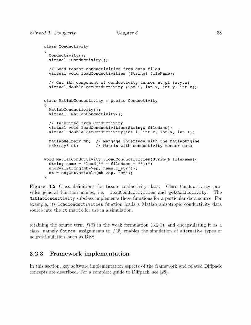
Edward T. Dougherty Chapter 3 38
class Conductivity Conductivity(); virtual ~Conductivity();
// Load tensor conductivities from data files virtual void loadConductivities (String& fileName); // Get ith component of conductivity tensor at pt (x,y,z) virtual double getConductivity (int i, int x, int y, int z);
class MatlabConductivity : public Conductivity MatlabConductivity(); virtual ~MatlabConductivity();
// Inherited from Conductivity virtual void loadConductivities(String& fileName); virtual double getConductivity(int i, int x, int y, int z);
MatlabHelper* mh; // Mangage interface with the MatlabEngine mxArray* ct; // Matrix with conductivity tensor data
void MatlabConductivity::loadConductivities(String& fileName) String name = "load('" + fileName + "');"; engEvalString(mh->ep, name.c_str()); ct = engGetVariable(mh->ep, "ct");
Figure 3.2 Class definitions for tissue conductivity data. Class Conductivity pro-vides general function names, i.e. loadConductivities and getConductivity. TheMatlabConductivity subclass implements these functions for a particular data source. Forexample, its loadConductivities function loads a Matlab anisotropic conductivity datasource into the ct matrix for use in a simulation.
retaining the source term f(~x) in the weak formulation (3.2.1), and encapsulating it as aclass, namely Source, assignments to f(~x) enables the simulation of alternative types ofneurostimulation, such as DBS.
3.2.3 Framework implementation
In this section, key software implementation aspects of the framework and related Diffpackconcepts are described. For a complete guide to Diffpack, see [28].

Edward T. Dougherty Chapter 3 39
Tissue Conductivity
Class Conductivity defines general function names, but delegates the implementation ofthese functions to its subclasses (figure 3.2). MatlabConductivity inherits Conductivity
and provides specific implementations of the loadConductivities and getConductivity
functions based on a Matlab [35] binary data file format produced by the SimNIBS softwarepackage [36].
Two additional data members are defined by MatlabConductivity, namely a MatlabHelper
object, mh, which manages a runtime interface with the MatlabEngine [35], and a Mat-lab matrix, ct. These two members are needed by the MatlabConductivity subclass,not the parent Conductivity class, and are therefore included in only the subclass. TheMatlabConductivity implementation of the loadConductivities function simply createsa Matlab command to load the anisotropic conductivity data source, executes this commandwithin the MatlabEngine via the mh object, and then stores the anisotropic conductivitytensor data into the ct matrix which are then accessible throughout a TES simulation viathe getConductivity function (figure 3.2).
The Conductivity - MatlabConductivity relationship demonstrates the advantages ofobject-oriented inheritance and polymorphism. Conductivity is used to define functionnames common to all conductivity data sources, and serves as the bridge between theserepositories and the framework. Polymorphism permits the MatlabConductivity subclassto implement specific loadConductivities and getConductivity functionality for its par-ticular data format. Code within the Conductivity class and all other framework classesdoes not dependent on these subclass implementations. Thus, alternative conductivity datasources can be easily incorporated into the framework as a subclass of Conductivity, in anidentical fashion, requiring no modification to any other framework component.
Source Term
Class Source is a software abstraction of the f(~x) source term (3.1a), and like Conductivity,defines basic functionality to be implemented in subclasses (figure 3.3). Source inherits theDiffpack class FieldFunc which allows a scalar function to be defined over the domain.Different subclass implementations of the valuePt function can be used to model differentneurostimulation modalities. For TES, valuePt in class TES_Source simply returns zerosince f(~x) = 0 in this case (figure 3.3).
Main TES Class
Class TES is the main class in the framework. Figure 3.4 presents the key elements of thisclass, which contains numerous objects, functions and Diffpack concepts. Class TES inheritsthe Diffpack FEM class, giving it access to finite element data structures and functionality.

Edward T. Dougherty Chapter 3 40
class Source: public FieldFunc TES* data; // Provides access to TES class members
Source () virtual dpreal valuePt // Source term value at pt. x; Abstract function (const Ptv(dpreal)& x, dpreal t = DUMMY) = 0;;
dpreal TES_Source:: valuePt(const Ptv(dpreal)& x, dpreal t) dpreal val = 0.0; return val;
Figure 3.3 Source term class definitions. The TES_Source subclass of Source enables TESsimulations by defining its valuePt function to return a value of zero at all points.
Handle objects, which are pointers in Diffpack that include memory management features,are defined for the computational grid, grid, and electric potential and current densitysolution results, u and currDensity respectively.
Several other class members are needed to implement TES simulations. Variables to storeboundary condition values are included, as well as the anodes and cathodes vectors to storeelectrode information. The vector isoSigma and matrix sigma store isotropic and anisotropicconductivity data, and the choice of conductivity representation is determined by a user viathe isotropic boolean variable. The mc data member is a reference to the Conductivity
class, providing an interface to conductivity data. Note that mc is type Conductivity, andnot MatlabConductivity. The mc object can therefore use the loadConductivities andgetConductivity functions of any Conductivity subclass, including MatlabConductivity.This design approach allows new Conductivity subclasses to be defined and utilized withoutthe need to modify code in class TES.
There is also a reference to a Source object, e.g. TES_Source, as well as a field func-tion for non-constant stimulation currents, e.g. tACS. Finally, TES inherits functions fromFEM to perform finite element computations, including fillEssBC to set Dirichlet boundaryconditions, calcElmMatVec to assemble the finite element linear system coefficient matrixand load vector, and the integrands and integrands4side functions to evaluate the weakformulation volume and boundary integrals, respectively.
Weak formulation integration
The weak formulation volume integrals (3.2.1) are computed in the TES integrands function(figure 3.5). The Diffpack linear system assembler automatically calls this function as ititerates over the finite elements in the computational grid. Conductivity values for thecurrent element are attained with a call to the updateConductivityTensors function, whichdetermines if isotropic or anisotropic conductivities are desired, and then populates the sigma

Edward T. Dougherty Chapter 3 41
class TES : public FEM // DATA TYPES: Handle(GridFE) grid; // Underlying finite element grid Handle(FieldFE) u; // Electric potential over grid Handle(FieldsFE) currDensity; // Electric Current density over grid
dpreal dirichlet_val1; // Constant phi value at a boundary dpreal dirichlet_val2; // Constant phi value at boundary dpreal robin_U0; // Constants for Neumann boundary condition
vector<Electrode> anodes; // Anode electrodes vector<Electrode> cathodes; // Cathode electrodes
bool isotropic; // Isotrpoic or anisotropic bool control Vec(dpreal) isoSigma; // Isotropic brain tissue conductance values MatSimple(dpreal) sigma; // Anisotropic conductivity tensor matrix Conductivity* mc; // Interface class for anisotropic conductivities
Handle(FieldFunc) source; // Source term for initializing f(x) Handle(FieldFunc) alternatingStim; // Object to model non-direct TES, i.e. tACS
// FUNCTIONS: // Standard finite element functions inherited from class FEM virtual void fillEssBC (); // Set dirichlet boundary conditions virtual void calcElmMatVec // Compute FE coefficient matrix and load vector (int e, ElmMatVec& elmat, FiniteElement& fe); virtual void integrands // Implement weak formulation integrand (ElmMatVec& elmat, const FiniteElement& fe); virtual void integrands4side // Neumann boundary integral (int side, int boind, ElmMatVec& elmat, const FiniteElement& fe);
Figure 3.4 Main elements within the TES class. Handles are Diffpack pointers that includememory management features. The class definition contains a Handle for the computa-tional grid (grid) and electric potential (u) and current density (currDensity) solutionresults. Next, variables store boundary condition values and anode (anodes) and cathode(cathodes) electrode information. Support for both isotropic and anisotropic conductiv-ity data is provided, as well as functions for source and non-constant anode stimulation.Functions inherited from FEM are required to perform finite element calculations.
matrix accordingly.
The source term f(~x) over the current element is retrieved via a call to the valuePt functionin a Source class. Then, the finite element basis functions for this element are iterated over,and the weak formulation is computed. Note that in this implementation, sigma is assumedto be diagonal, however, this can be generalized with the incorporation of an additional loop.Finally, the coefficient matrix, A, and load vector, b, are updated. The boundary integralin the weak formulation is computed similarly in the integrands4side function, and itscontribution is incorporated into b.

Edward T. Dougherty Chapter 3 42
void TES:: integrands (ElmMatVec& elmat, const FiniteElement& fe) int i,j,q; // Loop control variables const int nbf = fe.getNoBasisFunc(); // no of nodes/basis functions dpreal detJxW = fe.detJxW(); // Numerical integration weight const int nsd = fe.getNoSpaceDim(); // Number of spatial dimensions
// Get conductivity tensor for the current element. updateConductivityTensors(fe);
// Get a point in the global domain represented by elemnt fe. Ptv(NUMT) x(nsd); fe.getGlobalEvalPt(x);
// Get the source term, f(x), for this element. dpreal f_val; if (source.ok()) f_val = source->valuePt(x); else f_val = 0;
// Compute weak formulation dpreal gradNi_gradNj; for (i = 1; i <= nbf; i++) for (j = 1; j <= nbf; j++) gradNi_gradNj = 0; for (q = 1; q <= nsd; q++) // Compute inner product of grad(N_i) and grad(N_j). gradNi_gradNj += sigma(q,q) * fe.dN(i,q) * fe.dN(j,q);
// Update linear system coefficient matrix. elmat.A(i,j) += gradNi_gradNj*detJxW; // Update linear system RHS (load vector). elmat.b(i) += fe.N(i)*f_val*detJxW;
Figure 3.5 TES class integrands function for computing weak formulation volume integrals.Conductivity and source term values for finite element fe are retrieved with calls to theupdateConductivityTensors and source valuePt functions. Finite element basis functionsare then iterated to compute the volume integrals.
Multigrid
Multigrid is a linear system solution algorithm that utilizes multiple computational gridresolutions to achieve fast solution convergence [37]. By transferring the numerical residualbetween coarser and finer meshes, and performing just a few solution iterations on each, largeportions of the numerical error are efficiently removed [38]. In addition, as a preconditionerto the commonly used conjugate gradient (CG) method, MG is highly effective at solvinglinear systems that result from finite element based TES simulations [19, 39]. Two commonly

Edward T. Dougherty Chapter 3 43
used MG cycles are the V-cycle and the W-cycle, and identifying the optimal cycle type for agiven PDE system, in addition to other MG parameters including the number of grid levels,can be challenging [39].
As a subclass of TES, very few new data members and functions are needed in TES_MG
(figure 3.6), since the entirety of TES is efficiently reused. The new members in TES_MG
are a reference to the Diffpack multigrid toolbox, mgtools, and an integer representing thenumber of MG grid levels, no_of_grids. Finally, just one new function, mgFillEssBC, isneeded to set the essential boundary condition (3.1b) on all grid levels.
class TES_MG : public TES int no_of_grids; Handle(MGtools) mgtools;
// Set boundary condtion on grid level specified by space virtual void mgFillEssBC (SpaceId space);
Figure 3.6 New members of TES_MG class definition. The mgtools object references theDiffpack multigrid toolbox. The no_of_grids integer stores the number of MG grid levels,and the mgFillEssBC function sets the essential boundary condition on all grid levels.
3.2.4 Computational Tools
Numerical simulations were performed on a three-dimensional mesh (figure 3.7) generatedfrom human MRI images by the SimNIBS software package [36]. The mesh contains the skin,skull, cerebral spinal fluid (CSF), gray matter (GM), and white matter (WM) tissues of thehead. Gmsh [40] enabled mesh visualization, identification of electrode coordinates, and gridconversion to a form supported by Diffpack. Electric potential and current density resultswere exported from Diffpack and visualized with ParaView [41] and gnuplot [42]. Anisotropicconductivity data for the GM and WM regions are provided by SimNIBS in a Matlab binarydata file; these data are accessed by the MatlabEngine [35] via the MatlabHelper object ofthe MatlabConductivity class (figure 3.2).
3.2.5 Computational Simulations
Multiple simulations were performed with the TES framework. Simulations were selectedto demonstrate the framework’s versatility and ability to target medical, biophysical, andcomputational research objectives. Finally, to illustrate how alternative forms of neurostimu-lation can be simulated with the same software, we show a trivial extension to the frameworkthat enables support for DBS applications.

Edward T. Dougherty Chapter 3 44
(a) Head surface (b) Brain region (c) View of sagittal cross-section
Figure 3.7 Computational domain used in numerical simulations.
Simulation 1: Comparison of isotropic and anisotropic conductivity data
Previous research suggests that incorporating anisotropic, rather than isotropic, brain tissueconductivity data are important for most accurately modeling TES electrical current dis-tribution [17, 43]. To evaluate the impact that these two conductivity representations haveon simulation results, TES simulations were performed with isotropic and anisotropic data.The three-dimensional domain shown in figure 3.7 was used with approximately 2.8 millionlinear tetrahedra finite elements.
Anode and cathode electrodes were positioned at C3 and C4 [44], respectively, each with asurface area of approximately 16 cm2, and the anode electric current magnitude was set to 1.0mA. This montage has been used to stimulate the motor cortex ipsilateral to the C3 anodeelectrode [45, 46]. First, isotropic electrical conductivities were assigned to different tissues:skin = 0.465, skull = 0.010, CSF = 1.654, GM = 0.276, and WM = 0.126, each with units(S/m) [47]. Then, anisotropic conductivity data were used via the MatlabConductivity
class as previous described (see figure 3.2).
Simulation 2: Comparison of tDCS and HD-tDCS electrode montages
High-definition TES electrodes have demonstrated a greater ability to focus its electricalcurrent on a targeted brain region than traditional tDCS, which uses two larger electrodes[2, 3]. Using the same computational grid as Simulation 1, the current densities producedby tDCS and HD-tDCS were compared.
For tDCS, the anode was positioned over C3, and the cathode over the contralateral supra-orbital, each with a surface area of approximately 16 cm2. In comparison, high-definitionelectrodes, each circular with a 12 mm diameter, were positioned according to a 4 x 1 configu-ration; a single anode was positioned over C3, and four cathodes were placed approximately
Edward T. Dougherty Chapter 3 45
5 cm radially from the anode, forming a square. Both of these montages are known totarget the motor cortex region ipsilateral to the anode electrode [15, 48–51]. Anode stim-ulation strength for each simulation was once again 1.0 mA, and both utilized anisotropicconductivities.
Simulation 3: Comparison of finite element linear system solvers
Finite element based simulations of TES require the solution of large systems of linearequations, which can become a computational bottleneck for simulations performed on veryfine meshes. Therefore, the effectiveness of a TES simulation is directly related to theefficiency of the chosen linear solver. The CG method is ideal for solving these linear systemsand appropriate preconditioning can rapidly accelerate numerical results [37, 39].
The numerical efficiency of the preconditioned CG method was evaluated with TES simula-tions on the three-dimensional volume mesh (figure 3.7), with approximately 29 million lineartetrahedra finite elements and roughly 5.1 million unknowns. The anode was positioned atCZ, with a stimulation strength of 1.0 mA, and the cathode at OZ [12, 52]. Simulations wereperformed with the CG method preconditioned with symmetric successive over-relaxation(SSOR), relaxed incomplete LU decomposition (RILU), and multigrid. The RILU relaxationparameter was set to 0.5 [28]. The MG preconditioner was simulated with a V-cycle withboth two and three grid levels, and a W-cycle with three grid levels [19]. The relative residualconvergence tolerance was set to 10−8 for all numerical experiments.
Simulation 4: Impact of conductivity representation on DBS simulation results
The importance of incorporating anisotropic conductivities in TES simulations suggests thataccurately simulating other neurostimulation modalities may depend on this conductivityrepresentation as well. In this numerical experiment, we compared DBS simulation resultsusing both isotropic and anisotropic conductivities. A single electrode was positioned inthe subthalamatic nucleus (STN), the most commonly targeted location for DBS [53]. Theelectrode is a simplified version of the Medtronic (Model 3387) electrode used in humans [54].The lower 5.0 mm of the electrode was modeled. The anode is positioned 1.0 mm from theelectrode tip and the cathode is separated by 0.5 mm from the anode. Both the anode andcathode are 0.5 mm in height, and the overall electrode diameter was set to 0.75 mm (figure3.8). The anode and cathode metal contacts were modeled as conductors by setting theelectrical conductivities of these regions to 106 (S/m), and the remaining electrode shaft asan insulator with conductivity equal to 10−6 (S/m) [55]. Because DBS electric current isproximal to the electrode [30, 56], a 10.0 mm x 4.0 mm x 4.0 mm subset of tissue aroundthe electrode was considered as the computational domain.
To simulate DBS with the existing TES software framework, no existing code required mod-ification. Rather, the only addition was a new subclass of class Source that defines f(~x)

Edward T. Dougherty Chapter 3 46
0.75 mm
0.5 mm
0.5 mm
0.5 mm
1.0 mm
Figure 3.8 Simulation 4 DBS electrode positioning (subthalamatic nucleus) and dimensions.Anode and cathode contacts are denoted with ‘+’ and ‘–’ symbols respectively.
class DBS_Source: public Source DBS_Source(TES* data); virtual dpreal valuePt(const Ptv(dpreal)& x, dpreal t = DUMMY);;
dpreal DBS_Source:: valuePt(const Ptv(dpreal)& x, dpreal t) dpreal val = 0.0;
if (4.625 <= x(1) && x(1) <= 5.375 && 4.625 <= x(2) && x(2) <= 5.375 && 3.500 <= x(3) && x(3) <= 4.000 ) val = 0.001;
Figure 3.9 DBS_Source class definition and sample code from its valuePt function.
(3.1a) for DBS; in total, less than ten lines of code were added. Figure 3.9 displays this newsubclass definition, Source_DBS, and highlights of its valuePt function implementation,which in this simplified scenario simply injects 1.0 mA of current from the anode contactinto the surrounding tissue.

Edward T. Dougherty Chapter 3 47
3.3 Results
Simulation 1
Cu
rren
t D
en
sit
y (
A/m
2)
0.0
0.44
0.33
0.22
0.11
(a) Isotropic conductivities
Cu
rren
t D
en
sit
y (
A/m
2)
0.0
0.44
0.33
0.22
0.11
(b) Anisotropic conductivities
Figure 3.10 Simulation 1 current density results viewed from above with the nasion facingup. Anode was placed at C3 and cathode at C4.
Electric current density results on the surface of the brain tissue are displayed in figure 3.10.Viewing perspective is from above the head with the nasion facing up. As expected, thelargest electric current density values are attained near the anode and cathode locations.Despite an overall similar pattern of electric current distribution, the simulated currentdensities, particularly in the motor cortex ipsilateral to the anode electrode, are signifi-cantly different between the isotropic and anisotropic simulations. For example, the maximalanisotropic current density value (0.434 (A/m2)) is approximately 18.2% higher than in theisotropic case (0.367 (A/m2)). Similar discrepancies are observed throughout the top surfaceof the brain, including a substantial impact on the paracentral lobule contralateral to theanode. In addition, these discrepancies extend to the GM and WM interiors. These resultsreinforce the importance of using anisotropic conductivities to most accurately model TESadministrations, and in addition, showcase the capabilities of the object-oriented frameworkto support both isotropic and anisotropic TES simulations.
Simulation 2
Electric potential and electric current density results are displayed in figure 3.11. The tDCSmontage results in a noticeably larger range of electric potential values (figures 3.11a, 3.11b).

Edward T. Dougherty Chapter 3 48
Ele
ctr
ic P
ote
nti
al (V
)
0.0
0.15
0.05
0.10
(a) tDCS electric potential
Ele
ctr
ic P
ote
nti
al (V
)
0.0
0.02
0.010
0.015
0.005
(b) HD-tDCS electric potential
Cu
rre
nt
De
ns
ity
(A
/m2)
0.0
0.45
0.15
0.30
(c) tDCS electric current density
Cu
rre
nt
De
ns
ity
(A
/m2)
0.0
0.0375
0.0125
0.025
(d) HD-tDCS electric current density
Figure 3.11 Simulation 2 electric potential and current density results. The tDCS montagepositioned the anode at C3 and the cathode over the contralateral supra-orbital. A 4 x 1configuration was used for HD-tDCS with a single anode positioned over C3.
However, the focus of the tDCS current density on the targeted region, in this case the motorcortex under C3, is much less than the HD-tDCS electrode montage (figures 3.11c, 3.11d).Specifically, the brain tissue outside of the square formed by the HD-tDCS cathodes isvirtually unstimulated, whereas tDCS results in a much greater electric current dispersion.
One limitation of this HD-tDCS electrode arrangement is the lower concentration of electriccurrent that reaches the brain tissue. Specifically, the maximal electric current density in thebrain from HD-tDCS is an order of magnitude lower than tDCS. The culprit for this effectis the shunting of the electric current around the poorly conducting skull; the HD-tDCSmontage used in this simulation yields a minuscule amount of current that penetrates theskull to reach the CSF and brain tissues (figure 3.12). Potential remedies for this behaviorare a greater anode stimulation, or positioning the cathodes at greater distances from the

Edward T. Dougherty Chapter 3 49
anode [3].
This simulation demonstrates the framework’s ability to support varying TES electrodemontages, including high-definition electrode configurations. Results of this simulation cor-roborate that HD-tDCS offers greater electric current focality, however, its net stimulationof brain tissue is potentially much lower than tDCS.
Cu
rren
t D
en
sit
y (
A/m
2)
0.0
0.75
0.25
0.50
Figure 3.12 Simulation 2 HD-tDCS electric current density. Cross-section is through twodiagonally positioned cathodes.
Ele
ctr
ic P
ote
nti
al (V
)
0.0
0.12
0.04
0.08
(a) Electric potential
Cu
rren
t D
en
sit
y (
A/m
2)
0.0
2.0
0.5
1.5
1.0
(b) Current density
Figure 3.13 Simulation 3 electric potential and current density results viewed from theback of the head. The anode was positioned at CZ and the cathode at OZ.

Edward T. Dougherty Chapter 3 50
Simulation 3
Electric potential and current density results on the head surface are displayed in figure3.13. Viewing perspective is from behind the head, and as anticipated, maximal and minimalelectric potential and current density values occur at the anode and cathode, respectively.The shunting of the electric current around the skull, due to its low electrical conductivity,results in the segregated current density pattern around the anode and cathode centers (figure3.13b). This phenomena has been previously observed [1, 19], however, it is highlighted bythe very fine mesh resolution used in this simulation.
Figure 3.14 displays convergence history curves and performance metrics for each CG pre-conditioning strategy. With no preconditioning, the CG method will eventually convergence,but will accomplish this extremely slowly, requiring more than 6 hours to solve the linearsystem. The SSOR and RILU preconditioners demonstrate comparable performances, bothin solution time and number of iterations. Multigrid preconditioning with two grid levelshas far fewer iterations with 166 than both SSOR and RILU, yet has a greater run time.This observation can be explained by the fact that a single iteration of MG has embeddediterations on the different mesh refinements [38]. However, three grid level MG noticeablyaccelerates convergence rates, with both the V and W cycles outperforming the other pre-conditioners. Three grid level MG with a W-cycle pattern has slightly fewer iterations thanits corresponding V-cycle, yet this V-cycle preconditioner is approximately 11.3 % faster.
The ability of the framework to support numerically-oriented TES research is presentedin this simulation example. The results indicate that the CG method combined with anappropriately configured MG preconditioner is highly-efficient in solving the linear systemsproduced in TES computational simulations.
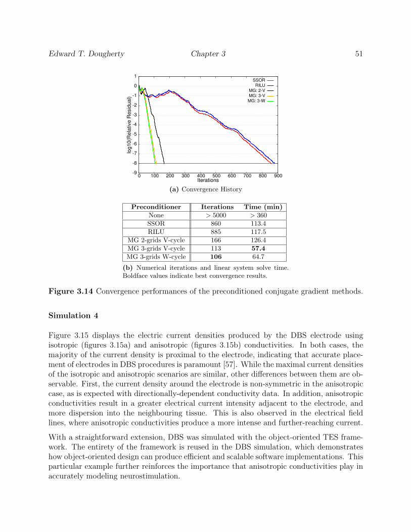
Edward T. Dougherty Chapter 3 51
-9
-8
-7
-6
-5
-4
-3
-2
-1
0
1
0 100 200 300 400 500 600 700 800 900
log10(R
ela
tive R
esid
ual)
Iterations
SSORRILU
MG: 2-VMG: 3-VMG: 3-W
(a) Convergence History
Preconditioner Iterations Time (min)None > 5000 > 360SSOR 860 113.4RILU 885 117.5
MG 2-grids V-cycle 166 126.4MG 3-grids V-cycle 113 57.4MG 3-grids W-cycle 106 64.7
(b) Numerical iterations and linear system solve time.Boldface values indicate best convergence results.
Figure 3.14 Convergence performances of the preconditioned conjugate gradient methods.
Simulation 4
Figure 3.15 displays the electric current densities produced by the DBS electrode usingisotropic (figures 3.15a) and anisotropic (figures 3.15b) conductivities. In both cases, themajority of the current density is proximal to the electrode, indicating that accurate place-ment of electrodes in DBS procedures is paramount [57]. While the maximal current densitiesof the isotropic and anisotropic scenarios are similar, other differences between them are ob-servable. First, the current density around the electrode is non-symmetric in the anisotropiccase, as is expected with directionally-dependent conductivity data. In addition, anisotropicconductivities result in a greater electrical current intensity adjacent to the electrode, andmore dispersion into the neighbouring tissue. This is also observed in the electrical fieldlines, where anisotropic conductivities produce a more intense and further-reaching current.
With a straightforward extension, DBS was simulated with the object-oriented TES frame-work. The entirety of the framework is reused in the DBS simulation, which demonstrateshow object-oriented design can produce efficient and scalable software implementations. Thisparticular example further reinforces the importance that anisotropic conductivities play inaccurately modeling neurostimulation.

Edward T. Dougherty Chapter 3 52
0.0
0.4
0.2
0.3
Cu
rre
nt
De
ns
ity
(A
/m2)
0.1
0.0
0.4
0.2
0.3
Cu
rre
nt
De
ns
ity
(A
/m2)
0.1
(a) Isotropic
0.0
0.4
0.2
0.3
Cu
rre
nt
De
ns
ity
(A
/m2)
0.1
0.0
0.4
0.2
0.3
Cu
rre
nt
De
ns
ity
(A
/m2)
0.1
(b) Anisotropic
Figure 3.15 Simulation 4 electric current density magnitudes and field lines. Currentdensities in the figures on the left are from a coronal cross-section through the electrodecenter.
3.4 Discussion
Computational simulations of neurostimulation are a valuable tool that enable researchersto investigate this form of brain therapy in silico, and as simulations become more refined,their utility to medical and biomedical research grows. While pre-built simulation softwareprograms can simplify and expedite TES model implementation, they possess applicationand portability limitations. In addition, recreating custom software as applications andresearch objectives change is inefficient, error-prone, and tedious to maintain.
Since the mathematics and physiology that governs all forms of neurostimulation is thesame, a single, well-designed software code can support a versatile range of neurostimulationsimulations. In this paper, we have presented one such software framework, described itsdesign and implementation, and demonstrated it abilities to support diverse neurostimula-

Edward T. Dougherty Chapter 3 53
tion research objectives. The cornerstone of the design stage was to encapsulate generalneurostimulation concepts into modular software objects. In doing so, a multitude of TESsimulation areas are supported, and in addition, alternative forms of neurostimulation, e.g.DBS, can be simulated with the same software.
Simulation results show the importance of using anisotropic conductivities in both TES andDBS. This is especially important for simulations utilized in selecting patient-specific neu-rostimulation parameters. In addition, results demonstrate the ability of HD-tDCS to focusthe electrical current to a specific brain region, however, this capability must be balanced witha potentially low concentration of electric current actually reaching the target. The object-oriented TES framework is an ideal tool for this scenario, enabling different permutations ofHD-tDCS electrode montages and stimulation strengths to be conveniently investigated toidentify an optimal configuration for a particular patient’s data and therapeutic objectives.
Results also illustrate that appropriately configured multigrid preconditioning can achievesuperior convergence rates. It is conceivable that hundreds of simulations could be run toidentify an optimal electrode montage and neurostimulation parameters for a particular pa-tient. Hence, efficiently solving the linear system of equations resulting from TES finiteelement simulations is crucial, and MG can be used in this capacity to greatly decreasesimulation run times. Finally, we demonstrated how a minor addition to the object-orientedTES framework enables simulations of DBS. The DBS simulation example that was per-formed is idealized, however, the simulation ensemble presented in this paper motivate howthe framework could be used to address DBS research related to electrode placement andparameter values.
In future work, we plan to extend the framework to support anisotropic transcranial magneticstimulation (TMS), in a similar fashion as was demonstrated for DBS. In addition, we planto utilize the framework to more thoroughly investigate correlations between HD-tDCS inter-electrode distances and electric current distributions.
3.5 Acknowledgements
The authors would like to acknowledge Frank Vogel and the entire inuTech team for theirassistance with Diffpack.
3.6 Bibliography
[1] A. Datta, X. Zhou, Y. Su, L. C. Parra, and M. Bikson. Validation of finite element modelof transcranial electrical stimulation using scalp potentials: implications for clinical dose.J Neural Eng, 10(3):036018, Jun 2013.

Edward T. Dougherty Chapter 3 54
[2] A. Datta, V. Bansal, J. Diaz, J. Patel, D. Reato, and M. Bikson. Gyri-precise headmodel of transcranial direct current stimulation: improved spatial focality using a ringelectrode versus conventional rectangular pad. Brain Stimul, 2(4):201–207, Oct 2009.
[3] P. Faria, M. Hallett, and P.C. Miranda. A finite element analysis of the effect of electrodearea and inter-electrode distance on the spatial distribution of the current density intDCS. J. of Neural Engineering, 8(6), 2011.
[4] P. S. Boggio, R. Ferrucci, S. P. Rigonatti, P. Covre, M. Nitsche, A. Pascual-Leone,and F. Fregni. Effects of transcranial direct current stimulation on working memory inpatients with Parkinson’s disease. J. Neurol. Sci., 249(1):31–38, Nov 2006.
[5] P. S. Boggio, L. P. Khoury, D. C. Martins, O. E. Martins, E. C. de Macedo, andF. Fregni. Temporal cortex direct current stimulation enhances performance on a vi-sual recognition memory task in Alzheimer disease. J. Neurol. Neurosurg. Psychiatr.,80(4):444–447, Apr 2009.
[6] P. S. Boggio, C. A. Valasek, C. Campanha, A. C. Giglio, N. I. Baptista, O. M. Lapenta,and F. Fregni. Non-invasive brain stimulation to assess and modulate neuroplasticityin Alzheimer’s disease. Neuropsychol Rehabil, 21(5):703–716, Oct 2011.
[7] R. Ferrucci, M. Bortolomasi, M. Vergari, L. Tadini, B. Salvoro, M. Giacopuzzi, S. Bar-bieri, and A. Priori. Transcranial direct current stimulation in severe, drug-resistantmajor depression. J Affect Disord, 118(1-3):215–219, Nov 2009.
[8] P. S. Boggio, S. P. Rigonatti, R. B. Ribeiro, M. L. Myczkowski, M. A. Nitsche,A. Pascual-Leone, and F. Fregni. A randomized, double-blind clinical trial on theefficacy of cortical direct current stimulation for the treatment of major depression. Int.J. Neuropsychopharmacol., 11(2):249–254, Mar 2008.
[9] P. Homan, J. Kindler, A. Federspiel, R. Flury, D. Hubl, M. Hauf, and T. Dierks. Mutingthe voice: a case of arterial spin labeling-monitored transcranial direct current stimu-lation treatment of auditory verbal hallucinations. Am J Psychiatry, 168(8):853–854,Aug 2011.
[10] J. Brunelin, M. Mondino, F. Haesebaert, M. Saoud, M. F. Suaud-Chagny, and E. Poulet.Efficacy and safety of bifocal tDCS as an interventional treatment for refractoryschizophrenia. Brain Stimul, 5(3):431–432, Jul 2012.
[11] A. Antal and W. Paulus. Transcranial alternating current stimulation (tACS). FrontHum Neurosci, 7:317, 2013.
[12] T. Neuling, S. Wagner, C. H. Wolters, T. Zaehle, and C. S. Herrmann. Finite-ElementModel Predicts Current Density Distribution for Clinical Applications of tDCS andtACS. Front Psychiatry, 3:83, 2012.

Edward T. Dougherty Chapter 3 55
[13] F. Gasca, L. Marshall, S. Binder, A. Schlaefer, U.G. Hofmann, and A. Schweikard. Finiteelement simulation of transcranial current stimulation in realistic rat head model. InNeural Engineering (NER), 2011 5th International IEEE/EMBS Conference on, pages36–39, April 2011.
[14] P. C. Miranda, M. Lomarev, and M. Hallett. Modeling the current distribution duringtranscranial direct current stimulation. Clin Neurophysiol, 117(7):1623–1629, Jul 2006.
[15] E. M. Caparelli-Daquer, T. J. Zimmermann, E. Mooshagian, L. C. Parra, J. K. Rice,A. Datta, M. Bikson, and E. M. Wassermann. A pilot study on effects of 41 high-definition tDCS on motor cortex excitability. Conf Proc IEEE Eng Med Biol Soc,2012:735–738, 2012.
[16] S. K. Kessler, P. Minhas, A. J. Woods, A. Rosen, C. Gorman, and M. Bikson. Dosageconsiderations for transcranial direct current stimulation in children: a computationalmodeling study. PLoS ONE, 8(9):e76112, 2013.
[17] H. S. Suh, W. H. Lee, and T. S. Kim. Influence of anisotropic conductivity in the skulland white matter on transcranial direct current stimulation via an anatomically realisticfinite element head model. Phys Med Biol, 57(21):6961–6980, Nov 2012.
[18] S. Wagner, S. M. Rampersad, U. Aydin, J. Vorwerk, T. F. Oostendorp, T. Neuling,C. S. Herrmann, D. F. Stegeman, and C. H. Wolters. Investigation of tDCS volumeconduction effects in a highly realistic head model. J Neural Eng, 11(1):016002, Feb2014.
[19] E. Dougherty, J. Turner, and F. Vogel. Efficient preconditioners and iterative methodsfor finite element based tdcs simulations. Manuscript invited for revision.
[20] S. Lew, C. H. Wolters, T. Dierkes, C. Roer, and R. S. Macleod. Accuracy and run-time comparison for different potential approaches and iterative solvers in finite elementmethod based EEG source analysis. Appl Numer Math, 59(8):1970–1988, Aug 2009.
[21] A. Wilkins. An object-oriented framework for reduced-order models using proper orthog-onal decomposition (pod). Computer Methods in Applied Mechanics and Engineering,196(4144):4375 – 4390, 2007.
[22] R. I. Mackie. An object-oriented approach to fully interactive finite element software.Adv. Eng. Softw., 29(2):139–149, March 1998.
[23] Rajiv Sampath and Nicholas Zabaras. An object-oriented framework for the implemen-tation of adjoint techniques in the design and control of complex continuum systems.International Journal for Numerical Methods in Engineering, 48(2):239–266, 2000.
[24] M. Hakman and T. Groth. Object-oriented biomedical system modeling–the rationale.Comput Methods Programs Biomed, 59(1):1–17, Apr 1999.

Edward T. Dougherty Chapter 3 56
[25] S. C. Lee, K. Bhalerao, and M. Ferrari. Object-oriented design tools for supramoleculardevices and biomedical nanotechnology. Ann. N. Y. Acad. Sci., 1013:110–123, May2004.
[26] S. Tuchschmid, M. Grassi, D. Bachofen, P. Fruh, M. Thaler, G. Szekely, and M. Harders.A flexible framework for highly-modular surgical simlation systems. In M. Harders andG. Szekely, editors, Biomedical Simulation: Third International Symposium, ISBMS2006, pages 84–92. Springer Berlin Heidelberg, 2006.
[27] A. Doronin and I. Meglinski. Online object oriented Monte Carlo computational toolfor the needs of biomedical optics. Biomed Opt Express, 2(9):2461–2469, Sep 2011.
[28] H. P. Langtangen. Computational Partial Differential Equations: Numerical Methodsand Diffpack Programming. Texts in Computational Science and Engineering. SpringerBerlin Heidelberg, 2003.
[29] H. P. Langtangen and A. Tveito. Advanced Topics in Computational Partial Differ-ential Equations: Numerical Methods and Diffpack Programming. Lecture Notes inComputational Science and Engineering. Springer Berlin Heidelberg, 2003.
[30] M. Astrom, L. U. Zrinzo, S. Tisch, E. Tripoliti, M. I. Hariz, and K. Wardell. Methodfor patient-specific finite element modeling and simulation of deep brain stimulation.Med Biol Eng Comput, 47(1):21–28, Jan 2009.
[31] Timothy Budd. An introduction to object-oriented programming. Addison-Wesley,Boston, 2002.
[32] Are Magnus Bruaset and Hans Petter Langtangen. Diffpack: A software environmentfor rapid protoptying of pde solvers.
[33] Bjarne Stroustrup. The C++ programming language. Addison-Wesley, Upper SaddleRiver, NJ, 2013.
[34] Stephen Prata. C++ primer plus. Addison-Wesley, Upper Saddle River, NJ, 2012.
[35] MATLAB. version 8.2.0.701 (R2013b). The MathWorks Inc., Natick, Massachusetts,2013.
[36] Mirko Windhoff, Alexander Opitz, and Axel Thielscher. Electric field calculations inbrain stimulation based on finite elements: An optimized processing pipeline for thegeneration and usage of accurate individual head models. Human Brain Mapping,34(4):923–935, 2013.
[37] H.A. van der Vorst. Iterative Krylov Methods for Large Linear Systems. Cambridgemonographs on applied and computational mathematics. Cambridge University Press,2003.

Edward T. Dougherty Chapter 3 57
[38] William Briggs. A multigrid tutorial. Society for Industrial and Applied Mathematics,Philadelphia, PA, 2000.
[39] K. A. Mardal, G. W. Zumbusch, and H. P. Langtangen. Software tools for multigridmethods. In H. P. Langtangen and A. Tveito, editors, Advanced Topics in Compu-tational Partial Differential Equations:Numerical Methods and Diffpack Programming,Lecture Notes in Computational Science and Engineering, pages 97–152. Springer BerlinHeidelberg, 2003.
[40] Christophe Geuzaine and Jean-Franois Remacle. Gmsh: A 3-d finite element meshgenerator with built-in pre- and post-processing facilities. International Journal forNumerical Methods in Engineering, 79(11):1309–1331, 2009.
[41] A. Henderson, J. Ahrens, and C. Law. The Paraview Guide. Kitware Inc., Clifton Park,NY, 2004.
[42] Thomas Williams, Colin Kelley, and many others. Gnuplot 4.4: an interactive plottingprogram, March 2011.
[43] A. Opitz, M. Windhoff, R. M. Heidemann, R. Turner, and A. Thielscher. How the braintissue shapes the electric field induced by transcranial magnetic stimulation. Neuroim-age, 58(3):849–859, Oct 2011.
[44] M. A. Nitsche, L. G. Cohen, E. M. Wassermann, A. Priori, N. Lang, A. Antal,W. Paulus, F. Hummel, P. S. Boggio, F. Fregni, and A. Pascual-Leone. Transcra-nial direct current stimulation: State of the art 2008. Brain Stimul, 1(3):206–223, Jul2008.
[45] M. Okamoto, H. Dan, K. Sakamoto, K. Takeo, K. Shimizu, S. Kohno, I. Oda, S. Isobe,T. Suzuki, K. Kohyama, and I. Dan. Three-dimensional probabilistic anatomical cranio-cerebral correlation via the international 10-20 system oriented for transcranial func-tional brain mapping. Neuroimage, 21(1):99–111, Jan 2004.
[46] E. K. Kang and N. J. Paik. Effect of a tDCS electrode montage on implicit motorsequence learning in healthy subjects. Exp Transl Stroke Med, 3(1):4, 2011.
[47] A. Datta, J. M. Baker, M. Bikson, and J. Fridriksson. Individualized model predictsbrain current flow during transcranial direct-current stimulation treatment in responsivestroke patient. Brain Stimul, 4(3):169–174, Jul 2011.
[48] G. Schlaug, V. Renga, and D. Nair. Transcranial direct current stimulation in strokerecovery. Arch. Neurol., 65(12):1571–1576, Dec 2008.
[49] A. F. DaSilva, M. S. Volz, M. Bikson, and F. Fregni. Electrode positioning and montagein transcranial direct current stimulation. J Vis Exp, (51), 2011.

Edward T. Dougherty Chapter 3 58
[50] A. Antal, D. Terney, C. Poreisz, and W. Paulus. Towards unravelling task-related mod-ulations of neuroplastic changes induced in the human motor cortex. Eur. J. Neurosci.,26(9):2687–2691, Nov 2007.
[51] D. Q. Truong, G. Magerowski, G. L. Blackburn, M. Bikson, and M. Alonso-Alonso.Computational modeling of transcranial direct current stimulation (tDCS) in obesity:Impact of head fat and dose guidelines. Neuroimage Clin, 2:759–766, 2013.
[52] A. Antal, K. Boros, C. Poreisz, L. Chaieb, D. Terney, and W. Paulus. Comparativelyweak after-effects of transcranial alternating current stimulation (tACS) on corticalexcitability in humans. Brain Stimul, 1(2):97–105, Apr 2008.
[53] S. Miocinovic, S. Somayajula, S. Chitnis, and J. L. Vitek. History, applications, andmechanisms of deep brain stimulation. JAMA Neurol, 70(2):163–171, Feb 2013.
[54] L. M. Zitella, K. Mohsenian, M. Pahwa, C. Gloeckner, and M. D. Johnson. Compu-tational modeling of pedunculopontine nucleus deep brain stimulation. J Neural Eng,10(4):045005, Aug 2013.
[55] S. Miocinovic, M. Parent, C. R. Butson, P. J. Hahn, G. S. Russo, J. L. Vitek, andC. C. McIntyre. Computational analysis of subthalamic nucleus and lenticular fasciculusactivation during therapeutic deep brain stimulation. J. Neurophysiol., 96(3):1569–1580,Sep 2006.
[56] C. C. McIntyre and T. J. Foutz. Computational modeling of deep brain stimulation.Handb Clin Neurol, 116:55–61, 2013.
[57] Daniel Tarsy. Deep brain stimulation in neurological and psychiatric disorders. HumanaPress, Totowa, NJ, 2008.

Chapter 4
Multiscale Coupling of TranscranialDirect Current Stimulation to NeuronElectrodynamics: Modeling theInfluence of the Transcranial ElectricField on Neuronal Depolarization
Edward Dougherty, James Turner, and Frank Vogel
Edward T. Dougherty, James C. Turner, and Frank Vogel, “Multiscale Coupling of Transcra-nial Direct Current Stimulation to Neuron Electrodynamics: Modeling the Influence of theTranscranial Electric Field on Neuronal Depolarization,” Computational and MathematicalMethods in Medicine, vol. 2014, Article ID 360179, 14 pages, 2014
59

Edward T. Dougherty Chapter 4 60
Abstract
Transcranial direct current stimulation (tDCS) continues to demonstrate success as a medicalintervention for neurodegenerative diseases, psychological conditions, and traumatic braininjury recovery. One aspect of tDCS still not fully comprehended is the influence of thetDCS electric field on neural functionality. To address this issue, we present a mathematical,multiscale model that couples tDCS administration to neuron electrodynamics. We demon-strate the model’s validity and medical applicability with computational simulations usingan idealized two-dimensional domain, and then an MRI-derived, three-dimensional humanhead geometry possessing inhomogeneous and anisotropic tissue conductivities. We exem-plify the capabilities of these simulations with real-world tDCS electrode configurations andtreatment parameters, and compare the model’s predictions to those attained from medicalresearch studies. The model is implemented using efficient numerical strategies and solutiontechniques to allow the use of fine computational grids needed by the medical community.

Edward T. Dougherty Chapter 4 61
4.1 Introduction
Transcranial direct current stimulation (tDCS) is a medical procedure that delivers electricalstimulation to the brain through electrodes positioned on the scalp. The electrodes deliver anelectrical current on the order of 1-2 mA, and produce an electric field in the patient’s cerebralcavity that alters neuron excitability. A common use of this treatment is to assist neuronsin firing action potentials (APs) by increasing their resting membrane potential. Currentbiomedical research continues to demonstrate the benefits of tDCS as a medical treatment.Recognition memory in Alzheimer disease patients has improved [1, 2]. Individuals whosuffer from Parkinson’s disease have demonstrated enhanced physical and mental skills [3, 4].Patients diagnosed with neuropsychiatric disorders, including great depression, have shownimproved cognitive capabilities [5, 6]. Further, post-stroke recovery can be expedited withstrategic administrations of tDCS [7, 8].
Current components of tDCS include the Laplace equation [9–13], which is given by
∇ ·M∇Φ = 0, ~x ∈ Ω (4.1)
where Φ is the electric potential, M represents the tissue conductivity tensor field, and Ω isthe entire head cavity, including the brain. In isotropic tissues, M can be represented as ascalar which will vary among different tissue types.
Computational simulations of tDCS that utilize (4.1) have the capability to compute thestrength of the tDCS electric potential and electric current at specific points in the brainand head cavity [11, 14]. What these models do not have, however, is the capability toprovide a description of cellular-level functionality. The fundamental objective of tDCS is toalter neuron excitability by increasing or decreasing neural transmembrane voltage [15, 16];without this level of biological abstraction included in a tDCS model, it is not possible toexamine tDCS effects on brain cells within a computational simulation.
Beyond the tDCS modeling and simulation field, the computational neuroscience commu-nity possesses a large collection of biologically-inspired, mathematical models of neural-leveldynamics. The Hodgkin-Huxley model, for example, emulates voltage-gated ion channelfunctionality [17]. The Hindmarsh-Rose model incorporates neuron bursting, which is thediverse and chaotic behavior of rapid action potential spiking, believed to be very importantin information encoding and propagation [18]. More recently, models have included indi-vidual neurotransmitter species, receptors, and binding kinetics to emulate neuron-neuroninfluences and communication [19].
A multi-scale model that couples tDCS and cellular level functionality would enable re-searchers to simulate the impact that tDCS has on neurons. For instance, correlations be-tween tDCS and ion channel functionality, action potential behavior, and neurotransmitterdynamics could be studied. In addition, patient-specific electrode configurations and treat-ment parameters could be optimized based on neuron behavior. Furthermore, a multi-scalemodel would provide a bridge between the tDCS numerical simulation field and the compu-

Edward T. Dougherty Chapter 4 62
tational neuroscience field, thereby enabling tDCS simulations access to the sophisticated,physiologically-based cellular and sub-cellular models of the neuroscience community.
Several researchers have investigated the influence of extra-cellular electrical fields on thetransmembrane voltage of individual and small groups of cells [15, 16, 20, 21]. At the organlevel, Szmurlo et al. [22, 23] demonstrated the applicability of the bidomain model [24] (seeSec. 4.2.1) to electroencephalograph (EEG) applications. They showed that this model,which has historically been used in cardiac applications, can reproduce scalp surface electricpotential measurements originating from neuron action potentials.
In this paper, we combine these modeling strategies to produce a multi-scale model of tDCS.We begin by coupling the bidomain model partial differential equations (PDEs) with bound-ary conditions that model tDCS treatments. We validate the model against several test caseson two different geometries. First, we simulate the model on an idealized two-dimensionaldomain, which provides a basic environment for visualizing and investigating electric poten-tial and electric field characteristics. Then, we utilize an MRI-derived, three-dimensionalhuman head geometry that possesses inhomogeneous and anisotropic tissue conductivities.In this setting, we examine the electric potential, electric current, electric field, and trans-membrane voltage results produced from real-world tDCS electrode configurations. In bothgeometries, five distinct tissue types are used: skin, skull, cerebrospinal fluid (CSF), andthe grey matter (GM) and white matter (WM) portions of the brain. Further, we detailthe numerical methods and solution techniques that we implemented to enable reasonablesimulation execution times.
To our knowledge, this paper presents the first multiscale tDCS model and simulations.We hope that the modeling and computational approaches presented in this paper help toexpand tDCS simulation capabilities, and further our understanding of tDCS impacts at thecellular level.
4.2 Materials and Methods
This section presents details of the model, numerics, and computational simulations used inthis paper. First, an overview of the bidomain model is provided, as well as a descriptionof the adaptation of this model for tDCS. Then, the numerical methods used to implementthe multiscale tDCS model are described. Next, an overview of computational tools that weutilized is presented. Finally, the numerical experiments that were performed are described.
4.2.1 Bidomain Model
Modeling each cell in the brain and head is not computationally feasible; the bidomain modelis based on a volume averaging approach, where the value at a point in a tissue is treated

Edward T. Dougherty Chapter 4 63
as an average over a minuscule, multi-cellular region around the point [25]. The bidomainmodel, as its name implies, models two domains, namely the intracellular and extracellularspaces. Each of these domains is considered continuous within the brain, and they areinsulated from each by the cell membrane. Transcellular electric current is possible via ionchannels in the cell membrane, and the transmembrane electric potential is defined to be thedifference between intracellular and extracellular electric potentials, v = Φi − Φe.
The bidomain model is given by the following system of partial differential equations forpoints in the brain, ~x ∈ ΩB:
∇ · (Mi∇v) +∇ · (Mi∇Φe) = χCm∂v
∂t+ χIion, (4.2)
∇ · (Mi∇v) +∇ · ((Mi + Me)∇Φe) = 0, (4.3)
∂~s
∂t= F (~s, v, t), (4.4)
where Φe = Φe(~x, t) is the extracellular electric potential and v = v(~x, t) is the transmem-brane voltage. Note that in this formulation, Φi has been eliminated with the substitutionof v; if desired, Φi can be computed at any point in the domain using Φi = v + Φe. Mi
and Me represent the intracellular and extracellular tissue conductivity tensor fields, re-spectively. In addition, χ is the cell membrane surface to volume ratio and Cm is the cellmembrane capacitance. Iion = Iion(~s, v, t) is the total ionic current between the intracellularand extracellular domains, across the cell membrane. Equation 4.4, which characterizes theelectrophysiological state of the neurons, can be represented by a single equation or by asystem of ordinary differential equations (ODEs) [25].
Equations (4.2-4.4) are defined in the brain. Outside of the brain tissue, the scalp, skull, andcerebrospinal fluid are modeled as a passive conductor with the Laplace equation (4.1). Inthis extra-cerebral domain, neurons and other electrically responsive cells are not present,and so only the extracellular domain exists. Thus, the intracellular current is confined to thebrain; this condition is enforced by requiring that the outflow of intracellular current fromthe brain into the extra-cerebral region equals zero:
~n · (Mi∇(v + Φe)) = 0, ~x ∈ ∂ΩB,
where ∂ΩB is the surface boundary of the brain.
Extracellular electric field continuity at the interface between the brain and extra-cerebraldomain is preserved by requiring that ~n · (Me∇Φe) and Φe are continuous over ∂ΩB. Tosimplify notation, for the remainder of this paper Φe will be represented simply as Φ.
4.2.2 tDCS Adaptation
To make the bidomain model suitable for tDCS applications, two specific areas need to beaddressed. First, the boundary conditions on the scalp must model tDCS administration.
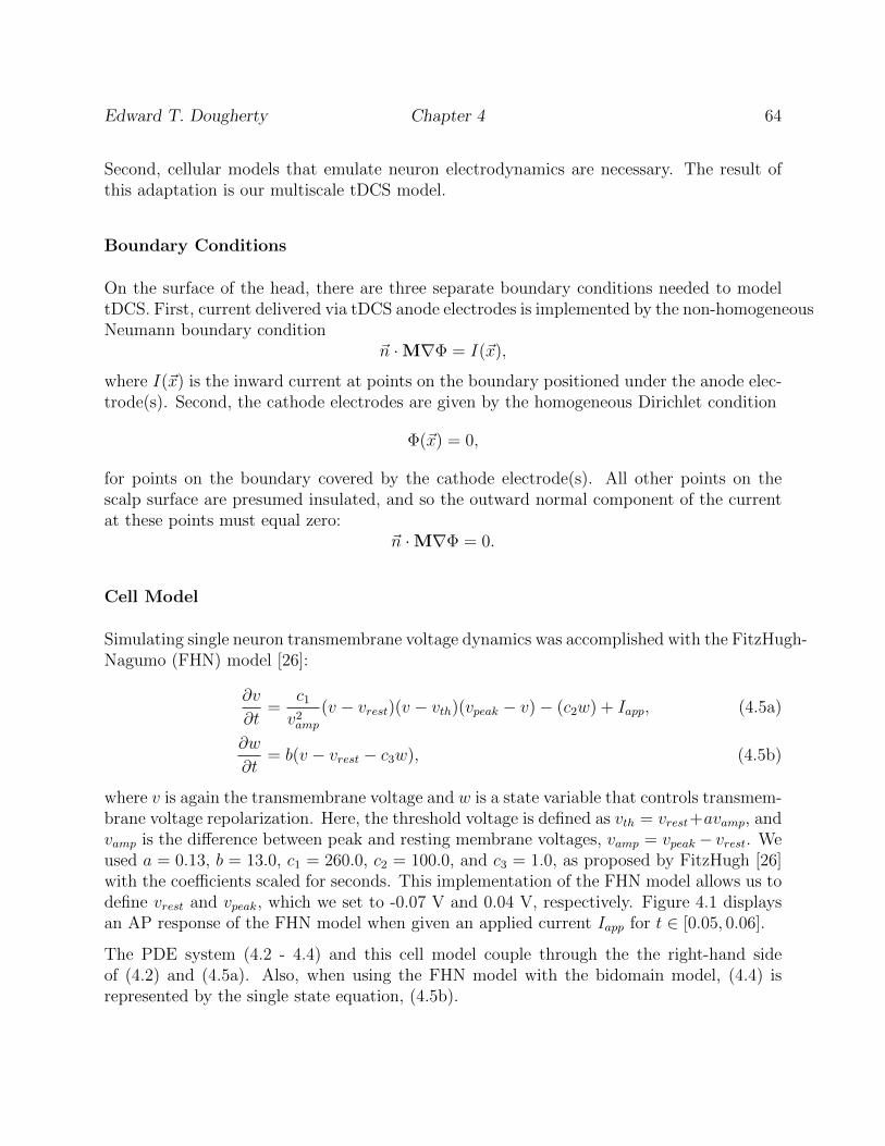
Edward T. Dougherty Chapter 4 64
Second, cellular models that emulate neuron electrodynamics are necessary. The result ofthis adaptation is our multiscale tDCS model.
Boundary Conditions
On the surface of the head, there are three separate boundary conditions needed to modeltDCS. First, current delivered via tDCS anode electrodes is implemented by the non-homogeneousNeumann boundary condition
~n ·M∇Φ = I(~x),
where I(~x) is the inward current at points on the boundary positioned under the anode elec-trode(s). Second, the cathode electrodes are given by the homogeneous Dirichlet condition
Φ(~x) = 0,
for points on the boundary covered by the cathode electrode(s). All other points on thescalp surface are presumed insulated, and so the outward normal component of the currentat these points must equal zero:
~n ·M∇Φ = 0.
Cell Model
Simulating single neuron transmembrane voltage dynamics was accomplished with the FitzHugh-Nagumo (FHN) model [26]:
∂v
∂t=
c1
v2amp
(v − vrest)(v − vth)(vpeak − v)− (c2w) + Iapp, (4.5a)
∂w
∂t= b(v − vrest − c3w), (4.5b)
where v is again the transmembrane voltage and w is a state variable that controls transmem-brane voltage repolarization. Here, the threshold voltage is defined as vth = vrest+avamp, andvamp is the difference between peak and resting membrane voltages, vamp = vpeak− vrest. Weused a = 0.13, b = 13.0, c1 = 260.0, c2 = 100.0, and c3 = 1.0, as proposed by FitzHugh [26]with the coefficients scaled for seconds. This implementation of the FHN model allows us todefine vrest and vpeak, which we set to -0.07 V and 0.04 V, respectively. Figure 4.1 displaysan AP response of the FHN model when given an applied current Iapp for t ∈ [0.05, 0.06].
The PDE system (4.2 - 4.4) and this cell model couple through the the right-hand sideof (4.2) and (4.5a). Also, when using the FHN model with the bidomain model, (4.4) isrepresented by the single state equation, (4.5b).
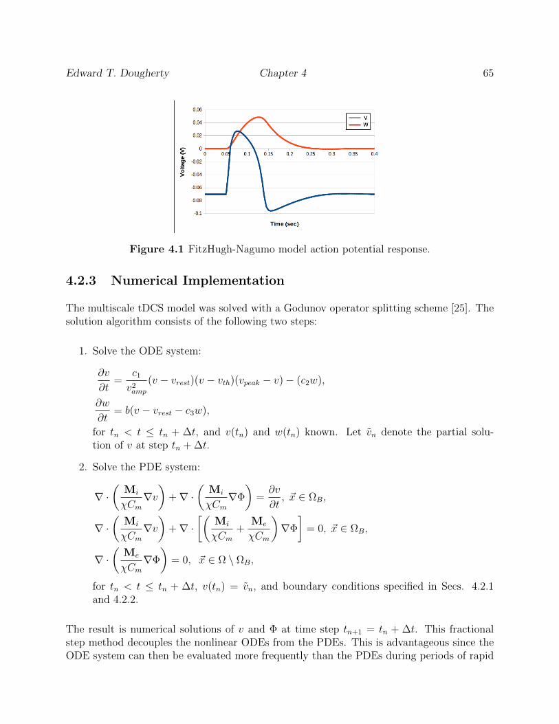
Edward T. Dougherty Chapter 4 65
Figure 4.1 FitzHugh-Nagumo model action potential response.
4.2.3 Numerical Implementation
The multiscale tDCS model was solved with a Godunov operator splitting scheme [25]. Thesolution algorithm consists of the following two steps:
1. Solve the ODE system:
∂v
∂t=
c1
v2amp
(v − vrest)(v − vth)(vpeak − v)− (c2w),
∂w
∂t= b(v − vrest − c3w),
for tn < t ≤ tn + ∆t, and v(tn) and w(tn) known. Let vn denote the partial solu-tion of v at step tn + ∆t.
2. Solve the PDE system:
∇ ·(
Mi
χCm∇v)
+∇ ·(
Mi
χCm∇Φ
)=∂v
∂t, ~x ∈ ΩB,
∇ ·(
Mi
χCm∇v)
+∇ ·[(
Mi
χCm+
Me
χCm
)∇Φ
]= 0, ~x ∈ ΩB,
∇ ·(
Me
χCm∇Φ
)= 0, ~x ∈ Ω \ ΩB,
for tn < t ≤ tn + ∆t, v(tn) = vn, and boundary conditions specified in Secs. 4.2.1and 4.2.2.
The result is numerical solutions of v and Φ at time step tn+1 = tn + ∆t. This fractionalstep method decouples the nonlinear ODEs from the PDEs. This is advantageous since theODE system can then be evaluated more frequently than the PDEs during periods of rapid

Edward T. Dougherty Chapter 4 66
transmembrane voltage change, i.e. AP spiking, without having to also solve the computa-tionally intensive PDE system. In addition, this Godunov splitting scheme is numericallystable and computationally efficient [27].
The ODE system in step 1 is solved with Heun’s method [28]. The PDE system in step 2is solved as a coupled system, discretizing in time with the implicit Euler method, and inspace with the finite element method [29]. The resulting finite element formulation yieldsthe following system of equations in block matrix form [25]:(
A BBT C
)(~v~Φ
)=
(~α~0
), (4.6)
where the ith and jth entries are given by:
Aij =
∫ΩB
NjNi dx+∆t
χCm
∫ΩB
Mi∇Nj · ∇Ni dx,
Bij =∆t
χCm
∫ΩB
Mi∇Nj · ∇Ni dx,
Cij =∆t
χCm
∫ΩB
(Mi + Me)∇Nj · ∇Ni dx +
∆t
χCm
∫Ω\ΩB
Me∇Nj · ∇Ni dx,
αi =
∫ΩB
vnNi dx,
and vj and Φj are the unknown transmembrane and electric potentials that together form thesolution that we seek. Here, Ni and Nj are finite element basis functions over the discretizeddomain.
The linear system (4.6) is solved by the conjugate gradient method [30] preconditioned withthe following block preconditioner [29]:
K =
(A−1 0
0 C−1
), (4.7)
where A−1 and C−1 are incomplete LU (ILU) factorizations [31] of A and C, respectively.
4.2.4 Computational Tools
Several of the multiscale tDCS numerical simulations are performed on a three-dimensionalgrid derived from human MRI data. The SimNIBS software package [32] provides the as-

Edward T. Dougherty Chapter 4 67
sociated computational grid; it is a high-quality tetrahedral mesh of the scalp, skull, CSF,GM and WM. Gmsh [33] supported mesh visualization, and supplied grid file conversion toa format supported by Diffpack 1 [34]. Figure 4.2 displays portions of the computationalmesh used in the three-dimensional simulations.
(a) Head boundary of mesh (b) WM and GM portion of mesh
Figure 4.2 Portions of the computational grid used in multiscale tDCS simulations.
Finite element solutions were performed with Diffpack. An anisotropic conductivity tensorfield for the brain region of the MRI-derived mesh is generated by SimNIBS and stored in aMatlab [35] binary data file; the Matlab engine was invoked and utilized in our C++ codeto access these tensor data at run-time. The ODE solver (Heun’s method) was implementedin C++, and the operator splitting scheme was performed with Diffpack. In addition, theblock coefficient matrix (4.6) and block preconditioner (4.7) were implemented with Diffpack.Results were exported to VTK format and visualized with ParaView2.
4.2.5 Multiscale tDCS Numerical Experiments
Numerical experiments were contrived to examine the following four properties:
1. Action potential conduction velocity;
2. tDCS electric potential;
3. tDCS electric current and field; and
4. tDCS-induced transmembrane voltage increase.
1www.diffpack.com/2www.paraview.org/
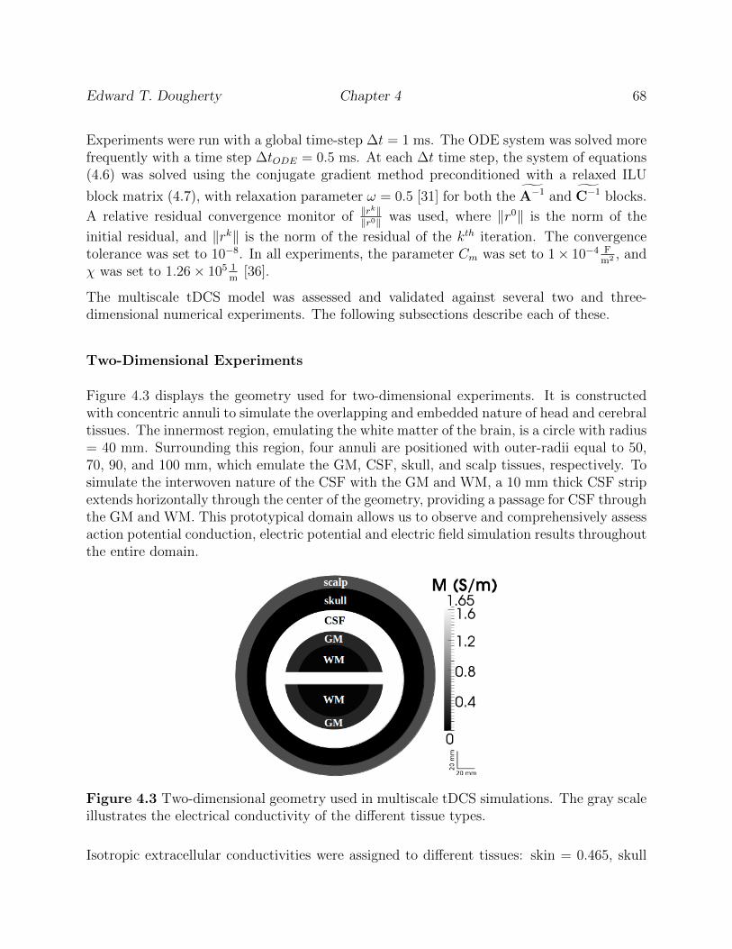
Edward T. Dougherty Chapter 4 68
Experiments were run with a global time-step ∆t = 1 ms. The ODE system was solved morefrequently with a time step ∆tODE = 0.5 ms. At each ∆t time step, the system of equations(4.6) was solved using the conjugate gradient method preconditioned with a relaxed ILU
block matrix (4.7), with relaxation parameter ω = 0.5 [31] for both the A−1 and C−1 blocks.
A relative residual convergence monitor of ‖rk‖‖r0‖ was used, where ‖r0‖ is the norm of the
initial residual, and ‖rk‖ is the norm of the residual of the kth iteration. The convergencetolerance was set to 10−8. In all experiments, the parameter Cm was set to 1× 10⁻⁴ F
m2 , andχ was set to 1.26× 10⁵ 1
m[36].
The multiscale tDCS model was assessed and validated against several two and three-dimensional numerical experiments. The following subsections describe each of these.
Two-Dimensional Experiments
Figure 4.3 displays the geometry used for two-dimensional experiments. It is constructedwith concentric annuli to simulate the overlapping and embedded nature of head and cerebraltissues. The innermost region, emulating the white matter of the brain, is a circle with radius= 40 mm. Surrounding this region, four annuli are positioned with outer-radii equal to 50,70, 90, and 100 mm, which emulate the GM, CSF, skull, and scalp tissues, respectively. Tosimulate the interwoven nature of the CSF with the GM and WM, a 10 mm thick CSF stripextends horizontally through the center of the geometry, providing a passage for CSF throughthe GM and WM. This prototypical domain allows us to observe and comprehensively assessaction potential conduction, electric potential and electric field simulation results throughoutthe entire domain.
Figure 4.3 Two-dimensional geometry used in multiscale tDCS simulations. The gray scaleillustrates the electrical conductivity of the different tissue types.
Isotropic extracellular conductivities were assigned to different tissues: skin = 0.465, skull

Edward T. Dougherty Chapter 4 69
= 0.010, CSF = 1.654, GM = 0.276, and WM = 0.126, each with units Sm
[37], and anintracellular conductivity value of 0.1 S
mwas used in the GM and WM. Each experiment
included 10,000 linear triangular finite elements.
Individual two-dimensional experiments are described in the following paragraphs:
Action potential conduction:An AP centered at (0, -25), encompassing a circular region with radius = 2.5 mm,was simulated for t ∈ (0, 10] ms. Total simulation time is 100 ms. tDCS was notadministered and so the homogeneous Neumann boundary condition ~n·Me∇Φ = 0 wasimposed on the entire scalp surface. This experiment is used to ensure the biologicallegitimacy of the multiscale model’s AP conduction velocity, and in doing so verifiesthat appropriate parameter values were selected. This experiment is also used toexamine the electric potential, Φ, produced by the AP.
tDCS electric potential and field:Models of tDCS based on the Laplace equation (4.1) accurately quantify tDCS electricpotentials and fields [11, 14]. Therefore, to validate the multiscale model, its elec-tric potential and electric field simulation results are compared to those produced byequation (4.1).
These comparisons are performed using two simulations. First, tDCS was simulatedwith the anode and cathode electrodes positioned at (-100, 0) and (70.7, 70.7) respec-tively. Electrode size is 10 mm, and the anode electric current magnitude was set to1.0 mA (see Sec. 4.2.2) at t = 0. No AP was artificially initiated, i.e. Iapp = 0 (4.5a),and simulation duration is 100 ms.
This numerical experiment was repeated with a different electrode configuration, plac-ing the anode electrode at (-70.7, 70.7) and the cathode at (0, -100). This electrodearrangement was selected to provide substantive differences from the first arrangement.First, the electric current entry via the anode does not neighbor the central CSF chan-nel, as is the case with the first electrode configuration. Second, the current exit atthe cathode electrode is as distant from the central CSF channel as possible in thistwo-dimensional domain. In addition, the anode and cathode are on opposite sides ofthe CSF channel in the second configuration.
Three-Dimensional Experiments
Three-dimensional experiments were conducted on an MRI-derived volume mesh. Figure4.2 displays portions of the mesh used in these simulations. Extracellular conductivitiesof the scalp, skull, and CSF were isotropic, and set to 0.465 S
m, 0.010 S
m, and 1.654 S
m,
respectively [37]. Anisotropic extracellular conductivities of the GM and WM portions ofthe brain were used; this tensor field is provided by the SimNIBS software package (see Sec.4.2.4). The intracellular conductivity for the brain region was set to 0.1 S
m.

Edward T. Dougherty Chapter 4 70
Table 4.1 Multiscale tDCS three-dimensional numerical experiment electrode configura-tions. Specified using the international 10-20 system.
Anode Cathode(s) Target Region
Montage 1 C3 C4 Motor cortex (ipsilateral to anode)
Montage 2 C3 Fp2 Motor cortex (ipsilateral to anode)
Montage 3 Forehead symmetric Mastoids (both) Motor cortex; STN and SN
Three separate electrode montages were selected for the three-dimensional simulations (seeTable 4.1). Each montage is specified using the international 10-20 system [38]. Transcra-nial direct current stimulation applied with montage 1 has shown to enhance motor sequencelearning [39], for example. This montage is known to target the motor cortex region ipsilat-eral to the anode electrode [40]. Montage 2 has been utilized in a host of biomedical researchstudies involving motor-skills and also enhances neural tissue excitability in the motor cortexipsilateral to the anode [38]. Montage 3 has been shown to improve gait and bradykinesia inpatients with Parkinson’s disease [3]. It remains unclear, however, the regions of the brainand the mechanisms by which tDCS enhances motor performance in these individuals. Neu-rostimulation research suggests that stimulation of the primary motor cortex is a catalystfor motor-skill improvement [3, 41]. In addition, other research studies verify that electricalstimulation to the subthalamic nucleus (STN) and substantia nigra (SN) greatly improvesmotor performance in Parkinson’s disease patients [42–46].
In all montages, the anode electric current magnitude was set to 1.0 mA (see Sec. 4.2.2)at t = 0 and the surface area of each electrode is approximately 25 cm2 [3, 39]. Numericalexperiments were run for 100 ms, and no APs were forced, i.e. Iapp = 0 (4.5a). The headgeometry is comprised of approximately 1.1 million linear tetrahedra finite elements.
Again, the Laplace equation (4.1) accurately models tDCS electric potentials and fields[11, 14]. For each montage, the multiscale model is validated by comparing its scalp sur-face electric potential simulation results against those generated by Laplace equation-basedsimulations. A similar comparison is performed with the tDCS electric current and field.Then, the multiscale model’s ability to predict the areas of the brain that become moreexcitable from tDCS treatments administered with these three montages is verified. Thisis accomplished by examining the transmembrane voltage increase in those regions of thebrain known to become more excitable from tDCS. For montages 1 and 2, the motor cortexipsilateral to the anode is examine, and for montage 3 the motor cortex and the STN andSN regions are inspected (see Table 4.1).

Edward T. Dougherty Chapter 4 71
4.3 Results and Discussion
4.3.1 Two-dimensional simulations
Action potential conduction
Transmembrane voltage results for the AP numerical experiment described in Sec 4.2.5 arepresented in Fig. 4.4. Figure 4.4a shows the start of the AP. By time t = 10 ms, APdispersion is quite noticeable (Fig. 4.4b). The conduction velocity is approximately 2.0 m
s.
This value is on the lower end of normal neural conduction velocities [47], however, averageAP speed varies among individuals and testing conditions [48]. In addition, the conductionvelocity can easily be adjusted in the model by changing χ, Cm, Mi, or Me. Further,alternative neuron models possess different AP transmembrane voltage upstroke rates thatwill affect conduction velocity [25].
(a) Transmembrane voltage at time t=1 ms (b) Transmembrane voltage at time t=10 ms
Figure 4.4 Action potential conduction in two-dimensional geometry.
Figure 4.5 displays the electric potential, Φ, produced from the AP. Figure 4.5a shows Φthroughout the entire two-dimensional domain at t = 46 ms. Variability in the electricpotential due to the inhomogeneous extracellular conductivities is noticeable. Figure 4.5bdisplays electric potential time-course plots, for points at the center of the domain andsurface boundary that intersect each Cartesian axis. The curves representing the points thatintersect the x-axis, namely (-100, 0) and (100, 0), are similar due to their symmetry withrespect to the AP. However, all other curves show variability due to their spacial separationand tissue conductivity inhomogeneity.
These electric potential results are of the same order of magnitude as those reported bySzmurlo et al. [22]. Further, they are several orders of magnitude lower than those producedduring tDCS sessions [37]. These results are consistent with the observation that head surface

Edward T. Dougherty Chapter 4 72
(a) Electric potential at time t = 46 ms (b) Electric potential time-course plots at five points in thedomain
Figure 4.5 Electric potential (Φ) from action potential.
electric potential measurements are dominated by the tDCS electric current with negligibleimpact from AP conduction [49].
This numerical experiment confirms that the selected parameter set produces biologicallyreasonable action potential results. Conduction speeds are appropriate and the electricpotential resulting from an AP is consistent with previous research reports. In the followingsections, the multiscale model is validated when tDCS is administered.
tDCS administration
First electrode configuration:
Electric potential simulation results for the Laplace equation-based model and the multiscalemodel are presented in Fig. (4.6). The electric potential of the Laplace model (Fig. 4.6a)closely resembles the multiscale model’s electric potential at both t = 1 ms (Fig. 4.6b)and t = 25 ms (Fig. 4.6c). The electric potential difference between these two times hasminuscule change. For t > 25 ms, the electric potential stabilizes, and no visible differenceswere observed throughout the remainder of the simulation.
Figure 4.7 displays the tDCS electric fields for the Laplace and multiscale models. Multiscalemodel results are shown at t = 1 ms, but they are essentially identical at all times. Differ-ences between the models’ electric current densities and fields are virtually indistinguishable.The tendency of the electric field to shunt the skull is due to the low conductivity of thistissue, and this produces an increased current density exiting the edges of the anode andentering the edges of the cathode [11]. In addition, the portion of the electric current thatpenetrates the skull has high affinity for the highly conductive CSF.
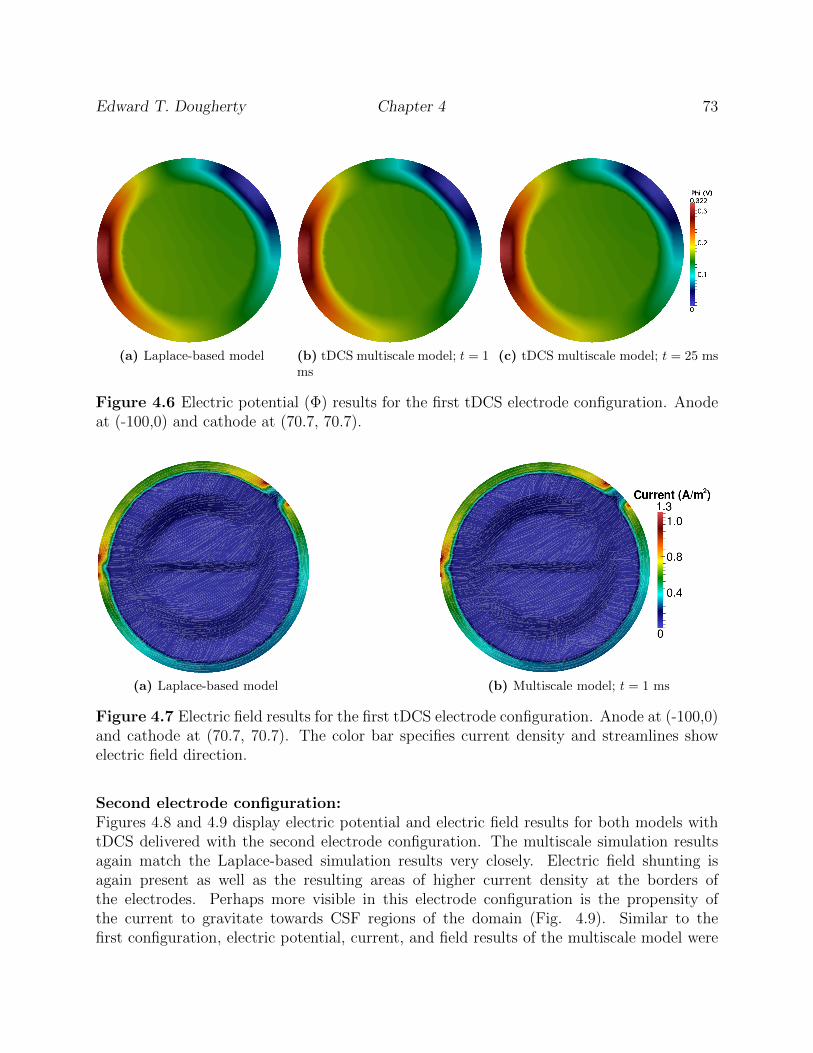
Edward T. Dougherty Chapter 4 73
(a) Laplace-based model (b) tDCS multiscale model; t = 1ms
(c) tDCS multiscale model; t = 25 ms
Figure 4.6 Electric potential (Φ) results for the first tDCS electrode configuration. Anodeat (-100,0) and cathode at (70.7, 70.7).
(a) Laplace-based model (b) Multiscale model; t = 1 ms
Figure 4.7 Electric field results for the first tDCS electrode configuration. Anode at (-100,0)and cathode at (70.7, 70.7). The color bar specifies current density and streamlines showelectric field direction.
Second electrode configuration:Figures 4.8 and 4.9 display electric potential and electric field results for both models withtDCS delivered with the second electrode configuration. The multiscale simulation resultsagain match the Laplace-based simulation results very closely. Electric field shunting isagain present as well as the resulting areas of higher current density at the borders ofthe electrodes. Perhaps more visible in this electrode configuration is the propensity ofthe current to gravitate towards CSF regions of the domain (Fig. 4.9). Similar to thefirst configuration, electric potential, current, and field results of the multiscale model were
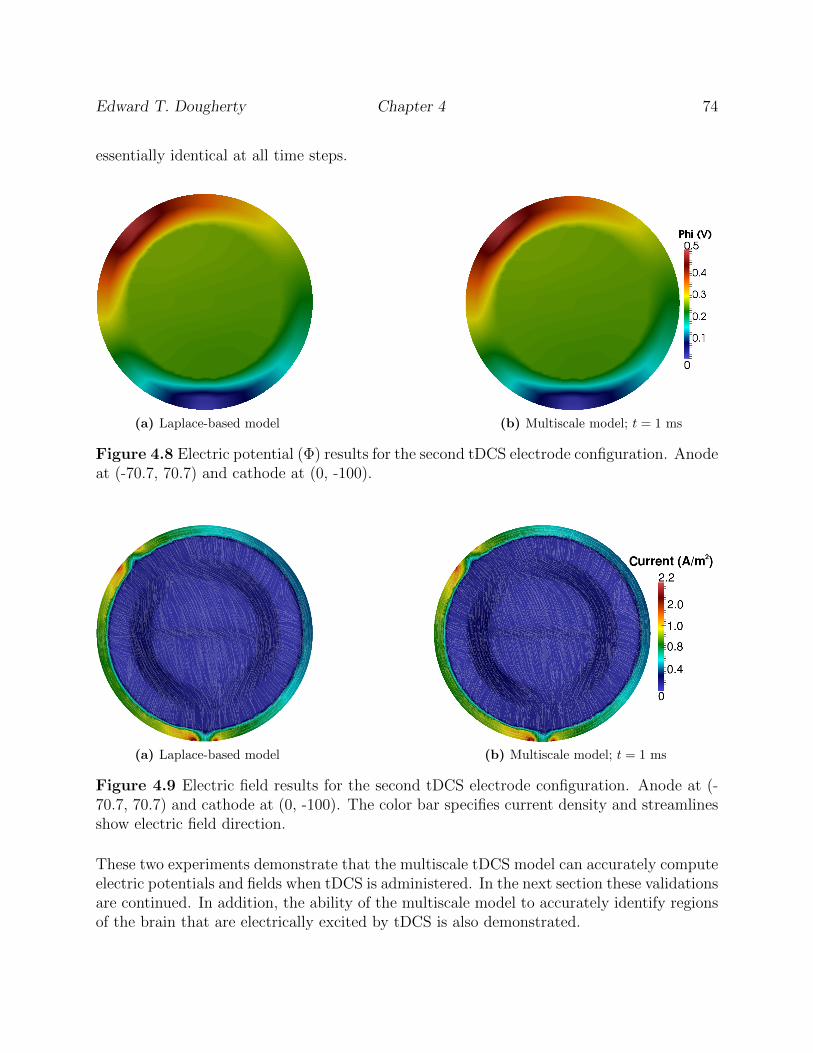
Edward T. Dougherty Chapter 4 74
essentially identical at all time steps.
(a) Laplace-based model (b) Multiscale model; t = 1 ms
Figure 4.8 Electric potential (Φ) results for the second tDCS electrode configuration. Anodeat (-70.7, 70.7) and cathode at (0, -100).
(a) Laplace-based model (b) Multiscale model; t = 1 ms
Figure 4.9 Electric field results for the second tDCS electrode configuration. Anode at (-70.7, 70.7) and cathode at (0, -100). The color bar specifies current density and streamlinesshow electric field direction.
These two experiments demonstrate that the multiscale tDCS model can accurately computeelectric potentials and fields when tDCS is administered. In the next section these validationsare continued. In addition, the ability of the multiscale model to accurately identify regionsof the brain that are electrically excited by tDCS is also demonstrated.

Edward T. Dougherty Chapter 4 75
4.3.2 Three-dimensional simulations
Montage 1
Figure 4.10 displays the electric potential and field results of the multiscale model simulatedwith the montage 1 electrode configuration (see Table 4.1). Maximum and minimum surfacepotential coincides with electrode location (Fig. 4.10a). Figure 4.10b illustrates the electriccurrent and field within a coronal cross-section through the C3 and C4 electrodes, viewedfrom the posterior. Curvilinear electric field lines within the cerebral tissue due to theinterwoven CSF and GM and WM tissues are visible.
(a) Electric potential on head surface; viewingperspective is from directly above the head withthe nasion facing downward
(b) Electric current density and field stream lines fromcoronal cross-section taken through the anode and cath-ode electrode centers, viewing perspective is from theposterior
Figure 4.10 Multiscale model electric potential and current simulation results using mon-tage 1; t = 1 ms.
The shunting of the electric field along the scalp and skull is noticeable in Figure 4.10b,resulting in regions of higher current density at the electrode edges, similar to the two-dimensional simulation results (see Sec. 4.3.1). Further, electric potential, current, and fieldresults are essentially the same at all time steps, as was observed in the two-dimensionalexperiments. These results are in agreement with simulation results produced by Laplaceequation-based models.
Figure 4.11 displays transmembrane voltage results for this montage. A sagittal cross-sectionthrough the motor cortex ipsilateral to the anode electrode and perpendicular to the primaryelectric field direction was taken. Viewing perspective is from the left side of the head with

Edward T. Dougherty Chapter 4 76
the head facing left. The arrows (Fig. 4.11a) locate the motor cortex, which is the area ofthe brain expected to have increased excitability from tDCS (see Table 4.1). Results aredisplayed for t = 1, 10, 25, 50 and 100 ms. The increased sensitivity of neural tissue togenerate action potentials was quantified as a percentage with the following formula:
AP sensitivity =vrest − vvrest − vth
× 100%,
where vrest = −70 mV and vth = −55.7 mV, given the parameters used with the FHN cellmodel (see Sec. 4.2.2). This formula provides a measure of the degree to which neural tissuehas increased from its resting membrane potential to become more susceptible to firing actionpotentials.
(a) t = 1 ms (b) t = 10 ms (c) t = 25 ms (d) t = 50 ms (e) t = 100 ms
Figure 4.11 Transmembrane voltage increase in sagittal cross-section through motor cortexipsilateral to the anode. Viewing perspective is from the left side with head facing left. Thearrows in Fig. 4.11a locate the primary motor cortex.
After 1 ms of tDCS administration (Fig. 4.11a), increases in resting potential are noticedthroughout the cerebral tissue, most notably in the motor cortex. At time t = 10 ms (Fig.4.11b), AP sensitivity in portions of the motor cortex have increased by approximately 8%.By 25 ms (Fig. 4.11c), the effects of tDCS are quite visible. Again the greatest increase insensitivity is achieved in the motor cortex, with the majority of this region having values over5%, and portions exceeding 10%. After 25 ms, the membrane potential begins to repolarize(Fig. 4.11d). This process is slow, and by the end of the simulation (Fig. 4.11e), restingmembrane potential is still elevated in the motor cortex.
Montage 2
Montage 2 electric potential and electric field results are presented in Figure 4.12. Maximumand minimum surface potential again coincides with anode and cathode electrode placement,respectively (Fig. 4.12a). The current density and direction are viewed from a plane inter-secting the anode and cathode centers (Fig. 4.12b). The electric field shunts along the skull,as was observed in montage 1, again resulting in higher current magnitudes at the borders ofthe electrodes. Wave-like electric field lines through the interwoven CSF, GM, and WM are

Edward T. Dougherty Chapter 4 77
also visible. These results are in agreement with those generated by Laplace equation-basedmodels.
(a) Electric potential on head surface (b) Electric current density and field stream lines ina plane intersecting the anode and cathode electrodecenters, head is facing towards the left
Figure 4.12 Multiscale model electric potential and current simulation results using mon-tage 2; t = 1 ms.
Figure 4.13 displays the transmembrane voltage results for montage 2. A slice longitudinallythrough the motor cortex ipsilateral to the anode, approximately perpendicular to the pri-mary electric field path was taken. Viewing perspective is from the left posterior of the head,with the head facing left. The arrows (Fig. 4.13a) locate the motor cortex ipsilateral to theanode, the expected region of increased action potential sensitivity. Results are displayedfor t = 1, 10, 20, and 50 ms.
(a) t = 1 ms (b) t = 10 ms (c) t = 20 ms (d) t = 50 ms
Figure 4.13 Transmembrane voltage increase in plane longitudinally through the motorcortex ipsilateral to the anode. Viewing perspective is from the left posterior with the headfacing towards the left. The arrows in Fig. 4.13a locate the primary motor cortex.

Edward T. Dougherty Chapter 4 78
The multiscale simulation predicts an increase in transmembrane voltage in the motor cortexafter 1 ms of tDCS treatment (Fig. 4.13a), and AP sensitivity increases near 7% are visibleat 10 ms (Fig. 4.13b). The maximum increase in resting membrane voltage for this montageoccurs at 20 ms (Fig. 4.13c). Repolarization occurs for t > 20 ms and is quite observable at50 ms (4.13d).
Montages 1 and 2 possess similar transmembrane voltage trends in the motor cortex region.The simulations predict that montage 1 will, however, increase the resting membrane voltagein this region approximately 1.5 times that of montage 2. This phenomena can be explainedby the fact that the electric current distribution with montage 1 is more confined to thislocality due to the closer proximity of its electrodes to each other and to the motor cortex[11]. Supporting this explanation is the observation that tDCS medical research studiesfundamentally use montage 1 with motor cortex specific applications, whereas montage 2 isalso utilized in other treatment focuses [38].
Montage 3
Figure 4.14 displays surface potential and electric field simulation results for the third mon-tage. The patient’s left mastoid is shown; an identical cathode is positioned over the con-tralateral mastoid. The electric current and field is displayed in a cross-section throughthe centers of the anode and left mastoid cathode. Once again, the current reaches maxi-mal values at electrode edges, and both skull-divergent and convoluted cerebral electric fieldlines are present. These results are consistent with those generated by Laplace-based models.
(a) Electric potential on head surface (b) Electric current density and field stream lines ina plane intersecting the anode and cathode electrodecenters, head is facing towards the left
Figure 4.14 Multiscale model electric potential and current simulation results using mon-tage 3; t = 1 ms.

Edward T. Dougherty Chapter 4 79
Based on the research communities’ suggestion that motor cortex stimulation enhances mo-bility and movement capabilities in Parkinson’s disease patients (see Sec. 4.2.5), we firstexamined the increase in transmembrane voltage in this region (Fig. 4.15). A plane throughthe left primary motor cortex was taken; viewing perspective is from the rear. The motor cor-tex is indicated by the arrows (Fig. 4.15a), and results are displayed for t = 1, 10, 20, and 50ms.
(a) t = 1 ms (b) t = 10 ms (c) t = 20 ms (d) t = 50 ms
Figure 4.15 Transmembrane voltage increase in plane through left motor cortex viewedfrom the back of the head. The arrows in Fig. 4.15a locate the primary motor cortex region.
Increases in motor cortex excitability are observable at 10 ms (4.15b), and reach maximalvalues at 20 ms (4.15c). Repolarization begins after this time and is noticeable at 50 ms(4.15d). Although an increase in the resting membrane potential of the motor cortex isvisible throughout this simulation, the increase is low when compared to the previous twomontages. Specifically, AP sensitivity increases do not exceed 2.0%, which is less than 50%attained by montage 2, and less than 25% attained by montage 1.
Next, the increase in membrane resting potential in the subthalamic nucleus and substantianigra regions (Fig. 4.16) were examined, due to results from deep brain stimulation researchaffirming that electrically stimulating these regions yields enhanced motor abilities (see Sec.4.2.5). A coronal slice through the STN and SN regions is shown, viewed from the posterior.Results are again displayed for t = 1, 10, 20, and 50 ms.
Resting membrane voltage increases in these regions are much larger than those seen inthe motor cortex, with AP sensitivity values comparable to those attained with montages1 and 2. After 1 ms of tDCS administration, AP sensitivity increases in the STN and SNregions are observable (Fig. 4.16a). By 10 ms (Fig. 4.16b), AP sensitivity in these regionsis approaching 4 percent. Maximal increases occur once again at 20 ms (Fig. 4.16c), andafter 20 ms membrane voltage begins to repolarize (Fig. 4.16d).
These three-dimensional numerical experiments further validate the multiscale model’s abil-ity to accurately compute the electric potentials and currents generated during tDCS treat-ments. In addition, using an MRI-derived head geometry and anisotropic tissue conductiv-ities, the ability of the multiscale model to identify regions in the brain that have elevated

Edward T. Dougherty Chapter 4 80
(a) t = 1 ms (b) t = 10 ms (c) t = 20 ms (d) t = 50 ms
Figure 4.16 Transmembrane voltage increase in coronal slice through the STN and SN,viewed from the back of the head. The arrows in Fig. 4.16a locate the STN and SN regions.
resting membrane potentials during tDCS treatments with three real-world electrode config-urations has been shown.
4.4 Conclusions
We have presented a novel, multiscale model of tDCS that couples the mathematics ofthis procedure to neuronal functioning. The model has been validated against several testcases with comparisons to existing simulations and medical research results. In all of theseexperiments, the multiscale model accurately simulates tDCS electric potentials and electricfields. We verified the model’s ability to correctly identify those areas of the brain knownto be electrically stimulated by specific, real-world tDCS electrode montages. Further, wedemonstrated the model’s medical applicability with simulations on a three-dimensional headgeometry, derived from MRI data, with anisotropic and inhomogeneous tissue conductivities.
To our knowledge, this paper presents the first multiscale model and simulations of tDCS,which effectively couples cellular-level functionality with tDCS treatment conditions. Inaddition, our simulation implementation strategies provide an intersection between the tDCSsimulation and computational neuroscience communities. In the future, we plan to enhancethe fidelity of our simulations with more robust, location-specific neuron models. We alsoplan to investigate alternative electrode configurations, and the numerical methods that mostefficiently execute these simulations.
4.5 Acknowledgements
The authors would like to acknowledge the financial support received from Virginia Tech’sOpen Access Subvention Fund and the entire inuTech team for their assistance with Diffpack.

Edward T. Dougherty Chapter 4 81
4.6 Bibliography
[1] P. S. Boggio, L. P. Khoury, D. C. Martins, O. E. Martins, E. C. de Macedo, andF. Fregni. Temporal cortex direct current stimulation enhances performance on a vi-sual recognition memory task in Alzheimer disease. J. Neurol. Neurosurg. Psychiatr.,80(4):444–447, Apr 2009.
[2] P. S. Boggio, C. A. Valasek, C. Campanha, A. C. Giglio, N. I. Baptista, O. M. Lapenta,and F. Fregni. Non-invasive brain stimulation to assess and modulate neuroplasticityin Alzheimer’s disease. Neuropsychol Rehabil, 21(5):703–716, Oct 2011.
[3] D. H. Benninger, M. Lomarev, G. Lopez, E. M. Wassermann, X. Li, E. Considine, andM. Hallett. Transcranial direct current stimulation for the treatment of Parkinson’sdisease. J. Neurol. Neurosurg. Psychiatr., 81(10):1105–1111, Oct 2010.
[4] P. S. Boggio, R. Ferrucci, S. P. Rigonatti, P. Covre, M. Nitsche, A. Pascual-Leone,and F. Fregni. Effects of transcranial direct current stimulation on working memory inpatients with Parkinson’s disease. J. Neurol. Sci., 249(1):31–38, Nov 2006.
[5] U. G. Kalu, C. E. Sexton, C. K. Loo, and K. P. Ebmeier. Transcranial direct cur-rent stimulation in the treatment of major depression: a meta-analysis. Psychol Med,42(9):1791–1800, Sep 2012.
[6] F. Fregni, P. S. Boggio, M. A. Nitsche, S. P. Rigonatti, and A. Pascual-Leone. Cognitiveeffects of repeated sessions of transcranial direct current stimulation in patients withdepression. Depress Anxiety, 23(8):482–484, 2006.
[7] G. Schlaug, V. Renga, and D. Nair. Transcranial direct current stimulation in strokerecovery. Arch. Neurol., 65(12):1571–1576, Dec 2008.
[8] S. Hesse, A. Waldner, J. Mehrholz, C. Tomelleri, M. Pohl, and C. Werner. Com-bined transcranial direct current stimulation and robot-assisted arm training in suba-cute stroke patients: an exploratory, randomized multicenter trial. Neurorehabil NeuralRepair, 25(9):838–846, 2011.
[9] T. Neuling, S. Wagner, C. H. Wolters, T. Zaehle, and C. S. Herrmann. Finite-ElementModel Predicts Current Density Distribution for Clinical Applications of tDCS andtACS. Front Psychiatry, 3:83, 2012.
[10] F. Gasca, L. Marshall, S. Binder, A. Schlaefer, U.G. Hofmann, and A. Schweikard. Finiteelement simulation of transcranial current stimulation in realistic rat head model. InNeural Engineering (NER), 2011 5th International IEEE/EMBS Conference on, pages36–39, April 2011.

Edward T. Dougherty Chapter 4 82
[11] A. Datta, X. Zhou, Y. Su, L. C. Parra, and M. Bikson. Validation of finite element modelof transcranial electrical stimulation using scalp potentials: implications for clinical dose.J Neural Eng, 10(3):036018, Jun 2013.
[12] P. C. Miranda, M. Lomarev, and M. Hallett. Modeling the current distribution duringtranscranial direct current stimulation. Clin Neurophysiol, 117(7):1623–1629, Jul 2006.
[13] S. K. Kessler, P. Minhas, A. J. Woods, A. Rosen, C. Gorman, and M. Bikson. Dosageconsiderations for transcranial direct current stimulation in children: a computationalmodeling study. PLoS ONE, 8(9):e76112, 2013.
[14] Robert Plonsey and DennisB. Heppner. Considerations of quasi-stationarity in electro-physiological systems. The bulletin of mathematical biophysics, 29(4):657–664, 1967.
[15] R. Sadleir. A Bidomain Model for Neural Tissue. International Journal of Bioelectro-magnetism, 12(1):2–6, 2010.
[16] E. Mandonnet and O. Pantz. The role of electrode direction during axonal bipolarelectrical stimulation: a bidomain computational model study. Acta Neurochir (Wien),153(12):2351–2355, Dec 2011.
[17] A. L. HODGKIN and A. F. HUXLEY. A quantitative description of membrane cur-rent and its application to conduction and excitation in nerve. J. Physiol. (Lond.),117(4):500–544, Aug 1952.
[18] J. L. Hindmarsh and R. M. Rose. A model of neuronal bursting using three coupledfirst order differential equations. Proc. R. Soc. Lond., B, Biol. Sci., 221(1222):87–102,Mar 1984.
[19] Christof Koch. Methods in neuronal modeling : from ions to networks. MIT Press,Cambridge, Mass, 1998.
[20] W. Ying and C. S. Henriquez. Hybrid finite element method for describing the electricalresponse of biological cells to applied fields. IEEE Trans Biomed Eng, 54(4):611–620,Apr 2007.
[21] A. Agudelo-Toro and A. Neef. Computationally efficient simulation of electrical activityat cell membranes interacting with self-generated and externally imposed electric fields.J Neural Eng, 10(2):026019, Apr 2013.
[22] R. Szmurlo, J. Starzynski, B. Sawicki, and S. Wincenciak. Multiscale finite elementmodel of the electrically active neural tissue. In EUROCON, 2007. The InternationalConference on Computer as a Tool, pages 2343–2348, Sept 2007.
[23] R. Szmurlo, J. Starzynski, B. Sawicki, S. Wincenciak, and A. Cichocki. Bidomain formu-lation for modeling brain activity propagation. In Electromagnetic Field Computation,2006 12th Biennial IEEE Conference on, pages 348–348, 2006.

Edward T. Dougherty Chapter 4 83
[24] D. B. Geselowitz and W. T. Miller. A bidomain model for anisotropic cardiac muscle.Ann Biomed Eng, 11(3-4):191–206, 1983.
[25] J. Sundnes, G. T. Lines, X. Cai, F. N. Bjorn, K. A. Mardal, and A. Tveito. Computingthe electrical activity in the heart. Springer, Berlin New York, 2006.
[26] R. FitzHugh. Impulses and Physiological States in Theoretical Models of Nerve Mem-brane. Biophys. J., 1(6):445–466, Jul 1961.
[27] J. A. Southern, G. Plank, E. J. Vigmond, and J. P. Whiteley. Solving the coupled systemimproves computational efficiency of the bidomain equations. IEEE Trans Biomed Eng,56(10):2404–2412, Oct 2009.
[28] Endre Suli. An introduction to numerical analysis. Cambridge University Press, Cam-bridge New York, 2003.
[29] K. A. Mardal, J. Sundes, H. P. Langtangen, and A. Tveito. Systems of pdes andblock preconditioning. In H. P. Langtangen and A. Tveito, editors, Advanced Topicsin Computational Partial Differential Equations:Numerical Methods and Diffpack Pro-gramming, Lecture Notes in Computational Science and Engineering, pages 200–236.Springer Berlin Heidelberg, 2003.
[30] H.A. van der Vorst. Iterative Krylov Methods for Large Linear Systems. Cambridgemonographs on applied and computational mathematics. Cambridge University Press,2003.
[31] H. P. Langtangen. Computational Partial Differential Equations: Numerical Methodsand Diffpack Programming. Texts in Computational Science and Engineering. SpringerBerlin Heidelberg, 2003.
[32] Mirko Windhoff, Alexander Opitz, and Axel Thielscher. Electric field calculations inbrain stimulation based on finite elements: An optimized processing pipeline for thegeneration and usage of accurate individual head models. Human Brain Mapping,34(4):923–935, 2013.
[33] Christophe Geuzaine and Jean-Franois Remacle. Gmsh: A 3-d finite element meshgenerator with built-in pre- and post-processing facilities. International Journal forNumerical Methods in Engineering, 79(11):1309–1331, 2009.
[34] Are Magnus Bruaset and Hans Petter Langtangen. Diffpack: A software environmentfor rapid protoptying of pde solvers.
[35] MATLAB. version 8.2.0.701 (R2013b). The MathWorks Inc., Natick, Massachusetts,2013.

Edward T. Dougherty Chapter 4 84
[36] R. Szmurlo, J. Starzynski, S. Stanislaw, and A. Rysz. Numerical model of vagus nerveelectrical stimulation. The International Journal for Computation and Mathematics inElectrical and Electronic Engineering, 28(1):211–220, 2009.
[37] A. Datta, J. M. Baker, M. Bikson, and J. Fridriksson. Individualized model predictsbrain current flow during transcranial direct-current stimulation treatment in responsivestroke patient. Brain Stimul, 4(3):169–174, Jul 2011.
[38] M. A. Nitsche, L. G. Cohen, E. M. Wassermann, A. Priori, N. Lang, A. Antal,W. Paulus, F. Hummel, P. S. Boggio, F. Fregni, and A. Pascual-Leone. Transcra-nial direct current stimulation: State of the art 2008. Brain Stimul, 1(3):206–223, Jul2008.
[39] E. K. Kang and N. J. Paik. Effect of a tDCS electrode montage on implicit motorsequence learning in healthy subjects. Exp Transl Stroke Med, 3(1):4, 2011.
[40] M. Okamoto, H. Dan, K. Sakamoto, K. Takeo, K. Shimizu, S. Kohno, I. Oda, S. Isobe,T. Suzuki, K. Kohyama, and I. Dan. Three-dimensional probabilistic anatomical cranio-cerebral correlation via the international 10-20 system oriented for transcranial func-tional brain mapping. Neuroimage, 21(1):99–111, Jan 2004.
[41] F. Fregni, P. S. Boggio, M. C. Santos, M. Lima, A. L. Vieira, S. P. Rigonatti, M. T.Silva, E. R. Barbosa, M. A. Nitsche, and A. Pascual-Leone. Noninvasive cortical stimu-lation with transcranial direct current stimulation in Parkinson’s disease. Mov. Disord.,21(10):1693–1702, Oct 2006.
[42] C. W. Hess. Modulation of cortical-subcortical networks in Parkinson’s disease byapplied field effects. Front Hum Neurosci, 7:565, 2013.
[43] C. C. McIntyre and T. J. Foutz. Computational modeling of deep brain stimulation.Handb Clin Neurol, 116:55–61, 2013.
[44] D. T. Brocker and W. M. Grill. Principles of electrical stimulation of neural tissue.Handb Clin Neurol, 116:3–18, 2013.
[45] A. C. Sutton, W. Yu, M. E. Calos, A. B. Smith, A. Ramirez-Zamora, E. S. Molho, J. G.Pilitsis, J. M. Brotchie, and D. S. Shin. Deep brain stimulation of the substantia nigrapars reticulata improves forelimb akinesia in the hemiparkinsonian rat. J. Neurophysiol.,109(2):363–374, Jan 2013.
[46] D. Weiss, S. Breit, T. Wachter, C. Plewnia, A. Gharabaghi, and R. Kruger. Combinedstimulation of the substantia nigra pars reticulata and the subthalamic nucleus is effec-tive in hypokinetic gait disturbance in Parkinson’s disease. J. Neurol., 258(6):1183–1185,Jun 2011.

Edward T. Dougherty Chapter 4 85
[47] Allan Siegel. Essential neuroscience. Lippincott Williams and Wilkins, Philadelphia,2006.
[48] D. S. Stetson, J. W. Albers, B. A. Silverstein, and R. A. Wolfe. Effects of age, sex, andanthropometric factors on nerve conduction measures. Muscle Nerve, 15(10):1095–1104,Oct 1992.
[49] Jaakko Malmivuo and Robert Plonsey. Bioelectromagnetism : principles and applica-tions of bioelectric and biomagnetic fields. Oxford University Press, New York, 1995.

Chapter 5
Efficient implicit Runge-Kuttamethods for fast-respondingligand-gated neuroreceptor kineticmodels
86

Edward T. Dougherty Chapter 5 87
Abstract
Neurophysiological models of the brain typically utilize systems of ordinary differentialequations to simulate single-cell electrodynamics. To accurately emulate neurological treat-ments and their physiological effects on neurodegenerative disease, models that incorporatebiologically-inspired mechanisms, such as neurotransmitter signalling, are necessary. Addi-tionally, applications that examine populations of neurons, such as multiscale models, candemand solving hundreds of millions of these systems at each simulation time step. Therefore,robust numerical solvers for biologically-inspired neuron models are vital. To address this re-quirement, we evaluate the numerical accuracy and computational efficiency of three L-stableimplicit Runge-Kutta methods when solving kinetic models of the ligand-gated glutamateand γ-aminobutyric acid (GABA) neurotransmitter receptors. Efficient implementations ofeach numerical method are discussed, and numerous performance metrics including accu-racy, simulation time steps, execution speeds, Jacobian calculations, and LU factorizationsare evaluated to identify appropriate strategies for solving these models. Comparisons topopular explicit methods are presented and high-light the advantages of the implicit methods.In addition, we show a machine-code compiled implicit Runge-Kutta method implementationthat possesses exceptional accuracy and superior computational efficiency.
Edward T. Dougherty Chapter 5 88
5.1 Introduction
Mathematical modeling and computational simulation provide an in silico environment forinvestigating cerebral electrophysiology and neurological therapies including neurostimula-tion. Traditionally, volume-conduction models have been used to emulate electrical potentialsand currents within the head cavity. In particular, these models can reproduced electroen-cephalograph (EEG) surface potentials [1–3], and have been successful in predicting cerebralcurrent density distributions from neurostimulation administrations [1, 4–7]. As these modelsbecome more refined, their utility in diagnosing, treating, and comprehending neurologicaldisorders greatly increases.
Progress in field of computational neurology has motivated a migration towards models thatincorporate cellular-level bioelectromagnetics. For example, bidomain based models havebeen used to simulate the effects of extracellular electrical current on cellular transmem-brane voltage(s) [8–13]. In addition, multiscale models have reproduced EEG measurementsoriginating from action potentials [14, 15], and have also demonstrated an ability to simulatethe influence of transcranial electrical stimulation on neuronal depolarization [16].
These models typically utilize a system of ordinary differential equations (ODEs) to emulatecellular-level electrophysiology. While the computational expense of simulating a single cellis essentially negligible, this is not the case with large-scale applications that may includehundreds of millions of cells; in multiscale applications, solving this set of ODEs is thecomputational bottleneck [17]. In these applications, choosing an appropriate numericalsolver and using efficient implementation approaches become paramount.
Alterations in neurotransmitter signalling is a hallmark of many neurodegenerative condi-tions and treatments. Parkinson’s disease (PD), for example, which affects approximatelyone million individuals in the United States alone [18], culminates with pathological glu-tamate and γ-aminobutyric acid (GABA) binding activity throughout the basal ganglia-thalamocortical network [19, 20]. As a treatment for PD, deep brain stimulation (DBS) elec-trically stimulates areas of the basal ganglia, such as the subthalamatic nucleus (STN) [21],to restore normal glutamate and GABA synaptic concentrations [22–24]. Therefore, mod-els that incorporate fundamental neurotransmitter-based signalling provide utility to theneurological research community.
Models of metabotropic and slow-responding ligand-gated receptors, such as the GABAB andN-methyl-D-aspartate (NMDA) glutamate receptors, can be efficiently solved with explicitRunge-Kutta (ERK) methods [25]. On the contrary, fast-responding ionotropic receptors,such as the α-amino-3-hydroxy-5-methyl-4-isoxazolepropionic acid receptor (AMPAR) andthe GABAA receptor (GABAAR) result in models that are classified as stiff [26], whichis an attribute of an ODE system that demands relatively small step sizes in portions ofthe numerical solution [27]. For these ODE systems, L-stable implicit Runge-Kutta (IRK)solvers with adaptive time-stepping are ideal given their exceptional stability properties [28].
Edward T. Dougherty Chapter 5 89
In this paper, we examine L-stable IRK methods when solving models that represent theAMPA and GABAA neuroreceptors. Three L-stable IRK methods that are highly effectiveat solving stiff ODE systems were selected and implemented with custom Matlab [29] pro-gramming. Features including adaptive step-sizing, embedded error estimation, error-basedstep size selection, and simplified Newton iterations are incorporated [30]. Numerical exper-iments were then used to identify the optimal maximum number of inner Newton iterationsfor each method. Then, for both the AMPAR and GABAAR models, simulation time stepresults of each IRK method are compared to commonly used ERK methods. In addition, thenumerical accuracy and computational efficiency of each IRK method is compared to oneother, as well as the highly-popular fifth order, variable step size Dormand-Prince method.Finally, a C++ based IRK implementation demonstrates exceptionally accurate and ex-pedient performances, showcasing its potential to support large-scale multi-cellular brainsimulations.
5.2 Materials and Methods
5.2.1 Neuroreceptor models
AMPA.
Glutamate is the single most abundant neurotransmitter in the human brain [31]. It is pro-duced by glutamatergic neurons, and is classified as excitatory in the sense that it predomi-nately depolarizes post-synaptic neurons towards generating action potentials [32]. Given thelarge concentration of glutamate in the nervous system, alterations in its production are as-sociated with many neurodegenerative diseases and treatments. In PD patients, for example,stimulating the STN with DBS causes a cascade of cellular effects within the basal-gangliathalamocortical pathway through its afferent and efferent projections, including increasedglutamate secretion to the globus pallidus external (GPe), globus pallidus internal (GPi),and substantia nigra pars reticulata (SNr) [23].
Ligand-gated AMPA receptors for glutamate are permeable to sodium and potassium, havea reversal potential of 0 mV, and possesses fast channel opening rates. Therefore, these re-ceptors produce fast excitatory post-synaptic currents [33]. Figure 5.1a displays the Markovkinetic binding model for the ligand-gated AMPAR that was utilized in this paper [34]. Inthis network, there is the unbound AMPAR form C0, singly and doubly bound receptorforms C1 and C2, which can lead to desensitized states D1 and D2, respectively, and theopen receptor form O [35]. In addition, variable T represents neurotransmitter concentra-tion. Mass action kinetics gives the following system of ODEs for the AMPA neuroreceptor:

Edward T. Dougherty Chapter 5 90
C0
C1
C2
O
D1
D2
kbT k
bT
ku1
ku2
kd
kud
kd
kud
ko
kc
(a) AMPA receptor
C0
C1
C2
Ds
Df
O1
O2
2kbT k
bT
ku
2ku
ko1
kc1
ko2
kc2
kDs
kuDs
kDf
kuDf
ksfT
kfs
(b) GABA receptor
Figure 5.1 Kinetic models for ligand-gated neuroreceptors.
dC0
dt= −kbC0T + C1ku1, (5.1a)
dC1
dt= kbC0T + ku2C2 + kudD1 − ku1C1 − kbC1T − kdC1, (5.1b)
dC2
dt= kbC1T + kudD2 + kcO − ku2C2 − kdC2 − koC2, (5.1c)
dD1
dt= kdC1 − kudD1, (5.1d)
dD2
dt= kdC2 − kudD2, (5.1e)
dO
dt= C2ko − kcO, (5.1f)
dT
dt= −kbC0T + ku1C1 − kbC1T + ku2C2. (5.1g)
State transition rates were assigned as follows: kb = 1.3 x 10⁷, ko = 2.7 x 10³, kc = 200,ku1 = 5.9, ku2 = 8.6 x 10⁴, kd = 900, and kud = 64, each with units [1/sec]. Initialconcentrations of C1, C2, D1, D2, and O were set to 0 M [33], and initial values for C0 andT were computed from a nonlinear least squares fit of the model to the whole cell recordingdata in Destexhe et al. [35].

Edward T. Dougherty Chapter 5 91
GABA.
GABA is the most abundant inhibitory neurotransmitter in the human brain [36]. Likeglutamate, GABA concentrations are altered by neurological disease and treatment. In STNDBS, increased glutamate to the GPe increases GABA secretion to the GPi and SNr, re-sulting in greater GABA neuroreceptor binding in these regions [24]. There are two maincategories of GABA neuroreceptors. Metabotropic GABAB receptors are slow-respondingdue to the secondary messenger biochemical network cascade necessary for ion channel ac-tivation. On the contrary, ligand-gated GABAA receptors are fast-responding due to theirexpedient ion channel opening rates. GABAA receptors are selective to chlorine with a re-versal potential of approximately -70 mV. In addition, this receptor has two bound formsthat can both trigger channel activation [35].
Figure 5.1b displays the kinetic binding model for the GABAA receptor that was utilized inthis paper [26]. In this model, there is the unbound receptor form C0, singly and doublybound receptor forms C1 and C2, slow and fast desensitized states Ds and Df , and singlyopen and doubly open receptor forms O1 and O2. This model incorporates the minimalforms needed to accurately reproduce GABAAR kinetics [37]. Mass action kinetics gives thefollowing ODE system for the GABAA neuroreceptor:
dC0
dt= −2kbC0T + kuC1, (5.2a)
dC1
dt= 2kbC0T − kuC1 + kuDsDs − kDsC1 + 2kuC2 − kbC1T + kc1O1 − ko1C1, (5.2b)
dC2
dt= kbC1T − 2kuC2 + kc2O2 − ko2C2 + kuDfDf − kDfC2, (5.2c)
dDs
dt= kfsDf − ksfDsT + kDsC1 − kuDsDs, (5.2d)
dDf
dt= ksfDsT − kfsDf + kDfC2 − kuDfDf , (5.2e)
dO1
dt= ko1C1 − kc1O1, (5.2f)
dO2
dt= ko2C2 − kc2O2, (5.2g)
dT
dt= kuC1 − 2kbC0T + 2kuC2 − kbC1T + kfsDf − ksfDsT. (5.2h)
Transition rates for the GABAAR ODE system were assigned as follows: kb = 5 x 10⁶,ku = 131, kuDs = 0.2, kDs = 13, kc1 = 1100, ko1 = 200, kc2 = 142, ko2 = 2500, kuDf = 25,kDf = 1250, kfs = 0.01, and ksf = 2, each with units [1/sec]. Initial values of C1, C2,Ds, Df , O1, and O2 were set 0 M, and C0 and T were assigned the values 1 x 10⁻⁶ M and4096 x 10−6 M, respectively [26].

Edward T. Dougherty Chapter 5 92
5.2.2 Stiff ordinary differential equations
The stiffness index is defined asL = min
iRe(λi),
where λi is the ith eigenvalue of the local Jacobian matrix, given by
Jij =∂fi(t, y)
∂yj.
A general non-linear ODE system is stiff when L −1. For the AMPAR model L =−1.2 x 10⁵, and for the GABAAR model L = −4.1 x 10⁴. Thus, both of these systems areclassified as stiff.
5.2.3 Implicit Runge-Kutta methods
Runge-Kutta methods are a family of numerical integrators that solve ODE systems withtrial steps within the time step. These methods can be expressed with the following formulas:
Zi = hs∑j=1
aijF (tn + cjh, yn + Zj), i = 1, ..., s (5.3a)
yn+1 = yn + hs∑j=1
bjF (tn + cjh, yn + Zj), (5.3b)
where yn is the current solution at time tn, h is the current time step, [aij] is the Runge-Kutta matrix, F is the ODE system, [cj] represents inter-time trial step nodes, [bj] is thetrial step solution weights, s is the number of stages, and yn+1 is the numerical solution attime tn+1 [28]. A Runge-Kutta method can be fully defined with a Butcher table, i.e. aspecific [aij], [bj], and [cj] [38].
L-stable IRK methods are highly effective at solving stiff ODE systems [30]; these methodshave no step size constraint to maintain numerical stability and quickly converge [39]. Meth-ods with second and third order accuracy were considered as these orders best match thenumerical accuracy of fraction step algorithms typically employed with partial differentialequation based multiscale models [16, 40].
The following L-stable IRK methods were selected for examination: DIRK(2/1) [41], ES-DIRK23A [17], and RadauIIa(3/2) [30, 42]. Each has demonstrated accuracy and compu-tational efficiency when solving extremely stiff ODE systems. In addition, each provide anefficient local error estimator that enables error-based adaptive time-stepping. For simplicity,these solvers will be referred to as SDIRK, ESDIRK, and Radau for the remainder of thispaper. The DIRK method is second order with an embedded first order formula for local

Edward T. Dougherty Chapter 5 93
error estimation. Both the ESDIRK and Radau methods are third order with an embeddedsecond order formula. Butcher tables for these methods are displayed in Fig. 5.2.
γ γ1 1− γ γb 1− γ γ
b 1− γ γ
(a) SDIRK(2/1)
13
512
- 112
1 34
14
b 34
14
b 34−√
64
14
+√
612
(b) RadauIIA(3/2)
0 02γ γ γ
1 b1 b2 γ1 b1 b2 b3 γ
b 6γ−112γ
−1(24γ−12)γ
−6γ2+6γ−16γ−3
γ
b −4γ2+6γ−14γ
−2γ+14γ
γ 0
(c) ESDIRK23A
Figure 5.2 Butcher tables for the three implicit Runge-Kutta methods evaluated in thispaper. In Fig. 5.2a, γ = 1 −
√2
2and γ = 2 − 5
4
√2, and in Fig. 5.2c, γ = 0.4358665215. In
each Butcher table, b specifies the lower-order trial step solution weights.
5.2.4 Implementation
The three IRK methods were programmed in Matlab using computationally efficient princi-ples specified in [30] and [43]; we refer these resources for a detailed explanation of Runge-Kutta method implementation and in this section provide just a brief overview of key aspectsutilized in our implementations.
For each IRK method, Newton’s method is used to solve system (5.3a). Typically, eachinner Newton iteration involves computing the local Jacobian matrix and performing an LUfactorization. To greatly decrease run-time, at each time step the Jacobian computationand LU factorization are performed just once on the first Newton iteration and retained forall remaining iterations. Execution time is further decreased by retaining the Jacobian inthe subsequent time step if the IRK method converges with just one Newton iteration, or‖Zk+1−Zk‖‖Zk−Zk−1‖ ≤ 10−3, where k is the number of inner iterations for convergence and ‖ · ‖ is an
error-normalized 2-norm [30, 44].
Efficient starting values for each Newton iteration are produced via a Lagrange interpolationpolynomial of degree s. For the Radau method, we use the data points: q(0) = 0, q(1
3) =

Edward T. Dougherty Chapter 5 94
Z1, and q(1) = Z2, and obtain the following Lagrange polynomial:
q(w) = q(0)(w − 1
3)(w − 1)
(0− 13)(0− 1)
+ q
(1
3
)(w − 0)(w − 1)
(13− 0)(1
3− 1)
+ q(1)(w − 0)(w − 1
3)
(1− 0)(1− 13)
=w(w − 1)
−29
Z1 +w(w − 1
3)
23
Z2.
Newton iteration starting values are then given by:
Z1 = q(1 + wc1) + yn − yn+1,
Z2 = q(1 + wc2) + yn − yn+1, where w =hnewhold
.
Starting values for the SDIRK and ESDIRK methods are computed similarly.
For each time step, local error is calculated and used for (i) step acceptance and (ii) subse-quent step size prediction. The error at time step tn+1 can be computed by err = yn+1−yn+1,where
yn+1 = yn + b0hF (tn, yn) + hs∑j=1
bjF (tn + cjh, Zj + yn). (5.4)
The error calculations in the SDIRK and ESDIRK methods are suitable for stiff systems[39, 40]. For the Radau method, however, yn+1 − yn+1 will become unbounded [45] andis therefore not appropriate for stiff systems. Instead, we use the formula err = (I −hb0J)−1(yn+1 − yn+1) which is equivalent to
err = (I − hb0J)−1[b0hF (tn, yn) + (b1 − b1)hF (tn + c1h, Z1 + yn)
+ (b2 − b2)hF (tn + c2h, Z2 + yn)], (5.5)
where I is the identity matrix, J is the Jacobian, and b0 =√
66
[45].
We can write yn+1 − yn+1 as follows [46]:
yn+1 − yn+1 = b0hF (tn, yn) + e1Z1 + e2Z2. (5.6)
To identify the coefficients e1 and e2, we substitute Z1 and Z2 (5.3a) into (5.6):
yn+1 − yn+1 = b0hF (tn, yn) + e1
[ha11F (tn + c1h, Z1 + yn) + ha12F (tn + c2h, Z2 + yn)
]+ e2
[ha21F (tn + c1h, Z1 + yn) + ha22F (tn + c2h, Z2 + yn)
].
Collecting terms gives:
yn+1 − yn+1 = b0hF (tn, yn) + (e1a11 + e2a21)hF (tn + c1h, Z1 + yn)
+ (e1a12 + e2a22)hF (tn + c2h, Z2 + yn). (5.7)

Edward T. Dougherty Chapter 5 95
From (5.5) and (5.7), we end up with the following system of equations:
b1 − b1 = e1a11 + e2a21
b2 − b2 = e1a12 + e2a22
Using the Radau Butcher table (Fig. 5.2b) gives (e1, e2) = b0
(−92, 1
2
). The error estimation
is used to predict step size via the strategy proposed by Gustafsson [44]. Further, step sizefollowing a rejected step due to excessive local error, namely ‖err‖ > 1, is 1
3h.
For large-scale simulations, e.g. multiscale applications, hundreds of millions of ODE sys-tems may be solved at each time step. For these computationally intensive simulations,scripting languages such as Matlab are not ideal, and machine-compiled programs are gen-erally necessary to achieve simulation results within reasonable computing time [49]. Due toits superior accuracy in solving both the GABAAR and AMPAR models (see Sec. 5.3), weselected the Radau method and configured a C++ implementation of it. Execution resultsof this version provide a measure of optimally expected computational performance.
5.2.5 Simulations
Numerical simulations were performed to assess the robustness of the IRK methods whensolving the AMPAR and GABAAR models. Simulations were one second in duration, withrates and initial conditions as specified in Section 5.2.1. Absolute and relative toleranceswere both set to 10−8, and initial step size, h, was set to 10−4. For each IRK method, theoptimal number of maximum Newton iterations, kmax, was identified by solving the AMPARand GABAAR models with kmax = 5, 6, ..., 20. For each value of kmax, the mean executiontime of five simulations was computed, and the value of kmax that produced the lowest meanexecution time was selected. Figure 5.3a displays the kmax values selected for each modeland method.
For each method, it was observed that a threshold value of kmax exists, such that highervalues do not result in faster simulations. Therefore, we selected the minimum kmax valueassociated with the fastest execution speed. For example, for the Radau method solvingthe GABAAR model, simulation times begin to plateau for kmax ≥ 10, and simulation timeswith kmax ≥ 15 were the same (see Fig. 5.3b). Therefore, for this model and IRK method,kmax = 15 was selected.
Figure 5.3b also shows that faster run times correlate with fewer solution time steps and LUfactorizations, until a floor is reached; in the case of the Radau method solving the GABAARmodel, this floor is 29 time steps and 30 LU factorizations. To a point, higher values of kmaxincrease the probability of Newton method convergence, resulting in fewer time steps andfewer computationally expensive LU factorizations [30]. For the Radau method solving theGABAAR model, values of kmax ≥ 15 yield the fewest number of simulation times steps in

Edward T. Dougherty Chapter 5 96
Model SDIRK ESDIRK Radau
GABAAR 7 10 15
AMPAR 14 12 17
(a) Values of kmax selected for each model and method
(b) Radau method solving the GABAAR model: run time,time steps, and LU factorizations, for kmax = 5, 6, ..., 20
Figure 5.3 Maximum Newton iteration metrics and results.
addition to no steps where the Newton iteration fails to converge. Thus, when kmax = 15,time steps and associated LU factorizations are minimized, yielding the fastest executionspeeds.
To evaluate the advantages that IRK methods have when solving fast-responding neurore-ceptor models, we first compare the total number of simulation time steps and simulationstep sizes of each IRK method to the following commonly used ERK methods: forwardeuler (FE), midpoint method (Mid), and 4th order Runge-Kutta (RK4). Next, to compareeach IRK method to one another and to the adaptive 5th order Dormand-Prince method(DP5) [48], metrics including local and global error, numbers of simulation time steps, stepsizes, execution times, and numbers of Jacobian computations and LU factorizations areevaluated. For accuracy evaluations, solutions with an 8th order Runge-Kutta method witha stable step size, namely Lhmax > −6 [28], were used as true solutions. Finally, the ex-ecution time of the Radau C++ implementation when solving both neuroreceptor modelswas assessed. All simulations were run on a Linux machine with an Intel i7 processor witha clock speed of 2.40 GHz.

Edward T. Dougherty Chapter 5 97
5.3 Results and Discussion
5.3.1 GABAAR Model
0 0.2 0.4 0.6 0.8 10
1
2
3
4
5
6
7x 10
−7
Time (s)
Op
en
Sta
te C
on
ce
ntr
atio
n (
M)
(a) Open state concentration solution, O1 + O2
0 0.25 0.5 0.75 1 1.25 1.50
0.2
0.4
0.6
0.8
1
x 10−6
Time (ms)
Co
nce
ntr
atio
n (
M)
Closed unboundClosed bound
DesensitizedOpen
(b) Solution of all receptor forms: Closed un-bound = C0; Closed bound = C1 + C2; Desen-sitized = Ds + Df ; Open = O1 + O2
Figure 5.4 SDIRK method solution of GABAAR model.
Figure 5.4 presents the solution of the GABAAR model with the SDIRK method; ESDIRKand Radau solutions look identical. The sharp transition in the total open state concentra-tion, O1(t) +O2(t), at the onset of neurotransmitter stimulus at t = 0 displays the necessityfor smaller time steps in this region of the solution (Fig. 5.4a). Examining all receptor formsduring the first 1.5 ms of the simulation, it is observed that both the unbound closed form,C0(t), and total bound closed form, C1(t) + C2(t), possess concentration transitions evengreater than the open receptor form (Fig. 5.4b). These results show the stiffness possessedby the GABAAR system.
Table 5.1 displays simulation time step metrics for the three IRK methods and the FE, Mid,and RK4 ERK methods. The maximum step size of each explicit method was calculatedwith the GABAAR model stiffness index and the method’s stability region [28], giving thelargest step that can be taken while maintaining numerical stability. Then, the number oftime steps required for each ERK method was computed by dividing the simulation durationby the maximum step size. The FE and Mid methods both require 2.1 x 10⁴ time steps, andthe RK4 method requires 1.5 x 10⁴, which is lower than the FE and Mid methods due toits larger stability region [30]. On the contrary, each implicit method requires less than 30simulation time steps. As displayed in Figure 5.4a, the majority of these time steps occurat the beginning of the simulation, within the region of rapid solution transition.
Similarly, the ESDIRK and Radau solvers demand noticeably more time steps at the onset

Edward T. Dougherty Chapter 5 98
Table 5.1 Simulation time steps results for the ERK and IRK methods when solving theGABAAR model.
Method (Order) Max Step Size (s) Time StepsFE (1) 4.8 x 10⁻⁵ 2.1 x 10⁴
Mid (2) 4.8 x 10⁻⁵ 2.1 x 10⁴
RK4 (4) 6.8 x 10⁻⁵ 1.5 x 10⁴
SDIRK (2/1) Adaptive 28ESDIRK (3/2) Adaptive 26Radau (3/2) Adaptive 29
0 0.2 0.4 0.6 0.8 110
−5
10−4
10−3
10−2
10−1
100
Time (s)
Ste
p S
ize (
s)
Min Step Size: 1.4e−05Max Step Size: 0.61
Rejected Steps:3Step Size, h:26
(a) ESDIRK method
0 0.2 0.4 0.6 0.8 110
−5
10−4
10−3
10−2
10−1
100
Time (s)
Ste
p S
ize (
s)
Min Step Size: 1.2e−05Max Step Size: 0.49
Rejected Steps:2Step Size, h:29
(b) Radau method
Figure 5.5 Simulation step sizes for the GABAAR model.
of neurotransmitter stimulation (Fig. 5.5). Rejected steps, totalling three for the ESDIRKmethod (Fig. 5.5a) and two for the Radau method (Fig. 5.5b) all occur at time t = 0; oncethe solution in this region has been accurately resolved, no further rejected steps occur. Inaddition, for all three IRK methods, all Newton iterations converged, which was facilitatedby identifying optimal kmax values (see Sec. 5.2.5). Further, the smallest step sizes of theIRK methods, namely 1.4 x 10⁻⁵ for the SDIRK and ESDIRK methods and 1.2 x 10⁻⁵ forthe Radau method, have the same order of magnitude as the largest stable step sizes of theERK methods.
Next the accuracy and computational efficiency of the IRK methods were compared to oneanother and with the DP5 method (Table 5.2). While the DP5 method possesses the lowestmaximal local true solution deviation (3.2 x 10⁻¹⁰), the 2-norm of its global error is one totwo orders of magnitude higher than all three IRK methods. These results are explained bythe fact that the solution of the DP5 solver oscillates around the true solution (Fig. 5.6).In addition, the DP5 method requires approximately 50,000 simulation time steps and takes

Edward T. Dougherty Chapter 5 99
Table 5.2 Accuracy and simulation run-time metrics of the DP5 and IRK methods whensolving the GABAAR model. Boldface font denotes best results of each column.
Method (Order) ‖ Error ‖2 Max |Error| Time Steps Run Time (s)DP5 (5/4) 252.0 x 10⁻¹⁰ 3.2 x 10⁻¹⁰ 5.0 x 10⁴ 49.0
SDIRK (2/1) 45.6 x 10⁻¹⁰ 19.6 x 10⁻¹⁰ 28 0.21ESDIRK (3/2) 18.3 x 10⁻¹⁰ 8.8 x 10⁻¹⁰ 26 0.27Radau (3/2) 8.7 x 10⁻¹⁰ 3.7 x 10⁻¹⁰ 29 0.69
49.0 seconds to run. In comparison, the ESDIRK method requires 26 time steps and theSDIRK method executes in 0.21 seconds.
0 0.2 0.4 0.6 0.8 1−2
−1.5
−1
−0.5
0
0.5
1
1.5
2x 10
−9
Time (s)
Err
or
DP5
SDIRK
ESDIRK
Radau
Figure 5.6 GABAAR model open state concentration solution error.
The Radau method has the greatest execution time of the three IRK methods, at 0.69seconds. While the number of simulation time steps amoung the IRK methods are com-parable, two factors contribute to the longer run time of the Radau method. First, thissolver generally requires a greater number of iterations for Newton’s method to converge(Fig. 5.3a). Second, the Radau method requires 30 Jacobian computations, versus just fourfor the SDIRK and ESDIRK methods.
Despite its run time disadvantages amongst the IRK methods, the accuracy of the Radaumethod stands out as superior. It has the lowest global error 2-norm (8.7 x 10⁻¹⁰), and itsmaximal deviation from the true solution (−3.7 x 10⁻¹⁰) is comparable to that of the 5th
order DP5 method, the only IRK method examined where this is the case. Further, theRadau method has greater accuracy at every time step than both the SDIRK and ESDIRKmethods.

Edward T. Dougherty Chapter 5 100
5.3.2 AMPAR Model
Figure 5.7 presents solution results of the AMPAR model solved with the Radau method.Like the GABAAR model, the rapid transition in the open state concentration upon neuro-transmitter stimulation demands a greater number of time steps (Fig. 5.7a). Specifically,the first 10% of the simulation (0.1 sec) encompasses approximately 96% of the simulationtime steps. Once beyond this initial region, step size eventually increases by seven ordersof magnitude (Fig. 5.7b). Similar to the GABAAR model, both unbound closed and boundclosed forms contribute to the system’s stiffness.
0 0.02 0.04 0.06 0.08 0.10
5
10
15
20x 10
−6
Time (s)
Open S
tate
Concentr
ation (
M)
(a) Open state concentration solution, O
0 0.2 0.4 0.6 0.8 110
−7
10−6
10−5
10−4
10−3
10−2
10−1
100
Time (s)
Ste
p S
ize (
s)
Max Step Size: 1.0
Min Step Size: 4.4e−07
Step Size, h:199
Rejected Steps:2Nonconvergent Steps:2
(b) Simulation step sizes
Figure 5.7 Radau method solution of the AMPAR model.
A noticeable difference, compared to the GABAAR model results, is the number of timesteps needed by the implicit methods to solve the AMPAR model. The Radau method, forexample, requires 199 time steps (Fig. 5.7b), a 586% increase from the 29 steps needed tosolve the GABAAR model. Similar increases are observed with the SDIRK and ESDIRKsolvers, most notably the 531 steps required by the SDIRK method (Table 5.3). In addition,the smallest step sizes of the IRK methods are two orders of magnitude lower with theAMPAR model (Fig. 5.7b), due to the greater degree of stiffness of the AMPAR system.Despite the elevated simulation time step counts, each IRK method still outperforms theexplicit methods (Table 5.3); maximum stable step sizes and simulation time steps for theexplicit methods were again computed with the stiffness index and stability regions [28].
While greater kmax values eliminated non-convergent Newton iterations in the GABAARmodel, this is not the case with the AMPAR model. Each IRK method has two instanceswhere Newton’s method did not converge. In addition, the SDIRK method has four rejectedsteps, and the ESDIRK and Radau methods each have two, all occurring at time t = 0.

Edward T. Dougherty Chapter 5 101
Table 5.3 Simulation time steps results for the ERK and IRK methods when solving theAMPAR model.
Method (Order) Max Step Size (s) Time StepsFE (1) 1.7 x 10⁻⁵ 5.9 x 10⁴
Mid (2) 1.7 x 10⁻⁵ 5.9 x 10⁴
RK4 (4) 2.4 x 10⁻⁵ 4.2 x 10⁴
SDIRK (2/1) Adaptive 531ESDIRK (3/2) Adaptive 211Radau (3/2) Adaptive 199
Table 5.4 displays accuracy and execution efficiency results for the IRK methods. An inter-esting result is the seemingly uncorrelated relationship between simulation time steps andrun time. For example, despite having the lowest number of simulation time steps, the Radaumethod has the longest run time. Along these same lines, the Radau method has less than50% of the simulation time steps of the SDIRK method, yet no noticeable computationaladvantage. Moreover, the ESDIRK method has approximately 40% of the SDIRK method’stime steps, yet it requires 72% of its run-time.
Table 5.4 Accuracy and simulation run-time metrics of the DP5 and IRK methods whensolving the AMPAR model. Boldface font denotes best results of each column.
Method (Order) ‖ Error ‖2 Max |Error| Time Steps Run Time (s)DP5 (5/4) 3.3 x 10⁻⁸ 2.7 x 10⁻⁹ 1.1 x 10⁵ 32.4
SDIRK (2/1) 3.0 x 10⁻⁸ 2.7 x 10⁻⁹ 531 1.34ESDIRK (3/2) 1.7 x 10⁻⁸ 2.7 x 10⁻⁹ 211 0.97Radau (3/2) 1.6 x 10⁻⁸ 2.7 x 10⁻⁹ 199 1.38
With a comparable number of rejected and non-convergent steps (Table 5.5), a culprit for thisbehavior is the number of Jacobian computations performed by these solvers. Figure 5.8adisplays the Jacobian computations and LU factorizations of the SDIRK and ESDIRK meth-ods. Each method has a near identical number of LU factorizations, however, the ESDIRKmethod requires 51 Jacobian computations, which is more than double the 24 performed bythe SDIRK method. In addition, the Radau method requires 162 Jacobian computations.Therefore, despite having a lower number of simulation time steps, the computational ad-vantages of the ESDIRK and Radau methods are diminished due to the elevated number ofJacobian computations.
Once again, the accuracy and computational performances of the IRK methods were com-pared to the DP5 method (Table 5.4). As observed with the GABAAR model, the DP5method has inferior execution performance, requiring 1.1 × 10⁵ simulation time steps and32.4 seconds for a numerically stable solution, both of which are significantly greater thanresults attained with the IRK methods. All four methods generate the same maximum lo-

Edward T. Dougherty Chapter 5 102
Table 5.5 Number of rejected and non-convergent steps for each IRK method when solvingthe AMPAR model.
Model Rejected Non-convergentSDIRK 2 2
ESDIRK 4 2Radau 2 2
10−7
10−6
10−5
10−4
10−3
10−2
10−1
100
0
10
20
30
40
50
60
70
80
90
Time (s)
Co
un
t
SDIRK LU Factorizations: 85
SDIRK Jac Computations: 24
ESDIRK LU Factorizations: 86
ESDIRK Jac Computations: 51
(a) SDIRK and ESDIRK Jacobian computations andLU factorizations
0 0.2 0.4 0.6 0.8 1−2
−1.5
−1
−0.5
0
0.5
1
1.5
2
2.5
3x 10
−9
Time (s)
Err
or
DP5
SDIRK
ESDIRK
Radau
(b) Open state concentration solution error
Figure 5.8 Method comparison when solving the AMPAR model.
cal error (2.7 × 10⁻⁹), which occurs at t = 0 for all methods. Also, differences among theglobal errors are relatively smaller with the AMPAR model. The oscillatory nature of theDP5 solution around the true solution (Fig. 5.8b) contributes to its global error 2-norm(3.3×10⁻⁸), which is again larger than those of the three IRK methods. The Radau methodonce again has the lowest global error 2-norm (1.6× 10⁻⁸) of all methods inspected.
5.3.3 C++ Radau Implementation
Table 5.6 displays execution times for the previous Radau Matlab implementation, as well asthe new C++ version. As expected, the C++ version is faster. In particular, the GABAARmodel has a 99.6% decrease in execution time. In addition, the AMPAR model runs 79%faster. Because the implementation algorithms between the two versions are the same, theC++ version maintains the accuracy of the Matlab prototype.

Edward T. Dougherty Chapter 5 103
Table 5.6 Run times (seconds) for the Matlab and C++ Radau method when solving theGABAAR and AMPAR models.
Implementation GABAAR AMPARMatlab 0.69 1.38C++ 0.003 0.29
5.4 Conclusions
Computational neurology is a valuable contributor in the diagnosis, treatment, and compre-hension of neurological disease. To provide maximal utility to the scientific community, com-putational simulations should incorporate highly-detailed, neurotransmitter-based neuronmodels. Therefore, large-scale simulations involving populations of neurons will inevitablyproduce computational challenges. In this paper, we have shown that appropriate numericalsolvers with efficient implementation strategies can alleviate computational difficulties.
Commonly used explicit methods are capable in solving a limited number of fast-respondingligand-gated neuroreceptor models. However, we have shown that poor stability proper-ties make them non-ideal for large-scale applications. Rather, by addressing the stiffnesspossessed by these models, we show that implicit methods are highly advantageous. In par-ticular, we demonstrate that L-stable implicit Runge-Kutta methods offer superior accuracyand run-time efficiency compared to their explicit siblings when solving biologically-basedAMPA and GABAA neuroreceptor models. To accelerate solutions, we utilize a range ofstrategies including embedded error estimators and simplified Newton iterations. In addi-tion, we show that optimal execution times are achieved when costly Jacobian computationsand LU factorizations are minimized.
The third order Radau IRK method demonstrates exceptional local and global accuracycompared to all other explicit and implicit methods examined. In addition, its numericalstability properties yield a relatively low number of simulation time steps and efficient stepsizes when solving the AMPA and GABAA neuroreceptor models. Further, a C++ im-plementation of the Radau solver displays the computational faculty to enable large-scalemulti-cellular simulations. In future work, we plan to continue our investigation of numer-ical solvers for neurotransmitter-based neuron models by comparing the IRK methods tomulti-step methods and exponential integrators.
5.5 Acknowledgements
The author is grateful to Professor Jeff Borggaard and Professor James Turner for usefuldiscussions related to this manuscript, and Frank Vogel for assistance with the Radau C++code.

Edward T. Dougherty Chapter 5 104
5.6 Bibliography
[1] A. Datta, X. Zhou, Y. Su, L. C. Parra, and M. Bikson. Validation of finite element modelof transcranial electrical stimulation using scalp potentials: implications for clinical dose.J Neural Eng, 10(3):036018, Jun 2013.
[2] Robert Plonsey and DennisB. Heppner. Considerations of quasi-stationarity in electro-physiological systems. The bulletin of mathematical biophysics, 29(4):657–664, 1967.
[3] S. Lew, C. H. Wolters, T. Dierkes, C. Roer, and R. S. Macleod. Accuracy and run-time comparison for different potential approaches and iterative solvers in finite elementmethod based EEG source analysis. Appl Numer Math, 59(8):1970–1988, Aug 2009.
[4] T. Neuling, S. Wagner, C. H. Wolters, T. Zaehle, and C. S. Herrmann. Finite-ElementModel Predicts Current Density Distribution for Clinical Applications of tDCS andtACS. Front Psychiatry, 3:83, 2012.
[5] F. Gasca, L. Marshall, S. Binder, A. Schlaefer, U.G. Hofmann, and A. Schweikard. Finiteelement simulation of transcranial current stimulation in realistic rat head model. InNeural Engineering (NER), 2011 5th International IEEE/EMBS Conference on, pages36–39, April 2011.
[6] P. C. Miranda, M. Lomarev, and M. Hallett. Modeling the current distribution duringtranscranial direct current stimulation. Clin Neurophysiol, 117(7):1623–1629, Jul 2006.
[7] M. Astrom, L. U. Zrinzo, S. Tisch, E. Tripoliti, M. I. Hariz, and K. Wardell. Methodfor patient-specific finite element modeling and simulation of deep brain stimulation.Med Biol Eng Comput, 47(1):21–28, Jan 2009.
[8] R. Sadleir. A Bidomain Model for Neural Tissue. International Journal of Bioelectro-magnetism, 12(1):2–6, 2010.
[9] E. Mandonnet and O. Pantz. The role of electrode direction during axonal bipolarelectrical stimulation: a bidomain computational model study. Acta Neurochir (Wien),153(12):2351–2355, Dec 2011.
[10] W. Ying and C. S. Henriquez. Hybrid finite element method for describing the electricalresponse of biological cells to applied fields. IEEE Trans Biomed Eng, 54(4):611–620,Apr 2007.
[11] A. Agudelo-Toro and A. Neef. Computationally efficient simulation of electrical activityat cell membranes interacting with self-generated and externally imposed electric fields.J Neural Eng, 10(2):026019, Apr 2013.
[12] K. W. Altman and R. Plonsey. Development of a model for point source electrical fibrebundle stimulation. Med Biol Eng Comput, 26(5):466–475, Sep 1988.
Edward T. Dougherty Chapter 5 105
[13] R. Szmurlo, J. Starzynski, S. Stanislaw, and A. Rysz. Numerical model of vagus nerveelectrical stimulation. The International Journal for Computation and Mathematics inElectrical and Electronic Engineering, 28(1):211–220, 2009.
[14] R. Szmurlo, J. Starzynski, B. Sawicki, and S. Wincenciak. Multiscale finite elementmodel of the electrically active neural tissue. In EUROCON, 2007. The InternationalConference on Computer as a Tool, pages 2343–2348, Sept 2007.
[15] R. Szmurlo, J. Starzynski, B. Sawicki, S. Wincenciak, and A. Cichocki. Bidomain formu-lation for modeling brain activity propagation. In Electromagnetic Field Computation,2006 12th Biennial IEEE Conference on, pages 348–348, 2006.
[16] E. T. Dougherty, J. C. Turner, and F. Vogel. Multiscale coupling of transcranial directcurrent stimulation to neuron electrodynamics: modeling the influence of the transcra-nial electric field on neuronal depolarization. Comput Math Methods Med, 2014:1–14,2014.
[17] J. Sundnes, G. T. Lines, and A. Tveito. Efficient solution of ordinary differential equa-tions modeling electrical activity in cardiac cells. Math Biosci, 172(2):55–72, Aug 2001.
[18] CDC National Vital Statistics Reports. Deaths: Preliminary Data for 2011. NVSS,61(6), 2012.
[19] J. A. Girault and P. Greengard. The neurobiology of dopamine signaling. Arch. Neurol.,61(5):641–644, May 2004.
[20] Daniel Tarsy. Deep brain stimulation in neurological and psychiatric disorders. HumanaPress, Totowa, NJ, 2008.
[21] S. Miocinovic, S. Somayajula, S. Chitnis, and J. L. Vitek. History, applications, andmechanisms of deep brain stimulation. JAMA Neurol, 70(2):163–171, Feb 2013.
[22] S. Miocinovic, C. C. McIntyre, M. Savasta, and J. L. Vitek. Mechanisms of deepbrain stimulation. In Daniel Tarsy, Jerrold Vitek, Philip Starr, and Michael Okun,editors, Deep Brain Stimulation in Neurological and Psychiatric Disorders. HumanaPress, Totowa, NJ, 2008.
[23] M. D. Johnson, S. Miocinovic, C. C. McIntyre, and J. L. Vitek. Mechanisms and targetsof deep brain stimulation in movement disorders. Neurotherapeutics, 5(2):294–308, Apr2008.
[24] F. Windels, N. Bruet, A. Poupard, C. Feuerstein, A. Bertrand, and M. Savasta. Influenceof the frequency parameter on extracellular glutamate and gamma-aminobutyric acid insubstantia nigra and globus pallidus during electrical stimulation of subthalamic nucleusin rats. J. Neurosci. Res., 72(2):259–267, Apr 2003.

Edward T. Dougherty Chapter 5 106
[25] Endre Suli. An introduction to numerical analysis. Cambridge University Press, Cam-bridge New York, 2003.
[26] S. Qazi, M. Caberlin, and N. Nigam. Mechanism of psychoactive drug action in thebrain: simulation modeling of GABAA receptor interactions at non-equilibrium condi-tions. Curr. Pharm. Des., 13(14):1437–1455, 2007.
[27] U. M. Ascher. Computer methods for ordinary differential equations and differential-algebraic equations. Society for Industrial and Applied Mathematics, Philadelphia, 1998.
[28] E Hairer. Solving ordinary differential equations. Springer-Verlag, Berlin New York,1993.
[29] MATLAB. version 8.2.0.701 (R2013b). The MathWorks Inc., Natick, Massachusetts,2013.
[30] E Hairer and G. Wanner. Solving Ordinary Differential Equations II: Stiff andDifferential-Algebraic Problems. Springer, Germany, 1996.
[31] Robert Sapolsky. Biology and human behavior the neurological origins of individuality.Teaching Co, Chantilly, VA, 2005.
[32] B. S. Meldrum. Glutamate as a neurotransmitter in the brain: review of physiologyand pathology. J. Nutr., 130(4S Suppl):1007S–15S, Apr 2000.
[33] A. Destexhe, Z. F. Mainen, and T. J. Sejnowski. Synthesis of models for excitable mem-branes, synaptic transmission and neuromodulation using a common kinetic formalism.J Comput Neurosci, 1(3):195–230, Aug 1994.
[34] D. K. Patneau and M. L. Mayer. Kinetic analysis of interactions between kainate andAMPA: evidence for activation of a single receptor in mouse hippocampal neurons.Neuron, 6(5):785–798, May 1991.
[35] Alain Destexhe, Z. F. Mainen, and Terrence J. Sejnowski. Kinetic models of synaptictransmission. In Christof Koch and Idan Segev, editors, Methods in Neuronal Modeling:From Synapse to Networks, pages 1–25. MIT press, 1998.
[36] A. Meir, S. Ginsburg, A. Butkevich, S. G. Kachalsky, I. Kaiserman, R. Ahdut, S. Demir-goren, and R. Rahamimoff. Ion channels in presynaptic nerve terminals and control oftransmitter release. Physiol. Rev., 79(3):1019–1088, Jul 1999.
[37] S. Qazi, A. Beltukov, and B. A. Trimmer. Simulation modeling of ligand receptorinteractions at non-equilibrium conditions: processing of noisy inputs by ionotropicreceptors. Math Biosci, 187(1):93–110, Jan 2004.
[38] A Iserles. A first course in the numerical analysis of differential equations. CambridgeUniversity Press, Cambridge New York, 1996.

Edward T. Dougherty Chapter 5 107
[39] A. Kvaerno. Singly diagonally implicit rungekutta methods with an explicit first stage.BIT Numerical Mathematics, 44(3):489–502, 2004.
[40] J. Sundnes, G. T. Lines, X. Cai, F. N. Bjorn, K. A. Mardal, and A. Tveito. Computingthe electrical activity in the heart. Springer, Berlin New York, 2006.
[41] L.M. Skvortsov. An efficient scheme for the implementation of implicit runge-kuttamethods. Computational Mathematics and Mathematical Physics, 48(11):2007–2017,2008.
[42] Luigi Brugnano, Felice Iavernaro, and Cecilia Magherini. Efficient implementation ofradau collocation methods. Applied Numerical Mathematics, 87:100–113, 2015.
[43] Jacques J. B. de Swart. A simple ode solver based on 2-stage radau iia. J. Comput.Appl. Math., 84(2):277–280, October 1997.
[44] Kjell Gustafsson. Control-theoretic techniques for stepsize selection in implicit runge-kutta methods. ACM Trans. Math. Softw., 20(4):496–517, December 1994.
[45] J. Wang, J. Rodriguez, and R. Keribar. Integration of flexible multibody systems usingradau iia algorithms. Computational and Nonlinear Dynamics, 5(041008):1–14, 2010.
[46] Nicola Guglielmi and Ernst Hairer. Implementing radau iia methods for stiff delaydifferential equations. Computing, 67(1):1–12, 2001.
[47] Bjarne Stroustrup. The C++ programming language. Addison-Wesley, Upper SaddleRiver, NJ, 2013.
[48] J. R. Dormand and P. J. Prince. A family of embedded runge-kutta formulae. Journalof Computational and Applied Mathematics, 6(1):19–26, 1980.
[49] H. P. Langtangen. Computational Partial Differential Equations: Numerical Methodsand Diffpack Programming. Texts in Computational Science and Engineering. SpringerBerlin Heidelberg, 2003.
Chapter 6
Concluding Remarks
Modeling and computational simulation are valuable tools that allows researchers to inves-tigate physical and biological aspects of neurostimulation in silico. As simulations becomemore refined and more robust, their practical utility increases. This dissertation has pre-sented a collection of approaches and strategies with the goal of enhancing neurostimulationsimulation capabilities. These include techniques to minimize simulation implementationand execution time, as well as a multiscale modeling approach that broadens predictive ca-pabilities to the cellular and sub-cellular levels. Numerous forms of neurostimulation havebeen investigated and diverse aspects of computation and numerics have been addressed.
Modeling and simulation are indeed powerful research tools, however, they do possess lim-itations, perhaps most notably when applied to the biological sciences. Assumptions andsimplifications to these physical systems are almost always required. For example, modelingeach of the 86 billion neurons and their 1,000 trillion interconnections within the humanbrain with biologically-inspired models is not computationally feasible. Even if computingresources could support simulations of this magnitude, precise neuron position, orientation,and geometry data can not be ascertained with current medical imaging technologies. Fur-ther, comprehensive mathematical descriptions of intra-cellular processes are incomplete.Despite these restrictions, simplified models have in fact provided substantial informationregarding the functionality and efficacy of neurostimulation.
A fundamental objective of this dissertation has been to construct more computationallyefficient simulations, and in doing so, several significant advantages are gained beyond theconspicuous benefit of “getting results more quickly”. One by-product is the ability to re-lax simplifications and integrate more biologically-accurate modeling components. This isdemonstrated in Chapter 5; appropriate numerical solvers and implementation approachesmitigate the computational burden of physiologically-based neuron models, thereby increas-ing the probability of their usability, rather than simplified phenomenological models, withinlarge-scale, multi-cellular brain simulations. Another benefit that enhanced computationalefficiency provides is more accurate simulation results. For example, as discussed in Chap-
108

Edward T. Dougherty Chapter 6 109
ter 2, linear system solvers with faster rates of convergence enable simulations on finer gridresolutions. Since numerical error depends on mesh discretization size, numerical solutionson finer grids will produce more accurate simulations.
Given the inherent complexities of biological systems including numerous species and theircomplex biochemical interactions, areas within mathematics including numerics and compu-tation are highly-popular for addressing problems in biomedicine. This dissertation analyzesseveral of the areas where mathematics can impact biology and medicine; clearly, many moreexist. Given current advancements in mathematics and computing technology, this is a rev-olutionary time for the interdisciplinary field of biomathematics. A concerted applicationof mathematics to problems in biology and medicine will ultimately help provide a greaterunderstanding of disease as well as more effective medical therapies.

Bibliography
[1] A. Datta, V. Bansal, J. Diaz, J. Patel, D. Reato, and M. Bikson. Gyri-precise headmodel of transcranial direct current stimulation: improved spatial focality using a ringelectrode versus conventional rectangular pad. Brain Stimul, 2(4):201–207, Oct 2009.
[2] A. Datta, X. Zhou, Y. Su, L. C. Parra, and M. Bikson. Validation of finite element modelof transcranial electrical stimulation using scalp potentials: implications for clinical dose.J Neural Eng, 10(3):036018, Jun 2013.
[3] M. A. Nitsche, L. G. Cohen, E. M. Wassermann, A. Priori, N. Lang, A. Antal,W. Paulus, F. Hummel, P. S. Boggio, F. Fregni, and A. Pascual-Leone. Transcra-nial direct current stimulation: State of the art 2008. Brain Stimul, 1(3):206–223, Jul2008.
[4] M. S. George, Z. Nahas, F. A. Kozel, X. Li, S. Denslow, K. Yamanaka, A. Mishory, M. J.Foust, and D. E. Bohning. Mechanisms and state of the art of transcranial magneticstimulation. J ECT, 18(4):170–181, Dec 2002.
[5] Daniel Tarsy. Deep brain stimulation in neurological and psychiatric disorders. HumanaPress, Totowa, NJ, 2008.
[6] D. H. Benninger, M. Lomarev, G. Lopez, E. M. Wassermann, X. Li, E. Considine, andM. Hallett. Transcranial direct current stimulation for the treatment of Parkinson’sdisease. J. Neurol. Neurosurg. Psychiatr., 81(10):1105–1111, Oct 2010.
[7] S. Miocinovic, S. Somayajula, S. Chitnis, and J. L. Vitek. History, applications, andmechanisms of deep brain stimulation. JAMA Neurol, 70(2):163–171, Feb 2013.
[8] S. Miocinovic, C. C. McIntyre, M. Savasta, and J. L. Vitek. Mechanisms of deepbrain stimulation. In Daniel Tarsy, Jerrold Vitek, Philip Starr, and Michael Okun,editors, Deep Brain Stimulation in Neurological and Psychiatric Disorders. HumanaPress, Totowa, NJ, 2008.
[9] Y. Smith and T. Wichmann. Functional anatomy and physiology of the basal ganglia:Motor functions. In Daniel Tarsy, Jerrold Vitek, Philip Starr, and Michael Okun,
110

Edward T. Dougherty Bibliography 111
editors, Deep Brain Stimulation in Neurological and Psychiatric Disorders. HumanaPress, Totowa, NJ, 2008.
[10] S. Chiken and A. Nambu. Disrupting neuronal transmission: mechanism of DBS? FrontSyst Neurosci, 8:33, 2014.
[11] Robert Plonsey and DennisB. Heppner. Considerations of quasi-stationarity in electro-physiological systems. The bulletin of mathematical biophysics, 29(4):657–664, 1967.
[12] Mirko Windhoff, Alexander Opitz, and Axel Thielscher. Electric field calculations inbrain stimulation based on finite elements: An optimized processing pipeline for thegeneration and usage of accurate individual head models. Human Brain Mapping,34(4):923–935, 2013.
[13] T. Neuling, S. Wagner, C. H. Wolters, T. Zaehle, and C. S. Herrmann. Finite-ElementModel Predicts Current Density Distribution for Clinical Applications of tDCS andtACS. Front Psychiatry, 3:83, 2012.
[14] S. Miocinovic, M. Parent, C. R. Butson, P. J. Hahn, G. S. Russo, J. L. Vitek, andC. C. McIntyre. Computational analysis of subthalamic nucleus and lenticular fasciculusactivation during therapeutic deep brain stimulation. J. Neurophysiol., 96(3):1569–1580,Sep 2006.
[15] S. K. Kessler, P. Minhas, A. J. Woods, A. Rosen, C. Gorman, and M. Bikson. Dosageconsiderations for transcranial direct current stimulation in children: a computationalmodeling study. PLoS ONE, 8(9):e76112, 2013.
[16] H. S. Suh, W. H. Lee, and T. S. Kim. Influence of anisotropic conductivity in the skulland white matter on transcranial direct current stimulation via an anatomically realisticfinite element head model. Phys Med Biol, 57(21):6961–6980, Nov 2012.
[17] A. Opitz, M. Windhoff, R. M. Heidemann, R. Turner, and A. Thielscher. How the braintissue shapes the electric field induced by transcranial magnetic stimulation. Neuroim-age, 58(3):849–859, Oct 2011.
[18] E. Mandonnet and O. Pantz. The role of electrode direction during axonal bipolarelectrical stimulation: a bidomain computational model study. Acta Neurochir (Wien),153(12):2351–2355, Dec 2011.
[19] H.A. van der Vorst. Iterative Krylov Methods for Large Linear Systems. Cambridgemonographs on applied and computational mathematics. Cambridge University Press,2003.
[20] K. A. Mardal, G. W. Zumbusch, and H. P. Langtangen. Software tools for multigridmethods. In H. P. Langtangen and A. Tveito, editors, Advanced Topics in Compu-tational Partial Differential Equations:Numerical Methods and Diffpack Programming,

Edward T. Dougherty Bibliography 112
Lecture Notes in Computational Science and Engineering, pages 97–152. Springer BerlinHeidelberg, 2003.
[21] H. P. Langtangen. Computational Partial Differential Equations: Numerical Methodsand Diffpack Programming. Texts in Computational Science and Engineering. SpringerBerlin Heidelberg, 2003.
[22] William Briggs. A multigrid tutorial. Society for Industrial and Applied Mathematics,Philadelphia, PA, 2000.
[23] R. I. Mackie. An object-oriented approach to fully interactive finite element software.Adv. Eng. Softw., 29(2):139–149, March 1998.
[24] S. Tuchschmid, M. Grassi, D. Bachofen, P. Fruh, M. Thaler, G. Szekely, and M. Harders.A flexible framework for highly-modular surgical simlation systems. In M. Harders andG. Szekely, editors, Biomedical Simulation: Third International Symposium, ISBMS2006, pages 84–92. Springer Berlin Heidelberg, 2006.
[25] H. P. Langtangen and A. Tveito. Advanced Topics in Computational Partial Differ-ential Equations: Numerical Methods and Diffpack Programming. Lecture Notes inComputational Science and Engineering. Springer Berlin Heidelberg, 2003.
[26] Timothy Budd. An introduction to object-oriented programming. Addison-Wesley,Boston, 2002.
[27] A. Wilkins. An object-oriented framework for reduced-order models using proper orthog-onal decomposition (pod). Computer Methods in Applied Mechanics and Engineering,196(4144):4375 – 4390, 2007.
[28] Are Magnus Bruaset and Hans Petter Langtangen. Diffpack: A software environmentfor rapid protoptying of pde solvers. In Proceedings of the 15th IMACS World Congresson Scientific Computation, Modeling and Applied Mathematics, pages 553–558, 1997.
[29] E Hairer and G. Wanner. Solving Ordinary Differential Equations II: Stiff andDifferential-Algebraic Problems. Springer, Germany, 1996.
[30] E Hairer. Solving ordinary differential equations. Springer-Verlag, Berlin New York,1993.
[31] U. M. Ascher. Computer methods for ordinary differential equations and differential-algebraic equations. Society for Industrial and Applied Mathematics, Philadelphia, 1998.

Appendices
A.1 Chapter 3: Appendix A: Weak Formulation
We multiply (3.1a) by a test function v = v(~x) and integrate over Ω to obtain
−∫
Ω
v(∇ · (M∇Φ)) dx =
∫Ω
vf dx,
and using Green’s theorem we have∫Ω
∇v ·M∇Φ dx =
∫∂Ω
v(M∇Φ · ~n) ds+
∫Ω
vf dx.
Expanding the surface integral gives∫Ω
∇v·M∇Φ dx =
∫∂ΩC
v(M∇Φ·~n) ds+
∫∂ΩA
v(M∇Φ·~n) ds+
∫∂ΩS
v(M∇Φ·~n) ds+
∫Ω
vf dx,
and substituting the boundary conditions (3.1c and 3.1d) yields∫Ω
∇v ·M∇Φ dx =
∫∂ΩC
v(M∇Φ · ~n) ds+
∫∂ΩA
vI ds+
∫Ω
vf dx.
For these integrals to exists, we require v,Φ ∈ H1(Ω) and f ∈ L2(Ω), where
H1(Ω) = u | u ∈ L2(Ω),∂u
∂xi∈ L2(Ω),
and
L2(Ω) = p |∫
Ω
|p|2dx <∞,
and we enforce the Dirichlet boundary condition (3.1b) on our solution space by furtherstipulating that v,Φ ∈ H1
0 = u | u ∈ H1(Ω), u = 0 for ~x ∈ ∂ΩC.
Consequently, we have the following weak formulation:
113

Edward T. Dougherty Appendices 114
Given f(~x) ∈ L2(Ω), find Φ(~x) ∈ H10 (Ω) such that∫
Ω
∇v ·M∇Φ dx =
∫∂ΩA
vI ds+
∫Ω
fv dx, ∀ v(~x) ∈ H10 (Ω).