compression system published 10/25/2010

ABSTRACTThe behavior of the compression system in turbochargers isstudied with a one-dimensional engine simulation code. Thesystem consists of an upstream compressor duct open toambient, a centrifugal compressor, a downstream compressorduct, a plenum, and a throttle valve exhausting to ambient.The compression system is designed such that surge is thelow mass flow rate instability mode, as opposed to stall. Thecompressor performance is represented through anextrapolated steady-state map. Instead of incorporating aturbine into the model, a drive torque is applied to theturbocharger shaft for simplification. Unsteady compressionsystem mild surge physics is then examined computationallyby reducing the throttle valve diameter from a stableoperating point. Such an increasing resistance decreases themass flow rate through the compression system and promotessurge. Mild surge is predicted as the mass flow rate isdecreased below the stability limit, with oscillations of massflow rate and pressure exhibited at the Helmholtz resonancefrequency of the compression system. The computationalresults are shown to be able to reproduce the experimentalobservations available in the literature.

1. INTRODUCTIONAway from (to the right of) the surge line, the pressure ratioof the compressor increases in a stable mode as the mass flowrate is reduced. As the operating condition approaches thesurge line, the pressure rise reaches its maximum value and afurther reduction in mass flow causes a sudden change in theflow pattern of the compressor [1], leading to either stall orsurge. The stall in centrifugal compressors manifests itself indifferent modes, including (1) full- and part-span rotating

stall, (2) axisymmetric stall near the inducer tips, and (3)stationary non-axisymmetric stall produced by downstreamasymmetry of the volute [1]. These types of stall result in aredistribution of the flow field and a lower pressure ratio asthe annulus average mass flow rate is reduced beyond thepeak pressure rise. Stalling is often tolerated in centrifugalcompressors without a drastic decrease in performance sincethe majority of pressure rise is attributed to the centrifugaleffects which occur in the presence of stall cells andseparated flow.

Surge, on the other hand, is the low-flow behavior of greatestconcern when operating a centrifugal compressor near thesurge line. It is an axisymmetric, self-excited systemoscillation which can be categorized as “mild” or “deep”depending on the degree of mass flow fluctuation. “Mildsurge” represents the conditions where the annulus averagemass flow oscillates but remains in the forward direction atall times. Such oscillations are characterized by theHelmholtz frequency

(1)

of the compression system [2], where a is the speed of sound,Vp is the volume of the compression system plenum, Ac is theequivalent cross-sectional compressor duct area (inducer eyearea), and Lc is the equivalent length of the duct. Onemanifestation of surge is the change in noise. If the mass flowoscillations are severe and the mean flow reverses itsdirection during part of the cycle, the compressor has entered“deep surge” which can be detrimental to both theturbocharger and engine. The dominant frequency is dictated

Simulation of Mild Surge in a TurbochargerCompression System

2010-01-2142Published

10/25/2010

Rick Dehner and Ahmet SelametOhio State Univ

Philip Keller and Michael BeckerBorgWarner Inc

Copyright © 2010 SAE International

Author:Gilligan-SID:12324-GUID:38994952-128.146.169.30

by the plenum emptying and filling times and is typicallywell below the Helmholtz resonance of the compressionsystem.

Zero-dimensional (lumped parameter) models have beendeveloped to predict the surge behavior of both axial [3] andcentrifugal [4] compression systems with reasonableaccuracy. These models formulated a set of nonlinearequations to estimate the system dynamics in an upstreamcompressor duct open to ambient, a compressor, adownstream compressor duct, a plenum, and a throttle valveexhausting to ambient. Greitzer's approach [3] has been usedextensively in literature to estimate the operating point forsurge inception and the subsequent oscillations. This analysishas revealed a dimensionless number defined by

(2)

where U is the impeller blade tip speed, hence B is a functionof the impeller blade tip Mach number as well as thegeometry of the compression system. Above a critical valueof B, surge becomes the instability mode encountered, asopposed to stall. The measured stall/surge boundary inGreitzer's work was around B=0.8. Hansen et al. [5]demonstrated that Greitzer's model could be extended tocentrifugal compressors. The approach was further advancedby Fink et al. [6] to include the shaft speed dynamics for asurging centrifugal compressor (a high-speed radial impellerwith vaneless diffuser surrounded by a volute) as an integralpart of the cycle. A method for implementing the foregoinglumped model into a zero-dimensional engine simulationcode has been outlined by Theotokatos and Kyrtatos [7].Galindo et al. [8] incorporated a surge model into their one-dimensional (1-D) in house gas-dynamic code. They wereable to predict the amplitude and dominant frequency offluctuations in the compressor exit pressure during deep surgewith reasonable accuracy. However, their mild surge

predictions underestimated the dominant frequency andoverestimated the amplitude of pressure oscillations.

The objective of this study is to reproduce the unsteadyphysics of mild surge on a turbocharger bench setup with a 1-D engine simulation code. This investigation focuses onpredicting the compressor operating point for instability (mildsurge) inception along with the amplitude and frequency ofthe resulting oscillations. The large B compression systemducting from the turbocharger test bench of Fink et al. [2] ismodeled using a commercially available engine simulationcode GT-Power [9]. A schematic of the compression systemgeometry is shown in Fig. 1. This system is designed with alarge plenum such that B=2.7 at the speed of interest (48krpm) and surge is the low-flow instability mode encountered,as opposed to stall. The compressor map data from both thesmall and large B systems of Fink et al. is combined,extrapolated and interpolated using a preprocessor developedin the present study and input as a text file to the code. Theoscillations of the nondimensionalized mass flow rate,pressure ratio, and impeller tip speed from the current studyare compared with experimental observations of Fink et al. toevaluate the accuracy of predictions. A detailed analysis isthen presented for pressure, mass flow rate, and temperatureat key locations, providing further insight into the physicsthroughout the compression system.

Following this introduction, Section 2 illustrates the source ofthe “Helmholtz resonator” frequency. Section 3 describes thecompressor map and Section 4 the 1-D compression systemmodel. Simulation results are then compared with theexperimental observations of Fink et al. [2] in Section 5.Section 6 demonstrates the influence of the compressionsystem geometry on stability, followed by concludingremarks in Section 7.

Figure 1. Fink's large B compression system.


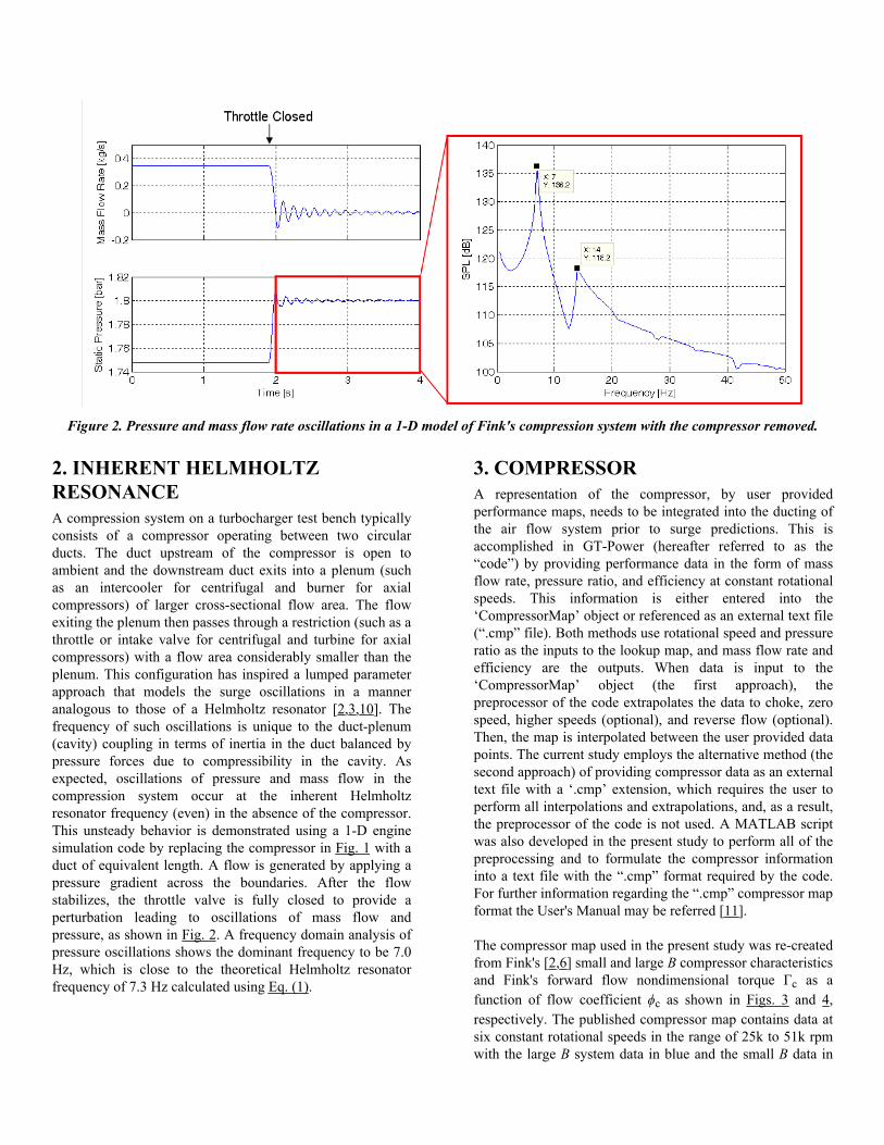
2. INHERENT HELMHOLTZRESONANCEA compression system on a turbocharger test bench typicallyconsists of a compressor operating between two circularducts. The duct upstream of the compressor is open toambient and the downstream duct exits into a plenum (suchas an intercooler for centrifugal and burner for axialcompressors) of larger cross-sectional flow area. The flowexiting the plenum then passes through a restriction (such as athrottle or intake valve for centrifugal and turbine for axialcompressors) with a flow area considerably smaller than theplenum. This configuration has inspired a lumped parameterapproach that models the surge oscillations in a manneranalogous to those of a Helmholtz resonator [2,3,10]. Thefrequency of such oscillations is unique to the duct-plenum(cavity) coupling in terms of inertia in the duct balanced bypressure forces due to compressibility in the cavity. Asexpected, oscillations of pressure and mass flow in thecompression system occur at the inherent Helmholtzresonator frequency (even) in the absence of the compressor.This unsteady behavior is demonstrated using a 1-D enginesimulation code by replacing the compressor in Fig. 1 with aduct of equivalent length. A flow is generated by applying apressure gradient across the boundaries. After the flowstabilizes, the throttle valve is fully closed to provide aperturbation leading to oscillations of mass flow andpressure, as shown in Fig. 2. A frequency domain analysis ofpressure oscillations shows the dominant frequency to be 7.0Hz, which is close to the theoretical Helmholtz resonatorfrequency of 7.3 Hz calculated using Eq. (1).

3. COMPRESSORA representation of the compressor, by user providedperformance maps, needs to be integrated into the ducting ofthe air flow system prior to surge predictions. This isaccomplished in GT-Power (hereafter referred to as the“code”) by providing performance data in the form of massflow rate, pressure ratio, and efficiency at constant rotationalspeeds. This information is either entered into the‘CompressorMap’ object or referenced as an external text file(“.cmp” file). Both methods use rotational speed and pressureratio as the inputs to the lookup map, and mass flow rate andefficiency are the outputs. When data is input to the‘CompressorMap’ object (the first approach), thepreprocessor of the code extrapolates the data to choke, zerospeed, higher speeds (optional), and reverse flow (optional).Then, the map is interpolated between the user provided datapoints. The current study employs the alternative method (thesecond approach) of providing compressor data as an externaltext file with a ‘.cmp’ extension, which requires the user toperform all interpolations and extrapolations, and, as a result,the preprocessor of the code is not used. A MATLAB scriptwas also developed in the present study to perform all of thepreprocessing and to formulate the compressor informationinto a text file with the “.cmp” format required by the code.For further information regarding the “.cmp” compressor mapformat the User's Manual may be referred [11].

The compressor map used in the present study was re-createdfrom Fink's [2,6] small and large B compressor characteristicsand Fink's forward flow nondimensional torque Γc as afunction of flow coefficient ϕc as shown in Figs. 3 and 4,respectively. The published compressor map contains data atsix constant rotational speeds in the range of 25k to 51k rpmwith the large B system data in blue and the small B data in

Figure 2. Pressure and mass flow rate oscillations in a 1-D model of Fink's compression system with the compressor removed.


red, as shown in Fig. 3. The “Large B Surge Line” (hereaftersimply referred to as the “surge line”) designates the deepsurge boundary for the large B compression system shown inFig. 1. To the right of the surge line, the small and large Bdata are identical, illustrating that the compressorcharacteristics are independent of the compression systemducting (a property of the compressor alone), yet the coupledcompression system (compressor, ducting, and throttle)dictates the stable portion of the map available for use. Thecompressor nondimensional torque Γc is calculated from mapdata as

(3)

where τc is the torque driving the compressor (Baines [12]),ρ0 is the density of air at ambient conditions, r2 is the radiusof the impeller tip, cp is specific heat of air at constantpressure, ṁc is the mass flow rate through the compressor, T1tis the total inlet temperature, ω is the angular velocity of theimpeller, PRc is the total-to-total pressure ratio of thecompressor, and γ is the ratio of specific heats. Thecompressor flow coefficient ϕc represents the mass flow ratenon-dimensionalized as

(4)

where ρ is the density at the compressor inlet (for forwardflow). The Γc vs. ϕc data shown in Fig. 4 provides aconvenient means for extrapolating compressor isentropicefficiency ηc to zero mass flow rate since the data at allrotational speeds nearly collapses onto a single curve.

The compressor characteristics of Fink are extrapolated hereto cover the entire forward flow operating region of thecompressor including down to zero speed, up to 60k rpm, tozero flow, and to choke. The pressure ratio of each constantspeed line at zero mass flow rate PR0 is calculated usingradial equilibrium theory and assuming an isentropic process[7]

(5)

Figure 3. Fink's small and large B compressorcharacteristics.

Figure 4. Fink's forward flow nondimensionalcompressor torque as a function of flow coefficient.

where CPR is a constant multiplier, R is the gas constant forair, and T1 is the compressor inlet temperature. r1 is the meangeometric radius of the impeller eye, which divides theimpeller eye area into two sections with the same area and iscalculated as

(6)

where r1,t and r1,h are the radii of the inducer tip and hub,respectively. For the present study, a CPR value slightly largerthan unity was applied to PR0 in Eq. (5) to match the


experimental data. This multiplier was 1.04 for the lowestspeed (25k rpm) and 1.09 for the highest compressor speed(51k rpm).

Since the rare small B system data is available for Fink'scompressor, the present study uses higher order polynomialsto fit the small B constant speed lines down to zero mass flowrate. This method allows the constant speed lines used in themodel to obtain a nearly perfect fit to the experimental data.If the rare small B system data were not available, the Mooreand Greitzer [13] method would have been used toextrapolate the compressor characteristics from the peakpressure rise to zero mass flow rate, as described in AppendixA.

The compressor map data must also be extrapolated down tozero speed, to choke, and optionally to higher speeds.Extrapolation to both lower and higher speeds is performedon the nondimensional characteristics. The compressor flowcoefficient ϕc is calculated using Eq. (4), and thenondimensional compressor isentropic head coefficientinvolves the nondimensional pressure as

(7)

where

(8)

p3t being the total pressure at the compressor exit and p0 thepressure at ambient conditions, and

(9)

is the compressor exit tip Mach number, with a0 being thespeed of sound at ambient conditions. Note that thenondimensional compressor characteristics (ψc vs. ϕc) nearlycollapse onto a single curve, partially removing the speeddependence, as shown in Fig. 5. The extrapolation of mapdata to lower speeds is achieved by performing a speedweighted linear interpolation between the nondimensionalform of the lowest constant speed line (25k rpm) and zerospeed, assuming zero mass flow rate, pressure rise, andefficiency when the impeller is not rotating. Extrapolation ofthe compressor data to higher speeds is completed bytransforming the nondimensional data of the highest constantspeed line (51k rpm) into dimensional form at higher speeds.The compressor data usually requires extrapolation to choke,but this procedure is neglected here since the range of

operation for the compressor in the current study is not nearthat region of the map.

Figure 5. Fink's nondimensional compressorcharacteristics.

A method similar to Theotokatos and Kyrtatos [7] is used toextrapolate the compressor efficiency down to zero mass flowrate. The nondimensional torque Γc vs. flow coefficient ϕcdata in Fig. 4 is extrapolated by applying a quadratic curve fitin the form

(10)

with C0-C2 being the fit constants. The extrapolatedcompressor efficiency is calculated by substituting Eq. (10)into Eq. (3) and using discrete values of ṁc and PRc from theextrapolated compressor characteristics. The compressor mapusually requires interpolation at intermediate speeds anddetails regarding the approach used in the current study areincluded in Appendix B.

The final version of the compressor map used for the code isshown in Fig. 6. The large and small B compression systemdata of Fink is superimposed on the map along with thecorresponding constant speed lines to illustrate thecomparison. The MATLAB script writes the compressor mapinformation to a text file with the required “.cmp” format.Since limited data is available for this compressor, thenondimensional torque (used to calculate efficiency) wasassumed to be independent of speed. As a result, thecompressor efficiency is only a factor of the flow coefficientat speeds above 25k rpm. This results in constant peakefficiency along each constant speed line. If more data wereto be available, Eq. (10) could be used to fit the Γc vs. ϕc dataat each constant speed individually and incorporate a speed-dependent efficiency.


Figure 6. Compressor map used for the current study.

4. ONE-DIMENSIONALCOMPRESSION SYSTEM MODELThe numerics describing unsteady, compressible fluid flowhave been incorporated into 1-D engine simulation codessince the late 1970's. The commercial code used here for thecurrent study solves the non-linear balance equations of mass,momentum and energy, along with the equation of state,using an explicit time integration method. These equationsare applied to spatially discrete control volumes within the airflow system. The 1-D mass conservation is represented by

(11)where m is the mass of the discrete volume, and ṁ is the massflow rate across the control volume boundaries. The 1-Dmomentum conservation may be expressed as

(12)where p is the pressure, A is the cross-sectional area of flow,u is the velocity at the boundary of the control volume, f thefriction coefficient, ρ is the density, D is the equivalentdiameter, and K is the pressure loss coefficient. The 1-Denergy conservation is expressed as

(13)

where e is the total internal energy (internal energy pluskinetic energy) per unit mass, V is the volume, h is thespecific enthalpy, hc is the heat transfer coefficient, As is theheat transfer area, Tf is the fluid temperature, and Tw is thewall temperature. The solutions of Eqs. (11), (12), (13) incombination with the equation of state yield the scalar fluidproperties within each control volume (pressure, temperature,density, internal energy, enthalpy, etc.) and the vectorproperties at the boundaries (mass flow rate, velocity, etc.).

The compression system of Fink is modeled in the code withthe compressor inlet pipe and throttle exit connected toambient boundary conditions. The compressor performancedata shown in Fig. 6 is input to the ‘Compressor’ object as atext file in “.cmp” format. Instead of incorporating a turbineinto the model, a drive torque is applied to the turbochargershaft for simplification. The turbocharger rotational inertia isoften artificially manipulated by use of a multiplier to speedup convergence of steady-state simulations. It is importantthat the inertia multiplier is maintained equal to onethroughout simulations near the surge line, as unsteady surgeoscillations may be encountered. This is especially importantfor turbocharged engine models where pressure pulsations inthe exhaust and induction systems cause speed fluctuations.

Among the options GT-Power offers for a time constant todampen changes in compressor mass flow rate, the presentstudy has chosen

(14)

This time constant is proportional to the time required for anumber of rotor revolutions n, and a value of n=2 is used inthe current study. If the damping is not present, a smallchange in pressure ratio at the peak of the characteristic cancause an unrealistically large change in mass flow rate in asingle time-step. This damping also allows the compressor todeviate from the steady-state map during unsteady surgecycles.

Incorporating surge prediction capabilities into a 1-D enginesimulation code offers the following benefits compared to thelumped parameter models of Greitzer [3] and Fink et al. [2]that have been used extensively in literature. First, thenonlinear formulation with spatial distribution allows thewave dynamics of the compression system to be modeled andis therefore advantageous for engine simulations. Second,many of the major simplifying assumptions required for thelumped parameter (0-D) model of Fink et al. can beeliminated, including: (a) incompressible flow in thecompressor duct, (b) isentropic plenum expansion orcompression, (c) choked throttle valve, (d) short throttle ductlength so that the inertia can be ignored, and (e) negligible


velocity in the plenum. A couple of the major simplifyingassumptions of the lumped parameter model that are retainedwithin the 1-D approach include: (a) discontinuity of pressureand density across the compressor, which is modeled as anactuator disk, and (b) negligible gas angular momentum inthe compressor passages compared to the impeller angularmomentum.

5. MILD SURGE SIMULATIONRESULTSThe simulations in the current study are aimed at reproducingthe experimental mild surge observations of Fink's [2,6] largeB compression system at a time average rotational speed of48k rpm (Mat,0=0.92). His data is shown in Fig. 7a withrepeating oscillations of the nondimensional parameters ϕc,Mat,0, and plenum isentropic head coefficient

(15)

where Πp is the ratio of total plenum pressure to ambientpressure. The ϕc data fluctuates with an amplitude of 20% ofthe mean flow (0.046) about a time mean value of 0.23, andthe dominant frequency of oscillations is reported as 7.3 Hz.

The compressor operating conditions on the surge line at 48krpm are ṁc =0.30 kg/s (ϕc=0.225) and PRc= 1.98 (ψc=0.637),and this marks the deep surge boundary of Fink'sexperimental results. For the simulations performed here, thecompressor is brought to a stable operating condition near thestability limit at 48k rpm. Then, the throttle at thecompression system exit is partially closed to move thecompressor operating point into the surge region. When thestability limit of the compression system is crossed, lowamplitude mild surge oscillations appear and grow to theconverged results presented in Fig. 7b for comparison withthe experimental results of Fink. For ease of suchcomparisons, Fig. 7b has retained both the horizontal andvertical axis scales the same as in Fig. 7a. The simulation isstopped when the cycle-to-cycle change in mass flow rateamplitude is extremely small (less than 1×10−5 kg/s here) toensure that the compression system does not enter deep surge.The oscillations of ϕc are predicted to occur at a mean valueof 0.22 with an amplitude of 0.046 (21% of the mean flow)and appear to be nearly identical to the results of Fink.Similarly, the Mat,0 and ψp predictions almost exactlyreproduce the amplitude, frequency, and the time averagedoperating point of the corresponding experimental results.These comparisons demonstrate the ability of nonlinear 1-Dtime-domain approaches to predict the compressor operatingconditions at the instability inception. Frequency-domainanalysis of the computed ϕc and ψp oscillations is shown in

Figure 7. Mild surge results: (a) Experimental data of Fink and (b) Simulation from the present study.


Fig. 8. The dominant fundamental frequency is predicted tobe 7.3 Hz, and the somewhat steepened wave forms lead toadditional frequency content at harmonics of the fundamentalfrequency. The predicted fundamental frequency is identicalto the measured result reported by Fink. The theoreticalHelmholtz resonance frequency may be calculated from Eq.(1) as

where the speed of sound is based on the mean plenumtemperature of 387 K. The equivalent duct length

is calculated using the compression system geometry in Fig. 1and taking the equivalent duct area (reference area) as thecross-sectional area of the inducer eye. The additionalfrequencies have also been observed experimentally byGravdahl et al. [14].

Figure 8. Frequency domain analysis of ϕc and ψp frommild surge simulation result.

The operating points of the compressor and plenum during asingle mild surge cycle are shown on the compressor map inFig. 9. Pressure ratios for both the compressor (PRc) and

plenum (PRp) are defined relative to the total pressure at thecompressor inlet. Mild surge operating points for thecompressor (PRc vs. ṁc in green symbols) oscillate in theclockwise direction on the map and the plenum (PRp vs. ̇mcin blue symbols) operates along a curved path. At Location 1of the compressor surge cycle, the operating point is nearlyon the peak of the 48k rpm characteristic. As ṁc and PRcdecrease, the operating points follow the constant speed lineand the surge line is crossed at Location 2. The mass flowrate and pressure ratio reach a minimum at Location 3, andthe compressor speed starts increasing. The compressor flowthen accelerates, back across the surge line, until the peakpressure ratio of the cycle is reached at Location 4. Then, thespeed and pressure ratio decrease to Location 1 and the cycleis repeated. The compressor and plenum operating pointshave uniformly spaced time intervals of 0.5 ms, making, forexample, the rate of change of ṁc and PRc clearly visible forthe compressor. Note that the discrete operating points arespaced further apart where the compressor mass flow isaccelerating, indicating that the compressor moves throughthis portion of the cycle at a rate faster than when the massflow rate is decelerating. During mild surge, the compressorspends a significant amount of time to the left of the surgeline. In order to predict mild surge, compressor performancedata is required in this region of the map where steady-statemeasurements are not obtainable with the large B system.This data must either be collected using a system with asmaller B number (as accomplished by Fink) or estimatedthrough extrapolation. The pressure ratio of the plenum (bluesymbols) is lower than that of the compressor because of thepressure losses in the intermediate ducting. The shape of theplenum surge cycles is essentially driven by the pressurewave at the Helmholtz resonator frequency.

Figure 10 shows the dimensionless compressor characteristicused in the present model with the data of Fink. Note that theflow coefficient ϕc on the surge line at 48k rpm is equal to0.225. Mild surge operating points in the compressor (ψc vs.ϕc in green symbols) and plenum (ψp vs. ϕc in blue symbols)oscillate in a counter-clockwise direction on thenondimensional compressor map. The change of compressorand plenum fluctuation shapes from dimensional (Fig. 9) tonondimensional (Fig. 10) maps is partially due to thedifferent definitions of nondimensional pressure and pressureratio. Π is relative to a constant reference pressure and is usedfor calculating ψc and ψp in Eqs. (7) and (15), respectively,while PR is relative to the fluctuating compressor inletpressure. The other factor contributing to the shape differenceis the fluctuating rotational speed, which appears as Mat,0 inthe denominator of Eqs. (4), (7), and (15). Mat,0 is largerwhen the compressor mass flow rate is accelerating (fromLocation 3 to 1 in Fig. 9) than when the mass flow rate isdecelerating (from Location 1 to 3 in Fig. 9). This contributesto a lower ψc during mass flow acceleration. The compressor


operating points nearly follow the nondimensionalcharacteristic while the flow is decelerating, but they operatebelow the steady-state map when accelerating. Thenondimensional plenum operating points follow an elliptical

path that appears to be nearly symmetrical about the surgeline.

Figure 9. Mild surge compressor and plenum operating points for a single cycle. Selected constant speed lines used in thepresent study and Fink's surge line are shown for reference.

Figure 10. Nondimensional mild surge compressor and plenum operating points for a single cycle. The nondimensional 48krpm speed line data of Fink et al. and the nondimensional compressor characteristic at 48k rpm (used in the model) are shown

for reference.


To gain further insight into the physics of mild surge, thepredicted static pressure, temperature, and mass flow rate aregiven at four locations within the compression system in Figs.11, 12, 13, respectively. Locations 1-3 and 7 are specified inFig. 1, corresponding to the mid-length of the compressorinlet duct, compressor inlet, compressor exit, and mid-lengthof the plenum, respectively. Figure 11 illustrates that thepressure fluctuations are most severe at the compressor inletwith an amplitude of approximately 2.2 kPa and least severeat the mid-length of the compressor inlet duct (among thelocations studied) with an amplitude of 0.25 kPa. Afrequency domain analysis of the pressure traces reveals thatthe maximum sound pressure level (SPL) of about 160 dBoccurs at the compressor inlet, corresponding to the dominantmild surge frequency (7.3 Hz), as shown in Fig. 14. Theharmonics of the Helmholtz resonances appear throughoutthe compression system due to non-linearity. It is expectedthat those harmonics above 20 Hz would become audible.The temperature fluctuations are largest at the compressorexit during mild surge, as shown in Fig. 12, but the amplitudeis relatively small at approximately 2.5 K. Mass flow ratefluctuations are severe throughout the compression system, asshown in Fig. 13. The large amplitude mass flow ratefluctuations at Locations 1-3 are nearly identical, and theamplitude in the plenum is lower due to smaller oscillationsin velocity as a result of the much larger cross-sectional areaof the plenum. The amplitude of mass flow rate oscillations atthe compressor is approximately 21% of the mean flow rate.Turbocharger rotational speed is shown to fluctuate with anamplitude of 175 rpm, and this is only 0.4% of the meanvalue, as shown in Fig. 15. The compressor efficiencyfluctuates between the peak value of 73% and about 67% inthe present study, as shown in Fig. 16.

Figure 11. Static pressure at compression systemlocations during mild surge.

Figure 12. Temperature at compression system locationsduring mild surge.

Figure 13. Mass Flow Rate at compression systemlocations during mild surge.

Figure 14. Sound pressure level at compression systemlocations during mild surge.


Figure 15. Shaft rotational speed during mild surge.

Figure 16. Compressor efficiency during mild surge.

6. INFLUENCE OF COMPRESSIONSYSTEM GEOMETRYThe compression system in Fig. 1 has a plenum length of2.38 m and a volume of 0.208 m3, resulting in B=2.7 (at 48krpm) and an instability inception point near the peak pressurerise of the compressor. As B decreases, the compressionsystem can operate free of surge at increasingly positivevalues of compressor characteristic slope (lower mass flowrates). For illustrative purposes, the volume of the plenum inFig. 1 is gradually reduced here to determine a critical Bvalue below which the compression system does not entersurge with the engine simulation code. The operatingconditions here are identical to those of Section 5, includingcompressor drive torque, valve diameter, boundaryconditions, and the geometry other than the plenum length. Aset of runs was performed by sweeping the value of B. Thepredictions reveal that reducing the plenum volume to 4.8%

(or, below) of that in Fig. 1 by essentially decreasing theplenum length to 0.115 m, hence B to 0.70 (or, below)eliminates the surge. The stable operating point of the B=0.70compression system is shown by the green dot in Fig. 17.Comparison of Figs. 9 and 17 demonstrates that a compressoroperating condition that has originally resulted in mild surgeoscillations can be stabilized by adequately reducing thevolume of the plenum (therefore B).

Figure 17. Stable operating point of the compressor witha decreased plenum length and B=0.70.

7. CONCLUSIONS• The present study has demonstrated the ability tosuccessfully predict compression system mild surge physicswith an unsteady nonlinear 1-D solver used in enginesimulations.

• The computational results obtained here for mild surgealmost exactly reproduce the amplitudes, frequency, and timeaveraged operating points of the experimental observations.

• For accurate mild surge modeling, it is desirable to employthe experimental data for the entire forward flow region ofthe compressor (from zero mass flow rate to choke). Whenexperimental data is not available, the compressorperformance must be estimated based on extrapolationtechniques. The present study implemented a compressormap which was created from experimental data that wasextrapolated and interpolated to cover the entire forward flowoperating region.

• The Theotokatos and Kyrtatos approach for estimation ofthe pressure ratio at zero mass flow rate is shown to provide asatisfactory agreement with experimental data, whilediffering slightly from the measurements at higher rotationalspeeds for the compressor studied.


• A detailed computational analysis of the pressure,temperature, and mass flow rate fluctuations is presented atkey compression system locations during mild surge.

• The instability inception point of the compressor is alsocomputationally determined, designating the stable operatinglimit.

• The approach described here may be incorporated intoturbocharged engine models to assist with the design.

REFERENCES1. Cumpsty, N.A., “Compressor Aerodynamics,” Krieger,Florida, ISBN 1-57524-247-8, 1989.

2. Fink, D.A., Cumpsty, N.A., and Greitzer, E.M., “SurgeDynamics in a Free-Spool Centrifugal Compressor System,”J. Turbomachinery 114:321-332, 1992.

3. Greitzer, E.M., “Surge and Rotating Stall in Axial FlowCompressors,” ASME J. Engineering for Power 98:190-197,1976.

4. Yano, T. and Nagata, B., “A Study on Surging Phenomenain Diesel Engine Air-Charging System,” The Japan Society ofMechanical Engineers 14:364-376, 1971.

5. Hansen, K.E., Jorgensen, P., and Larsen, P.S.,“Experimental and Theoretical Study of Surge in a SmallCentrifugal Compressor,” J. Fluids Engineering103:391-395, 1981.

6. Fink, D.A., “Surge Dynamics and Unsteady FlowPhenomena in Centrifugal Compressors,” Ph.D. thesis,Department of Aeronautics and Astronautics, MassachusettsInstitute of Technology, Cambridge, 1988.

7. Theotokatos, G. and Kyrtatos, N.P., “Diesel EngineTransient Operation with Turbocharger CompressorSurging,” SAE Technical Paper 2001-01-1241, 2001, doi:10.4271/2001-01-1241.

8. Galindo, J., Serrano, J. R., Climent, H., and Tiseria, A.,“Experiments and Modeling of Surge in Small CentrifugalCompressor for Automotive Engines,” Experimental Thermaland Fluid Sciences 32:818-826, 2008.

9. GT-Power (Version 7.0), Gamma Technologies Inc.,Westmont, IL, 2009.

10. Emmons, H. W., Pearson, C. E., Grant, H. P.,“Compressor Surge and Stall Propagation,” Transactions ofthe ASME 77:455-469, 1955.

11. Gamma Technologies Inc., “GT-Power User's Manual,”Version 7.0, 2009.

12. Baines, N.C., “Fundamentals of Turbocharging,”Concepts NREC, Vermont, ISBN 0-933283-14-8, 2005.

13. Moore, F.K. and Greitzer, E.M., “A Theory of Post-stallTransients in Axial Compression Systems. Part I:Development of Equations,” ASME J. Engineering for GasTurbines and Power 108:68-76, 1986.

14. Gravdahl, J.T., Willems, F., Jager, B., and Egeland, O.,“Modeling of Surge in Free-Spool Centrifugal Compressors:Experimental Validation,” J. of Propulsion and Power 20(5):849-857, 2004.

CONTACT INFORMATIONProf. Ahmet [email protected]

DEFINITIONS/ABBREVIATIONSa

Speed of sound

AArea of cross-section

AsSurface area for heat transfer

BNondimensional Greitzer number

CPRConstant multiplier

C0 − C2Curve fit constants

cpSpecific heat of air at constant pressure

DEquivalent diameter

dxLength of spatial discretization

eTotal internal energy per unit mass

ηIsentropic efficiency

fSkin friction coefficient


http://www.sae.org/technical/papers/2001-01-1241

http://dx.doi.org/10.4271/2001-01-1241

mailto:[email protected]

fHHelmholtz resonator frequency

γRatio of specific heats

ΓcNondimensional torque

hSpecific enthalpy

hcHeat transfer coefficient

KPressure loss coefficient

lDuct length

LcLength of equivalent compressor duct

mMass

ṁMass flow rate

Mat,0Mach number of impeller tip

nNumber of rotor revolutions

ωAngular velocity of the shaft

pPressure

ϕFlow coefficient

ΠNondimensional pressure

ψIsentropic head coefficient

PRPressure ratio (total-to-total)

PR0Pressure ratio at zero mass flow rate

RGas constant for air

r1Mean geometric radius of the impeller eye

r1,tRadius of the inducer tip

r1,hRadius of the inducer hub

r2Radius of the impeller tip

ρDensity

tTime

TTemperature

τcTorque absorbed by the compressor

τGTPTime constant

uVelocity


UVelocity of the impeller tip

VVolume

SUBSCRIPTS0 - 7

Location

cCompressor, convection

pPlenum

peakPeak pressure ratio

fFluid

tTotal property, tip

wWall


APPENDIX A

MOORE AND GREITZEREXTRAPOLATION METHODIf the small B compression system map data were notavailable, the Moore and Greitzer [13] constant speed lineextrapolation method would have been applied to the large Bdata from the peak pressure rise to zero mass flow rate. Thismethod is a cubic polynomial with PRc as a function of ṁcand is expressed as

(A1)

where PR0 is calculated using Eq. (8), PRpeak is the peakpressure ratio on the constant speed line, and ṁpeak is themass flow rate at PRpeak. Equation (A1) forces theextrapolation to pass through PR0 at zero mass flow rate andPRpeak at ṁpeak with zero slope at both locations. CombiningEqs. (8) and (Al), the large B compressor data is extrapolateddown to zero mass flow rate to evaluate the Moore andGreitzer method, as shown in Fig. A1. Equation (A1)somewhat underestimates PRc between the endpoints for thecompressor studied. Note again that the Moore and Greitzermethod was not used for the current study because custompolynomial fits to the small B data provided a better match.

Figure A1. Comparison of the Moore and Greitzerextrapolation method with Fink's small B experimental

data.

APPENDIX B

INTERPOLATION FORINTERMEDIATE ROTATIONALSPEEDSThe compressor data was interpolated at intermediate mapspeeds using the following methodology:

1. Each of the extrapolated constant speed line fits areevaluated with an equal number of points. These points aredistributed at the same normalized pressure ratio values foreach constant speed line, as shown in Fig. B1.

2. The points from two adjacent constant speed lines arenondimensionalized, as shown in Fig. B2.

3. A speed weighted linear interpolation is performedbetween corresponding points at the same normalizedpressure ratio.

4. The interpolated points are dimensionalized as mass flowrate and pressure ratio.

The compressor efficiency is interpolated using a similarprocedure.

Figure B1. Extrapolated constant speed lines with pointsat equal values of normalized PRc.


Figure B2. Nondimensional version of adjacent constantspeed lines.

The Engineering Meetings Board has approved this paper for publication. It hassuccessfully completed SAE's peer review process under the supervision of the sessionorganizer. This process requires a minimum of three (3) reviews by industry experts.

All rights reserved. No part of this publication may be reproduced, stored in aretrieval system, or transmitted, in any form or by any means, electronic, mechanical,photocopying, recording, or otherwise, without the prior written permission of SAE.

ISSN 0148-7191

doi:10.4271/2010-01-2142

Positions and opinions advanced in this paper are those of the author(s) and notnecessarily those of SAE. The author is solely responsible for the content of the paper.

SAE Customer Service:Tel: 877-606-7323 (inside USA and Canada)Tel: 724-776-4970 (outside USA)Fax: 724-776-0790Email: [email protected] Web Address: http://www.sae.orgPrinted in USA


http://dx.doi.org/10.4271/2010-01-2142

compression system published 10/25/2010

Documents