compressed dynamic mode decomposition for real-time object

arX

iv:1

512.

0420

5v1

[cs

.CV

] 1

4 D

ec 2

015

Compressed Dynamic Mode Decomposition for

Real-Time Object Detection

N. Benjamin ErichsonUniversity of St Andrews

Steven L. BruntonUniversity of Washington

J. Nathan KutzUniversity of Washington

Abstract

We introduce the method of compressive dynamic mode decomposition (cDMD) forrobustly performing real-time foreground/background separation in high-definition video.The DMD method provides a regression technique for least-square fitting of video snap-shots to a linear dynamical system. The method integrates two of the leading data analysismethods in use today: Fourier transforms and Principal Components. DMD modes withtemporal Fourier frequencies near the origin (zero-modes) are interpreted as background(low-rank) portions of the given video frames, and the terms with Fourier frequenciesbounded away from the origin are their foreground (sparse) counterparts. When com-bined with compression techniques, the resulting cDMD can process full HD video feedsin real-time on CPU computing platforms while still maintaining competitive video decom-position quality, quantified by F-measure, Recall and Precision. On a GPU architecture,the method is significantly faster than real-time, allowing for further video processing toimprove the separation quality and/or enacting further computer vision processes such asobject recognition.

Keywords: dynamic mode decomposition, compressed sensing, object detection, backgroundsubtraction, video surveillance, robust principal component analysis.

1. Introduction

One of the most fundamental computer vision objectives is to detect moving objects in a givenvideo stream. This is especially critical for surveillance and/or target tracking applicationswhere accurate and real-time analysis must be accomplished. At the most basic level, dynamicpixels/objects in successive video frames are considered foreground objects whereas staticpixels/objects are considered part of the background. Thus the foreground can be foundin a video by removing the background, a challenging task that has been of long-standinginterest in the computer vision community. This task is also known as foreground-backgroundseparation and/or background modeling. One of the great challenges in this field is to performthe separation task with HD quality video streams in real-time, something that is at the edgeof performance limits for state-of-the-art algorithms. We integrate two recent innovations,the dynamic mode decomposition (DMD) [1] and compressive DMD (cDMD) [2] in order toachieve the goal of video analysis in real-time for HD quality streams. The methods takeadvantage of dynamical systems theory and recent developments in compressive sensing andsparsity. The results are compared against several leading methods, showing remarkableperformance gains in computation time.

http://arxiv.org/abs/1512.04205v1

2 Compressed Dynamic Mode Decomposition for Real-Time Object Detection

Algorithms for performing foreground/background separation face a number of performancechallenges. Competitive methods often need to be flexible enough to accommodate changesin a scene due to, for instance, illumination changes that can occur throughout the day, orlocation changes where the application is being implemented. Indeed, the list of deleteriouseffects incurred in video processing are significant and include camera jitter, camera auto-matic adjustments, illumination changes, dynamic backgrounds, shadows, multiple movingforeground objects, etc. To be more precise, it is extremely rare that the camera is fixed,the background is static, only a single foreground object is present, and the illumination isconstant and adequate. As such, there is no single method currently available that is capableof handling all the challenges in real videos without suffering performance failures.

Given the importance of this task for video analysis, a variety of mathematical methods andalgorithms have been developed over the past decade and a half in order to perform back-ground/foreground separation. Some of the earliest techniques developed statistical, machinelearning methods for the separation process [3, 4, 5, 6], including a method based upon prin-cipal component analysis (PCA) [7]. More recent innovations have centered around low-rankand sparse matrix decompositions, or robust principal component analysis (RPCA) [8, 9, 10,11, 12, 13], a theoretical viewpoint we will build upon with the DMDmethodology. Indeed, theDMD algorithm can be shown to provide an effective way to perform an RPCA [14, 15]. So al-though the literature on background subtraction is immense, our focus is on these later RPCA-like techniques. However, we point the reader to several recent reviews [16, 17, 18, 19, 20]and a textbook [21] which highlight many of the methods developed and their performancemetrics. Further, we direct the interested reader to the Background Subtraction website [22]which provides a comprehensive list of methods and algorithms and their relative performanceon canonical data sets.

1.1. Related work

One common viewpoint of this computational task that relates closely with our method, isas a matrix separation problem into low-rank (background) and sparse (foreground) compo-nents [17, 21]. This viewpoint has been advocated, for instance, by Candes et al. in the frame-work of robust principal component analysis (RPCA) [11], and it has been extended to recentsubspace tracking algorithms for foreground/background separation algorithms [20, 23, 24].Thus, given a collection of data from a video stream, the RPCA method will seek out thesparse structures (foreground objects) within the data, while simultaneously fitting the re-maining entries to a low-rank basis (static background). As long as the given data is trulyof this nature, in that it lies on a low-dimensional subspace and has sparse components, thenthe RPCA algorithm has been proven by Candes et al. [11] to perfectly separate the givendata X according to

X = L+ S (1)

where L is low-rank and S is sparse.

Key to achieving such a matrix decomposition is ℓ1 optimization. By weighting a combinationof the nuclear and the ℓ1 norms, a convenient convex optimization problem called principal

component pursuit (PCP) was demonstrated, under suitable assumptions, to recover the low-rank and sparse components exactly of a given data-matrix (or video for our purposes). Thus

N. Benjamin Erichson, Steven L. Brunton, J. Nathan Kutz 3

the mathematical framework that enables PCP is given by [11]

minL,S‖L‖∗ + λ‖S‖1 subject to X− L− S = 0. (2)

where ‖ · ‖∗ and ‖ · ‖1 are the nuclear and ℓ1 norms respectively, and λ > 0 is an arbitrarybalance parameter that is typically chosen to be λ = 1/

√

max(n,m); here X is an n × mmatrix. This RPCA technique, which has its computational costs dominated by the convexoptimization procedure, was shown to be highly-competitive in comparison to the state-of-the-art computer vision procedure developed by De La Torre and Black [12] which is basedupon principal component analysis [7].

The PCP concept (2) is mathematically sound and has been successful for video processing.Its biggest challenge is computational speed and efficiency, especially given the iterative natureof the optimization required. Indeed, modern efforts around PCP have focused primarily onalgorithms that overcome the computational complexity of the original algorithm. For athorough discussion of such methods, see the recent review of Bouwmans and Zahzah [20].This review article highlights the state-of-the-art in performing RPCA separation using thePCP framework. It also gives a comprehensive review of performance on video processingtasks, from accuracy to speed. Additionally, it compares the PCP-based methods against oneof the leading mixture of Gaussians background models [3, 19].

1.2. Contribution

In this manuscript, we advocate a similar matrix decomposition approach, but by using themethod of dynamic mode decomposition (DMD) [25, 26, 27, 28] instead of RPCA [11]. Thismethod, which essentially implements a Fourier decomposition of the video frames in time, dis-tinguishes the stationary background from the dynamic foreground by differentiating betweenthe near-zero modes and the remaining modes bounded away from the origin, respectively.Originally introduced in the fluid mechanics community, DMD has emerged as a powerfultool for analyzing the dynamics of nonlinear systems [25, 26, 27, 28]. In the context of fluids,DMD has gained popularity since it provides, in an equation-free manner, information aboutthe dynamics of flow even if the underlying dynamics are nonlinear. It is equation-free in thesense that a typical application requires collection of a time series of experimental (or simu-lated) velocity field data, from which DMD modes and eigenvalues are computed. The modesare spatial fields that often identify coherent structures in the flow. The corresponding eigen-values define growth/decay rates and oscillation frequencies for each mode. More precisely,the DMD provides a regression to the least-square fit linear dynamical system modeling thedata snapshots collected [28]. Taken together, the DMD modes and eigenvalues describe thedynamics observed in the time series in terms of growth, decay, and oscillatory components;i.e. it decomposes data into Fourier modes in time [29].

In the application of video surveillance, the video frames can be thought of as snapshots ofsome underlying complex/nonlinear dynamics. The DMD yields oscillatory time componentsof the video frames that have contextual implications. Namely, those modes that have eigen-values near the origin represent dynamics that are unchanging, or changing slowly, and canbe interpreted as stationary background pixels, or low-rank components of the data matrix.In contrast, those modes bounded away from the origin are changing on O(1) timescales orfaster, and represent the foreground motion in the video, or the sparse components of thedata matrix. Thus, by simply applying the dynamical systems interpretation of DMD to


video frames, an approximate RPCA technique can be enacted at a fixed cost of a singular-value decomposition and a linear equation solve. Unlike the convex optimization procedureof Candes et al. [11], which can be guaranteed to exactly produce a low-rank and sparseseparation under certain assumptions, no such guarantees are currently given for the DMDprocedure. Regardless, in comparison with the RPCA [11] and computer vision [12] methods,the DMD procedure is orders of magnitude faster in computational performance since it relieson only a single singular value decomposition, resulting in real-time separation on laptop-classcomputing power, which suggests that this DMD technique merits serious consideration. Itshould be noted however, that recent advances in optimization (principal component pursuit,for instance), allows for significant improvement in computing the matrix decompositionsnecessary for this background separation task [17].

2. Background

2.1. Dynamic Mode Decomposition (DMD)

DMD is an equation-free, data-driven matrix decomposition that is capable of providing ac-curate reconstructions of spatio-temporal coherent structures arising in nonlinear dynamicalsystems, or short-time future estimates of such systems. DMD traces its origins to BernardKoopman in 1931 [30]. However, it had limited early impact since computers had not yetbeen invented and only analytic results, for simple problems, could be obtained. The work ofKoopman was revived by Mezic and co-workers starting in 2004 [31, 32], when both moderncomputers and a deep theoretical understanding of dynamical systems theory was available.In short, Koopman theory is a dynamical systems tool that provides complete informationabout a nonlinear dynamical system via an associated infinite-dimensional linear operator.Specifically, it provides a theoretical characterization that is readily interpretable in terms ofstandard methods of dynamical systems.

DMD is a special case of Koopman theory where the so-called Koopman observables arejust the state space itself [33]. Specifically, Schmid [25] proposed the DMD architecture formodeling complex flows. The connection with Koopman theory was only made theoreticallyrigorous by the subsequent work of Rowley et al. [26]. The connection between the works ofMezic, Schmid and Rowley and their co-workers between 2004-2010 laid the foundations forDMD as a transformative mathematical architecture. Indeed, in the last few years alone, DMDhas seen tremendous development in both theory and application. In theory, DMD has seeninnovations around sparsity [34] and compressive architectures [35, 2, 36], multi-resolutionanalysis [37], control theory [38], robust principal components analysis (RPCA) [14, 15], andde-noising algorithms [39, 40]. In addition to continued progress in fluid dynamics, DMD hasbeen applied to new domains, including neuroscience [41], epidemiology [42], robotics [43],and the current application of video processing and computer vision [1, 44, 14, 15].

In what follows, we use the most recent formal definition of the DMD method [27]:

Definition: Dynamic Mode Decomposition (Tu et al. 2014 [27]): Suppose we have two


sets of data

X=

x1 x2 · · · xm

, X′=

x′1 x′

2 · · · x′m

(3)

where each column xk of X is an initial condition and each column x′k of X′ is the corre-

sponding output after some prescribed evolution time ∆t with there being m initial conditions

considered. The DMD modes are eigenvectors of

A = X′X† (4)

where † denotes the Moore-Penrose pseudoinverse.

The definition of DMD thus yields the matrix A, which is a finite dimensional approximationof the Koopman operator for a linear observable.

At its core, the DMD is a regression algorithm. Specifically, it produces a regression to thebest-fit linear dynamical system for the data X. The DMD procedure thus constructs theproxy, approximate linear evolution

xk+1 = Axk. (5)

The eigenvalues λj and eigenvectors φj of A characterize the system dynamics. This inducesan associated continuous-time dynamical system given by

dx

dt= Ax, (6)

with A = exp(A∆t). For an initial condition x(0) = x0, the solution of Eq. (6) is given by

x(t) =

k∑

j=1

bjφj exp(ωjt) , (7)

where ωj = log(λj)/∆t are the continuous-time eigenvalues. The ultimate goal in the DMDalgorithm is to optimally construct the matrix A so that the true and approximate solutionsremain optimally close in a least-square sense:

‖x(t)− x(t)‖ ≪ 1. (8)

Of course, the optimality of the approximation holds only over the sampling window whereA is constructed, but the approximate solution can be used to not only make future statepredictions, but also to decompose the dynamics into various time-scales since the ωj areprescribed. Moreover, the DMD typically makes use of low-rank structure so that the totalnumber of modes, k ≪ n, allows for dimensionality reduction of the complex system or videostream.

In practice, when the state dimension n is large, the matrix A may be intractable to analyzedirectly. Instead, DMD circumvents the eigendecomposition of A by considering a rank-reduced representation in terms of a PCA-projected matrix A. The DMD algorithm proceedsas follows [27]:


1. Compute the SVD of X[45]:X = UΣV∗, (9)

where ∗ denotes the conjugate transpose, U ∈ Cn×k, Σ ∈ C

k×k and V ∈ Cm−1×k. Here

k is the rank of the reduced SVD approximation to X. The left singular vectors U areessentially PCA modes.

The SVD reduction in (9) could also be exploited at this stage in the algorithm toperform a low-rank truncation of the data. Specifically, if low-dimensional structure ispresent in the data, the singular values of Σ will decrease sharply to zero with perhapsonly a limited number of dominant modes. A principled way to truncate noisy datawould be to use the recent hard-thresholding algorithm of Gavish and Donoho [46].

2. Next, compute A, the k × k projection of the full matrix A onto POD modes:

A = X′VΣ−1U∗

=⇒ A = U∗AU = U∗X′VΣ−1. (10)

3. Compute the eigendecomposition of A:

AW = WΛ, (11)

where columns of W are eigenvectors and Λ is a diagonal matrix containing the cor-responding eigenvalues λj . Recall that the continuous-time eigenvalues are given byωj = log(λj)/∆t.

4. Finally, we may reconstruct eigendecomposition of A from W and Λ. In particular, theeigenvalues of A are given by Λ and the eigenvectors of A (DMD modes) are given bycolumns of Φ:

Φ = X′VΣ−1W. (12)

Note that Eq. (12) from [27] differs from the formula Φ = UW from [25], although these willtend to converge if X and X′ have the same column spaces.

2.2. Application to Video

The DMD algorithm applies to generic, time-dependent data. Our interest in this work is toconnect it to computer vision and video processing applications [1, 44, 14, 15]. For video, thedata collection process involves two parameters:

n = number of pixels saved per time snapshot,

m+ 1 = number of video frames (snapshots) taken.

The video snapshots are arranged into two n × m matrices X and X′ defined in the DMDalgorithm.

A video sequence offers an appropriate application for DMD because the frames of thevideo are, by nature, equally spaced in time, and the pixel data, collected in every snap-shot, can readily be vectorized. Given m + 1 frames of the video stream, the n × 1 vectorsx1,x2, . . . ,xm+1 can be extracted, which contain the pixel data of each frame; there being


n pixels in total per frame. The DMD method can attempt to reconstruct any given frame,or even possibly future frames, by calculating xDMD(t) at the corresponding time t via theDMD algorithm. The validity of the reconstruction depends on how well the specific videosequence meets the assumptions and criteria of the DMD method.

In order to reconstruct the entire video, consider the 1×m+1 time vector t = [t1 t2 . . . tm+1],which contains the times at which the frames were collected. If tj = j − 1 ∀j, then timebecomes equivalent to the frame count, where the first frame is labelled as 0 and the lastframe is labelled as m. The video sequence X and X′ are reconstructed with the DMDapproximation (7). Notice that the DMD mode φk is a n×1 vector which is used to constructan n×m video at each point of the time vector t using (7). By the construction of the DMDmethodology: x1 = Φb, which means that Φb renders the first frame of the video with adimensionality reduction chosen through the parameter k.

It becomes apparent that any portion of the first video frame that does not change in time, orchanges very slowly in time, must have an associated eigenvalue (ωj) that is located near theorigin in complex space: ‖ωj‖ ≈ 0. This fact becomes the key principle that makes possiblethe ability of the DMD method to separate background (approximate low-rank) informationfrom foreground (approximate sparse) information.

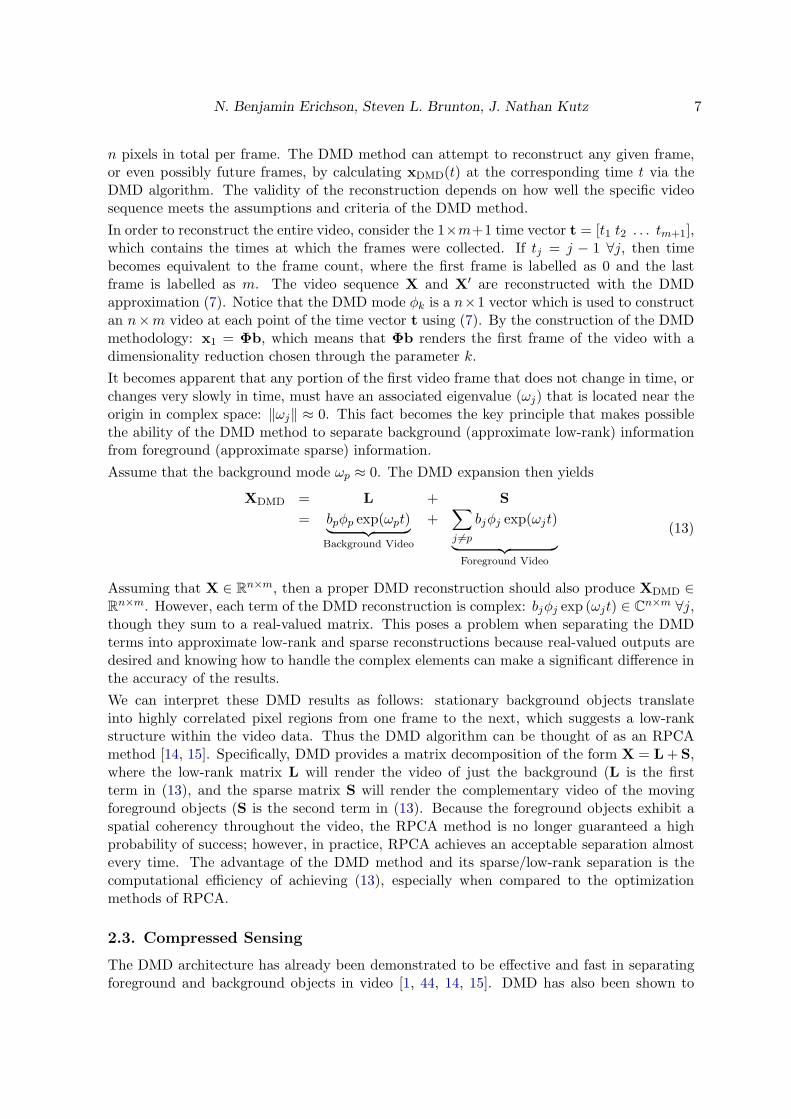
Assume that the background mode ωp ≈ 0. The DMD expansion then yields

XDMD = L + S

= bpφp exp(ωpt)︸︷︷︸

Background Video

+∑

j 6=p

bjφj exp(ωjt)

︸︷︷︸

Foreground Video

(13)

Assuming that X ∈ Rn×m, then a proper DMD reconstruction should also produce XDMD ∈

Rn×m. However, each term of the DMD reconstruction is complex: bjφj exp (ωjt) ∈ C

n×m ∀j,though they sum to a real-valued matrix. This poses a problem when separating the DMDterms into approximate low-rank and sparse reconstructions because real-valued outputs aredesired and knowing how to handle the complex elements can make a significant difference inthe accuracy of the results.

We can interpret these DMD results as follows: stationary background objects translateinto highly correlated pixel regions from one frame to the next, which suggests a low-rankstructure within the video data. Thus the DMD algorithm can be thought of as an RPCAmethod [14, 15]. Specifically, DMD provides a matrix decomposition of the form X = L+ S,where the low-rank matrix L will render the video of just the background (L is the firstterm in (13), and the sparse matrix S will render the complementary video of the movingforeground objects (S is the second term in (13). Because the foreground objects exhibit aspatial coherency throughout the video, the RPCA method is no longer guaranteed a highprobability of success; however, in practice, RPCA achieves an acceptable separation almostevery time. The advantage of the DMD method and its sparse/low-rank separation is thecomputational efficiency of achieving (13), especially when compared to the optimizationmethods of RPCA.

2.3. Compressed Sensing

The DMD architecture has already been demonstrated to be effective and fast in separatingforeground and background objects in video [1, 44, 14, 15]. DMD has also been shown to


Figure 1: Compressed sensing measurement process.

be effective when using a compression architecture [2]. Our goal is to combine these twomethods to provide a transformationally fast algorithm for video processing and computervision applications. Indeed, compression algorithms are at the core of modern video, imageand audio processing software such as MPEG, JPEG and MP3.

In our mathematical infrastructure of cDMD, we consider the theory of compressed sensingas developed from 2006 onwards [47, 48, 49, 50, 51, 52]. It demonstrates that instead ofmeasuring the high-dimensional signal, or pixel space representation of a single frame x, wecan measure instead a low-dimensional subsample y and approximate/reconstruct the fullstate space x with this significantly smaller measurement. Specifically, compressive sensingassumes the data being measured is compressible in some basis, which is certainly the casefor video. Thus the video can be represented in a small number of elements of that basis, i.e.we only need to solve for the few non-zero coefficients in the transform basis. For instance,consider the measurements y ∈ R

p, with k < p≪ n:

y = Cx,

as shown in Fig. 1. The measurement matrix C is often denoted by Φ in the compressedsensing literature. However, Φ is already used to represent DMD modes.

If x is sparse in Ψ, then we may solve the underdetermined system of equations

y = CΨs (14)

for s and then reconstruct x. Since there are infinitely many solutions to this system ofequations, we seek the sparsest solution s. However, it is well known from the compressivesensing literature that solving for the sparsest solution formally involves an ℓ0 optimizationthat is NP-hard and computationally intractable. The success of compressive sensing is thatit ultimately engineered a solution around this issue by showing that one can instead, undercertain conditions on the measurement matrix C, trade the infeasible ℓ0 optimization for aconvex ℓ1-minimization [50, 47]:

s = argmins′

‖s′‖1, such that y = CΨs′. (15)

Thus the ℓ1-norm acts as a proxy for sparsity promoting solutions of s.

To guarantee that the compressive sensing architecture will almost certainly work in a prob-abilistic sense, the measurement matrix C and sparse basis Ψ must be incoherent, meaningthat the rows of C are uncorrelated with the columns of Ψ. Incoherence is quantified by the


function µ(C,Ψ):

µ(C,Ψ) =√nmax

i,j|〈cj ,ψi〉|,

where cj is the j-th row of C and ψi is the i-th column of Ψ.

For incoherent measurements, the matrix CΨ satisfies a restricted isometry property (RIP),so it acts like an isometry map on sparse vectors s,

(1− δk)‖s‖22 ≤ ‖CΨs‖22 ≤ (1 + δk)‖s‖22, (16)

where δk is the restricted isometry constant [53]. This constant δk is the smallest numberthat satisfies Eq. (16) for all k-sparse vectors s. For small δk, the map CΨ acts as a nearisometry on k-sparse vectors s, so that distances and angles are preserved between sparsevectors. It is difficult to compute δk directly, and we generally prefer a statistical descriptionof the bounds on δk since C will be randomly generated. Typically, increasing the number ofmeasurements will decrease the restricted isometry constant δk, thus making CΨ closer to anisometry on sparse vectors. On the order of k log(n/k) measurements must be acquired fora δk that enables exact reconstruction of the k nonzero elements of the n-length vector s fornoiseless data [54, 48, 51]. An in-depth discussion of incoherence and the RIP can be foundin [51, 53]. The restricted isometry property of CΨ will facilitate compressed dynamic modedecomposition for data with low-rank structure.

Given that we are considering video images, it is easy to suggest the use of generic basisfunctions such as Fourier or wavelets in order to represent the sparse signal s. Indeed, waveletsare already the standard for image compression architectures such as JPEG-2000. As forthe Fourier transform basis, it is particularly attractive for many engineering purposes sincesingle-pixel measurements are clearly incoherent given that it excites broadband frequencycontent. If an image is k-sparse in the Fourier domain, we may then reconstruct the fullimage from O(k log(n/k)) single-pixel measurements at random spatial locations. In additionto Fourier and wavelet basis functions, compressive sensing has shown that Bernouli andGaussian random measurement matrices C satisfy the RIP property with high probabilityfor a generic basis Ψ [49]. There is also work describing incoherence with sparse matricesand generalizations to the RIP [55]. More optimally, one can pair the compressive sensingscheme with a data-driven POD/PCA basis, in which the data is optimally (in an ℓ2-sense)sparse [28, 56, 57, 58, 59]. The use of a POD/PCA basis results in a more computationallyefficient signal reconstruction from even fewer measurements.

More generally, there have been a significant number of innovations around sparsity and sparserepresentation using ℓ1 minimization and/or greedy algorithms [60, 61, 62, 63] that iterativelydetermine sparse solutions to the underdetermined system in Eq. (14). The compressionideology is also critical for producing efficient algorithms associated with compressed SVDand PCA computations based on the Johnson-Lindenstrauss (JL) lemma [64, 65, 66, 63]. TheJL lemma is closely related to the RIP, and it states when it is possible to embed a set ofhigh-dimensional vectors in a low-dimensional space while preserving the spectral properties.

3. Compressed DMD (cDMD)

Compressed DMD provides a computationally efficient framework to compute the dynamicmode decomposition on massively under-sampled or compressed data [2]. The method was


X,X′ ΦX,ΛX

Y,Y′ ΦY,ΛY

DMD

cDMD

C Eq. (24)

Data Dynamic Modes

Full

Compressed

Figure 2: Schematic illustrating the compressed DMD architecture. Full data is firstcompressed via left multiplication by a compression matrix C. Next, DMD is performed onthe compressed data. Finally, full DMD modes ΦX may be reconstructed from compressed

modes ΦY by the expression in Eq. (24).

originally devised to reconstruct high-dimensional, full-resolution DMD modes from sparse,spatially under-resolved measurements by leveraging compressed sensing. However, it wasquickly realized that if full-state measurements are available, many of the computationallyexpensive steps in DMD may be computed on a compressed representation of the data, pro-viding dramatic computational savings. The first approach, where DMD is computed onsparse measurements without access to full data, is referred to as compressed sensing DMD

(csDMD). The second approach, where DMD is accelerated using a combination of calcula-tions on compressed data and full data, is referred to as compressed DMD (cDMD); this isdepicted schematically in Fig. 2. For the applications explored in this work, we use the com-pressed DMD, since full image data is available and reducing algorithm run-time is criticalfor real-time performance.

3.1. Algorithm

For both compressed DMD (cDMD) and compressed sensing DMD (csDMD), we considercompressed measurements y that are related to the full image x by:

y = Cx. (17)

Again, the matrix C ∈ Rp×n compresses or sub-samples the data in x. These compressed

measurements are stacked as the columns of data matrices as in Eq. (3):

Y = CX, Y′ = CX′. (18)

There is a fundamental assumption that each of the columns of X and X′ are sparse in sometransform basis Ψ, so that X = ΨS and X′ = ΨS′. Thus, for sufficiently many incoherentmeasurements, the compressed matrices Y and Y′ have similar correlation structures to


their high-dimensional counterparts, as in the compressed sensing discussion above. This isdiscussed in more detail in [2].

The compressed DMD algorithm proceeds similarly to full-state DMD at nearly every stepuntil the computation of the DMD modes. Compressed DMD approximates the eigenvaluesand eigenvectors of the linear map AY defined as:

AY = Y′Y† (19a)

= Y′VYΣ−1Y

UY∗, (19b)

where the pseudo-inverse Y† is computed using the SVD:

Y = UYΣYVY∗. (20)

Note that the subscript Y is included to explicitly denote computations and data obtainedfrom the compressed data Y. As in the standard DMD algorithm, we typically do notcompute the large matrix AY, but instead compute the low-dimensional model projectedonto POD/PCA modes:

AY = UY∗AYUY (21a)

= UYY′VYΣ−1Y

. (21b)

The eigendecomposition of AY yields

AYWY = WYΛY, (22)

and the compressed DMD modes are given by

ΦY = Y′VYΣ−1Y

WY. (23)

To obtain full-state DMD modes, we may either apply compressed sensing to each mode inΦY, which would be compressed sensing DMD, or we may apply the linear transformationsobtained using Y and Y′ to the full-state data X′:

ΦX = X′VYΣ−1Y

WY. (24)

Note that the compressed DMD modes in Eq. (24) make use of the full data X′ as well as thelinear transformations obtained using the compressed data Y and Y′. The expensive SVDon X is bypassed, and it is instead performed on Y. Depending on the compression ratio,this may provide significant computational savings.

The compressed DMD computation is described in Algorithm 1, and more theoretical andnumerical details about the compressed DMD architecture are provided in 3. However, it isimportant to note that many fewer measurements may be used in compressed DMD than incompressed sensing DMD. In a variety of examples, as few as O(10)−O(100) measurementswere sufficient to yield excellent compressed DMD eigenvalues and modes. There are a fewconditions on the data and compression that must be met for compressed DMD to work, butin practice these are less stringent than the requirements for compressed sensing. In addition,examples indicate that fewer compressed measurements are required to resolve low-frequencyDMD modes, such as the zero-frequency background mode.


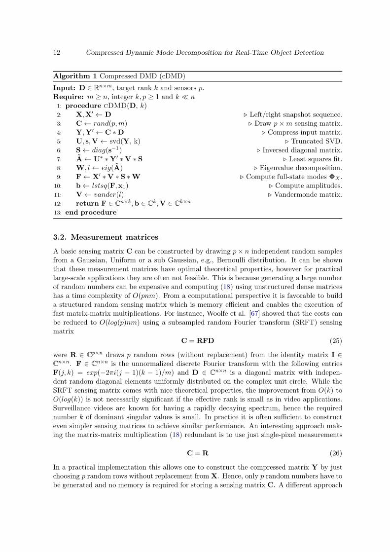
Algorithm 1 Compressed DMD (cDMD)

Input: D ∈ Rn×m, target rank k and sensors p.

Require: m ≥ n, integer k, p ≥ 1 and k ≪ n1: procedure cDMD(D, k)2: X,X′ ← D ⊲ Left/right snapshot sequence.3: C← rand(p,m) ⊲ Draw p×m sensing matrix.4: Y,Y′ ← C ∗D ⊲ Compress input matrix.5: U, s,V ← svd(Y, k) ⊲ Truncated SVD.6: S← diag(s−1) ⊲ Inversed diagonal matrix.7: A← U∗ ∗Y′ ∗V ∗ S ⊲ Least squares fit.8: W, l ← eig(A) ⊲ Eigenvalue decomposition.9: F← X′ ∗V ∗ S ∗W ⊲ Compute full-state modes ΦX .

10: b← lstsq(F,x1) ⊲ Compute amplitudes.11: V← vander(l) ⊲ Vandermonde matrix.12: return F ∈ C

n×k,b ∈ Ck,V ∈ C

k×n

13: end procedure

3.2. Measurement matrices

A basic sensing matrix C can be constructed by drawing p× n independent random samplesfrom a Gaussian, Uniform or a sub Gaussian, e.g., Bernoulli distribution. It can be shownthat these measurement matrices have optimal theoretical properties, however for practicallarge-scale applications they are often not feasible. This is because generating a large numberof random numbers can be expensive and computing (18) using unstructured dense matriceshas a time complexity of O(pnm). From a computational perspective it is favorable to builda structured random sensing matrix which is memory efficient and enables the execution offast matrix-matrix multiplications. For instance, Woolfe et al. [67] showed that the costs canbe reduced to O(log(p)nm) using a subsampled random Fourier transform (SRFT) sensingmatrix

C = RFD (25)

were R ∈ Cp×n draws p random rows (without replacement) from the identity matrix I ∈

Cn×n. F ∈ C

n×n is the unnormalized discrete Fourier transform with the following entriesF(j, k) = exp(−2πi(j − 1)(k − 1)/m) and D ∈ C

n×n is a diagonal matrix with indepen-dent random diagonal elements uniformly distributed on the complex unit circle. While theSRFT sensing matrix comes with nice theoretical properties, the improvement from O(k) toO(log(k)) is not necessarily significant if the effective rank is small as in video applications.Surveillance videos are known for having a rapidly decaying spectrum, hence the requirednumber k of dominant singular values is small. In practice it is often sufficient to constructeven simpler sensing matrices to achieve similar performance. An interesting approach mak-ing the matrix-matrix multiplication (18) redundant is to use just single-pixel measurements

C = R (26)

In a practical implementation this allows one to construct the compressed matrix Y by justchoosing p random rows without replacement from X. Hence, only p random numbers have tobe generated and no memory is required for storing a sensing matrix C. A different approach


ALU ALU

ALU ALU

Control

L2

DRAM

(a) CPU

L2

DRAM

(b) GPU

Figure 3: Illustration of the CPU and GPU architecture.

is the method of sparse random projections [68]. The idea is to construct a sensing matrix C

with identical independent distributed entries as follows

cij =

1 with prob. 12s

0 with prob. 1− 1s

-1 with prob. 12s

(27)

where the parameter s controls the sparsity. While Achlioptas [68] has proposed the valuess = 1, 2, Li et al. [69] showed that also very sparse (aggressive) sampling rates like s =n/log(n) achieve accurate results. Hence, using a modern sparse matrix package allows arapid execution of (18).

If available, domain specific knowledge can also be utilized to construct the measurementmatrix. This allows for more flexibility and makes the approach using compressed sensinginteresting and feasible for many domain specific applications.

3.3. GPU Accelerated Implementation

While most current desktop computers allow multithreading and also multiprocessing, using agraphics processing unit (GPU) enables massive parallel processing. The paradigm of parallelcomputing becomes more important with increasingly large amounts of data and stagnatingCPU clock speeds. The architecture of a modern CPU and GPU is illustrated in Figure 3.The key difference between these architectures is that the CPU consists of few arithmeticlogic units (ALU) and is highly optimized for low-latency access to cached data sets, whilethe GPU is optimized for data-parallel, throughput computations. This is achieved by thelarge number of small arithmetic logic units (ALU).

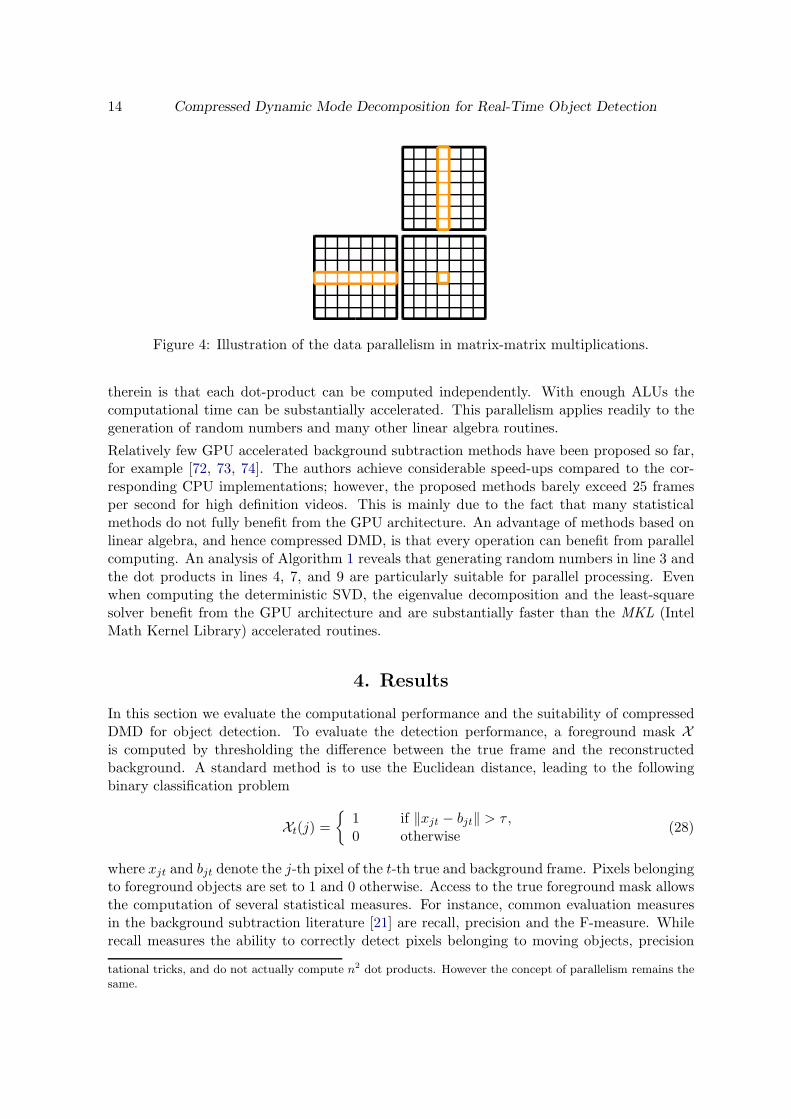
Traditionally this architecture was designed for the real-time creation of high-definition 2D/3Dgraphics. However, NVIDIA’s programming model for parallel computing CUDA opens upthe GPU as a general parallel computing device [70]. Using high-performance linear algebralibraries, e.g. CULA [71], can help to accelerate comparable CPU implementations substan-tially. Take for instance the matrix multiplication of two n×n square matrices, illustrated inFigure 4. The computation involves the evaluation of n2 dot products.1 The data parallelism

1Modern efficient matrix-matrix multiplications are based on block matrix decomposition or other compu-


Figure 4: Illustration of the data parallelism in matrix-matrix multiplications.

therein is that each dot-product can be computed independently. With enough ALUs thecomputational time can be substantially accelerated. This parallelism applies readily to thegeneration of random numbers and many other linear algebra routines.

Relatively few GPU accelerated background subtraction methods have been proposed so far,for example [72, 73, 74]. The authors achieve considerable speed-ups compared to the cor-responding CPU implementations; however, the proposed methods barely exceed 25 framesper second for high definition videos. This is mainly due to the fact that many statisticalmethods do not fully benefit from the GPU architecture. An advantage of methods based onlinear algebra, and hence compressed DMD, is that every operation can benefit from parallelcomputing. An analysis of Algorithm 1 reveals that generating random numbers in line 3 andthe dot products in lines 4, 7, and 9 are particularly suitable for parallel processing. Evenwhen computing the deterministic SVD, the eigenvalue decomposition and the least-squaresolver benefit from the GPU architecture and are substantially faster than the MKL (IntelMath Kernel Library) accelerated routines.

4. Results

In this section we evaluate the computational performance and the suitability of compressedDMD for object detection. To evaluate the detection performance, a foreground mask Xis computed by thresholding the difference between the true frame and the reconstructedbackground. A standard method is to use the Euclidean distance, leading to the followingbinary classification problem

Xt(j) =

{1 if ‖xjt − bjt‖ > τ,0 otherwise

(28)

where xjt and bjt denote the j-th pixel of the t-th true and background frame. Pixels belongingto foreground objects are set to 1 and 0 otherwise. Access to the true foreground mask allowsthe computation of several statistical measures. For instance, common evaluation measuresin the background subtraction literature [21] are recall, precision and the F-measure. Whilerecall measures the ability to correctly detect pixels belonging to moving objects, precision

tational tricks, and do not actually compute n2 dot products. However the concept of parallelism remains the

same.


measures how many predicted foreground pixels are actually correct, i.e., false alarm rate.The F-measure combines both measures by their harmonic mean. For all computations in thefollowing a standard gaming notebook (Intel Core i7-5500U 2.4GHz, 8GB DDR3 L memoryand NVIDIA GeForce GTX 950M) is used.

4.1. Computational performance

First, we compare the computational time and accuracy of compressed DMD using differentmeasurement matrices with randomized DMD [44] and a standard DMD [14] implementation.Therefore, a snapshot sequence with 200 frames is decomposed using k = 15 modes. Thebackground is then reconstructed using the first 7 slow varying modes. Figure 5 shows theresults for an increasing number of sensors p. The left plot shows the computational speedof the algorithms measured in frames per second (fps). For a small number of sensors all

0 100 200 300 400 500 600 700 800

Number of sensors p

0

100

200

300

400

500

600

Frames per second (fps)

0 100 200 300 400 500 600 700 800

Number of sensors p

0.802

0.804

0.806

0.808

0.810

0.812

0.814

0.816F-measure

Exact DMD

Randomized DMD

Gaussian cDMD

Sparse cDMD

sPixel cDMD

Figure 5: Algorithm runtime with and detection performance against the number ofmeasurements p. Compressed DMD using very sparse or single pixel measurement matricesare about 4-6 times faster than a Gaussian sensing matrix. While single pixel measurements

have a higher fps rate, the accuracy is slightly poorer.

three different sensing matrices improve the speed over standard DMD by a factor of about3 to 5.5. However, for high-dimensional problems involving a large number of sensors, thecompression step using a standard Gaussian sensing matrix becomes expensive. Hence, itmight not be feasible to use dense random sensing matrices in some applications. Singlepixel measurements (sPixel) or the method of very sparse sampling to construct a suitablemeasurement matrix are more computationally efficient. These techniques come with the costof a slightly decreased accuracy. The right plot of Fig. 5 shows how the sampling strategiescan influence the accuracy in terms of the F-measure. The best convergence rate is achievedusing a Gaussian sensing matrix, followed by very sparse sampling. Figure 6 illustrates thisfurther, showing the 3 smallest compressed DMD continuous-time eigenvalues for differentnumbers of sensors. Most interestingly, the compressed zero mode captures the exact zeromode with high accuracy regardless of the sensing matrix and number of sensors.

This is an important result for background modeling, since the zero mode describes thestatic background video. The other two modes converge as expected with an increasingnumber of sensors. Figure 7 shows the F-measure for varying thresholds using just the zero


−0.20

−0.15

−0.10

−0.05

0.00

0.05

0.10

0.15

0.20

Imaginary

mode0mode0mode0mode0

p=50


p=100

−0.10 −0.08 −0.06 −0.04 −0.02 0.00

Real

−0.20

−0.15

−0.10

−0.05

0.00

0.05

0.10

0.15

0.20

Imaginary


p=200

−0.10 −0.08 −0.06 −0.04 −0.02 0.00

Real


p=500

Exact DMD eigv.

Ga ssian cDMD eigv.

Sparse cDMD eigv.

sPixel cDMD eigv.

Figure 6: Convergence of compressed DMD continuous-time eigenvalues using differentmeasurement matrices. Using a Gaussian or sparse measurement matrix perform better forsmall numbers of measurements p. For p > 500 the difference to single pixel measurements

is negligible.

mode. Sparse and single pixel measurements discard more information than a Gaussiansensing matrix, which can cause a slight loss in accuracy. However, the computation is cheapand hence a large number of sensors can be computed without increasing the computationaltime significantly. While the use of sparse sensing matrices requires a sparse matrix packagewhich provides algorithms for fast sparse matrix-matrix multiplications, the compression stepusing single pixel measurements can be implemented readily without the need of any furthertechniques. Also, using single pixel measurements is the most memory efficient approach.Further, it is important to note that randomized sensing matrices cause random fluctuations,but the variation is relatively small.

Figure 8 shows the average fps rate for different video resolutions. Compressed DMD is capa-ble of processing high definition (HD 720) videos in real-time using smart sensing matrices.For lower resolution videos the fps rate is far above 100. The difference between sPixel andsparse measurement matrices is relatively small. The computational performance of cDMDis achieved by avoiding the expensive computation of the singular value decomposition ofthe full-state data. The compression step can reduce the time complexity of DMD fromO(knm) to O(kpm). However, if full-state DMD modes are required, i.e., the projectionof the compressed modes from ΦY back to ΦX , the involved matrix-matrix multiplicationrequires O(knm). With an increasing video resolution this becomes the computational bot-tleneck and accounts for the main computational costs. However this computation is alsoreadily parallelizable and a GPU accelerated implementation can substantially improve thecomputational time. A GPU implementation (here using a Gaussian sensing matrix) canincrease the fps rate for HD 1280 × 720 videos by a factor of about 3, as shown in Figure 8.However, GPU computations require that the data fit into the GPU memory, which is limited


0 50 100 150 200

Threshold

0.0

0.1

0.2

0.3

0.4

0.5

0.6

0.7

0.8

F-Measu

re

Exact DMD F=0.784

Gaussian cDMD F=0.784

Sparse cDMD F=0.784

sPixel cDMD F=0.784

Figure 7: F-measure of varying thresholds measuring the object detection performance ofcompressed DMD using the zero mode only.

to 8 or 16GB on modern GPUs. Hence, careful and economical data management might benecessary for processing videos beyond full HD quality. Another issue of GPUs is the ratherlimited bandwidth between CPU and GPU memory. This perceived overhead can be encoun-tered for example using asynchronous memory operations. However, the data transfer shouldbe minimized and good data management depending on the specific problem is necessary.

320x240 480x320 640x480 800x600 1024x768 1280x720

Video resolution

0

200

400

600

800

1000

1200

Frames per second (fps)

691

335

147103

53 48

651

285

13692

47 39

1150

747

451

308

199170

Real-time (25 fps)

sPixel cDMD

Sparse cDMD

Gaussian (GPU) cDMD

Figure 8: Compressed DMD algorithm runtime on CPU and GPU for videos with differentresolutions. The target rank here is fixed to k = 5 and the number of sensors to p = 100.

4.2. Evaluation on Real Videos

We have evaluated the performance of compressed DMD for object detection using the BMC


(Background Models Challenge) benchmark dataset [75]. Figure 9 illustrates the 9 real videos,posing many common challenges faced in outdoor video surveillance scenarios. Mainly, the

(001) Boring parking (002) Big trucks (003) Wanderingstudents

(004) Rabbit in the night (005) Snowy Christmas (006) Beware of thetrains

(007) Train in the tunnel (008) Traffic during

windy dayaAZ

(009) One rainy hour

Figure 9: BMC dataset: example frames of the 9 real videos.

following complex situations are encountered:

• Illumination changes: Gradual illumination changes caused by fog or sun.

• Low illumination: Bad light conditions, e.g., night videos.

• Bad weather: Introduced noise (small objects) by weather conditions, e.g., snow orrain.

• Dynamic backgrounds: Moving objects belonging to the background, e.g. wavingtrees or clouds.

• Sleeping foreground objects: Former foreground objects that becoming motionlessand moving again at a later point in time.

For modeling the background with compressed DMD a low-rank decomposition with targetrank k = 15 is computed. Moreover, a very sparse measurement matrix with p = 100 sensorsis used. For the best computational performance we have re-constructed the static backgroundusing the zero mode only. Instead, a set of slow varying modes could also be used, allowingslightly better capture of dynamic elements in the background [44]. Some visual results are


presented in Figure 9, showing example frames across 5 videos. The foreground masks showpromising results, but some of the raw masks contain small numbers of false positive pixels,however, as shown in the last row of Figure 9 the mask can simply be smoothed using a medianfilter. For computing the foreground mask an individual threshold value has been selected foreach video. The evaluation results computed with the BMC wizard for all 9 videos are shown

Figure 10: Visual evaluation results for 5 example frames corresponding to the BMC Videos:002, 003, 006, 007 and 009. The top row is showing the original gray scaled image, where

the moving objects are highlighted. The second row is showing the differencing between thereconstructed cDMD background and the original frame. Row three and four are showing

the thresholded and median filtered foreground mask.

in Table 1. For comparison we show also the evaluation results [76] of 3 other RPCA methodsin addition. Overall cDMD achieves an average F value of about 0.67. This is slightly betterthen the performance of GoDec [77] and LSADM [78], but it is lower then the F-measureachieved with the RSL method [12]. This indicates that dynamic mode decomposition is acompetitive and very fast RPCA approximation. The results also reveal some of the strengthsand limitations. Because cDMD is implemented here as a batch algorithm, detecting sleepingforeground objects as they occur in video 001 is difficult. Another weakness is the limitedcapability of dealing with dynamic and noisy backgrounds, e.g., snow, waving trees and movingclouds as occurring in the videos 001, 005, 008 and 009. On the other hand good results areachieved for the videos 002, 004 and 007, showing that DMD can deal with big moving objectsand low illumination conditions. Simple post-processing techniques can further improve theresults, in particular the false positive rate caused by dynamic backgrounds can substantiallybe reduced using a median filter or morphology transformations. Using an adaptive thresholdand the integration of compressed DMD into a system allowing background maintenance canlead to further improvements and overcome some of the initial issues.


Measure BMC real videos Average

001 002 003 004 005 006 007 008 009

RSLDe La Torre et al. [12]

Recall 0.800 0.689 0.840 0.872 0.861 0.823 0.658 0.589 0.690 -Precision 0.732 0.808 0.804 0.585 0.598 0.713 0.636 0.526 0.625 -F-Measure 0.765 0.744 0.821 0.700 0.706 0.764 0.647 0.556 0.656 0.707

LSADMGoldfarb et al. [78]


GoDecZhou and Tao [77]


cDMDRecall 0.544 0.716 0.773 0.720 0.618 0.706 0.705 0.517 0.566 -Precision 0.558 0.844 0.815 0.781 0.576 0.736 0.825 0.529 0.577 -F-Measure 0.551 0.775 0.794 0.750 0.596 0.720 0.760 0.523 0.571 0.671

Table 1: Evaluation results of nine real videos from the BMC dataset. For comparison, theresults of three other leading robust PCA algorihtms are presented, adapted from [76].

5. Conclusion and Outlook

We have introduced compressive dynamic mode decomposition as a novel algorithm for fore-ground/background separation of video content. Although many techniques have been de-veloped in the last decade and a half to accomplish this task, significant challenges remainfor the computer vision community when real-time processing of high-definition video is re-quired. Indeed, real-time HD video analysis remains one of the grand challenges of the field.Our cDMD method provides compelling evidence that it is a viable candidate for meeting thisgrand challenge, even on standard CPU computing platforms. On a GPU architecture, themethod is well above the required real-time processing rate, thus allowing for a host of otheralgorithms to be applied to the foreground video that may be of critical use such as objectidentification and tracking.

The cDMD method also allows us to potentially reframe the real-time HD challenge. Specifi-cally, it is not enough simply to execute the foreground/background subtraction in real-time.Rather, one would like to enact this process with substantial computational time to spareso that a host of other potential computer vision algorithms can be enacted to analyze thevideo. For instance, one may execute face detection algorithms, object detection subroutines,etc. Given the computational margin gained, one can also improve the quality of the fore-ground/background subtraction, as measured by the F-measure, with additional algorithms.Each additional algorithm has a prescribed computational overhead. Thus in order to keep acomputer vision algorithm running in real time, the foreground/background separation por-tion must occur well below real-time processing. As such, cDMD is demonstrated here to bea viable candidate even under this more stringent processing time requirement.

Despite the significant computational savings, the cDMD remains competitive with otherleading algorithms in the quality of the decomposition itself. Future work will aim to improvethe overall quality of background/foreground separation as well as to integrate a numberof innovative techniques. One technique that is particularly useful for object tracking is themulti-resolution DMD [37]. This algorithm has been shown to be a potential method for targettracking applications. Thus one can envision the integration of multi-resolution ideas withcDMD, i.e. a multi-resolution compressive DMD (mrcDMD) method, in order to separatethe foreground video into different dynamic targets when necessary.


Acknowledgements

JNK acknowledges support from Air Force Office of Scientific Research (FA9500-15-C-0039).SLB acknowledges support from the Department of Energy under award DE-EE0006785. NBEacknowledges support from the UK Engineering and Physical Sciences Research Council.

References

[1] J. Grosek, J. N. Kutz, Dynamic mode decomposition for real-time background/fore-ground separation in video (2014). arXiv:1404.7592.

[2] S. Brunton, J. Proctor, J. N. Kutz, Compressive sampling and dynamic mode decompo-

sition, Journal of Computational Dynamics.

[3] C. Stauffer, W. Grimson, Adaptive background mixture models for real-time tracking,Proceedings IEEE Conf. on Computer Vision and Pattern Recognition, 1999.

[4] K. Toyama, J. Krumm, B. Brumitt, B. M. B, Wallflower: principles and practice of

background maintenance, Proceedings of the Seventh IEEE International Conference onComputer, 1999.

[5] L. Cheng, M. Gong, Realtime Background Subtraction from Dynamic Scenes, Interna-tional Conference on Computer Vision, 2009.

[6] L. Li, W. Huang, I. Gu, Q. Tian, Statistical Modeling of Complex Backgrounds for

Foreground Object Detection, IEEE Transactions on Image Processing 13 (11) (2004)1459–1472.

[7] N. Oliver, B. Rosario, A. Pentland, A Bayesian computer vision system for modeling

human interactions, ICVS.

[8] Y. Tian, M. Lu, A. Hampapur, Robust and Efficient Foreground Analysis for Real-Time

Video Surveillance, in: IEEE Computer Society Conference on Computer Vision andPattern Recognition, 2005., Vol. 1, 2005, pp. 1182–1187.

[9] L. Maddalena, A. Petrosino, A Self-Organizing Approach to Background Subtraction for

Visual Surveillance Applications, IEEE Transactions on Image Processing 17 (7) (2008)1168–1177.

[10] J. He, L. Balzano, A. Szlam, Incremental Gradient on the Grassmannian for Online

Foreground and Background Separation in Subsampled Video, in: Computer Vision andPattern Recognition (CVPR), 2012 IEEE Conference on, 2012, pp. 1568–1575.

[11] E. Candes, X. Li, Y. Ma, J. Wright, Robust Principal Component Analysis?, ComputingResearch Repository abs/0912.3599.

[12] F. D. la Torre, M. Black, A Framework for Robust Subspace Learning, InternationalJournal of Computer Vision 54 (1-3) (2003) 117–142.

[13] P. Huber, Robust Statistics, Wiley, 1981.

http://arxiv.org/abs/1404.7592


[14] J. N. Kutz, J. Grosek, S. L. Brunton, Dynamic mode decomposition for robust pca withapplications to foreground/background subtraction in video streams and multi-resolutionanalysis, in CRC Handbook on Robust Low-Rank and Sparse Matrix Decomposition:Applications in Image and Video Processing, T. Bouwmans Ed.

[15] J. N. Kutz, J. Grosek, S. L. Brunton, Multi-resolution time-scale separation of videocontent using the dynamic mode decomposition, Proceeding of the Ninth InternationalWorkshop on Video Processing and Quality Metric for Consumer Electronics, VPQM2015, paper 14, Chandler, AZ.

[16] Y. Benezeth, P.-M. Jodoin, B. Emile, H. Laurent, C. Rosenberger, Comparative Study

of Background Subtraction Algorithms, Journal of Electronic Imaging 19 (2010) 19 (3)(2010) 033003.

[17] T. Bouwmans, Recent advanced statistical background modeling for foreground detec-

tion: a systematic survey, RPCS 4(3) (2011) 147–176.

[18] M. Shah, J. Deng, B. Woodford, Video Background Modeling: Recent Approaches, Is-

sues and Our Solutions, Machine Vision and Applications, Special Issue on BackgroundModeling fro Foreground Detection in Real-World Dynamics 25 (2014) 1105–1119.

[19] A. Shimada, D. Arita, R. Taniguchi, Dynamic control of adaptive mixture of Gaussians

background model, 2006.

[20] T. Bouwmans, E. H. Zahzah, Robust PCA via Principal Component Pursuit: A review

for a comparative evaluation in video surveillance, Comp. Vis. Imag. Under. 122 (2014)22–34.

[21] E. T. Bouwmans, Handbook on Robust Decomposition in Low Rank and Sparse Matrices

and its Applications in Image and Video Processing, CRC Press, 2015.

[22] T. Bouwmans, Background subtraction website (2015).URL https://sites.google.com/site/backgroundsubtraction/Home

[23] M. Kleinsteuber, F. Seidel, C. Hage, pROST: A Smoothed ℓp-Norm Robust Online Sub-

space Tracking Method for Realtime Background Subtraction in Video, Machine Visionand Applications, Special Issue on Background Modeling for Foreground Detection inReal-World Dynamic Scenes.

[24] C. Hage, M. Kleinsteuber, Robust PCA and Subspace Traking from incomplete Obser-

vations Using ℓ0-Surrogates (2013). arXiv:1210.0805v2.

[25] P. Schmid, Dynamic mode decomposition of numerical and experimental data, Journalof Fluid Mechanics 656 (2010) 5–28.

[26] C. Rowley, I. Mezic, S. Bagheri, P. Schlatter, D. Henningson, Spectral analysis of non-

linear flows, Journal of Fluid Mechanics 641 (2009) 115–127.

[27] J. Tu, C. Rowley, D. Luchtenberg, S. Brunton, J. N. Kutz, On Dynamic Mode Decompo-

sition: Theory and Applications, Journal of Computational Dynamics 1 (2014) 391–421.

https://sites.google.com/site/backgroundsubtraction/Home

https://sites.google.com/site/backgroundsubtraction/Home

http://arxiv.org/abs/1210.0805v2


[28] J. N. Kutz, Data-driven modeling and scientific computing: Methods for Integrating

Dynamics of Complex Systems and Big Data, Oxford Press, 2013.

[29] K. Chen, J. Tu, C. Rowley, Variants of Dynamic Mode Decomposition: Boundary Con-

dition, Koopman, and Fourier Analyses, Journal of Nonlinear Science 22 (6) (2012)887–915.

[30] B. Koopman, Hamiltonian systems and transformation in hilbert space, Proc. Nat. Acad.Sci. 17 (1931) 315–318.

[31] I. MezicG, A. Banaszuk, Comparison of systems with complex behavior, Physica D:Nonlinear Phenomena 197 (2004) 101 – 133.

[32] I. Mezic, Analysis of Fluid Flows via Spectral Properties of the Koopman Operator,Annual Review of Fluid Mechanics 45 (2013) 357–378.

[33] J. N. Kutz, S. L. Brunton, B. Brunton, J. L. Proctor, Dynamic mode decomposition:Applications of equation-free modeling to complex systems, SIAM (to appear).

[34] M. R. Jovanovic, P. J. Schmid, J. W. Nichols, Sparsity-promoting dynamic mode decom-position, Physics of Fluids 26 (2) (2014) 024103.

[35] J. H. Tu, C. W. Rowley, J. N. Kutz, J. K. Shang, Spectral analysis of fluid flows usingsub-Nyquist rate PIV data, Experiments in Fluids 55 (9) (2014) 1–13.

[36] F. Gueniat, L. Mathelin, L. Pastur, A dynamic mode decomposition approach for largeand arbitrarily sampled systems, Physics of Fluids 27 (2) (2015) 025113.

[37] J. N. Kutz, X. Fu, S. L. Brunton, Multi-resolution dynamic mode decompsition, SIAMJ. App. Dyn. Sys. (to appear).

[38] J. Proctor, S. Brunton, J. N. Kutz, Dynamic mode decomposition with control,arXiv:1409.6358.

[39] S. Dawson, M. Hemati, M. Williams, C. Rowley, Characterizing and correcting for theeffect of sensor noise in the dynamic mode decomposition, Bulletin of the AmericanPhysical Society 59.

[40] M. S. Hemati, C. W. Rowley, De-biasing the dynamic mode decomposition for appliedkoopman spectral analysis (2015). arXiv:1502.03854.

[41] B. Brunton, L. Johnson, J. Ojemann, J. N. Kutz, Extracting spatial-temporal coherentpatterns in large-scale neural recordings using dynamic mode decomposition, J. Neuro-science Methods (to appear).

[42] J. Proctor, P. Echhoff, Discovering dynamic patterns from infectious disease data usingdynamic mode decomposition, International Health 7 (2015) 139–145.

[43] E. Berger, M. Sastuba, D. Vogt, B. Jung, H. B. Amor, Dynamic mode decompositionfor perturbation estimation in human robot interaction, in: 23rd IEEE InternationalSymposium on Robot and Human Interactive Communication, 2014.



[44] N. B. Erichson, C. Donovan, Randomized low-rank dynamic mode decomposition formotion detection (2015). arXiv:1512.03526.

[45] L. N. Trefethen, D. Bau, Numerical Linear Algebra, SIAM, Philadelphia, 1997.

[46] M. Gavish, D. Donoho, The optimal hard threshold for singular values is4/√3, Information Theory, IEEE Transactions on 60 (8) (2014) 5040–5053.

doi:10.1109/TIT.2014.2323359.

[47] D. L. Donoho, Compressed sensing, IEEE Transactions on Information Theory 52 (4)(2006) 1289–1306.

[48] E. J. Candes, J. Romberg, T. Tao, Robust uncertainty principles: exact signal reconstruc-tion from highly incomplete frequency information, IEEE Transactions on InformationTheory 52 (2) (2006) 489–509.

[49] E. J. Candes, T. Tao, Near optimal signal recovery from random projections: Universalencoding strategies?, IEEE Transactions on Information Theory 52 (12) (2006) 5406–5425.

[50] E. J. Candes, J. Romberg, T. Tao, Stable signal recovery from incomplete and inaccuratemeasurements, Communications in Pure and Applied Mathematics 8 (1207–1223).

[51] R. G. Baraniuk, Compressive sensing, IEEE Signal Processing Magazine 24 (4) (2007)118–120.

[52] R. G. Baraniuk, V. Cevher, M. F. Duarte, C. Hegde, Model-based compressive sensing,IEEE Transactions on Information Theory 56 (4) (2010) 1982–2001.

[53] E. J. Candes, M. B. Wakin, An introduction to compressive sampling, IEEE SignalProcessing Magazine (2008) 21–30.

[54] E. J. Candes, Compressive sensing, Proceedings of the International Congress of Math-ematics.

[55] A. C. Gilbert, P. Indyk, Sparse recovery using sparse matrices, Proceedings of the IEEE98 (6) (2010) 937–947.

[56] I. Bright, G. Lin, J. N. Kutz, Compressive sensing and machine learning strategies forcharacterizing the flow around a cylinder with limited pressure measurements, Physicsof Fluids 25 (2013) 127102–1–127102–15.

[57] Z. Bai, T. Wimalajeewa, Z. Berger, G. Wang, M. Glauser, P. K. Varshney, Physics basedcompressive sensing approach applied to airfoil data collection and analysis, AIAA Paper2013-0772, 51st Aerospace Sciences Meeting (January 2013).

[58] Z. Bai, T. Wimalajeewa, Z. Berger, G. Wang, M. Glauser, P. K. Varshney, Low-dimensional approach for reconstruction of airfoil data via compressive sensing, AIAAJournal (2014) 1–14.

[59] B. W. Brunton, S. L. Brunton, J. L. Proctor, J. N. Kutz, Optimal sensor placement andenhanced sparsity for classification, submitted for publication.


http://dx.doi.org/10.1109/TIT.2014.2323359


[60] J. A. Tropp, Greed is good: Algorithmic results for sparse approximation, IEEE Trans-actions on Information Theory 50 (10) (2004) 2231–2242.

[61] J. A. Tropp, J. N. Laska, M. F. Duarte, J. K. Romberg, R. G. Baraniuk, Beyond Nyquist:Efficient sampling of sparse bandlimited signals, IEEE Transactions on Information The-ory 56 (1) (2010) 520–544.

[62] D. Needell, J. A. Tropp, CoSaMP: iterative signal recovery from incomplete and inaccu-rate samples, Communications of the ACM 53 (12) (2010) 93–100.

[63] A. C. Gilbert, J. Y. Park, M. B. Wakin, Sketched SVD: Recovering spectral featuresfrom compressive measurements, ArXiv e-prints.

[64] W. B. Johnson, J. Lindenstrauss, Extensions of lipschitz mappings into a hilbert space,Contemporary mathematics 26 (189-206) (1984) 1.

[65] J. E. Fowler, Compressive-projection principal component analysis, IEEE Transactionson Image Processing 18 (10) (2009) 2230–2242.

[66] H. Qi, S. M. Hughes, Invariance of principal components under low-dimensional randomprojection of the data, IEEE International Conference on Image Processing (October2012).

[67] F. Woolfe, E. Liberty, V. Rokhlin, M. Tygert, A fast randomized algorithm for theapproximation of matrices, Applied and Computational Harmonic Analysis 25 (3) (2008)335–366.

[68] D. Achlioptas, Database-friendly random projections: Johnson-lindenstrauss with binarycoins, Journal of computer and System Sciences 66 (4) (2003) 671–687.

[69] P. Li, T. J. Hastie, K. W. Church, Very sparse random projections, in: Proceedings of the12th ACM SIGKDD international conference on Knowledge discovery and data mining,ACM, 2006, pp. 287–296.

[70] J. Nickolls, I. Buck, M. Garland, K. Skadron, Scalable parallel programming with cuda,Queue 6 (2) (2008) 40–53. doi:10.1145/1365490.1365500.

[71] J. R. Humphrey, D. K. Price, K. E. Spagnoli, A. L. Paolini, E. J. Kelmelis, Cula: hybridgpu accelerated linear algebra routines (2010). doi:10.1117/12.850538.

[72] P. Carr, Gpu accelerated multimodal background subtraction, in: Digital Image Com-puting: Techniques and Applications, IEEE, 2008, pp. 279–286.

[73] V. Pham, P. Vo, V. T. Hung, et al., Gpu implementation of extended gaussian mixturemodel for background subtraction, in: Computing and Communication Technologies,Research, Innovation, and Vision for the Future (RIVF), 2010 IEEE RIVF InternationalConference on, IEEE, 2010, pp. 1–4.

[74] Q. Lixia, S. Bin, L. Weiyao, W. Wen, S. Ruimin, Gpu-accelerated video backgroundsubtraction using gabor detector, Journal of Visual Communication and Image Repre-sentation 32 (2015) 1 – 9. doi:10.1016/j.jvcir.2015.07.010.

http://dx.doi.org/10.1145/1365490.1365500

http://dx.doi.org/10.1117/12.850538

http://dx.doi.org/10.1016/j.jvcir.2015.07.010


[75] A. Vacavant, T. Chateau, A. Wilhelm, L. Lequievre, A benchmark dataset for out-door foreground/background extraction, in: Computer Vision–ACCV 2012 Workshops,Springer, 2013, pp. 291–300.

[76] T. Bouwmans, A. Sobral, S. Javed, S. K. Jung, E.-H. Zahzah, Decomposition into low-rank plus additive matrices for background/foreground separation: A review for a com-parative evaluation with a large-scale dataset (2015). arXiv:1511.01245.

[77] T. Zhou, D. Tao, Godec: Randomized low-rank & sparse matrix decomposition in noisycase, in: International Conference on Machine Learning, ICML, 2011, pp. 1–8.

[78] D. Goldfarb, S. Ma, K. Scheinberg, Fast alternating linearization methods for minimizingthe sum of two convex functions, Mathematical Programming 141 (1-2) (2013) 349–382.doi:10.1007/s10107-012-0530-2.

Affiliation:

N. Benjamin ErichsonSchool of Mathematics and StatisticsUniversity of St AndrewsKY16 9LZ St Andrews, United KingdomE-mail: [email protected]

Steven L. BruntonDepartment of Mechanical EngineeringUniversity of WashingtonSeattle, WA 98195

J. Nathan KutzDepartment of Applied MathematicsUniversity of WashingtonSeattle, WA 98195-2420


http://dx.doi.org/10.1007/s10107-012-0530-2

mailto:[email protected]

compressed dynamic mode decomposition for real-time object

Documents