comprehensive validation of an intermittency transport … · · 2011-08-10the boundary layer...

ABSTRACTA transport equation for the intermittency factor is employed to predicttransitional flows under the effects of pressure gradients, freestreamturbulence intensities, Reynolds number variations, flow separation andreattachment, and unsteady wake–blade interactions representing diverseoperating conditions encountered in low-pressure turbines. The inter-mittent behaviour of the transitional flows is taken into account andincorporated into computations by modifying the eddy viscosity, µτ, withthe intermittency factor, γ. Turbulent quantities are predicted by usingMenter’s two-equation turbulence model (SST). The onset location oftransition is obtained from correlations based on boundary-layermomentum thickness, accelaration parameter, and turbulence intensity.The intermittency factor is obtained from a transport model which canproduce both the experimentally observed streamwise variation of inter-mittency and a realistic profile in the cross stream direction.

The intermittency transport model is tested and validated againstseveral well documented low pressure turbine experiments ranging fromflat plate cases to unsteady wake–blade interaction experiments. Overall,good agreement between the experimental data and computational resultsis obtained illustrating the predicting capabilities of the model and thecurrent intermittency transport modelling approach for transitional flowsimulations.

NOMENCLATURECp pressure coefficient, 2(P – P∞)/(ρ∞U2

in)Cx axial chordFSTI freestream turbulence intensity (%)

k turbulent kinetic energyKt flow acceleration parameter, (v/U2)(dU/ds)Lx axial chordn spot generation rateN non-dimensional spot breakdown rate parameter, nσθ3t /νP static pressurePtotal total pressureRe Reynolds numberRest (st – ss)Ue/νReθt θtUe/νs streamwise distance along suction surfaceTu turbulence intensity (%), u′/Uuτ friction velocity U boundary-layer streamwise velocity Ue local freestream velocity Uin inlet freestream velocityW magnitude of vorticity yn distance normal to the wall y+ ynuτ/νγ intermittency factor θ momentum thickness λθ pressure gradient parameter, (θ2/ν)(dU/ds)µ molecular viscosity µt eddy viscosity µ µ /ρνt µt /ρρ densityσ spot propagation parameter

THE AERONAUTICAL JOURNAL MARCH 2005 101

Paper No. 2889. Manuscript received 7 April 2004, revised version received 26 October 2004, accepted 1 December 2004.

Comprehensive validation of an intermittencytransport model for transitional low-pressureturbine flows

Y. B. Suzen and P. G. Huang Department of Mechanical EngineeringUniversity of KentuckyUSA

Subscripts

e freestream s onset of separation t onset of transition

1.0 INTRODUCTIONFlows in low-pressure turbines involve complex interplays of severalphysical mechanisms such as laminar or turbulent flow separation,wake/boundary-layer interactions, and flow transition. At a given instantthe boundary layer over a low-pressure turbine blade may experience oneor more modes of transition including bypass transition, separated flowtransition, wake-induced periodic transition, and relaminarisation. Thesetransitional flows are affected by freestream turbulence, diverse pressuregradients, wide range of Reynolds numbers, flow separation, andunsteady wake–boundary-layer interactions. Accurate prediction of thistype of complex flows has great importance in design of more efficientjet engines.

In low pressure turbines, unpredicted losses and substantial drops inefficiency have been observed at high altitudes and cruise speeds whichcorrespond to low Reynolds number conditions(1-3). These drops inefficiency and increase in fuel consumption are direct consequences offlow separation on the suction side of the turbine blades. At lowReynolds number conditions the flow over the blades is essentiallylaminar and susceptible to separation on the aft part of the suction surfacedue to adverse pressure gradients. For Reynolds numbers lower than200,000, nearly 300% rise in loss coefficients were observed due to flowseparation(4). In order to calculate the losses and heat transfer on variouscomponents of gas turbine engines, and to be able to improve componentefficiencies and reduce losses through better designs, accurate predictionof development of transitional boundary layers is essential(1).

In modelling transitional flows one successful approach is to incor-porate the concept of intermittency into computations. This can be doneby multiplying the eddy viscosity obtained from a turbulence model, µt,used in the diffusive parts of the mean flow equations, by the intermit-tency factor(5), γ. This method can be easily incorporated into anyReynolds Averaged Navier Stokes solver. In this approach, the intermit-tency factor, γ can be obtained from an empirical relation such as thegeneralised intermittency distribution correlation of Dhawan andNarasimha(6), improved correlations of Gostelow et al(7) or Solomon etal(8). The effects of freestream turbulence intensity and pressure gradientson transition can be incorporated into computations by formulating inter-mittency distribution in terms of those parameters. Alternatively, theintermittency factor can be obtained from a transport model.

Steelant and Dick(9) developed a transport equation for intermittency,which reproduced the γ distribution of Dhawan and Narasimha(6) acrossthe transition region. Steelant and Dick used their model, coupled withtwo sets of conditioned Navier-Stokes equations, to predict transitionalflows with zero, favorable, and adverse pressure gradients. However,since their technique involved the solution of two sets of stronglycoupled equations, the method is not compatible with existing CFDcodes, in which only one set of Navier-Stokes equations is involved.Moreover, the model was designed to provide a realistic streamwise γbehaviour but with no consideration of the variation of γ in the cross-stream direction. Experimental studies indicate that the intermittency is afunction of both the streamwise distance and the distance normal to thesurface. The profile in cross-stream direction has a peak near the wall anddecay to zero near the edge of the boundary layer(1).

The κ–ε–γ turbulence model developed by Cho and Chung(10) for freeshear flows explicitly incorporates the intermittency effect into theconventional κ–ε model equations by introducing an additional transportequation for γ. They applied this model to compute a plane jet, a roundjet, a plane far wake, and a plane mixing layer with good agreements.Although this method was not designed to reproduce flow transition itprovided a realistic profile of γ in the cross-stream direction. In order toextend the model’s superior free shear flow performance to wall

bounded shear flows Drikakis and Goldberg(11) introduced a Low-Reversion of the κ–ε–γ model and used the new model in computations ofchannel flow, flat plate flow, and flow over a slanted backward-facingstep with success.

Suzen and Huang(12) developed an intermittency transport equationcombining the best properties of Steelant and Dick’s model and Cho andChung’s model. The model reproduces the streamwise intermittencydistribution of Dhawan and Narasimha(6) and also produces a realisticvariation of intermittency in the cross-stream direction. In their approach,Suzen and Huang(12) used the intermittency transport model to obtain theintermittency distribution for the transitional flows with the onset oftransition defined from correlations based on momentum thickness,accelaration parameter, and turbulence intensity. Depending on whetherthe flow is attached or separated the onset of transition is determined usingattached-flow or separated-flow transition onset correlations. Although itsdependence on the boundary-layer momentum thickness limits itsextension to three dimensional applications and unstructured grids, theintermittency model and the accompanying correlations have been sucess-fully applied to a wide range of low-pressure turbine flows indicating thatthe intermittency transport modelling approach provides an accurate andpractical computational tool for transitional flow simulations.

In this paper, a comprehensive overview of the validation of the inter-mittency transport model against a wide range of benchmark low-pressure turbine experiments is presented. The model has been validatedagainst T3- series experiments of Savill(13,14), low-pressure turbine exper-iments of Simon et al(15) and separated and transitional boundary-layerexperiments of Volino and Hultgren(16), PAK-B cascade experiments ofLake et al(3,17), Huang et al(18), Volino(19), wake–blade interaction experi-ments of Kaszeta et al(20,21), and Stieger(22) with success(12,23-30). Theseexperiments represent a wide range of low pressure turbine operatingconditions and include effects of pressure gradients, freestream turbu-lence intensities, Reynolds numbers, flow separation, and unsteadinesson transition. The application of the intermittency transport model tothese experiments has been described fully in literature(12,23-30) and in thispaper the results have been summarised in order to provide an overallreview of the predicting capabilities of the model for transitional low-pressure turbine flows.

In the next section, the intermittency transport model is presented andimplementation of the model and the empirical correlations employed forthe onset of transition are described. In Section 3, the results for simula-tions of benchmark experiments using intermittency transport model aregiven and conclusions are provided in Section 4.

2.0 INTERMITTENCY TRANSPORT MODELThe model blends the transport equation models of Steelant and Dick(9)

and Cho and Chung(10) into one transport equation to combine the desiredproperties of each model, namely the ability to produce the streamwise γdistribution of Dhawan and Narasimha(6) and to provide a realisticvariation of intermittency in the cross-stream direction. Details of thedevelopment and implementation of the transport model are given inSuzen and Huang(12,23,24), Suzen et al(28). The model equation is given by:

102 THE AERONAUTICAL JOURNAL MARCH 2005

( )( )

( )

( )( )

'0

3/ 21

2 1/ 2

2

3

1 2 ( ) ( )

1

1L T

j

j

k k

i i iij

j j jk k

j j

tj j

ut x

F C u u f s f s

u u uC kF Ck x x xu u

kCx x

x xγ γ

∂ρ γ∂ργ + =∂ ∂

⎡ ⎤− ρ⎢ ⎥

− γ ⎛ ⎞⎢ ⎥∂ ∂γ ∂γ+ τ − γρ⎜ ⎟⎢ ⎥⎜ ⎟∂ ε ∂ ∂⎢ ⎥⎝ ⎠⎣ ⎦∂γ ∂γ+ ρ

ε ∂ ∂

⎛ ⎞∂ ∂γ+ − γ γσ µ + σ µ⎜ ⎟⎜ ⎟∂ ∂⎝ ⎠

. . . (1)

The distributed breakdown function, f(s) has the form:

where s′ = s – st, and s is the distance along the streamlinecoordinate, and st is the transition location. The coefficients are;

In these definitions n is the turbulent spot generation rate and σ isEmmons’ dimensionless spot propagation rate.

The shear stresses are defined as:

The blending function F is constructed using a nondimensionalparameter, k/Wν where k is the turbulent kinetic energy and W is themagnitude of the vorticity. The blending function has the form:

The model constants used in Equation 1 are:

Initially γ is set to zero throughout the flowfield. On solid wallboundaries the value of γ is kept as zero; at the freestream, a zerogradient of γ is assumed and on outflow boundaries γ is extrapolatedfrom inside the domain to the outer boundaries.

The intermittency is incorporated into the computations simply bymultiplying the eddy viscosity obtained from a turbulence model, µt,by the intermittency factor, γ. Simon and Stephens(5) showed that bycombining the two sets of conditioned Navier-Stokes equations andmaking the assumption that the Reynolds stresses in the nonturbulentpart are negligible, the intermittency can be incorporated into thecomputations by using the eddy viscosity, µt* which is obtained bymultiplying the eddy viscosity from a turbulence model, µt, with theintermittency factor, γ. That is,

is used in the mean low equations. It must be noted that γ does notappear in the generation term of the turbulent kinetic energyequations.

In using this intermittency approach, the turbulence modelselected to obtain µt must produce fully turbulent features beforetransition location in order to allow the intermittency to have fullcontrol of the transitional behaviour. Menter’s(31) SST model

satisfies this requirement. It produces almost fully turbulent flow inthe leading edge of the boundary layer and therefore it is used as abaseline model to compute µt and other turbulent quantities in thecomputations(28).

The value of nσ used in evaluating the constants given byEquation (3) is provided by the following correlation for zeropressure gradient flows(28);

When flows are subject to pressure gradients, the following corre-lation is used:

with M defined as:

where, (n̂σ)ZPG is the value for flow at zero pressure gradient and canbe obtained from Equation (7) and Kt = (v/Ut

2)dU/dx)t is the flowacceleration parameter. The favourable-pressure gradient part of theabove correlation (for Kt > 0) is from Steelant and Dick(9). Theportion of the correlation for adverse pressure gradient flows for Kt <0, is formulated using the transition data of Gostelow et al(7) andSimon et al(15) in Suzen et al(28).

The current approach uses the intermittency transport model toobtain the intermittency distribution for the transitional flows, whilethe onset of transition is defined by correlations. Attached-flowtransition onset correlation or separated-flow transition onset corre-lation is used depending on whether the flow is attached orseparated. The onset of attached flow transition is determined by thefollowing correlation in terms of turbulence intensity, Tu, and theacceleration parameter, Kt,

where Kt was chosen as the maximum absolute value of thatparameter in the downstream deceleration region(28). This correlationmaintains the good features of Abu-Ghannam and Shaw(32) corre-lation in the adverse pressure gradient region and in addition itreflects the fact that the flow becomes less likely to have transitionwhen subject to favorable pressure gradients by rapidly rising as Ktbecomes positive.

In order to determine the onset of separated flow transition Rest isexpressed in terms of the turbulence intensity (Tu) and themomentum thickness Reynolds number at the point of separationReθs in the form(27);

This correlation provides a better representation of the experimentaldata than Davis et al(33) correlation and is used to predict onset ofseparated flow transition in the present computations.

The production term of the intermittency transport model requirescalculation of streamwise distance. For simple blade geometriesstreamwise distance from transition onset point can be calculatedbased on blade geometry, however, for complex geometries this taskmay become difficult. In order to eliminate the difficulties associatedwith calculating the streamwise distance from geometric informationalone we developed a transport equation for streamwise distance s.The derivation of the s equation is given below.

Streamwise distance s is defined as:

SUZEN AND HUANG COMPREHENSIVE VALIDATION OF AN INTERMITTENCY TRANSPORT MODEL FOR TRANSITIONAL ... 103

0 1

2 3

1 0 1 0 1 6

0 16 0 15L T

C C

C Cγ γσ = σ = ⋅ = ⋅ = ⋅

= ⋅ = ⋅

[ ]0 71st sRe 874 Re exp 0 4Tu⋅

θ= − ⋅ . . . (10)

2 2

d du x v ysu v

+=+∫ . . . (11)

( ) ( )2/3 5tRe 120 150 Cot h 4 0 3 10tTu K−

θ⎡ ⎤= + ⋅ − ×⎣ ⎦ . . . (9)

( )3 0 5850 100 120M Tu Tu− − ⋅= − +

( )( )( )6 0 7

0 5985

1 exp 0 75 10

3227

ˆ , 0ˆ 10 , 0

t

t

K Tu

t

KZPG t

n M Kn K

− ⋅

⋅

− ⋅ ×

−

⎧σ <⎪= ⎨σ ⎪ >⎩. . . (8)

( )4

0 30 1

/Tan h200 1

k WF ⋅⋅

⎡ ⎤ν⎢ ⎥=⎢ ⎥− γ⎣ ⎦

. . . (5)

2 23 3

ji kij t ij ij

j i k

uu u kx x x

⎡ ⎤∂∂ ∂τ = µ + − δ − ρ δ⎢ ⎥∂ ∂ ∂⎢ ⎥⎣ ⎦

. . . (4)

50 naUσ=

0 4906b = − ⋅0 5

0 204 ncU

− ⋅σ⎛ ⎞= ⋅ ⎜ ⎟⎝ ⎠

0 0d = ⋅1 5

0 04444 neU

− ⋅σ⎛ ⎞= ⋅ ⎜ ⎟⎝ ⎠

10h e=

50g =

. . . (3)

4 3 2

3( ) as bs cs ds ef sgs h

′ ′ ′ ′+ + + +=′ + . . . (2)

( )2 3 11 7/4ˆ / 1 8 10n nv U Tu−σ = σ = ⋅ × . . . (7)

*t tµ = γµ . . . (6)

Then,

writing dx = udt, dy = vdt

simplifying, we obtain

that is,

with addition of density we have,

In order to make the computed s values in freestream penetrate theboundary layer up to the solid walls and also to avoid accumulationof s in low speed circulating flow regions a diffusion term isincluded. With addition of a diffusion term, making use of continuityequation, and writing in indicial form, the equation becomes,

where σs = 0⋅1 is used. The initial condition of s = 0⋅0 is used all over the flow field. The

gradient of s is set to zero at all boundaries.For steady state computations once the flow field develops s

changes very little and gradually, this equation is solved simultane-ously with the intermittency transport equation. For time dependentcomputations, s equation is solved before intermittency transportequation at each time level. The changes in s are gradual from onetime step to the next. The intermittency transport model uses thestreamwise distance from the onset point of transition. Once theonset point of transition is calculated, the value of s at that point, st,is subtracted from s values of all points:

If s′ is less than or equal to zero the production term of the intermit-tency model becomes zero, keeping flow laminar upstream oftransition onset point.

Initially, the intermittency model had been implemented intoTURCOM code developed by Huang and Coakley(34) and validatedagainst low-pressure turbine experiments of Simon et al(15) andseparated and transitional boundary-layer experiment Volino andHultgren(16), (Suzen et al(26,28)). Computations of the rest of theexperiments are performed using a recently developed multi-blockNavier-Stokes solver, called GHOST, developed at University ofKentucky by George Huang. GHOST is a pressure-based code basedon SIMPLE (semi-implicit method for pressure-linked equation)algorithm with second order accuracy in both time and space.Advection terms are approximated by a QUICK (quadratic upstreaminterpolation for convection kinematic) scheme and central differ-encing is used for the viscous terms. The ‘Rhie and Chow’momentum interpolation method(35) is employed to avoid checker-board oscillations usually associated with the non-staggered gridarrangement. This code is capable of handling complex geometries,moving, and overset grids and includes multiprocessor computationcapability using MPI (message passing interface). Since multiple


Figure 1. Comparison of skin friction coefficient for zero pressuregradient T3A case.

Figure 2. Comparison of skin friction coefficient for variable pressuregradient T3C2 case.

Figure 3. Comparison of velocity profiles for Re = 100,000, FSTI =10%, transition model vs pure turbulence models: (a) P2-P7 stations

and (b) P8-P13 stations.

( ) ( ) ( )i tk k

i i s i

s u s su ut x x x

∂ ρ ∂ ρ ⎡ ⎤µ + µ∂ ∂+ = ρ + ⎢ ⎥∂ ∂ ∂ σ ∂⎣ ⎦. . . (17)

ts s s′ = − . . . (18)2 2

d dd u x v ysu v

+=+∫ . . . (12)

2 22 2

2 2d d du vs t u v t

u v+= = ++

. . . (13)

2 2dds u vt

= + . . . (14)

2 2dds s s su v u vt t x y

∂ ∂ ∂= + + = +∂ ∂ ∂ . . . (15)

2 2s s su v u vt x y

∂ρ ∂ρ ∂ρ+ + = ρ +∂ ∂ ∂

. . . (16)

processors are used during the computations, it is more efficient todivide the computational domain into several smaller pieces withvery fine grids and distribute the zones to processors with theconsideration of load balancing. This code has been used extensivelyin a recent turbulence model validation effort (Hsu et al(36)) andsimulations of a wide range of low pressure turbine flows (Suzenand Huang(25), Suzen et al(30)) conducted at University of Kentucky.All calculations shown in this work employed Menter’s two-equation SST turbulence model(31) for computation of turbulentquantities. The final grid systems used for the simulations have beenobtained by conducting grid refinement studies in order to ensurethat the results presented are grid independent solutions (Suzen andHuang(24), Suzen et al(28), Suzen et al(29)). In all simulations the gridsystems used have first y+ less then 0⋅5 near solid walls.

3.0 SIMULATIONS OF LOW-PRESSURE TURBINE BENCHMARK EXPERIMENTS

In the development and validation of the intermittency transportmodel several low-pressure turbine benchmark test cases rangingfrom flat plate experiments to unsteady wake–blade interactionexperiments were considered. These benchmark experiments repre-senting a wide range of low-pressure turbine operating conditionswere chosen to test and validate the predicting capabilities of theintermittency model under diverse flow conditions including the

effects of pressure gradients, turbulence intensities, Reynoldsnumber variations, flow separation and reattachment, and unsteadywake–blade interactions.

The following experiments have been used in model developmentand validation:

● ERCOFTAC benchmarks, Savill(13,14)

● low-pressure turbine experiments of Simon et al(15)

● separated and transitional boundary-layer experiments of Volinoand Hultgren(16)

● PAK-B blade cascade experiments of Lake et al(3,17)

● PAK-B blade cascade experiments of Huang et al(18)

● PAK-B blade experiments of Volino(19)

● Unsteady wake–blade interaction experiments of Kaszeta et al(20,21)

● Unsteady wake–blade interaction experiments of Stieger(22)

The details and results from simulations of these experiments aredescribed in the next sections.

3.1 ERCOFTAC benchmarks, Savill(13,14)

Initial development and validation of the intermittency model wasaccomplished using the ERCOFTAC transitional flow benchmarkcases assembled by Savill(13,14). These experiments were specificallydesigned to test the ability of turbulence models to predict the effects


Figure 4. Overall view of a low-pressure turbine flow subject to effects of Reynolds number and freestream turbulence intensity.

of freestream turbulence on the development and subsequenttransition of a laminar boundary layer under zero and varyingpressure gradient conditions. Figure 1 shows the skin friction coeffi-cient comparison of the computations using the intermittencytransport equation coupled with Menter’s SST turbulence model(ITE + Menter SST) against experimental data along with predic-tions of pure turbulence models for T3A case. T3A is a zero pressuregradient case with freestream turbulence intensity of 3⋅35% at theleading edge of the plate.

Figure 2 shows comparisons for T3C2 case, which is a variablepressure gradient case with freestream turbulence intensity of 2⋅8%.For both cases the agreement with the experimental data is verygood. The comparisons shown in Figs 1 and 2 illustrate thepredicting capabilities of the intermittency transport model under

effects of freestream turbulence intensities, zero and variablepressure gradients. The details of model development and validationusing ERCOFTAC benchmarks including comparisons withalgebraic intermittency models are given in Suzen and Huang(12,23,24).

3.2 Low-pressure turbine experiments of Simon et al(15)

Next, the intermittency model is applied to predict the low pressureturbine experiments of Simon et al(15) under a wide range of flowconditions. These experiments were conducted to investigate theeffect of freestream turbulence intensity and Reynolds number onflow separation and transition in low-pressure turbines.

The test section includes a single PAK-B blade passage.Experiments were conducted for a wide range of Reynolds numbers


Figure 5. Prediction of the low pressure turbine experiment of Simon et al(15), Re = 200,000, FSTI = 10%.

and freestream turbulence intensities. For computations, twofreestream turbulence intensity values were considered: one withFSTI = 10% and the other with FSTI = 2⋅5%. For the cases withFSTI = 10%, three Reynolds numbers were chosen, Re = 50,000,100,000, and 200,000 and for the FSTI = 2.5% cases, Reynoldsnumbers selected were, Re = 100,000, 200,000, and 300,000. Thesecases were selected to test the model’s ability in capturing thedesired behaviour of flow pattern variations caused by the changesin flow conditions.

Figure 3 shows the comparison of velocity profiles for allmeasured stations obtained by the current transition model with twoother ‘pure’ turbulence model predictions -one with the Launder-Sharma κ-ε model(37) and the other with the SST model. The experi-mental flow with Re = 100,000 and FSTI = 10% has been chosen forcomparison. Computations using SST model predicted too earlytransition to turbulence and as a consequence predicted no flowseparation. On the other hand, although the κ-ε model predicted theupstream development of the flow very well, the velocity profiles inthe downstream portion were poorly represented. Overall, thecurrent transition model showed the best performance throughout theaerofoil suction surface.

Figure 4 shows velocity vectors and streamlines against changesof FSTI and Reynolds number predicted by the intermittencyapproach. Note that these plots were magnified by a factor of eightin the cross-stream direction. The predicted onset position oftransition for each flow was denoted by t in the insets of Fig. 4.

For the low Reynolds number case (Re = 50,000 and FSTI =10%), the flow exhibits a remarkable separation region that begins ina location between the P8 and P9 stations and extends to the P12station (Figure 4a), and transition occurs between the P9 and P10positions in the separation bubble. By keeping FSTI the same whileincreasing Re to 100,000, it is observed that the transition onset

moves upstream (still between the P9 and P10 positions), and theseparation bubble is suppressed (Fig. 4(b)). If Re is increased to200,000 while keeping the same FSTI, the prediction shows that thetransition onset moves even further upstream (before the P8position), and the separation bubble disappears, whereas the exper-iment shows a tiny and thin separation (Fig. 4(c)). On the other hand,if Reynolds number Re is kept at 200,000 while dropping FSTI from10 to 2⋅5%, the transition onset moves downstream close to the P10position, and separation bubble re-appears (Fig. 4(e)). By keepingthe same value of FSTI while increasing Reynolds number from200,000 to 300,000 the transition onset moves upstream again toapproximately the P8 position and the separation bubble again disap-pears (Fig. 4(f)). On the other hand, if Reynolds number is decreasedfrom 200,000 to 100,000, the transition onset point movesdownstream to a location between stations P10 and P11 and theseparation bubble becomes larger (Fig. 4(d)).

Figure 5 shows comparisons of computed pressure coefficientdistribution, freestream velocity distribution, and velocity profiles at12 stations along the suction surface against experimental data forRe = 200,000 and freestream turbulence intensity (FSTI) of 10%. Inthis case, the onset of transition was located just before the P8station, which is the farthest upstream position for all of the cases.As can be seen from the comparison of the pressure coefficientdistribution shown in Fig. 5(a), there is no apparent pressure plateau.Fig. 5(b) shows that the predicted variation of the freestreamvelocity is in excellent agreement with the data. The velocity profileson the suction surface are predicted reasonably well, as can be seenfrom Figs 5(c) and 5(d).

The computations using intermittency transport model capturedthe complex interactions between flow separation and transitionobserved in the experiments. The good agreement between thecomputations and the experiments demonstrates the capability of the


Figure 6. Overall view of effects of Reynolds number and freestream turbulence intensity changes for experiments of Volino and Hultgren(16).

intermittency model in predicting transitional flows in the low-pressure turbine over a range of Reynolds number and FSTI flowconditions. Further detailed results and comparisons for the experi-ments of Simon et al(15) are given in Suzen et al(26,28).

3.3 Separated and transitional boundary-layer experiments Volino and Hultgren(16)

Next set of experiments considered for testing and validation of thetransition model are the experiments of Volino and Hultgren(16).These experiments investigated the effects of freestream turbulenceand Reynolds number on separated and transitional boundary layersunder low-pressure turbine aerofoil conditions. In the experiments, aflat plate boundary layer subject to a streamwise pressure gradientwas studied. The superimposed pressure gradients were produced byattaching a two-dimensional contoured shape to the wall opposite tothe test surface and by applying suction on the contoured wall. Theresultant pressure profile represents that on the suction side of the Pak-B aerofoil. The experiments covered a range of flow conditionsincluding Reynolds numbers between 50,000 and 300,000 andfreestream turbulence intensities between 0⋅2% and 7%. These casescover a realistic range of operating conditions from takeoff to cruise.On the test wall, velocity, turbulent kinetic energy and intermittencyprofiles were measured at fourteen streamwise stations. In the measure-ments, quantities such as skin friction coefficients, transition start andend locations, and the locations of separation and reattachment werealso determined. Further details of the measurements and experimental

data are given by Volino and Hultgren(16). These experimentsprovide a good set of data for the development and validation ofmodels for flow transition.

The experiment considered in this study involves two differentReynolds numbers, Re = 300,000 and Re = 50,000 (based on nominalexit velocity and wetted plate length) and two freestream turbulenceintensities, FSTI = 7% and FSTI = 0⋅2%. Figure 6 depicts thedynamic interplay between transition and separation when subject tovariations in Reynolds number and freestream turbulence effects. Inthis figure the insets s and t denote the onset of separation andtransition, respectively and the inset r denotes the reattachment point.The first case considered is with Re = 300,000 and FSTI = 7%. Forthis case, the transition position is at x/L=0⋅66 and only a tiny flowseparation is observed near x/L = 0⋅7. As the Reynolds number isdecreased from 300,000 to 50,000 while keeping the freestreamturbulence intensity the same, the onset of transition is delayed untilx/L = 0⋅85. As a result of the delay of the transition, a sizable flowseparation is encountered between x/L = 0⋅7 and x/L = 1⋅0.

On the other hand, when the turbulence intensity is decreasedfrom 7% to 0⋅2% while the Reynolds number is maintained at300,000, the transition onset is delayed until x/L = 0⋅79. As a result,a small but visible separation bubble is observed in the vicinity ofx/L = 0⋅75. The last case involved a simultaneous decrease ofReynolds number and freestream turbulence intensity, from 300,000to 50,000 and from 7% to 0⋅2%, respectively. In this case the onsetof transition is delayed to x/L = 1⋅03 and a massive separationextending from x/L = 0⋅7 to x/L = 1⋅25 is observed. The currentprediction accurately captured the above-mentioned dynamicbehaviour of the interaction between transition and separation whensubject to changes in Reynolds number and freestream turbulenceintensity conditions.

In order to illustrate the predicting capabilities of the intermittencymodel, comparisons of computed results and experiment for Re =50,000, FSTI = 7% are shown in Figs 7 and 8. The pressure coeffi-cient distribution is compared to experiment in Fig. 7(a). Theagreement with the experiment is good except in the region after x/L= 0⋅95, where it can be seen that the pressure coefficient is slightlyunder predicted indicating that the streamwise velocity distribution


Figure 7. Prediction of experiments of Volino and Hultgren(16), Re = 50,000, FSTI = 7%.

Figure 8. Comparison of turbulence intensity profiles along the surfacefor experiment of Volino and Hultgren(16), Re = 50,000, FSTI = 7%.

is slightly over predicted. The comparisons of velocity profiles aregiven in Figs 7(b) and 7(c). The profiles are in good agreement withthe experiment up to x/L = 0⋅88. The experimental data shows thatthe flow attaches after x/L = 0⋅94 whereas the predictions indicatethat the separation is extended up to x/L = 1⋅0. In Figs 8(a) and 8(b),comparisons of turbulence intensity profiles are shown. It can beseen that the comparisons between predictions and experimental dataare favorable.

These computations demonstrate the versatility of the transitionmodel for flows under diverse conditions. Detailed results andcomparisons for the experiments of Volino and Hultgren(16)

including intermittency profiles are given in Suzen et al(27,29).

3.4 PAK-B blade cascade experiments of Lake et al(3,17)

Lake et al(3,17) conducted experiments on the PAK-B blade in orderto identify methods for reducing separation losses on low-pressureturbine blades under low Reynolds number conditions. In the experi-ments, they investigated flows at low Reynolds numbers of 43,000,

86,000, and 172,000 based on inlet velocity and axial chord andfreestream turbulence intensities of 1% and 4%. These conditionsare similar to those encountered at high altitude, low speed flight ofreconnaissance unmanned aerial vehicles used by USAF.Measurements were made on unmodified (baseline) and modifiedPAK-B blade. For the unmodified blade, surface pressure coeffi-cients, boundary-layer velocity and turbulence profiles, totalpressure loss data were obtained.

The intermittency model is applied to predict the PAK-B bladeexperiments of Lake et al(3,17). In the computations flows atReynolds numbers of 86,000, and 172,000 based on inlet velocityand axial chord with freestream intensities of 1% and 4% wereinvestigated. The Reynolds numbers correspond to 205,000 and409,000 based on the exit velocity and suction surface length.

The first cases considered correspond to Re = 172,000 with twofreestream turbulence intensities. The computed pressure coefficientdistributions are compared to experiment for freestream turbulenceintensities of 4% and 1% in Figs 9(a) and 9(b), respectively. In thefigures, the experimental distributions correspond to the measurements


Figure 9. Comparison of computed pressure coefficient distributions with experiments of Lake et al(3,17).

made on test blades 4 and 6. For the high turbulence intensity, FSTI =4%, flow separation is observed on the suction surface at x/Lx = 0⋅73 incomputations compared to the experimental location of x/Lx = 0⋅78 andthe onset of transition is at x/Lx = 0⋅8 in the computations. The computedpressure coefficient distribution compares well with the experimentaldata as shown in Fig. 9(a). For FSTI=1%, the flow separates on thesuction surface at x/Lx = 0⋅72 and the onset of transition is computed tobe at x/Lx = 0⋅8. In the experiment flow separation takes place at x/Lx =0⋅75 and the extent of separation bubble is larger than the one observedin the computation. This is evident in Fig. 9(b) from the pressure plateaubetween x/Lx = 0⋅73 and x/Lx = 0⋅83 in the experimental Cp distribution.The onset of transition location is not available from the experiments.

Next, Reynolds number is reduced to 86,000 and the computedpressure coefficient distributions for FSTI = 4% and FSTI = 1% arecompared to experiment in Figs 9(c) and 9(d), respectively. For bothcases the onset of transition on the suction surface is approximately atx/Lx = 0⋅85. For FSTI = 4% the flow separation is at x/Lx = 0⋅74 fromcomputation and at x/Lx = 0⋅77 in the experiment. The Cpdistribution compares well with the experiment as shown in Fig. 9(c).The flow separation is predicted at x/Lx = 0⋅72 for FSTI = 1%compared to x/Lx = 0⋅73 of experiment. In the computation the flow

reattaches earlier than it does in the experiment as can be observed inFig. 9(d) from the difference in the pressure coefficient distributionsbetween x/Lx = 0⋅8 to 0⋅85. Overall, computations compare well withthe experiments. Detailed comparisons of computations with experi-ments of Lake et al(3,17) are given in Suzen et al(30).

3.5 PAK-B blade cascade experiments of Huang et al(18)

Huang et al(18) conducted experiments on PAK-B blade cascade for arange of Reynolds numbers and turbulence intensities. The Reynoldsnumbers range from 10,000 to 100,000 based on inlet velocity andaxial chord which correspond to 11,036 to 110,360 based on inletvelocity and chord length. The freestream turbulence intensity levelsconsidered in the experiments were 0⋅08%, 1⋅6%, and 2⋅85%. In thecomputations, experiments performed for Reynolds numbers 50,000,75,000, and 100,000 were considered. Pressure coefficient data isavailable for all cases and detailed boundary-layer measurements areavailable for Re = 50,000, 75,000, and 100,000 with FSTI = 0⋅08%and 2⋅85% cases.

The computed pressure coefficient distributions are compared toexperimental data in Fig. 10. The computations with the transition


Figure 10. Comparison of computed pressure coefficients with experiments of Huang et al(18).

model compare well with the experimental data for all casesconsidered. In this figure the comparisons are organised such that thevertical axis denotes the freestream turbulence intensity whereas thehorizontal axis corresponds to Reynolds number. At a given FSTI,for example 2⋅85%, as Reynolds number is increased from 50,000 to100,000, the extent of the separation bubble on the suction surface ofthe blade characterised by the plateau in the pressure coefficientdistribution gets smaller as can be observed from Fig. 10. Also, at achosen Reynolds number, for example Re = 75,000, if the FSTI isincreased from 0⋅08% to 2⋅85% the same trend in separation bubblesize is observed. The change in separation bubble size can be clearlyseen in the velocity profile comparisons shown in Figs 11 and 12 forRe = 75,000, FSTI = 0⋅08%, and FSTI = 2⋅85%, respectively. Theseparation bubble for FSTI = 0⋅08 cases is much longer and thickerwhen compared to the FSTI = 2⋅85% case. The computed velocityprofiles compare well with the experimental data illustrating theability of the model to capture the effects of Reynolds number varia-tions, FSTI, and flow separation on transition. Further detailedcomparisons of computations with experiments of Huang et al(18) aregiven in Suzen et al(30).

3.6 PAK-B blade experiments of Volino(19)

Volino(19) investigated the boundary-layer separation, transition, andreattachment under low-pressure turbine aerofoil conditions. Theexperiments included five different Reynolds numbers in terms ofinlet velocity and chord length ranging between 10,291 to 123,492and freestream turbulence intensities of 0⋅5% and 9%. The testsection consisted of a single passage between two PAK-B blades.The compiled data include pressure surveys, mean and fluctuatingvelocity profiles, intermittency profiles, and turbulent shear stressprofiles. These experimental results provide detailed documentationof the boundary layer and extend the existing database to lowerReynolds numbers.

Computed pressure coefficient distributions are compared toexperiments in Figs 13(a) through 13(d) for Re = 82,324, 41,162,20,581, and 10,291 with FSTI = 0.5%. Computed velocity profiles

are compared to experiment at 11 stations along the suction surfaceof the blade in Figs 14 through 17 for these Reynolds numbers.Overall, the computed velocity profiles and pressure coefficientscompare well with the experimental data. Details of the experimentsof Volino(19) and further comparisons of predictions with experi-ments are given in Suzen et al(30).

3.7 Unsteady wake–blade interaction experiments of Kaszeta et al(20,21)

In order to investigate the effects of periodically passing wakes onlaminar-to-turbulent transition and separation in a low-pressureturbine passage, Kaszeta et al(20,21) conducted a number of experi-ments. The test section was designed to simulate unsteady wakes inturbine engines for studying their effects on boundary layers andseparated flow regions over the suction surface. The turbine bladepassage simulator used in the experiment was a modified version ofthe simulator used by Qui and Simon(38) and Simon et al(15)

consisting of a single suction surface and a single pressure surface tosimulate a single PAK-B turbine blade passage. In order to producethe periodic wakes upstream of the turbine blade leading edge awake generator was added. The wake generator consisted of amoving sled assembly which contained a series of 0⋅635cm steelrods to simulate wakes emerging from upstream turbine stages in aLPT. A cross-sectional view of the experimental facility is shown inFig. 18. The spacing between rods and between blade surfaces is80% of the blade chord length. The rods are located 12 rod diametersupstream from the leading edges.

In the experiment, the Reynolds number based on the suctionsurface length and exit velocity is 50,000 (~22,875 based on inletvelocity and chord length) and the freestream turbulence intensity is2⋅5%. The initial set up has the rod spacing equal to the blade pitch(Lr/P = 1). In order to examine the effects of reduced wakefrequency, additional experiments were performed increasing the rodspacing to twice the blade pitch (Lr/P = 2) while keeping everythingelse the same. In addition, effects of elevated approach flow turbu-lence intensity are also investigated(20,21,39-41).


Figure 11. Comparison of computed velocity profiles with experiment for experiments of Huang et al(18), Re = 75,000, FSTI = 0⋅08%.

Figure 12. Comparison of computed velocity profiles with experiment for experiments of Huang et al(18), Re = 75,000, FSTI = 2⋅85%.


Figure 13. Comparison of computed pressure coefficient with experiments of Volino(19).

Figure 14. Comparison of computed velocity profiles with experiment for experiments of Volino(19), Re = 82,324, FSTI = 0⋅5%.

Figure 15. Comparison of computed velocity profiles with experiment for experiments of Volino(19), Re = 41,162, FSTI = 0⋅5%.

The experiment of Kaszeta et al(20,21) is simulated using the fortythree zone multi-block grid shown in Fig. 19. Three rod grids areoverset in zones extending outside from the bottom and top of theinflow channel. These zones combined with the rod grids slide up withthe specified experimental rod speed value of 70% of the axial flowvelocity and periodic boundary conditions imposed at top and bottomboundaries in order to simulate continuous succession of rods.

The grid system shown in Fig. 19 corresponds to the experimentalset up with the rod spacing equal to the blade pitch referred to as‘high wake frequency case’. In order to simulate the reduced wakefrequency case where the rod spacing is twice the blade pitch(referred to as ‘reduced wake frequency case’), only one rod grid isemployed and the length of the zones extending outside the inflowchannel were adjusted to enable employment of periodic boundaryconditions at top and bottom boundaries.

The comparisons of the computed and experimental mean velocityprofiles for the high and reduced wake passing frequency cases arepresented in Figs 20 and 21, respectively. In Fig. 20, the comparisonis considered to be fair. The simulations predict a larger separationbubble evident from the velocity profiles at stations P9 through P12.


Figure 16. Comparison of computed velocity profiles with experiment for experiments of Volino(19)), Re = 20,581, FSTI = 0⋅5%.

Figure 17. Comparison of computed velocity profiles with experiment for experiments of Volino(19)), Re = 10,291, FSTI = 0⋅5%.

Figure 18. Cross-sectional view of the wake generator passage,Kaszeta et al(20).

Figure 19. Multi-block grid system used for simulating experiment ofKaszeta et al(20,21).

Figure 20. Comparison of mean streamwise velocity profiles atStations P04 through P13 for high wake passing frequency case of

Kaszeta et al(20,21).

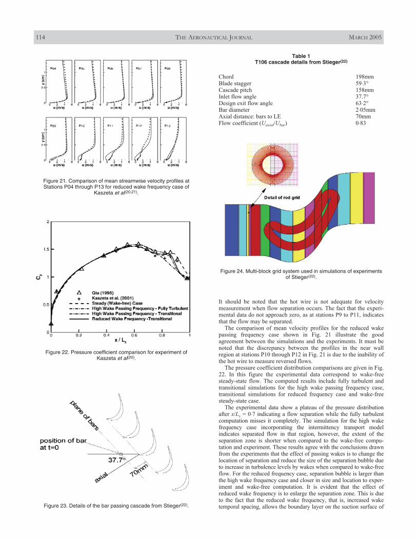
It should be noted that the hot wire is not adequate for velocitymeasurement when flow separation occurs. The fact that the experi-mental data do not approach zero, as at stations P9 to P11, indicatesthat the flow may be separated.

The comparison of mean velocity profiles for the reduced wakepassing frequency case shown in Fig. 21 illustrate the goodagreement between the simulations and the experiments. It must benoted that the discrepancy between the profiles in the near wallregion at stations P10 through P12 in Fig. 21 is due to the inability ofthe hot wire to measure reversed flows.

The pressure coefficient distribution comparisons are given in Fig.22. In this figure the experimental data correspond to wake-freesteady-state flow. The computed results include fully turbulent andtransitional simulations for the high wake passing frequency case,transitional simulations for reduced frequency case and wake-freesteady-state case.

The experimental data show a plateau of the pressure distributionafter x/Lx = 0⋅7 indicating a flow separation while the fully turbulentcomputation misses it completely. The simulation for the high wakefrequency case incorporating the intermittency transport modelindicates separated flow in that region, however, the extent of theseparation zone is shorter when compared to the wake-free compu-tation and experiment. These results agree with the conclusions drawnfrom the experiments that the effect of passing wakes is to change thelocation of separation and reduce the size of the separation bubble dueto increase in turbulence levels by wakes when compared to wake-freeflow. For the reduced frequency case, separation bubble is larger thanthe high wake frequency case and closer in size and location to exper-iment and wake-free computation. It is evident that the effect ofreduced wake frequency is to enlarge the separation zone. This is dueto the fact that the reduced wake frequency, that is, increased waketemporal spacing, allows the boundary layer on the suction surface of


Figure 21. Comparison of mean streamwise velocity profiles atStations P04 through P13 for reduced wake frequency case of

Kaszeta et al(20,21).

Figure 22. Pressure coefficient comparison for experiment of Kaszeta et al(20).

Figure 23. Details of the bar passing cascade from Stieger(22).

Table 1T106 cascade details from Stieger(22)

Chord 198mmBlade stagger 59⋅3°Cascade pitch 158mmInlet flow angle 37.7°Design exit flow angle 63⋅2°Bar diameter 2⋅05mmAxial distance: bars to LE 70mmFlow coefficient (Uaxial/Ubar) 0⋅83

Figure 24. Multi-block grid system used in simulations of experimentsof Stieger(22).

the blade a much longer time to recover from the perturbations of thewakes and allows the boundary layer to reach a state which is muchlike the steady flow case without the moving bars.

Overall, simulations were able to capture the flow features wellfor experiments of Kaszeta et al(20,21). The prediction capabilities ofthe intermittency transport model for simulations of unsteadywake–blade interaction flowfields are illustrated. Further details ofthese simulations can be found in Suzen and Huang(25).

3.8 Unsteady wake–blade interaction experiments of Stieger(22)

The experiments performed by Stieger(22) involve T106 turbine bladecascade subjected to wake passing from a moving bar wakegenerator. These experiments were conducted in order to investigatethe interaction of a convected wake and a separation bubble on therear suction surface of a highly loaded low-pressure turbine blade.The wakes shed from upstream blade rows in a real turbine aresimulated by an array of cylindrical bars moving across the inletplane of the cascade.

The unsteady wake-passing flow conditions were chosen to matchthose of a repeating stage of the T106 profile. The Reynolds numberbased on chord and inlet velocity was Re = 91,077 and thefreestream turbulence intensity was FSTI = 0⋅1%. The flow coeffi-cient for the cascade was φ = 0⋅83. The bar pitch matched thecascade pitch so that sb/sc = 1. The bar diameter of 2⋅05mm waschosen to match the loss of a representative turbine blade. Thecascade incidence was set to α1 = 37⋅7°. The details of the T106cascade set up are shown in Fig. 23 and are summarised in Table 1.

In the experiments, a series of boundary-layer traverses wereperformed using 2D LDA. The results obtained provided new insightinto the wake-induced transition mechanisms on low-pressureturbine blades.

Simulations of experiments of Stieger are performed using themulti-block grid system consisting of 18 zones and 0⋅8m grid pointsshown in Fig. 24. The rod grid shown in the inset and the two zonesit overlaps move with the specified bar speed of 1⋅2 times the axialflow velocity. The grid system has the first y+ less than 0⋅5 near solidwalls. The origin is located at the leading edge of the blade for thisgrid system. Periodic boundary conditions are employed at top andbottom boundaries.

Predicted instantaneous and phase averaged vorticity isocontoursare shown in Figs 25(a) and (b), respectively. In this case theReynolds number based on bar diameter and flow speed over the baris 1,650. The instantaneous vortex shedding behind the bar is sharperand the wake is narrower when compared to the phase averagedcontours. The smoothing effect of phase averaging is evident fromthe wake velocity profile shown in Fig. 26.

In Fig. 26, the predicted wake velocity profile is compared toexperiment at a location of x/C = –0⋅04 before the blade leadingedge. The phase averages of five different sets of six-cycle data isshown along with the phase average of hundred cycles. The fluctua-tions are apparent in each of the six-cycle averages. However, thesefluctuations are smoothed out as a larger number of cycles areincluded in averaging. The average of 100 cycles closely representthe wake profile observed in the experiment.


Figure 26. Comparison of computational and experimental wakevelocity profiles before the blade leading edge for experiments of

Stieger(22).

(b) Phase averaged(a) Instantaneous

Figure 25. Computed vorticity contours for experiment of Stieger(22).

The predicted time average pressure coefficient distributioncompares well with the experiment as shown in Fig. 27. In thisfigure the steady state experiment without the moving bars is alsoincluded in order to illustrate the effect of wake interaction on thesuction side pressure distribution. In the steady state case, there is alarge separation bubble on the suction side of the blade characterisedby the plateau in the pressure coefficient distribution between s/so =0⋅7 and 0⋅83. On the other hand, time average Cp distributionobtained from the case with moving bars does not exhibit such aplateau, indicating attached mean flow over the suction surface. Thisis due to the effect of the wakes interacting with the boundary layeron the suction surface causing transition to turbulence and hencereducing the susceptibility of the flow to separate.

Comparisons between the computed and experimental phase-averaged streamwise velocity variations at nine stations on thesuction side of the blade are shown in Figs 28(a) through 28(i). Inthese figures, the horizontal axis corresponds to the phase angle indegrees and the vertical axis correspond to the distance normal to thewall nondimensionalised by chord. The numerical results are in goodagreement with the experiment. The movement of the wake inter-action region characterised by the maximum velocity is capturedwell in the simulations.

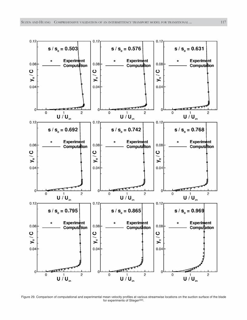
The predicted mean velocity profiles at nine stations along thesuction surface are compared to experiment in Fig. 29. The simula-tions agree very well with the experimental data.

The good agreement obtained between the simulations and theexperimental data illustrate the predicting capabilities and versatilityof the transition model in predicting unsteady wake–blade inter-action flowfields.

4.0 CONCLUDING REMARKSA transport equation for the intermittency factor is employed topredict a wide range of low-pressure turbine experiments repre-senting the effects of diverse flow conditions on transition includingthe effects of pressure gradients, freestream turbulence intensities,Reynolds number variations, flow separation/reattachment, andunsteady wake–blade interactions. The intermittent behaviour of thetransitional flows is taken into account by modifying the eddyviscosity with the intermittency factor. Comparisons of thecomputed and experimental data are made and overall goodagreement with the experimental data is obtained demonstrating thepredicting capabilities of the current intermittency approach and theintermittency transport model. Although its dependence on the

boundary-layer momentum thickness and streamwise distance limitsits extension to three dimensional applications and unstructuredgrids, the success of the intermittency model and the accompanying


Figure 27. Comparison of computational and experimental pressurecoefficient distributions for experiments of Stieger(22).

Figure 28. Comparison of computed and experimental velocity distrib-utions at various streamwise station on suction surface of the blade for

experiments of Stieger(22). Horizontal axis: phase angle (0 to 360degrees). Vertical axis: wall normal distance yn/C (0 to 0⋅08). Contour

levels: –0⋅5 to 2⋅2.


Figure 29. Comparison of computational and experimental mean velocity profiles at various streamwise locations on the suction surface of the bladefor experiments of Stieger(22).

correlations in accurately predicting transitional low-pressure turbineflows under diverse conditions has proven that the intermittencytransport modelling approach provides an accurate and practicalcomputational tool for transitional flow simulations. The success ofthe model and in particular the intermittency transport modellingapproach for two dimensional flow computations has been instru-mental in development of a more advanced transition model byMenter et al(42) based on local variables which does not have thelimitations of the current model and readily applicable to threedimensional simulations and unstructured grids.

ACKNOWLEDGEMENTSThis work is supported by NASA Glenn Research Center undergrant NCC3-590 and followed by grant NCC3-1040. The project ispart of the low pressure turbine flow physics program of NASA-Glenn. We like to thank Dr David Ashpis for his coordination of theLPT effort. We would also like to thank Drs Terrence W. Simon,Richard W. Kaszeta, Ralph J. Volino, Thomas C. Corke, Flint O.Thomas, James P. Lake, and Paul I. King and Lennart S. Hultgrenfor providing their experimental data for this effort. The authors alsoappreciate Dr Howard Hodson’s suggestion of T106 cascade experi-ments as a test case.

REFERENCES1. MAYLE, R.E. The role of laminar-turbulent transition in gas turbine

engines, ASME J Turbomachinery, 1991, 113, pp 509-537.2. RIVIR, R.B. Transition on turbine blades and cascades at low Reynolds

numbers, 1996, AIAA Paper 96-2079.3. LAKE, J.P., KING, P.I. and RIVIR, R.B. Low Reynolds number loss

reduction on turbine blades with dimples and V-grooves, 2000, AIAAPaper 2000-0738.

4. SHARMA, O. Impact of Reynolds number on LP turbine performance,1998, NASA/CP-1998-206958, pp 65-70.

5. SIMON, F.F. and STEPHENS, C.A. Modeling of the heat transfer in bypasstransitional boundary-layer flows, 1991, NASA Technical Paper 3170.

6. DHAWAN, S. and NARASIMHA, R. Some properties of boundary layerduring the transition from laminar to turbulent flow motion, J FluidMechanics, 1958, 3, pp 418-436.

7. GOSTELOW, J.P., BLUNDEN, A.R. and WALKER, G.J. Effects of free-stream turbulence and adverse pressure gradients on boundary layertransition, ASME J Turbomachinery, 1994, 116, pp 392-404.

8. SOLOMON, W.J., WALKER, G.J. and GOSTELOW, J.P. Transition lengthprediction for flows with rapidly changing pressure gradients, 1995,ASME Paper ASME-95-GT-241.

9. STEELANT, J. and DICK, E. Modelling of bypass transition with condi-tioned Navier-Stokes equations coupled to an intermittency transportequation, Int J for Numerical Methods in Fluids, 1996, 23, pp 193-220.

10. CHO, J.R. and CHUNG, M.K. A k-ε-γ equation turbulence model, J FluidMechanics, 1992, 237, pp 301-322.

11. DRIKAKIS, D. and GOLDBERG, U. Wall-distance-free turbulence modelsapplied to incompressible flows, Int J Computational Fluid Dynamics,1998, 10, pp 241-253.

12. SUZEN, Y.B. and HUANG, P.G. Modelling of flow transition using anintermittency transport equation, 1999, NASA-CR-1999-209313.

13. SAVILL, A.M. Some recent progress in the turbulence modeling of by-pass transition, 1993, Near-Wall Turbulent Flows, SO, R.M.C.,SPEZIALE, C.G. and LAUNDER, B.E. (Eds), pp 829-848, Elsevier Science.

14. SAVILL, A.M. Further progress in the turbulence modeling of by-passtransition, 1993, Engineering Turbulence Modeling and Experiments 2,RODI, W. and MARTELLI, F. (Eds), pp 583-592, Elsevier Science.

15. SIMON, T.W., QIU, S. and YUAN, K. Measurements in a transitionalboundary layer under low-pressure turbine airfoil conditions, 2000,NASA-CR-2000-209957.

16. VOLINO, R.J. and HULTGREN, L.S. Measurements in separated andtransitional boundary layers under low-pressure turbine airfoil condi-tions, 2000, ASME/IGTI Paper 2000-GT-0260.

17. LAKE, J.P., KING, P.I. and RIVIR, R.B. Reduction of separation losses ona turbine blade with low Reynolds number, 1999, AIAA Paper AIAA-99-0242.

18. HUANG, J., CORKE, T.C. and THOMAS, F.O. Plasma actuators forseparation control of low pressure turbine blades, 2003, AIAA PaperNo AIAA-2003-1027.

19. VOLINO, R.J. Separated flow transition under simulated low-pressureturbine airfoil conditions: Part 1- Mean flow and turbulence statistics,2002, ASME Paper ASME-GT-30236.

20. KASZETA, R.W., SIMON, T.W. and ASHPIS, D.E. Experimental investi-gation of transition to turbulence as affected by passing wakes, 2001,ASME Paper 2001-GT-0195.

21. KASZETA, R.W., SIMON, T.W., OTTAVIANI, F. and JIANG, N. Theinfluence of wake passing frequency and elevated free stream turbu-lence intensity on transition in low-pressure turbines, 2003, AIAAPaper AIAA-2003-3633.

22. STIEGER, R.D. The Effects of Wakes on Separating Boundary Layers inLow-pressure Turbines, 2002, PhD dissertation, Cambridge University,Engineering Department.

23. SUZEN, Y.B. and HUANG, P.G. Modeling of flow transition using anintermittency transport equation, 2000, AIAA Paper AIAA-2000-0287.

24. SUZEN, Y.B. and HUANG, P.G. Modeling of flow transition using anintermittency transport equation, J Fluids Eng, 2000, 122, pp 273-284.

25. SUZEN, Y.B. and HUANG, P.G. Numerical simulation of transitionalflows as affected by passing wakes, 2004, AIAA Paper AIAA-2004-0103.

26. SUZEN, Y.B., XIONG, G. and HUANG, P.G. Predictions of transitionalflows in low-pressure turbines using an intermittency transportequation, 2000, AIAA Paper AIAA-2000-2654.

27. SUZEN, Y.B. and HUANG, P.G., HULTGREN, L.S., ASHPIS, D.E.Predictions of separated and transitional boundary layers under low-pressure turbine airfoil conditions using an intermittency transportequation, 2001, AIAA Paper AIAA-2001-0446.

28. SUZEN, Y.B., XIONG, G. and HUANG, P.G. Predictions of transitionalflows in low-pressure turbines using an intermittency transportequation, AIAA J, 2002, 40, (2), pp 254-266.

29. SUZEN, Y.B., HUANG, P.G., HULTGREN, L.S. and ASHPIS, D.E.Predictions of separated and transitional boundary layers under low-pressure turbine airfoil conditions using an intermittency transportequation, ASME J Turbomachinery, 2003, 125, pp 455-464.

30. SUZEN, Y.B., HUANG, P.G., VOLINO, R.J., CORKE, T.C., THOMAS, F.O.,HUANG, J., LAKE, J.P. and KING, P.I. A comprehensive CFD study oftransitional flows in low-pressure turbines under a wide range ofoperating conditions, 2003, AIAA Paper AIAA-2003-3591.

31. MENTER, F.R. Two-equation eddy-viscosity turbulence models forengineering applications, AIAA J, 1994, 32, (8), pp 1598-1605.

32. ABU-GHANNAM, B.J. and SHAW, R. Natural transition of boundarylayers-The effects of turbulence, pressure gradient, and flow history, JMech Eng Sci, 1980, 22, (5), pp 213-228.

33. DAVIS, R.L., CARTER, J.E. and RESHOTKO, E. Analysis of transitionalseparation bubbles on infinite swept wings, AIAA J, 1987, 25, (3), pp421-428.

34. HUANG, P.G. and COAKLEY, T.J. An implicit Navier-Stokes code forturbulent flow modeling, 1992, AIAA Paper AIAA-92-0547.

35. RHIE, C.M. and CHOW, W.L. Numerical study of the turbulent flow pastan airfoil with trailing edge separation, AIAA J, 1983, 21, pp 1525-1532.

36. LAUNDER, B.E. and SHARMA, B.I. Application of the energy dissipationmodel of turbulence to the calculation of flow near a spinning disc,Letters in Heat and Mass Transfer, 1974, 1, pp 131-138.

37. HSU, M.C., VOGIATZIS, K. and HUANG, P.G. Validation and implemen-tation of advanced turbulence models in swirling and separated flows,2003, AIAA Paper AIAA 2003-0766.

38. QUI, S. and SIMON, T.W. An experimental investigation of transition asapplied to low pressure turbine suction surface flows, 1997, ASMEPaper 97-GT-455.

39. JIANG, N. and SIMON, T.W. The influence of unsteady acceleration andturbulence intensity on transition in low-pressure turbines, 2003, AIAAPaper AIAA-2003-3630.

40. JIANG, N. and SIMON, T.W. Modeling laminar-to-turbulent transition ina low-pressure turbine flow which is unsteady due to passing wakes:Part I, Transition onset, 2003, ASME Paper ASME-GT2003-38787.

41. JIANG, N. and SIMON, T.W. Modeling laminar-to-turbulent transition ina low-pressure turbine flow which is unsteady due to passing wakes:Part II, Transition path, 2003, ASME Paper ASME-GT2003-38963.

42. MENTER, F.R., LANGTRY, R.B., LIKKI, S.R., SUZEN, Y.B., HUANG, P.G.and VOELKER, S. A correlation based transition model using localvariables Part I — Model formulation, 2004, ASME Paper ASME-GT2004-53452.


comprehensive validation of an intermittency transport … · · 2011-08-10the boundary layer...

Documents