comprehensive two-dimensional gas chromatography ... · university of helsinki department of...

University of Helsinki

Department of Chemistry

Laboratory of Analytical Chemistry

Finland

Comprehensive Two-Dimensional Gas Chromatography:

Instrumental and Methodological Development

Minna Katriina Kallio

Academic Dissertation

To be presented with the permission of the Faculty of Science of the University ofHelsinki for public criticism in Auditorium A 129 of the Kumpula Chemistry Building

April 25, 2008, at 12 o´clock noon.

Helsinki 2008

2

Custos:

Prof. Tuulia HyötyläinenLaboratory of Analytical Chemistry

Department of ChemistryUniversity of Helsinki

Finland

Reviewers:Prof. Hans-Gerd Janssen

Central Analytical ScienceUnilever Research and Development

The Netherlandsand

Dr. Erkki SippolaForensic Laboratory

National Bureau of InvestigationFinland

Opponent:

Prof. Peter J. SchoenmakersVan ‘t Hoff Institute for Molecular Sciences

University of AmsterdamThe Netherlands

ISBN 978-952-92-3717-3 (paperback)

ISBN 978-952-10-4645-2 (PDF)

http://ethesis.helsinki.fi

Yliopistopaino, Helsinki 2008

http://ethesis.helsinki.fi

3

CONTENT

PREFACE .................................................................................................................. 5

ABSTRACT ............................................................................................................... 6

ABBREVIATIONS .................................................................................................... 8

LIST OF ORIGINAL PAPERS............................................................................... 10

1 INTRODUCTION AND AIMS ............................................................................ 12

2 COMPREHENSIVE TWO-DIMENSIONAL GAS CHROMATOGRAPHY.... 152.1 Operational principle ..................................................................................... 152.2 Main features.................................................................................................. 17

2.2.1 Comprehensiveness ................................................................................... 172.2.2 Orthogonality ............................................................................................ 172.2.3 Enhanced separation efficiency through increased peak capacity ............... 192.2.4 Structured chromatograms ......................................................................... 222.2.5 Capability to detect low quantities ............................................................. 23

2.3 Instrumentation and data analysis ................................................................ 242.3.1 Modulators ................................................................................................ 24

2.3.1.1 Thermal modulators ............................................................................ 242.3.1.2 Valve modulators................................................................................ 27

2.3.2 Analytical conditions ................................................................................. 282.3.2.1 Columns ............................................................................................. 282.3.2.2 Oven temperature ramp and carrier gas flow ....................................... 292.3.2.3 Detection ............................................................................................ 30

2.3.3 Data analysis ............................................................................................. 312.3.3.1 Visualisation ....................................................................................... 312.3.3.2 Comparative analysis .......................................................................... 312.3.3.3 Qualitative analysis ............................................................................. 322.3.3.4 Quantitative analysis ........................................................................... 33

2.4 Applications .................................................................................................... 36

3 EXPERIMENTAL ................................................................................................ 393.1 Chemicals and samples................................................................................... 393.2 Devices and columns....................................................................................... 393.3 Data analysis................................................................................................... 443.4 Sample preparation ........................................................................................ 45

3.4.1 Soxhlet extraction ...................................................................................... 453.4.2 Static and dynamic sonication assisted extraction....................................... 453.4.3 Sample clean-up procedures ...................................................................... 46

4

4 RESULTS AND DISCUSSION ............................................................................ 484.1 Instrumental development ............................................................................. 48

4.1.1 Development of the semi-rotating cryogenic modulator ............................. 484.1.1.1 Structure and performance of the modulators ...................................... 514.1.1.2 Comparison of modulators .................................................................. 55

4.1.2 Development of data analysis programs..................................................... 574.1.2.1 Basic operations.................................................................................. 584.1.2.2 Comparison operations........................................................................ 594.1.2.3 Identification....................................................................................... 60

4.2 Methodological development ......................................................................... 614.2.1 Sample preparation .................................................................................... 61

4.2.1.1 Dynamic sonication-assisted extraction............................................... 614.2.1.2 Sample clean-up.................................................................................. 62

4.2.2 Analytical conditions ................................................................................. 654.2.2.1 Columns ............................................................................................. 654.2.2.2 Oven temperature ramp and carrier gas flow ....................................... 684.2.2.3 Detection ............................................................................................ 69

4.2.3 Qualitative analysis.................................................................................... 694.2.3.1 Identification of target analytes ........................................................... 714.2.3.2 Identification of unkowns.................................................................... 73

4.2.4 Quantitative analysis.................................................................................. 764.2.4.1 Calibration procedures ........................................................................ 764.2.4.2 Effect of matrix on the separation........................................................ 784.2.4.3 Simplified calibration procedure ......................................................... 81

5 CONCLUSIONS ................................................................................................... 83

6 REFERENCES...................................................................................................... 85

APPENDICES: CORRECTIONS TO THE ORIGINAL PAPERSPAPERS I-IX

5

PREFACE

This thesis is based on experimental work carried out in the Laboratory of AnalyticalChemistry of the Department of Chemistry, University of Helsinki, and in theDepartment of Analytical Chemistry and Applied Spectroscopy of the Division ofChemistry, Free University, Amsterdam, during the years 2002-2008. Funding for thework was provided by the Academy of Finland, the Maj and Tor Nessling Foundation,the Alfred Kordelin Foundation and the University of Helsinki.

Sincere thanks are expressed to Prof. Marja-Liisa Riekkola and Dr. René Vreuls forgiving me the opportunity to carry out this work in their respective laboratories.

I am most grateful to my supervisor, Prof. Tuulia Hyötyläinen, for her encouragement,patience, fresh ideas and unwavering positive attitude. I am also indebted to ourlaboratory engineer, Matti Jussila, who always found time to invest in the research andin discussion, particularly as related to modulators. Special thanks are expressed toSami Palonen, Vesa Palonen and Sami Varjo for putting much effort into the programdevelopment and to Pekka Tarkiainen for his technical assistance in the construction ofthe modulators. Pentti Jyske is sincerely thank for solving a diversity of (research)problems encountered over the years.

I would like to thank former and present personnel of the laboratory for creating astimulating working atmosphere and for organising so many enjoyable and relaxingleisure-time activities. Merit Hortling is thanked for ensuring that the paper work wasdone on time and Liisa Heino for providing the chemicals, glassware and suppliesneeded in the research. Päivi Raimi and Sari Järvimäki are thanked for their assistancein the laboratory.

I am indebted to Kathleen Ahonen for improving the language of the dissertation andmost of the original papers. Prof. Hans-Gerd Janssen and Dr. Erkki Sippola are thankedfor their valuable comments on the manuscipt.

Finally, and above all, loving thanks to my caring parents Maija-Leena and Matti andmy brother Antti for their support.

6

ABSTRACT

Comprehensive two-dimensional gas chromatography (GC×GC) offers enhancedseparation efficiency, reliability in qualitative and quantitative analysis, capability todetect low quantities, and information on the whole sample and its components. Thesefeatures are essential in the analysis of complex samples, in which the number ofcompounds may be large or the analytes of interest are present at trace level. This studyinvolved the development of instrumentation, data analysis programs andmethodologies for GC×GC and their application in studies on qualitative andquantitative aspects of GC×GC analysis. Environmental samples were used as modelsamples.

Instrumental development comprised the construction of three versions of a semi-rotating cryogenic modulator in which modulation was based on two-step cryogenictrapping with continuously flowing carbon dioxide as coolant. Two-step trapping wasachieved by rotating the nozzle spraying the carbon dioxide with a motor. The fastestrotation and highest modulation frequency were achieved with a permanent magneticmotor, and modulation was most accurate when the motor was controlled with amicrocontroller containing a quartz crystal. Heated wire resistors were unnecessary forthe desorption step when liquid carbon dioxide was used as coolant. With use of themodulators developed in this study, the narrowest peaks were 75 ms at base.

Three data analysis programs were developed allowing basic, comparison andidentification operations. Basic operations enabled the visualisation of two-dimensionalplots and the determination of retention times, peak heights and volumes. Theoverlaying feature in the comparison program allowed easy comparison of 2D plots. Anautomated identification procedure based on mass spectra and retention parametersallowed the qualitative analysis of data obtained by GC×GC and time-of-flight massspectrometry.

In the methodological development, sample preparation (extraction and clean-up) andGC×GC methods were developed for the analysis of atmospheric aerosol and sedimentsamples. Dynamic sonication assisted extraction was well suited for atmosphericaerosols collected on a filter. A clean-up procedure utilising normal phase liquid

7

chromatography with ultra violet detection worked well in the removal of aliphatichydrocarbons from a sediment extract.

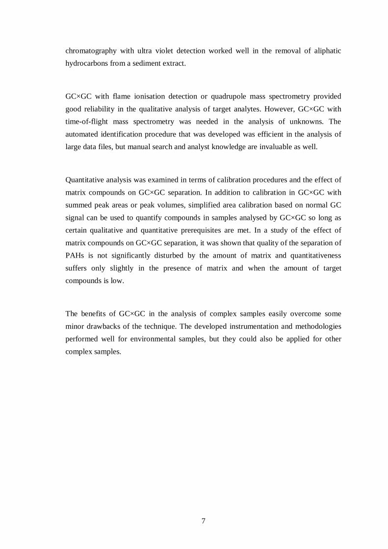
GC×GC with flame ionisation detection or quadrupole mass spectrometry providedgood reliability in the qualitative analysis of target analytes. However, GC×GC withtime-of-flight mass spectrometry was needed in the analysis of unknowns. Theautomated identification procedure that was developed was efficient in the analysis oflarge data files, but manual search and analyst knowledge are invaluable as well.

Quantitative analysis was examined in terms of calibration procedures and the effect ofmatrix compounds on GC×GC separation. In addition to calibration in GC×GC withsummed peak areas or peak volumes, simplified area calibration based on normal GCsignal can be used to quantify compounds in samples analysed by GC×GC so long ascertain qualitative and quantitative prerequisites are met. In a study of the effect ofmatrix compounds on GC×GC separation, it was shown that quality of the separation ofPAHs is not significantly disturbed by the amount of matrix and quantitativenesssuffers only slightly in the presence of matrix and when the amount of targetcompounds is low.

The benefits of GC×GC in the analysis of complex samples easily overcome someminor drawbacks of the technique. The developed instrumentation and methodologiesperformed well for environmental samples, but they could also be applied for othercomplex samples.

8

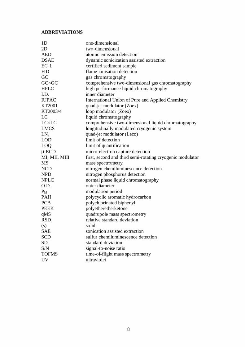
ABBREVIATIONS

1D one-dimensional2D two-dimensionalAED atomic emission detectionDSAE dynamic sonicication assisted extractionEC-1 certified sediment sampleFID flame ionisation detectionGC gas chromatographyGC×GC comprehensive two-dimensional gas chromatographyHPLC high performance liquid chromatographyI.D. inner diameterIUPAC International Union of Pure and Applied ChemistryKT2001 quad-jet modulator (Zoex)KT2003/4 loop modulator (Zoex)LC liquid chromatographyLC×LC comprehensive two-dimensional liquid chromatographyLMCS longitudinally modulated cryogenic systemLN2 quad-jet modulator (Leco)LOD limit of detectionLOQ limit of quantificationµ-ECD micro-electron capture detectionMI, MII, MIII first, second and third semi-rotating cryogenic modulatorMS mass spectrometryNCD nitrogen chemiluminescence detectionNPD nitrogen phosphorus detectionNPLC normal phase liquid chromatographyO.D. outer diameterPM modulation periodPAH polycyclic aromatic hydrocarbonPCB polychlorinated biphenylPEEK polyetheretherketoneqMS quadrupole mass spectrometryRSD relative standard deviation(s) solidSAE sonication assisted extractionSCD sulfur chemiluminescence detectionSD standard deviationS/N signal-to-noise ratioTOFMS time-of-flight mass spectrometryUV ultraviolet

9

SYMBOLS

∅ diameterα saturation factorσ standard deviation of a Gaussian peak [s]

∞si,γ activity coefficient of compound i at infinite dilution in

stationary phaseH plate height [m]I linear retention indexIexp experimental linear retention indexIlit linear retention index reported in literatureki retention factor of compound iL length of column [m]m approximation for number of single component peaksn number of separation stages in any separation systemnc peak capacityN plate numberp number of peaks

0ip vapour pressure of pure substance i [Pa]

s number of singlets; dimensionality of a sampleTe temperature at the time of elution [K]tR retention time [s]1tR 1st-dimension retention time2tR 2nd-dimension retention timetmin retention time of the first component [s]tmax retention time of the last component [s]

10

LIST OF ORIGINAL PAPERS

This thesis is based on the following nine papers, hereafter referred to by their Romannumerals [I-IX]

I Hyötyläinen T, Kallio M, Hartonen K, Jussila M, Palonen S, Riekkola M-L,2002, Anal. Chem. 74: 4441-4446, Modulator Design for Comprehensive Two-Dimensional Gas Chromatography: Quantitative Analysis of PolyaromaticHydrocarbons and Polychlorinated Biphenyls. Copyright 2002 American Chemical

Society

II Kallio M, Hyötyläinen T, Jussila M, Hartonen K, Palonen S, Riekkola M-L,2003, Anal. Bioanal. Chem. 375: 725-731, Semi-Rotating CryogenicModulator for Comprehensive Two-Dimensional Gas Chromatography.Copyright 2003 Springer-Verlag

III Kristenson ME, Korytar P, Danielsson C, Kallio M, Brandt M, Mäkelä J, VreulsRJJ, Beens J, Brinkman UAth, 2003, J. Chromatogr. A 1019: 65-77, Evaluationof Modulators and Electron-Capture Detectors for Comprehensive Two-Dimensional GC of Halogenated Organic Compounds. Copyright 2003 Elsevier

Science

IV Kallio M, Hyötyläinen T, Lehtonen M, Jussila M, Hartonen K, Shimmo M,Riekkola M-L, 2003, J. Chromatogr. A 1019: 251-260, Comprehensive Two-Dimensional Gas Chromatography in the Analysis of Urban Aerosols. Copyright

2003 Elsevier Science

V Kallio M, Jussila M, Rissanen T, Anttila P, Hartonen K, Reissell A, Vreuls RJJ,Adahchour M, Hyötyläinen T, 2006, J. Chromatogr. A 1125: 234-243,Comprehensive Two-Dimensional Gas Chromatography Coupled to Time-of-Flight Mass Spectrometry (GC×GC-TOFMS) in the Identification of OrganicCompounds in Atmospheric Aerosols from Coniferous Forest. Copyright 2006

Elsevier Science

11

VI Kallio M, Hyötyläinen T, 2007, J. Chromatogr. A 1148: 228–235, QuantitativeAspects in Comprehensive Two-Dimensional Gas Chromatography. Copyright

2007 Elsevier Science

VII Kallio M, Hyötyläinen T, accepted for publication in J. Chromatogr. A, SimpleCalibration Procedure for Comprehensive Two-Dimensional GasChromatography.

VIII Kallio M, Jussila M, Raimi P, Hyötyläinen T, accepted for publication in Anal.Bioanal. Chem. Modified Semi-Rotating Cryogenic Modulator forComprehensive Two-Dimenisonal Gas Chromatography.

IX Kallio M, Varjo S, Jussila M, Kivilompolo M, Järvimäki S, Hyötyläinen T,manuscript, submitted to Analyst, Data Analysis Programs for ComprehensiveTwo-Dimenisonal Chromatography.

I took the main responsibility for the experimental work, data evaluation and writing ofpapers II, IV-IX. In paper I I was responsible for the experimental work and in paperIII for the experimental work and for writing the part of the paper related to the testingof the semi-rotating cryogenic modulator.

12

1 INTRODUCTION AND AIMS

Analysis of complex samples is challenging when the number of compounds is large orthe analytes are present at just trace level. Traditional one-dimensionalchromatographic techniques, such as gas chromatography, often fail to separatecompounds well enough, and severe overlap of peaks results. Reliable identificationand quantification are then hindered. Multidimensional techniques, in which samplecomponents are subjected to at least two different separation steps, offer enhancedefficiency by providing more space for the separation. Component peaks can spread outacross additional coordinates, and peak overlap is reduced [Giddings 1995]. Inconventional multidimensional techniques only one or a few fractions are transferredfrom the first to the second dimension, but in comprehensive two-dimensionaltechniques the whole sample passes through the whole system, and information isobtained on the total sample.

Comprehensive two-dimensional gas chromatography (GC×GC), an increasinglypopular multidimensional technique, was introduced in 1991 [Liu and Phillips 1991].At the end of the 1990s and the beginning of the 21st century, the major effort was putinto the development of modulators. Most of the early applications were targeted at theanalysis of petrochemical products, to the extent that many mistakenly thought thatGC×GC was only suitable for oil analysis. During the last five to six years the numberof GC×GC publications has risen to nearly 350 and the range of applications haswidened dramatically. Besides petrochemical analysis, GC×GC is nowadays used in theanalysis of food, environmental, biological, essential oil and cosmetic samples. Thegreat and growing popularity of the technique rests on the availability of commercialinstruments and software, but most of all on greater awareness of the many advantagesof the technique.

The aim of this study was to construct new instrumentation and software for GC×GCand to demonstrate its performance in qualitative and quantitative analysis of highlycomplex environmental samples. Since no commercial cryogenic modulators wereavailable in the year 2000 when the GC×GC project was initiated at the University ofHelsinki, the first challenge was to construct a rugged and reliable modulator [I].Thereafter two modifications of the modulator were built with a view to improving theperformance [II, VIII]. The second modification was evaluated in a comparison with

13

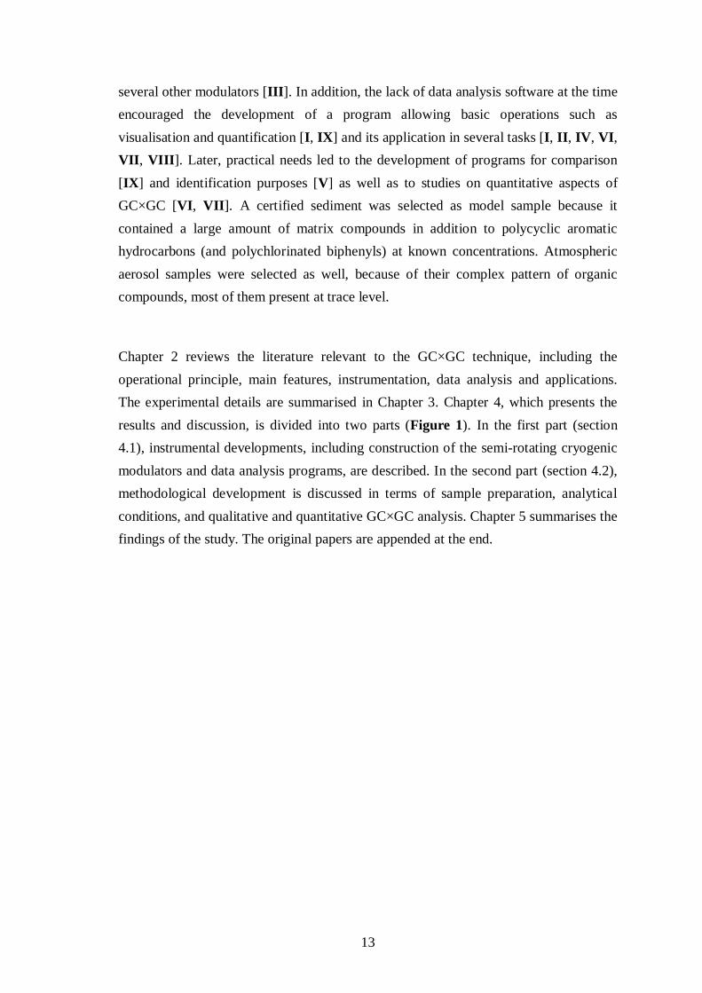
several other modulators [III]. In addition, the lack of data analysis software at the timeencouraged the development of a program allowing basic operations such asvisualisation and quantification [I, IX] and its application in several tasks [I, II, IV, VI,VII, VIII]. Later, practical needs led to the development of programs for comparison[IX] and identification purposes [V] as well as to studies on quantitative aspects ofGC×GC [VI, VII]. A certified sediment was selected as model sample because itcontained a large amount of matrix compounds in addition to polycyclic aromatichydrocarbons (and polychlorinated biphenyls) at known concentrations. Atmosphericaerosol samples were selected as well, because of their complex pattern of organiccompounds, most of them present at trace level.

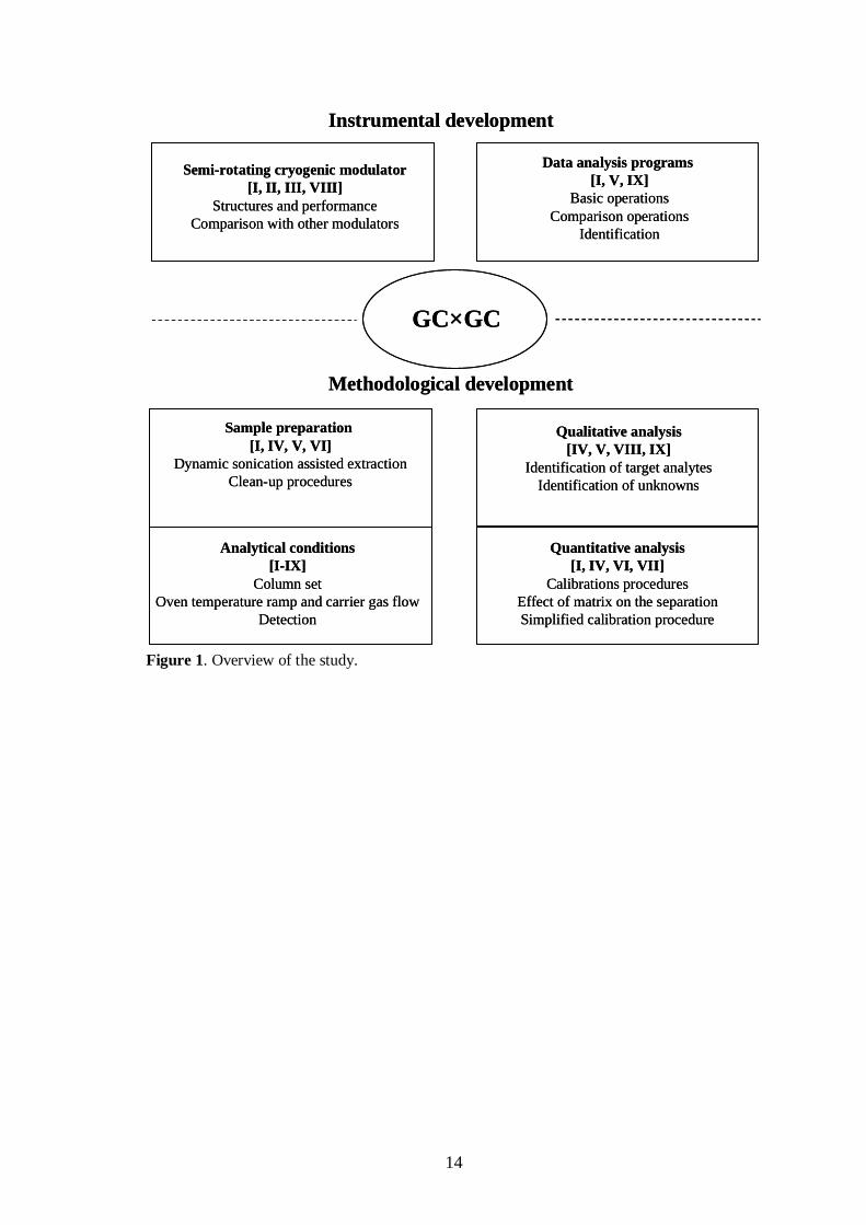
Chapter 2 reviews the literature relevant to the GC×GC technique, including theoperational principle, main features, instrumentation, data analysis and applications.The experimental details are summarised in Chapter 3. Chapter 4, which presents theresults and discussion, is divided into two parts (Figure 1). In the first part (section4.1), instrumental developments, including construction of the semi-rotating cryogenicmodulators and data analysis programs, are described. In the second part (section 4.2),methodological development is discussed in terms of sample preparation, analyticalconditions, and qualitative and quantitative GC×GC analysis. Chapter 5 summarises thefindings of the study. The original papers are appended at the end.

14

Figure 1. Overview of the study.

GC×GC

Semi-rotating cryogenic modulator[I, II, III, VIII]

Structures and performanceComparison with other modulators

Qualitative analysis[IV, V, VIII, IX]

Identification of target analytesIdentification of unknowns

Data analysis programs[I, V, IX]

Basic operationsComparison operations

Identification

Quantitative analysis[I, IV, VI, VII]

Calibrations proceduresEffect of matrix on the separationSimplified calibration procedure

Instrumental development

Sample preparation[I, IV, V, VI]

Dynamic sonication assisted extractionClean-up procedures

Methodological development

Analytical conditions[I-IX]

Column setOven temperature ramp and carrier gas flow

Detection

GC×GC

Semi-rotating cryogenic modulator[I, II, III, VIII]

Structures and performanceComparison with other modulators

Qualitative analysis[IV, V, VIII, IX]

Identification of target analytesIdentification of unknowns

Data analysis programs[I, V, IX]

Basic operationsComparison operations

Identification

Quantitative analysis[I, IV, VI, VII]

Calibrations proceduresEffect of matrix on the separationSimplified calibration procedure

Instrumental development

Sample preparation[I, IV, V, VI]

Dynamic sonication assisted extractionClean-up procedures

Methodological development

Analytical conditions[I-IX]

Column setOven temperature ramp and carrier gas flow

Detection

15

2 COMPREHENSIVE TWO-DIMENSIONAL GAS CHROMATOGRAPHY

2.1 Operational principle

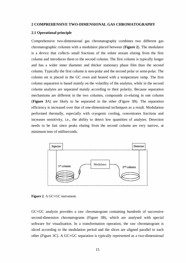
Comprehensive two-dimensional gas chromatography combines two different gaschromatographic columns with a modulator placed between (Figure 2). The modulatoris a device that collects small fractions of the solute stream eluting from the firstcolumn and introduces them to the second column. The first column is typically longerand has a wider inner diameter and thicker stationary phase film than the secondcolumn. Typically the first column is non-polar and the second polar or semi-polar. Thecolumn set is placed in the GC oven and heated with a temperature ramp. The firstcolumn separation is based mainly on the volatility of the analytes, while in the secondcolumn analytes are separated mainly according to their polarity. Because separationmechanisms are different in the two columns, compounds co-eluting in one column(Figure 3A) are likely to be separated in the other (Figure 3B). The separationefficiency is increased over that of one-dimensional techniques as a result. Modulationperformed thermally, especially with cryogenic cooling, concentrates fractions andincreases sensitivity, i.e., the ability to detect low quantities of analytes. Detectionneeds to be fast since peaks eluting from the second column are very narrow, atminimum tens of milliseconds.

Figure 2. A GC×GC instrument.

GC×GC analysis provides a raw chromatogram containing hundreds of successivesecond-dimension chromatograms (Figure 3B), which are analysed with specialsoftware for visualisation. In a transformation operation, the raw chromatogram issliced according to the modulation period and the slices are aligned parallel to eachother (Figure 3C). A GC×GC separation is typically represented as a two-dimensional

1st column 2nd column

Injector Detector

Modulator1st column 2nd column

Injector Detector

Modulator

16

plot (Figure 3D), in which the x-axis represents the retention in the first column and they-axis the retention in the second column. Height of the peak is indicated with contoursor colour scale. In a three-dimensional representation (Figure 3E), the z-axis indicatesthe detection response.

Figure 3. Visualisation of GC×GC separation. (A) separation at the end of the first column, (B)separation at the detector, i.e., at the end of the second column, (C) sliced raw chromatogram,(D) 2D plot and (E) 3D plot.

First dimensionSecond dimension

Seco

nddi

men

sion

First dimension

Raw chromatogramat the end of the second column

At the end of the first column

First dimension Seco

nddi

men

sion

2D plot

3D plot

A

B

C

D

E

Det

ecto

rres

pons

e

First dimensionSecond dimension

Seco

nddi

men

sion

First dimension

Raw chromatogramat the end of the second column

At the end of the first column

First dimension Seco

nddi

men

sion

2D plot

3D plot

A

B

C

D

E

Det

ecto

rres

pons

e

17

2.2 Main features

The main features of GC×GC, including comprehensiveness, orthogonality, peakcapacity, structured chromatograms and capability to detect low quantities, areintroduced below.

2.2.1 Comprehensiveness

In contrast to conventional multidimensional chromatography in which only one or a

few fractions are transferred from the first to the second column, in GC×GC the whole

sample is subjected to the second-column separation. This provides comprehensiveinformation on the entire sample and its components. Schoenmakers et al. [2003] haveproposed the following criteria for a two-dimensional separation that is comprehensive:

1. Every part of the sample is subjected to two different separations.

2. Equal percentages of all sample components pass through the two columns andeventually reach the detector.

3. The separation obtained in the first dimension is essentially maintained.

The first and third criteria were already proposed by Giddings [1987] formultidimensional separations. The second criterion indicates that if mass transfer fromthe first to the second column is less than 100%, the chromatogram obtained has to beidentical to that which corresponds to 100% mass transfer.

2.2.2 Orthogonality

The term orthogonal is well defined in mathematics and statistics where it is related toperpendicularity of vectors or functions, or to the independence of variables[Schoenmakers et al. 2003]. The term is less well defined in separation science, but isconsidered to describe a situation, in which two separation mechanisms differ fromeach other. In 2D chromatography it implies that completely different retentionmechanisms apply in the two dimensions. Orthogonality is closely related to peakcapacity (see section 2.2.3).

Two approaches have been developed to evaluate the orthogonality in GC×GCmathematically, i.e., to obtain a numerical measure for it. In the approach of Liu andPatterson Jr. [1995], solute retention parameters and factor analysis were used to define

18

a peak spreading angle and correlation, from which a practical peak capacity was

calculated. A spreading angle of 90° represents the theoretical maximum of peak

capacity. While the method can be applied to a specific sample, it does not give auniversal measure of orthogonality. In the more recent approach of Ryan et al. [2005a],the polarity of the column set was varied and othogonality was calculated as thedifference in the amounts of the separation space defined by the least-to-most retainedsolutes relative to the void time. Because the measure of the orthogonality is a ratio,different column sets can be directly compared regardless of the modulation period.

Instead of evaluating orthogonality mathematically, Venkatramani et al. [1996]demonstrated it experimentally by comparing isothermal and temperature gradientanalyses in the first and second dimensions. They concluded that when a temperaturegradient is used in both dimensions, the GC×GC separation is properly tuned, retentiontimes in the two dimensions are independent of each other, and the two-dimensionalchromatogram is orthogonal. Independence of the separation was demonstrated aconstant second-dimension retention within a homologous series. Recently, it has beenshown that similar results as those of Venkatramani et al. can be obtained even thoughthe second dimension separation takes place under isothermal conditions.

Yet a third way to investigate orthogonality is in terms of retention factor. According tothe definition of the International Union of Pure and Applied Chemistry (IUPAC), theretention factor is a measure of the time the sample component resides in the stationaryphase relative to the time it resides in the mobile phase. For compound i, retentionfactor ki is inversely proportional to the activity coefficient at infinite dilution in the

stationary phase, ∞si,γ , and the vapour pressure of the pure substance, 0

ip , according to

equation (1) [Beens et al. 1998a; Schoenmakers et al. 2000].

0,

1

isii p

k⋅

≅ ∞γ(1)

Volatility is the prevailing separation mechanism in the first dimension of GC×GC.Vapour pressure is related to the boiling point of the compound, and each solute has itsown pressure versus temperature relationship. When linear temperature programming is

applied, vapour pressures of the compounds at the time of elution 0ip (Te) are

approximately equal. Because the separation in the second dimension is fast, it can be

19

considered isothermal at the temperature of elution Te. Hence, vapour pressure does notplay a role in the second dimension, but the separation is influenced only by the activitycoefficient, i.e., polar interactions.

2.2.3 Enhanced separation efficiency through increased peak capacity

Peak capacity is the term used to describe separation efficiency. It is defined as themaximum number of peaks that can fit into an available separation space at a givenresolution. Peak capacity, nc, can be calculated with equation (2), where N is platenumber, tmin the retention time of the first component and tmax the retention time of thelast component.

)ln(4

1min

max2/1

ttNnc += (2)

According to equation (2), peak capacity is proportional to the square root of platenumber N. The plate number, in turn, is proportional to the length of the column, L, andinversely proportional to the plate height, H, as presented in equation (3).

HLN = (3)

Plate height is related to the column length, the standard deviation, σ, and the retentiontime, tR, of the Gaussian peak according to equation (4).

2

2

RtLH σ

= (4)

Plate number can be increased (i) by increase in the column length or (i) by decrease inthe plate height. Since increasing the column length is not an attractive option, the moreeffective approach is to decrease the plate height by reducing the inner diameter of thecolumn. The growth of the plate number is slow, however: to achieve 10-fold increasein peak capacity would require 100-fold increase in plate number. A more effectiveway to increase peak capacity is to use a multidimensional separation system.

The peak capacity plays an essential role in the statistical theory of overlap, which isused to describe the 1D and 2D separations. Statistically the chromatographicseparation process is a deterministic phenomenon: it can be predicted from chemicaland physical properties [Davis and Samuel 2000]. Sometimes, however, the complexity

20

of a mixture is so great that the deterministic information is neither available norattainable [Davis 1997] and the frequency of overlap can be described with probabilitytheory. The statistical theory of overlap assumes that components are randomlydistributed into the separation space. The number of peaks varies from separation toseparation and it is impossible that all separations will contain the same numbers of

peaks. The statistical approximation for the number of peaks in any separation is m .

The saturation factor, α, is a measure of overlap and it is defined as the average number

of components, m , divided by the peak capacity [Shi and Davis 1993], according to

equation 5. If α is large, the number of overlapping components is large.

α =mnc

(5)

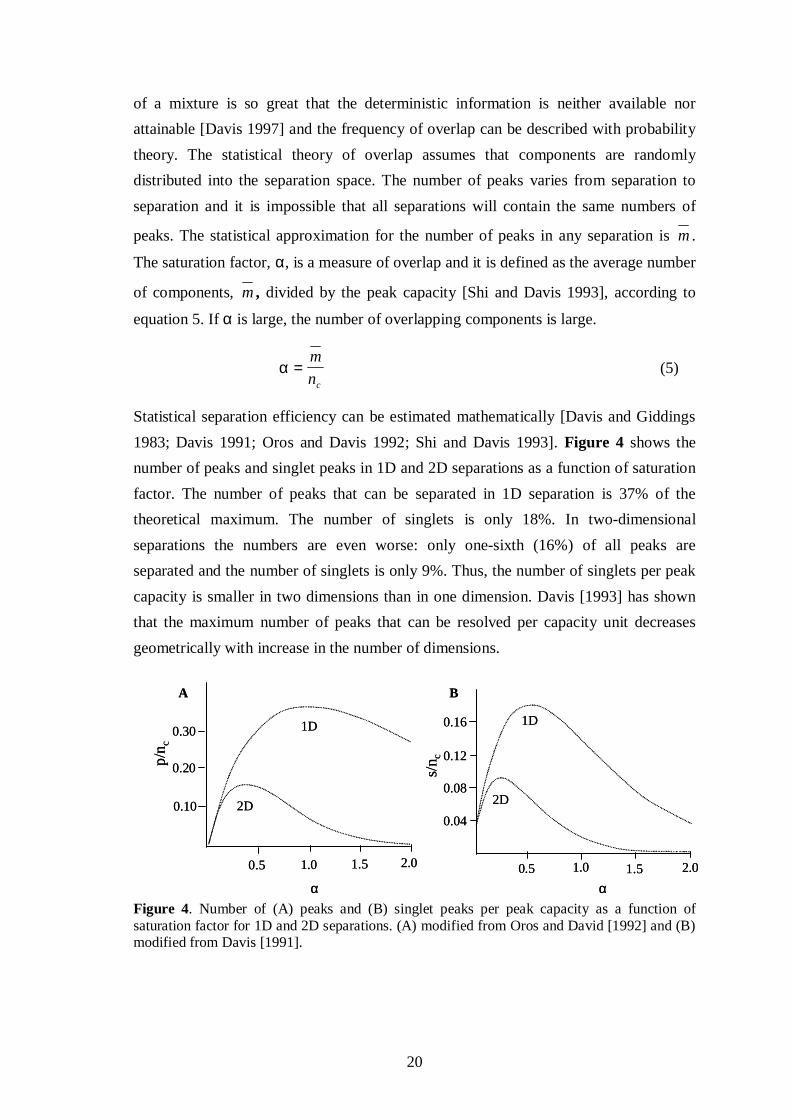
Statistical separation efficiency can be estimated mathematically [Davis and Giddings1983; Davis 1991; Oros and Davis 1992; Shi and Davis 1993]. Figure 4 shows thenumber of peaks and singlet peaks in 1D and 2D separations as a function of saturationfactor. The number of peaks that can be separated in 1D separation is 37% of thetheoretical maximum. The number of singlets is only 18%. In two-dimensionalseparations the numbers are even worse: only one-sixth (16%) of all peaks areseparated and the number of singlets is only 9%. Thus, the number of singlets per peakcapacity is smaller in two dimensions than in one dimension. Davis [1993] has shownthat the maximum number of peaks that can be resolved per capacity unit decreasesgeometrically with increase in the number of dimensions.

Figure 4. Number of (A) peaks and (B) singlet peaks per peak capacity as a function ofsaturation factor for 1D and 2D separations. (A) modified from Oros and David [1992] and (B)modified from Davis [1991].

0.5 1.0 1.5 2.0α

s/n c

0.04

0.08

0.12

0.16

B

2D

1D

0.5 1.0 1.5 2.0

α

p/n c

0.10

0.20

0.30

A

2D

1D

0.5 1.0 1.5 2.0α

s/n c

0.04

0.08

0.12

0.16

B

2D

1D

0.5 1.0 1.5 2.0

α

p/n c

0.10

0.20

0.30

A

2D

1D

21

The statistical evaluation shows that the available peak capacity is utilised lessefficiently in two dimensions than in one dimension [Oros&Davis 1992]. This can beexplained by the difference in component-free space around a singlet peak [Davis1991]: in 1D separation two component-free zones are required around the peak, whilein 2D, where a peak is considered as a circle, four zones are needed. The space demandfor singlet peak formatting simply is more stringent in two dimensions than in one, andthe separation space is not as efficiently used. This conclusion does not, however, meanthat 2D separations are inferior to 1D, since the peak capacity is much larger in 2Dseparations. This will now be explained.

When a 2D separation is orthogonal, i.e., the separation mechanisms in the twodimensions are independent of each other, the total peak capacity is calculated bymultiplying the peak capacities of the two dimensions (Equation 6a, Figure 5A). Inheart-cutting 2D systems, by comparison, the total peak capacity is the sum of the peakcapacities of the first and second dimensions (Equation 6b, Figure 5B).

n n nc c c≈ ×1 2 (6a)

21 ccc nnn +≈ (6b)

Figure 5. Visualisation of peak capacity in (A) comprehensive and orthogonal 2D techniquewhere the whole sample is subjected to the second column separation, and (B) heart-cutting 2Dtechnique, where only a few fractions are transferred to the second column separation.Modified from Bertch [1999].

For example, if nc1 = 200, which is typical for normal GC, and nc2 = 20, then the totalpeak capacity nc for the orthogonal separation is 4000. Lee et al. [2001] have calculatedthat a total peak capacity of 4000 would only be possible in one dimension with a platenumber of about 19 million in a column of inner diameter 0.25 mm and length about 4km (assuming 5000 plates per metre). Although long columns are possible in GC, this

B

1st-dimension retention

A

2nd-d

imen

sion

rete

ntio

n


B


A

2nd-d

imen

sion

rete

ntio

n


22

length is impossible in practice. The world´s longest GC column to date (presented atthe 29th International Symposium on Capillary Chromatography, Riva del Garda, Italy,May 29-June 2, 2006) is just 1321 m long.

In practice, the peak capacity of a GC×GC system can be approximated simply bycalculating how many peaks can fit into the total available separation space [Marriott2002]. Taking a peak as having a 15 s base width in the first dimension, 200 ms in thesecond dimension, and 60 min separation time with 4 s modulation period, we get apeak capacity nc1× nc2= 3600/15×4/0.2=240×20=4800. Although, as noted above, thiscapacity cannot be fully utilised, the potential peak capacity is dramatically increasedover that of a 1D separation. In a 1D system having peak capacity of 240 (as above), 43singlets (18% of 240) can be separated, while in the 2D system the number of singlet is10-fold, 432 (9% of 4800).

2.2.4 Structured chromatograms

A fourth feature of GC×GC is the structured nature of the 2D chromatograms, whichmeans that chemically related compounds are located close to each other and they formclearly visible groups. Often homologous series and their isomers, for example n-alkanes and their branched isomers, form so called roof-tile pattern (Figure 6)[Schoenmakers et al. 2000].

Figure 6. Drawing of a structured chromatogram and roof-tile pattern in a 2D GC×GC plot.Modified from Schoenmakers et al. [2000].

mono-aromatics

alkenes

linear&cyclicalkanes


2nd-d

imen

sion

rete

ntio

n mono-aromatics

alkenes

linear&cyclicalkanes


2nd-d

imen

sion

rete

ntio

n

23

The formation of structured chromatograms is explained by Giddings [1995] in termsof dimensionality. The dimensionality of a separation system, n, refers to the differentseparation stages. The dimensionality of a sample, s, in turn, is a measure of samplecomplexity and is the number of independent variables needed to separate samplecomponents. These variables, such as carbon number, molecular mass [Giddings 1995]and, especially in gas chromatography, boiling point and volatility [Phillips and Beens,1999a], vary in a systematic way.

Peak disorder in a chromatogram is dependent on the relationship between the systemsample dimensionalities [Giddings 1995]. (i) In the ideal case, n equals s (n = s) and allcompounds are separated. (ii) If the dimensionality of the sample is smaller than that ofthe system (n > s), additional separation space does not provide extra information andthe separation of the components may be correlated. (iii) If the dimensionality of thesample exceeds that of the system (n < s), components of the sample will not besystematically resolved in the system and the resulting separation will be disordered. Avolatility-based 1D gas chromatographic separation (n=1, s=3) of the compoundspresented in Figure 6 would result in the overlap of different chemical groups. AGC×GC separation with additional polarity-based separation in the second dimension(n=2, s=3) would resolve the different groups except for the linear and cyclic alkanes,for which polarity is not as strong a variable as for the other groups.

It needs to be noted that GC×GC analysis does not automatically provide structuredseparation. For example, chromatograms of atmospheric aerosol lack structure becauseof the wide variety of compounds and compound classes, which means that the sampledimensionality exceeds the system dimensionality [Hamilton et al. 2004].

2.2.5 Capability to detect low quantities

The capability to detect low quantities is a feature much in demand today. Use of athermal modulator, which concentrates fractions (see section 2.3.1.1) makes signalheight higher in GC×GC than in normal GC. Although noise is increased, too, owing tothe higher sampling rate, GC×GC can detect lower quantities than GC. Amplitudeenhancement has been modelled by Lee et al. [2001], who concluded that the increasewas from 15- to 25-fold with 4 and 5 s modulation periods. Enhancement is still greaterwith longer modulation period.

24

The lowest quantity that can be detected is reported as limit of detection (LOD). It isgood to note that intensity increase is not directly proportional to decrease in LOD.Moreover, use of the highest modulated fraction of the peak envelope slightlyunderestimates the LOD values for GC×GC. In the analysis of alkanes and aromaticsby GC and GC×GC Beens et al. [1998b] found that when the instrumentation wascapable of working at high data acquisition rate, the detection limit for GC×GC waslower than that for GC: 1D GC LOD 0.009% and GC×GC LOD 0.0005%. Truong et al.[2001] determined LODs for sterols and found that 1D GC LOD was 0.09 µg/ml whileGC×GC LOD was 0.02 µg/ml. Application of chemometrics to GC×GC data (obtainedwith a valve modulator) decreases LODs [Fraga et al. 2000b] owing to the efficientextraction of signal from noise.

2.3 Instrumentation and data analysis

An essential part of any GC×GC system is the modulator working between thecolumns. Analytical conditions must be carefully adjusted to achieve good separation,and programs dedicated to GC×GC are required for data analysis.

2.3.1 Modulators

The function of the modulator is to collect and transfer fractions from the first to thesecond column. It works throughout the analysis, transferring the whole sample fromthe first to the second column separation. The modulation period, i.e., the fractiontransfer interval is short, typically from 3 to 6 s. In view of íts essential role, themodulator is often called the heart of a GC×GC system. There are two types ofmodulators: thermal and valve modulators. Thermal modulators are further divided intoheated and cryogenic ones.

2.3.1.1 Thermal modulators

Compared with valve modulators, an important benefit of thermal modulators, bothheated and cryogenic, is that they concentrate fractions before their introduction to thesecond column separation. Injection band widths have been estimated to vary fromabout 10 to 60 ms [Adahchour et al. 2003a; Beens et al. 2001a], while the detectionband widths vary from tens to hundreds of milliseconds.

25

The first modulator in GC×GC was a two-stage thermal modulator (Figure 7A) [Liuand Phillips 1991], while the first commercial thermal modulator was a rotating slottedheater known as the Sweeper (Figure 7B) [Phillips et al. 1999b]. The application rangeof the Sweeper is from C9 to C30 [III], but it can be extended to n-alkane C40 if thethin-film modulator tube is heated in an independent temperature zone [Frysinger andGaines 2001]. There are also other designs based on thermal effects, such as the singlestage thermal modulator [de Geus et al. 1997], the thermal array modulator [Burger etal. 2003] and the electrically heated, air-cooled modulator [Libardoni et al. 2005].

Figure 7. GC×GC instrument with thermal modulators: (A) two-stage thermal modulator and(B) Sweeper.

The widest variety of modulators is found among the cryogenic thermal modulators,which rely on liquid nitrogen or carbon dioxide as trapping coolant. When nitrogen isused, additional heating is required to desorb the analytes from the trap; for carbondioxide, heated oven air is adequate. An important drawback of cryogenic modulatorsis the relatively large consumption of coolant.


Injector Detector

_+ +

A


Injector Detector

_+ +

A


Injector DetectorB


Injector DetectorB

26

The first cryogenic modulator was introduced in the 1990s. The effectiveness of thedevice was initially demonstrated as a solute trapping device [Marriott and Kinghorn1996; Marriott and Kinghorn 1997] and then it was adopted in GC×GC [Kinghorn andMarriott 1998]. This first device is known as a longitudinally modulated cryogenicsystem (LMCS) and, as the name indicates, it moves longitudinally along the column,up and down, to perform the modulation (Figure 8A). Application range is from C8 to40 [III].

A variety of other in-house built and modified cryogenic modulators have beenpresented including the semi-rotating cryogenic modulators developed in this study [I,II, VIII]. Beens and co-workers [Beens et al. 2001b; Dallüge et al. 2002b] modified theLMCS so that the coolant is sprayed directly on the column instead of into a separatedcylinder as in the original version. The application range was up to C40 [Beens et al.2001b]. They also introduced two non-moving designs: dual- [Beens et al. 2001a] andsingle-jet [Adahchour 2003a] modulators. In the dual-jet modulator (Figure 8B), twofixed jets alternately spray carbon dioxide onto the column. The application range ofthe modulator is from C8 to C30 [III]. In the single-jet modulator, one fixed jet sprayscarbon dioxide onto the column. Pursch et al. [2003] constructed a quad-jet systemcapable of modulating volatiles such as propane and butane with liquid nitrogen.Harynuk and Górecki [2003], in turn, designed a system based on liquid nitrogencooling, which is capable of trapping volatiles such as propane.

Commercial modulators include the quad-jet (KT2001) and the loop (KT2003,KT2004) modulators by Zoex (Houston, TX, USA) and the quad-jet modulator (LN2)by Leco (St. Joseph, MI, USA). All these modulators can use liquid nitrogen fortrapping analytes. The application range of the KT2001 is from C5 to C 30 [III], whilethat of the loop modulator is from C4 to C47 [Gaines&Frysinger 2004].

27

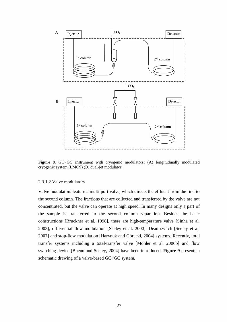
Figure 8. GC×GC instrument with cryogenic modulators: (A) longitudinally modulatedcryogenic system (LMCS) (B) dual-jet modulator.

2.3.1.2 Valve modulators

Valve modulators feature a multi-port valve, which directs the effluent from the first tothe second column. The fractions that are collected and transferred by the valve are notconcentrated, but the valve can operate at high speed. In many designs only a part ofthe sample is transferred to the second column separation. Besides the basicconstructions [Bruckner et al. 1998], there are high-temperature valve [Sinha et al.2003], differential flow modulation [Seeley et al. 2000], Dean switch [Seeley et al,2007] and stop-flow modulation [Harynuk and Górecki, 2004] systems. Recently, totaltransfer systems including a total-transfer valve [Mohler et al. 2006b] and flowswitching device [Bueno and Seeley, 2004] have been introduced. Figure 9 presents aschematic drawing of a valve-based GC×GC system.


Injector Detector

CO2

B


Injector Detector

CO2

B


Injector DetectorCO2A


Injector DetectorCO2A

28

Figure 9. GC×GC instrument with a valve-type modulator.

2.3.2 Analytical conditions

Successful performance of GC×GC analysis requires attention to column set, oventemperature and carrier gas flow rates and the detection system.

2.3.2.1 Columns

Columns used in GC×GC analyses can be divided into several categories according totheir polarity. The non-polar group includes 100% dimethyl polysiloxane and lowphenyl (mainly 5% phenyl) columns. Mid-polar columns include high phenyl (35-50%phenyl) and low cyano (6-14% cyano) columns. Polar columns include high cyano (>50% cyano) and trifluoropropyl and polyethylene glycol columns. Special columns arerepresented by chiral and liquid crystal phase columns and by sets where two differentcolumns are coupled together.

GC×GC studies since 1991 can be summarised by saying that the most commoncolumn in the first-dimension is a non-polar column containing either 100% dimethylpolysiloxane or 5% (di)phenyl–95% (di)methylpolysiloxane. The most commoncolumns in the second dimension are a semi-polar column containing 50% phenyl–50%methylpolysiloxane or a polar column containing 100% polyethylene glycol. Cyanocolumns are the third most common choice for the second dimension. Lately, (semi-)polar–non-polar column combinations have become popular, although the idea ofusing columns in this order is not new. In the first GC×GC paper, Liu and Phillips[1991] reported their use of a polyethylene column connected to a 100%


Injector Detector


Injector Detector

29

dimethylpolysiloxane column in the analysis of coal liquids. In this type of “reverse”set, a polyethylene glycol column is typically first and a non- or mid-polar columnsecond. Special column sets are used in the analysis of structurally related compoundssuch as polychlorinated biphenyls (PCBs).

Length of the first column is usually 20-30 m, the inner diameter 0.25 mm and the film

thickness 0.25 µm. The second column is typically shorter (1 m), the inner diameter is

narrower (0.1 mm) and the stationary phase is thinner (0.1 µm).

Although GC×GC set-ups typically consists of one first- and one second-dimensioncolumn, sometimes two second dimension columns have been utilised [Seeley et al.2001; Seeley et al. 2002; I; Bieri and Marriott 2006]. These require division of theeffluent after the first-dimension separation. Also a “twin” system with two first andtwo second columns has been demonstrated [Adahchour et al. 2005a].

2.3.2.2 Oven temperature ramp and carrier gas flow

Usually the two columns are placed into the same GC oven. Placing the second columninto a separate oven allows independent temperature programming. Linear temperatureprograms with isothermal steps at the beginning and end of the program are generally

applied. The ramp is typically 2–5 °C/ min, whereas in normal GC analysis it may be as

fast as 10–25 °C/min. Isothermal steps and varying ramps are needed in the GC×GCanalysis of structurally related compounds such as PCBs.

Since GC×GC columns with different inner diameters are connected in series,volumetric flow through the columns is the same but average linear velocities differs.In the basic column set-up (with no split vent placed at the column junction), the twocolumns cannot be operated at the optimum flow but compromises have to be made.Beens et al. [2005] showed that one column should be operated close to its optimumflow conditions, while a sub-optimum separation is accepted on the other column.Using a column set of 15 m×0.25 mm I.D. + 1.5 m×0.1 mm I.D and helium as carriergas, they demonstrated that separation quality along the second column was best underconditions where the second column was operated close to optimum. This requiredhead pressure of 200 kPa and resulted in flows of 9 cm/s in the first and 95 cm/s in the

30

second column. They also showed that use of a narrow bore second column (0.05 mmor even 0.10 mm) could result in very high velocities and therefore loss of plates.

By way of comparison, Kinghorn and Marriott [1998] reported flows of 20 and 200cm/s for a column set of 30 m × 0.25 mm I.D + 0.6 m × 0.1 mm I.D with helium ascarrier gas at head pressure of 152 kPa. Dallüge et al. [2002c] reported flows of 30 and230 cm/s with a column set of 15 m × 0.25 mm I.D. + 0.8 m I.D. × 0.1 mm with heliumas carrier gas. In this case volumetric flow was 1.3 ml/min.

2.3.2.3 Detection

Peaks eluting from the second column are narrow – from a couple of tens to hundredsof milliseconds – and acquiring enough data points per peak requires a fast detector.Typically, data acquisition rates are from 50 to 200 Hz. Flame ionisation detection(FID) is the most widely used technique owing to its good response to almost allorganic compounds and its suitability for quantitative analysis. Electron capture

detection (ECD) in µ-ECD mode is preferred in the analysis of halogenated

compounds. The inner volume of the detector in the µ-ECD mode is smaller than that in

normal configuration and the peak broadening is diminished. Increasingly popular ismass spectrometric detection. Use of time-of-flight mass spectrometry (TOFMS) is anattractive option since data can be acquired with high sampling rate range (50-500 Hz).Quadrupole mass spectrometry (qMS) is also possible, but then the speed aspectbecomes relevant. Compared with a TOF-mass spectrometer, a quadrupole instrumenthas a limited data acquisition rate. In combination with GC×GC, the best approach is tonarrow the mass range in order to obtain approximately 20 scans/s, which is consideredfast enough for qualitative analysis [Shellie and Marriott 2003a; Shellie et al. 2003b;III; Adahchour et al. 2005b; Korytar et al. 2005; Mondello et al. 2005; Cordero et al.2007]. Another option is to slow down the analysis, which, however, results inextremely long analysis time (e.g. 440 min [Frysinger and Gaines 1999]).

A few applications rely on element selective detection: nitrogen phosphorus detection(NPD) [Khummueng et al. 2006; Ryan et al. 2006; Ryan et al. 2005b; Mateus et al.2008] sulfur chemiluminescence detection (SCD) [Wang and Walters 2007; Ruiz-Guerrero et al. 2006; Blomberg et al. 2004; Wang et al. 2003] nitrogenchemiluminescence detection (NCD) [Adam et al. 2007; Wang et al. 2004] and atomic

31

emission detection (AED) [van Stee et al. 2003]. Another interesting application hasrecently been presented by d´Acampora Zellner et al. [2007], who coupled GC×GC toolfactometry (GC×GC-O) for odour fingerprinting. A recent review of detectors can befound in von Mühlen et al. [2006].

2.3.3 Data analysis

Any processing after the chromatographic analysis, needed to obtain the desiredinformation, is considered here as data analysis. Data analysis includes visualisation,comparative visualisation and qualitative and quantitative analyses of the data.

2.3.3.1 Visualisation

Visualisation begins with the slicing the raw chromatogram according to themodulation period and aligning of the slices parallel to each other (Figure 3). Parallellyaligned slices are transformed to a retention plane image in which the x-axis representsthe first-dimension separation and the y-axis the second-dimension separation. Thedetector response, i.e., intensity of the peak, is indicated with contours or colour scale.In a three-dimensional representation the z-axis indicates the detector response.Currently, GC×GC analysts use in-house written programs [e.g. Adam et al. 2007] forvisualisation as well as commercial software such as GC Image (Zoex, Houston, TX,USA), Transform (Fortner Software, Sterling, VA, USA), HyperCrom (ThermoScientific Waltham, MA, USA) or Pegasus (Leco, St. Joseph, MI, USA). In addition tothe mentioned visualisation, apex or bubble plots (also known as 3D surface plot) maybe used. In apex plots the peak maxima are indicated with dots and peak positions areclearly visualised. Apex plots fail to represent the resolution between individualcompounds, however. Bubble plots, in contrast, present the individual peaks, andbubble sizes correspond to total peak areas.

2.3.3.2 Comparative analysis

Since comprehensive two-dimensional separations provide information on the wholesample and its components, they are often used to characterise the differences betweensamples. A direct, qualitative approach is to compare 2D chromatograms by eye. Moresophisticated approaches are needed to express the differences quantitatively. Shellie etal. [2005] reported the use of difference chromatograms obtained by subtraction of two

32

2D plots in the metabolomic analysis of mouse tissue. Peak surfaces were normalised toexhibit minor differences in peak size. Hollingsworthy et al. [2006] introduced the termcomparative visualisation and presented the use of registration, i.e., retention timealignment, before subtraction of GC×GC plots. Also Tran and Marriott [2007]presented a subtracted 2D plot in a comparison of incense smoke and powder samples,but it is not clear whether the plot was created from a subtracted raw chromatogram orwhether the plots were subtracted after creation of the 2D plots. In addition tocomparative visualisation techniques, chemometrics has been used to locate differencesbetween samples [Mohler et al. 2006a; Pierce et al. 2006a-b]

2.3.3.3 Qualitative analysis

The primary interest in analytical chemistry is to identify compounds. Quantifyingthem is of secondary interest, and no reliable quantitative results can be obtainedwithout reliable identification, The procedures for identifying target analytes orunkowns in GC×GC are not much different from those in chromatography generally:

(i) Retention time comparison with standards when such are available

(ii) Standard addition, i.e., spiking the samples with standards

(iii) Comparison of the profiles of GC×GC(-FID) and GC-MS analyses

(iv) Coupling of GC×GC to mass spectrometry (quadrupole or more often time-of-flight instrument)

(v) Along with mass spectromentric detection linear retention indices aretypically used to confirm the identification, especially when the analytes areunknowns.

In addition, tentative identification can be made on the basis of a structuredchromatogram, as in the analysis of petrochemical samples.

When a GC×GC system is coupled to a mass spectrometer and especially a time-offlight instrument, the data sets that are generated are usually extremely large. Althoughmanual interpretation can be time-consuming, good results have been obtained in non-target analysis, i.e., identification of unknowns. Examples of the application ofGC×GC-TOFMS in qualitative analysis are given in Table 1. Typically, quality

33

parameters and retention indices were used to extract the relevant compounds from apeak table generated by the data processing. Extraction procedures were more or lessmanual, and no automated programs were needed except for the generation of the peaktables.

Several software routines have been proposed to handle and organise GC×GC massspectrometric data more efficiently. Location of the target analyte from amidst a vastamount of data has been rationalised with the DotMap algorithm [Sinha et al 2004a;Hope et al. 2005]. Welthagen et al. [2003] presented an alternative, group-typeprocedure based on GC×GC retention times and fragmentation patterns to classify(non-target) peaks into chemically related groups. Vogt et al. [2007] presented a similarprocedure, but they managed to dispense with the manual removal of sampling artifactsby increasing the peak finding criterion from S/N 40:1 to 100: 1. Availability ofautomated procedures would make GC×GC-TOFMS a more attractive tool.

Table 1. Identification criteria in GC×GC-TOFMS studies. S=similarity, R=reverse,P=probability.Number of identifiedcompounds / Matrix

Procedure Reference

152 / Tobacco smoke Quality parameters (S>800, R>900,S/N>30), retention indices (±15)

Dallüge et al.2002a

235 / Air Quality parameters (S>800, S/N>100),retention indices (±20)

Xu et al.2003

164 Volatiles / Honey Quality parameters (S>800, S/N>300),retention indices (±30)

Cajka et al.2007

56 monoterpenoids / Grape Quality parameters (S>850, S/N>500),EICs, retention indices

Rocha et al.2007

64 / Roasted barley Quality parameters (S>800,R>900,P>6000) manual inspection,retention indices

Bianchi et al.2007

50 Sulfur compounds / Rostedbeef aroma

Quality parameter (S>653?), simulatedretention indices

Rochat et al.2007

2.3.3.4 Quantitative analysis

Before quantitative analysis in chromatography, the relationship must be establishedbetween the amount of analyte and the chromatographic response. In traditional one-dimensional chromatography, quantitative analysis is usually straightforward since onecompound produces one peak, and either peak area or peak height can be used in thequantification. The situation is different in comprehensive two-dimensional techniqueswhere the relationship can be established using peak area, peak height or peak volume.

34

The total peak area of the modulated compound is a sum of the individual peaksgenerated by the modulation process. Peak height, either summed from individualpeaks or determined from a 3D plot, is rarely used since the peak envelope is affectedby the phase of the modulation [Ong and Marriott 2002]. Peak volume is commonlyused, especially in chemometric applications. In addition to single compounds,compound groups can be quantified. Group quantification is well known inpetrochemical analysis where chromatograms tend to be wellstructured.

Commercial software for quantitative GC×GC analysis is readily available: for exampleHyperChrom from Thermo Scientific, GC Image from Zoex and 4DGC×GC-TOFMSfrom Leco. Also in-house programs [Adam et al. 2007; Wang and Walters 2007;Shellie and Marriott 2003a; Ong et al. 2003] are used. The trilinear nature of GC×GCdata enables the use in quantification not only of traditional integration methods butalso chemometrics [Fraga et al. 2000a; van Mispelaar et al. 2003; Jonsson et al. 2004;Sinha et al. 2004b]. The number of quantitative analyses has increased, mainly due tothe introduction of commercial software packages.

Another important issue in quantitative GC×GC analysis is how matrix compounds andpossible overloading of the second column affect the quantification. The second

column in a GC×GC system typically has a very thin stationary phase (0.1 µm), and

because analyte fractions from the first column are focused into narrow concentratedbands, especially with cryogenic modulation, the second column may be overloaded ifexcessive amounts of solute(s) are injected. Overloading in a GC×GC analysis has beenshown to produce peaks that exhibit asymmetry in two dimensions (Figure 10),depending on the degree of overloading that arises from the solute in each dimension[Ong et al. 2001]. Peak contours for the overloaded compound express a shape that isnon-symmetric, and the peak maximum shifts to longer retention time in the dimensionthat is overloaded. Peak broadening will reduce the resolution and result in reducedpeak capacity. Since the second-dimension separation space is limited, any losses here,including those due to overloading, could seriously impair the performance of thesystem. The shifts in retention times make the identification more difficult. Moreover,overloading can cause problems in quantification, particularly when a non-specificdetector is used.

35

When a single compound or a mixture of compounds with equal concentration isresponsible for overloading in GC×GC, the sample can easily be diluted to anappropriate concentration. Often, however, the solutes responsible for overloading arenot the target analytes but matrix compounds. In environmental analysis, the sampleextracts will typically contain a large amount of unresolved matrix compounds, such asalkanes, while the target analytes are, perhaps, persistent organic pollutants. Dilutionwould not be an attractive option in this case, nor in general in trace level analysis. Analternative to sample dilution is to increase the sample capacity by using a second-dimension column with larger inner diameter. However, this would increase the deadtime in the second dimension and cause peak wrap-around [Harynuk et al. 2005]. Yet athird approach is selective clean-up, but as is often pointed out, the clean-up step couldbe omitted in GC×GC owing to the high separation efficiency. Although the effects ofoverloading are various, the issue has not been studied in detail.

Figure 10. Peak shapes of an overloaded and a normal GC×GC system. Modified from Ong etal. 2001.

A third issue closely related to quantitative analysis in GC×GC is mass transferbetween the two columns. When modulation is performed with a thermal modulatorthat concentrates the fractions, peak response measured as peak height is larger inGC×GC than in normal GC, but the peak areas are equal. Theoretically mass transferbetween the columns is 100%, and divergence from this value was studied in the earlyyears of modulator development and testing. Kinghorn et al. [2000], using alongitudinally modulated cryogenic system, reported a difference of 5% between theareas of GC (unmodulated) and GC×GC (modulated) peaks, while Phillips et al.[1999b], using a Sweeper modulator, found a difference of only 0.14%. Some valve-based modulation systems [Bruckner et al. 1998; Seeley et al. 2000; Seeley, et al.2007], it may be noted, do not produce quantitative mass transfer since only part of the

overloaded peak normal peak


2nd-d

imen

sion

rete

ntio

n

overloaded peak normal peak


2nd-d

imen

sion

rete

ntio

n

36

sample is introduced to the second column. However, if the peak areas of normal GCand GC×GC correspond to each other it should be possible to perform the calibrationfor GC×GC using normal GC runs. Substituting peak areas obtained by GC×GC intothe GC calibration would simplify the quantification procedure in terms of both labourand time.

2.4 Applications

According to van Mispelaar et al. [2005], chromatographic applications can beclassified into three groups: target-compound analysis, group-type separation, andfingerprinting. All three types can be qualitative or quantitative. Non-target analysis,i.e., identification of unknowns, can be added to the list as the fourth type ofapplication. GC×GC is currently used in the analysis of petrochemical, food,environmental, biological, essential oil and cosmetic samples. Selected applications arelisted in Table 2. Extensive reviews on GC×GC including applications have beenpublished by Dallüge et al. [2003] and Adahchour and co-workers [2006 a-d; 2008].

37

Table 2. Selected GC×GC applications: sample matrices, analytes, and system descriptions.Sample matrix / analytes 1st column 2nd column Modulator Detection Reference Environmental and relatedUrban aerosols 30 x 0.25 x 0.25 (BPX50) 1 x 0.1 x 0.1 (BPX1) Quad-jet (Leco) TOFMS Vogt et al. 2007Urban aerosols 30 x 0.25 x 0.25 (BPX5) 1.5 x 0.1 x 0.1 (BPX50) Quad -jet (Leco) TOFMS Welthagen et al. 2003Urban aerosol / Organics 10 x 0.18 x 0.18 (HP-5) 1.66 x 0.1 x 0.1 (DB1701) Quad -jet (Leco) TOFMS Hamilton et al. 2004Urban aerosols / Semi-VOCs 30 x 0.2 x 0.5 (RTX-1MS) 1 x 0.1 x 0.1(SolGelWax) Quad -jet (Leco) TOFMS Schnelle-Kreis et al. 2005Roadside nanoparticles 30 x 0.25 x 0.25 (BPX5) 1.0 x 0.10 x 0.10(BPX50) Loop (Zoex) TOF/qMS;NPD Ochiai et al. 2007Marine sediment / Pollutants 20 x 0.25 x 0.25 (DB-5) 1 x 0.1 x 0.1 (BGB-1701) Dual-jet (Beens) TOFMS Morales-Munoz et al. 2005Rural air / VOCs 30x 0.25 x 1 (DB-5) 1 x 0.1 x 0.1 (Carbowax) Quad-jet (Zoex) FID; TOFMS Xu et al. 2003Urban air / VOCs 50 x 0.53 x 5 (BP-1) 2.2 x 0.15 x 0.2 (BPX50) LMCS FID Lewis et al. 2000Cigarette smoke / VOCs 30 x 0.25 x 0.1 (DB-5) 1 x 0.1 x 0.1 (Carbowax) Quad -jet (Leco) TOFMS Dallüge et al. 2002aPCBs 10 x 0.15 x 0.1 (LC-50) 0.4 x 0.1 x 0.1 (BPX-5) LMCS FID Harju et al. 2001PCBs 10 x 0.1 x 0.1 (ChirasilDex) 1 x 0.1 x 0.1 (LC-50) LMCS µ-ECD Hagalund et al. 2001Toxaphenes 30 x 0.25 x 0.25 (HP-1) 1 x 0.1 x 0.1 (HT8) Sweeper µ-ECD Korytar et al. 2003 Fragrances, plants and essential oilsPerfume 30 x 0.25 x 0.25 (SLB-5) 0.75 x 0.1 x 0.1 (Swax10) LMCS FID&Olf.;qMS d´Ácampora Zellner et al. 2007Chrysanthemum / Pyrethrins 5 x 0.25 x 0.25 (BPX5) 0.3 x 0.15 x 0.15 (BPX50) LMCS FID Harynuk et al. 2006Essential oil of rose geranium 30 x 0.25 x 0.25 (HP-5) 0.5 x 0.32 x 0.25 (BP-20) LMCS qMS Shellie&Marriott 2003a FoodGrapes 60 x 0.25 x 1 (Equity-5) 2.5 x 0.1 x 0.1 (Swax10) Quad-jet (Zoex) TOFMS Rocha et al. 2007Honey / Volatiles 30 x 0.25 x 0.25 (DB-5MS) 1.25 x 0.1 x 0.1 (Swax10) Quad -jet (Leco) TOFMS Cajka et al. 2007Roasted beef / Sulfur volatiles 20 x 0.18 x 0.18 (DB-1) 1 x 0.1 x 0.1 (DB-225) Quad -jet TOFMS Rochat et al. 2007Roasted barley / Volatiles 30 x 0.32 x 0.5 (DB-WAX) 0.75 x 0.1 x 0.1 (BPX50) Dual-jet (Beens) TOFMS Bianchi et al. 2007Roasted coffee bean 30 x 0.25 x 0.25 (BPX5) 0.8 x 0.1 x 0.1 (BP20) LMCS NPD Ryan et al. 2006Can coating / Phenolic resins 30 x 0.25 x 0.15 (PS-255) 1.5 x 0.1 x 0.1 (SOP-50) DualJet(Thermo FID Biederman et al. 2006Wine / Methoxypyrazines 30 x 0.25 x 0.25 (BPX5) 1 x 0.1 x 0.1 (BP-20) LMCS NPD; TOFMS Ryan et al. 2005bOlive oil / FAMEs TWIN: 10x0.25x0.25 (BPX5)

& 25 x 0.32 x 0.25 (BP20)TWIN: 1x0.1x0.1 (BP20)& 1 x 0.1 x 0.1 (BPX-35)

Quad-jet (Zoex) FID Adachour et al. 2005a

PetrochemicalsDiesel fuel / Nitrogen comp. 30 x 0.25 x 1 (SPB-5) 3 x 0.25 x 0.25 (BPX50) Quad-jet (Zoex) NCD Wang et al. 2004Diesel / Sulfur compounds 30 x 0.25 x 1.0 (SPB-5) 3 x 0.25 x 0.25 (BPX50) Quad-jet (Zoex) SCD Wang et al. 2003Oil spill 3.5 x 0.1 x 3 (007-2) 1 x 0.1 x 0.14 (007-CW) Sweeper FID Gaines et al. 1999

38

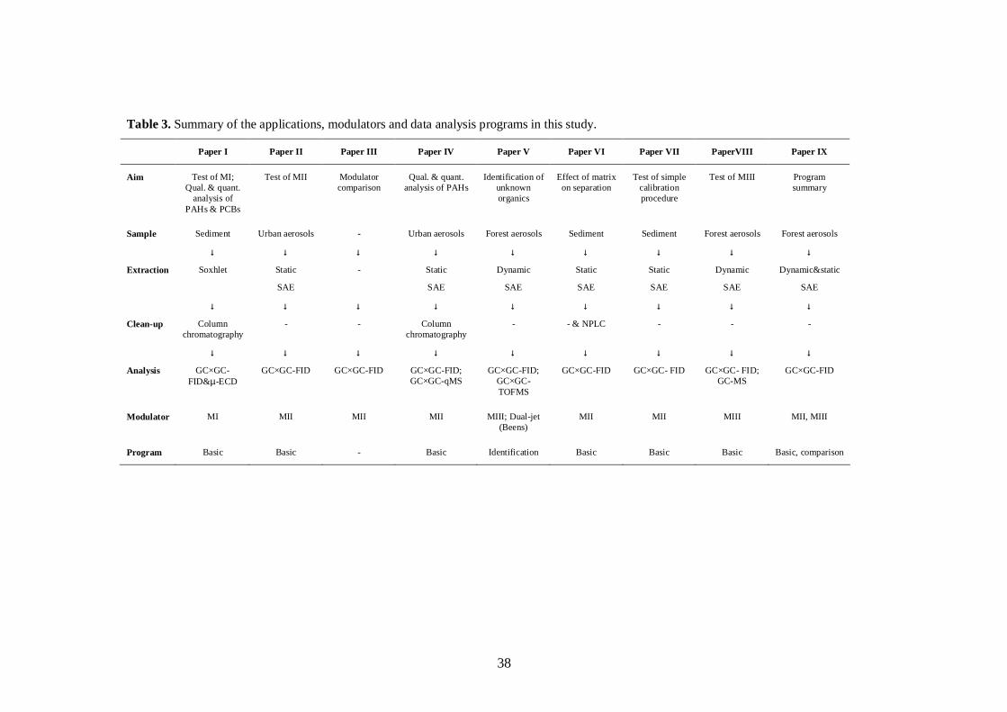
Table 3. Summary of the applications, modulators and data analysis programs in this study.

Paper I Paper II Paper III Paper IV Paper V Paper VI Paper VII PaperVIII Paper IX

Aim Test of MI;Qual. & quant.

analysis ofPAHs & PCBs

Test of MII Modulatorcomparison

Qual. & quant.analysis of PAHs

Identification ofunknownorganics

Effect of matrixon separation

Test of simplecalibrationprocedure

Test of MIII Programsummary

Sample Sediment Urban aerosols - Urban aerosols Forest aerosols Sediment Sediment Forest aerosols Forest aerosols

↓ ↓ ↓ ↓ ↓ ↓ ↓ ↓ ↓

Extraction Soxhlet Static

SAE

- Static

SAE

Dynamic

SAE

Static

SAE

Static

SAE

Dynamic

SAE

Dynamic&static

SAE

↓ ↓ ↓ ↓ ↓ ↓ ↓ ↓ ↓

Clean-up Columnchromatography

- - Columnchromatography

- - & NPLC - - -

↓ ↓ ↓ ↓ ↓ ↓ ↓ ↓ ↓

Analysis GC×GC-FID&µ-ECD

GC×GC-FID GC×GC-FID GC×GC-FID;GC×GC-qMS

GC×GC-FID;GC×GC-TOFMS

GC×GC-FID GC×GC- FID GC×GC- FID;GC-MS

GC×GC-FID

Modulator MI MII MII MII MIII; Dual-jet(Beens)

MII MII MIII MII, MIII

Program Basic Basic - Basic Identification Basic Basic Basic Basic, comparison

39

3 EXPERIMENTAL

Table 3 summarises the different parts of the study, reporting the aim, type of sample andanalytical procedure.

3.1 Chemicals and samples

Chemicals and samples used in the research are listed in Table 4. Sediment EC-1 wasselected as a model sample because it contains a large amount of matrix compounds inaddition to polycyclic aromatic hydrocarbons (and polychlorinated biphenyls) at certifiedconcentrations. Atmospheric aerosol samples were selected in view of their complexpattern of organic compounds, most of them present at trace level. Detailed informationon aerosol sampling can be found in papers II, IV and V.

3.2 Devices and columns

Devices and columns used in the research are listed in Table 5. The three modulators thatwere constructed are presented as schematic drawings in Figure 11 and their structuresare briefly described in the following text.

40

Table 4. Chemicals and samples used in the research.Chemical / sample Manufacturer / supplier Comment Paper4,4´-Dibromooctafluorobiphenyl Aldrich (Gillingham, U.K.) Internal standard I, IV-VII, IX2,2´-Binaphthyl AccuStandard (New Haven, CT, USA) Internal standard I, IV, IXn-Decane Fluka, Buchs, Germany Standard compound IIn-Hexadecane Fluka, Buchs, Germany Standard compound IIn-Octadecane Fluka, Buchs, Germany Standard compound IIn-Eicosane Fluka, Buchs, Germany Standard compound IIn-Tetracosane Fluka, Buchs, Germany Standard compound IIn-Hexacosane Fluka, Buchs, Germany Standard compound IIn-Octacosane Fluka, Buchs, Germany Standard compound IINaphthalene Fluka, Buchs, Germany Standard compound II2-Methylnaphthalene Fluka, Buchs, Germany Standard compound IIFluoranthene Fluka, Buchs, Germany Standard compound IIPyrene Fluka, Buchs, Germany Standard compound IIChrysene Fluka, Buchs, Germany Standard compound II

)-Verbenone Fluka, Buchs, Germany Standard compound IV9H-Fluorenone Fluka, Buchs, Germany Standard compound IVXanthone Fluka, Buchs, Germany Standard compound IVAcenaphthenequinone Fluka, Buchs, Germany Standard compound IV9,10-Anthracenedione Fluka, Buchs, Germany Standard compound IV2-Methylanthraquinone Fluka, Buchs, Germany Standard compound IVPhenanthrene-9-carboxaldehyde Fluka, Buchs, Germany Standard compound IV7H-Benz[de]anthracen-7-one Fluka, Buchs, Germany Standard compound IV5,12-Naphthacenedione Fluka, Buchs, Germany Standard compound IVβ-Nocaryophyllene aldehyde Synthesised in our laboratory, Parshintsev et al. 2008 Standard compound IXPAH mixture Z-014G-R AccuStandard (New Haven, CT, USA) 17 standard compounds I, IV-VIIIPCB mixture PCB-W22 AccuStandard (New Haven, CT, USA) 15 standard compounds IAlkane mixture DRH-001S-10X AccuStandard (New Haven, CT, USA) n-Alkanes from C10-C28 IV-VI, VIIIModulator test mixtures A-C Provided by M. Kristenson, Vrije Universiteit, NL III

41

Table 4. continuedChemical / sample Manufacturer / supplier Comment PaperIsooctane Rathburn Chemicals (Walkerburn, Scotland) Solvent, HPLC grade I, IIToluene Lab Scan Analytical Sciences (Dublin, Ireland) Solvent, HPLC grade I, V, VIn-Hexane Lab Scan Analytical Sciences (Dublin, Ireland) Solvent, HPLC grade II, IV-IXAcetone Lab Scan Analytical Sciences (Dublin, Ireland) Solvent, HPLC grade II, IV-VI, IXn-Heptane Fisher Scientific (Loughborough, UK) Solvent, HPLC grade IVDichloromethane Lab Scan Analytical Sciences (Dublin, Ireland) Solvent, HPLC grade VI, IXEthylacetate Lab Scan Analytical Sciences (Dublin, Ireland) Solvent, HPLC grade VISediment EC-1 National Water Research Institute (Burlington, CA) Certified reference material I, VI, VIIUrban aerosol samples - Collected in Helsinki II, IVForest aerosol samples - Collected in Hyytiälä V, VIII, IXCopper Merck (Darmstadt, Germany) Powdered, sample prep. IFlorisil Fluka, (Buchs, Switzerland) Particle size 60-100 mesh ISilica particles Waters (Milford, MA, US). Symmetrical, ∅ 5µm IVSilver nitrate (s) VWG International (Espoo, Finland) - IVSodium sulfate Fluka, (Buchs, Switzerland) IHelium AGA (Espoo, Finland) Carrier gas, purity 99.996% I-IXHelium Hoekloos (Schiedam, The Netherlands) Carrier gas, purity 99.999% VHydrogen AGA (Espoo, Finland) Carrier gas, purity 99.996% VHydrogen AGA (Espoo, Finland) Gas for FID I-IXAir Department´s compressed air system Gas for FID I-IXNitrogen AGA (Espoo, Finland) Make-up gas for FID,µECD I,Nitrogen AGA (Espoo, Finland) Make-up gas for FID II-IXNitrogen AGA (Espoo, Finland) Evaporating gas I, II, IV, VCarbon dioxide (l) AGA (Espoo, Finland) Cooling gas for modulation I-IXCarbon dioxide (l) Hoekloos (Schiedam, The Netherlands) Cooling gas for modulation V

42

Table 5. Devices and columns used in the research. Column dimensions are reported as length [m] × I.D. [mm] × film thickness [µm]. Apre-column was always used in front of the column set, but for brevity it is listed separately.Devices / columns Model and manufacturer / supplier Comment Paper

GC×GC-FID&µ-ECD;GC×GC-FID

HP 6890 GC (Agilent) III-IX

GC-qMS;GC×GC-qMS

HP 6890N GC-HP 5973 MSD (Agilent) VI, IVVIII,

GC×GC-TOFMS HP 6890 GC-Pegasus II TOFMS (Leco) VColumn set forGC×GC-FID&µ-ECD

Agilent Technologies (Espoo, Finland) +BGB Analytik, (Zürich, Switzerland)

20 m × 0.25 mm × 0.25 µm (HP-5MS) + 2×[ 0.7 m × 0.1 mm × 0.1 µm (BGB-Silaren)]

I

Column set for GC×GC-FID Agilent Technologies (Espoo, Finland) +BGB Analytik, (Zürich, Switzerland)

20 m × 0.25 mm × 0.25 µm (HP-5MS) +0.7-1 m × 0.1 mm × 0.1 µm (BGB-1701)

II, VIII

Column set for GC×GC-FID Agilent Technologies (Espoo, Finland) +SGE Europe (Milton Keynes, UK)

26.7 m × 0.32 mm × 0.25 µm (HP-1) +0.46 m × 0.1 mm × 0.1 µm (BPX-50)

III

Column set for GC×GC-FID Phenomenex (Torrance, CA, USA) +BGB Analytik, (Zürich, Switzerland)

20 m × 0.25 mm × 0.25 µm (ZB-5) +1 m × 0.1 mm × 0.1 µm (BGB-1701)

IV

Column set for GC×GC-qMS Phenomenex (Torrance, CA, USA) +BGB Analytik, (Zürich, Switzerland)

20 m × 0.25 mm × 0.25 µm (ZB-5) +1.2 m × 0.1 mm × 0.1 µm (BGB-1701)

IV

Column set for GC×GC-FID Agilent Technologies (Espoo, Finland) 20 m × 0.25 mm × 0.25 µm (HP-5MS) +0.5 m × 0.05 mm × 0.1 µm (Carbowax)

V

Column set for GC×GC-FID Agilent Technologies (Espoo, Finland)) 20 m × 0.25 mm × 0.25 µm (HP-5MS) +0.5 m × 0.05 mm × 0.1 (DB-17)

V

Column set for GC×GC-FID andGC×GC-TOFMS

Agilent Technologies (Espoo, Finland) +BGB Analytik, (Zürich, Switzerland)

20 m × 0.25 mm × 0.25 µm (HP-5MS) +0.7 m × 0.1 mm × 0.1 µm (BGB-1701)

V, IX

Column set for GC×GC-FID Agilent Technologies (Espoo, Finland) + BGB Analytik, (Zürich, Switzerland)

20 m × 0.25 mm × 0.25 µm (HP-5MS) +0.5 m × 0.1 mm × 0.1 µm (BGB-1701)

VI

Column set for GC×GC-FID Phenomenex (Torrance, CA, USA) 20 m × 0.25 mm × 0.25 µm (ZB-5) +0.7 m × 0.1 mm × 0.1 µm (ZB-1701)

VII

Column set for GC×GC-FID BGB Analytik, (Zürich, Switzerland) +Agilent Technologies (Espoo, Finland)

10 m × 0.25 mm × 0.25 m (HP-1701) +0.7 m × 0.10 mm × 0.12 m (HP-1)

IX

43

Figure 11. Structures of the semi-rotating cryogenic modulators.

Modulator I. The first version of the modulator (Figure 11) consists of a stainless steelshaft (O.D. 6.4 mm, I.D. 4.6 mm, 22 cm length), to which liquid CO2 is delivered fromthe top through a flexible polyetheretherketone (PEEK) capillary (O.D. 1.6 mm, I.D. 0.5mm). There is no casing around the shaft. Two nozzles (I.D. 0.17 mm) made of stainlesssteel capillary are soldered along the shaft at a 45º angle to each other. Coiled wireresistors (Kanthal, Vantaa, Finland, I.D. 0.5 mm) heated by electric current are installedto enhance the desorption step. The GC capillary is secured to the aluminium/stainlesssteel frame with two nuts and two vespel ferrules to avoid any vibration of the columndue to the cooling gas flow. The frame is attached to the wall of the GC oven. Themovements of the modulator and the power of the heaters are computer controlled with alaboratory-written C++ program. The shaft is rotated with a magnetic actuator(Shindengen, Camarillo, CA, USA) and the rotation angle is 45º.

40 m

m

45º

GC

CO2

Modulator I

25 mm180º

CO2

GC

Modulator II

30 mm180º

CO2

GC

Modulator IIIMotor Motor Motor

40 m

m

45º

GC

CO2

Modulator I

25 mm180º

CO2

GC

Modulator II

30 mm180º

CO2

GC

Modulator IIIMotor Motor Motor

44

Modulator II. The second version of the semi-rotating cryogenic modulator contains onlyone nozzle (I.D. 0.17 mm) from which CO2 is sprayed onto the column. A shaft made ofmetal tubing (O.D. 15 mm, I.D. 11 mm, length 18.5 cm) is fitted inside a casing ofstainless steel (I.D. 34 mm, O.D. 38 mm). A stainless steel transfer line (O.D. 0.8 mm,I.D. 0.5 mm) for liquid CO2 is led through the shaft and coiled inside the upper part of thecasing. The column is secured by a column holder, which holds it tightly and prevents itfrom vibrating during modulation. Contact of the column with metal is avoided byplacing septa between the metal parts of the holder and the column. The shaft is rotatedwith a permanent magnetic motor, which is computer-controlled with a laboratory-writtenC++ program. The rotation angle of the nozzle is 180°.

Modulator III. The third modulator resembles the second. There is only one 180° backand forth rotating nozzle (I.D. 0.17 mm or 0.25 mm) from which CO2 is sprayed onto thecolumn. The shaft of the third modulator is made of stainless steel tube (I.D. 4.6 mm,O.D. 6.4, length 23 cm) and it is fitted inside a casing (I.D. 24.5 mm; O.D. 25.5 mm)which is narrower than that of the second version. A stainless steel transfer line (O.D. 0.8mm, I.D. 0.5 mm) for liquid CO2 is coiled outside the shaft and the casing. The column isplaced on a stainless steel column holder in the same way as in the second design. Themost important new feature is that the shaft is rotated with a permanent magnetic motorwith gearhead (Igarashi Motors, IG 33 Type 0196-0020), which is controlled with amicrocontroller containing a quartz crystal. The micro-control program is written with Cand the graphical user interface with C++.

3.3 Data analysis

Data analysis programs used in the research are listed in Table 6. Operations of the in-house written programs are described in section 4.1.2.

45

Table 6. Data analysis programs used in the research.

Program Manufacturer Comment PaperChemStation Agilent Technologies, USA Data acquisition I- IXPegasus II software Leco, USA Data acquisition VIn-house written program Marriott, RMIT, Australia Conversion into 2D array VTransform Noesys, Crowthorne, UK Visualisation VIn-house written program Univ. of Helsinki, Finland Modulator control I-IXIn-house written program Univ. of Helsinki, Finland Visualisation&basic

oper.I-IX

In-house written program Univ. of Helsinki, Finland Comparison of 2D plots IXModde 4.0 Umetrics, Sweden Optimisation of DSAE VNIST MS library IV,V,VIII

3.4 Sample preparation

3.4.1 Soxhlet extraction

Soxhlet extraction was applied for sediment samples [I]. For extraction, 1 g of sedimentand 2 g of copper and sodium sulfate were mixed and refluxed with 80 ml of toluene for20 h. After the extraction the samples were concentrated in a rotary evaporator to 1 ml.

3.4.2 Static and dynamic sonication assisted extraction

Static sonication assisted extraction was applied for urban [II, IV] and forest aerosols[IX] as well as for sediment samples [VI, VII]. Urban aerosols were extracted with 3×10ml of n-hexane–acetone (1:1 v/v) for 30 min, and forest aerosols with 100 ml ofdichloromethane for 30 min. Sediment was extracted with various solvents, from whichn-hexane (100 ml, 30 min) was selected for the applications [VI, VII]. The excess solventwas evaporated under a gentle flow of nitrogen.

Dynamic sonication assisted extraction (DSAE) was applied for forest aerosols [V, IX].The extraction vessel was an empty polyetheretherketone (PEEK) column (length 50, 7.5mm I.D., Krotek, Finland), which was filled with pieces of filter samples and placed in anultrasonic bath. The extraction solvent was n-hexane–acetone (1:1, v/v), which waspumped through the vessel at a flow rate of 0.5 ml/min for 40 min. The excess solventwas evaporated under a gentle flow of nitrogen.

46

3.4.3 Sample clean-up procedures

Sample clean-up procedures are illustrated in Figure 12 and short descriptions are givenbelow. More detailed information can be found in the original papers [I, IV, VI].

Procedure 1 was applied for sediment samples [I]. It utilises column chromatographywhere a glass column is packed with Florisil (Fluka, Buchs, Switzerland) sandwichedbetween two layers of NaSO4. Gravity driven elution is done with 10 ml of isooctane.Finally, samples are concentrated to 1 ml with a gentle flow of nitrogen.

Procedure 2 was applied for urban aerosol samples [IV]. It utilises column

chromatography where an empty LC column is packed with 5 µm silver impregnated

silica, and mobile phase is driven through manually with a syringe. The non-polar

fraction is eluted with 200 µl n-heptane and the more polar fraction with 500 µl

dichloromethane. No further concentration is needed.

Procedure 3 was applied for sediment samples [VI]. It relies on normal phase liquidchromatography with ultraviolet detection (NPLC-UV). The column is an Ultrasphere(Beckman Coulter, Fullerton, CA, USA) silica column (25 cm×4.6mm I.D.) packed with

5µm particles. The eluent is n-hexane–ethyl acetate (95:5%, v/v) and it is pumped at flow

rate of 1 ml/min. UV detection wavelength is 254 nm. The non-polar fraction is collectedfrom 0 to 4 min and the PAH containing fraction from 4 to 8 min. The samples areconcentrated under a gentle nitrogen stream to a final volume of 0.5 ml.

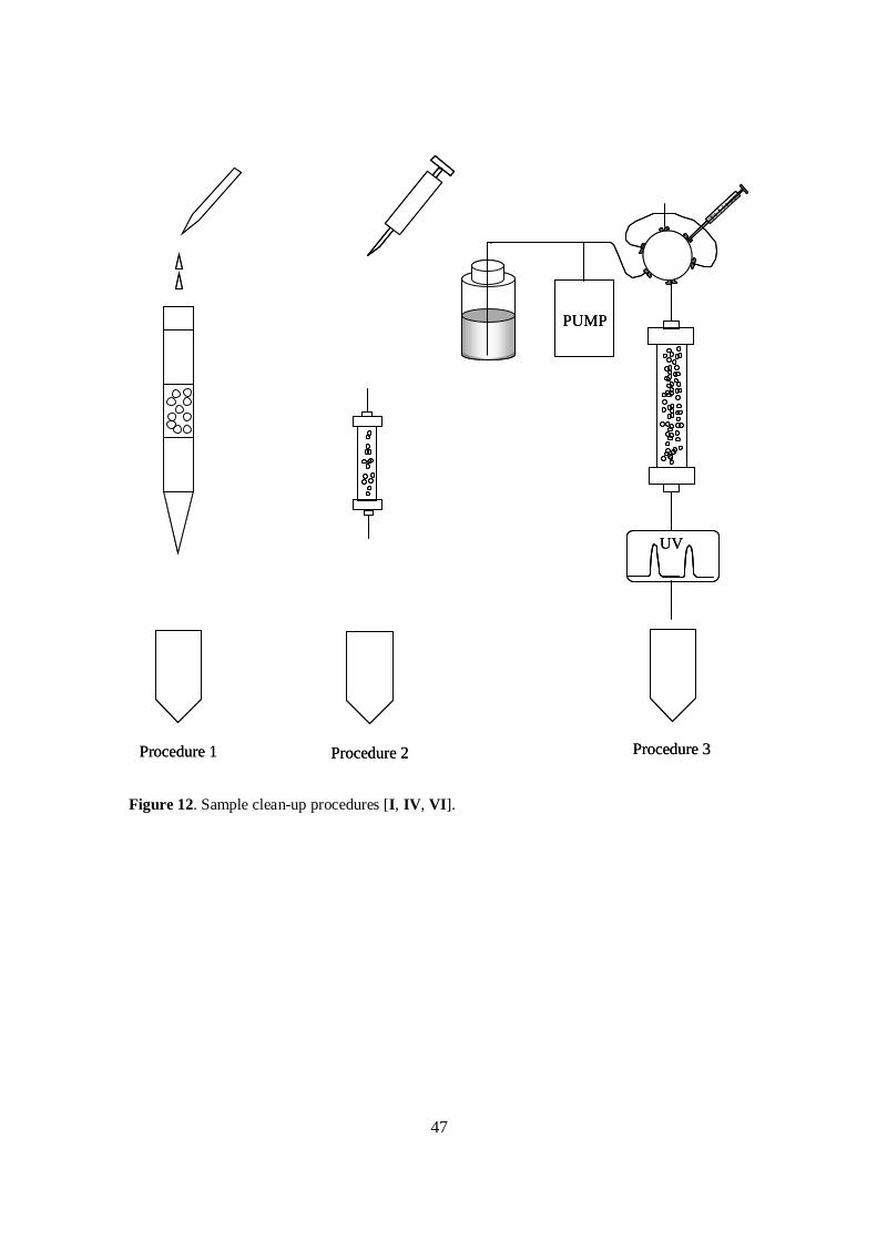
47

Figure 12. Sample clean-up procedures [I, IV, VI].

Procedure 1 Procedure 2

PUMP

UV

Procedure 3Procedure 1 Procedure 2

PUMP

UV

Procedure 3

48

4 RESULTS AND DISCUSSION

The results and discussion section is divided into two parts. The first part describes theinstrumental developments including the semi-rotating cryogenic modulators and in-house data analysis programs. The second part presents the methodological developmentcovering sample preparation, analytical conditions, and qualitative and quantitativeGC×GC analysis. Results of the analyses of sediment and aerosol samples reported in theoriginal papers are summarised and discussed.

4.1 Instrumental development

Three versions of a semi-rotating cryogenic modulator were constructed and tested interms of performance and modulation parameters (application range, retention timerepeatability and peak widths). Data analysis programs were created for the various tasksof the data analysis.

4.1.1 Development of the semi-rotating cryogenic modulator

There were several reasons for developing a new type of modulator. First, there were nocommercial cryogenic modulators available at the time the project commenced in theyear 2000. Secondly, moving parts (as in Sweeper and LMCS) were not desired aroundthe column because of the risk of breakage of the column if the modulator was notpositioned carefully. Thirdly, valves were not desired in the CO2 transfer line because ofpossible delays they might cause in the coolant spray.

Accordingly, all three versions of the semi-rotating cryogenic modulators rely on two-step cryogenic trapping with continuously flowing carbon dioxide (Figure 13). First, themodulator traps the fraction in position one. Then the nozzle is turned to position two,and the fraction is desorbed with heated wire resistors (modulator 1) or by oven air(modulators 2 and 3) and is re-trapped in the second position. Finally, when themodulator returns back to the first position, the fraction is released into the second-column separation. At the same time the trap in the first position prevents unmodulatedcompounds from entering the second column. All modulator designs allowed variation of

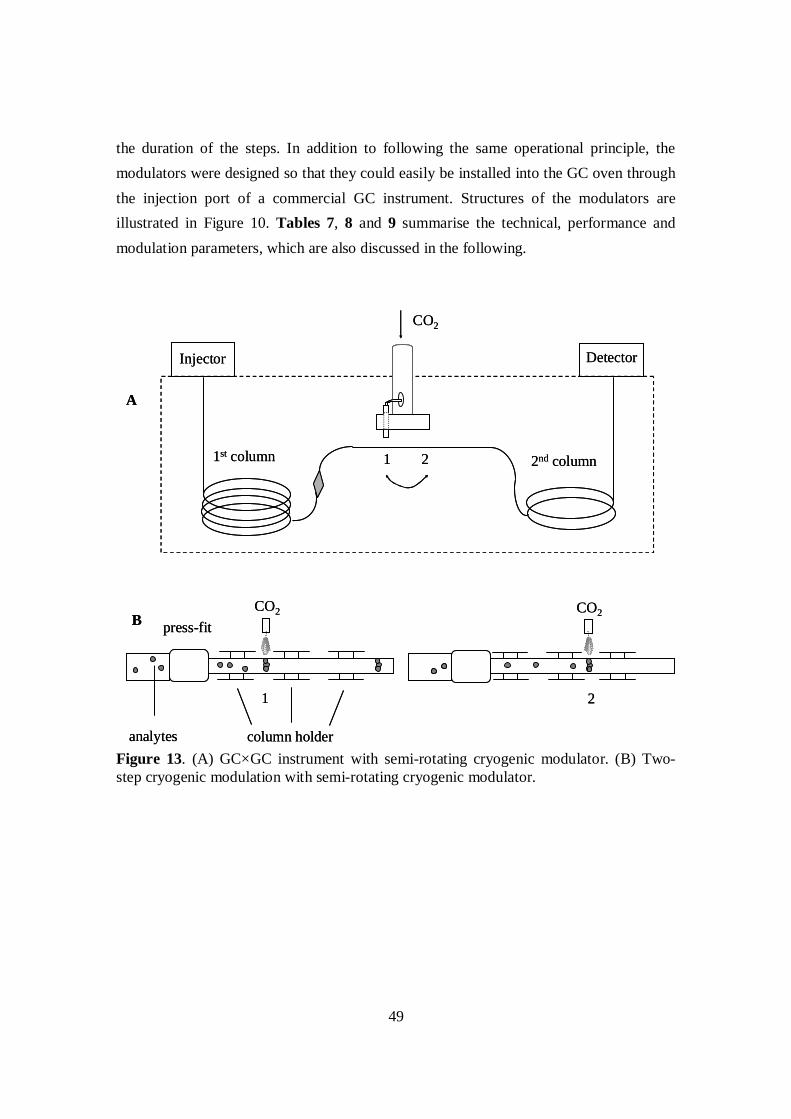
49

the duration of the steps. In addition to following the same operational principle, themodulators were designed so that they could easily be installed into the GC oven throughthe injection port of a commercial GC instrument. Structures of the modulators areillustrated in Figure 10. Tables 7, 8 and 9 summarise the technical, performance andmodulation parameters, which are also discussed in the following.

Figure 13. (A) GC×GC instrument with semi-rotating cryogenic modulator. (B) Two-step cryogenic modulation with semi-rotating cryogenic modulator.


Injector Detector

CO2

1 2

A

2

BCO2

press-fit

column holderanalytes

CO2

1


Injector Detector

CO2

1 2

A

2

BCO2

press-fit

column holderanalytes

CO2

1

50

Table 7. Technical parameters of the semi-rotating cryogenic modulators [I, II, VIII].Part Modulator I Modulator II Modulator IIIControl program C ++ C ++ Micro

controller,CTime file generated Yes Yes NoMotor Magnetic

actuatorPermanentmagnetic motor

Permanentmagnetic motorwith gearhead

Casing Material - Stainless steel Stainless steelI.D. - 34 mm 24.5 mmO.D. - 38 mm 25.5 mm

Column holder Material Stainless steel Aluminium Stainless steelColumn secured With nuts &

ferrules to frameBetween septa &plates

Between septa &plates

Shaft Material Stainless steel Stainless steel Stainless steelI.D. 3.9 mm 11 mm 4.6 mmO.D. 6.4 mm 15 mm 6.4 mmLength 22 cm 18.5 cm 23 cm

Shaft turn time Not measured ~ 40 ms ~200 msCO2 delivery tubing Material PEEK Stainless steel Stainless steel

I.D. 0.5 mm 0.5 mm 0.5 mmO.D. 1.6 mm 0.8 mm 0.8 mm

Nozzle I.D. 2 × 0.17 mm 0.17 mm 0.17; 0.25 mmTrap distance 40 mm 25 mm 30 mmAdditional heating Yes No No

Table 8. Performance parameters of semi-rotating cryogenic modulators [I, II, VIII]. * 2 smodulation period was the shortest tested.Parameter Modulator I Modulator II Modulator IIIApplication range C10-C28- C10-C34- C12-C34-1tRRSD [%]; 2s - 0.05 0.032tR RT RSD [%]; 2s - 10.3 1.51tR RT RSD [%]; 4s 0.14 0.03 0.012tR RT RSD [%]; 4s 3.1 3.7 1.6Selected step durations 70+30% 60+40% 60+40%Max. frequency at least 0.5 Hz * 1-3 Hz at least 0.5 Hz *CO2 consumption ~ 3 kg/h ~ 2 kg/h ~ 2-2.5 kg/h

51

Table 9. Modulation parameters [I, II, VIII]. Peak width at base (4σ), intensity increase relativeto GC and estimated LODs reported for selected n-alkanes and PAHs using the first (MI), second(MII) and the third (MIII) modulator with 4 s modulation period. *Universal press-fit after themodulator. **Y-shape press-fit after modulator, i.e., effluent divided between FID and µ-ECD.Compound Peak width at base [ms] Intensity increase LOD [pg/µl]

M I * M II M III M I ** M II M III M I ** M II M IIIC10 274 121 - 10 20 - 16 5 -C12 - - 75 - - 33 - - 6C16 258 123 87 9 19 40 16 4 5C18 289 135 103 - 20 22 15 6 10C26 408 148 125 7 21 33 20 5 7C28 - 166 131 - 14 33 - 8 7N 240 119 81 10 19 31 12 12 4Carb 292 - 111 10 - 25 19 - 5Flu 300 147 113 8 21 18 17 6 6Pyr 308 150 107 9 16 11 14 10 11Chry 345 160 125 9 17 19 16 23 6BghiPer 275 - 122 6 - 15 31 - 17Average 299 141 107 9 19 25 18 9 8

4.1.1.1 Structure and performance of the modulators

The first modulator (MI) contains two CO2 spraying nozzles at a distance of 40 mm andwire resistors to enhance desorption of the analytes (Table 7). The modulator controlprogram generates a time file, which contains exact times of modulation and which isused in the data analysis for slicing the raw chromatogram. Shaft turn time was notmeasured, but the maximum tested modulation frequency was 0.5 Hz (Table 8).Application range was tested only up to C28, but there is no reason why higher boilingpoint compounds would not elute from the column. Average repeatability of modulationtimes was good in the second dimension (3.1%). Modulation cycle step durations wereselected to be 70+30%, which means that in 4 s modulation period the first step lasts 2.8 sand the second 1.2 s. Consumption of carbon dioxide was 3 kg/h. Note that CO2 wasprayed from the two nozzles at the same time.

In comparing the modulation results (Table 9), note that the column set and columnconfiguration were different in the test of the first modulator and in the tests of the secondand third modulators (Table 5).

52

In the first modulator, additional heating with wire resistors was tested to enhance thedesorption of the analytes. The heating power of the wire resistors could be programmedfor heating time and heating power [I]. A study of the effect of heating on the peakshapes of PAHs and PCBs as model compounds showed that the peaks of PAHs were onaverage 25% higher and 20% narrower with heating. Though less dramatically, heatingalso improved the peak shapes of PCBs as was seen on in their improved symmetryfactors. Unfortunately, despite the positive effect of the wire resistors they also tended toburn the stationary phase of the column if overheated. In the early stages of the study aseparate modulation column (length 20 cm) was installed to the first part of the second-dimension column. Then, if the stationary phase was damaged due to overheating, onlythe modulation column needed to be changed. The columns in this construction wereconnected with universal class press-fit connectors, and the extra press-fit connector isthe reason why the peak widths for the analytes are much wider with the first modulator(240-345 ms) than the other two (Table 9). Later, the modulation column was fitted witha Y-type press-fit connector for joining to two second-dimension column: one leading to

an FID and the other to a µ-ECD. Since the effluent was divided after the modulator,

between FID and µ-ECD, the intensity increments (compared to unmodulated GC peaks)

were smaller and LODs higher than in the construction where the whole effluent wasdirected to one detector.

Although the first modulator version was rugged and worked well, two major problemswere encountered: relatively large consumption of carbon dioxide and the risk of the wireresistors overheating. The first version of the modulator was used in the analysis of PAHsand PCBs in sediment [I].

The second modulator (MII) was built with a view to diminishing the CO2 consumption.With the number of nozzles spraying CO2 reduced to one, the consumption of CO2 wasreduced from about 3 to 2 kg/h. The heated wire resistors were rejected as unnecessarysince the heated oven air was sufficient for desorption of the analytes. Other advantagesover the earlier modulator design were that the fine adjustment of the position of the CO2

spray was easier and more flexible. Also, the columns were easily installed and removed.

53

The distance between the trap positions was 25 mm. Shaft turn time was about 40 ms,and maximum modulation frequency was 2 Hz (Table 8). As for MI, the modulatorcontrol program for the second modulator generates a time file. Application range wastested only up to C34. Average repeatability of modulation times in the second dimension(3.7%) was good with a 4 s modulation period but poorer (10.3%) with a 2 s modulationperiod. Modulation cycle step durations were 60+40%, which means that in a 4 smodulation period, the first step lasts 2.4 s and the second 1.6 s.

Improvements in peak widths, peak intensities and LOD (Table 9) were largely due to thelack of press-fits and no division of effluent after the modulation. Peak widths at basevaried from 120 to 160 ms. LOD values were improved since the whole effluent wasdirected to the detector. Mass transfer studies (see paper II) showed the areas of theunmodulated (i.e. GC) peaks to correspond well to areas obtained by summing themodulated GC×GC peaks.

The only problem encountered with the second version is that the thin metal capillaryleading to the nozzle occasionally breaks and has to be changed. Otherwise, themodulator has been running reliably. The second modulator has been used in a widerange of applications [II, V-VII, IX, Hyötyläinen et al. 2002] and is still in use.

The third modulator (MIII) was built to improve the timing of the modulation. Themodulator control program of the third modulator was made independent of the computercontrolling the GC runs, and this improved the repeatability of the retention time in thesecond dimension. Further, it was constructed of commercially available materials andparts, and the structure was made simpler and lighter. Since the design was basically thesame as in the second modulator, consumption of CO2 and the modulation parameterswere at the same level as with the second modulator. The modulation cycle step durationswere again 60+40%.

The new control program for the modulator meant that time files were no longergenerated, and slicing of the raw chromatogram was performed with predetermined

54

modulation times. This improved the repeatability of the retention times markedly, andthe repeatability was no longer dependent on the length of the modulation period: RSDsfor the second-dimension retention times were 1.5% for 2 and 4 s modulation periods(Table 8). Replacing the permanent magnet motor with one with a gearhead slowed downthe rotation: turn time of the shaft was slightly below 200 ms, which is almost five timesslower than that of the second version. Slower rotation led to lower maximum modulationfrequency and narrower application range; thus, decane was no longer modulatedproperly. LOD values were on the same level as for the second modulator. Because thethird version was used in the analysis of semi-volatile organics in atmospheric aerosolparticles [V, IX], the narrower application range did not cause problems.

To conclude in regard to the technical findings in the modulator development, the fastestrotation and highest modulation frequency were achieved with the permanent magneticmotor used in the second version of the modulators. The most accurate modulation wasachieved when the motor was controlled with a microcontroller containing a quartzcrystal, as in the third version of the modulator. Additional heating in the desorption stepwas not necessary with CO2 as coolant.

An example of the performance of MIII is shown in Figure 14. The better sensitivity ofGC×GC is readily observed by comparing the chromatogram profiles obtained by GCand GC×GC. The intensity increase is notable and a particularly important feature whenthe compounds of interest are present at trace level.

55

Figure 14. Profiles of GC-FID and GC×GC-FID chromatograms of a forest aerosolsample [V]. Modulation was performed with MIII.

4.1.1.2 Comparison of modulators

As shown in Table 9, peak widths for n-alkanes and PAHs obtained with our second andthird modulators varied from 75 to 160 ms. Peak widths reported in the literature forsimilar compounds obtained by different modulators are reported in Table 10. Widths areon the same level as those of our systems.

100

200

300

100

200

300

GC-FID

GC×GC-FID100

200

300

100

200

300

GC-FID

GC×GC-FID

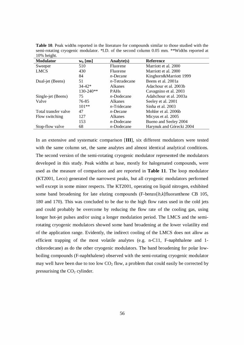
56

Table 10. Peak widths reported in the literature for compounds similar to those studied with thesemi-rotating cryogenic modulator. *I.D. of the second column 0.05 mm. **Widths reported at10% height.Modulator wb [ms] Analyte(s) ReferenceSweeper 510 Fluorene Marriott et al. 2000LMCS 430 Fluorene Marriott et al. 2000

84 n-Decane Kinghorn&Marriott 1999Dual-jet (Beens) 51 n-Tetradecane Beens et al. 2001a

34-42* Alkanes Adachour et al. 2003b130-240** PAHs Cavagnino et al. 2003

Single-jet (Beens) 75 n-Dodecane Adahchour et al. 2003aValve 76-85 Alkanes Seeley et al. 2001

101** n-Tridecane Sinha et al. 2003Total transfer valve 47 n-Decane Mohler et al. 2006bFlow switching 127 Alkanes Micyus et al. 2005

153 n-Dodecane Bueno and Seeley 2004Stop-flow valve 68 n-Dodecane Harynuk and Górecki 2004

In an extensive and systematic comparison [III], six different modulators were testedwith the same column set, the same analytes and almost identical analytical conditions.The second version of the semi-rotating cryogenic modulator represented the modulatorsdeveloped in this study. Peak widths at base, mostly for halogenated compounds, wereused as the measure of comparison and are reported in Table 11. The loop modulator(KT2001, Leco) generated the narrowest peaks, but all cryogenic modulators performedwell except in some minor respects. The KT2001, operating on liquid nitrogen, exhibitedsome band broadening for late eluting compounds (F-benzo[b,k]fluoranthene CB 105,180 and 170). This was concluded to be due to the high flow rates used in the cold jetsand could probably be overcome by reducing the flow rate of the cooling gas, usinglonger hot-jet pulses and/or using a longer modulation period. The LMCS and the semi-rotating cryogenic modulators showed some band broadening at the lower volatility endof the application range. Evidently, the indirect cooling of the LMCS does not allow asefficient trapping of the most volatile analytes (e.g. n-C11, F-naphthalene and 1-chlorodecane) as do the other cryogenic modulators. The band broadening for polar low-boiling compounds (F-naphthalene) observed with the semi-rotating cryogenic modulatormay well have been due to too low CO2 flow, a problem that could easily be corrected bypressurising the CO2 cylinder.

57

Table 11. Summary of peak widths obtained in a systematic comparison of modulators [III].Analyte M II Sweeper LMCS QuadJet

(KT2001)Dual-jet(Beens)

Loop(KT2003)

Undecanone (C11) 93 195 178 93 85 51Heptadecanone (C17) 110 170 76 68 68 51Triacontane (C30) 102 - 85 85 85 59

1-Chlorodecane 136 204 110 76 76 681-Chlorododecane 119 161 76 76 76 59F-Naphthalene 212 178 153 102 119 76F-Phenanthrene 136 153 119 119 136 85F-Benzo[b,k]fluoranthene 170 221 178 238 161 119

CB 28 & 31 119 144 110 119 102 68CB 77 127 153 127 136 119 76CB 153 127 170 110 127 110 68CB 105 119 170 136 153 127 76CB 180 127 204 119 204 110 68CB 170 136 - 144 212 119 76

4.1.2 Development of data analysis programs

Three types of programs were developed in this study [IX]. The first program allowsvisualization and basic operations such as determination of peak retention times and peakvolumes. The second program is designed for comparison of 2D plots by overlayingthem. These two programs are suitable for analysis of GC×GC data but also data obtainedby comprehensive two-dimensional liquid chromatography (LC×LC). Only the analysisof GC×GC data is discussed here. The third program is used for the identification ofunknowns and is meant for handling GC×GC data obtained from mass spectrometricdetection. Operations and relevant information on the programs are given in Table 12and presented below.

58

Table 12. Input files and operations of the developed data analysis programs. Operation CommentBasic

Input file A raw chromatogram as .csv fileBaseline fitting Manual break-line or automated polynomialSlicing According to a time file or predetermined MPVisualisation Original & baseline adopted raw

chromatograms, 2D contour & 3D colour plotsManual peak defining 1tR, 2tR, peak/peak group volumes and heightsAutomated peak defining 1tR, 2tR, peak volumes and heights

ComparisonInput files Two raw chromatograms as .csv fileBaseline fitting Manual break-line or automated polynomialSlicing According to a predetermined MPIntensity correction With area of selected compound, to raw signalOverlaying 2D plot Visualised as 2D contour plots in red&greenShifting of overlaid 2D plots Manually along 1st and 2nd dimension axesSubtraction of overlaid 2D plots Visualised as red/blue 2D contour plot

IdentificationInput files Original peak table, I libraries, I reference

retention times, quality parameters (minimumrequired similarity, S/N, maximum alloweddifference between Iexp and Ilit) and modulationparameters (PM and start time)

Data selection Based on quality parametersCalculation of I values Based on modulation parametersComparison of CAS numbersComparison of I values Based on predetermined allowed difference

4.1.2.1 Basic operations

The first program allows basic operations, which include baseline fitting, generation of2D and 3D plots and peak definding, i.e., determination of peak retention times, volumesand heights.

Baseline fitting to the raw chromatogram can be done automatically with a polynomialfunction or manually with a break-line. The latter is usually preferred because drifts in thebaseline level can then be followed accurately. After baseline fitting the rawchromatogram is sliced according to the actual or predetermined modulation period, andtwo- and three-dimensional plots are generated. Height is indicated in the 2D plot bycontours and in the 3D plot by colour scale. The visualisation procedure is shown inpaper IX (Figure 1).

59

Manual and automated peak defining are available. In manual peak defining, the userdefines a square around a peak, for which the program determines the retention times inthe first and second dimension and peak height and volume. Retention times and peakheight are related to peak apex, i.e., the highest fraction of the modulated peak envelope.Peak volume is calculated by multiplying the data point height by the underlying area andsumming these sub-columns of the peak together. Peak volume determination can also beused to find the peak volume for a compound group. Automated peak defining searchespeaks on the basis of a predetermined minimum peak height.

4.1.2.2 Comparison operations

The comparison program handles two files, of which one is the reference file and theother the data file. Functions of the program allow baseline fitting, intensity correction,adjustment of the position of the data files relative to the reference, and the subtraction ofpeak intensities.

Baseline fitting is done as in basic operations. If needed, intensity correction can beapplied to the raw signal using a correction factor obtained with use of a selectedcompound, usually an internal standard. Intensity correction with an internal standardhelps to overcome the problems of slight variation in sample volumes and possiblechanges in chromatographic conditions. Slicing of the raw chromatogram is carried outwith use of a predetermined modulation period. Overlaid chromatograms are shown as2D contour plots in different colours. Retention times can be scaled to match each otherby moving the data plots separately in the direction of the x- or y-axis. Best alignment isachieved when small regions are selected at a time, not the whole run. Finally, it ispossible to subtract overlaid runs from one another in order to compare concentrationdifferences.

An example of the operations is presented in paper IX, where two standard samples

containing β-nocaryophyllene aldehyde at different concentrations (0.5 and 1.5 µg/ml)

are compared. As the original data was not fully aligned, the data plot (red) was relocatedin the direction of the y-axis by shifting it upwards (Figure 3A) or downwards (Figure

60

3B) 0.15 s. After shifting, the reference plot (green) was subtracted from the data plot. InFigure 3A the colour of the contours is red because the subtraction is positive indicatingthat the concentration of analyte in the data is higher than that in the reference. In Figure3B the subtraction is negative indicating that concentration is higher in the reference.

Visual estimation of concentration differences was tested with samples collected inHyytiälä, Finland, during atmospheric new particle formation events (referred to as eventdays) and on days when formation did not occur (referred to as non-event days) [IX]. Theaim was to find out whether there were differences in chemical profiles of biogeniccompounds between the event and non-event days. Biogenic compounds, and especiallytheir oxidation products, were of special interest since they are believed to take part in thegrowth of newly formed aerosol particles. Special emphasis was put on pinonaldehyde,

which is an oxidation product of the α-pinene emitted by coniferous trees. Coniferous

trees make up the major part of the vegetation at the sampling site in Hyytiälä.

Six samples collected on event days and three on non-event days were analysed forpinonaldehyde. After intensity correction the data were compared by subtracting thevalues for non-event days from those for event days [IX] (Figure 5). Note that the peaksare not fully overlaid because of slight differences in peak shape. Blue peaks weredominant on most of the days, indicating the higher concentration of pinonaldehyde onnon-event days. Concentrations were more or less equal on March 17 and 22, but on noneof the days were red peaks dominant. Concentration of pinonaldehyde was concluded tobe higher on non-event than on event days during the period investigated. Concentrationdifferences determined with relative peak volumes fully supported the visual estimation.

4.1.2.3 Identification

An identification program was developed for GC×GC-TOFMS data obtained with Leco´sPegasus software, but it can be applied for other MS data of similar structure [V].

61

After data processing Pegasus produced a peak table containing maximum 9999candidates. Extracting the correct candidates involves removing compounds with lowsimilarity and signal-to-noise (S/N) values and further calculation and comparison ofretention indices with those in the library. Since the number of compounds after reductioncould still be several hundreds, manual calculations and comparisons were not considereda practical option, and a C++ program was written to ease data handling.

Input files are shown in Table 12. As output the program lists compounds that fulfil therequired criteria. From the original peak table the program accepts only those compoundsthat have similarity and S/N values above the predetermined values. The retention indicesare calculated on the basis of the first-dimension retention time. Finally, matches betweenChemical Abstract (CAS) numbers in the experimental and library data are searched andretention indices are compared.

4.2 Methodological development

Work comprised the development of sample preparation methods, selection of analyticalconditions and applications of those methods and conditions in qualitative andquantitative analysis of sediment and atmospheric aerosol samples.

4.2.1 Sample preparation

4.2.1.1 Dynamic sonication-assisted extraction

Dynamic sonication-assisted extraction was developed for the extraction of organiccompounds from filters on which aerosols samples were collected. The flow-rate andextraction time of the dynamic extraction were optimised using Modde 4.0 software(Umetrics, Umeå, Sweden) for factorial design. Five different combinations with bothextremes and one middle point were tested to achieve the best combination of flow-rateand extraction time. Best recoveries were obtained with low flow-rate (0.5 ml/min) andlong extraction time (40 min). DSAE was favoured for filter extraction because it issimple and fast and only small solvent volumes are needed. Because of the small solventvolume, it is easy to evaporate the solvent excess under a gentle stream of nitrogen, andsince a rotary evaporator is not required, less time is needed for the sample preparation.

62

DSAE was not applied for sediment samples. Filling the extraction vessel made of PEEKmaterial with the finely ground sediment mixed with sodium sulfate would easily haveresulted in particles left on the threads of the vessel and caused damage to the vessel orleakage. Sediment samples were more conveniently handled by Soxhlet [I] and staticsonication-assisted extractions [VI, VII].

4.2.1.2 Sample clean-up

Three different sample clean-up procedures were developed (Figure 12) and arecompared in the following.

Procedure 1. Procedure 1 was designed for sediment samples [I]. Sediment samplesrequired clean-up because (i) the Soxhlet extract contained high-boiling compounds thatwould not have eluted from the GC column, (ii) the amount of matrix compounds neededto be reduced to minimise peak overlap in the 1D GC analysis, which was beingcompared with the GC×GC analysis. For the clean-up procedure, Florisil was packed in aglass column sandwiched between layers of sodium sulfate, and the sample was elutedwith isooctane. Absolute recoveries were not determined but, as can be seen from Figure15, some non-polar compounds were present after clean-up.

Procedure 2. Procedure 2 was developed for the clean-up of urban aerosol samples [IV],

needed after preliminary studies indicated that quantification of PAHs and related

compounds might be affected by the presence of large amounts of (aliphatic) matrix

compounds. It was also assumed that the clean-up procedure would improve the

sensitivity of the method because a larger amount of sample could be injected to the GC

without the risk of overloading. A simple procedure relying on column chromatography

was developed. An empty LC column was packed in-house with 5 µm silver-impregnated

silica particles, and analytes were eluted with n-heptane and dichloromethane by forcing

the eluent through the column with a syringe. Although removal of the non-polar matrix

was good (97%), some matrix compounds remained in the sample, as can be seen from

Figure 16A. Recovery of the polar fraction (determined with standards) was 67%.

63

Figure 15. A sediment extract cleaned with procedure 1 [I]. Despite the cleaning non-polar bandcan be seen in the low part of the 2D plot. Influence of the non-linear temperature ramp appliedduring modulation appears as a wavy shape (see section 4.2.2.2).

Procedure 3. An NPLC system with ultraviolet detection was developed to further

improve the clean-up procedure for sediment samples [VI]. The NPLC system allows the

use of high efficiency columns, and the facility to monitor the separation with an HPLC

detector allows the conditions to be optimised quickly and precisely. Also, the fraction(s)

containing the analytes of interest can be accurately cut, unlike in column

chromatography (Figure 17). Procedure 3 proved to be superior to procedures 1 and 2.

The average removal percentage of n-alkanes was 97% for the standard solution and 70%

for the sample. Recovery of PAHs varied from 61 to 93% for standards and from 80 to

100% for samples. Typical contour plots from GC×GC analysis of cleaned and raw

sediment extract show the effectiveness of the HPLC fractionation (Figure 16B).

1st-dimension retention [min]

2nd-d

imen

sion

rete

ntio

n[s

]

15 25 35

1

2

3


2nd-d

imen

sion

rete

ntio

n[s

]

15 25 35

1

2

3

64

Figure 16. Effect of sample clean-up: (A) procedure 2 applied to urban aerosol [IV] and (B)procedure 3 applied to sediment [VI] extracts.

A BProcedure 2:cleaned aerosol extarct

Procedure 3:cleaned sediment extract

non-cleaned aerosol extract non-cleaned sediment extract


2nd-d

imen

sion

rete

ntio

n[s

]

35 45 55

1

2

35 45 55

1

2

35 45 55

1

2

3

35 45 55

1

2

3

A BProcedure 2:cleaned aerosol extarct

Procedure 3:cleaned sediment extract

non-cleaned aerosol extract non-cleaned sediment extract


2nd-d

imen

sion

rete

ntio

n[s

]

35 45 55

1

2

35 45 55

1

2

35 45 55

1

2

3

35 45 55

1

2

3

65

Figure 17. NPLC-UV chromatogram of a sediment extract [VI].

4.2.2 Analytical conditions

Successful GC×GC analysis requires the proper selection of columns, oven temperatureramp, carrier gas flow rate and detection.

4.2.2.1 Columns

Selection of the column set is critical in GC×GC. Most of the sets used in this work werenon-polar–semi-polar combinations (Table 5). The phase material of the non-polar first-dimension column was 5% (di)phenyl–95% (di)methylpolysiloxane. A columncontaining 14% cyanopropylphenyl–86% dimethylpolysoloxane (BGB or ZB-1701) wasa good choice for the second dimension since it separated PAHs well from matrixcompounds in the analysis of sediment and urban aerosol samples. Three differentsecond-dimension columns were tested in the analysis of forest aerosols. A column withthe phase most widely used in the second dimension, 50% phenyl–50%methylpolysiloxane, and an inner diameter of 0.05 mm, did not provide satisfactoryseparation efficiency because the flow rate of the carrier gas in the first column wasreduced due to the high back pressure caused by the second column. Apolyethyleneglycol (Carbowax) column was discarded mainly because of the limited

non-polar fraction0-4 min

polar fraction4-8 min

Time [min]840

UV

Res

pons

enon-polar fraction

0-4 minpolar fraction

4-8 min

Time [min]840

UV

Res

pons

e

66

temperature range. In the end, a 14% cyanopropylphenyl–86% dimethylpolysoloxanecolumn provided good separation. In the last study [IX], a reverse column set utilisingpolar–non-polar columns was used n the analysis of forest aerosols, since it provided abetter separation of biogenic compounds.

The use of non-polar–polar column sets is often defended on the grounds that it allows anorthogonal separation where volatility is the prevailing mechanism in the first dimensionand polarity in the second (see section 2.2.2). The mechanism in a polar–non-polarcolumn set is not much different, however, as shown in Figure 18 with n-alkanes andPAHs as model compounds. Only the retention order of compounds in the second columnis reversed. Although some mathematical approaches can be applied to achieveorthogonality (see section 2.2.2), a more practical approach to column selection is to tunethe separation so that a sufficient separation of target analytes or unknowns is obtainedand so that compounds are well scattered to the available separation space.

Figure 18. GC×GC-FID chromatogram of the separation of n-alkanes and PAHs on (A) non-polar–polar [V] and (B) polar–non-polar [IX] column sets. For PAHs abbreviations, see Table 17.Bb/kF = benzo[b/k]fluoranthene.

1st-dimension retention time [min]

A: HP-5MS + BGB-1701

C18 C20 C22 C24 C26 C28C16

Flu Pyr BaA/ChryPhe/Ant1.0

1.5

2.0

2.5

30 35 40 45

0.5

Bb/kF

2nd-d

imen

sion

rete

ntio

ntim

e[s

]

BaPyr

B: HP-1701 + HP-1

C16 C18 C20 C22 C24 C26 C28

Phe/Ant Flu Pyr BaA/Chry Bb/kF

30 35 40 45

BaPyr

1st-dimension retention time [min]


C18 C20 C22 C24 C26 C28C16


1.5

2.0

2.5

30 35 40 45

0.5

Bb/kF

2nd-d

imen

sion

rete

ntio

ntim

e[s

]

BaPyr

B: HP-1701 + HP-1

C16 C18 C20 C22 C24 C26 C28


30 35 40 45

BaPyr


C18 C20 C22 C24 C26 C28C16


1.5

2.0

2.5

30 35 40 45

0.5

Bb/kF

2nd-d

imen

sion

rete

ntio

ntim

e[s

]

BaPyr

B: HP-1701 + HP-1

C16 C18 C20 C22 C24 C26 C28


30 35 40 45

BaPyr

67

Table 13. Analytical parameters related to the column sets used in this study. Parameters used in calculations of the total peak capacities areaverage peak widths at base and the available separation space for the first and second dimensions. Temperature rates and head pressures arereported. Constant flow mode was applied except in study III (marked with asterisk *) where constant pressure was applied to generate aflow of 1.65 ml/min.

1D 2D TotalColumn set wb

[s]Time[min]

nc1 wb[ms]

PM[s]

nc2 nc Rate°C/min

Head pressure Paper

20 m × 0.25 mm × 0.25 µm (HP-5MS)+2×[0.7 m × 0.1 mm × 0.1 µm (BGB-Silaren)] 8 28 210 300 4 13 2800 5-10 200 kPa @ 40°C I

20 m × 0.25 mm × 0.25 µm (HP-5MS) +0.7-1 m × 0.1 mm × 0.1 µm (BGB-1701) 3 28 560 150 (2-) 4 27 14933 10 170 kPa @ 50°C II, VIII

26.7 m × 0.32 mm × 0.25 µm (HP-1) +0.46 m × 0.1 mm × 0.1 µm (BPX-50) 5 42 504 135 3 22 11200 5 100 kPa @ 50°C* III

20 m × 0.25 mm × 0.25 µm (ZB-5) +1 m × 0.1 mm × 0.1 µm (BGB-1701) 5 50 600 200 5 25 15000 5 170 kPa @ 60°C IV

20 m × 0.25 mm × 0.25 µm (HP-5MS) +0.7 m × 0.1 mm × 0.1 µm (BGB-1701) 3 45 900 200 3 15 13500 5 170 kPa @ 60°C V, IX

20 m × 0.25 mm × 0.25 µm (HP-5MS) +0.5 m × 0.1 mm × 0.1 µm (BGB-1701) 8 47 353 150 3 20 7050 5 100 kPa @ 60°C VI

20 m × 0.25 mm × 0.25 µm (ZB-5) +0.7 m × 0.1 mm × 0.1 µm (ZB-1701) 7 45 386 200 3 15 5786 3 125 kPa @ 60°C VII

10 m × 0.25 mm × 0.25 m (HP-1701) +0.7 m × 0.10 mm × 0.12 m (HP-1) 5 40 480 250 4 16 7680 5 150 kPa @ 60°C IX

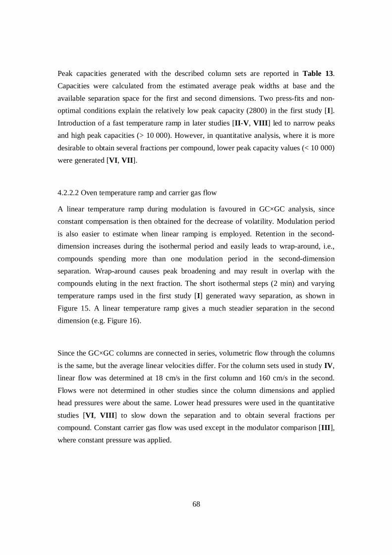
68

Peak capacities generated with the described column sets are reported in Table 13.Capacities were calculated from the estimated average peak widths at base and theavailable separation space for the first and second dimensions. Two press-fits and non-optimal conditions explain the relatively low peak capacity (2800) in the first study [I].Introduction of a fast temperature ramp in later studies [II-V, VIII] led to narrow peaksand high peak capacities (> 10 000). However, in quantitative analysis, where it is moredesirable to obtain several fractions per compound, lower peak capacity values (< 10 000)were generated [VI, VII].

4.2.2.2 Oven temperature ramp and carrier gas flow

A linear temperature ramp during modulation is favoured in GC×GC analysis, sinceconstant compensation is then obtained for the decrease of volatility. Modulation periodis also easier to estimate when linear ramping is employed. Retention in the second-dimension increases during the isothermal period and easily leads to wrap-around, i.e.,compounds spending more than one modulation period in the second-dimensionseparation. Wrap-around causes peak broadening and may result in overlap with thecompounds eluting in the next fraction. The short isothermal steps (2 min) and varyingtemperature ramps used in the first study [I] generated wavy separation, as shown inFigure 15. A linear temperature ramp gives a much steadier separation in the seconddimension (e.g. Figure 16).

Since the GC×GC columns are connected in series, volumetric flow through the columnsis the same, but the average linear velocities differ. For the column sets used in study IV,linear flow was determined at 18 cm/s in the first column and 160 cm/s in the second.Flows were not determined in other studies since the column dimensions and appliedhead pressures were about the same. Lower head pressures were used in the quantitativestudies [VI, VIII] to slow down the separation and to obtain several fractions percompound. Constant carrier gas flow was used except in the modulator comparison [III],where constant pressure was applied.

69

4.2.2.3 Detection

Four different detection techniques were tested: FID, ECD, qMS and TOFMS. They havedifferent features in term of speed. The flame ionization detector acquired data at a speedof 100 Hz, which means that 20 data points were obtained for a peak 200 ms at base.

Similarly, a 50 Hz sampling rate for the µ-ECD resulted in 20 data points over a 400 ms

PCB peak [I]. qMS operating at 18.94 scans/s gave 4-6 data points per 200 ms peak, andTOFMS operating at 50 Hz generated approximately 10 data points per 200 ms peak.

4.2.3 Qualitative analysis

Two approaches to identification were applied for compounds in aerosol samples:identification of target analytes [IV, VI, VII] and identification of unknowns [IV, V,VIII]. An overview of the procedures is presented in Table 14, with reference totechnique, analytes and applied procedure. Compounds identified in urban and forestaerosols are listed in Tables 15 and 16, respectively. Target-analyte procedures (retentiontime comparison and spiking) were applied for the sediment samples [I, VI, VII].

Table 14. Identification procedures for target and non-target (i.e. unknown) compounds inaerosol samples. β-NoCaA = β-nocaryophyllene aldehyde.Object Technique Analytes ProcedureTarget GC×GC-FID PAHs (IV)

β-NoCaA (IX)RT comparison, spikingSpiking, overlaying

GC×GC-qMS PAHs (IV) RT comparison,mass spectraNon-target GC×GC-FID&GC-MS Organics (VIII) Chromatographic profile, RI

GC×GC-qMS PAHs (IV) Library searchGC×GC-TOFMS Organics (V) Quality parameters, RI: Manual

and automated procedures

70

Table 15. Compounds identified and quantified in urban aerosols [IV].Targets [ng/m3] Non-targetsPhenanthrene/Anthracene 0.77 ± 0.06 TrimethylnaphthaleneFluoranthene 0.63 ± 0.07 MethylfluorenePyrene >5.48 ± 1.38 Methylanthracene/PhenanthreneBenzo[a]anthracene/Chrysene 1.28 ± 0.05 4H-cyclopenta[def]phenanthreneBenzo[k]fluoranthene 1.16 ± 0.11 MethylpyreneBenzo[a]pyrene 0.49 ± 0.12 11H-benzo[b]fluorineIndeno[1,2,3-cd]pyrene 0.67 ± 0.09 Cyclopenta[cd]pyreneBenzo[ghi]perylene 0.50 ± 0.07 Benzo[ghi]fluoranthene9,10-Anthracenedione 0.64 ± 0.16 C4-phenanthrene/Anthracene7H-Benz[de]anthracen-7-one 0.96 ± 0.33 Methylchrysene

9-PhenylanthracenePhenylmethylene-9H-fluoreneDimethylanthracenedione

Table 16. Compounds identified in forest aerosols [V]. M refers to manual identificationprocedure. Other compounds identified with automated search. * Tentative identified.Cyclic and oxygenated hydrocarbons (M) Acyclic alkanesα-Pinene 2,2,7,7-Tetramethyloctane3-Carene Undecane, 5-methyl-Eucalyptol Undecane, 2-methyl-Terpinolene * Dodecane, 3-methyl-Sabina ketone Tridecane, 4-methyl-Nopinone Tridecane, 3-methyl-Campholenic aldehyde *Camphor Acyclic alkenes4-Caranone 1-DodeceneIsomenthone * 1-TetradeceneVerbenoneBornyl acetate AldehydesPiperitenone * OctanalPinonaldehyde 2-Octenal2,5-Bornanedione * NonanalAlloaromadendrene Decanal

DodecanalAromatic hydrocarbonsBenzene, 1-methyl-4-(1-methylethyl)- KetonesBenzene, 1-methyl-3-(1-methylethyl)- 2-OctanoneBenzene, 1-methyl-2-(1-methylethyl)- 2-NonanoneBenzene, 1,3-diethyl- 2-DecanoneBenzene, 1-methyl-3-propyl- 2-UndecanoneBenzene, butyl- 2-TridecanoneBenzene, 1-ethyl-3,5-dimethyl-Benzene, 2-ethyl-1,3-dimethyl-Benzene, 4-ethyl-1,2-dimethyl-

71

Table 16. continued.Alcohols and acids1-Hexanol, 2-ethyl-Benzenemethanol, alpha,alpha-dimethyl-Benzenemethanol, alpha,alpha,4-trimethyl-Propanoic acid, 2-methyl-, 3-hydroxy-2,4,4-trimethylpentyl ester

OthersNaphthalene, decahydro-, trans-Naphthalene, decahydro-, cis-AcetophenoneBenzothiazoleHeptylcyclohexane2,5-Cyclohexadiene-1,4-dione, 2,6-bis(1,1-dimethylethyl)-

4.2.3.1 Identification of target analytes

GC×GC-FID. Target analysis by GC×GC-FID is most straightforward when standardsare available. Retention time comparison between standards and samples along withstandard addition (i.e. spiking) is a relatively good and reliable procedure since tworetention times are available and repeatability of retention times is generally good. Note,however, that the presence of matrix impacts negatively on the repeatability [VI] becausesmall changes in chromatographic behaviour affect the modulation phase and thus thesecond-dimension retention time. Standard addition is useful in such cases since thenchromatographic profiles can be compared in addition to retention times. Even though theseparation efficiency is high in GC×GC, co-elution may occur, and spiking can causeerroneous identification, as happened in the analysis of PAHs in urban aerosol [IV]. Twotarget compounds (dibenzo[ah]anthracene and 5,12-naphthacenedione) were tentativelyidentified by GC×GC-FID with retention time matching and spiking, but the presence ofthe compounds could not be confirmed with mass spectrometric detection (GC×GC-qMS). In most cases, however, the reliability of retention time comparison and spiking inthe identification can be considered good.

Standard addition became an even more attractive aid in identification after the programallowing overlay of two 2D plots was developed. As illustrated in paper IX (Figure 4),

trace amounts of β-nocaryophyllene aldehyde could then be identified in an forest aerosol

sample. Identification of trace level components with one-dimensional techniques wouldhave been challenging because, as can be seen from the 2D plot, severe overlap with the

72

non-polar compounds would have resulted. Combining spiking and overlaying improvesthe identification procedure.

Identification of unknowns is not possible with GC×GC-FID alone, though structuredchromatograms allow tentative identification of a compound or compound groups on thebasis of their location in the 2D plot. Tentative identifications were not attempted in thiswork since environmental samples, and especially aerosols, contain so many compoundgroups that sample dimensionality exceeded dimensionality of the method.

GC×GC-qMS. The scanning rate of the quadrupole mass spectrometer is slow, and whenit is coupled to GC×GC the only way to obtain enough data points per peak is to narrowthe scanned mass range or slow down the analysis. In this study [IV], the mass range wasnarrowed, since the aim was to compare GC×GC-FID with GC×GC-qMS analyses. Thenumber of scans per peak varied from 4 to 6 and the peak shape therefore become slightlyangular (Figure 19). GC×GC-qMS was used as a confirmatory technique in theidentification of PAHs in urban aerosols, and the tentative identification with GC×GC-FID was either confirmed or discarded. For most of the target analytes GC×GC-qMSconfirmed the identification, but three compounds (9H-fluorenone,dibenzo[ah]anthracene and 5,12-naphthacenedione) were discarded. Note, thatquantification is not possible with GC×GC-qMS owing to the low scanning rate.Identified target compounds are reported in Table 15, along with their atmosphericconcentrations determined by GC×GC-FID.

Figure 19. Extracted ion chromatogram of the main fraction of the fluoranthene standardobtained by GC×GC-qMS [IV].

100000

200000

300000

400000

500000

240 ms

Abu

ndan

ce

100000

200000

300000

400000

500000

240 ms

Abu

ndan

ce

73

4.2.3.2 Identification of unkowns

GC×GC-FID and GC-MS. Comparison of GC×GC-FID and GC-MS chromatograms (astotal ion chromatogram, TIC) was preliminarily studied as a method of identifyingunknown organic compounds in forest aerosol samples [VIII]. Since the chromatographicconditions were not identical in the two methods, an acceptable match of thechromatographic profiles was obtained in only a small region at the beginning of thechromatograms. The poor match elsewhere was due to co-elution and low sensitivity ofGC–MS in TIC mode. With I values used to confirm the identity, several compoundswere identified in the region between n-dodecane and n-tridecane. The reliability of theprocedure could be improved by applying identical analytical conditions for GC×GC-FIDand GC-MS.

GC×GC-qMS. The GC×GC-qMS technique was tested in the identification of otherpossible aromatic compounds than the target analytes in urban aerosols by subjecting thedata to library search [IV]. Although GC×GC-qMS worked well in the confirmation oftarget analytes, the limited number of data points and relatively low matches with libraryspectra reduced the reliability of the identification procedure for unknowns. As in thetarget analyses, quantification was not possible. The tentatively identified PAHs arereported in Table 16.

GC×GC-TOFMS. The GC×GC-TOFMS technique was used in the identification ofunknown organic compounds in atmospheric aerosol collected in Hyytiälä [V]. Thedeveloped automated identification procedure (section 4.1.2.3) was compared withmanual search.

Manual search is feasible when the compounds of interest are well defined. Althoughlaborious and time-consuming, manual search allows the researcher to use common sensein deciding whether a library hit is reasonable. It also allows an evaluation of theintensities of the fragments in spectra. Although intensities of the main fragments shouldremain constant with electron impact ionisation, there were minor discrepancies in theintensities between sample and library spectra. Manual search was carried out by

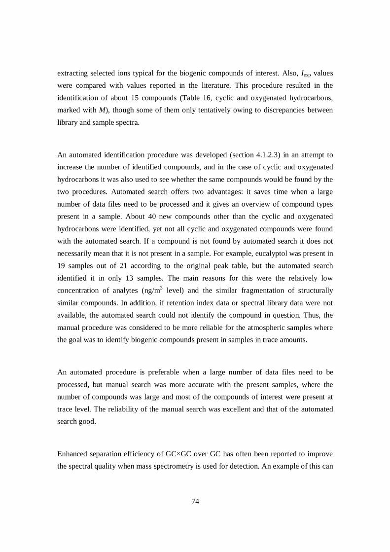
74

extracting selected ions typical for the biogenic compounds of interest. Also, Iexp valueswere compared with values reported in the literature. This procedure resulted in theidentification of about 15 compounds (Table 16, cyclic and oxygenated hydrocarbons,marked with M), though some of them only tentatively owing to discrepancies betweenlibrary and sample spectra.

An automated identification procedure was developed (section 4.1.2.3) in an attempt toincrease the number of identified compounds, and in the case of cyclic and oxygenatedhydrocarbons it was also used to see whether the same compounds would be found by thetwo procedures. Automated search offers two advantages: it saves time when a largenumber of data files need to be processed and it gives an overview of compound typespresent in a sample. About 40 new compounds other than the cyclic and oxygenatedhydrocarbons were identified, yet not all cyclic and oxygenated compounds were foundwith the automated search. If a compound is not found by automated search it does notnecessarily mean that it is not present in a sample. For example, eucalyptol was present in19 samples out of 21 according to the original peak table, but the automated searchidentified it in only 13 samples. The main reasons for this were the relatively lowconcentration of analytes (ng/m3 level) and the similar fragmentation of structurallysimilar compounds. In addition, if retention index data or spectral library data were notavailable, the automated search could not identify the compound in question. Thus, themanual procedure was considered to be more reliable for the atmospheric samples wherethe goal was to identify biogenic compounds present in samples in trace amounts.

An automated procedure is preferable when a large number of data files need to beprocessed, but manual search was more accurate with the present samples, where thenumber of compounds was large and most of the compounds of interest were present attrace level. The reliability of the manual search was excellent and that of the automatedsearch good.

Enhanced separation efficiency of GC×GC over GC has often been reported to improvethe spectral quality when mass spectrometry is used for detection. An example of this can

75

be seen in Figure 20. In GC–MS analysis, the small peak of alloaromadendrene isoverlapped by the peaks of alkanes or alkenes (not shown in Figure 20A) and dodecanal,and the GC–MS spectral match (649) is low because of the many interfering fragments.The additional separation column in the GC×GC-TOFMS analysis improves theseparation, and alloaromadendrene is clearly separated from less polar components, andmore importantly, from more polar dodecanal. The spectral match is improved to 801,and also the intensity pattern is closer to that of the library spectrum (see, e.g., fragments105 and 189).

Figure 20. Improvement of spectra of alloaromadendrene: extracted ion chromatogram and massspectrum obtained (A) by GC-MS and (B) by GC×GC-TOFMS. (C) is the NIST library spectrum[V].

50 70 90 110 130 150 170 190 210

50

61

65

74

79 94

105

119

135

148

161

177

189204

Dodecanal

DodecanalA

B

C

50 70 90 110 130 150 170 190 210

50

61

65

74

79 94

105

119

135

148

161

177

189204

50 70 90 110 130 150 170 190 210

50

61

65

74

79 94

105

119

135

148

161

177

189204

Dodecanal

DodecanalA

B

C

76

4.2.4 Quantitative analysis

Certified sediment (EC-1) [I, VI, VII] and urban aerosol [IV] samples were analysed

quantitatively by GC×GC-FID and GC×GC-µ-ECD.

The amounts of PAHs and PCBs in sediment EC-1 were determined to test thequantitativeness of the method [I] (see Corrections to the original papers). The amountsof PAHs differed somewhat from the certified values mainly due to the sample clean-upprocedure, which was originally developed for PCBs. The amounts of PCBs were inmuch better agreement with the reference values; only two measurements (PCB 52 andPCB 149/110) were out of range. Two further quantitative studies of the sedimentexamined the effect of matrix [VI] and a simple calibration procedure [VII] (see sections4.2.4.2 and 4.2.4.3).

The amounts of PAHs determined in urban aerosol extracts (Table 15) were inaccordance with the amounts given in the literature for other urban sites. Note thatamounts determined in aerosol extracts were lower than the amounts determined insediment extracts (see Table 17 for calibration range).

4.2.4.1 Calibration procedures

Correlation coefficients of the external calibration curves for PAHs (Table 17) werecalculated to identify the best way to perform quantitative GC×GC analyses. Curves forGC×GC analyses were constructed with peak volumes [I, IV, VI] and heights [I]determined with the new in-house program, and with summed peak areas [I, VI, VII] andheights [I], integrated with standard GC integration software and summed in spreadsheetprogram. In addition, normal 1D GC calibrations were performed with peak areas [I,VII]. In the first study [I], correlation coefficients for peak heights were found to belower than those for volumes and areas. This was as expected since the peak height ismore dependent on the modulation phase than are the other parameters. Even slightchanges in the chromatographic conditions will effect the shape of the peak envelope andthereby the peak height. Hence, only peak volumes and summed areas were utilised in thefurther studies [IV, VI, VII].

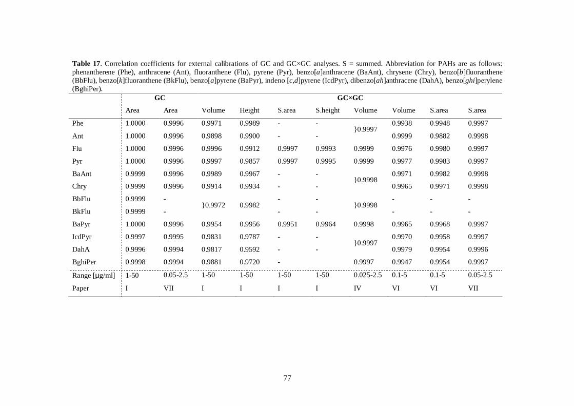
77

Table 17. Correlation coefficients for external calibrations of GC and GC×GC analyses. S = summed. Abbreviation for PAHs are as follows:phenantherene (Phe), anthracene (Ant), fluoranthene (Flu), pyrene (Pyr), benzo[a]anthracene (BaAnt), chrysene (Chry), benzo[b]fluoranthene(BbFlu), benzo[k]fluoranthene (BkFlu), benzo[a]pyrene (BaPyr), indeno [c,d]pyrene (IcdPyr), dibenzo[ah]anthracene (DahA), benzo[ghi]perylene(BghiPer).

GC GC×GC

Area Area Volume Height S.area S.height Volume Volume S.area S.area

Phe 1.0000 0.9996 0.9971 0.9989 - - 0.9938 0.9948 0.9997

Ant 1.0000 0.9996 0.9898 0.9900 - -}0.9997

0.9999 0.9882 0.9998

Flu 1.0000 0.9996 0.9996 0.9912 0.9997 0.9993 0.9999 0.9976 0.9980 0.9997

Pyr 1.0000 0.9996 0.9997 0.9857 0.9997 0.9995 0.9999 0.9977 0.9983 0.9997

BaAnt 0.9999 0.9996 0.9989 0.9967 - - 0.9971 0.9982 0.9998

Chry 0.9999 0.9996 0.9914 0.9934 - -}0.9998

0.9965 0.9971 0.9998

BbFlu 0.9999 - - - - - -

BkFlu 0.9999 -}0.9972 0.9982

- -}0.9998

- - -

BaPyr 1.0000 0.9996 0.9954 0.9956 0.9951 0.9964 0.9998 0.9965 0.9968 0.9997

IcdPyr 0.9997 0.9995 0.9831 0.9787 - - 0.9970 0.9958 0.9997

DahA 0.9996 0.9994 0.9817 0.9592 - -}0.9997

0.9979 0.9954 0.9996

BghiPer 0.9998 0.9994 0.9881 0.9720 - 0.9997 0.9947 0.9954 0.9997

Range [µg/ml] 1-50 0.05-2.5 1-50 1-50 1-50 1-50 0.025-2.5 0.1-5 0.1-5 0.05-2.5

Paper I VII I I I I IV VI VI VII

78

4.2.4.2 Effect of matrix on the separation

Separation of PAHs in sediment sample was studied [VI] to determine the effect ofmatrix components on quantitative trace GC×GC analysis. The second-dimension columnwas overloaded by progressively increasing the amount of matrix compounds and thechromatographic parameters were evaluated. The test samples were prepared byfractioning the sediment extracts by NPLC (clean-up procedure 3) and combining severalfractions of aliphatic matrix compounds with fixed amounts of PAHs. In the quantitativeanalysis, several calibration methods were tested for two types of samples: for rawextracts and extracts that had been cleaned by NPLC.

Increasing the amount of matrix 16-fold did not disturb the separation of PAHs in termsof peak width, asymmetry or resolution, but the depth of the valley between the PAH andthe preceding matrix peak increased and the repeatability of retention times slightlydecreased. Increase in peak-to-valley ratio was 38-fold at the maximum. The averagestandard deviation of total retention times of PAHs increased with matrix amount: in thepure solution it was 0.7 s (n = 5); in the moderate amount of matrix 1.1 s (n = 4) and inexcessive amount of matrix 2.5 s (n = 5). In general in GC×GC, small changes inchromatographic conditions affect the phase of the modulation and shift the position ofthe main peak, and this influences the total retention time. The GC×GC system seems tobe even more prone to the peak shifts in the presence of excessive amount of matrix

With fixed amount of PAHs (0.05 µg), the repeatabilities of peak areas and volumes

reasonable when the amount of matrix was moderate (area RSD 8%; volume RSD 11%),but the decline is marked when the amount of matrix was excessive (area RSD 16%;volume RSD 23%). For standards, areas and volumes were equally repeatable (area RSD7%; volume RSD 8%).

As reported in Figure 21 and paper VI (Table 3), the repeatability of the final resultsvaried between 10% and 31%. The best repeatability was obtained for external areacalibration (10%). RSD values were larger for volume calibration, especially for the non-cleaned sample (26–31%). It needs to be emphasised that the quantification was carried

79

out at trace level, which in many respects explains the large standard deviations. Largestandard deviations for trace level quantification have previously been reported byKorytar et al. [2005]. When the amount of (spiked) PAHs in the standard additioncalibration was increased, the repeatability of the peak volume determination improveddramatically (RSDs below 5%).

Figure 21. Effect of matrix on external (ex) and standard addition (add) calibrations for (A)cleaned and (B) non-cleaned sediment extracts determined by GC×GC-FID [VI]. PAH valuesreported as µg/g. Columns marked with asterisk lie outside of ± one standard deviation of thereference. For PAH abbreviations, see Table 17.

The number of out of range results (indicated with an asterisk in Figure 21) was greatestwhen area calibration was used. This is partly explained by the smaller standard

0

5

10

15

20

25

30

35

Phe Flu Pyr BaAnt Chr BaPyr IcdPyr BghiPer

[ug/

]

Certified

Area_ex

Area_add

Volume_ex

Volume_add

** ** **

A

0

5

10

15

20

25

30

35


[ug/

]

Certified

Area_ex

Area_add

Volume_ex

Volume_add

* * * * * * * ** * *

B

0

5

10

15

20

25

30

35


[ug/

]

Certified

Area_ex

Area_add

Volume_ex

Volume_add

** ** **

A

0

5

10

15

20

25

30

35


[ug/

]

Certified

Area_ex

Area_add

Volume_ex

Volume_add

* * * * * * * ** * *

B

80

deviations in the area calibration than in the volume calibration. The area calibrationseemed to underestimate the amounts of PAHs, and too low amounts were determinedespecially for compounds, that eluted in the end part of the chromatogram or thatappeared as isomers. In the end of the chromatogram column bleed and late elutingimpurities disturbed the separation (indeno[1,2,3-cd]pyrene–benzo[ghi]perylene).Isomers, in turn, were poorly resolved in the first column (phenanthrene–anthracene;benzo[a]anthracene–chrysene). The underestimation could also be explained bydifficulties in accurately defining the start and end of the peak, i.e., the exact location ofthe first and last fractions of the compound. Combining the correct fractions in a standardanalysis is relatively easy, but doing the same for a complex sample is much moredifficult, even when standard addition is used to ease the task. Neither calibration methodrelying on areas (neither external nor standard addition) worked satisfactorily at tracelevel. Problems were especially acute with non-cleaned samples (Figure 21B), whereonly the PAHs present in highest concentration (fluoranthene and pyrene) were within thegiven ranges for reference values.

Results obtained with volume calibration were well within the given ranges. Themagnitude of the results varied both below and above the reference values, but only threedeterminations lay outside the defined ranges. In general, sample clean-up was irrelevantto the results. In terms of the defined ranges, the external calibration provided resultscloser to the reference values than did the standard addition calibration. An advantage ofvolume quantification is that determining peak volumes from the two-dimensionalcontour plot with the software of this study is easier and more straightforward thansumming the areas from the raw chromatogram.

The quality of the separation was not significantly disturbed in terms of peak width,asymmetry or resolution when the amount of matrix was increased. However, the depthof the valley between the PAH and the preceding matrix peak increased with an increasein the amount of matrix, and the repeatabilities of retention times, peak areas andvolumes decreased. In quantitative analysis, calibration with areas showed a tendency tounderestimate the trace amounts of PAHs, especially for non-cleaned samples. In the case

81

of volume calibration, the most accurate results were obtained with external calibration,for both cleaned and non-cleaned samples.

4.2.4.3 Simplified calibration procedure

Total (100%) mass transfer between the two GC×GC columns was demonstrated in thetest of the second version of the semi-rotating cryogenic modulator [I]. This, and theresults reported above (section 4.2.4.2) showing that matrix does not disturbquantification when working above trace level, led us to test whether GC×GC areacalibration could be replaced by normal GC calibration [VII].

The calibrations were done in two ways using peak areas. The GC calibration was doneusing one-dimensional, normal GC analysis, where the peak area was readily obtained byintegrating of the signal with GC software. The GC×GC calibration involved a procedurewhere individual fractions were integrated with the same GG software and then summedup manually in a spreadsheet program to obtain the total area of the analyte peak.Samples were analysed only by GC×GC, and summed areas were substituted into the GCand GC×GC calibration equations.

Unmodulated and modulated areas corresponded well at various concentrations.Calibration curves were linear over the calibration range for both GC and GC×GC, withcorrelation coefficients above 0.998 in all cases. There were no statistical differences inthe slopes of the calibration curves (Student´s t-test, confidence level 1%). Since thecalibration curves were similar, also the final results were alike. As can be seen in Figure22 and in paper VII (Table 1), both the GC and the GC×GC calibrations gave resultsconsistent with the certified values when standard deviations in the measurements weretaken into account. Exceptionally, the amount of anthracene was overestimated in bothcalibrations. A similar result with a different analytical system was obtained previously[Lüthje et al. 2004]. Repeatabilities of the determinations were on the same level: relativestandard deviations were 11% for GC and 12% for GC×GC. The average LOD and LOQs

were 0.02 and 0.04 µg/ml for the GC method and 0.003 and 0.006 µg/ml for GC×GC.

The values for GC×GC are thus about one-tenth of those for GC. The difference can be

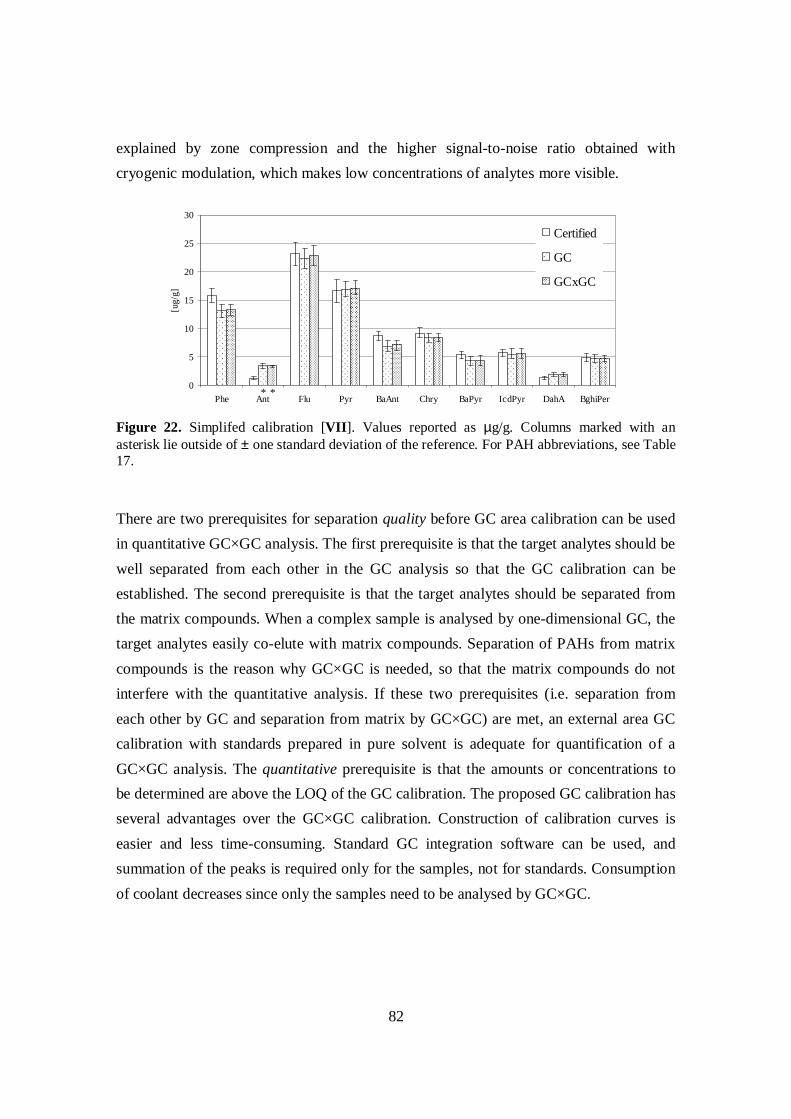
82

explained by zone compression and the higher signal-to-noise ratio obtained withcryogenic modulation, which makes low concentrations of analytes more visible.

Figure 22. Simplifed calibration [VII]. Values reported as µg/g. Columns marked with anasterisk lie outside of ± one standard deviation of the reference. For PAH abbreviations, see Table17.

There are two prerequisites for separation quality before GC area calibration can be usedin quantitative GC×GC analysis. The first prerequisite is that the target analytes should bewell separated from each other in the GC analysis so that the GC calibration can beestablished. The second prerequisite is that the target analytes should be separated fromthe matrix compounds. When a complex sample is analysed by one-dimensional GC, thetarget analytes easily co-elute with matrix compounds. Separation of PAHs from matrixcompounds is the reason why GC×GC is needed, so that the matrix compounds do notinterfere with the quantitative analysis. If these two prerequisites (i.e. separation fromeach other by GC and separation from matrix by GC×GC) are met, an external area GCcalibration with standards prepared in pure solvent is adequate for quantification of aGC×GC analysis. The quantitative prerequisite is that the amounts or concentrations tobe determined are above the LOQ of the GC calibration. The proposed GC calibration hasseveral advantages over the GC×GC calibration. Construction of calibration curves iseasier and less time-consuming. Standard GC integration software can be used, andsummation of the peaks is required only for the samples, not for standards. Consumptionof coolant decreases since only the samples need to be analysed by GC×GC.

0

5

10

15

20

25

30

Phe Ant Flu Pyr BaAnt Chry BaPyr IcdPyr DahA BghiPer

[ug/

g]

Certified

GC

GCxGC

* *0

5

10

15

20

25

30

Phe Ant Flu Pyr BaAnt Chry BaPyr IcdPyr DahA BghiPer

[ug/

g]

Certified

GC

GCxGC

* *

83

5 CONCLUSIONS

The GC×GC research summarised in this thesis comprised of the development ofmodulators and data analysis programs and the development and application of GC×GCmethods for the qualitative and quantitative analysis of environmental samples.

Three different versions of a semi-rotating cryogenic modulator were constructed andtested for their performance, application range and ruggedness. All the modulatorsworked well, and their performance was comparable to that of other in-house andcommercial modulators.

Three programs were developed for data analysis. The first program, covering basicoperations, allowed visualisation and reliable determination of the parameters needed inqualitative and quantitative analysis. The overlaying feature of the comparison programproved to be useful in the comparison of 2D plots. The identification proceduredeveloped for GC×GC-TOFMS data allowed the handling of large data sets in much lesstime than is required for manual processing, and it was shown to perform well in theanalysis of highly complex forest aerosol samples.

Sample preparation with dynamic sonication assisted extraction was successfully testedin the extraction of atmospheric aerosol collected onto filters. Benefits of the techniqueare fast and simple operation, low consumption of solvent and no need to evaporate theexcess of solvent after extraction. For sample clean-up, NPLC with UV detection provedsuperior to conventional column chromatography in terms of both recovery andrepeatability.

Several approaches were tested for the reliable characterisation of samples in qualitativeGC×GC analysis. Target analytes were reliably identified in most cases by GC×GC-FIDwith retention time comparison, standard addition and overlaying of 2D plots. ThoughGC×GC-qMS is suitable for target analysis, reliability in the identification of unknownsand in quantitative analysis suffered from the slow scanning rate and, thus, few data

84

points per peak. GC×GC-TOFMS, in contrast, enabled reliable identification ofunknowns when retention indices were used as an additional confirmation.

In the case of quantitative GC×GC analysis, comparison was made of calibrationprocedures based on peak heights, volumes and summed areas. It was also shown that asimplified calibration procedure relying on peak areas obtained with GC can be utilised inGC×GC as long as certain quality and quantity prerequisites are met. Interestingly, in astudy of the effect of matrix compounds on GC×GC separation, it was shown that theamount of matrix did not significantly disturb the quality of the separation of PAHs.Quantitativeness of the separation suffered slightly in the presence of matrix and whenthe amount of target compounds was low.

GC×GC provided superior separation and sensitivity in the analysis of complexenvironmental samples. Use of 1D GC separation in the analysis of sediment and aerosolextracts would have resulted in severe overlap of target analytes with matrix compounds.GC×GC-MS provided more reliable identification than GC-MS owing to improved massspectral quality. Concentration of fractions through cryogenic modulation increased peakintensities allowing detection of lower quantities than in 1D GC. One drawback ofGC×GC is the relatively tedious data analysis, which is more time consuming than withGC and which requires special software. A further disadvantage is the consumption ofcoolant required with cryogenic modulators. The advantages of GC×GC neverthelesseasily outweigh the disadvantages, particularly in the (trace) analysis of highly complexsamples. In summary, the instrumentation, data analysis programs and analytical methodsof this study proved highly useful in the analysis of environmental samples and would besuitable for the analysis of several other types of complex samples as well.

85

6 REFERENCES

d'Acampora Zellner B, Casilli A, Dugo P, Dugo G, Mondello L, 2007, J. Chromatogr. A 1141: 279-286,Odor fingerprint acquisition by means of comprehensive two-dimensional gas chromatography-olfactometry and comprehensive two-dimensional gas chromatography/mass spectrometry

Adahchour M, Beens J, Brinkman UATh, 2008, Recent Developments in the application of comprehensivetwo-dimensional gas chromatography, J. Chromatogr. A, in press

Adahchour M, Beens J, Vréuls RJJ, Brinkman UATh, 2006a, Trends Anal. Chem. 25: 438-454, Recentdevelopments in comprehensive two-dimensional gas chromatography (GC×GC) I. Introduction andinstrumental set-up

Adahchour M, Beens J, Vréuls RJJ, Brinkman UATh, 2006b, Trends Anal. Chem. 25: 540-553, Recentdevelopments in comprehensive two-dimensional gas chromatography (GC×GC) II. Modulation anddetection

Adahchour M, Beens J, Vréuls RJJ, Brinkman UATh, 2006c, Trends Anal. Chem. 25: 726-741, Recentdevelopments in comprehensive two-dimensional gas chromatography (GC×GC) III. Applications forpetrochemicals and organohalogens

Adahchour M, Beens J, Vréuls RJJ, Brinkman UATh, 2006d, Trends Anal. Chem. 25: 821-840, Recentdevelopments in comprehensive two-dimensional gas chromatography (GC×GC) IV. Further applications,conclusions and perspectives

Adahchour M, Jover E, Beens J, Vreuls RJJ, Brinkman UATh, 2005a, J. Chromatogr. A 1101: 128-134,Twin comprehensive two-dimensional gas chromatographic system: concept and applications

Adahchour M, Brandt M, Baier H-U, Vreuls RJJ, Batenburg AM, Brinkman UATh, 2005b J. Chromatogr.A 1067: 245-254 Comprehensive two-dimensional gas chromatography coupled to a rapid-scanningquadrupole mass spectrometer: principles and applications

Adahchour M, Beens J. Brinkman UATh, 2003a, Analyst 128: 213-216, Single-jet, single-stage cryogenicmodulator for comprehensive two-dimensional gas chromatography (GC×GC)

Adahchour M, Tasoez A, Beens J, Vréuls, RJJ, Batenburg AM, Brinkman UATh, 2003b, J. Sep. Sci. 26:753-760, Fast comprehensive two-dimensional gas chromatography (GC× GC) using 50-mm ID second-dimension columns

Adam F, Bertoncini F, Brodusch N, Durand E, Thiebaut D, Espinat D, Hennion M-C, 2007, J. Chromatogr.A 1148: 55-64, New benchmark for basic and neutral nitrogen compounds speciation in middle distillatesusing comprehensive two-dimensional gas chromatography

Beens J, Janssen H-G, Adahchour M, Brinkman UATh, 2005, J. Chromatogr. A, 1086: 141–150, Flowregime at ambient outlet pressure and its influence in comprehensive two-dimensional gas chromatography

Beens J, Adahchour M, Vreuls, RJJ, van Altena, K, Brinkman UATh, 2001a, J. Chromatogr. A 919: 127-132, Simple, non-moving modulation interface for comprehensive two-dimensional gas chromatography

Beens J, Dallüge J, Adahchour M, Vreuls RJJ, Brinkman UATh, 2001b, J. Microcol. Sep. 13: 134-140,Moving cryogenic modulator for the comprehensive two-dimensional gas chromatography (GC×GC) ofsurface water contaminants

Beens J, Tijssen R, Blomberg J, 1998a, J. Chromatogr. A 822: 233-251, Prediction of comprehensive two-dimensional gas chromatographic separations. A theoretical and practical exercise

86

Beens J, Boelens H, Tijssen R, Blomberg J, 1998b, J. High Resol. Chromatogr. 21: 47-54, Quantitativeaspects of comprehensive two-dimensional gas chromatography (GC×GC)

Bertsch W, 1999, J. High Resol. Chromatogr. 22: 647-665, Two-dimensional gas chromatography.Concepts, instrumentation, and applications - part 1: fundamentals, conventional two-dimensional gaschromatography, selected applications

Bianchi F, Careri M, Conti C, Musci M, Vreuls R, 2007, J. Sep. Sci. 30: 527-533, Comparison ofcomprehensive two-dimensional gas chromatography–time-of-flight mass spectrometry and gaschromatography–mass spectrometry for the qualitative characterisation of roasted barley by solid-phasemicroextraction

Biedermann M, Grob K, 2006, LWT-Food Sci. Technol. 39: 633-646, Phenolic resins for can coatings: I.Phenol-based resole analyzed by GC-MS, GC×GC, NPLC-GC and SEC

Bieri S, Marriott PJ, 2006, Anal. Chem. 78: 8089-8097, Generating multiple independent retention indexdata in dual-secondary column comprehensive two-dimensional gas chromatography

Blomberg J, Riemersma T, van Zuijlen M, Chaabani H, 2004, J. Chromatogr. A 1050: 77-84,Comprehensive two-dimensional gas chromatography coupled with fast sulphur-chemiluminescencedetection: implications of detector electronics

Bruckner CA, Prazen BJ, Synovec RE, 1998, Anal. Chem. 70: 2796-2804 Comprehensive two-dimensionalhigh-speed gas chromatography with chemometric analysis

Bueno Jr PA, Seeley JV, 2004, J. Chromatogr. A 1027: 3-10, Flow-switching device for comprehensivetwo-dimensional gas chromatography

Burger BV, Snyman T, Burger WJG, van Rooyen WF 2003 J. Sep. Sci. 26: 123-128, Thermal modulatorarray for analyte modulation and comprehensive two-dimensional gas chromatography

Cajka T, Hajslová J, Cochran J, Holadová K, Klimánková E, 2007, J. Sep. Sci. 30: 534-546, Solid phasemicroextraction–comprehensive two-dimensional gas chromatography–time-of-flight mass spectrometryfor the analysis of honey volatiles

Cavagnino D, Magni P, Zilioli G, Trestianu S, 2003, J. Chromatogr. A. 1019: 211-220, Comprehensivetwo-dimensional gas chromatography using large sample volume injection for the determination ofpolynuclear hydrocarbons in complex matrices

Cordero C, Bicchi C, Joulain D, Rubiolo P, 2007, J. Chromatogr. A 1150: 37-49, Identification,quantitation and method validation for the analysis of suspected allergens in fragrances by comprehensivetwo-dimensional gas chromatography coupled with quadrupole mass spectrometry and with flameionization detection

Dallüge J, Beens J, Brinkman UATh, 2003, J. Chromatogr. A 1000: 69-108, Comprehensive two-dimensional gas chromatography: a powerful and versatile analytical tool

Dallüge J, van Stee LLP, Xu X, Williams J, Beens J, Vréuls RJJ, Brinkman UATh, 2002a, J. Chromatogr.A 974: 169-184, Unravelling the composition of very complex samples by comprehensive gaschromatography coupled to time-of-flight mass spectrometry. Cigarette smoke

Dallüge J, van Rijn M, Beens J, Vréuls RJJ, Brinkman UATh, 2002b, J. Chromatogr. A 965: 207-217,Comprehensive two-dimensional gas chromatography with time-of-flight mass spectrometric detectionapplied to the determination of pesticides in food extracts

87

Dallüge J, Vreuls RJJ, Beens J, Brinkman UATh, 2002c, J. Sep. Sci. 25: 201-214, Optimization andcharacterization of comprehensive two-dimensional gas chromatography with time-of-flight massspectrometric detection (GC×GC-TOFMS).

Davis JM, Samuel C, 2000, High Resol. Chromatogr. 23: 235-244, The need for two-dimenisonal gaschromatography: Extent of overlap in one-dimensional chromatograms

Davis JM, 1997, Anal. Chem. 69: 3796-3805, Extension of statistical overlap theory to poorly resolvedseparations

Davis JM, 1993, Anal. Chem. 65: 2014-2013, Statistical theory of spot overlap for n-dimensionalseparations

Davis JM, 1991, Anal. Chem. 63: 2141-2152 Statistical theory of overlap in two-dimensional separations

Davis JM, Giddings JC, 1983, Anal. Chem. 55: 418-424, Statistical theory of component overlap inmulticomponent chromatograms

Fraga CG, Prazen BJ, Synovec RE, 2000a, Anal. Chem. 72:4154-4162, Comprehensive two-dimensionalgas chromatography and chemometrics for the high-speed quantitative analysis of aromatic isomers in a jetfuel using the standard addition method and an objective retention time alignment algorithm

Fraga CG; Prazen BJ, Synovec RE; 2000b, J. High Resol. Chromatogr. 23: 215-224, Enhancing the limit ofdetection for comprehensive two-dimensional gas chromatography (GC×GC) using bilinear chemometricanalysis

Frysinger GS, Gaines RB, 2001, J. Sep. Sci. 24: 87-96, Separation and identification of petroleumbiomarkers by comprehensive two-dimensional gas chromatography

Frysinger GS, Gaines RB, 1999, J. High Resol. Chromatogr. 22: 251-255, Comprehensive two-dimensionalgas chromatography with mass spectrometric detection (GC×GC/MS) applied to the analysis of petroleum

Gaines RB, Frysinger GS, 2004, J. Sep. Sci. 27: 380-388, Temperature requirements for thermalmodulation in comprehensive two-dimensional gas chromatography

Gaines RB, Frysinger GS, Hendrick-Smith MS; Stuart JD; 1999, Environ. Sci. Technol. 33: 2106-2112, Oilspill source identification by comprehensive two-dimensional gas chromatography

Giddings JC, 1995, J. Chromatogr. A 703: 3-15, Sample dimensionality: a predictor of order–disorder incomponent peak distribution in multidimensional separation

Giddings JC 1987, High Resol. Chromatogr. Chromatogr. Comm. 10: 319-323, Concepts and comparisonsin multidimensional separation

de Geus H-J, de Boer J, Brinkman, UATh, 1997, J. Chromatogr. A 767: 137-151 Development of a thermaldesorption modulator for gas chromatography

Haglund P, Harju M, Ong R Marriott P, 2001 J. Microcol. Sep. 13: 306-311 Shape selectivity: a key factorin comprehensive two-dimensional gas chromatographic analysis of toxic PCBs

Hamilton JF, Webb PJ, Lewis AC, Hopkins JR, Smith S, Davy P, 2004 Atmos. Chem. Phys. 4: 1279-1290.Partially oxidised organic compounds in urban aerosol using GC×GC-TOFMS

Harju M, Haglund P, 2001 J. Microcol. Sep. 13: 300-305, Comprehensive two-dimensional gaschromatography (GC×GC) of atropisomeric PCBs, combining a narrow bore b-cyclodextrin column and aliquid crystal column

88

Harynuk, J, Marriott, PJ, 2006, Anal. Chem. 78: 2028-2034, Fast GC×GC with short primary columns.

Harynuk J, Górecki T, de Zeeuw J, J. Chromatogr. A 2005 1071: 21-27 Overloading of the second-dimension column in comprehensive two-dimensional gas chromatography

Harynuk J, Górecki T, 2004, J. Sep. Sci. 27: 431-441 Comprehensive two-dimensional gas chromatographyin stop-flow mode

Harynuk J, Gorecki T, 2003 J. Chromatogr. A 1019: 53-63, New liquid nitrogen modulator forcomprehensive two-dimensional gas chromatography

Hollingsworth BV, Reichenbach SE, Tao Q, Visvanathan A, 2006, J. Chromatogr. A 1105: 51-58,Comparative visualization for comprehensive two-dimensional gas chromatography

Hope JL, Sinha AE, Prazen BJ, Synovec RE, 2005 J. Chromatogr. A 1094: 185-192 Evaluation of theDotMap algorithm for locating analytes of interest based on mass spectral similarity in data collected usingcomprehensive two-dimensional gas chromatography coupled with time-of-flight mass spectrometry

Hyötyläinen T, Kallio M, Lehtonen M, Lintonen S, Peräjoki P, Jussila M, Riekkola M-L, 2004, J. Sep. Sci.27: 459–467 Comprehensive two-dimensional gas chromatography in the analysis of dietary fatty acids

Johnson KJ, Prazen BJ, Young DC, Synovec RE, 2004 J. Sep. Sci. 27: 410-416, Quantification ofnaphthalenes in jet fuel with GC×GC/Tri-PLS and windowed rank minimization retention time alignment

Khummueng W, Trenerry C, Rose G, Marriott PJ, 2006 J. Chromatogr. A 1131: 203-214. Application ofcomprehensive two-dimensional gas chromatography with nitrogen-selective detection for the analysis offungicide residues in vegetable samples

Kinghorn RM, Marriott PJ, Dawes PA, 2000, J. High Resol. Chromatogr. 23: 245-252, Design andimplementation of comprehensive gas chromatography with cryogenic modulation

Kinghorn RM, Marriot PJ, 1999, J. High Resol. Chromatogr. 22: 235-238, High speed cryogenicmodulation - a technology enabling comprehensive multidimensional gas chromatography

Kinghorn, RM, Marriott, PJ, 1998, J. High Resol. Chromatogr. 21: 620-622, Comprehensive two-dimensional gas chromatography using a modulating cryogenic trap

Korytar P., Parera J, Leonards, PEG, de Boer J, Brinkman UATh, 2005 J. Chromatogr. A 1067: 255-264,Quadrupole mass spectrometer operating in the electron-capture negative ion mode as detector forcomprehensive two-dimensional gas chromatography

Korytar P, van Stee LLP, Leonards PEG, de Boer J, Brinkman UATh, 2003 J. Chromatogr. A 994: 179-189, Attempt to unravel the composition of toxaphene by comprehensive two-dimensional gaschromatography with selective detection

Lee AL, Bartle KD, Lewis AC, 2001, Anal. Chem. 73: 1330-1335, Model of peak amplitude enhancementin orthoganal two-dimensional gas chromatography

Lewis AC, Carslaw N, Marriott PJ, Kinghorn RM, Morrison P, Lee AL, Bartle KD, Pilling MJ, 2000,Nature 405:778-790, A larger pool of ozone-forming carbon compounds in urban atmosphere

Libardoni M, Waite J, Hunter, Sacks R (2005) Anal. Chem. 77: 2786-2794, Electrically heated, air-cooledthermal modulator and at-column heating for comprehensive two-dimensional gas chromatography.

Liu Z, Patterson Jr. DG, 1995, Anal. Chem. 67: 3840-3845, Geometric approach to factor analysis for theestimation of orthogonality and practical peak capacity in comprehensive two-dimensional separations

89

Liu Z, Phillips JB, 1991, J. Chromatogr. Sci. 29: 227-231, Comprehensive two-dimensional gaschromatography using an on-column thermal modulator interface

Lüthje K, Hyötyläinen T, Riekkola M-L, 2004, J. Chromatogr. A 1025: 41-49, Comparison of differenttrapping methods for pressurised hot water extraction

Marriott PJ 2002, in Multidimensional Chromatography, edited by Mondello L, Lewis AC, Bartle D, JohnWiley & Sons, p. 82

Marriott PJ; Kinghorn RM, Ong, R Morrison P, Haglund P, Harju M, 2000, J. High Resol. Chromatogr. 23:253-258, Comparison of thermal sweeper and cryogenic modulator technology for comprehensive gaschromatography

Marriott PJ, Kinghorn RM, 1997, Anal. Chem. 69: 2582-2688, Longitudially modulated cryogenic system.A generally applicable approach to solute trapping and modulation in gas chromatography

Marriott PJ, Kinghorn RM, 1996, J. High Resol. Chromatogr. 19: 403-408 Studies on cryogenic trapping ofsolutes during chromatographic elution in capillary gas chromatography

Mateus EP, Gomes da Silva MDR, Ribeiro AB, Marriott PJ, 2008, J. Chromatogr. A, 1178: 215-222,Qualitative mass spectrometric analysis of the volatile fraction of creosote-treated railway wood sleepers byusing comprehensive two-dimensional gas chromatography

Micyus NJ, McCurry JD, Seeley JV, 2005, J. Chromatogr. A. 1104: 115-121, Analysis of aromaticcompounds in gasoline with flow-switching comprehensive two-dimensional gas chromatography

van Mispelaar VG, Janssen H-G, Tas AC, Schoenmakers PJ, 2005, J. Chromatogr. A 1071: 229-237, Novelsystem for classifying chromatographic applications, exemplified by comprehensive two-dimensional gaschromatography and multivariate analysis

van Mispelaar VG, Tas AC, Smilde AK, Schoenmakers PJ, van Asten AC, 2003 J. Chromatogr. A 1019:15-29, Quantitative analysis of target compounds by comprehensive two-dimensional gas chromatography

Mohler RE, Dombek KM, Hoggard JC, Young ET, Synovec RE, 2006a, Anal. Chem. 78: 2700-2709,Comprehensive two-dimensional gas chromatography time-of-light mass spectrometry analysis ofmetabolites in fermenting and respiring yeast cells

Mohler RE, Prazen BJ, Synovec RE, 2006b, Anal. Chim. Acta 555: 68-74, Total-transfer valve-basedcomprehensive two-dimensional gas chromatography

Mondello L, Casilli A, Tranchida PQ, Dugo G, Dugo P, 2005, J. Chromatogr. A 1067: 235-243,Comprehensive two-dimensional gas chromatography in combination with rapid scanning quadrupole massspectrometry in perfume analysis

Morales-Munoz S, Vréuls RJJ, Luque de Castro MD, 2005, J. Chromatogr. A 1102: 122-127, Dynamicultrasound-assisted extraction of environmental pollutants from marine sediments for comprehensive two-dimensional gas chromatography with time-of-flight mass spectrometric detection

von Mühlen C, Khummueng W, Zini CA, Caramao EB, Marriott PJ, 2006, J. Sep. Sci. 29: 1909-192,Detector technologies for comprehensive two-dimensional gas chromatography

Ochiai N, Ieda T, Sasamoto K, Fushimi A, Hasegawa S, Tanabe K, Kobayashi S, 2007, J. Chromatogr. A1150: 13-20, Comprehensive two-dimensional gas chromatography coupled to high-resolution time-of-flight mass spectrometry and simultaneous nitrogen phosphorous and mass spectrometric detection forcharacterization of nanoparticles in roadside atmosphere

90

Ong R, Lundstedt S, Haglund P, Marriott PJ, 2003, J. Chromatogr. A 1019: 221-232, Pressurised liquidextraction-C2DGC for fast screning of PAHs in soil

Ong, RCY, Marriott PJ, 2002, J. Chromatogr. Sci. 40: 276-291, A review of basic concepts incomprehensive two-dimensional gas chromatography

Ong R, Shellie R, Marriott P, 2001, J. Sep. Sci. 24: 367-377, Observation of non-linear chromatographicpeaks in comprehensive two-dimensional gas chromatography

Oros FJ, Davis JM, 1992, J. Chromatograp. 591: 1-18, Comparison of statistical theories of spot overlap intwo-dimensional separations and verification of means for estimating the number of zones

Parshintsev J, Nurmi J, Kilpeläinen I, Hartonen K, Kulmala M, Riekkola M-L, 2008, Anal. Bioanal. Chem.,390: 913-919, Preparation of -caryophyllene oxidation products and their determination in ambientaerosol samples

Phillips JB, Beens J, 1999a, J. Chromatogr. A 856: 331-347, Comprehensive two-dimensional gashromatography: a hyphenated method with strong coupling between the two dimensions

Phillips JB, Gaines RB, Blomberg J, van der Wielen FWM, Dimandja J-M, Green V, Granger J, PattersonD, Racovalis L, de Geus H-J, de Boer J, Haglund P, Lipsky J, Sinha V, Ledford Jr EB, 1999b, J. HighResol. Chromatogr. 22: 3-10, A robust thermal modulator for comprehensive two-dimensional gaschromatography

Pierce KM, Hoggard JC, Hope JL, Rainey PM, Hoofnagle AN, Jack RM, Wright BW, Synovec RE, 2006a,Anal. Chem. 78: 5068-5075, Fisher ratio method applied to third-order separation data to identifysignificant chemical components of metabolite extracts

Pierce KM, Hope JL, Hoggard JC, Synovec RE, 2006b, Talanta 70: 797-804, A principal componentanalysis based method to discover chemical differences in comprehensive two-dimensional gaschromatography with time-of-flight mass spectrometry (GC×GC-TOFMS) separations of metabolites inplant samples

Pursch M, Eckerle P, Biel J, Streck R, Cortes H, Sun K, Winniford B, 2003, J. Chromatogr. A 1019: 43-51,Comprehensive two-dimensional gas chromatography using liquid nitrogen modulation: set-up andapplications

Rocha SM, Coelho E, Zrostlikova J, Delgadillo I, Coimbra M, 2007, J. Chromatogr. A, 1161: 292-299,Comprehensive two-dimensional gas chromatography with time-of-flight mass spectrometry ofmonoterpenoids as a powerful tool for grape origin traceability

Rochat S, de Saint Laumer J-Y, Chaintreau A, 2007, J. Chromatogr. A 1147: 85-94, Analysis of sulfurcompounds from the in-oven roast beef aroma by comprehensive two-dimensional gas chromatography

Ruiz-Guerrero R, Vendeuvre C, Thiebaut D, Bertoncini F, Espinat D, 2006 J. Chromatogr. Sci. 44: 566-573, Comparison of comprehensive two-dimensional gas chromatography coupled with sulfur-chemiluminescence detector to standard methods for speciation of sulfur-containing compounds in middledistillates

Ryan D, Marriott P, 2006, J. Sep. Sci. 29: 2375-2382, Studies on thermionic ionisation detection incomprehensive two-dimensional gas chromatography

Ryan, D, Morrison P, Marriott P, 2005a, J. Chromatogr. A 1071: 47-53, Orthogonality considerations incomprehensive two-dimensional gas chromatography

91

Ryan D, Watkins P, Smith J, Allen M, Marriott P, Philip, 2005b, J. Sep. Sci. 28: 1075-1082, Analysis ofmethoxypyrazines in wine using headspace solid phase microextraction with isotope dilution andcomprehensive two-dimensional gas chromatography

Schoenmakers P, Marriott P, Beens J, 2003, LCGC Europe 16: 335-339, Nomenclature and conventions incomprehensive multidimensional chromatography

Schoenmakers PJ, Oomen JLMM, Blomberg J, Genuit W, van Velzen G, 2000, J. Chromatogr. A 892: 29-46, Comparison of comprehensive two-dimensional gas chromatography and gas chromatography - massspectrometry for the characterization of complex hydrocarbon mixtures

Schnelle-Kreis J, Welthagen W, Sklorz M, Zimmermann R, 2005 J. Sep. Sci. 28: 1648-1657, Applicationof direct thermal desorption gas chromatography and comprehensive two-dimensional gas chromatographycoupled to time of flight mass spectrometry for analysis of organic compounds in ambient aerosol particles

Seeley JV, Micyus NJ, Bandurski SV, Seeley SK, McCurry JD, 2007, Anal. Chem. 79: 1840-1847,Microfluidic Deans switch for comprehensive two-dimensional gas chromatography

Seeley JV, Kramp FJ, Sharpe KS, Seeley SK, 2002, J. Sep. Sci. 25: 53-59, Characterization of gaseousmixtures of organic compounds with dual-secondary column comprehensive two-dimensional gaschromatography (GC×2GC)

Seeley JV, Kramp FJ, Sharpe KS, 2001, J. Sep. Sci. 24: 444-450, A dual-secondary column comprehensivetwo-dimensional gas chromatograph for the analysis of volatile organic compound mixtures

Seeley JV, Kramp F, Hicks CJ, 2000, Anal. Chem. 72: 4346-4352, Comprehensive two-dimensional gaschromatography via differential flow modulation.

Shellie RA, Welthagen W, Zrostlikova J, Spranger J, Ristow M, Fiehn, O, Zimmermann R, 2005, J.Chromatogr. A 1087: 83-90, Statistical methods for comparing comprehensive two-dimensional gaschromatography-time-of-flight mass spectrometry results: metabolomic analysis of mouse tissue extracts

Shellie RA, Marriott PJ, 2003a, Analyst 128: 879-883, Comprehensive two-dimensional gaschromatography–mass spectrometry analysis of Pelargonium graveolens essential oil using rapid scanningquadrupole mass spectrometry

Shellie RA, Marriott PJ, Huie CW, 2003b J. Sep. Sci. 26: 1185-1192, Comprehensive two-dimensional gaschromatography (GC×GC) and GC×GC-quadrupole MS analysis of Asian and American ginseng

Shi W, Davis JM, 1993, Anal. Chem. 65: 482-492, Test of theory of overlap for two-dimensionalseparations by computer simulations of three-dimensional concentration profiles

Sinha AE, Hope JL, Prazen BJ, Nilsson EJ, Jack RM, Synovec RE, 2004a J. Chromatogr. A 1058: 209-215,Algorithm for locating analytes of interest based on mass spectral similarity in GC×GC–TOF-MS data:analysis of metabolites in human infant urine

Sinha AE, Fraga CG, Prazen BJ, Synovec RE, 2004b, J. Chromatogr. A 1027: 269-277, Trilinearchemometric analysis of two-dimensional comprehensive gas chromatography–time-of-flight massspectrometry data

Sinha AE, Johnson KJ, Prazen BJ, Lucas SV, Fraga CG, Synovec RE, 2003, J. Chromatogr. A 983: 195-204 Comprehensive two-dimensional gas chromatography of volatile and semi-volatile components using adiaphragm valve-based instrument

92

van Stee LLP, Beens J, Vreuls RJJ, Brinkman UATh, 2003, J. Chromatogr. A 1019: 89-99, Comprehensivetwo-dimensional gas chromatography with atomic emission detection and correlation with massspectrometric detection: principles and application in petrochemical analysis

Tran TC, Marriott PJ, 2007 Atmos. Environ. 41: 5756-5768, Characterization of incense smoke by solidphase microextraction-comprehensive two-dimensional gas chromatography (GC×GC)

Truong TT, Marriot PJ, Porter AN, 2001, J. AOAC Int. 84: 323-335, Analytical study of comprehensiveand targeted multidimensional gas chromatography incorporating modulated cryogenic trapping

Wang FC-Y, Walters CC, 2007 Anal. Chem. 79: 5642-5650, Pyrolysis comprehensive two-dimensional gaschromatography study of petroleum source rock

Wang FC-Y, Robbins WK, Greaney M, 2004 J. Sep. Sci. 27: 468-472, Speciation of nitrogen-containingcompounds in diesel fuel by comprehensive two-dimensional gas chromatography.

Wang FC-Y, Robbins WK, di Sanzo FP, McElroy FC, 2003 J. Chrom. Sci. 41: 519-523, Speciation ofsulfur-containing compounds in diesel by comprehensive two-dimensional gas chromatography

Welthagen W, Schnelle-Kries J, Zimmermann R, 2003 J. Chromatogr. A 1019: 233-249, Search criteriaand rules for comprehensive two-dimensional gas chromatography–time-of-flight mass spectrometryanalysis of airborne particulate matter

Venkatramani CJ, Xu J, Phillips JB, 1996, Anal. Chem. 68: 1486-1492, Separation orthogonality intemperature-programmed comprehensive two-dimensional gas chromatography

Vogt L, Groeger T, Zimmermann R, 2007 J. Chromatogr. A 1150: 2-12, Automated compoundclassification for ambient aerosol sample separations using comprehensive two-dimensional gaschromatography–time-of-flight mass spectrometry

Xu X, van Stee LLP, Williams J, Beens J, Adahchour M, Vreuls RJJ, Brinkman UATh, Lelieveld J, 2003Atmos. Chem. Phys. 3: 665-682, Comprehensive two-dimensional gas chromatography (GC×GC)measurements of volatile organic compounds in the atmosphere

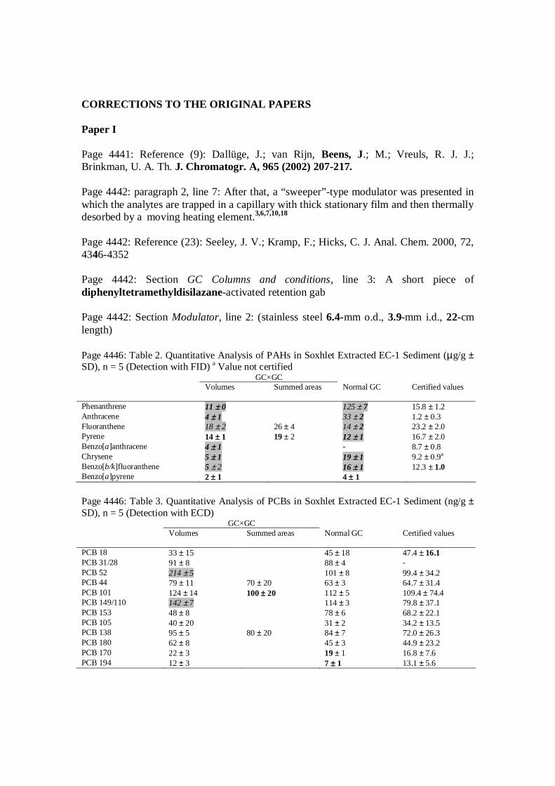
CORRECTIONS TO THE ORIGINAL PAPERS

Paper I

Page 4441: Reference (9): Dallüge, J.; van Rijn, Beens, J.; M.; Vreuls, R. J. J.;Brinkman, U. A. Th. J. Chromatogr. A, 965 (2002) 207-217.

Page 4442: paragraph 2, line 7: After that, a “sweeper”-type modulator was presented inwhich the analytes are trapped in a capillary with thick stationary film and then thermallydesorbed by a moving heating element.3,6,7,10,18

Page 4442: Reference (23): Seeley, J. V.; Kramp, F.; Hicks, C. J. Anal. Chem. 2000, 72,4346-4352

Page 4442: Section GC Columns and conditions, line 3: A short piece ofdiphenyltetramethyldisilazane-activated retention gab

Page 4442: Section Modulator, line 2: (stainless steel 6.4-mm o.d., 3.9-mm i.d., 22-cmlength)

Page 4446: Table 2. Quantitative Analysis of PAHs in Soxhlet Extracted EC-1 Sediment (µg/g ±SD), n = 5 (Detection with FID) a Value not certified

GC×GCVolumes Summed areas Normal GC Certified values

Phenanthrene 11 ± 0 125 ± 7 15.8 ± 1.2Anthracene 4 ± 1 33 ± 2 1.2 ± 0.3Fluoranthene 18 ± 2 26 ± 4 14 ± 2 23.2 ± 2.0Pyrene 14 ± 1 19 ± 2 12 ± 1 16.7 ± 2.0Benzo[a]anthracene 4 ± 1 - 8.7 ± 0.8Chrysene 5 ± 1 19 ± 1 9.2 ± 0.9a

Benzo[b/k]fluoranthene 5 ± 2 16 ± 1 12.3 ± 1.0Benzo[a]pyrene 2 ± 1 4 ± 1

Page 4446: Table 3. Quantitative Analysis of PCBs in Soxhlet Extracted EC-1 Sediment (ng/g ±SD), n = 5 (Detection with ECD)

GC×GCVolumes Summed areas Normal GC Certified values

PCB 18 33 ± 15 45 ± 18 47.4 ± 16.1PCB 31/28 91 ± 8 88 ± 4 -PCB 52 214 ± 5 101 ± 8 99.4 ± 34.2PCB 44 79 ± 11 70 ± 20 63 ± 3 64.7 ± 31.4PCB 101 124 ± 14 100 ± 20 112 ± 5 109.4 ± 74.4PCB 149/110 142 ± 7 114 ± 3 79.8 ± 37.1PCB 153 48 ± 8 78 ± 6 68.2 ± 22.1PCB 105 40 ± 20 31 ± 2 34.2 ± 13.5PCB 138 95 ± 5 80 ± 20 84 ± 7 72.0 ± 26.3PCB 180 62 ± 8 45 ± 3 44.9 ± 23.2PCB 170 22 ± 3 19 ± 1 16.8 ± 7.6PCB 194 12 ± 3 7 ± 1 13.1 ± 5.6

Paper II

Page 725: Introduction, line 4: The rapidity of the second separation step is achievedthrough use of a column that is shorter than the first column.

Page 728: Section Effect of modulation on peak widths and heights, line 1: Peak widthsfor modulated n-alkanes and PAHs at half height (2.35 ) were 70–100 ms.

Page 729: Section Mass conservation, 10: Phillips et al. [4] have reported

Paper III

Page 69: Right column, line 1: The turning took about 40 ms.

Paper IV

Page 253: Section Equipment, paragraph 2, line 6: The first column 20 m × 0.25 mm ×0.25 µm (HP-5MS).

Paper V

Page 238: Figure 3(a-b): The aldehyde overlapping with alloaromandrene should bedodecanal, not undecanal.

Page 240: Section Comparison of identification procedures, paragraph 2, line 11: In GC–MS analysis, the small peak of alloaromadendrene is overlapped by the peaks of alkanesor alkenes (not shown) in Fig. 3a and dodecanal. … more importantly, from more polardodecanal.

Paper VI

Page 229: Section Chemicals, line 1: Acetone, n-hexane, toluene, dichloromethane andethylacetate…

comprehensive two-dimensional gas chromatography ... · university of helsinki department of...

Documents