compliance averaging of soil contaminant concentration
TRANSCRIPT
Compliance Averaging of Soil Contaminant Concentration Data
under Ch. NR 720, Wis. Admin. Code
Wisconsin Department of Natural ResourcesP.O. Box 7921, Madison, WI 53707
dnr.wi.gov, search “brownfield”
DNR-RR-991 October 2015
!(!(
!(!(
!(
!( !(
!(
!(
!(
!(
!(
!(
!(
!(!(
!(
!(
!(
!(
!(
!( !(
!(
!(
!(
!( !(
!(
!(
!(
!(
!(
!( !(
!(
!(!(
!(
!( !(
!(
!( !(
!(
!(
!(
!(
!(
!(
!(
!(
!( !(
!(
!( !(
!(
!(
!(!(
!(!(
!(
!(
!(
!(
!(
!(
!(
!(!(
!(
!(
!(
!(
!(
!(
!(
!(
!(
2
2
2 1
1
2
22
1
1.71.5
2.8
2.12.6
1.41.11.81.61.41.92.11.8
2.3 1.3 1.6 2.1 2.2 1.1 1.2
1.72.12.22.11.8
0.2
0.8
0.5
1.91.71.9
1.3 1.2 1.5 1.3
2.72.4
1.6
2.6
2.2
3.1
1.8
1.3
1.51.20.90.83.6
2.1 3.7 1.4 1.6 3.5
1.2 1.8
1.6 1.3 3.2
0.90.8
1.22.72.9
0 1,000 2,000500 Feet
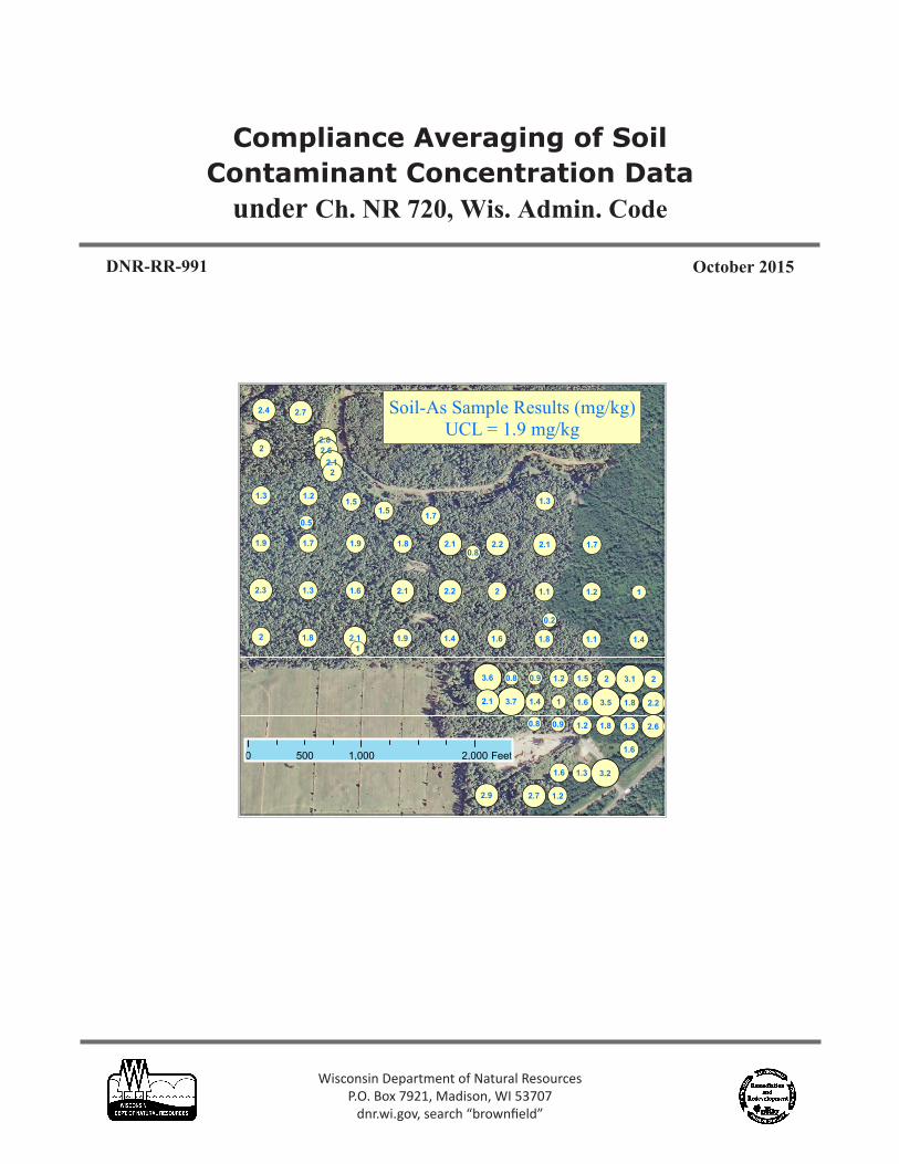
Soil-As Sample Results (mg/kg)UCL = 1.9 mg/kg

2RR-991
Table of Contents
I. Introduction ................................................................................................................. 3
A. Purpose of Guidance ................................................................................................ 3 B. Disclaimer, Contacts and Revisions ........................................................................ 3 C. Statistical Compliance Averaging - Is It Right for Your Site? ............................ 3 II. Compliance Averaging of Soil Contaminant Concentration Data ......................... 4
A. Overview ................................................................................................................... 4 B. Guidance Objective and Definition of Average ..................................................... 5 C. Using ProUCL Software from EPA ....................................................................... 5 III. Examples Illustrating Procedures Useful in Compliance Averaging .................. 6
Summary of Examples ................................................................................................... 6 Example 1: Simulation of a Mixture Population ........................................................ 7 Example 2: Separating a Mixture Population ........................................................... 12 Example 3: Misstep in UCL Calculation ................................................................... 14 Example 4: Straightforward Comparison between the DC RCL and the UCL .... 15 IV. Use of Background Threshold Values ................................................................... 16 V. Conclusion.................................................................................................................. 17 VI. References..................................................................................................................18
If you are reading a printed copy of this document and want to view the charts and images in a larger format go to the online PDF version of this document, at http://dnr.wi.gov/files/PDF/pubs/rr/RR991.pdf, and zoom in.

3DNR-RR-991
I. Introduction
A. Purpose of Guidance
The purpose of this document is to provide Department of Natural Resources (DNR) staff, responsible parties and other interested individuals with guidance on the application of administrative rules related to data averaging and the cleanup of soil contamination under NR 720, Wis. Admin. Code. This guidance document identifies a few key tools in the U.S. Environmental Protection Agency’s (EPA’s) ProUCL statistical software package for use in averaging soil data. Additional tools not covered here that may apply at a remediation site with multiple contaminants and sources can be found in EPA’s QA/G-9S publication (U.S. EPA, 2006). For more information contact Resty Pelayo, DNR, at [email protected] or (608) 267-3539.
B. Disclaimer, Contacts and Revisions
This document is intended solely as guidance and does not contain any mandatory requirements except where requirements found in statute or administrative rule are referenced. This guidance does not establish or affect legal rights or obligations and is not finally determinative of any of the issues addressed. This guidance does not create any rights enforceable by any party in litigation with the State of Wisconsin or the Department of Natural Resources. Any regulatory decisions made by the Department of Natural Resources in any matter addressed by this guidance will be made by applying the governing statutes and administrative rules to the relevant facts.
This guidance will be updated as needed. Questions, comments and concerns may be sent to: Judy Fassbender - RR/5, DNR, P.O. Box 7921, Madison, WI 53707. Phone: (608) 266-7278, E-mail: [email protected] [cc: [email protected]]
C. Statistical Compliance Averaging - Is It Right for Your Site?
Per NR 720.07(2)(b), Wis. Admin. Code, any alternative to point-to-point comparison to soil cleanup standards requires DNR approval. This document explains how one approvable alternative that involves – statistical averaging – may be developed to determine if applicable direct-contact soil cleanup standards have been met. Statistical averaging, as an alternative approach to determine compliance with soil cleanup standards, may not be appropriate at some sites. It is recommended that you contact your DNR project manager before deciding how to proceed with an averaging or any other alternative approach.
For practical and cost considerations, a minimum of 10 sample points from a single population is generally necessary before considering compliance averaging. Exploratory data analysis should be employed to gain insight into the data set collected and identify the best possible interpretation of data. For example, data from mixed populations (e.g., mixed background and hot spot data) requires processing to separate the different populations. Using averaging to avoid remediating hot spots is not acceptable. It is strongly recommended that a statistical averaging proposal be submitted early to DNR, long before submitting a case closure request (along with a NR 720 soil cleanup standard/report technical assistance fee) to avoid delays in the review and approval process.
4RR-991
A good understanding of statistics is necessary to complete the requisite data analysis for compliance averaging. For data analysis, DNR recommends using EPA’s ProUCL statistical software, which is available to DNR and consultants at no charge.
II. Compliance Averaging of Soil Contaminant Concentration Data
A. Overview
Numerical soil standards are termed soil residual contaminant levels (RCLs) in ch. NR 720, Wis. Admin. Code. Discrete point-to-point comparison is the primary mechanism to determine if a contaminant concentration in a soil sample exceeds the RCL. For direct-contact (DC) RCLs, however, there is an alternative to point-to-point comparison that DNR can approve: Compliance averaging.
The underlying concept is that, over time, the average is more representative of the concentration that would actually be contacted at the site. Hence, averaging, when done appropriately, canbe approved under NR 720.07(2)(b), Wis. Admin. Code as an alternative to straight point-to-point comparison to the DC RCL.
For the purpose of determining compliance with a numerical soil standard, compliance averaging for a particular contaminant will involve determining the 95% upper confidence limit for the mean (UCL) of the contaminant concentrations in soil samples. The true mean of a population is unknown but can be estimated from sampling. From the central limit theorem in statistics, the collection of random subsets of samples (each of size “n”) from a given population and the determination of means from each subset will provide for a normal distribution for the sample means, even if the given population’s distribution is not normal. However, estimating many sample means from several subsets of a population may not be possible due to the inherent large number of samples required to do so. Another procedure to estimate the true mean of a population is that when enough sample results are available, a confidence interval can be determined to provide a lower and upper limit centered about the sample mean for the sample results. For this procedure, the UCL is the upper limit of the confidence interval for the mean. The caveat, however, is that the confidence interval may not always include the true population mean. When taking subset after subset of samples from the population, and using each one separately to compute a 95 percent confidence interval, the expectation is that 95 percent of these intervals will include the true population mean. When only a single set of sample results is available, confirmation that the set belongs to the 5 percent group that may miss the true population mean is not available. Hence, it is necessary to assume that this is not the case. The aim of using the UCL is to provide a reasonable confidence that the true site average will not be underestimated. It is fundamentally important that the UCL be computed using a data set representing a single statistical soil population, and not from a mixture of populations.
Compliance averaging of soil concentrations may be appropriate where the contaminant is widespread, relatively consistent in concentrations and at levels close to the applicable RCL for that compound. This guidance includes several examples to illustrate important statistical exploratory concepts and to show the utility of a few tools available for calculating UCLs using EPA’s ProUCL software for the purpose of comparing the UCL with the DC RCL standard.

5DNR-RR-991
The procedure in determining compliance is generally straightforward if it can be established that there is a single population being represented by the observed concentrations. One key goal in any site investigation is the delineation of soil “hot spots” for remediation. As such, straightaway averaging of soil concentrations without considering the data distribution(s) may defeat that goal.
Averaging is not appropriate as the sole method for addressing sites where areas of significant soil contamination may exist. Unless a biased sampling plan directed toward a limited area ofconcern at the site is conducted, simple averaging cannot be relied on for addressing hot spots or source areas on a property. Summing the concentrations and then dividing by the number of samples to get the arithmetic mean may cause concentrations that are significantly higher than the applicable RCL to be “averaged away” by the more numerous low or non-detectable levels in the soil sample data set. Hence, this is not acceptable. Rather than simple averaging, many other States (e.g., New Jersey, 2012; Pennsylvania, 2013) allow the use of UCLs in their compliance averaging.
B. Guidance Objective and the Use of 95% Upper Confidence Limit for the Mean (UCL)
This guidance document provides general background information on the process and assumptions that need to be considered when statistically evaluating data. Although not intended to be a detailed discussion on statistical applications, this guidance identifies the use of a graphical Q-Q plot, outlier test and histogram plot to preliminarily categorize data before averaging is performed.
While “average” is generally understood to be the arithmetic mean of a list of numbers, the word average may also refer to the, median, mode, or some other central or typical value. In compliance averaging, the more-important statistic to use is the 95% upper confidence limit for the mean (95% UCL or simply, UCL).
The UCL provides a measure of uncertainty in the mean; it is not a measure of variability and should not be confused with a 95th percentile. The UCL is particularly dependent on the number of samples (or sampling size). As the sampling size increases, the difference between the UCL and the true mean decreases. The UCL provides a reasonable confidence that the true site average will not be underestimated when it is being compared to the RCL. The U.S. EPA’s Superfund program has used the UCL as the concentration term in point estimates of reasonable maximum exposure for human health risk assessment. In compliance averaging, the UCL will be used, simply to answer the question whether or not the UCL is greater than the DC RCL, to determine exceedance of the standard
An assumption in this guidance is that the individual responsible for analyzing the soil data has a good working knowledge of statistics and statistical applications, like knowing the use of and the difference between the 95% UCL and the 95th percentile statistics.
C. Using ProUCL Software from EPA
The critical first step in environmental data analyses is in determining the presence of multiple populations or outliers in the data set. Recognizing when two or more populations exist is

6RR-991
important because any calculated statistic will be meaningless if, for example, that statistic comes from unseparated “apples and berries” data. Likewise, recognizing outlying data is important because the statistics that include outliers will be distorted (often inflated) for the main dominant population. Further investigation of the outliers may be needed to determine the reasons for their occurrences (e.g., cross-contamination, contaminated locations). After separating out the different populations and having outlier-free subsets, the computation of the appropriate decision statistics (e.g., UCLs) for each identified population becomes a relatively straightforward task.
Given the technical scrutiny and range of options available in EPA’s ProUCL software, DNR recommends its use when statistically evaluating environmental data to determine if applicable soil cleanup standards have been met. It is available free to DNR and environmental professionals. The software, its documentation and training webinars can be found at: http://www2.epa.gov/land-research/proucl-software
The ProUCL tools described in this document help compute appropriate decision statistics, particularly the UCL. Other statistical tools and tests in ProUCL, besides the ones identified in this document, may also be acceptable but they have not been evaluated by DNR in detail and therefore are not discussed.
The focus of this document on compliance averaging is on calculating the UCL of the data set being evaluated, particularly pinpointing situations where averaging may be inappropriate. In general, the use of ProUCL to calculate the UCL requires at least 10 sample points, so if the site data set is smaller, the statistical approaches described here will likely not be usable. It is always a good idea to talk with your DNR project manager before deciding to use averaging at a site.
III. Examples Illustrating Procedures Useful in Compliance Averaging
Summary of Examples
The following pages include four examples with data sets. The statistical evaluation of the data sets is intended to illustrate the tools used in calculating UCLs so that it can be determined if the applicable direct contact RCL has been met. The procedures in the examples, if proposed for use at a site, are approvable as an alternative approach in NR 720.07(2) (b), Wis. Admin. Code.
• Example 1 simulates a mixture of data composed of random samples from two normal populations (“A” and “B”) having different means. When graphed using the normal probability plot or ProUCL’s quantile-quantile (Q-Q) plot tool, the mixture is depicted by 2 distinguishable straight-line segments, with A’s data falling nicely into one line, separable from B’s data falling in another.
• Examples 2 and 3 have actual site data where the Q-Q plot, outlier test and histogram chart are used in resolving the data sets as composed of subsets of several populations.
• Example 4 shows a straightforward RCL-UCL comparison. It is first established that the data set comes from a single population, and then the UCL is determined. If the UCL does not exceed the RCL, then that data set (even if there were point exceedances) meets the soil standard.

7DNR-RR-991
Example 1: Simulation of a Mixture Population
For this simulation, we assume perfect knowledge for 2 normal populations (“A” and “B”) with different true means and standard deviations. Population A has a true population mean (u) of 8
and a population standard deviation (sd) of 2. Population B has u=20 and sd=8. Schilling et al. [2002] identified several criteria for when data from 2 normal populations are separable. Our assumed populations qualify by having their true means (8 and 20, respectively) separated by at least the sum of their standard deviations (2+8=10). So when we have enough samples from both populations, we will expect two separate bell curves when we plot the histogram of their mixed data. In Example 1, we simulate the case where we have fewer samples from B (the population with the larger mean). This may more often be the scenario in many real site situations where because the contamination is small volumetrically and areally, fewer samples are collected in those areas relative to the uncontaminated area of the site. In Example 1, we create a mixture of the data from both populations, but with relatively fewer B samples so as not to easily see two bell curves.
������������
���������� �
������������
u �����sd ���
������������
���������� �
������������
u ������sd ���
�������� �
����� ��
���������
u ���������������������� � ��
sd ��������� � � ����� � �
������������ ������������ ����� ����� �
� �� �� �� �� �� ��
� � �� �� �� � ��
� � �� �� �� � ��
� � �� �� �� � ��
� � �� �� �� � ��
� �� �� �� �� �� ��
� � �� � �� � ��
� �� �� �� �� �� ��
� � �� � ��
�� � �� � ��
�� � �� � ��
�� � �� � ��
�� � �� � ��
�� � �� � ��
�� � �� � ��
�� � �� � ��
�� � �� � ��
�� � �� � ��
�� � �� � ��
�� � �� � ��
�� �� �� �� ��
�� � �� � ��
�� � �� � ��
�� � �� � ��
�� � �� � ��
�� � �� � ��
�� � �� � ��
�� � �� � ��
�� � �� � ��
�� � �� � ��
�� �� ��
�� �� ��
�� �� ��
�� �� ��
�� �� ��
�� �� ��
�� � ��
�� �� ��
��� � �� � �� � ��
���� �� �� �� �� �� ��
����������� � �� �� �� �� ��
��������� ��� � � �� � �� � ��
��������������������������� ������������������������������������������������
������������������������������u���������������������������������sd�����������������������u�������sd������������������������������������������� ���������������������������������������������������������
���������������������������� ������ �������� ���������������������������������������� �������������������������� ������ �������� ������������� �������������������������� �������������������������� ���������������
�������� ������������������������������������ ������������������������������������������������������������ ����������������������������������������������
������ �������������������������� ���������������������������������������������������������������������������� �������������������������������������������������������������������� ���� ��������� �������������������������������������������������� � �������������������������������� ����������������������������������������������������
���������������� ����������������������������� ������������������������������������� ������������������������������������������������������������������������� �������������� ���� ��������������������������������������������������� ����������������������� ��������������� ����������������������������������� � ���������������� � �� ����������������������������������������� ��������� ������������������������������������������������������������������������������
������������������������������������������������� �����������������������������������������������������������������������������������������������������
������������������������������������������
���������������������
The data table in Box 1 for Example 1 shows our randomly-generated sample values from Population A (sample size n: 30; sample mean x: 7.38), Population B (n: 8; x: 19.86) and the Mixture A and B (n: 38; x: 10.01). The first thing to note is that with the mixture population, we have calculated a mixture sample mean ( x: 10.01), a numerically “in-between” statistic that is not particularly relevant to A (with true mean u = 8) nor B (u = 20).

8RR-991
The question is: Once mixed, is there a statistical tool to distinguish “A” samples from “B” samples? The answer is: Yes, and the best distinguishing tool is to render a quantile-quantile or Q-Q plot for the mixed data. Most of the data points from “A” will fall along a line, and similarly, most of the data points from “B” will fall along another line segment in the Q-Q plot. The right panel of Box 2 for Example 1 has the Q-Q plot for the mixed data. In this Q-Q plot, the whole range of the mixture data set is displayed, arranged from the lowest to highest value along the vertical y-axis. The Q-Q plot’s horizontal x-axis has the theoretical normal quantile values. Having the larger mean, the “B” data set plots higher (along the “High” Data Line), separate from the “A” data (“Low” Data Line).
Q-Q Plot. The Q-Q plot is also known as the normal probability plot. This graphical tool is used in many statistical data analyses to gain insight into data sets collected in the different fields of biology, medicine, geochemical prospecting and environmental studies. The probability plot approach has been used in geochemical prospecting for over 50 years [e.g., see Carranza, 2008, for published references dating back to 1959] to identify outliers and geochemical anomalies, to examine potential multiple populations, and to define the breaks or inflection points at which to subdivide the data set into subsets representing those populations. The apparent jumps and breaks in the Q-Q plot suggest the presence of multiple statistical populations [e.g., Fowlkes, 1979]. The normal probability plot or its equivalent cumulative probability plot has been used to separate
������������������������������� � ����������������������������������������������
����� � �������������������������������������������������������������������������������������������������������� �
���������������
��������������
�������� � ��������������������������������������������������������������������������������������������������� ������������������������������������������������������������ � ����������������������������������
������������������������������������ �����������������������������������������������������������������������������������������������������
����������������������������������� ����������������������������������� �������������������������������������������������������������������������������������������������
��� �
����������������������������������������������������
������������������
����

9DNR-RR-991
background levels from contaminated levels [e.g., Fleischhauer and Korte, 1990]. The inflection points on the Q-Q graph indicate an interpretable breakdown of the distribution into separable populations with different means [e.g., Singh et al., 1994]. However, the identification of the exact break points (or threshold values for the different populations) in a Q-Q plot is highly subjective, requires experience, and so is not a trivial task. Historical and theoretical reviews of decomposing finite mixture distributions can be found in Holgersson and Jorner [1978], Sinclair [1991] and Everitt [1996]. For this guidance, we limit our discussion to the graphical and visual fit of straight lines to Q-Q plot segments. Rather than delve into advanced routines (e.g., determining the intersection for 2 line segments or minimizing the kurtosis for each population), the approach here will be more towards visually inspecting inflection points when picking a potential threshold value that separates one population from another. In many practical applications, this visual approach may suffice in determining statistically valid conclusions.
In ProUCL’s Graph, we rendered the Q-Q plot of the mixture A and B data to show that with their different slopes, the “high” and “low” data lines are distinguishable and that their dissimilarity can be the basis for their separation. Upon close inspection of the Q-Q plot for the mixture, it seems apparent that the threshold value (on the y-axis) separating A and B is around 12, such that values less than 12 may be categorized as belonging to “A,” while values larger may be categorized as “B” sample points. This simple procedure of visually picking 12 did not resolve the categorization of all the data. Out of B’s original 8 sample points (see Box 1 for Example 1), there are now after mixing only 7 that we can resolve as “B” results because B’s lowest value (9.03) was less than 12. Nevertheless, we have accomplished most of the “un-mixing,” such that when we proceed to calculate the statistics for two (2) separate subsets (below-12 and above-12), we will get more meaningful unmixed statistics for the 2 separate populations.
Outlier Tests. Another tool that may be useful in separating A from B is the outlier tests under ProUCL’s “Statistical Tests.” The outlier test is particularly helpful when the mixture data set is dominated by samples from a main population with only a few data from another – which aptly describes our mixture A and B data. The result from the outlier test may help corroborate the result from our analysis using the Q-Q plot. One important consideration in testing for outliers is that it should be performed on raw data, as the cleanup decision needs to be made based upon concentration values in the raw scale and not in the log-scale. ProUCL’s outlier test tool applies 1 of 2 “classical” outlier tests, either the Rosner’s or Dixon’s test, depending on how many data points are present. (“Modern” robust outlier tests exist, but they are not tools in ProUCL.)
ProUCL carries out the Rosner’s test when the sample size n ≥ 25; otherwise, ProUCL applies the Dixon’s test. For the mixture A and B data (n: 38), the Rosner’s outlier test was performed. The outliers identified by the test are in Box 3 for Example 1. The Rosner’s test can be used to identify up to 10 outliers. The test procedure is described more fully in Gilbert [1987]. In ProUCL, the number of suspected outliers is specified before the Rosner’s test is run. Specifying how many outliers are suspected is an important step in the Rosner’s test. Counting suspected outliers from the Q-Q plot can help in initially deciding how many there are. If more than 10 are suspected, it is procedurally possible to delete so as to exclude the most obvious outlying data to reduce to 10 or less the number of suspected points subjected to Rosner’s test. For a suspected extreme outlier, a Rosner test statistic is computed by getting the difference between

10RR-991
the outlier and sample mean and dividing the difference by the sample standard deviation. If this test statistic is greater than a certain critical value, then the conclusion is that the extreme outlier is indeed an outlier; otherwise, it is not. However, the presence of intermediate (less extreme) outlier(s) can inflate the sample standard deviation (divisor in the test statistic), making the test-value statistic small. This, in turn, can make the test inconclusive about the extreme outlier. In other words, the presence of other outliers in between the extreme value and the main population may “mask” the fact that the extreme value is an outlier. To minimize masking, the Rosner’s test proceeds by excluding the extreme value and computing a new test statistic for the next extreme outlier. The procedure is repeated for how many suspected outliers we initially specified.
The Rosner’s test on mixture A and B identified the 6 largest values as outliers (Box 3). How the test identified the outliers requires some description. For the first extreme observation (27.15), its test-statistic value (2.87) is less than the critical value (either 3.01 or 3.36), so initially we cannot conclude it as an outlier. Had we specified only 1 (rather than 10) suspected outlier before the test is run, the test would not have identified this extreme point as an outlier. In the next iteration, the program discards the 1st extreme point and calculates a 2nd test value for the 2nd extreme point (26.05). The 2nd test value (3.05) is greater than the 5% critical value (3.), but is less than the 1% critical value (3.34). So had we specified only 2 suspected outliers, the Rosner’s test at 5% significance would have identified the 2nd extreme value (26.05) as an outlier, but the test at 1% would not. Upon proceeding and by the 6th test statistic, it becomes apparent why the first
���������������������������������� ��� ���������� ����������� ������������ ������������������� ���������������������� ������������������������������������� ������������� ��������������
� �������������������� �������������������������������������������� ����������������� �������������� ����������������� �����������������������
������ ������������������������������������������
���������������������������� ������� �������������������
������������������������������������������������������������������� ������������������������������������� ���������������������������
���� ������������������������������������ ������ �� ��������������� ������������������������ ������� ��� ������������������������������������������ ��� ������������� ������������������
����������������� �
� ����������� �����
������������������������������������������������������
���������������� ���

11DNR-RR-991
few more-extreme data points (27.15, 26.05, …, 21.36) had low test-value statistics. The sample standard deviations for their test values were inflated because there were other outliers remaining in the data set. Those intermediate outliers had obscured (or masked) the presence of the more extreme outlier. By the 7th test and on, the Rosner’s test did not result in any more outliers being identified. The Rosner’s test did not identify the 7th suspected point (14.62) as an outlier, even though based on the Q-Q plot, it is a point to be included in the “B” (not “A”) subset. When a value is in close proximity to the inflection point between 2 populations, it is not uncommon for a data point to be incorrectly classified. This is typically not a major concern because the more extreme data points have already been identified as outliers. So even though the outlier test did not corroborate all 7 values from the Q-Q plot as non-“A” data (nor the 8 original simulation B sample data), what is important in the outlier test result is that it identified the presence of values not belonging to A, the main population represented by the samples.
Histogram. A third tool that can help distinguish populations is by graphing the data histogram. The rendered histogram for the mixture A and B is shown in Box 4 for Example 1. ProUCL allows for either decreasing or increasing the number of categories or bins for the histogram. Generally, the utility of the histogram may be limited because of the number of samples (typically, too few for either of the populations), the proximity between the population means or the unequal standard deviations for the populations. How the histogram is rendered is affected by the number of bins. With the sample histogram we can only try to capture the shape of the population distribution, so with too few bins, the shape is lost. And then with too many bins, the shape is likewise lost. Nevertheless, the histogram’s practical use is that it should illustrate the conclusions derived from the Q-Q plot and the outlier test.
�����������������������������
��������� ���������������������������������������� ��������������������������������� ���������������������������������������������������������������������������������������������������������������������������� ��������������������������������������������������� ������������������������������������������������������������������������������� ���������������������������� ������ �������������
� ������������������������ �� ����������� ������������
�������������������������������������������� � ��������
���������������������

12RR-991
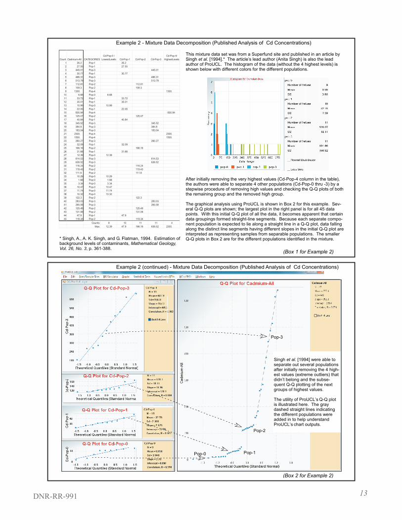
Example 2: Separating a Mixture Population
One of the inherent assumptions required to compute the UCL for the mean is that the data set under consideration originated from a single statistical population [EPA, 2013, ProUCL Version 5.0.00 Technical Guide, p. 8]. To avoid calculating statistics that may be meaningless, it is important to be able to recognize if multiple populations may be present in the soil data set we have. Correctly characterizing the distribution of the sample data set provides for robust statistics for use in any site decision. A normally distributed data set with a few high observations– such as those expected from hot spots– can be incorrectly modeled by the lognormal distribution with the outliers conveniently hidden by the lognormal assumption. An incorrect assumption on the data distribution, either because of the presence of outliers or the fact that the data set is from two or more populations, may result in misleading statistics. Data from a site investigation generally consist of samples from clean (uncontaminated) and contaminated parts of the site. As such, it is reasonable to think of the data set as a mixture of (at least) 2 populations with the idea of separating them out first before any statistical analysis. Population partitioning is not a trivial exercise, so a published example is included here to illustrate what steps may be involved.
Example 2 has a mixture data set from a Superfund site where, even after the removal of the most obvious extreme outliers (column Cd-Pop-4), not just 2, but 4 component populations (with varying degrees of contamination levels) have been identified and separated by a partitioning technique developed by Singh et al. [1994]. The histogram in Box 1 for Example 2 displays the different identified populations; each population is represented by a unique color in the histogram. It is apparent from the colors that the spread or width of each population varies, highlighting why the histogram may not be the best initial tool to separate out the populations. A bin width of 50 may be suitable for the very wide data shown in green (Pop-3), but it will then lump together the 2 narrower populations with the lowest means in dark blue (Pop-0) and red (Pop-1).
The Q-Q plot for all the data is shown in the right panel of Box 2 for Example 2. This initial Q-Q plot can generally provide an idea about the number of populations present. Singh et al.’s [1994] decomposition of the data relied heavily on the Q-Q plot, and the gaps and straight line segments identifiable in the Q-Q plot. Each line segment in the initial Q-Q plot represents data from a separable normal population. The subset of data falling along a line segment is considered a component population and its separate Q-Q plot constructed. These “component” Q-Q plots are shown in the left panels. An interesting aspect of this analysis is that the lowest identified component can be thought of as coming from background. Hence, the decomposition procedure can be followed for estimating the statistics for site-specific background level at remediation sites, specifically in identifying a background threshold value (BTV). Once determined, any concentration greater than the BTV can be concluded as exceeding background.
13DNR-RR-991
���������������������������������������� �������� ������������� �� ����������� ����������������������������������������������� ������ ���������������������������������� ������������������������������������������������������������������ ������������������� ����������������������� ����������� ��
������� ������������� �������������������������� ������������ �� ��������������������������������������������������������������� ��� ����������������������������������������������� ��������������� ������ �������������������������������� � ��������� �������������������������
�������������� ��������� ������ �������� �� ����������������������������������������������������� �������������������� ������������� ������������������������ ���������������� ������������������������������������������������ ������������ ����������� ��������������������� ������� ������������������������������ � ����������� ���������������������� ��������������� ��� ����������������������� ���� ����������� ���� ������� ������� ��������� ���������� ������ ������������������� �������������������� �� ���������������������������������� �������������������������� �������������������������� ����������� ����� �������� ����������������� ���������������� ����� ����������� ������������������ ���
������� ������������� ���� � ������������������������������� ��������������������
������������������������������������ ������������� ���������� �� � � ������ ���
�� � ���������� ���������
����������
���������� ������� ������� �������
���������
������������
� ���� ����� ����
� ����� ����� �����
� ������ ����� ������
� ����� ����� �����
� ������ ����� ������
� ������ ����� ������
� ������ ����� ������
� ����� ����� �����
� ����� ����� �����
�� ���� ����� ����
�� ����� ����� �����
�� ����� ����� �����
�� ����� ����� �����
�� ����� ����� �����
�� ������ ����� ������
�� ������ ����� ������
�� ����� ����� �����
�� ������ ����� ������
�� ����� ����� �����
�� ������ ����� ������
�� ����� ����� �����
�� ����� ����� �����
�� ������ ����� ������
�� ����� ����� �����
�� ������ ����� ������
�� ����� ����� �����
�� ����� ����� �����
�� ������ ����� ������
�� ������ ����� ������
�� ������ ����� ������
�� ������ ����� ������
�� ����� ����� �����
�� ����� ����� �����
�� ���� ����� ����
�� ���� ����� ����
�� ����� ����� �����
�� ����� ����� �����
�� ����� ����� �����
�� ����� ����� �����
�� ������ ����� ������
�� ������ ����� ������
�� ������ ����� ������
�� ������ ����� ������
�� ���� ����� ����
�� ������ ����� ������
�� ��� � �� �� �� �
���� ����� ���� ������ ������ �����
�������������������
�����
�����
����������
�������������������� �������������������������������������������������������������������������������������������������������������������������������������� � ��������������������������������������������
������������������������ � �������������������������������������������������������������������������������������� �������������������������������������������������
����������������������������������������������������������������������������������������
���������������������

14RR-991
Example 3: Misstep in UCL Calculation
Soil-PAH (polycyclic aromatic hydrocarbon) samples were collected for direct-contact evaluations (sample depths between 0 and 4 feet) at an industrial site that was a bulk petroleum storage terminal for over 100 years. Today, it is no longer a bulk terminal, and several non-residential buildings and vacant lots are now situated at this redeveloped site. It was found that BaP (benzo[a]pyrene) was the most-frequently encountered PAH to exceed its direct-contact soil residual contaminant level (RCL) of 0.211 mg/kg allowed at industrial sites. The soil-BaP data are tabulated in Example 3.
The table did not include some data (empty cells) as a decision regarding them (excavation) was already in place. The table shows that over half of the BaP data are “NDs.” (In a ProUCL input table, “ND” means entering the lab detection limit under the BaP column followed by a “0” flag in the d_BaP column.) Hence at the outset, based on the frequency of NDs, there is already an indication of at least 2 populations. Example 3 is provided here to show how an inappropriate UCL estimate can be misleading.
The 4 highest concentrations (shown in red in the table) are greater than BaP’s RCL of 0.211 mg/kg. Without regard to the presence of multiple populations, plugging the data into ProUCL
������������������������������ �������
��������������������������������������������
�
��������������������������������������������������������������
�
�������������
���������������������������
������������������������� ��
���������������������
��� ����������������������� �� ������������������������ ����������������������������������������������� ���������������� ��������������������������������������������������
�������������� �����
�������������������������������������� �������� ���� ��������������������������������� ���������������������������� ������������ ��������������������� ������������������ ������������������������������������������������������ �� ���������������������� �� �������������������������������������������������������������������������������������������������������������������� ����������������������� ��������������������������������� ��������������������������������� ������������������������������������������������������������������������������ ����� ������������������
�����������������������������������������������������������������������������������������������������������������������������������������
������
�����
����� ��� �����
� ����� �
� ����� �
� ������ �
� ������ �
� ������ �
� ������ �
� ����� �
� ������ �
� ������ �
�� ����� �
�� ������ �
�� ������ �
�� ����� �
�� ������ �
�� ����� �
�� ������ �
�� ������ �
�� ����� �
�� ������ �
�� ����� �
�� ������ �
��
�� ������ �
�� ����� �
��
�� ������ �
�� ������ �
�� ������ �
�� ������ �
�� ������ �
�� ������ �
��
�� ����� �
�� ����� �
�� ������ �
�� ������ �
�� ������ �
�� ������ �
��
��
�� ������ �
�� ������ �
�� ������ �
�� ������ �
�� ������ �
�� ������ �
�� ������ �
��
�� ������ �
����

15DNR-RR-991
would result in UCL estimates that are less than 0.2 mg/kg. However, the Q-Q plot for the data shows the “disconnect” between the low values and the high values; the latter as a group has a distinctly steeper slope.
The Q-Q plot strongly suggests that the high values should not be grouped together with the low values. In addition to the Q-Q plot, because the majority of the data is “ND”, it is fairly easy to show that the 4 highest values (all >0.211 mg/kg RCL) are outliers. Hence, the conclusion after our statistical analysis is that more scrutiny is needed where the 4 highest levels are located. They are RCL exceedances that cannot be included with the main population that are less than the RCL.
In this example, we illustrate that in many practical applications, it is not necessary that we proceed to determine the UCLs for every statistical population. To make a decision about averaging and RCL exceedances, it may likely suffice to show that concentrations exceeding the RCL standard are not from the same statistical population as those not exceeding the RCL.
Example 4: Straightforward Comparison between the DC RCL and the UCL
With this last example, Example 4 (on p. 16), we illustrate how it is possible that some data may exceed the DC RCL, but that no further remediation may be necessary because the UCL for the data set did not exceed the RCL. The prerequisites to such comparison include: 1.) Establishing statistically that the UCL was estimated for a dataset coming from a single population, and 2.) Estimating the UCL with no outliers present. When these prerequisites are met, then the UCL (rather than individual point concentrations) can be directly compared to the RCL. When the UCL does not exceed the RCL, then the RCL is met. Outliers exceeding the RCL, or other data from another population whose UCL exceeded the RCL, will still need to be addressed either with further investigation or remediation.
The data set for Example 4 has 13 point concentrations, with the highest 3 greater than the RCL (10 mg/kg) for contaminant X. The Q-Q plot shows that all 13 points fall nicely along a single straight line. Because the data set has less than 25 points, the Dixon’s (not Rosner’s) outlier test was used to determine whether outliers were present. The outlier test yielded no outliers in the dataset. So all of the data were then used to calculate the UCL. The resulting UCL was less than the RCL (10). This means that even though 3 individual points were above the RCL, no further work at the site is necessary because the UCL did not exceed the RCL standard.

16RR-991
IV. Use of Background Threshold Values
Another option for statistically evaluating site data is to initially establish a background threshold value (BTV) for the contaminant of concern. This option may be appropriate when the contaminant is either naturally occurring or perhaps attributable to atmospheric deposition. This typically includes metals and PAHs. ProUCL provides several tools to analyze for the background threshold value (BTV). The BTV is typically set by the upper tolerance limit of the 90th or 95th percentile, or even the maximum of an acceptable background reference dataset. So the BTV is a statistic of higher-order than the UCL for the mean.
To illustrate what a BTV is compared to a UCL, we go back to the population partitioning shown in Example 2. After population partitioning, the background subset can be separated from other populations. In Example 2, the column “Cd-Pop-0” has the subset comprising the background data set. Its maximum concentration (12.39) is the BTV. The UCL value (11) is less than BTV. (Because there are less than 10 data points in Cd-Pop-0, running ProUCL to determine the UCL for the data set will give a warning about the small sample size. The UCL of 11 is calculated assuming the normal t-distribution for the data points.) Utilizing population partitioning to establish site-specific BTV can be a useful option at sites where the threshold level, like for the naturally-occurring background concentrations, may be set as the soil cleanup standard.
������� ���� � ��
�������� ������������������ �������
������ ������� ��� �����������
����������� ��� �� �
�������������� ����������� ������� �������� � ����������������� �������
�� ������� ��������� ����������� ������� ����������
������� ������� ����� ���������
� ����������� ������������ ���� �����������
������ ������������������ ���������� ������ �����������
��������� ����������������� ����������� ���������������������������� �����������
��������������
��������������������������� ���������� ��������� ��� ��������
����������������������������� ����������� ���������������������������� �����������
�������������������� ����������� ������������������������������� �����������
����������� ��������������������� �����������
�������������������� �������� �� ���������
��������������� �������� ��
� � �������������� � � ������������������� �����������
������������� ������
����������������� �����������
���������������������������������������� ������������������������������������������������������������������������������
��������������������������������������������������������������������������������������� ���
������ ����������������������������������
�
�������������������������
���������������������������������������������
������� ��������������
� ��
��
� ���
� �
� �
� ���
� ��
����
���
�� ���
�� ��
� ��
�� ��
�������������������������������������������������������������������������������������������������������������������������������������������������������������� ���� ��
��������������������������������������������� ��������������������������������������������������������������������������������������������������������������������������������������������������������
������������������������������������������������������������������������������������������������������������������������������������������������������������������������������������������������������������������������������������������������������������������������������������������������������
���������������������������������������������������������������������������������������������������������������������������������������������������������������
������������������ �������������� ���
�������� ����������������
�������������������������
������������������������
������������������������
���������������������
��� �������������������� ����������������������������������
���������������������
������������ ��������������������������������
������������ �������������������������������
����������� �������������������������������
����������� �������������������������������
����������� ��������������������������������
����������� ��������������������������������
��������������������� ����������������������������������
��
��
�

17DNR-RR-991
After a statewide background sampling in Wisconsin, a different method was used in establishing the statewide surficial soil-arsenic BTV. The statewide sampling was designed so as to exclude obvious anthropogenic influences to achieve values that are as close as possible to a natural baseline while recognizing that few areas are pristine. The methodology for establishing a BTV is contained in the ProUCL Technical Guide when NDs (not detected) are plentiful in the background dataset. The USGS [Stensvold, 2012] had used ProUCL in evaluating the data during the development of a report to determine the distribution and variation of surficial soil-arsenic in Wisconsin. Nearly one-third (211 out of 664 sample results) of the soil-arsenic samples were NDs (< 1 mg/kg). The data set was evaluated for outliers and the data points identified as outliers were removed so as not to bias the higher-order statistics. The DNR Remediation and Redevelopment (RR) program defined the statewide BTV for soil-arsenic as the highest value from the dataset once the outliers have been removed. The outlier-free maximum value can then be categorically accepted as not exceeding background. The guidance document (RR-940) explaining how the statewide BTV for arsenic was established is available at: http://dnr.wi.gov/files/PDF/pubs/rr/RR940.pdf. It has a table with the UCL (2.4 mg/kg) and BTV (8 mg/kg) for the outlier-free statewide soil-As background data set.
The statewide BTV definition used for arsenic (i.e., maximum without outliers) was extended to the other metals included in the USGS report. These statewide BTVs for arsenic and other metals are incorporated in the spreadsheet of RCLs available from the RR program. Since both RCLs and BTVs are available in the same spreadsheet, it is worth mentioning how they need to be applied when it comes to site UCLs. In practical application, a site’s UCL can be compared to an RCL; however, that UCL should not be compared to the statewide BTV.
It is re-emphasized here that the UCL is not the same as the BTV. The comparison of a 95% UCL of one population with a 95th percentile or the maximum of another population (as the BTV can be defined) cannot be considered fair and reasonable as these limits (UCL and BTV) represent different parameters [U.S. EPA, 2013, p. 20].
A site-wide UCL for a contaminant is not needed for comparison to its respective statewide BTV. Each individual data point from the site should be compared to the statewide BTV to determine if that data point exceeds background or not. To the degree that an individual point is less than the BTV, that sample result would be considered background.
V. Conclusion
The use of statistics to evaluate environmental data requires a good working knowledge of statistics. Specialized assistance may be needed to appropriately use statistical averaging to comply with NR 720, Wis. Admin. Code.
The averaging approach outlined in this guidance document may be useful in some situations, where data is plentiful. However many sites will typically have insufficient data for statistical analysis to be used, and it will simply be unnecessary at many more sites where a reasonable and environmentally sound remedy can be identified through other methods.
For other statistical procedures that may be applicable and approvable at different stages of the remediation process, it is strongly recommended that the Responsible Party discuss potential

18RR-991
options with the DNR Project Manager, before taking action, to help ensure the selected method is appropriate for the data set being evaluated. For more information contact Resty Pelayo at [email protected] or (608) 267-3539.
VI. References
Carranza, E. J. M., Geochemical Anomaly and Mineral Prospectivity Mapping in GIS, Handbook of Exploration and Environmental Geochemistry, Vol. 11 (M. Hale, Editor), The Netherlands: Elsevier B.V., 351 pp., 2009.
Everitt, B. S., An introduction to finite mixture distributions, Statistical Methods in Medical Research, Vol. 5, No.2, p. 107-127, 1996.
Fleischhauer, H. L., and N. E. Korte, Formulation of cleanup standards for trace elements with probability plots, Environmental Management. Vol. 14, No. 1, p. 95-105, 1990.
Fowlkes, E. B., Some methods for studying the mixture of two normal (lognormal) distributions, Journal of the American Statistical Association, Vol. 74, No. 367, p. 561-575, 1979.
Gilbert, R. O., Statistical Methods for Environmental Pollution Monitoring, New York: Van Nostrand Reinhold, 320 pp., 1987.
Holgersson, M., and U. Jorner, Decomposition of a mixture into normal components: A Review, International Journal of Bio-Medical Computing , Vol. 9, No. 5, p. 367-392, 1978.
New Jersey Department of Environmental Protection, Site Remediation Program, Technical Guidance for the Attainment of Remediation Standards and Site-Specific Criteria, 48 pp., 2012. Retrieved May 1, 2015, from: http://www.nj.gov/dep/srp/guidance/srra/attainment_compliance.pdf
Pennsylvania Department of Environmental Protection, Land Recycling Program Technical Guidance Manual, Section IV - General Guidance, 143 pp., 2002. Retrieved May 1, 2015 from: http://www.elibrary.dep.state.pa.us/dsweb/Get/Document-98303/253-0300-100%20Section%20IV.pdf
Schilling, M. F., A. E. Watkins, and W. Watkins, Is human height bimodal?, The American Statistician, August 2002, Vol. 56, No. 3, p. 223-229, 2002.
Sinclair, A. J., A fundamental approach to threshold estimation in exploration geochemistry: Probability plots revisited, Journal of Geochemical Exploration, Vol. 41, p. 1-22, 1991.
Singh, A., A. K. Singh, and G. Flatman, Estimation of background levels of contaminants. Mathematical Geology, Vol. 26, No. 3, p. 361-388, 1994.
Stensvold, K. A., Distribution and variation of arsenic in Wisconsin surface soils, with data on other trace elements: U.S. Geological Survey Scientific Investigations Report 2011–5202, 41 pp., 1 app., 2012.
U.S. EPA, Data Quality Assessment: Statistical Methods for Practitioners, EPA QA/G-9S, U.S. Environmental Protection Agency Office of Environmental Information, Washington, DC, EPA/240/B-06/003, 198 pp., 2006.
U.S. EPA, ProUCL Version 5.0.00 Technical Guide, Statistical Software for Environmental Applications for Data Sets with and without Nondetect Observations, U.S. Environmental Protection Agency Office of Research and Development,Washington, DC, EPA/600/R-07/041, 273 pp., 2013.