complexity theory - lecture 24: circuits and parallel ... · circuits and parallel computation...

Circuits and Parallel Computation

Complexity TheoryCircuits and Parallel Computation

Daniel Borchmann, Markus Krötzsch

Computational Logic

2016-01-19

cba

cba 2015 Daniel Borchmann, Markus Krötzsch Complexity Theory 2016-01-19 #1

http://lat.inf.tu-dresden.de/~borch

http://korrekt.org/


http://korrekt.org/

https://ddll.inf.tu-dresden.de/web/Complexity_Theory_(WS2015)

Circuits and Parallel Computation Review

Review



http://korrekt.org/


Circuits and Parallel Computation Modelling Parallelism With Circuits

Modelling Parallelism With Circuits



http://korrekt.org/



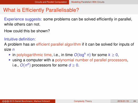
What is Efficiently Parallelisable?

Experience suggests: some problems can be solved efficiently in parallel,while others can not.

How could this be shown?

Intuitive definition:A problem has an efficient parallel algorithm if it can be solved for inputs ofsize n

in polylogarithmic time, i.e., in time O(logk n) for some k ≥ 0,using a computer with a polynomial number of parallel processors,i.e., O(nd) processors for some d ≥ 0.

Note: Using O(nd) processors efficiently requires a massively parallelalgorithm. However, one could always use fewer processors (each takingon more work), possibly leading to a proportional increase in time.

The hard bit in parallelisation is to utilise many processors effectively –reducing to fewer processors is easy.



http://korrekt.org/



Modelling Parallel Computation

What kind of “parallel computer” do we mean here?

(1) How do processors communicate?

(2) What can a processor do in one step?

(3) How are processors synchronized?

Detailed answer: define Parallel Random Access Machine (PRAM)

Our answer:Details are not critical as long as we can make some general assumptions:

(1) Every processor can send a message to any other processor inO(log n) time

(2) In one step, each processors can perform one Boolean operation on“a few” bits, say O(log n)

(3) Processor steps are synched with a global clock



http://korrekt.org/



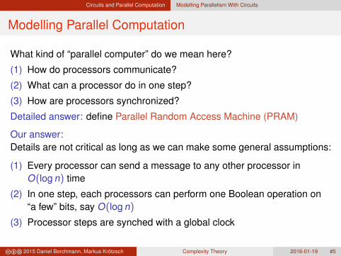
Modelling Parallel Computation in Circuits

Simple PRAM computations can be mapped to Boolean circuits(with some extra circuitry for executing more operations or for modellingmessage passing)

Circuits as models for parallel computation:

circuit gates can operate in parallel – they only depend on their inputs

the time needed to evaluate a circuit depends on its depth, not size(depth = longest distance from an input to an output node)



http://korrekt.org/



Example: Generalised AND

The function that tests if all inputs are 1 can be encoded by combiningbinary AND gates:

. . .

. . .

. . .

. . .

(n/2 gates)

(n/4 gates)

. . .

x1 x2 x3 x4 x5 xn. . .

size: 2n − 1

depth: log2 n



http://korrekt.org/



Small-Depth Circuits

Small depth = short (parallel) time

However: Every Boolean function can be computed by depth O(log n)circuits using O(n2n) gates (exercise)

Hence, to capture “efficient parallel computation”, we also restrict the size:

Definition 18.1

For k ≥ 0, we define NCk to be the class of all problems that can besolved by a circuit family C = C1,C2,C3, . . . such that

the depth of Cn is bounded by O(logk n), and

there is some d ≥ 0 so that the size of Cn is bounded by O(nd)(in other words: C ∈ P/poly).

(NC is for “Nick’s class”, named in honour of Nicholas Pippenger, who studied such

circuits, by Stephen Cook.)



http://korrekt.org/



Alternating Circuits

Different complexity classes are obtained when allowing generalisedBoolean gates with many inputs:

Definition 18.2An AND gate with unbounded fan-in is a gate that computes a generalisedAND function over an arbitrary number n ≥ 2 of inputs. OR gates withunbounded fan-in are defined similarly.

For k ≥ 0, we define ACk exactly like NCk but allowing circuits to usegates with unbounded fan-in.

Example 18.3

Generalised AND is in NC1 and in AC0.



http://korrekt.org/



The NC Hierarchy

The classes NCk and ACk form a hierarchy:

if i ≤ j then NCi ⊆ NCj (obvious)

if i ≤ j then ACi ⊆ ACj (obvious)

NCi ⊆ ACi (obvious)

ACi ⊆ NCi+1 (since generalised AND and OR can be replaced withO(log n) bounded fan-in gates as in our example)

The limit of this hierarchy is defined as NC =⋃

k≥0 NCk so we get:

AC0 ⊆ NC1 ⊆ AC1 ⊆ · · · ⊆ NCk ⊆ ACk ⊆ NCk+1 ⊆ · · · NC

Note: NC0 is not a very useful class, as those circuits cannot process thewhole input



http://korrekt.org/



Uniform vs. Non-uniform

Recall: a circuit family is uniform if it can be computed by a (restricted formof) Turing machine

Our definitions of NCk and ACk do not require uniformity

It is common to define uniform NCk and uniform ACk usinglogspace-uniformity (or even more restricted forms of uniformity)

Clearly: uniform NCk ⊆ NCk and uniform ACk ⊆ ACk

Convention: For the rest of this lecture, we restrict to (logspace) uniformversions of NCk and ACk .



http://korrekt.org/



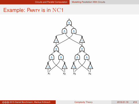
Example: Parity is in NC1

x1 x2 x3 x4

However, we also have the following major result (without proof):

Theorem 18.4 (see Arora/Barak, Chapter 14)

Parity is not in AC0, and therefore AC0 ( NC1.



http://korrekt.org/



Example: FOL model checking

FOL Model Checking

Input: First-order sentence ϕ; finite first-order structure I

Problem: Is ϕ satisfied by I?

We showed that this problem is PSpace-complete. It turns out that thiscomplexity is caused by the formula, not by the model:

FOL Model Checking for ϕ

Input: A finite first-order structure I.

Problem: Is ϕ satisfied by I?

Theorem 18.5 (see course Database Theory, Summer 2016, TU Dresden)

For any first-order sentence ϕ, FOL Model Checking for ϕ is in AC0.



http://korrekt.org/



Relationships to Other Complexity Classes (1)

Using the assumption of uniformity, we can solve circuit complexityproblems by (1) computing the circuit and (2) evaluating it.

The following are not hard to show:

Theorem 18.6 (Sipser, Theorem 10.41)

NC ⊆ P

Theorem 18.7 (Sipser, Theorem 10.39)

NC1 ⊆ L



http://korrekt.org/



Relationships to Other Complexity Classes (2)

Conversely, some known classes are also subsumed by NC:

Theorem 18.8

NL ⊆ AC1

Proof notes.General proof idea: (1) construct a “generalised” configuration graph for an NL machine (agraph that describes all possible configuration graphs using transitions that depend on theactual input that is given); (2) check reachability of the goal state in this graph (basically byrepeated matrix multiplication in the reachability matrix).We do not give a proof here. Sipser (Theorem 10.40) sketches the proof for NL ⊆ NC2;the proof for NL ⊆ AC1 is the same but also uses that the depth is only logarithmic if wecan use unbounded fan-in gates. �

We therefore obtain the following picture:

AC0 ⊂ NC1 ⊆ L ⊆ NL ⊆ AC1 ⊆ NC2 ⊆ · · · NC ⊆ P



http://korrekt.org/


Circuits and Parallel Computation P-Completeness

P-Completeness



http://korrekt.org/



The Limits of Parallel Computation

NC defines a hierarchy of efficiently parallelisable problems in P

Are all problems in P efficiently parallelisable?

Nobody knows

State of the art:

It is not known if NC , P or not

It is not even known if NC1 , PH or not

It is clear that AC0 , P (since AC0 ⊂ NC1)

It is clear that NC , PSpace (exercise: why?)

“Most experts believe that” NC , P{ if this is true, then some problems in P cannot be parallelised efficiently



http://korrekt.org/



The Limits of Parallel Computation

NC defines a hierarchy of efficiently parallelisable problems in P

Are all problems in P efficiently parallelisable?Nobody knows

State of the art:

It is not known if NC , P or not

It is not even known if NC1 , PH or not

It is clear that AC0 , P (since AC0 ⊂ NC1)

It is clear that NC , PSpace (exercise: why?)

“Most experts believe that” NC , P{ if this is true, then some problems in P cannot be parallelised efficiently



http://korrekt.org/



P-Complete Problems

Recall the definition from Lecture 15:

Definition 12.9A problem L ∈ P is complete for P if every other language in P islog-space reducible to L.

If NC , P then P-complete problems are tractable butnot efficiently parallelisable and therefore inherently serial.



http://korrekt.org/



Circuit Evaluation is P-complete

Circuit Value

Input: A Boolean Circuit C with one output, andan input word w ∈ {0, 1}n

Problem: Does C return 1 on this input?

Theorem 18.9Circuit Value is P-complete.

Proof.Membership is easy. For completeness, we reduce the word problem ofpolynomially time-bounded Turing machines. A circuit for this problem wasconstructed in the previous lecture for Theorem 17.7. This circuit family islogspace-uniform (as already remarked in Theorem 17.13), so we get alogspace-reduction. �



http://korrekt.org/



Propositional Horn Logic

A problem that is closer to artificial intelligence:

A propositional fact is a formula consisting of a single propositionalvariable X

A propositional Horn rule is a formula of the form X1 ∧ X2 → X3

A propositional Horn theory is a set of propositional Horn rules andfacts

The semantics of propositional Horn theories is defined as usual forpropositional logic.

Prop Horn Entailment

Input: A propositional Horn theory T and apropositional variable X

Problem: Does T entail X to be true?



http://korrekt.org/



Propositional Horn Logic is P-Complete

Theorem 18.10Prop Horn Entailment is P-complete.

Proof sketch.One can give a direct Turing machine encoding:

We use propositional variables to represent configurations as for Cook-Levin

We encode TM behaviour directly, e.g., for transitions 〈q, σ〉 7→ 〈q′, σ′, d〉 we can userules like Qq,t ∧Pi,t ∧Si,σ,t → Qq′ ,t+1 ∧Pi+d,t+1 ∧Si,σ′ ,t+1 (for all times t and positions i)

We do not need rules that forbid inconsistent configurations (two states at once etc.):Horn logic has a least model, and we don’t need to worry about other models whenchecking entailment

Disjunctive acceptance conditions (“accepts if there is some time point at which isreaches an accepting state”) can be encoded by many implications (one for eachcase) without “real” disjunctions

For details, see Theorem 4.2 in Dantsin, Eiter, Gottlob, Voronkov: Complexity and

expressive power of logic programming (link). ACM Computing Surveys, 2001. �


http://cmpe.emu.edu.tr/bayram/courses/531/forpresentation/p374-dantsin.pdf

http://cmpe.emu.edu.tr/bayram/courses/531/forpresentation/p374-dantsin.pdf


http://korrekt.org/



Complexity vs. Runtime

Horn logic is P-complete:

One of the hardest problems in P

Inherently non-parallelisable

However:

Prop Horn Entailment can be decided in linear time[Dowling/Gallier, 1984]

This does not imply that all problems in P have linear time algorithms



http://korrekt.org/


complexity theory - lecture 24: circuits and parallel ... · circuits and parallel computation...

Documents