complexity models for incremental computation* - ku...
TRANSCRIPT
Theoretical Computer Science 130 (1994) 203-236
Elsevier
203
Complexity models for incremental computation*
Peter Bro Miltersen** Computer Science Department, DAIMI. Aarhus University, Ny Munkegade. Bldng. 540,
DK-8000 Aarhus C, Denmark
Sairam Subramanian*** Department of Computer Science, Brown University. P.O. Box 1910, Providence, RI 02912-1910,
USA
Jeffrey Scott Vitter*** Department qfcomputer Science, Duke University, P.O. Box 90129, Durham, NC 27708-0129, USA
Roberto Tamassia+ Department of Computer Science, Brown University, P.O. Box 1910. Providence, RI 02912-1910,
USA
Abstract
Miltersen, P.B., S. Subramanian, J.S. Vitter and R. Tamassia, Complexity models for incremental
computation, Theoretical Computer Science 130 (1994) 2033236.
We present a new complexity theoretic approach to incremental computation. We define complexity
classes that capture the intuitive notion of incremental efficiency and study their relation to existing
complexity classes. We show that problems that have small sequential space complexity also have
small incremental time complexity.
Correspondence to: P.B. Miltersen, Computer Science Department, DAIMI, Aarhus University, Ny Mun- kegade, Bldng. 540, DK-8000 Aarhus C, Denmark.
*This paper reports the combined work of research efforts that have appeared in shortened form in “A
complexity theoretic approach to incremental computation”, by S. Sairam, J.S. Vitter, and R. Tamassia (STACS ‘93), and “On-line reevaluation of functions”, by P.B. Miltersen (Tech. Report, Aarhus Univ.).
** Supported in part by the ESPARIT II Basic Research Actions Program of the European Community under contract No. 3075 (project ALCOM).
***Supported in part by NSF PYI award CCR-9047466 with matching funds from IBM, by NSF
research grant CCR-9007851, by Army Research Office grant DAAL03-91-G-0035 and by the Office of
Naval Research and the Defense Advanced Research Projects Agency under contract NOOO14-91-J-4052, ARPA order 8225.
‘Supported in part by an NSF research grant CCR-9007851, by Army Research Office grant DAAL03- 91-G-0035 and by the Office of Naval Research and the Defense Advanced Research Projects Agency under
contract NOOO14-91-J-4052, ARPA order 8225.
0304-3975/94/$07.00 0 1994-Elsevier Science B.V. All rights reserved SSDZ 0304-3975(93)E0214-0
1. Introduction
What is the “best” algorithm for a given problem? There is obviously more than one
answer, depending on what we mean by “best.” If we consider worst-case time
behavior, traditionally an algorithm is considered the best possible if it meets the
information theoretic lower bound. There is another way of looking at the situation,
wherein we are not worried about the time taken to evaluate every instance from
scratch. We ask that once the algorithm has preprocessed an instance of the problem,
it should handle any changes to the instance very fast.
In Section 2 we formalize these notions in terms of the classes incr-POLYLOG-
TIME, the class of problems whose dynamic versions are solvable in poly-logarithmic
time, and incr-POLYLOGSPACE, the class whose dynamic versions can be solved
with poly-logarithmic work space. We also give a restricted notion of nondeterminis-
tic incremental computation. We show that if a problem can be solved sequentially
with a small amount of work space then there exists an efficient dynamic algorithm to
solve the same problem. We then introduce the concept of an incrementul reduction
between problems, and we present problems that are incrementally complete for other
existing complexity classes under such a reduction.
In Section 3 we show that commonly known P-complete problems (under LOG-
SPACE reductions) are incr-POLYLOGTIME-complete for the class P. We further
prove that all nonredundant P-complete problems are incr-POLYLOGTIME-com-
plete for P. This suggests that problems that are hard to parallelize are hard to
dynamize. We also show that a variant of transitive closure is incr-CONSTANT-
TIME-complete for NLOGSPACE and give similar problems which are incr-CON-
STANTTIME-complete for LOGSPACE and NC’. In Section 5 we demonstrate that
under certain restrictions, problems which have efficient dynamic solutions also have
efficient parallel solutions.
In Section 4 we consider a nonuniform model of incremental computation and show
that in this model most problems have almost linear complexity. In addition, we present
some techniques for lower bounding the complexity of explicitly defined problems.
Complexiry models,fir incremental computation 205
In Section 6 we look at incr-LOGSPACE; the class of problems that can be
“updated” using only logarithmic work space. This is an interesting class because
problems in this class are amenable to fast parallel updates (since LOG-
SPACE E NC*). We show that the circuit-value problem for comparator gates,
discussed in Mayr and Subramanian [ 1.51 is in incr-LOGSPACE while the network
stability problem is in relativized incr-LOGSPACE with respect to an NLOGSPACE
oracle. Since these problems have no known efficient parallel solutions, we get a new
class of problems which seem to be somewhat more sequential in nature than the
problems in NC but nonetheless exhibit a degree of parallelism absent in P-complete
problems. In Section 7 we present the conclusions and some open problems.
2. Preliminaries
Informally, we want a decision problem n to belong to the class incr-TIME [f(n)] if
we can “react” to the changes in a given instance of the problem in time proportional
tof(n) where n is the size of the problem statement. First we take some time to build
a data structure for an initial instance of the problem. After that point we are required
to react to any one-bit change in the current instance in time O(f(n)); i.e. we should
calculate the solution for the new instance and update the current data structure all in
time O(f(n)).
Let rc be a decision problem. An n-bit instance I of rc is any n-bit string of zeros and
ones. An instance I is said to be a positive instance if a decision procedure for
rc outputs a 1 given I as the input. A single bit change to an instance Z would involve
flipping some bit of Z from 0 to 1 or vice versa. We define the size of an incremental
change d to an instance Z (where A changes I to I’) to be the number of bits of Z that
are flipped. Another reasonable model of incremental change would be one that
allows one to insert and delete “zeros” and “ones” at various points in I. Ideally we
would like to use a definition that measures an incremental change by the minimum
amount of information needed to convert Z to I’, but that would involve issues of
Kolmogorov complexity, which would not allow concrete time or space complexity
results.
Our replacement model that we define above, where we can replace various bits of
Z by “zeros” or “ones,” is a reasonable measure of incremental change and at the same
time a sufficiently simple model for developing a theory of incremental complexity. In
the remainder of the paper we only deal with the replacement model of incremental
computation.
A dynamic algorithm for solving a problem rr will have two stages: the preprocessing
stage and the update stage. Given an initial instance Z”, in the preprocessing stage, the
algorithm constructs an internal data structure D, D associated with the instance I’.
The data structure DIo is just the portion of the internal state of the algorithm A (after
it processes Z”) that is carried over to the next stage. In the update stage, given an
incremental change A to the current instance I, the algorithm computes the answer to
206 P.B. Miltersen rt a[
the new instance I’ and makes changes to the internal data structure DI to get DIs. The
data structure D, is the portion of the internal state of the algorithm (after the instance
I has been processed) that is carried over to the next stage. We will use the term
current instance to denote the instance I that was encountered last by the algorithm,
and the term current data structure to refer to the associated internal data structure D,
constructed by A when it processes the instance I.
Strictly speaking the notation DI is not entirely appropriate since the relevant
portions of the internal state (after I has been processed) depend not only on I but also
on the algorithm A, the initial instance 1’, and the sequence of updates that were used
to arrive at I. We will use the notation Df when we want to disambiguate between two
algorithms but wherever there is no ambiguity we will continue using the notation DI
in the interest of not overloading the symbols with too many subscripts and super-
scripts.
Definition 2.1. A decision problem rt belongs to the class incr-TIME [f‘(n)] if there are
RAM programs PI and P, such that for all nEN we have
(I) Given any initial n-bit instance I0 of rr, PI efficiently precomputes some internal
data structure DIo associated with instance I’.
(2) Given the current input instance I, the incremental change d to I and the
current data structure DI in the random access memory, P, determines ~(1’) and
modifies D, into the new data structure DI, in O(ld if(n)) time.
Our notion of “efficient” in condition 1 is somewhat flexible; we could require that
the precomputation be doable in polynomial time or logarithmic space, for example.
The RAM programs are allowed to operate on 0 (log n) length words in constant
time, where n is the size of the problem instance. They are therefore allowed to read,
write, add and subtract 0 (log n) length words. The program counter is also allowed to
transfer control to an arbitrary address (e.g. to execute a jump).
We denote by incr-POLYLOGTIME the class
,Ib incr-TIME [logk n] I
We believe that such a definition captures the intuitive notion of incremental compu-
tation; e.g. the problem of maintaining an ordered set through a set of updates of
queries is in incr-TIME [log n]. Given the technical inconvenience in making the data structure an explicit part of
the definition one might argue that we do not mention the data structure explicitly but
simply state that the updating program P2 be allowed 0( 1 A if(n)) time to modify its
internal state. We have chosen to make the data structure an explicit part of the
definition because doing so allows us to control the kind of access that we allow the
updating procedure P2 to have on the current data structure. For example, in defining
the class incr-SPACE [.f(n)] we allow Pz a read-only-access to the current data
structure thus limiting the amount of work space that it can have.
Complexity models for incremental computation 207
Definition 2.2. A decision problem n belongs to the class incr-SPACE [f(n)] if there
are RAM programs Pi and Pz such that for all HEN we have
(1) Given any initial n-bit instance I0 of rc, P1 efficiently precomputes some internal
data structure D10 associated with instance IO.
(2) Given the current input instance I, the incremental change d to I and the
current data structure D1 in a read-only memory, P2 determines ~(1’) and constructs
the new data structure D1, on a write-only memory while using only 0( 1 A If(n)) work
space.
We denote by incr-LOGSPACE the class incr-SPACE [log n], and define incr-
POLYLOGSPACE in a manner similar to incr-POLYLOGTIME.
To extend these notions to nondeterminism we allow the update procedure P,
access to some nondeterministic decision oracle S. The decision oracle S can be used
by P2 to ask queries regarding the current input I and the current data structure D,.
P2 is allowed to make a polynomial number of calls to S. By restricting P2’s access to
decision oracles that are allowed to operate in NLOGSPACE we get the following
definition for rincr-LOGSPACE(NLOGSPACE).
Definition 2.3. A decision problem n belongs to the class rincr-LOGSPACE(NLOG-
SPACE) (read as n is in incr-LOGSPACE relative to the class NLOGSPACE) if there
are RAM programs P1 and P2 such that for all neN
(1) Given any initial n-bit instance I0 of 7~, P1 efficiently precomputes some
auxiliary data structure D1o associated with instance I’.
(2) Given the current input instance I, the incremental change A to Z and the
current data structure D1 in a read-only random access memory, P2 determines n(Z’),
and constructs the new data structure D, I (output to a write-only memory) while using
0( 1 A 1 log(n)) work space.
The update procedure P2 is allowed to make a polynomial number of calls to some
nondeterministic decision oracle S that uses 0 (log n) work space. P2 can take the help
of the decision oracle S in determining rc(Z’) and for making decisions about how to
construct D1 ,.
We now show that problems which can be solved sequentially using small amounts
of work space can be incrementally solved using small amounts of time per
update.
2.1. Incremental execution of space bounded computations
Standard techniques give that a nondeterministic s(n)-space bounded computations
can be simulated from scratch on a RAM in time O(n2°‘“‘““). In an incremental
setting, we show that for small (sublogarithmic) space bounds the cost of updating
208 P.B. Miltrrsen et al.
a solution is much smaller than the cost of constructing it from scratch. For instance,
as a corollary to the following theorem, NSPACE [log log n] c incr-POLYLOG-
TIME.
Theorem 2.4. Let s(n) be a space bound that can be computed in no(l) time such that
s(n) = O(log n). Then, NSPACE [s(n)] z incr-TIME [(log n)2°(S(“‘)].
Proof. Consider the computation of a nondeterministic Turing machine M on
a fixed input .Y =x x 1 2 . . . x,. We assume that the input is given on a read only
input tape with a blank symbol # at the beginning and the end. Put x0=x,+ 1 = #.
We can assume that the head on the input tape does not leave the segment
XIJX, . x,+1 during the computation. Furthermore, by changing the finite
control, we can assume that M accepts by letting the head on the input tape
leave the segment at the end of the computation, and rejects by staying inside the
segment. By a semi-con$guration of M we mean a description of the content of each
work tape and the position of each work tape head, but with content and head
position of the input tape omitted. Let S denote the set of semi-configurations of M.
Given a segment xi. . .~j of the input tape, consider the following binary relation
Ri,j between S x {l, r> and S x {L, R 1 think of 1 and r as denoting “enter from the left”
and “enter from the right”, respectively, and L and R as denoting “exit to the left” and
“exit to the right”):
l (u, l)Ri.j(o, R) iff when M is started with the input head in cell Xi while in semi-
configuration u there is a computation where the input head leaves the segment
Xi.. .~j for the first time by moving from .Xj to Xj+, while the machine enters
semi-configuration L’.
l (u,r)Ri,j(ti, L) iff when M is started with the input head in cell Xj while in
semi-configuration u there is a computation where the input head leaves the
segment xi . . . Xj for the first time by moving from xi to ximl while the machine
enters semi-configuration c.
l (u, l)Ri, j(~l, L) iff when M is started with the input head in cell Xi while in semi-
configuration u there is a computation where the input head leaves the segment
_yi . xj for the first time by moving from Xi to xi_ 1 while the machine enters
semi-configuration u.
l (u,r)Ri, j(c, R) iff when M is started with the input head in cell Xj while in semi-
configuration u there is a computation where the input head leaves the segment
Xi.. .. Yj for the first time by moving from .xj to xj+ 1 while the machine enters
semi-configuration ~3.
Suppose we know Ri,k and RCk+ 1,, j for some i 6 k <j and we want to compute Ri. j.
Let R1=Ri,k and R2=Rtk+I,,j. Consider the directed graph G =( V, E) with
nodes
V=Sxjl,r,L,R,m,,m,)

Complexity models for incremental computation 209
and edges given by the following rules:
Let R be the binary relation from S x {l,r} to S x {L, R} defined by taking the
transitive closure of G and restricting it to this domain. We refer to R as the
concatenation RI *R2 of RI and R2. It is easily seen that if i< k < j then
Ri,j=Ri,k*Rck+i),j. This suggests the following data structure: Given a tape segment
Xi ... Xj, we maintain a representation of the relation Ri,j by recursively maintaining
Ri,k and Rk+l,j where k=Lq]. The segments Xi . Xj for which the relation Ri, j is
kept form a binary tree of height O(log n). Since we keep a representation of Ro,,+ 1 we
can decide membership of L in constant time. When a letter Xi in the input is changed,
we only have to recompute each of the Rj,k in the data structure for which j< i d k, i.e.
0( log n) updates on relations on sets of size 2 o(S(n” Each update is a transitive closure .
which can be done in polynomial time, i.e. the entire operation takes time
O((logn)2°‘“‘“” ). Furthermore, by the assumption on s(n), the data structure can be
initialized in time no”‘. 0
2.2. Incremental reductions
To compare the “hardness” of solving two problems in this incremental sense,
we need the notion of incremental reduction. It is clear that the program doing
the reduction from problem rcl to problem rc2 has to be incremental in the same
sense as the RAM program P, in Definition 2.1. In the same way as before we
allow some computation to construct a data structure to an initial instance
of rci and to find the corresponding instance of z*. We then require that any
change to the current instance of n, be reflected as a change to the correspond-
ing instance of x,, within a stated time limit. There are however two differences
since we are now dealing with functions (in the previous case the solution was
always a “yes” or a “no”) which map instances of nl to instances of 7c2. We
need to quantify the relative sizes of the corresponding instances as well as the
amount of change the mapping undergoes when the input changes by a specified
amount.
We take care of these by introducing two more parameters to quantify a
reduction.
210 P.B. Miltersen et (11.
Definition 2.5. A decision problem 7c1 is incrementally reducible to another deci-
sion problem 7c2 with time and size bounds [f(n), g(n), p(n)], denoted
x1 6 incr[f(n~,y(n~,p(n)~ ~2, if (1) There is a transformation T: 7~~ -+ z2 that maps instances of 7c1 to instances of 7~~
such that for any n-bit instance Z of x1 the size of the corresponding instance T(Z) of 7r2
is bounded above by p(n). Furthermore, Z is a positive instance of 7c1 if and only if T(Z)
is a positive instance of x2.
(2) There are RAM programs P and Q such that for all n30 we have
(a) Given any n-bit initial instance I0 of n,, P efficiently computes T(Z”) and some
auxiliary data structure S1o associated with I’.
(b) Given the current instance I, the incremental change A 1 to Z (where A 1 changes
I to I’ of 7~~) and the current data structure S, in the random access memory,
Q constructs the incremental change A2 to T(I) (where A2 changes T(Z) to T(Z’)), such
that 1 A2 1 < g(n) 1 AI 1, and modifies S, into the new data structure S,, in O(/AI If(n))
time.
Note that y(n) is always O(f(n)).
We use the symbol S, to denote the data structure maintained by the transforma-
tion T so as to differentiate it from DI which is the data structure associated with an
algorithm that solves a given problem 7~.
Theorem 2.6. Zf x1 is incrementally reducible to 7c2 in time and size bounds
[f(n),g(n), p(n)], and if 7r2 is in incr-TIME[k(n)], then 7t1 is in incr-
TIME U(n)+ Wn))s(n)l.
Proof. We now give a dynamic algorithm B to solve 7~~ that is a composition of the
transformation T (from 7cn, to 7c2) and the dynamic algorithm A that solves 7c2 in
incremental time ,f(n). The basic idea is as follows: We run the transformation
algorithm Tin the background and whenever the current instance Z of x1 changes, we
use T to compute the incremental change to the corresponding instance T(Z) of 7r2 and
feed that change to algorithm A. By the definition of the transformation the answer
given by A is also the answer for the modified instance I’ of 71,.
More specifically, in the preprocessing stage, given the initial instance I’, we start
the background transformation T that maps I0 of x1 to the corresponding instance
T(Z’) of n2. We now also start the dynamic algorithm A, for solving n2, with T(Z’) as
the initial instance. The internal data structure of B is therefore a combination of the
internal data structures S1o of the transformation algorithm T and T,o of the algo-
rithm A. In other words D~o=S~OUD$(,O,.
By the definition of the transformation T, x2( T(Z’)) is the same as x1(1’). Therefore
the initial computation on T(Z’) computes 7c1 (Z’).
Given an incremental change AI to the instance I, we first use the dynamic
transformation algorithm T to compute the incremental change A2 to T(Z) in time
0( I Al If(n)) time. At this time the data structure S1 is modified to reflect the change in
the input. Then, we give A2 as input to the dynamic algorithm A, which computes
Complexity models ,for incremental computation 211
nz(7(Z’)) and modifies the data structure DATcr, to get DA,,,,,. By definition
rc2( T(Z’))=rc,(I’) therefore the answer returned by A is correct.
By construction 1 A2 1 d 1 A 1 Is(n). Also, since the size of T(I) is no more than p(n) and
rc2 is in incr-TIME [h(n)], algorithm A takes 0( I A2 I h(p(n))) = 0 (I A 1 I g(n)h(p(n)))
time to modify DA,(,) and to compute rcz (T(Z’)). Therefore, the time taken to compute
rci(l’) and to modify 0: is the time for computing A2 summed with the time required
by algorithm A to compute rc2 (T(I’)). Thus the total time for the updating process is
O(lAl If(n)+lA,Ih(p(n))g(n)). Hence, rrl is in incr-TIME[f(n)+k(p(n))g(n)]. 0
3. Incrementally complete problems
We now turn to the notion of incremental completeness. The idea is to find
a problem which is hard to solve incrementally as any other problem in a given class.
In this section we use incremental reductions to get natural problems incrementally
complete for P, NLOGSPACE, LOGSPACE, and NC’.
Definition 3.1. A problem 7c is said to be incr [,f(n), g(n), p(n)]-complete for a class C if
(1) rr is in the class C.
(2) For all 7c1 in C, rcl is incrementally reducible to rc in time and size bounds
Cf(47s(n),P(n)l.
We call a problem 7c incr-POLYLOGTIME-complete for a class C if rr is
incr [f(n),g(n),p(n)]-complete for C, where p(n) is bounded above by some poly-
nomial in n, andf(n) and g(n) are 0 ( logk n) for some k. We define incr-CONSTANT-
TIME-completeness in an analogous fashion.
The obvious question to explore is how the complexity classes incr-POLYLOG-
TIME, incr-POLYLOGSPACE, and incr-LOGSPACE are related to the well known
sequential complexity classes? Our first intriguing result is that the commonly known
P-complete problems listed in [18, lo] are incr-POLYLOGTIME-complete for the
class P. These problems include the circuit-value problem (CV), the solvable path
system problem (SPS), propositional horn satisfiability, and a host of other well
known P-complete problems. These problems are therefore as hard to solve incremen-
tally as any other problem in P.
Theorem 3.2. AI/ P-complete problems in [18, lo] are incr-POLYLOGTIME-complete
for the class P.
Proof. We present the proof for the case of circuit-value problem. In this problem we
are given a directed acyclic graph as the input. A node in this graph is either labeled an
input node or an output node, or it corresponds to a gate in the circuit. A gate could be
AND, OR, or NOT gate. The edges in the graph correspond to wires of the circuit. All
the input nodes have in-degree zero and out-degree one and all the output nodes have

212 P.B. Miltersen et al.
in-degree one and out-degree zero. The AND and OR gates have in-degree at least
two and out-degree at least one while the NOT gate has both in-degree and out-
degree equal to one. Given an assignment of zeros and ones to the input nodes and
a specific output node X, our aim is to find the value of the output node. In other
words our aim is to find the value of the output wire attached to X given a particular
assignment to the input wires of the circuit.
To prove that the circuit-value problem is incr-POLYLOGTIME-complete for
P we proceed as follows: Given any problem rr in P and an initial instance 1’ with
/ 1 ‘I< n, we use the standard LOGSPACE reduction 1141 to create a circuit of size t(n)
by t(n) (where t(n) is a time bound for some polynomial-time turing machine M to
solve instances of 71 of size at most n) that simulates the turing machine M used to
solve the problem TC.
The inputs to this circuit are the bits of the initial instance 1’. This gives us the
initial transformation of 1’. A one bit change to I0 results in a one bit change to the
corresponding instance of the CV (the input variable in the circuit corresponding to
the changed bit is changed to reflect the new input). All this can be done in constant
time, and thus the circuit-value problem is incr-POLYLOGTIME-complete
for P.
We can provide similar proofs for the other problems listed in [18, lo]. The
reductions needed to show this are sometimes different from those given in the
literature. The modifications are minor and are needed to ensure the following
property: For the reduction to be incremental we require that when a general problem
rc in P is changed by one bit, input to the incrementally complete problem under
consideration changes only by a polylog number of bits. The use of preprocessing
plays a significant role, since the size of the instance of the incrementally complete
problem may be a polynomial factor larger than the problem rc in P. 0
Corollary 3.3. [f the P-complete prohlerns in [ 18, lo], like circuit-value problem, are in
incr-POLYLOGTIME then all qf P is in incr-POLYLOGTIME.
Corollary 3.4. Jf there are NC algorithms to update dynamically the P-complete
problems in [ 18, lo], then tile automatically yet NC algorithms to update dynamically all
of P.
These corollaries suggest that it is highly unlikely that we can use polylogarithmic
time sequential or parallel algorithms to incrementally update these problems.
Delcher and Kasif [S] propose other notions of completeness. They define the
incremental version of a functionf‘as follows: Letf be a function that maps input X of
length 1x1 to output f(X). Then Inc .f’ is the function that given inputs of form
(X,,f(X), X’), computes ,f (X’), where X and X’ differ in at most log /X 1 bits. A func-
tion f is Inc P-complete iff for every function g in P, Inc g is LOGSPACE-reducible to
IncJ With this definition they argue that the “all-outputs monotone circuit value
problem” is Inc-P-complete. The drawback in this approach is that it disallows the use
Compiesity mod&for incremental computation 213
of dynamic data structures. In other words their incremental reductions are not strong
enough to conclude that it is unlikely that one will get good algorithms (meaning NC
algorithms) for the incremental versions of Inc-P-complete problems irrespective of
the size of the auxiliary storage. They try to overcome this drawback by proving that
the incremental versions of many P-complete problems are also P-complete. Here
they completely ignore the issue of preprocessing. Although their results are interest-
ing, they are somewhat weak in that the issues of data structures and preprocessing
are overlooked. They conjecture that the incremental versions of all P-complete
problems are P-complete.
Interesting notions of completeness are sketched by Reif [21]. He shows that some
problems are unlikely to have efficient incremental solutions, but he does not develop
a comprehensive theory or consider the necessary details of preprocessing. Some
interesting techniques are explored in [Z, 6,201 to derive lower bounds for incremental
algorithms. Their main idea is to construct an algorithm for the batch version of the
problem with input I by computing a dynamic data structure for some easily
computed instance I’, whose Hamming distance from I is small, and then applying the
incremental algorithm repeatedly while I’ is successively modified to I. This gives
lower bounds for the incremental problem in terms of that for the batch problem. The
drawbacks of this approach are that it limits the amount of preprocessing available
and is problem specific.
Theorem 3.2 would seem to suggest that all P-complete problems are incr-POLY-
LOGTIME-complete for P. Unfortunately that is not the case, since one can take any
incr-POLYLOGTIME-complete problem ‘II and create another problem rc’ by du-
plicating the input, so that 7~’ is no longer incr-POLYLOGTIME-complete even
though it is still P-complete. In fact we prove that some P-complete problems can be
solved effectively incrementally.
Theorem 3.5. There are P-complete problems that are in incr-POLYLOGTIME.
Proof. Let L be some P-complete language over the alphabet C = {0, 1} such that it
takes linear sequential time to determine whether a given word M? is in L or not (the
restriction to languages that can be recognized in linear time is only made for the sake
of convenience, the same can be done with any P-complete language). Let us consider
the language L’ = {w I wi 1 WEL). Obviously L’ is also P-complete. We claim that
membership queries for L’ can be performed dynamically. We will abuse notation
slightly by using the symbol L’ both for the language and the associated membership
problem. Consider an initial n2-bit instance 1’ of the problem L’ (instances which are
not of the form n2 for some nEN can be handled without too much trouble). We spend
polynomial time to see if it is of the form WI”’ for some WEL. This, we can do by
running a subroutine SL to check membership in L and some associated linear time
work to see if I0 is of the form w IwI. At any point in time let the current instance I be
a concatenation of n bit strings a,, a2, . . . , a,. The idea behind our dynamic algorithm
is as follows.

214 P.B. Miltmrn et a/
As long as less than n/2 of the ai’s are equal (i.e., less than n/2 of the strings
are the copy of the same string w) we answer “no” for every instance. If at some
point more than n/2 of the ai’s are all equal to the same w, we start a background
process which executes the subroutine SL on the string w. As long as more than half
the ai’s are equal to w we spend a constant amount of time on the background
computation for every update to the current instance. Therefore, by the time I be-
comes equal to wlw’ we would have run S, for a linear number of steps and thus will
know whether w is in L or not. We can therefore answer the membership query of I in
L’ at that point.
It seems hard to dynamically figure out whether more than half the Ui’S are all equal
to the same w. Therefore, we perform the following easier computation.
(1) The data structure. We divide each a, into k= n/log n words u&z!,
each of which is composed of logn consecutive bits from Ui. We now construct k
sets Si, Sz, . . . , Sk such that the set Sj contains the ,jth word from each ui. In
other words Sj=(U{,a$, ,a;>. With each set Sj we maintain two flags f;: and
gj. The flag ,J is set to 1 if more than half the words in that set become equal
to the same word wj, otherwise it is set to 0. The flag gj is set to 1 if all the
words in Sj are the same, otherwise it is set to 0. The word wi associated with
Sj is called the majority word of Sj. If the flagfj of Sj is 0 then wj is set to a string of log n
0’s. We also maintain a string HI that is the concatenation of wl, w*, . . . , wk in that
order.
(2) The algorithm
l As long as at least one of the flags gi , gz, , gk is equal to 0 we answer “no” for
every instance.
l If at some point all of the jllagsj; ,f2,. . ,,ji are equal to 1, we start a background
process which executes the subroutine SL on the string w maintained by the data
structure; and from then on we simulate a constant number of steps of SL for every
update operation (the constant depends on the sequential time complexity
of L).
l It at some point one of the f flags becomes equal to 0 we abort the background
process that runs the subroutine S,,.
l If all of the g flags gl-gk are equal to 1 we get the answer to the background
computation on w from SL and return that as the answer.
By definition when all the y flags gi-gk are equal to 1 the input is of the form Wl”“.
for some W. Therefore, to prove our algorithm correct we need to prove that by the
time all the g flags become 1 the background process already has the answer to
whether W is in L or not.
To prove the correctness of our algorithm let us consider the sequence of instances
starting at Ia, going through I ‘, I *, , all the way up to the current instance I = I’ for
some I, where every instance I” is derived from the previous instance I”- ’ by updating
the bit that was changed at time x- 1. Let Zh be the instance closest to I such that it is
a concatenation of the strings a,, a *, . a, and n/2 + 1 of the u;s are equal to W. Since
at instance !I only n/2 + 1 of the Ui’s are equal to \i;, I-h >, n/2 - 1. Suppose we start the
Complexity models for incremental computation 215
background process SL on the string W at time h and execute a constant number
of its operations for every subsequent update. Since 1 -h 2 n/2- 1 and S,
requires linear time to recognize W, at instance 1 we would know whether W is in L or
not.
We now show that the algorithm outlined above will start the background process
at time h. Consider a division of W into n/log n words W’, W2, . . , Wk each of which
consists of log n consecutive bits from W. Since at time h more than half of the strings
are equal to W, for each set Sj the flagfj is set and the majority word wj of the set is
equal to G? Therefore, the string formed by concatenating all the majority words
is equal to W. Hence, our algorithm will start the background computation SL on
W at the right time thus ensuring the availability of the answer when all the g flags
become 1.
We now show in detail how the sets S1-Sk can be maintained dynamically as the
input I undergoes changes. Each set Sj is maintained at the leaves of a balanced binary
search tree Tj. The words a{, ai,, . . . , aj, are stored at its leaves in sorted order (by
treating each a{ as longn bit integer). Note that since the words are sorted all the
words that are equal to each other are stored in contiguous leaves.
Each internal node i in Tj maintains three numbers maxi, right,, and lefii and three
associated words max_wordi, left_wordi and right_wordi. The quantity maXi indicates
the maximum number of words in the subtree rooted at i that are equal to the same
word max_wordi which is the word stored at the “left-most” leaf in the subtree rooted
at i, while right, is equal to the number of words that are equal to the word right-word, which is the word stored at the “right-most” leaf in the subtree rooted at i. We also
store a value totali that is equal to the total number of leaves in the subtree rooted
at i. Let z be an internal node in q, and x and y be, respectively, the left and right child
of z. We can then use the following program to derive the values of total,, left=, right,, max,, left_word,, and max_word, from corresponding values at x and y:
procedure update
begin
[The default case]
total,+- total, + total,
left-word,+left-word, leftz t leftX right-word,+-right-word,
right,+-right, if (max,>max,) then
max, +- max, max_word,+max_word,
else max,+max, max_word,+max_word,
216 P.B. Milrersen et al.
[when the boundary words of x and y are the same]
if (right-word, = lefttword,) then
if (leftX = total,) then
I&,-l&, + I<&
if (right, = totul,) then
right=+right, + right, if (mu.xz <(right, + kfty)) then
mux=+-right, + kftft,
max_word,+right_word, end
end [procedure update]
Given the values at the nodes x and y these operations can be performed in constant
time to derive the values at node z. Whenever the current instance I changes by
a single bit, exactly one of the words a’, (for some x andj) changes. Therefore only one
of the sets Sj needs to be updated. The elements of Sj are stored in sorted order at the
leaves of a balanced binary search tree. Therefore, a change in one of the acs implies
we have to delete it from its current location in tree and reinsert it in another location
so as to preserve the sorted order. A delete or an add operation causes changes along
a leaf-to-root path (starting at the leaf-node that was deleted or added). However,
since the tree is balanced there are only O(logn) nodes along any leaf-to-root path.
This implies that all the values along this path can be appropriately changed in
O(logn) time to reflect the change at the leaf node. Thus the data structure can be
modified in O(log n) time to reflect a single-bit change in the current instance 1.
The above construction works by taking an incr-POLYLOGTIME-complete prob-
lem and introducing redundancy by copying, and in fact all the ways to generate
incrementally tractable problems from P-complete problems seem to involve redund-
ancy in some form or the other. We restrict ourselves therefore to P-complete
problems that are in some sense nonredundant. To do that we first look at a much
stricter definition of P-completeness; one in terms of projections, introduced by
Skyum and Valiant [22].
Definition 3.6. A decision problem rcr is projection reducible to unother decision
problem 7~2 (n I< proj ?I 2 ) if there is a function p(n) bounded above by a polynomial in n,
and a polynomial time computable family of mappings 0 = (cI,( i,n3 1 where
such that for any n-bit instance I of rcl we can derive a p(n)-bit instance I’ of 7c2 using
the mapping cm. The mapping has the property that I is a positive instance of 7c1 if and
only if I’ is a positive instance of rr2. To derive I’ we give xi the same value as the ith bit
of I and use O,(yi) as the bit of I’. We say that 0 is bounded above by p and rcl is
o-reducible to rr2.

Complexity models for incremental computation 217
Definition 3.7. A problem 71 is said to be <proj- complete for a class C if 7~ is in C and
there is a function p(n) bounded above by a polynomial in n such that every problem
x1 EC is projection reducible to 71 by a projection c = {o,, }n2 1 bounded above
by P.
Problems like the circuit-value problem are < ,,,j-complete for P. Even under this
restricted setting it is possible to create problems which are < p,,j-complete for P but
are in incr-POLYLOGTIME. To remedy that we introduce the following notion of
nonredundancy.
Definition 3.8. Let 7c1 be a decision problem and n be another problem such that
7(1 Gproj T-C. We say that n is nonredundant with respect to 7c1 if there exists a polynomial
time computable family o = IO,,},, 31 of mappings and a number kEN such that z1 is
a-reducible to 7~ (where cn is a mapping from the set (y,, .._, yp(,,)) to
{- ,, x1,x1, ..., X,,X 0, l}), and for all symbols Xi, 10,’ {Xi, xi} j = O(logkn).
Intuitively the reduction from x1 to n is nonredundant if in the projection mapping
a single bit xi of xl does not affect more than O(polylog(n)) bits of 7~.
We now define the notion of nonredundancy with respect to a class C.
Definition 3.9. Let 71 be a problem which is <p,,j-complete for C. We say that n is
nonredundant with respect to C if it is nonredundant with respect to every problem in
C. We then call x a nonredundant projection complete problem (or a NRP-complete
problem) for the class C.
Lemma 3.10. Let C be a class of decision problems and let nI be a NRP-complete
problem for C. If n is another decision problem in C such that x1 <proj~ and 71 is
nonredundant with respect to x1 then x is NRP-complete for C.
Proof. The proof follows from the definitions in a straightforward manner. 0
Th P-complete problems listed in [ 18, IO] are all NRP-complete for P. The
following theorem shows that this large class of P-complete problems are difficult to
make efficient incrementally.
Theorem 3.11. Let C be a class @“decision problems and K be an NRP-complete problem
for C, then 7c is incr-POLYLOGTIME-complete for C.
Proof. The proof follows from noting the fact that given any problem x~EC, there is
projection mapping from TZ to z1 (that can be computed in the preprocessing stage)

218 P.B. Miltersen et al.
such that a one bit change in an input instance of xi causes at most polylog number of
bits to change in the corresponding instance of 7~. 0
We now look at the classes NLOGSPACE, LOGSPACE, and NC’.
Theorem 3.12. The following variant of transitive closure is incr-CONSTANTTIME-
complete for NLOGSPACE:
Input: A directed graph G = ( V, E) such that each eeE is colored with 0 or 1; a pair of
vertices v1 and v2; a partitioning qf V into sets VI, V2,. . . , Vk; and a color vector C of
length k.
Output: Is there a path p from v1 to v2 such that all edges in p emanating from vertices
in Vi have color C[i]?
Proof. The reduction from any problem in NLOGSPACE to this variant is straight-
forward. The trick that makes the reduction go in constant time and constant storage
is the use of the sets VI, Vz, 0, . , Vk and the color vector. We group all intermediate
states that read the input bit i into the class Vi; C[i] is assigned the same value as
input bit i. Now a change in some input bit i changes C[i]. 0
A restriction of the above problem is incr-CONSTANTTIME-complete for LOG-
SPACE while a similar variant of bounded width polynomial size branching programs
[l] gives us an incr-CONSTANTTIME-complete problem for nonuniform NC’.
Surprisingly, however, there are problems which are NC’-complete for LOG-
SPACE, but are nevertheless in incr-POLYLOGTIME. We consider the problem of
undirected forest accessibility (UFA). The UFA problem is defined as follows: Given
a forest of undirected trees (there should be at least two trees) and given two nodes
u and v, determine if they are in the same tree. This was shown to be NC’-complete for
LOGSPACE by Cook and McKenzie [4]. Thus from the point of view of parallel
computation UFA is as hard as any problem in LOGSPACE. However, as the
following theorem shows, UFA is in incr-TIME [log n] while we do not know whether
all problems in LOGSPACE can be efficiently dynamized. Thus in the dynamic
setting UFA is not the hardest problem in LOGSPACE.
Theorem 3.13. The undirected forest accessibility problem is in incr-TIME[logn],
under additions, deletions, linking and cutting of trees.
Proof. The dynamic maintenance is done by using balanced trees such as red-black
trees to maintain ordered sets with insert, delete, split and join [ 1 l] (see also [23]).
l Preprocessing: An Euler tour of each tree in the forest is maintained in a red-black
tree. Each edge of the tree occurs twice in its Euler tour.
l Query(n,, n2): Let e be an edge in the adjacency list of n, andf’an edge in the list of
n2. We follow pointers in the red-black tree to determine if they both have the same
root.
Complexity models for incremental computation 219
l Linking and cutting are implemented using the split and join operations of red-
black trees, with O(logn) time per operation. 0
4. Nonuniform complexity
In traditional, nonincremental complexity, it has proven useful to consider comput-
ing in nonuniform models, e.g. to consider the circuit complexity of decision problems.
In this section, we consider the nonuniform complexity of incremental problems.
Given a decision problem 7c, we may consider it as a subset of 10, 1 j* and consider its
restriction ?I, to (0, l}“, i.e. we consider 71 as a family of Boolean functions. The
nonuniform model in which we consider implementing this restricted problem is the
cell probe or decision assignment tree model, previously considered by Fredman [7, S]
and Fredman and Saks [9]. In this model, the complexity of a computation is the
number of cells accessed in the random access memory containing the data structure
during the computation, while the computation itself is for free (and information
about which operation to perform is also given for free). The number of bits B in a cell
is a parameter of the model. Formally, the model is as follows: For each of the 2n
possible incremental changes (corresponding to changing each bit to either 0 or l), we
assign a decision assignment tree, i.e. a rooted tree containing read nodes and write
nodes. When performing an operation we proceed from the root of its tree to one of
the leaves. The read nodes are labeled with a location of the random access memory.
Each has 2’ sons, one for each possible content of the memory location. The write
nodes which are unary are labeled with a memory location and a value between 0 and
2’- 1. When such a node is encountered, the value is written in the memory location.
In the leaf finally encountered, the answer to the decision problem is found. The
complexity of an implementation is the depth of its deepest tree, initialization of the
data structure is for free.
Definition 4.1. If a problem z,, can be solved with cell size B and a system of trees of
depth at most d, we say that z,ECPROBE[B,d].
The model is very general, focusing on the storage and access aspect of data
structuring. We consider two natural choices of B, namely, B= 1 and B=logn.
We note that if a decision problem z is in incr-TIME[f(n)], then
x,ECPROBE [log n, 0 (f(n))]. Thus, lower bounds in the B = log n model is also lower
bounds for the complexity of solving the problem on a random access machine.
The following theorem gives tight bounds on the complexity of almost all functions.
Theorem 4.2. For any B> 1, the following holds. For any function f: (0, l)“+(O, I},
fECPROBE[B,rn/BJ 1.
Furthermore, for almost all jimctions f on this domain,
f$CPROBE[B,(n-2logn-4)/J?].
Proof. The upper bound follows from the data structure consisting of the string
xg{O, 1)” to be maintained itself. For the lower bound we only have to consider the
case B= 1. We can determine f from the system of 2n decision assignment trees
implementing the incremental version of f‘and the state of the data structure when the
value to maintain is initialized to x=0”. However, note that we may without loss of
generality assume that the initial state of the data structure consists entirely of cells
containing O’s, since we can convert an algorithm with a different initial state into such
an algorithm by “hardwiring” information about the initial state into the algorithm.
Thus, we only have to give an upper bound on the number of systems of trees of depth
d. The total number of nodes and leaves in the trees in such a system is at most
2n(2*+ l - 1)<4n2*. Thus, there are at most 4n2* cells in the data structure, we may
assume without loss of generality that these are numbered 1, ,4n2*. Each node/leaf
is either a “answer 0” leaf, an “answer 1” leaf, one of 4n2* possible read nodes or one of
8n2* possible write nodes. There are thus at most ( ln2d)4n2d systems. Therefore, there
are at most 22” ’ different systems of depth d = Ln - 2 log n - 41. There are, however,
22” Boolean functions on n inputs. c
Thus, almost all decision problems have nonuniform complexity @(n/B) and are
thus not in “nonuniform incr-POLYLOGTIME”. However, in order to make pro-
gress on the P vs. incr-POLYLOGTIME question, we have to give lower bounds for
easily computed functions.
We will present two methods giving such bounds: The first gives bounds of the type
,f$ CPROBE [ 1, o( log n)] for some special, but easily computed, functions. The idea of
the proof is very similar to Neciporuk’s method for proving lower bounds on formula
size (see Boppana and Sipser [3]): If a function has many subfunctions on a small set
of variables, it must have high complexity.
Letfbe a Boolean function on the set of variables X = (x1, .x2, . ,x, ). A subfunc-
tion of .fon Y c X is a function obtained from f by setting the variables of X - Y to
constants.
Theorem 4.3. Let f: {0, 11” -+ (0, 1 i be a function that supports s difSerent subfunctions
on a set of cariables Y of size m. Then
f$CPROBE [ 1, log log s-log log log s - log nz -41.
Proof. Let a system of decision assignment trees of depth d for the incremental version
off be given. We can get an algorithm for the incremental problem for each of the
subfunctions on Y by performing a sequence of operations from the initial state
changing the value of the variables in X - Y to the appropriate values and letting the
resulting state be the initial state of the data structure. As in the proof of Theorem 4.2,
Complexity models ,for incremental computation 221
there are at most ( 13m2d)4m2d different functions on m variables in CPROBE [ 1, d], so
we must have (1 3m2d)4m2d > s. This implies
d>loglogs-logloglogs-logm-4. 0
Let the storage access function ACCESS,+rr,s”l: (0, l}n+r’osn’+ (0, l} be the func-
tion which takes as input a bit vector x=x0x1 . . x,_ 1 E {O, l}” and a binary vector
YE{@ 11 r”snl denoting an integer i and outputs xi. Let the element distinctness
function DISTINCT,r2iopnl: {O, 1) nr2’osnl-+ (0, l} be the function which takes as
input n Boolean strings of length r21og nj and outputs 1 if and only if all strings
are distinct. Clearly, DISTINCT,r21,,.1 and ACCESSrl,s.l+, are both in
CPROBE [ l,O(log n)]. Theorem 4.3 provides matching lower bounds for these
functions.
Corollary 4.4. Neither ACCESS,+rlOg,l nor DISTINCTnr210gnl are in
CPROBE[ 1, o(log n)].
It is however, easy to see that Theorem 4.3 is unable to provide larger bound on
Boolean functions on n variables than log n - O(log log n).
Lower bounds in the B=logn model can be derived from a lower bound by
Fredman and Saks for the complexity of maintaining an array during changes and
prefix queries. Fredman and Saks [9] show that any cell probe algorithm for the
problem of maintaining a vector (x0, . . . , x, _ 1 )E (0, 1)” during change(i) opera-
tions which flip the value of xi and prefix(j) queries returning x0 @x1 @ ... @Xi
uses R(log n/loglog n) probes per operation (0 denotes exclusive or). From this
result, we get lower bounds on decision problems like the undirected forest accessibil-
ity problem. Consider the UFA problem in which we have to determine whether the
nodes 1 and n are in the same tree or not:
Theorem 4.5. UFA +! CPROBE [log n, o(log n/log log n)]
Proof. Assume that the incremental version of UFA can be solved in
0 (log n/log log n) probes. We show that the same holds for the prefix problem. We
maintain the vector (x0, x1, . . , x,_ 1) by maintaining the graph G=( V, E) with
V={1,...2n+3} and
E= U {(2i+l, 2i+3),(2i+2,2i+4)} u x,=0
xv, ((2i+ 1,2i+4), (2i+2,2i+3)}.
A change of an xi corresponds to a constant number of insertions and deletion of
edges. In order to compute x0 @xi 0 ... @ Xj, we insert the edge (2j + 3,2n + 3). If
vertex 1 and vertex 2n + 3 are in the same tree, the answer is 0, otherwise it is 1. After
getting the answer we remove the edge (2j+3,2n+3). 0

222 P.B. Miltersen et al.
Corollary 4.6. UFA 4 incr-TIME [o (log n/log log n)]
However, for no polynomial-time computable function do we know any cell probe
lower bounds better than Q(log n) (for B = 1) or Q(log n/log log n) (for I3 = log n). Once
again, we see a similarity between incremental and parallel complexity: A nonuniform
measure of parallel time is depth, and for no problem in P do we know a better lower
bound on its depth than Q(logn), although we know that most problems require
linear depth, which is also an upper bound.
5. Incremental computation in restricted realms
The class of Z-strutijed trees was introduced by Overmars [ 191 in an effort to form
a general theory of balancing in search trees. It subsumes a large portion of the search
structures used to design dynamic algorithms. In this section we show that under
reasonable assumptions problems which have incremental solutions based on these
structures also have parallel solutions.
The class of Z-stratified trees generalizes (among others) the following classes of
balanced search trees: AVL-trees, generalized AVL-trees, one-sided height-balanced
trees, power trees, 2-3 trees, B-trees, symmetric binary B-trees, height-balanced 2-3
trees, k-neighbor trees and BB[r] trees. Thus Z-stratified trees generalize a large class
of structures that are used in designing dynamic algorithms.
For the sake of completeness we now give some definitions from [19] that charac-
terize the class of Z-stratified trees. For a more complete treatment the reader is
referred to [19].
Definition 5.1. Let X be a class of balanced binary trees and for each k 30 let Xk
denote the subclass of trees in X that have height k (the height of a tree is the longest
path from the root to a leaf). X is called a-proper (for a 3 0) if and only if for each t 3 N
there is a tree in X with t leaves.
Definition 5.2. Let Z be a set of trees all of the same height fi (Z need not be a subset of
X,). Also, let L2 be the smallest and the largest number of leaves (respectively) that any
tree in Z can have. Z is a P-variety iff the following conditions hold:
(1) 1 <I=<hz
(2) For each t such that lz< t<h, there is a tree in Z with exactly t leaves.
Let r,, T2, . , 7; be trees and let T be a tree with t leaves x1, .x2, . . . ,x, from left to
right. The composition T[ Tl, T,, , T,] denotes the tree obtained by grafting Ti onto
xi for every i. In other words for each i such that 1 <i < t we replace the ith leaf xi of
T by the root of the ith tree K.
Complexity models for incremental computation 223
Definition 5.3. Let X be an x-proper class and let Z be a b-variety. We say that Z is
a regular P-variety for X iff Vt 2 a, for any tree TEX, and TI , T,, . . , T, in Z the
composition T[T,, T,, . . . . T,] is in X.
Let X be a a-proper class of trees and let Z be a regular P-variety of X. Essentially
the class of Z-stratified trees in X are the trees in X that can be formed by taking
small trees from X and building larger trees from them by layering trees from Z
using the composition operator defined above. We now make these notions more
precise.
Definition 5.4. Let X and Z be tree classes as defined above and let
k=max {aIz, rlz- l/&--lZJ}. Let y be the smallest integer such that for each t with
CL d t <k there exists a tree TEX of height at most y that has exactly t leaves (such
a y always exists). The class of Z-stratified trees (in X) is the smallest subclass of trees
satisfying the following properties:
l Each TEX of height d y with CY d t < k leaves is Z-stratified.
l If a tree T with t is Z-stratified, then so is the composition T[ TI , T,, . . . ,7;] for any
set of trees T,, T,, . . . , T,EZ.
Overmars [19] showed that the class of Z-stratified trees generalizes many other
search trees. He also showed that these trees can be used to efficiently store and search
elements in a dynamic environment, using only 0 (log n) basic operations to perform
inserts, deletes and queries. In the following theorem we show that dynamic algo-
rithms which use Z-stratified trees can be transformed efficiently into parallel algo-
rithms for the batch version of the same problem.
Theorem 5.5. Let n: be a problem in incr-TIME[logk n], for some k 2 1. Then rt is in NCki2, tf the following constraints hold:
(1) The data structure used by the dynamic algorithm is an augmented Z-strat$ed
search tree. Each internal node may contain information relevant not only to enable search but may contain the result of some function f applied to its children. The only
restriction is that f be computable in time O(logkn).
(2) There is a special instance IO such that the tree corresponding to IO can be built in
LOGSPACE.
(3) Any l-bit change to the current input I, where 1 < 1 Gn, involves modifying the tree
by inserting or removing some number of elements. The elements to be inserted or deleted arefunctions of the current input, the current data structure and the change, and they can be computed in LOGSPACE.
(4) After all the insertions and deletions some sort of search is conducted in the tree in
time O(logkn) to get the answer to the updated instance.
Proof. Given instance I we proceed as follows: First we create the tree corresponding
to I0 in LOGSPACE and calculate all the deletions and additions needed to get the

224 P.B. Milterwn et al
tree for I, also in LOGSPACE. Now we determine the order in which they are to be
present in the final tree in NC?+‘. This can be done because the function is used in
determining the order between two elements is computable in O(logkn). Therefore,
the set of elements in the tree for I can be sorted in EREWk”, and hence in NCk+’
[ 131. We then construct the tree in time NC k+2 in a bottom-to-top sweep. This can be
done because Z-stratified trees have logarithmic depth and the value of the function
,fat a node depends only on the contents of the nodes of its children. All we have to do
now is to let one processor walk down the tree and get the answer to I in time
O(logkn). 0
This deceptively simple theorem demonstrates why most known problems with
efficient dynamic solutions have optimal parallel solutions. For example, we can use
this theorem to parallelize dynamic algorithms using degree-balanced trees, height-
balanced trees, path-balanced trees, etc. We can derive similar results for other classes
of trees as well.
One important technique in getting dynamic solutions for problems is the divide
and conquer approach. To exploit this technique Mehlhorn and Overmars [16]
consider an important class of problems called order-decomposable problems.
Definition 5.6. A set problem is loosely defined as follows: Given a set V a set problem
n asks some question about V. For example, the maximum problem asks for the largest
element in a given set of numbers.
Note that in this definition rr is not necessarily a decision problem. For many set
problems it is possible to derive the answer over the total set V by combining the
answers over two, in some ways separated, “halves” of the set. Set problems of this
kind are called order decomposable. More formally, given a smooth nondecreasing
integer function C(n) we have the following definition for a C(n)-order-decomposable
set problem.
Definition 5.7. A set problem 7r is called C(n)-order-decomposable if and only if there
exists an ordering ORD (that can be used to order any input set V) and a binary
function q such that the following holds: Given a set of n> 1 points
V=(p,,p, ,..., Pn), ordered according to ORD, for each 1 <i<n, we have
where C, takes at most C(n) time to compute when V contains n points. In other
words a problem is order decomposable if after arranging it according to a specific
ordering, the problem can be split at any point to give two smaller subproblems whose
solutions can be glued together “efficiently” using the function S to get the solution
for the original problem.

Complexity models~or incremental computation 225
Mehlhorn and Overmars essentially prove that if n is an O(logkn)-order-decom-
posable set problem and it takes less than 0 ( logk n) time to compare two elements to
determine their ordering with respect to ORD, then rr( V) for any set Vcan be maintained
dynamically in time 0 (logk+ ’ n). We make the following rather simple extension.
Theorem 5.8. If 71 is an O(logk n)-order-decomposable set problem and the ordering of
two elements with respect to ORD takes time O(logk n), then XENC~‘~ and a “suitable
decision version of z” is in incr-TIME [logkfl n].
Proof. The parallel algorithm uses a divide and conquer approach to split the
problem recursively into roughly equal parts. The solutions are later glued together
using 0. We first sort the input according to ORD. This takes time O(logk+’ n) in
a EREW PRAM and is therefore in NC kt-2, then we solve the problem for n singleton
sets. We now use a bottom-up approach to glue the solutions back together. This
takes log n phases and hence can be done in O(logk+’ n) by an EREW PRAM, which
in turn implies that it can be done in NCkf2. 0
This theorem gives automatically generated parallel algorithms for problems such
as
l calculating the convex hull of a set of points,
l finding the maximal element in two dimension, and
l finding the union and intersections of a set of line segments.
For these three problems we get automatically generated parallel algorithms that
place them in the class NC3. Note that the automatically generated parallel algo-
rithms are not as efficient as the special purpose algorithms for the same problems (in
terms of processor utilization or parallel time) although they are within a logarithmic
factor of the optimum. However, the aim of Theorem 5.8 is to show that such
automatic transformations are possible and not to attempt the construction of
optimal parallel algorithms for these problems.
6. Problems on comparator gates
In this section we consider the circuit-value and network-stability problems over
comparator gates, introduced in [IS]. We show that these two problems are in
incr-LOGSPACE and in rincr-LOGSPACE(NLOGSPACE), respectively and thus
their dynamic versions can be solved quickly in parallel, even though the batch
versions have no known NC solutions.
The definitions of circuits and gates are taken from [ 1 S] and are given here for the
sake of completeness.
Definition 6.1. A i-input, p-output gate is defined to a function g from the domain
(0, 1)” to the range (0, 1)“. Thus, g maps a i-bit word to a p-bit word.
226 P.B. Miltersrn et al
A network is a finite labeled directed graph. Source (in-degree zero) nodes of the
directed graph have out-degree one and are called output nodes; sink (out-degree
zero) nodes have in-degree one and are called output nodes. Each internal node is
labeled with a gate and an ordering of its predecessors and successors. If an internal
node has in-degree J. and out-degree p, its gate has i inputs and p outputs. If the
underlying directed graph of the network is acyclic, the network is a circuit.
In the preceding definitions of networks and circuits outputs of gates are not
allowed to be explicitly duplicated. We are only allowed to use the p outputs that
a gate produces as inputs to the other gates.
A gate is said to preserve adjacency (is adjacency preserving) if it maps adjacent
input words (binary words of the same length that differ in at most one bit) into
adjacent output words. A gate is monotone if it cannot simulate the NOT gate.
A circuit is adjacency preserving if it maps adjacent input words to adjacent output words.
A comparator gate is a 2-input, 2-output gate that takes as input a and b and gives as
output a A b and a v b. The circuit-value problem over comparator gates (C-CV) is
the circuit-value problem where all the gates are comparator gates.
Theorem 6.2. The circuit-value problem ouer comparator gates (C-CV) is in incr-
LOGSPACE.
Proof. Compartor circuits are adjacency preserving; a one-bit change at any input bit
only propagates one-bit changes to successive gates. Thus when an input bit of gate
y changes exactly one of its outputs changes, which in turn changes an output of the
gate y’ which takes as input the changed output of g. Therefore, to propagate a single
bit change we have to follow a path in the circuit changing the input and output values
of the gates along the path.
l Preprocessing: The circuit is evaluated in polynomial time for the initial instance
and the values at each edge are maintained.
l Change in one input bit: This change is propagated in LOGSPACE, by walking
through the circuit. If one of the input values of a gate g changes then exactly one of
its output values changes. Let us suppose output o1 of g changes due to a change in
one of its inputs. Since o1 is fed as an input to exactly one gate g’ this results in
a change in the input of exactly one gate y’ one of whose outputs therefore changes.
Thus to propagate the input change we have to follow a path in the circuit changing
one input and one output value at each gate on the path.
l Introduction of a gate: Let il and i2 be inputs to gates g1 and g2, such that the new
gate g to be introduced takes as input i, and iz and feeds its outputs or and o2 to g1
and g2, respectively. To effect this change, we just walk down the circuit twice,
starting at gates gi and g2, taking into account the new inputs to these gates caused
by the introduction of the new gate.
l Deletion qf a gate: The process here is similar to insertion and we again walk down
the circuit twice from the point where the deletion took place, updating edge values
in the process.

Complexity models for incremental computation 227
l Other changes: Other changes like changing the connections between different
gates in the circuit can be modeled as a constant number of add and delete
operations.
All these steps can be done in logspace. Therefore, C-CV is in incr-LOGSPACE.
Note that we have considered addition and deletion of gates in the circuit even though
the input changes are restricted to changing zeros to ones and vice versa. Additions
and deletion of gates can be achieved by changing the input-bits in a suitable coding of
the input. For instance the initial input could be padded with zeros which could be
changed at various points to introduce new gates. 0
A similar argument holds for any circuit that is adjacency preserving. This result is
interesting because C-CV is not known to be in NC. Therefore, C-CV has the
distinction of being a problem that can be updated fast in parallel, though it is not
known whether it can be solved fast from scratch in parallel. This also means that
problems like the “lex-first maximal matching”, problem which can be parsimoniously
reduced to C-CV are in incr-LOGSPACE.
We now turn our attention to the network stability problem on comparator gates.
A network is stable for a given input assignment if we can assign values to the edges
which are consistent with the gate equations and the given input assignment. Given
a network N consisting of only monotone gates and an input assignment Sin, it can be
easily seen that there exists a stable configuration. Therefore, the answer to the
network-stability problem on comparator gates is always a yes. The interesting
question therefore, is the value of an edge in particular types of stable configurations.
Given a network N and an input assignment Si” we are interested in knowing the
value of an edge in the “most-zero” stable configuration Smin This configuration has
the property that if an edge e is 0 in any stable configuration S of the network, it is 0
in Smin.
Theorem 6.3. The problem of jinding whether an edge e is 0 in the “most-zero”
conjiguration ofa comparator network N is in rincer-LOGSPACE(NLOGSPACE).
The basic idea behind the dynamic algorithm is the same as before. Since at each
comparator gate if one input changes exactly one of the outputs changes, therefore
when an input is changed we need to traverse a path in the network changing output
values as we proceed. However, since we are now dealing with a network this “path of
change” may not be a simple path. Furthermore, since we are only allowed to record
changes to a write-only memory (we are only allowed logarithmic work space) we
cannot re-read the changes that we have already made. We therefore have to resort to
nondeterminism to recognize and traverse cycles so that we do not keep going around
the same cycle over and over again. A complete proof is provided in the Appendix.
Subramanian [24] has shown that a number of problems concerning stable mar-
riage are equivalent to the problem of network stability in comparator gates. Decision
problems based on the “man-optimal stable marriage problem” and other problems

228 P.B. Miltersw~ et al.
parsimoniously reducible to the comparator network stability problem are therefore
in rincr-LOGSPACE(NLOGSPACE). Like the comparator circuit-value problem,
these too have no known NC algorithms to solve them from scratch.
7. Conclusions and open problems
We have provided a firm theoretical base to conduct the study of incremental
computation. We have demonstrated the existence of problems that are incrementally
complete for various natural complexity classes and shown some important special
cases wherein dynamic solutions imply parallel ones. We have also shown that
the comparator circuit-value problem is in incr-LOGSPACE and the comparator
network-stability problem is in rincr-LOGSPACE(NLOGSPACE). We would like
canonical problems for the classes we have defined, and would like to answer some of
the following questions.
(1) How is incr-POLYLOGTIME related to the class LOGSPACE?
l Is there some restriction to LOGSPACE that will automatically give us incremen-
tal algorithms for languages in this restricted class? The problem here seems to be in
defining a meaningful restriction of LOGSPACE for which directed forest accessi-
bility is incr-POLYLOGTIME-complete.
l Is there some restriction of incr-POLYLOGTIME which is a subset of LOG-
SPACE?
(2) What is the relation between incr-POLYLOGTIME and NC, the class of
problems solvable by bounded fan-in circuits of polynomial size and polylog depth?
l Are restrictions of either class comparable to the other?
(3) What is the relation between incr-POLYLOGTIME and problems which have
optimal parallel algorithms‘?
l Are there general reductions from one to the other? Do problems like St-numbering
that have optimal parallel algorithms also have incremental algorithms.
l It seems hard to convert any parallel algorithm that uses reachability in some form
into a corresponding dynamic algorithm for the same problem. We feel that
restricting ourselves to parallel algorithms which avoid using transitive closure as
a subroutine may help us in getting dynamic algorithms. This is the case with
a number of recent parallel algorithms for planar graphs. It would be interesting to
see if any generic reductions are possible in this restricted realm.
(4) A particularly interesting class of problems in computational geometry deals
with the manipulation of generalized trees. In this restricted class there seems to be an
even stronger relation between incr-POLYLOGTIME and NC, as is demonstrated by
Theorems 5.5 and 5.8. We would like to explore this relation further.
(5) How are incr-POLYLOGTIME, incr-LOGSPACE and rincr-LOG-
SPACE(NLOGSPACE) related to the class CC of problems reducible to C-CV? Does
the fact that comparator gates preserve adjacency make these problems incrementally
tractable‘? We have partially solved this problem by showing that the circuit-value
Complexity models for incremental computation 229
problem on comparator gates is in incr-LOGSPACE and the network-stability
problem is in rincr-LOGSPACE(NLOGSPACE). However we are unable to show
that CC is in rincr-LOGSPACE(NLOGSPACE); this is because the many-one
reduction used by Subramanian [24] may not be parsimonious. In particular we don’t
know whether the network-stability problem on nonbipartitionable X-gates is in
rincr-LOGSPACE(NLOGSPACE).
We believe that the classes incr-TIME and incr-SPACE are an important means for
getting a better understanding of the relationship between incremental and parallel
computation.
Appendix
In this section we provide a detailed proof for Theorem 6.3. We reproduce the
statement of the theorem for convenience.
Theorem 6.3. The problem of finding whether an edge e is 0 in the “most-zero”
conjiguration of a comparator network N is in rincr-LOGSPACE(NLOGSPACE).
Proof.
l Preprocessing: The most-zero configuration of the network is evaluated in poly-
nomial time for the initial instance and the values at each edge are maintained. The
initial edge values are evaluated byforcing the inputs (determining the effect of the
input on the network) one by one in some predetermined order until no more edges
can be forced. For any input i the edges are forced form a path (not necessarily
simple) from i to some output o. We will call this path the snake i and label every
edge in the snake with i. The snake i is thus a sequence of edges which get the value
of the ith input whose effect on the network is determined after the first i- 1 inputs
have been forced.
Let x be the order in which the inputs are forced. We say that snake i is less than
snakej, if input i was forced before inputj. We call i a zero-snake (a one-snake) if the
input i is zero (one). All the edges which are not forced by any inputs are given the
value 0 and are given a special cycle label C. C is placed at the end of the ordering rr.
It can be shown that C is a collection of zero-cycles.
l Update: We now show how to maintain these values and the labels of snakes when
an input is changed; the other operations of introducing or removing gates can be
similarly handled. We consider just the change from 0 to 1; the other case is similar.
The idea is to start at the changed input i and follow a path in the network changing
the values of the edges along the path from 0 to 1. The path we follow may traverse
the edges of many different snakes, we will therefore maintain a variable Fl which
will tell us which snake we are currently following. During the course of our
algorithm at times it would be convenient to change our perception of the input
that has changed. We will therefore maintain a variable Sn which is our current
230 P.B. Miltersen et al.
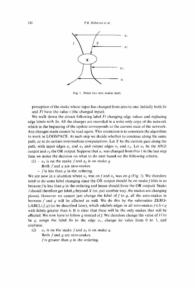
al
Fig. 1. When two zero snakes meet.
perception of the snake whose input has changed from zero to one. Initially both Sn
and Fl have the value i (the changed input).
We walk down the circuit following label F1 changing edge values and replacing
edge labels with Sn. All the changes are recorded in a write only copy of the network
which in the beginning of the update corresponds to the current state of the network.
Any changes made cannot be read again. This restriction is to constrain the algorithm
to work in LOGSPACE. At each step we decide whether to continue along the same
path, or to do certain intermediate computations. Let X be the current gate along the
path, with input edges a, and a2 and output edges oi and oz. Let o1 be the AND
output and o2 the OR output. Suppose that ai was changed from 0 to 1 in the last step
then we make the decision on what to do next based on the following criteria.
(1) ~ a, is on the snake f and a2 is on snake g.
~ Both f and g are zero-snakes.
- ,fis less than g in the ordering.
We are now in a situation where or was onfand o2 was on g (Fig. 1). We therefore
need to do some label changing since the OR output should be on snakef(this is so
becausefis less than g in the ordering and hence should force the OR output). Snake
fshould therefore get label g beyond X (or, put another way, the snakes are changing
pieces). However we cannot just change the label off to g, all the zero-snakes in
between f and g will be affected as well. We do this by the subroutine ZERO-
LABEL(f; g) (to be described later), which relabels edges in all zero-snakes f< h <g with labels greater than h. It is clear that these will be the only snakes that will be
affected. We now have to follow g instead off: We therefore change the value of Fl to
be g, assign the label Sn to the edge 02, change its value from 0 to 1, and
continue.
(2) - a1 is on the snake f and a2 is on snake g.
~ Both ,f and g are zero-snakes.
- f is greater than g in the ordering.
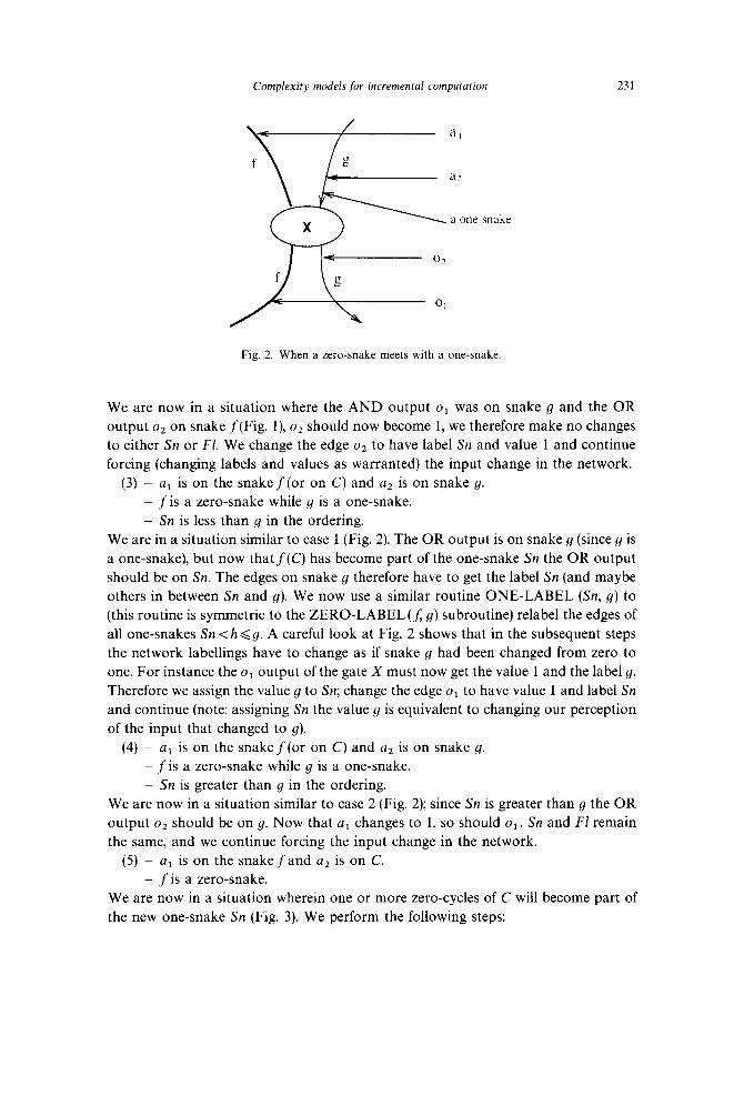
Complexity models for incremental computation 231
snake
Fig. 2. When a zero-snake meets with a one-snake.
We are now in a situation where the AND output or was on snake g and the OR
output o2 on snake f(Fig. l), o2 should now become 1, we therefore make no changes
to either Sn or FI. We change the edge o2 to have label Sn and value 1 and continue
forcing (changing labels and values as warranted) the input change in the network.
(3) - a, is on the snakef(or on C) and a2 is on snake g.
~ f is a zero-snake while g is a one-snake.
- Sn is less than g in the ordering.
We are in a situation similar to case 1 (Fig. 2). The OR output is on snake g (since g is
a one-snake), but now thatf(C) has become part of the one-snake Sn the OR output
should be on Sn. The edges on snake g therefore have to get the label Sn (and maybe
others in between Sn and g). We now use a similar routine ONE-LABEL (Sn, g) to
(this routine is symmetric to the ZERO-LABEL (f, g) subroutine) relabel the edges of
all one-snakes Sn < h d g. A careful look at Fig. 2 shows that in the subsequent steps
the network labellings have to change as if snake g had been changed from zero to
one. For instance the or output of the gate X must now get the value 1 and the label g.
Therefore we assign the value g to Sn; change the edge or to have value 1 and label Sn
and continue (note: assigning Sn the value g is equivalent to changing our perception
of the input that changed to g).
(4) ~ a, is on the snakef(or on C) and a2 is on snake g.
~ f is a zero-snake while g is a one-snake.
- Sn is greater than g in the ordering.
We are now in a situation similar to case 2 (Fig. 2); since Sn is greater than g the OR
output o2 should be on g. Now that a, changes to 1, so should or. Sn and Fl remain
the same, and we continue forcing the input change in the network.
(5) - a, is on the snakefand a2 is on C.
- f is a zero-snake.
We are now in a situation wherein one or more zero-cycles of C will become part of
the new one-snake Sn (Fig. 3). We perform the following steps:
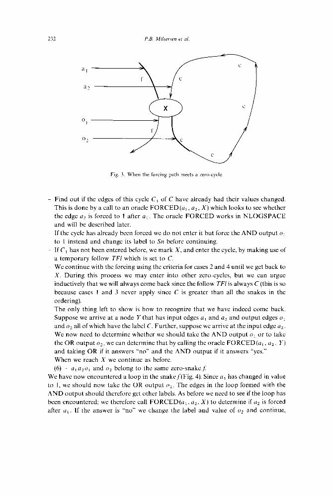
232
Fig. 3. When the forcing path meets a zero-cycle
- Find out if the edges of this cycle Cr of C have already had their values changed.
This is done by a call to an oracle FORCED(a,, a*, X) which looks to see whether
the edge u2 is forced to 1 after a1. The oracle FORCED works in NLOGSPACE
and will be described later.
~ If the cycle has already been forced we do not enter it but force the AND output or
to 1 instead and change its label to Sn before continuing.
- If Cr has not been entered before, we mark X, and enter the cycle, by making use of
a temporary follow TFl which is set to C.
~ We continue with the forcing using the criteria for cases 2 and 4 until we get back to
X. During this process we may enter into other zero-cycles, but we can argue
inductively that we will always come back since the follow TFl is always C (this is so
because cases 1 and 3 never apply since C is greater than all the snakes in the
ordering).
~ The only thing left to show is how to recognize that we have indeed come back.
Suppose we arrive at a node Y that has input edges al and a2 and output edges or
and o2 all of which have the label C. Further, suppose we arrive at the input edge a2.
We now need to determine whether we should take the AND output or or to take
the OR output ox, we can determine that by calling the oracle FORCED(a,, a2, Y)
and taking OR if it answers “no” and the AND output if it answers “yes.”
~ When we reach X we continue as before.
(6) - a, azo, and o2 belong to the same zero-snakef:
We have now encountered a loop in the snakef(Fig. 4). Since a1 has changed in value
to 1, we should now take the OR output oz. The edges in the loop formed with the
AND output should therefore get other labels. As before we need to see if the loop has
been encountered; we therefore call FORCED(ar, u2, X) to determine if u2 is forced
after u1 If the answer is “no” we change the label and value of o2 and continue,

Complexity models for incremental computation 233
f ,/- _-- ---------- --__
\ / -. \f / -1 \ \ \ 1’ f \ \ 1
(3 X
I I ‘\ f
f\
\ ‘.
I I.
I ’ ‘,
0
\
\f ; I \ I
Fig. 4. A self-loop that breaks up.
otherwise we perform the following steps to change the labels of the loop L consisting
of all the edges starting from o1 to a2 on the snakef: _ Change the labels of the edges in L to C (in the output tape). _ For all zero-snakes h >f(in the reverse order) find the earliest node Yin L such that
we can reach Y with a label h. Due to the change in snakefthe default labeling for
the edges in the loop L is C, however, if we can reach some node Yin L with some
label h (where h is a zero-snake), then some of the edges in L beyond Y would get the
label h (since C is greater than all the snakes in the ordering 7~). We therefore find the
earliest such Y by calling the routine REACHED( Y, h) (to be described later) for all
the Y’s one by one. Some of the ways a label h can reach the node Y are shown in
Figs. 4 and 5. In Fig. 4 we see the case wherein a subcycle of L gets the label h, and in
Fig. 5 we see how to reach Y with a label h after a complicated interchange of labels.
In this case all of L gets the label h. _ Label the edges in the smallest subcycle of L containing Y with label h.
The loop L has now been divided amongst the other snakes and C, note since we did
all the writes in the reverse order as in n we are guaranteed that the various orderings
will be obeyed at all nodes in the loop.
We now describe the subroutines FORCED, REACHED and ZERO-LABEL. The
procedure ONE-LABEL is similar to the ZERO-LABEL procedure and is omitted.
The procedure FORCED (a,, a*, Y) works as follows:
(1) Start at the input which has been changed and follow the path of forcing until
a node with a zero-cycle is reached. At this point we know that if we take the OR

234 P.B. Miltersen et al.
nodes where labels get interchanged
this sihlation occurs whenf<k<h
Fig. 5. How label interchanges affect the new labeling.
output we will come back; therefore we have a nondeterministic choice to make as to
whether we should take the OR or the AND output to reach the edge a2 of gate Y.
(2) If we reach a, first and then a2 within it steps we answer “yes” otherwise “no.”
The procedure REACHED( Y, h) works as follows:
(1) This procedure assumes that h is a zero-snake. We start at the input which has
been changed and follow the path of forcing until we encounter a zero-cycle or
a zero-snake g 3 h that is higher than or equal tof(the current F1) in the ordering. In
the former case we make a nondeterministic choice and follow one of the two outputs,
in the later case a nondeterministic choice is made to either continue with the forcing
(which means following snake g) entering the labeling phase.
(2) At the beginning of the labeling phase the followfl is set tofand the label I is set
to g if g ffand is set to C otherwise. We trace the snakefl till we meet a zero-snake gi
such that hdg, ~1. We now use nondeterminism again to decide which snake to
follow, if we followfl we change our current label 1 to gi, otherwise we changefl to be
equal to gi
(3) If we reach Y with label h in 2n steps we answer “yes,” otherwise we answer “no”.
The procedure ZERO-LABEL(5 g) works as follows:
(1) For all zero-snakes h, that f< h < g consider all the zero-snakes k # h and g in
the reverse order, and do the following:
(2) Find the earliest node Y on h with inputs a,, a2 and outputs or, o2 such that the
AND output o1 is on snake h, and Y can be reached with label k. This is done using the
subroutine REACHED.
(3) If such a Y exists relabel all the edges in h beyond Y with the label k.
Complexity models for incremental computation 235
An inductive proof can be used to show that ZERO-LABEL(i g) labels the snakes
f<h<g correctly. Note that all the changes are made on the write-only memory.
The proof of correctness of these procedures and the algorithm as a whole depends
upon the following crucial facts.
l While following snakefif we reach a node X such that a, is on the snakefand a2 is
on snake g, both f and g are zero-snakes, and f is less than g in the ordering, then
g has not been changed in any previous labeling.
l While following snake f if we reach a node X such that a, is on the snake f and a2 is
on snake g, f is a zero-snake while g is a one-snake, and the value of Sn is less than
g in the ordering, then g has not been changed in any previous labeling.
The proof follows from the fact that after every zero-labeling the value of Fl becomes greater than all the snakes whose edges have changed and after every
one-labeling the value of Sn becomes greater than all the snakes whose edges have
changed. This implies that even though we are allowed to look only at the input tape,
we have sufficient information to make correct decisions. In all our calls to NLOG-
SPACE oracles we have taken the liberty of assuming that the oracle gives both “yes”
and “no” answers accurately, which is not entirely correct. Every call to any of the
subroutines should be interpreted as a dual call to the routine and its complement
(executed in an interleaved fashion). When one of them answers we stop the other
routine, the whole computation is still in NLOGSPACE because NLOGSPACE and
CO-NLOGSPACE are the same [12]. Since the algorithm above works in LOG-
SPACE and uses NLOGSPACE oracles, the network-stability problem is in rincr-
LOGSPACE(NLOGSPACE).
Acknowledgments
We would like to thank the referees for pointing out the error in an earlier version of
the proof of Theorem 3.5 and for a number of other useful suggestions.
References
[l] D. Barrington, Bounded width polynomial size programs recognize exactly those languages in NC’,
in: Proc. 18th Symp. on Theory of Computing (1986) l-5. [2] A.M. Berman, MC. Paul1 and B.C. Ryder, Proving relative lower bounds for incremental algorithms,
Acta Inform. 27 (1990) 665-683. [3] R.B. Boppana and M. Sipser, The complexity of finite functions, in: Handbook of Theoretical Science
A (1990) 757-804. [4] A. Cook and P. Mckenzie, Problems complete for deterministic logarithmic space, J. Algorithms
8 (1987) 385-394. [S] A. Delcher and S. Kasif, Complexity issues in parallel logic programming, Ph.D. Thesis, Johns
Hopkins Univ., 1989.
163 S. Even and H. Gazit, Updating distances in dynamic graphs, Methods Oper. Res. 49 (1985) 371-387.
236 P.B. Miltersen et al.
[7] M.L. Fredman. Observations on the complexity of generating quasi-gray codes, SIAM J. Comput. 7 (1978) 134-146.
[S] M.L. Fredman, The complexity of maintaining an array and computing its partial sums, J. Assoc.
Comput. Mach. 29 (1982) 250-260.
[9] M.L. Fredman and M.E. Saks, The cell probe complexity of dynamic data structures, in: Proc. 2lsr
ACM Symp. on Theory of Computing (1989) 345-354. [lo] R. Greenlaw, H.J. Hoover and W.L. Ruzzo, A compendium of problems complete for P, Tech. Report
TR-91-05-01. Dept. of Computer Science and Engineering, Univ. of Washington, 1991.
[ll] L.J. Guibas and R. Sedgewick. A dichromatic framework for balanced trees, in: Proc. f9rh IEEE Symp. on Foundations qf Computer Science (1978) 8-21.
1121 N. Immerman, Nondeterministic Logspace is closed under complement, Tech. Report No
YALEEU/DCS/TR 552, Yale Univ., 1987.
1131 R.M. Karp and V. Ramachandran. A survey of parallel algorithms for shared memory machines, in:
J. van Leeuwen, ed., Handbook of Theoretical Cornpurer Science, Vol. A (Elsevier, Amsterdam. 1992)
871-941.
1141 R.E. Ladner, The circuit value problem is Log space complete for P, SIGACT New 7 (1975) 18-20. [15] E. Mayr and A. Subramanian, The complexity of circuit value and network stability, in: Proc. 4th Ann.
Conf: on Structure in Complexity Theory (1989) 114-123.
1161 K. Mehlhorn and M. Overmars, Optimal dynamiration of decomposable searching problems, Irt/brm. Process. Lett. 12 (1981) 93-98.
1171 P.B. Miltersen. On-line reevaluation of functions. Tech. Report ALCOM-91-63, Computer Science
Dept., Aarhus Univ., Aarhus DK., May 1991. [lS] S. Miyano, S. Shiraishi and T. Shoudai, A list of P-complete problems, Research Report, Research
Institute of Fundamental Information Science, Kyushu, Japan, 1989.
[19] M. Overmars, T/z Design qfDynamic Data Structures, Lecture Notes in Computer Science. Vol. 156
(Springer, Berlin, 1983).
[ZO] M.C. Paull, CC. Chang and A.M. Berman, Exploring the structure of incremental algorithms, Tech.
Report DCS-TR-139, Dept. of Computer Science, Rutgers Univ., May 1984.
[21] J.H. Reif, A topological approach to dynamic graph connectivity, Inform. Process. Left. 25 (1987) 65-70.
[22] S. Skyum and L.G. Valiant, A complexity theory based on boolean algebra, in: Proc. 22nd IEEE Symp. on Foundations oj’ Computer Science (198 1) 244-253.
1231 D.D. Sleator and R.E. Tarjan, A data structure for dynamic trees, J. Comptrt. Systems Sci. 24 (1983)
362-381. 1241 A. Subramanian. A new approach to stable matching problems, Tech. Report STAN-CS-89-1275.
Dept. of Computer Science. Stanford Univ., 1989.