complexity aspects of cooperative games - … · complexity aspects of cooperative games daniël...
TRANSCRIPT
Complexity Aspects of Cooperative Games
Daniël Paulusma
2001
Ph.D. thesisUniversity of Twente
Also available in print:www.tup.utwente.nl/uk/catalogue/technical/cooperative-games
T w e n t e U n i v e r s i t y P r e s s
Daniël PaulusmaComplexity Aspects of Cooperative Games

Publisher: Twente University Press, P.O. Box 217, 7500 AE Enschede, the Netherlands, www.tup.utwente.nl
Cover design: Jo Molenaar, [deel 4] ontwerpers, EnschedePrint: Grafisch Centrum Twente, Enschede
© D. Paulusma, Enschede, 2001
No part of this work may be reproduced by print, photocopy or any other means without the permission in writing from the publisher.
ISBN 9036515866
T w e n t e U n i v e r s i t y P r e s s

COMPLEXITY ASPECTS OF COOPERATIVE GAMES
PROEFSCHRIFT
ter verkrijging vande graad van doctor aan de Universiteit Twente,
op gezag van de rector magnificus,prof.dr. F.A. van Vught,
volgens besluit van het College voor Promotiesin het openbaar te verdedigen
op vrijdag 29 juni 2001 te 13.15 uur
door
Daniël Paulusmageboren op 23 mei 1974
te Leeuwarden
Dit proefschrift is goedgekeurd door de promotor
prof.dr. U. Faigle

Preface
This thesis is the result of the research that I started in June 1997 under super-vision of prof. U. Faigle. I want to thank him for the opportunity he offeredme, and I appreciated the cooperation with him.
Most of all I want to thank Walter Kern for his advice and support during theproject and the useful comments he gave on my thesis. I enjoyed workingwith him.
Next, I want to thank prof. J.M. Bilbao, prof. C. Hoede, prof. G. van der Laan,prof. S.H. Tijs and prof. G.J. Woeginger for taking place in my graduationcommittee.
Over the last years I was a member of the DOS department. I appreciatedthe nice working environment they offered, and I want to thank some of its(former) members in particular. Theo Driessen has taken a lot of interest inmy research and gave some useful comments on my thesis. Cindy Kuijpershelped me out many times, when I had a problem with Latex. I want tothank her and my other room-mates, Marcel Hunting and Petrica Pop, for thepleasant time I had with them.
Finally, I want to thank my family and friends for their support.
Daniel Paulusma Enschede, June 2001
v


Contents
Preface v
1 Introduction 11.1 Game theory . . . . . . . . . . . . . . . . . . . . . . . . . . . 11.2 Discrete optimization. . . . . . . . . . . . . . . . . . . . . . 31.3 Polyhedral theory . . . . . . . . . . . . . . . . . . . . . . . . 71.4 Graph theory . . . . . . . . . . . . . . . . . . . . . . . . . . 101.5 Outline of the thesis .. . . . . . . . . . . . . . . . . . . . . . 12
2 Solution concepts for cooperative games 152.1 Solution concepts: properties and complexity . . . . . . . . . 152.2 The core and least core . . . . . . . . . . . . . . . . . . . . . 182.3 The nucleolus . . . . . . . . . . . . . . . . . . . . . . . . . . 202.4 The f -least core andf -nucleolus . . . . . . . . . . . . . . . . 242.5 The Shapley value . . . . . . . . . . . . . . . . . . . . . . . . 31
3 Minimum cost spanning tree games 333.1 Introduction . . . . .. . . . . . . . . . . . . . . . . . . . . . 34
3.1.1 Minimum spanning trees .. . . . . . . . . . . . . . . 343.1.2 Minimum cost spanning tree games . . . . . .. . . . 36
3.2 The core of a minimum cost spanning tree game . . . . . . . . 373.3 The f -least core of a minimum cost spanning tree game . . . . 42
3.3.1 Introduction .. . . . . . . . . . . . . . . . . . . . . . 423.3.2 Minimum cover graphs . .. . . . . . . . . . . . . . . 453.3.3 Thef -least core of minimum cover graphs . . . . . . 473.3.4 Sufficient conditions forNP-hardness . . . . . . . . 52
vii

viii CONTENTS
4 Matching games 634.1 Matching theory . . . . . . . . . . . . . . . . . . . . . . . . . 634.2 Matching games in general . . . . . . . . . . . . . . . . . . . 70
4.2.1 Introduction .. . . . . . . . . . . . . . . . . . . . . . 704.2.2 Solution concepts for matching games . . . . .. . . . 72
4.3 Node matching games . . . . . . . . . . . . . . . . . . . . . . 774.3.1 The least core of node matching games . . . .. . . . 814.3.2 The nucleolus of node matching games . . . .. . . . 954.3.3 Cardinality matching games . . .. . . . . . . . . . . 99
5 Competition games 1015.1 Introduction . . . . .. . . . . . . . . . . . . . . . . . . . . . 1015.2 The sports competition problem .. . . . . . . . . . . . . . . 103
5.2.1 The model .. . . . . . . . . . . . . . . . . . . . . . 1035.2.2 Complexity results . . . .. . . . . . . . . . . . . . . 1065.2.3 Related problems . . . .. . . . . . . . . . . . . . . 114
5.3 Competition games .. . . . . . . . . . . . . . . . . . . . . . 116
Bibliography 121
Notations 127
Author Index 133
Subject Index 135
Summary 141
Samenvatting 143
About the author 145
Chapter 1
Introduction
Suppose a group of persons or organizations decide to work together in orderto make a profit on some market or to do an investment (building an electricitynetwork, constructing a railway etc.). Then the question arises how to split thejoint profit or cost. This allocation problem can be modeled and analyzed by(cooperative) game theory, which tries to come up with “fair” solutions (Sec-tion 1.1). This thesis studies several well-known allocation problems, wherethe cost or profit is computed as the optimal value of some discrete optimiza-tion problem. We are especially interested in the computational complexityof some frequently used solution concepts. Section 1.2 deals with complexitytheory and in Section 1.3 we treat some polyhedral theory. For readers notfamiliar with graph theory some basic terminology is included in Section 1.4.We end the chapter with an outline of the thesis.
1.1 Game theory
Game theory is a field of mathematical research that models and analyzes sit-uations of conflict. In such a situation, two or more individuals (theplayers)with similar or different interests are taking actions or making decisions. Thefoundations of game theory can be found in the paper of Von Neumann [1928]and the book “Theory of Games and Economic Behavior” by Von Neumannand Morgenstern [1944]. The situation of conflict first is described as a math-ematical model (thegame). One then uses mathematical solution methods tocome to a set of proposed pay-offs for each player. For a survey on gametheory we refer to the books of Owen [1995] and Shubik [1982].
1

2 Introduction
This thesis deals with so-called cooperative game theory, where players areallowed to cooperate with each other in order to optimize their profits (costs).
Definition 1.1 A cooperative game in characteristic function formis givenby an ordered pair.N; v/, whereN is a nonempty, finite set andv : 2N→R+is a function satisfyingv.∅/= 0. The setN is called theplayer setand itsn el-ements are theplayersof the game. The functionv is called thecharacteristicfunctionof the game. �
If a subset of players inN decide to work together, then they form acoalition.The mappingv assigns to each coalitionS⊆ N some outcomev.S/, thevalueor worthof coalitionS. v.S/ does not depend on the players outsideS. It canbe interpreted as the maximal profit or minimal cost that the players inScan achieve if they decide to form a coalition. In case of acost functionitis common to writec instead ofv. In the rest of this thesis we speak of a(cooperative) gameinstead of a cooperative game in characteristic functionform. In case of a profit functionv we may speak of aprofit gameand in caseof a cost functionc we may speak of acost game.
In cooperative game theory it is often assumed that the players decide to workall together. In that case thegrand coalition Nis formed. The central problemis to find a “fair” distribution of the total valuev.N/ among the individualplayersi ∈ N. Let xi denote the amount allocated to playeri ∈ N. A vectorx ∈ RN is anallocation if x is efficient, i.e., x.N/ = v.N/. (Throughout thethesis, we use the shorthand notationx.S/ =
∑i∈S
xi :)
A solution conceptprescribes for each game a set of allocations. In the liter-ature a solution concept can also assign pay-off vectors that are not efficient,but here we will assume that all vectors prescribed by some solution conceptare allocations.
The choice for a specific solution concept depends on the notion of “fairness”that has been specified within the decision model. Examples of solution con-cepts that might suggest more than one allocation are the core (Gillies [1959])and the kernel (Davis and Maschler [1965]). A solution concept that suggestsat most one allocation for each game is called avalue. Well-known values arethe Shapley value (Shapley [1953]) and the nucleolus (Schmeidler [1969]).
Example 1.1 Bankruptcy game(O’Neill [1982])Consider a situation where a company becomes a bankrupt and some cred-itors bring in a number of claims. The question here is how to divide the

1.2 Discrete optimization 3
available amount left by the company among the creditors. This situation canbe modeled as a cooperative game (N; v). N is the set of creditors and thecharacteristic functionv is given by
v.S/ :=max{0; E−∑
i∈N\Sdi} for all S⊆ N;
wheredi is the claim of creditori ∈ N andE<∑
i∈N di denotes the availableamount left by the company. A valuev.S/ can be interpreted as a lower boundof the amount that the players in a coalitionS⊆ N will receive if they do notprotest against the claims of players outsideS. A solution concept providesfor one or more possible distributions ofv.N/ = E among the creditors. �
1.2 Discrete optimization
In a generaldiscrete optimization problemwe have to optimize anobjectivefunction over a certain set called the(feasible) solution set. This set canbe described by (in)equality constraints and integrality restrictions on someor all of the variables. For a survey on discrete optimization we refer to thebooks of Nemhauser and Wolsey [1999], Papadimitriou and Steiglitz [1982]and Schrijver [1986].
An important aspect of a solution method for an optimization problem is itscomputational complexity. In this section we briefly go into the main con-cepts of complexity theory. More extended descriptions of these concepts canbe found in the books mentioned above and also in the book of Garey andJohnson [1979].
Assume that we have a solution setSand objective functionf : S→ R. Thenthe general optimization problem is
find a feasible solutions∈ Ssuch thatf .s/ = max{ f .s/ | s∈ S}:
The associateddecision problemis
Given f ∗ ∈ R; is there a solutions∈ Ssuch thatf .s/ ≥ f ∗?
So a decision problem is a question that has to be answered only by “yes” or“no”. Clearly, every solution method that solves the optimization problem canbe used to solve the associated decision problem. For adiscreteoptimization

4 Introduction
problem very often also the opposite is true: If one can solve the decisionproblem efficiently, then one can solve the corresponding optimization prob-lem efficiently. For this reason, the theory of complexity deals in the firstplace with decision problems.
An instanceof an optimization problem is a set of data that is obtained whenall the parameters that define the problem are fixed. Analgorithm is a listof instructions that solves every instance of a problem in a finite number ofsteps. So the output of an algorithm is “yes” in case there is a solution and“no” otherwise.
Example 1.2 EXACT 3-COVER (X3C)
Instance: A finite setW with 3q elements and a collectionU containingk≥ q3-element subsets ofW.
Question: DoesU contain anexact coverfor W, i.e., is there a subcollectionU ′ ⊆ U such that every element ofW occurs in exactly one member ofU′?
Determining the size of a minimum cover that contains every element ofW isthe associated (discrete) optimization problem. �
We assume that every instance is described as a string in a binary encoding.Thesize of a problem instanceis the length of the encoding, i.e., the numberof bits necessary to represent the instance. We denote the size of a rationalnumber a∈Q by< a>. For example, the size of a linear inequalityax≤ b,wherea andb are rational numbers, is equal to 1+ < a> + < b>, and thesize of a vectorx∈ Qn is equal ton+ < x1 > + < x2 > + : : :+ < xn >.
Because we want to obtain a general classification of problems, we assumethat every algorithm runs on the same machine, the so-called Turing machine,and we measure thecomputation timeof an algorithm by its number of per-formed elementary operations (additions, multiplications, comparisons etc.).
The running time t.¾/ of an algorithm is defined as the maximum (computa-tion) time required to solve any problem instance with size¾. In this way wehave an absolute guarantee on the time required to solve an instance indepen-dent of any probability distribution of the instances.
An algorithm is said to be apolynomial time algorithmor efficient if itsrunning timet.¾/ is bounded by a polynomial in¾, i.e, if for all ¾ ∈N; t.¾/=O.¾p/ for some fixedp∈ N. (For two functionsf : N→ R+ andg : N→ R+
1.2 Discrete optimization 5
we write f .n/ =O.g.n// if there exists positive numbersc;n0 ∈ N such thatf .n/ ≤ cg.n/ for n≥ n0.)
Decision problems that are solvable in polynomial time are considered to be“easy”. The class of these problems is denoted byP. P includes for exam-ple the minimum spanning tree problem and the weighted matching problem.Also several game theoretic problems such as computing the nucleolus of con-vex games (Kuipers [1996]) or computing the nucleolus of assignment games(Solymosi and Raghavan [1994]) can be solved efficiently.
An algorithm is said to be anexponential time algorithmif for all ¾ ∈N; t.¾/=O.2¾p
/ for some fixedp ∈ N. The class of decision problems solvable inexponential time is denoted byEX P. Most discrete optimization problemsbelong to this class.
If a problem is inEX P\P, then solving large instances of this problem willbe difficult. However, for a lot of problems it is not known whether they arein EX P\P or in P. X3C is an example of such a problem: No polynomialtime algorithm for X3C is known, and until so far X3C has not been provento be inEX P\P either. It is common believe that these kind of problems donot belong toP. Moreover, some of these problems can be considered to be“harder” than others. In order to make a more specific distinction the classesNP ⊆ EX PandNP-complete⊆ NP are introduced.
NP is the class of decision problems that can be solved by a so-callednon-deterministic algorithm. Such an algorithm consists of a guessing stage anda checking stage. In the first stage one guesses a solution and in the secondstage the algorithm checks if this solution satisfies the problem conditions. Ifthe checking stage can be done in polynomial time (with respect to the size ofthe instance in the guessing stage), then the problem is said to be inNP. X3Cis an example of a decision problem that is a member ofNP. A polynomialnondeterministic algorithm for X3C would be:
guessing stage: guess a subcollectionU ′ ⊆ U (of q elements).
checking stage: IfU ′ is an exact cover, then output “yes”;otherwise return.
ObviouslyP ⊆ NP holds. It is widely assumed thatP = NP is very un-likely. The classNP contains a subclass of problems that are considered tobe the hardest problems inNP. These problems are calledNP-complete
6 Introduction
problems. They have the following property: If one can prove that anNP-complete problem is a member ofP, thenP = NP holds. The techniqueused here is that of polynomially transforming one problem into another. Adecision problem51 is polynomially transformableto a decision problem52
if there exists an algorithm that for every instance¦1 of 51 produces inpoly-nomial timeexactly one instance¦2 of 52 such that the following holds:
the answer for¦1 is “yes” if and only if the answer of¦2 for “yes”.
This means that a polynomial time algorithmA for 52 can also be used tosolve an instance of51 efficiently: First polynomially transformate51 into52 and then useA.
Definition 1.2 A decision problem5 is calledNP-completeif 5 is inNPand all other decision problems inNP can be polynomially transformed to5. �
Note that polynomial transformability is a transitive relation. If51 is polyno-mially transformable to52 and52 is polynomially transformable to53, then51 is polynomially transformable to53. ClearlyP = NP must hold if onecan prove for anyNP-complete problem to be inP. If we want to prove thata decision problem5 isNP-complete, then we only have to show that
(i) 5 is inNP.
(ii) Some decision problem already known to beNP-complete can be poly-nomially transformed to5.
Our example X3C is one of the six basicNP-complete problems in Gareyand Johnson [1979]. The first problem proven to beNP-complete is the sat-isfiability problem (Cook [1971]). Other well-knownNP-complete problemsare the traveling salesman problem and Hamiltonian cycle. Some examplesof NP-complete problems in game theory are: deciding whether the core ofa minimum coloring game is empty or not (Deng, Ibaraki and Nagamochi[1999]) and testing membership in the core of minimum cost spanning treegames (Faigle, Kern, Fekete and Hochst¨attler [1997]).
Another technique that is used for proving that a problem can be solved inpolynomial time in case another problem can is polynomial reduction: Sup-pose we have two problems51 and52 not necessarily decision problems.

1.3 Polyhedral theory 7
A polynomial reductionfrom51 to52 is an algorithmA1 for 51 that usesan algorithmA2 for 52 as a subroutine and that would be a polynomial timealgorithm for51 if A2 were a polynomial time algorithm for52. This is amore general technique than polynomial transformation, which can be seenas a special case of reduction in which the subroutineA2 is used only once.
Definition 1.3 An optimization problem5 is calledNP-hard if there existsan N P-complete decision problem that can be polynomially reduced to5. �
Note that this definition includes all optimization problems for which the as-sociated decision problem isNP-complete. In particular, (the optimizationversion of) X3C isNP-hard. Polynomially reducibility is a transitive rela-tion. Therefore, in order to proveNP-hardness for some problem it sufficesto show that a knownNP-hard problem can be reduced to it. SomeNP-hardness results in game theory are computing the nucleolus of minimum costspanning tree games ( Faigle, Kern and Kuipers [1998a]) and computing theShapley value in weighted majority games (Deng and Papadimitriou [1994]).
1.3 Polyhedral theory
The theory we discuss in this section is derived from the the books of Schrijver[1986] and Gr¨otschel, Lovasz and Schrijver [1993].
Consider a set of pointsX = {x1; : : : ; xk} ⊆ Rn and a vector½ ∈ Rk. Thelinear combinationx =∑k
i=1½i xi is an affine combinationif∑k
i=1½i = 1,and x is called a convex combinationif besides
∑ki=1½i = 1; ½ ≥ 0. X is
called linearly (affinely) independentif no point xi ∈ X can be written as alinear (affine) combination of the other points inX.
A subsetS⊆ Rn is convexif for every finite number of pointsx1; : : : ; xk ∈ Sany convex combination of these points is a member ofS.
A nonempty setC⊆Rn is called aconvex coneif ½x+¼y∈C for all x; y∈Cand for all real numbers½;¼ ≥ 0.
A convex setP⊆ Rn is apolyhedronif there exists anm× n matrix A and avectorb∈ Rm such that
P= P.A;b/ = {x∈ Rn | Ax≤ b}:
We call Ax≤ b asystem of linear inequalities.

8 Introduction
A polyhedronP ⊆ Rn is boundedif there exist vectorsl ;u ∈ Rn such thatl ≤ x≤ u for all x∈ P. A bounded polyhedron is called apolytope.
For our purposes, only rational polyhedra are of interest. A polyhedron isrational if it is the solution set of a systemAx≤ b of linear inequalities, whereA andb are rational. A rational polyhedronP ⊆ Rn is said to havefacetcomplexity at most', if there exists a systemAx≤ b of linear inequalitieswith rational coefficients that hasP as its solution set and such that the sizeof each inequality of the system is at most'. From now on we will implicitlyassume a polyhedron to be rational.
A point x ∈ P is called avertexof P if x cannot be written as a convexcombination of other points inP. The following theorem presents a tightupper bound on the size of a vertex.
Theorem 1.1 Let P⊆ Rn be a polyhedron with facet complexity at most'.Then each vertex has size polynomially bounded byO.n2'/. �
Thedimensionof a polyhedronP⊆ Rn is equal to the maximum number ofaffinely independent points inP minus 1. An implicit equalityof the systemAx≤ b is an inequality
∑nj=1 aij xj ≤ bi of that system such that
∑nj=1 aij xj =
bi for all vectorsx ∈ P.A;b/. For Ax≤ b we denote the (sub)system ofimplicit equalities byA=x ≤ b=. Let rank(A) denote therank of a matrix,i.e., the maximum number of linearly independent row vectors. We have thefollowing standard result.
Theorem 1.2 The dimension of a polyhedron P.A;b/ ⊆ Rn is equal to n−rank.A=/. �
A subsetH ⊆ Rn is called ahyperplaneif there exists a vectorh ∈ Rn and anumberÞ ∈ R such that
H = {x∈ Rn | hTx= Þ}:A separating hyperplanefor a convex setSand vectorx =∈ S is a hyperplanegiven by a vectorh∈ Rn and a numberÞ ∈ R such thathTx≤ Þ andhT y> Þholds for ally∈ S.
Theseparation problemfor a polyhedronP⊆ Rn is, given a vectorx ∈ Rn,to decide whetherx∈ P or not, and, ifx =∈ P, to find a separating hyperplanefor P andx. A separation algorithmfor a polyhedronP is an algorithm thatsolves the separation problem forP.

1.3 Polyhedral theory 9
Linear programming(LP) deals with maximizing or minimizing a linear func-tion over a polyhedron. IfP⊆ Rn is a polyhedron andd ∈ Rn, then we callthe optimization problem
.LP/ max{dTx | x∈ P}
a linear program. A vectorx ∈ P is called a feasible solutionof the linearprogram andx∗ is called anoptimal solutionif x∗ is feasible anddTx∗ ≥ dTxfor all feasible solutionsx. If for all x ∈ P a solutionx∗ ∈ P exists withdTx∗ > dTx, then (LP) is unbounded. If ( LP) has no optimal solution then itis either infeasible or unbounded.
Khachiyan [1979] showed that LP can be solved in polynomial time by meansof the ellipsoid method. Gr¨otschel, Lovasz and Schrijver [1981] refined thismethod in such a way that the computational complexity of optimizing a linearfunction over a convex setS depends on the complexity of the separationproblem forS. If the convex set is a polyhedron, this can be stated as follows(see also Gr¨otschel, Lovasz and Schrijver [1993]):
Theorem 1.3 There exists an algorithm ELL and a polynomial p in two vari-ables n and' such that the following holds:
For each polyhedron P⊆ Rn with facet complexity at most' for which thereexists a separation algorithm SEP; ELL solves the linear program
max{dTx | x∈ P}
in time bounded by a polynomial in n; ';< d>; and T, where T is the maxi-mum time required by SEP on input vectors x of size p.n; '/. �
Here, “solving a linear program” not only means finding an optimal solution,but it also means detecting the cases in which the linear program is infeasibleor unbounded.
Now assume that for a polyhedronP ⊆ Rn with facet complexity at most' a separation algorithmSEPexists that solves on inputsx the separationproblem for P in time bounded by a polynomial inn; ' and< x >. Thenfrom Theorem 1.3 it follows immediately thatELL solves the linear programmax{dTx | x∈ P} in time bounded by a polynomial inn; '; and< d>.
Remark 1.1 For any polyhedronP, by definition, a linear systemAx≤ bexists such thatP= P.A;b/. In practice this description may be unknown

10 Introduction
or consists of too many inequalities. Theorem 1.3 shows that this is not aproblem as long as the facet complexity ofP is low and an efficient separationalgorithm for P is known. Moreover, in that case the running time ofELLonly depends on the size but not on the number of inequalities definingP. �
1.4 Graph theory
The games we study can be represented by graphs. We associate a cooper-ative game (N; v) with some graphG in the following way: The player setN is the node set ofG and the value of a coalitionv.S/ is determined as thevalue of a discrete optimization problem onG (e.g., the weight of a maxi-mum matching). In this section we include some terminology for readers notfamiliar with graph theory. For more on graph theory we refer to the book ofBondy and Murty [1976].
A graph Gis an ordered pair.V; E/, whereV is a nonempty, finite set calledthenode setandE is a set of (unordered) pairs (i; j) with i; j ∈ V called theedge set. If another graphG′ has been defined we writeG′.V/ andG′.E/ tomake a distinction.
The elements ofV are callednodesand the elements ofE are callededges. Ife= .i; j/ ∈ E we say that nodei and nodej are adjacent. In such a casei andj are called theend pointsof e or incidentwith e. Furthermore, we say thateis incidentwith i and j, and a subsetE′ ⊆ E of edges is said tocoverthe setof nodes incident with some edge inE′. A node j for which there is an edge.i; j/ ∈ E is aneighborof i. The number of neighbors of a nodei is calledthedegreeof i and denoted byŽ.i / and a node with no neighbors is called anisolated node. Two edges are calledadjacentif they have a common incidentnode.
A multigraphis a graph with possibly more than one edge between two nodes.
We speak of aweightedgraph if aweight functionw : E→ R is definedon the edge setE of a graphG. The numberw.e/ is theweightof an edgee∈ E. (It can usually be interpreted as a certain profit or cost.) Theweight ofa subset E′ ⊆ E is equal to the sum of the weights of its edges and denotedbyw.E′/.
A complete graphis a graph with an edge between every pair of nodes. Thecomplete graph onn nodes is denoted byKn.

1.4 Graph theory 11
A graphG is a bipartite graphwith node classes V1 andV2 if V = V1∪ V2;
V1∩ V2 = ∅ and each edge joins a node ofV1 to a node ofV2.
A subgraphof G is a graphG′ = .V′; E′/ with V′ ⊆ V and E′ ⊆ E. G′
is called the induced subgraph byV′, denoted byG|V′ , if E′ = {.i; j/ ∈E | i; j ∈ V′}. If V′ ⊆ V then we letG\V′ denote the graph obtained byremovingV′ (and the edges incident with nodes inV′). If E′ ⊆ E thenG\E′denotes the graph obtained by removing the edges inE′. We say that a graphG containsa graphG′ if G hasG′ as subgraph.
A path from i to j is a graphP = .V; E/ with a node set that can be or-dered asv0; : : : ; vn with v0 = i andvn = j such thatE = {.vk; vk+1/ | k =0; : : : ;n− 1}. The nodesi and j are called theend pointsof the path andnis thelengthof the path. We also writeP= v0v1 : : : vn.
A cycle is a graph for which the node set can be ordered asv0; : : : ; vn suchthat E= {.vk; vk+1/ | k= 0; : : : ;n− 1} ∪ {.vn; v0/}. We denote a cycle onn nodes byCn.
A graphG is called connectedif G contains a path fromi to j for each twonodesi; j ∈ V. A component G′ of G is a maximal connected subgraph ofG, i.e., if G is a connected subgraph ofG andG′ is a subgraph ofG, thenG= G′. Thesize of a componentis its number of nodes. We denote the sizeof a componentG′ by |G′|. A component is calledevenor odd if it has aneven respectively odd number of nodes.
A treeis a connected graphT that does not contain any cycle. A nodei ∈ V iscalled aleaf of a treeT = .V; E/, if i has exactly one neighbor. Aforestis agraph (not necessarily connected) that does not contain any cycle. Aspanningtreeof G= .V; E/ is a tree.V′; E′/ with V′ = V.
A matchingin a graphG= .V; E/ is a subsetM of E such that no two edgesin M have a common end point. A matchingM matchesa subsetV1 into V2,if each edge inM is incident with a node inV1 and a node inV2.
A node coverin a graphG= .V; E/ is a subsetV′ of V such that every edgein E is incident with a node inV′.
If the pairs.i; j/ in the edge set of a graph are ordered, then we speak of adirected graphor digraphand we call such an ordered pair.i; j/ an arc. Inthis case the edge set is usually denoted byA. If a= .i; j/ is an arc, then nodei is called the tail t.a/ of a and j is called thehead h.a/ of a. The arca isan outcoming arcof nodei and is anincoming arcof node j. Theoutdegree

12 Introduction
of a nodei, denoted byŽ+.i /, is the number of outcoming arcs ofi, and theindegreeŽ−.i / is the number of incoming arcs ofi.
A network.G; l ;u/ is a directed graphG = .V; A/ with two distinguishednodess andt and two functionsl : A→ R+ andu : A→ R+ such thatl .a/ ≤u.a/ for all a∈ A. s is called thesourceandt is called thesink. l is thelowercapacity functionandu is called theupper capacity function. l .a/ andu.a/are respectively thelower andupper capacityof arca∈ A.
A flow from s to t in a network.G; l ;u/ is a function f : A→ R such that forall i ∈ V\{s; t} ∑
t.a/=i
f .a/ =∑
h.a/=i
f .a/:
A flow f is called feasibleif for all a ∈ A l.a/ ≤ f .a/ ≤ u.a/. The fol-lowing standard result can be deduced from the Hoffman-Kruskal theorem(Hoffman and Kruskal [1956]).
Theorem 1.4 Let .G; l ;u/ be a network with integral capacities l and u.Then there exists an integral feasible flow for.G; l ;u/, if there exists a feasi-ble flow for.G; l ;u/. �
1.5 Outline of the thesis
The usefulness of a solution concept is not only determined by its modelingadequacy but also by its computational complexity. In this thesis we studythe complexity of several solution concepts with respect to various classes ofcooperative games.
In Chapter 2 we discuss a number of solution concepts for cooperative games,in particular the core and the nucleolus. Furthermore, we describe some leastcore concepts and variants of the nucleolus like the nucleon and the per-capitanucleolus.
Chapter 3 concentrates on minimum cost spanning tree games. Various leastcore concepts, including the classical least core, are analyzed. By a reductionfrom minimum cover problems we prove that computing an element in theseleast cores isNP-hard for minimum cost spanning tree games. As a conse-quence, computing the nucleolus, the nucleon and the per-capita nucleolus ofminimum cost spanning tree games is alsoNP-hard.

1.5 Outline of the thesis 13
Chapter 4 deals with matching games. In particular, we study cardinalitygames and a generalization thereof (node matching games). We show that thenucleolus and hence elements in the least core of such games can be computedefficiently. The case of general (weighted) matching games remains open.
In Chapter 5 we study complexity aspects of sports competitions like nationalfootball leagues and related games. The central problem is the so-calledelim-ination problem, i.e., to determine at a given intermediate state of the compe-tition whether a particular team still has a chance of winning the competition.Our main result states that the new FIFA-rules (3 : 0 for a win) have compli-cated this problem considerably. We completely characterize the complexityof this problem and relate it to the core complexity of a corresponding game.


Chapter 2
Solution concepts for cooperativegames
Recall that a solution concept8 prescribes a set8.N; v/⊆ RN of allocationsfor any cooperative game (N; v). In Section 2.1 we treat some elementaryproperties that a solution concept might have. The choice for a particularsolution concept depends on the “fairness” of its properties with respect tothe specific game one considers. We also make some general statements onthe computational complexity of solution concepts in this section. Section 2.2deals with the core and the least core of a game. The nucleolus is discussedin Section 2.3. In Section 2.4 we generalize the concepts of the previous twosections resulting in thef -least core and thef -nucleolus (special cases: thenucleon and the per-capita nucleolus). We end the chapter with a descriptionof the Shapley value of a game (Section 2.5).
2.1 Solution concepts: properties and complexity
Let (N; v) be a cooperative game. An allocationx ∈ RN is said to be animputationor individually rational if xi ≥ v.i / for all i ∈ N. An imputationallocates to each playeri ∈ N at least the amount thati can receive on hisown. Note that this definition is related to a profit game. In case of a costgame one has to reverse the inequalities (xi ≤ c.i /). The set of imputationsfor a game.N; v/ is denoted byI .N; v/.
I .N; v/ = {x∈ RN | x.N/ = v.N/ ; xi ≥ v.i / for all i ∈ N}:
15
16 Solution concepts for cooperative games
Obviously,I .N; v/ is nonempty if and only if∑
i∈N v.i / ≤ v.N/. The set ofallocations orpre-imputationsfor a game (N; v) is denoted byI ∗.N; v/.
I ∗.N; v/ = {x∈ RN | x.N/ = v.N/}:
In the rest of this chapter we mainly consider profit games, but the same the-ory can be applied to cost games. In that case some definitions have to beadjusted (more or less trivially by reversing some inequalities). In the lit-erature sometimes the notions anti-core and anti-nucleolus are used, if oneconsiders a cost game. Here we will still speak of the core and nucleolus of acost game.
Below we summarize a number of elementary properties or axioms for a solu-tion concept8 defined on a classG of cooperative games (see, e.g., Driessen[1991]). We use the following notations: IfX is a subset ofRN and½ ∈ R,then the set½X is equal to{½x | x∈ X}. If Y is also a subset ofRN, then thesetX+Y denotes the sum ofX andY, i.e., X+Y= {x+ y | x∈ X; y∈ Y}.
� Individual rationality (Ind)A solution concept8 is called individually rational if for all games.N; v/ ∈ G and allx∈ 8.N; v/ x is individually rational.
� Nonemptiness (Non)A solution concept8 has this property, if for all games (N; v/ ∈ G
8.N; v/ 6= ∅:
� Dummy player property (Dum)A player i ∈ N is called adummyin a game (N; v) if v.S/− v.S\i / =v.i / for all S⊆ N with i ∈ S. A solution concept8 has the dummyplayer property if for all games.N; v/ ∈ G, all dummy playersi ∈ N,and allx∈ 8.N; v/
xi = v.i /:
According to a solution concept that satisfiesDum, a dummy playerreceives exactly the amount that he contributes to every coalition.
� Symmetry (Sym)Let ³ : N → N be a permutation. The game (N; v³/ is given by

2.1 Solution concepts: properties and complexity 17
v³.³.S// = v.S/ for all S⊆ N. For any vectorx ∈ RN let the vec-tor x³ be given byx³³.i/ = xi for all i ∈ N. For any setX ⊆ RN; X³
defines the set
{y∈ RN | y= x³ for somex∈ X}:
A solution concept8 is symmetric if for all games (N; v/ ∈ G and allpermutations³ : N→ N
8.N; v³/ = 8.N; v/³:A symmetric solution concept is not influenced by renumbering of theplayer set.
� Invariance (Inv)Let .N; v/ ∈ G. Let ½ ∈ R anda∈ RN. The game (N; ½v+ a) is givenby .½v+ a/.S/= ½v.S/+ a.S/ for all S⊆ N. A solution concept8 iscalled invariant if for all games.N; v/ ∈ G, all ½ ∈ R, and alla ∈ RN
8.N; ½v+ a/ = ½8.N; v/+ {a}:
� Additivity (Add)Let .N; v/; .N; w/∈ G. The game (N; v+w) is given by.v+w/.S/=v.S/+w.S/ for all S⊆ N. A solution concept8 is additive if for allgames.N; v/ ∈ G and all.N; w/ ∈ G
8.N; v+w/ = 8.N; v/+8.N; w/:
A singleton is a set that contains exactly one element. In the previous chapterwe have stated that a solution concept that prescribes at most one allocationfor a game.N; v/ ∈ G is called a value. If a value8.N; v/ of a game (N; v)is nonempty, then we write, as a shorthand notation,8.N; v/ not only toindicate the singleton but also to indicate the allocation itself.
This thesis in particular studies classes of games, where each game (N; v)can be presented “implicitly” in terms of a(weighted) discrete structurefromwhich we can derive the coalition values. More precisely, (N; v) will be de-fined by a pair (G; w), whereG is a graph with node setV = N, andw is aweight function defined on the nodes and/or edges ofG. Given a coalitionS⊆ V we can computev.S/ by solving a (mostly easy) discrete optimizationproblem corresponding withS (cf. also Bilbao [2000]).

18 Solution concepts for cooperative games
Example 2.1 Let G = .N; E/ be a graph with node setN and edge setE.Letw : E→ R+ be a weight function defined onE. For S⊆ N we denote theset of edges joining nodes ofSby E.S/. We define a cooperative game (N; v)with characteristic functionv given by
v.S/ =∑
e∈E.S/
w.e/ for all S⊆ N:
�
We assume that thev-values we derive from the underlying discrete structure.G; w) have size polynomially bounded in the size of the structure. Henceto any game (N; v) in our class we may associate asize< N; v >, which ispolynomially bounded in the size of the underlying structure and at the sametime is an upper bound for the size of anyv-valuev.S/.
Example 2.2 In Example 2.1 we may define< N; v >= |N|2 < w >, where< w >=max{< w.e/ > | e∈ E}. �
Now consider an algorithmA that on input (N; v) (obtained from a discretestructure (G; w)) computes one or more allocations according to a solutionconcept8. ThenA is a polynomial time algorithm if its running time ispolynomially bounded in< N; v >.
2.2 The core and least core
Thecoreof a game is the most fundamental solution concept within coopera-tive game theory. The idea of the core essentially goes back to Von Neumannand Morgenstern [1944] and Ransmeier [1942]. The core was first introducedand named in Gillies [1959].
Definition 2.1 Thecoreof a game (N; v) is the following set of allocations:
core.N; v/ := {x∈ RN | x.N/ = v.N/; x.S/ ≥ v.S/ for all ∅ 6= S 6= N}:
�
A vector x ∈ core.N; v/ is said to be acore allocation. A core allocationxguarantees each coalitionS⊆ N to be satisfied in the sense that it gets at leastwhat it could gain on its own. As a solution concept the core satisfiesInd,SymandInv. Note that the core allocations form a polyhedron inRN.
2.2 The core and least core 19
A game (N; v) is called superadditiveif
v.S/+ v.T/ ≤ v.S∪ T/ for all S;T ⊆ N; S∩ T = ∅:In a superadditive game it is very likely that the grand coalitionN will beformed.
The following example shows that even for a superadditive three-person gamethe core can be empty. (Actually this is an example of a matching game onK3 with unit edge weights, cf. Chapter 4.)
Example 2.3 Consider the player setN = {1;2;3} and letv : 2N → R+ begiven byv.1/ = v.2/ = v.3/ = 0 andv.1;2/ = v.1;3/ = v.2;3/ = v.N/ =1. If x ∈ R3 were in the core, thenx1+ x2 ≥ 1 andx3 ≥ 0. Together withx.N/ = 1, this impliesx3 = 0. In the same way we can deducex1 = x2 = 0,a contradiction. Hence core(N; v) is empty. �
Because many interesting games, such as matching games, may have an emptycore, theadditivež-coreof a game (N; v) has been introduced (Shapley andShubik [1966]). For a givenž ∈ R, the additivež-core of (N; v) is the set ofallocations
{x∈ RN | x.N/ = v.N/; x.S/ ≥ v.S/+ ž for all ∅ 6= S 6= N}:
Obviously there exists anž ∈ R such that the additivež-core of (N; v) isnonempty. If we maximizež under the restriction thatž-core of (N; v) isnonempty, then we obtain theleast coreof a game (N; v) (Maschler, Pelegand Shapley [1979]).
Definition 2.2 The least coreof a game (N; v), denoted by leastcore(N; v),consists of all optimal solutionsx∈ RN of the linear program
.LC/ max ž
s:t: x.S/ ≥ v.S/+ ž .S 6= ∅; N/x.N/ = v.N/:
�
The least core of a game (N; v) tries to satisfy all coalitions∅ 6= S 6= N asmuch as possible. Adding all inequalitiesxi ≥ v.i /+ ž and usingx.N/ =v.N/ yields the upper bound
ž ≤v.N/−
∑i∈N v.i /
|N| :
20 Solution concepts for cooperative games
Hence (LC) has an optimal valuež∗ . Obviouslyž∗ ≥ 0 if and only if thecore of (N; v) is nonempty. Furthermore, if core(N; v) is nonempty thenleastcore(N; v) ⊆ core.N; v/.
The excessof a coalition∅ 6= S 6= N in a game (N; v) with respect to anallocationx∈ RN is defined as
e.S; x/ := x.S/− v.S/:
The excesse.S; x/ can be seen as a measure of satisfaction ofSwith respectto the allocationx. If e.S; x/ < e.T; x/ then coalitionSwill be less satisfiedwith allocationx than coalitionT.
Least core allocations are just those allocations that maximize the minimalexcessemin.x/ :=min{e.S; x/ | ∅ 6= S 6= N}:
leastcore.N; v/ = {x∈ RN | x.N/ = v.N/;emin.x/ = ž∗}:
2.3 The nucleolus
If the least core is not yet a single point, one might try to find “the best”allocation in the least core by further pursuing the idea of maximizing mini-mum excess: After satisfying the coalitions with the smallest excess as muchas possible, one tries to satisfy coalitions with the second smallest excess asmuch as possible and so on.
Given an allocationx ∈ RN, we define theexcess vector�.x/ ∈ R2N−2 byordering the 2N − 2 excess valuese.S; x/ in a non-decreasing sequence. Avectorx∈Rm is said to belexicographically smaller than or equal to y∈Rm,denoted byx� y, if x= y or there exists a number 1≤ j < n such thatxi = yi
if i ≤ j andxj+1 < yj+1.
Definition 2.3 Thenucleolusof a game (N; v) is the set of imputations{x ∈I .N; v/ | �.y/ � �.x/ for all y∈ I .N; v/}. �
Note that the nucleolus is the set of allocationsx∈ RN that lexicographicallymaximize�.x/ over I .N; v/. If the set of imputations is empty, then thenucleolus of (N; v) is the empty set. If we lexicographically maximize overthe whole set of allocationsI ∗.N; v/, we obtain theprenucleolusof (N; v).Both nucleolus and prenucleolus are defined as set valued solution concepts.However Schmeidler [1969] proved the following:

2.3 The nucleolus 21
Theorem 2.1 Let S⊆ RN be a nonempty convex set. Then the set{x ∈S | �.y/ � �.x/ for all y ∈ S} consists of exactly one point. �
From this result it follows that the nucleolus prescribes a unique allocation,if I .N; v/ is nonempty. In that case we denote the nucleolus of (N; v) by�.N; v/. By the same result also the prenucleolus, which exists for all games(N; v), is a singleton.
As a solution concept the nucleolus satisfiesInd, Dum, Symand Inv. Theprenucleolus only satisfies the last three properties.
It is immediately clear that computing the nucleolus by explicit lexicographicoptimization of the excess vector is not efficient: In general there are expo-nentially (in|N|) many different excess values, whereas an efficient procedureshould be polynomial in|N|. The standard procedure for computing the nu-cleolus proceeds by solving up to|N| linear programs (cf. Maschler, Pelegand Shapley [1979]). To present it we introduce the following notation: For apolyhedronP⊆ RN let
Fix P := {S⊆ N | x.S/ = y.S/ for all x; y ∈ P}
denote the set of coalitionsfixedby P. We assume thatI .N; v/ is nonemptyand letF0 := {∅; N}. First consider the linear program
.P1/ max ž
s:t: x.S/ ≥ v.S/+ ž .S =∈ F0/
x ∈ I .N; v/
with optimum valuež1 ∈ R. We let P1.ž/ denote the set of allx ∈ RN suchthat .x; ž/ satisfies the constraints of (P1). So core(N; v)= P1.0/. If ž1 ≥ 0,then leastcore(N; v/ = P1.ž1/.
Now, assume we have determinedP1.ž1/. We then proceed to maximize theminimal excess on those coalitions that are not already fixed, i.e., we solve
.P2/ max ž
s:t: x ∈ P1.ž1/
x.S/ ≥ v.S/+ ž .S =∈ Fix P1.ž1//:
Clearly (P2) is bounded and feasible. Hence letž2 > ž1 be the optimum valueof (P2). Extending our previous notation in the obvious way, we letP2.ž/

22 Solution concepts for cooperative games
denote the set of allx ∈ RN satisfying the constraints of (P2) for ž ∈ R. Nowproceed to
.P3/ max ž
s:t: x ∈ P2.ž2/
x.S/ ≥ v.S/+ ž .S =∈ Fix P2.ž2//
etc. until
.Pr / max ž
s:t: x ∈ Pr−1.žr−1/
x.S/ ≥ v.S/+ ž .S =∈ Fix Pr−1.žr−1//
defines a unique solutionx∗ ∈ RN, which is equal to�.N; v/, the nucleolusof the game. We have obtained this allocation after computing
ž1 < ž2 < : : : < žr
and P1.ž1/ ⊂ P2.ž2/ ⊂ : : : ⊂ Pr.žr / = �.N; v/.The same procedure can be applied to compute the prenucleolus, for whichwe only have to replace the constraintx ∈ I .N; v/ by x ∈ I ∗.N; v/ in thelinear program (P1). If core(N; v) is nonempty thenž1 ≥ 0 and in that casethe nucleolus and the prenucleolus coincide.
We see that in each iteration (implicit) equality constraints are added that areindependent of previous equality constraints. This implies that the feasibleregions of the above sequence of LP’s decrease in dimension. Hence we con-clude thatr ≤ |N|. So we compute at most|N| different excess values explic-itly. Note, however, that in each step we have to identify the setFix Pi.ži /.Furthermore, the number of constraints in each (Pi) remains exponential in|N|.The above “Linear Programming approach” to the nucleolus is also interest-ing from a structural point of view, as it implies a nice bound on the size< �.N; v/ > of the nucleolus.
Theorem 2.2 The nucleolus of a game (N; v) has size bounded polynomiallyin < N; v >.
Proof: LetF0⊂ : : :⊂Fr−1⊆ 2N denote the increasing sequence of fixed setsin .P1/; : : : ; .Pr /, i.e.,F0 = {∅; N} and
Fi := Fix Pi.ži / .i = 1; : : : ; r − 1/:

2.3 The nucleolus 23
Let the polyhedronP∗ ⊆ Rr+N be defined by
x.N/ = v.N/xi ≥ v.i / .i ∈ N/x.S/ ≥ v.S/+ ž1 .S =∈ F0/
x.S/ ≥ v.S/+ ž2 .S =∈ F1/...
x.S/ ≥ v.S/+ žr .S =∈ Fr−1/:
Then it is clear thatmax{ž1 |.ž; x/ ∈ P∗} yields ž1 = ž1,max{ž2 | .ž; x/ ∈ P∗; ž1 = ž1} yields ž2 = ž2 etc. untilmax{žr | .ž; x/ ∈ P∗; ž1= ž1; : : : ; žr−1= žr−1} has only one solution namely
.ž1; : : : ; žr; x∗/;
wherex∗ is the nucleolus of (N; v) andž1; : : : ; žr are the optimum values of.P1/; : : : ; .Pr /.
From the above it is straightforward to see that.ž1; : : : ; žr; x∗/ cannot bewritten as a convex combination of other points inP∗. Hence.ž1; : : : ; žr; x∗/is a vertex ofP∗. As such its size is polynomial in the dimensionr + |N| =O.|N|/ and the facet complexity (cf. Theorem 1.1). The latter is polynomiallybounded by< N; v >. �
Remark 2.1 From the proof of Theorem 2.2 it is also clear that the size ofthe parametersži .i = 1; : : : ; r / is polynomially bounded in< N; v >. �
So if we choose to compute the nucleolus of a game (N; v) by using thisalgorithmic procedure, then the only difficulties are
(i) identifying the setsFix Pi.ži / in each iteration step;
(ii) the exponential number of constraints in each (Pi).
In general these difficulties turn out to be hard. No polynomial time al-gorithms are known for computing the nucleolus in general. For instance,computing the nucleolus of minimum cost spanning tree games isNP-hard(Faigle, Kern and Kuipers [1998a]). Granot, Granot and Zhu [1998] study thecomplexity of the nucleolus in general. Several (not efficient) algorithms for

24 Solution concepts for cooperative games
computing the nucleolus in general have been developed (see, e.g., Potters,Reijnierse and Ansing [1996]). Positive results are known for some particularclasses of games. For instance, there exist efficient algorithms for comput-ing the nucleolus of standard tree games (Megiddo [1978], Granot, Maschler,Owen and Zhu [1996]), the nucleolus of convex games (Kuipers [1996]) andthe nucleolus of assignment games(Solymosi and Raghavan [1994]). Further-more, in Chapter 4 we will show that for a subclass of matching games we candescribe the polyhedra (Pi) by means of a polynomial number of inequalities.Also for this class of games the nucleolus can be computed efficiently.
2.4 The f -least core and f -nucleolus
In the literature, core relaxations different from the additivež-core have beenstudied. Faigle and Kern [1993] propose themultiplicativež-coreof a game(N; v). Here, thež-correction is directly related to the value v(S). For a givenž ∈ R, the multiplicativež-core of (N; v) is the set of allocations
{x∈ RN | x.N/ = v.N/; x.S/ ≥ v.S/+ žv.S/ for all ∅ 6= S 6= N}:
Also for the multiplicativež-core of aprofit game(N; v) there exists anž ∈ Rsuch that the multiplicativež-core is nonempty. For a cost game this doesnot need to be true. Consider for example a two-person game (N; c) withN = {1;2} andc given byc.1/ = c.2/ = 0 andc.N/ = 1. For allž ∈ R themultiplicativež-core is the set{x ∈ R2 | x1+ x2 = 1; x1; x2 ≤ 0}, which isempty.
The multiplicative least coreis defined in the same way as the classical leastcore, and we generalize as follows:
Definition 2.4 Let f : 2N → R+. Then the f -least coreof a game (N; v) isthe set of allocation vectors that are optimal solutions of the linear program
. f -LC/ max ž
s:t: x.S/ ≥ v.S/+ ž f .S/ .S 6= ∅; N/x.N/ = v.N/:
Denote this set byf -leastcore(N; v).
If ( f -LC) is unbounded, thenf -leastcore (N; v) is defined to be equal tocore(N; v). If ( f -LC) is infeasible, thenf -leastcore (N; v) is the empty set.
�
2.4 The f -least core andf -nucleolus 25
Obviously, the largerf .S/ is for some coalitionS⊂ N, the more decisiveSis for determining the optimum value of (f -LC). We therefore call a func-tion f as above apriority function. Note that f ≡ 1 corresponds with theclassical least core andf .S/ = v.S/ for all S⊆ N corresponds with the mul-tiplicative least core. In case of a cost game a priority functionf is closely re-lated to the concept of ataxation function: Shapley and Shubik [1966] definef .S/ = |S| for all S⊆ N and Tijs and Driessen [1986] propose theleast-taxcore, where f .S/ = v.S/−∑i∈Sv.i / for all S⊆ N. Note that for azero-normalizedgame(N; v) (a game wherev.i / = 0 for all playersi ∈ N) theleast-tax core of (N; v) is equivalent to the multiplicative least core of (N; v).
Motivated by the examples above (and also for computational reasons) wemainly restrict our attention to priority functionsf that satisfy the followingconditions:
(f1) f depends only on the size and the value of a coalition, i.e.,f is of thetype f : N×R→ R+. For∅ 6= S 6= N we set f .S/ = f .|S|; v.S//.
(f2) For all∅ 6= S 6= N; f .S/ can be computed in time bounded by a poly-nomial in< N; v >.
Because the empty coalition and the grand coalitionN have already fixed pay-offs, we can restrict a priority functionf : 2N→ R+ to the set 2N\{∅; N}.The next example shows that differentf -least cores can prescribe differentallocations. We compute the additive and multiplicative least core for a simpleclass of games.
Example 2.4 Suppose we have a situation where a number of persons wantto make a large profitv∗. They can only obtain this profit if they all make ajoint investment, where every personi invests an amountv.i /. We model thissituation by aninvestment game(N; v), wherev is given byv.S/ :=∑i∈Sv.i /for all S⊂ N andv.N/ = v∗ ≥∑i∈N v.i /. It is straightforward to check thatthe additive least core yields the unique allocationx∈ RN given by
xi = v.i /+v∗−
∑i∈N v.i /
|N| ;
while the multiplicative least core prescribes the unique allocationx ∈ RN
given by
xi = v∗ v.i /∑i∈N v.i /
:
26 Solution concepts for cooperative games
If players are payed according tox, then each player receives his own invest-ment plus an equal share of the amount that is left. If allocation vectorx isused, then they receive a pay-off relative to their investments. The last ruleseems to be more appropriate. In that case, for example, a playeri ∈ N withinvestmentv.i / = 0 is not paid anything. �
If f .S/ > 0 for some coalitionS⊂ N, then we have an upper bound
ž ≤ v.N/− v.S/− v.N\S/f .S/+ f .N\S/ :
Hence (f -LC) is unbounded if and only iff ≡ 0 on 2N\{∅; N}. Now as-sume (f -LC) to be feasible and bounded and letž∗f be the optimal value of( f -LC). Thenž∗f ≥ 0 if and only if core(N; v) is nonempty and the followingproposition is obvious.
Proposition 2.1 If core(N; v) 6= ∅, then
∅ 6= f -leastcore.N; v/ ⊆ core.N; v/ for all f : 2N→ R+:
�
We define thef -excessof a nonempty coalitionS⊂ N with respect to a vectorx∈ RN as the number
ef .S; x/ =
x.S/− v.S/
f .S/if f .S/ > 0
∞ if f .S/ = 0 andx.S/ ≥ v.S/−∞ otherwise:
Let efmin.x/ := min{ef .S; x/ | ∅ 6= S 6= N}. If ( f -LC) has an optimal value
ž∗f , then f -leastcore(N; v) can also be formulated as
f -leastcore.N; v/ = {x∈ RN | x.N/ = v.N/;efmin.x/ = ž∗f}:
In general, computing an allocation in thef -least core of a game (N; v) im-plies solving an exponential number of inequalities. However we can obtainthe following result (cf. also Faigle, Kern and Kuipers [1998b]).
Theorem 2.3 Let .N; v/ be a cooperative game, and f: 2N → R+ be a pri-ority function. Suppose that, for an allocation x∈ RN, a coalition∅ 6= S 6= N

2.4 The f -least core andf -nucleolus 27
with ef .S; x/ = efmin.x/ can be computed in time bounded by a polynomial
in < N; v > and< x >. Then an allocation in f -leastcore(N; v) can becomputed efficiently.
Proof: Let Pf ⊆ RN+1 denote the polyhedron of feasible solutions (x; ž) for( f -LC). We solve the separation problem forPf as follows: Given.x; ž/, wefirst check whetherx.N/ = v.N/ is satisfied. Next we compute a coalition∅ 6= S 6= N such thatef .S; x/= ef
min.x/. If efmin.x/≥ ž, then.x; ž/ is feasible.
If this is not true, our separating hyperplane is
{.x; ž/ ∈ RN+1 | x.S/− f .S/ž = v.S/}:By our assumption these computations can be done in time polynomiallybounded in< N; v > and< x >. Furthermore,Pf has facet complexity atmost< N; v > + < f >, where
< f >=max{< f .S/ > | ∅ 6= S 6= N}:By (f2),< f > is polynomially bounded in< N; v >. Then the result followsdirectly from Theorem 1.3. �
If the condition in Theorem 2.3 is satisfied, then we can compute the optimalvalue ž∗f of ( f -LC) in polynomial time. Ifž∗f is positive, then the core isnonempty. Otherwise the game (N; v) has an empty core. So, as a directconsequence of Theorem 2.3, we can efficiently check whether core(N; v) isempty or not.
Example 2.5 (see also Faigle, Kern and Kuipers [1998b]) Aconvex gameisa cost game (N; c) whose characteristic functionc is submodular, i.e.,
c.S∪ T/+ c.S∩ T/ ≤ c.S/+ c.T/ for all S;T ⊆ N:
Let f : 2N → R+ be a priority function. In case of a cost game thef -leastcore is defined as the set of optimal solutions of the linear program
. f -LC/ max ž
s:t: x.S/ ≤ c.S/− ž f .S/ .S 6= ∅; N/x.N/ = c.N/;
and thef -excess of a nonempty coalitionS⊂ N for a given vectorx∈ RN isgiven by
ef .S; x/ =
c.S/− x.S/
f .S/if f .S/ > 0
∞ if f .S/ = 0 andx.S/ ≤ c.S/−∞ otherwise:

28 Solution concepts for cooperative games
For f ≡ 1 it is straightforward to check that the excess function
e.:; x/ : 2N\{∅; N} → R
is also submodular. From a standard result in discrete optimization on min-imizing a submodular function (cf. Gr¨otschel, Lovasz and Schrijver [1993])it follows that computing a coalitionS such thate.S; x/ = emin.x/ can bedone in polynomial time. Hence, by Theorem 2.3 we conclude that we canefficiently compute an element in the least core of a convex game (N; c). �
Analogously to the introduction of thef -least core for a given priority func-tion f : 2N → R+ we can extend the notion of the classical nucleolus to thef -nucleolus. Order the 2N − 2 f -excess valuesef .S; x/ in a non-decreasingsequence resulting in thef -excess vector� f .x/. The f -nucleolusof (N; v)is then defined to be the set of all imputationsx ∈ RN that lexicographicallymaximize the excess vector� f .x/.
Definition 2.5 The f -nucleolusof a game (N; v) is the set of imputations{x∈ I .N; v/ | � f .y/ � � f .x/ for all y ∈ I .N; v/}. �
Note that thef -nucleolus for f ≡ 1 corresponds with the (classical) nucle-olus. In the literature the following examples have already been introduced:If f is given by f .S/ = v.S/ for all S⊂ N, then the f -nucleolus is calledthenucleon(Faigle, Kern, Fekete and Hochst¨attler [1998]). If f is given byf .S/ = |S| for all S⊂ N, then the f -nucleolus is called theper-capita nu-cleolus(see, e.g., Young, Okada and Hashimoto [1982]). Iff only dependson the size of a coalition, i.e.,f .S/ = f .T/ if |S| = |T| for all coalitionsS;T ⊂ N, then thef -nucleolus coincides with thef -nucleolus of Wallmeier[1983].
Contrary to the nucleolus, thef -nucleolus of a game (N; v) for some priorityfunction f 6≡ 1 does not necessarily consist of a single element. The followingexample illustrates this for the nucleon.
Example 2.6 Let .N; v/ be a two-person game, whereN = {1;2} andv isgiven byv.N/ = 1 andv.1/ = v.2/ = 0. Then the nucleon of.N; v/ is theset
{x∈ R2 | x1+ x2 = 1; x1; x2 ≥ 0}:
�

2.4 The f -least core andf -nucleolus 29
The algorithmic procedure for the nucleolus can also be applied to the generalf -nucleolus. We assumeI .N; v/ to be nonempty and letF0 := {∅; N}. For agiven priority function f : 2N→ R+ we consider the linear program
.Pf1 / max ž
s:t: x.S/ ≥ v.S/+ ž f .S/ .S =∈ F0/
x ∈ I .N; v/:
If ( Pf1 / has an empty feasible solution set, then thef -nucleolus of (N; v)
is empty. Otherwise letPf1 .ž/ denote the set of allx ∈ RN such that.x; ž/
satisfies the constraints of (Pf1 ). If .Pf
1 / is unbounded, thenf .S/ ≡ 0 andthe f -nucleolus of (N; v) is equal to core.N; v/. Otherwise letž f
1 ∈ R denotethe optimum value of.Pf
1 /. Note that core(N; v)= Pf1 .0/. Furthermore, if
core(N; v) is nonempty, thenž f1 ≥ 0; f -leastcore(N; v/= Pf
1 .žf1 / and, as we
shall see, thef -nucleolus of (N; v) is a subset of core(N; v).
In the next iteration we solve
.Pf2 / max ž
s:t: x ∈ Pf1 .ž
f1 /
x.S/ ≥ v.S/+ ž f .S/ .S =∈ Fix Pf1 .ž
f1 //:
If .Pf2 / is unbounded, then thef -nucleolus of (N; v) is equal toPf
1 .žf1 /. Oth-
erwise we have an optimal valuež f2 > ž
f1 and we proceed to
.Pf3 / max ž
s:t: x ∈ Pf2 .ž
f2 /
x.S/ ≥ v.S/+ ž f .S/ .S =∈ Fix Pf2 .ž
f2 //
etc. until
.Pfr+1/ max ž
s:t: x ∈ Pfr .ž
fr /
x.S/ ≥ v.S/+ ž f .S/ .S =∈ Fix Pfr .ž
fr //
is unbounded and thef -nucleolus of (N; v) is equal to the set
Pfr .ž
fr / . ⊂ Pf
r−1.žfr−1/ ⊂ : : : ⊂ Pf
1 .žf1 / /:
Note that in Example 2.4 it turns out that the nucleon of an investment game(N; v) is equal to its multiplicative least core, which contains exactly one allo-cation. However, Example 2.6 already shows that in general thef -nucleolus
30 Solution concepts for cooperative games
can consist of more than one vector. Obviously, thef -nucleolus of.N; v/ is aunique imputation if and only if{i} ∈ Fix Pf
r .žfr / for all i ∈ N. The following
proposition can be of importance for checking this condition.
Proposition 2.2 Let f : 2N → R+ be a priority function and let (N; v/ be agame with nonempty f -nucleolus. If f.S/ > 0 for a coalition∅ 6= S 6= N then,in some stage of the computation procedure for the f -nucleolus of (N; v/; Swill be fixed, i.e., S∈ Fix Pf
r .žfr / holds for some r> 0.
Proof: If .Pf1 / is unbounded thenf ≡ 0 holds. Assume that thef -nucleolus
of (N; v) is the setPfr .ž
fr / for somer > 0 andS =∈ Fix Pf
r .žfr / is a coalition
with f .S/ > 0. Let x be an imputation inPfr .ž
fr /. With respect to the linear
program.Pfr+1/ we have
v.N/ = x.N/ = x.S/+ x.N\S/ ≥ v.S/+ ž f .S/+ x.N\S/
implying an upper bound
ž ≤ v.N/− v.S/− x.N\S/f .S/
;
a contradiction. �
Corollary 2.1 Let f : 2N → R+ be a priority function with f.i / > 0 for alli ∈ N. If the f -nucleolus of a game (N; v) exists then it is a unique allocation.
�
Examples off -nucleoli satisfying this condition are the (classical) nucleolusand the per-capita nucleolus.
Corollary 2.2 Let f : 2N → R+ be a priority function with f.S/ = 0 if andonly if c.S/ = 0 for all S⊂ N and let.N; c/ be a cost game with c.N/ > 0.If the f -nucleolus of (N; c) exists then it is a unique allocation.
Proof: If .Pf1 / is unbounded thenf .S/ = 0 and thereforec.S/ = 0 for all
S⊂ N. Together withc.N/ > 0 this would imply that thef -nucleolus of(N; v) is empty.
Now assume that thef -nucleolus of (N; c) is a setPfr .ž
fr / containing more
than one vector. Then there exists a playeri ∈ N with {i} =∈ Fix Pfr .žr /. By
Proposition 2.2,c.i / = 0 must hold. Supposex ∈ Pfr .ž
fr /. If N\i is fixed by
Pfr .ž
fr / then, becausex.N/ = c.N/; {i} ∈ Fix Pf
r .žfr /, a contradiction. If

2.5 The Shapley value 31
N\i is not fixed then, again by Proposition 2.2,c.N\i / = 0. By our assump-tion also f .i / = f .N\i / = 0, and we have
c.N/ = xi + x.N\i /≤ c.i /− ž f
r f .i /+ c.N\i /− ž fr f .N\i /
= 0;
again a contradiction. �
By this result f -nucleoli, such as the nucleon and thef -nucleolus withf .S/=c.S/|S| for all ∅ 6= S 6= N, contain at most one allocation if they are applied to a
cost game.
2.5 The Shapley value
Recall that a value is a solution concept that prescribes at most one allocationfor every game (N; v). Shapley [1953] introduced the following value, whichis nonempty for any game (N; v).
Definition 2.6 The Shapley value�.N; v/ of a game.N; v/ is defined as
�i.N; v/ =∑
S⊆N\i
|S|!.|N| − |S| − 1/!|N|!
(v.S∪ i /− v.S/
)for all i ∈ N:
�
The Shapley value for a playeri can be interpreted as an expected allocation.If i joins a coalitionS, then this is rewarded with itsmarginal contributionv.S∪ i /− v.S/. The probability thati joins a coalition of size|S| is set to 1
|N|
for all sizes 0≤ |S| ≤ |N| − 1 and(|N|−1|S|)−1
for all coalitions of size|S|. This
results in a final probability equal to|S|!.|N|−|S|−1/!|N|! .
The Shapley value satisfiesNon, Sym, Dum, Add and Inv. Shapley [1953]even proved a stronger result.
Theorem 2.4 The Shapley value is the unique value that satisfies Sym, Dumand Add. �
32 Solution concepts for cooperative games
The Shapley value has been widely studied in the literature (see, e.g., Faigleand Kern [1992], Evans [1996], Driessen and Paulusma [2001], Sprumont[1990]). In general one has to compute all valuesv.S/ to obtain�.N; v/.Hence for most classes of games computing the Shapley value cannot be donein polynomial time.
The following example shows that�.N; v/ is not necessarily a core vector fora game (N; v).
Example 2.7 Consider a 3-person game (N; v), whereN = {1;2;3} andv isgiven by
v.1/ = 0 v.1;2/ = 2 v.N/ = 5:v.2/ = 0 v.1;3/ = 3v.3/ = 0 v.2;3/ = 4
Sincex ∈ R3 given byx1 = 0; x2 = 2 andx3 = 3 is easily seen to be a core-vector, core(N; v) is nonempty. Computing the Shapley value yields
�1.N; v/ = 76; �2.N; v/ = 10
6and �3.N; v/ = 13
6:
�.N; v/ is not in core(N; v), because coalition{2;3} receives236 , which is
less thanv.2;3/ = 4. �

Chapter 3
Minimum cost spanning treegames
In a minimum cost spanning tree game the players are represented by nodesin a complete graph and the cost of a coalition is equal to the weight of thecorresponding minimum spanning tree. In Section 3.1 we treat some basictheory on minimum spanning trees of a graph. Next we give the definition ofa minimum cost spanning tree game.
In Section 3.2 we discuss the core of a minimum cost spanning tree game.Granot and Huberman [1981] prove that these games have a nonempty coreby showing that certain vectors are core members. However, these allocationsmay not be acceptable from a modeling point of view, and Granot and Huber-man [1984] present some ways to construct other core allocations from thesevectors.
In Section 3.3 we study thef -least core of a minimum cost spanning treegame for various priority functionsf : 2N → R+. This is a more generalapproach than the approach followed by Granot and Huberman [1984]. Weprove that for a large class of priority functionsf computing an allocationin the f -least core of a general minimum cost spanning tree game isNP-hard. As a consequence also computingf -nucleoli, such as the nucleolus, thenucleon and the per-capita nucleolus of minimum cost spanning tree games,is in generalNP-hard.
33

34 Minimum cost spanning tree games
3.1 Introduction
3.1.1 Minimum spanning trees
Suppose an electricity network is to be built connecting a number of house-holds to a common power station. Installing an electricity cable between anytwo households and between any household and the power station is possible,but will cost a certain amount. Then the first task is to construct a networkthat connects every household to the power station and that has minimal cost.This example belongs to a class of problems where a number of users mustbe connected to a common supplier, and it can be modeled as a minimumspanning tree problem.
Definition 3.1 Let G= .V; E/ be a connected graph with a positive weightfunctionw ≥ 0 defined on the edge set E. Then a minimum spanning tree(MST) is a spanning tree T∗ of G that has minimal weight, i.e.,
w.E.T∗// = min{w.E.T// | T is a spanning tree of G}:
�
Computing an MST of a graphG= .V; E/ can be done in polynomial time by,for instance, the algorithm of Kruskal [1956] or the algorithm of Prim [1957].In the first algorithm an edge with minimal weight is chosen and afterwardsedges with weight as small as possible are added as long as no cycle occurs.In the end an MST has been constructed.
Algorithm of Kruskal
(1) SetE′ := ∅.(2) IF |E′| = |V| − 1 THEN outputT = .V; E′/. STOP.
(3) Choose an edgee′ ∈ E\E′ such that
w.e′/ =min{w.e/ | e∈ E\E′ and.V; E′ ∪ e/ does not contain a cycle}:
(4) SetE′ := E′ ∪ {e}. GOTO (2).

3.1 Introduction 35
The second algorithm starts with an arbitrary node inV. From this node itconstructs a tree with minimal weight that will be extended node by nodeuntil it spans the whole graph.
Algorithm of Prim :
(1) SetV′ := {v} for somev ∈ V and setE′ := ∅.(2) IF V′ = V THEN outputT = .V; E′/. STOP.
(3) Choose an edge.i; j/ ∈ E with i ∈ V′ and j ∈ V\V′ such that
w.i; j/ = min{w.k; l / | .k; l / ∈ E; k ∈ V′; l ∈ V\V′}:
(4) SetV′ := V′ ∪ { j} andE′ := E′ ∪ .i; j/. GOTO (2).
Example 3.1 Consider a complete graphG= .V; E/ on five nodes with weightfunction w : E → R+ as indicated in Figure 3.1. The treeT with edges
3
2 4
5
2
31
31
2
4
1
0
2
3
Figure 3.1
.0;1/; .1;3/; .1;4/ and.2;4/ and weightw.T/ = 7 is easily seen to be anMST of G. This MST is not unique: For instance, the treeT′ with edges.0;4/; .1;4/; .2;3/ and.2;4/ is also an MST ofG. �

36 Minimum cost spanning tree games
The following proposition (see, e.g., Aarts [1994]) shows that, given an MSTT of a graphG, each induced subgraph that is connected has an MST thatcontains all edges ofT with both end nodes in the induced subgraph.
Proposition 3.1 Let G= .V; E/ be a connected graph. Then for every MSTT of G and every set V′ ⊆ V, for which G|V′ is connected, an MST T′ of G|V′exists such that
E.T/∩ E.G|V′ / ⊆ E.T′/:
Proof: Use the algorithm of Kruskal to constructT. Suppose that in a certainstage of this algorithm the edgee′ ∈ E.T/ ∩ E.G|V′ / is added toE′. Sincew.e′/ =min{w.e/ | e∈ E\E′}, we have that
w.e′/ =min{w.e/ | e∈ E.G|V′ /\.E′ ∩ E.G|V′ //}:
Furthermore,.V; E′ ∪ e′/, and therefore.V′; .E′ ∩ E.G|V′ // ∪ e′/, does notcontain any cycle. This means that we can apply the algorithm of Kruskal forthe construction of an MSTT′ of G|V′ in such a way that we first choose theedges inE.T/ ∩ E.G|V′ /. �
3.1.2 Minimum cost spanning tree games
Consider again the example of an electricity network. After constructing anetwork that connects each user to the power station with minimum cost, thiscost has to be divided somehow among the users. Such an allocation problemcan be modeled as a minimum cost spanning tree game.
Definition 3.2 A minimum cost spanning tree game(MCST-game) (N; c) isdetermined by a setN of players, asupplynodes =∈ N, a complete graph withnode setV = N∪{s} and by a weight functionw ≥ 0 defined on its edge set.The costc.S/ of a coalitionS⊆ N is the weight of an MST in the subgraphinduced byS∪ {s}. �
In the definition above we see thatc.N/ is the weight of an MST in the orig-inal graph, which is exactly the minimum total cost of constructing the net-work. Because we only consider positive weight functionsw, for any MCST-game (N; c) we have
c.S/+ c.T/ ≥ c.S∪ T/ for all S;T ⊆ N; S∩ T = ∅:

3.2 The core of a minimum cost spanning tree game 37
So an MCST-game issubadditive, which makes the assumption that all play-ers decide to work together in order to divide the costc.N/ more likely.
The underlying discrete structure of an MCST-game (N; c) is a completegraphG and an edge weightingw. Let< w > denote the maximum size ofthe edge weights, i.e.,< w >:= max{< w.i; j/ >}. We define< N; c >=|N| < w >.
A basic observation is now the following. If a nodei ∈ N occurs as a leaf insome MSTT for G and if e is the unique edge inT incident withi, thenT\eis an MST for the subgraph induced byV\i. So in this case we immediatelydeduce that
c.N\i / = c.N/−w.e/: (3.1)
Example 3.2 Consider again the graphG in Example 3.1. If we assume node0 to be the supply node then we obtain an MCST-game (N; c), whereN ={1;2;3;4} andc : 2N→ R+ is given by
c.1/ = 2 c.1;2/ = 4 c.1;2;3/ = 7 c.N/ = 7:c.2/ = 3 c.1;3/ = 5 c.1;2;4/ = 4c.3/ = 4 c.1;4/ = 3 c.1;3;4/ = 6c.4/ = 2 c.2;3/ = 6 c.2;3;4/ = 6
c.2;4/ = 4c.3;4/ = 6
�
3.2 The core of a minimum cost spanning treegame
Minimum cost spanning tree problems have been widely studied in the lit-erature. After their introduction by Bird [1976], various results about thecore and nucleolus were established (see, e.g., Aarts [1994], Faigle, Kern andKuipers [1998a], Granot and Huberman [1981], [1984]).
Granot and Huberman [1981] proved the following theorem, which shows thatany MCST-game has a nonempty core and that a core allocation can be foundin polynomial time. A core allocation as defined below is called astandardcore allocation. We denote the standard core allocation corresponding to anMST T∗ by x∗.

38 Minimum cost spanning tree games
Theorem 3.1 Let T∗ be a minimum spanning tree belonging to an MCST-game (N; c). Then the vector x∗ ∈ RN that allocates to player i∈ N theweight of the first edge i encounters on the (unique) path from i to s in T∗ is avertex of core(N; c). �
However, Granot and Huberman [1981] also point out that standard core allo-cations may not be acceptable from a modeling point of view. The followingexample illustrates this.
Example 3.3 Consider an MCST-game (N; c) obtained from a complete graphG on four nodes with edge weightingw as indicated in Figure 3.2. Clearly,
10
1 1
11 11
1
s
3 2
1
Figure 3.2
the treeT∗ with edges.s;1/; .1;2/ and.1;3/ and weightw.T∗/ = 12 is anMST of G. The corresponding standard core allocationx∗ is given byx∗1 = 10andx∗2 = x∗3 = 1. So most of the cost is charged to player 1, although player2 and 3 highly depend on this player for their connection tos. This motivatesthe search for other core allocations such as the vectorx given byx1 = 2 andx2 = x3 = 5. �
The question arises how to find possibly more appropriate core allocationsand what is the computational complexity of computing these allocations.
Granot and Huberman [1984] propose the following procedure to obtain coreallocations not equal to a standard core allocation: LetT∗ be a minimum

3.2 The core of a minimum cost spanning tree game 39
spanning tree belonging to an MCST-game (N; c) determined by a completegraphG with node setV = N∪{s} and edge weightingw. Supposei is not aleaf of T∗. Let Fi.T∗/ denote the set ofimmediate followersof nodei in T∗,i.e.,
Fi.T∗/ = { j ∈ N | i is the 1st nodej encounters on the path fromj to s in T∗}:
For all core allocationsx we havex.N/ = c.N/ andx.N\i /≤ c.N\i /. Theseconstraints imply that according tox∗ ∈ core(N; c) at least an amount of
c.N/− c.N\i /
is charged to nodei. If x∗i > c.N/− c.N\i / then one could try to modify thestandard core allocationx∗ such that nodei pays less, while the immediatefollowers of i are charged a higher amount for their connection tos via i.For this purpose, Granot and Huberman [1984] introduced the so-calledweakdemand operation. This operation can be applied on an arbitrary allocationx ∈ RN, but here we show only its effect on standard core allocations. Forthose allocations the method transfers an amount fromi to Fi.T∗/ in sucha way that the resulting vector is still a core vector and playeri is chargedexactlyc.N/− c.N\i /.In order to explain the method we have to use Proposition 3.1. By this propo-sition, there exists an MSTT′ of the subgraph ofG induced byN\i suchthat
E.T∗/∩ E.G|N\i/ ⊆ E.T′/: (3.2)
For eachj ∈ Fi.T∗/ there exists an edgeej that is the first edgej encounterson the unique path fromj to s in T′ that is not an edge inT∗. Then the weakdemand operation applied inT∗ by i on x∗ with respect toT′ yields the vectorx∈ RN given by
x j =
c.N/− c.N\i / if j = iw.ej / if j ∈ Fi.T∗/x∗j otherwise.
The example below shows that in caseT′ is not the unique tree satisfying (3.2)the weak demand operation can yield a different vector.
Example 3.4 Let (N; c) be an MCST-game (N; c) obtained from a completegraphG on five nodes with edge weightingw as indicated in Figure 3.3. The

40 Minimum cost spanning tree games
4 9
3
1 4
19
21
91
s
2
34
Figure 3.3
treeT∗ with edges.s;1/; .1;3/; .1;4/ and.2;3/ is an MST ofG with weightw.T∗/ = 5. Thenc.N/ = 5 andx∗ ∈ R4 is the vector.1;2;1;1/.
Node 1 is not a leaf ofT∗ and its set of immediate followersF1.T∗/ is equalto {3;4}. The treeT′ with edges.s;2/; .2;3/ and.3;4/ is an MST ofG|N\1with weightw.T′/ = 9. Soc.N\1/ = 9. The weak demand operation by 1on x∗ with respect toT′ yields the allocationx1 = .−4;2;4;3/. Also the treeT′′ with edges.s;4/; .2;3/ and .3;4/ is an MST ofG|N\1 satisfying (3.2).Applying the weak demand operation with respect toT′′ yields the allocationx2 = .−4;2;3;4/. �
Note that in Example 3.4 bothx1 and x2 are core allocations. The followingresult by Granot and Huberman [1984] states that this holds for all vectors ob-tained after applying a weak demand operation on a standard core allocation.
Theorem 3.2 Let T∗ be an MST belonging to an MCST-game (N; c/ deter-mined by a complete graph G with edge weightingw. Let i∈ N, and let T′ bean MST of GN\i such that
E.T∗/∩ E.G|N\i/ ⊆ E.T′/:
Then the vectorx ∈ RN obtained by the weak demand operation applied inT∗ by i on x∗ with respect to T′ is an element in core(N; c). �
3.2 The core of a minimum cost spanning tree game 41
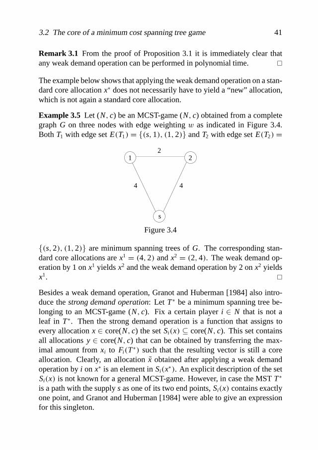
Remark 3.1 From the proof of Proposition 3.1 it is immediately clear thatany weak demand operation can be performed in polynomial time. �
The example below shows that applying the weak demand operation on a stan-dard core allocationx∗ does not necessarily have to yield a “new” allocation,which is not again a standard core allocation.
Example 3.5 Let (N; c) be an MCST-game (N; c) obtained from a completegraphG on three nodes with edge weightingw as indicated in Figure 3.4.Both T1 with edge setE.T1/ = {.s;1/; .1;2/} andT2 with edge setE.T2/ =
4 4
21 2
s
Figure 3.4
{.s;2/; .1;2/} are minimum spanning trees ofG. The corresponding stan-dard core allocations arex1 = .4;2/ andx2 = .2;4/. The weak demand op-eration by 1 onx1 yieldsx2 and the weak demand operation by 2 onx2 yieldsx1. �
Besides a weak demand operation, Granot and Huberman [1984] also intro-duce thestrong demand operation: Let T∗ be a minimum spanning tree be-longing to an MCST-game (N; c). Fix a certain playeri ∈ N that is not aleaf in T∗. Then the strong demand operation is a function that assigns toevery allocationx ∈ core(N; c) the setSi.x/ ⊆ core(N; c). This set containsall allocationsy ∈ core(N; c) that can be obtained by transferring the max-imal amount fromxi to Fi.T∗/ such that the resulting vector is still a coreallocation. Clearly, an allocationx obtained after applying a weak demandoperation byi on x∗ is an element inSi.x∗/. An explicit description of the setSi.x/ is not known for a general MCST-game. However, in case the MSTT∗
is a path with the supplys as one of its two end points,Si.x/ contains exactlyone point, and Granot and Huberman [1984] were able to give an expressionfor this singleton.

42 Minimum cost spanning tree games
3.3 The f -least core of a minimum cost spanningtree game
3.3.1 Introduction
In the previous section only new core allocations were obtained from standardcore allocations by transferring a certain amount from one fixed player toits set of immediate followers. Here we follow a more general approach byconsidering thef -least core of an MCST-game (N; c) for a number of priorityfunctions f 6≡ 0. Recall that thef -least core of a cost game (N; c) is the setof allocation vectors that are optimal solutions of the linear program
. f -LC/ max ž
s:t: x.S/ ≤ c.S/− ž f .S/ .S 6= ∅; N/x.N/ = c.N/:
Since core(N; c) is nonempty, by Proposition 2.1 thef -least core of an arbi-trary priority function f is a nonempty subset of core(N; c).
We are interested in the computational complexity of computing an element inthe f -least core for a priority functionf . First we show that this approach canbe seen as a generalization of the methods described in the previous section.
Let .N; c/ be an MCST-game. Assume that a playeri ∈ N is more importantthan the other players, for instance, by its position in the network. We canexpress this by a priority functionf i : 2N→ R+ given by
f i.S/ ={
1 if S= {i}0 otherwise.
The following proposition gives a characterization of thef i-least core of anMCST-game.
Proposition 3.2 Let .N; c) be an MCST-game and i∈ N. Then
f i-leastcore.N; c/ = core.N; c/∩ {x∈ RN | xi = c.N/− c.N\i /}:
Proof: Supposex ∈ f i-leastcore(N; c). The feasibility constraintsx.N/ =c.N/; x.N\i / ≤ c.N\i / together withxi ≤ c.i /− ž yield the upper bound
ž ≤ c.i /+ c.N\i /− c.N/:

3.3 The f -least core of a minimum cost spanning tree game 43
Let ž∗ = c.i /+ c.N\i /− c.N/. Thenž∗ is the optimal value of. f i-LC/, ifwe can show that a feasible solution.x; ž∗/ of . f i-LC/ exists.
Now let T∗ be an MST belonging to (N; c). If x∗i = c.N/− c.N\i / we havex∗i = c.i /− ž∗ and, sincex∗ ∈ core(N; c), x∗.S/≤ c.S/ for all S⊂ N. Other-wise the vectorx obtained after applying a weak demand operation by playeri in T∗ on x∗ satisfiesxi = c.N/− c.N\i / = c.i /− ž∗, and by Theorem 3.2x is a member of core(N; c), and thusx.S/ ≤ c.S/ for all S⊂ N. Hencež∗ isthe optimal value of. f i-LC/.
Note thatž∗ ≥ 0. By the feasibility constraints of. f i-LC/ an allocationx isan element inf i-leastcore(N; c) if and only if
xi = c.N/− c.N\i / and x.S/ ≤ c.S/ for all ∅ 6= S 6= N;
which proves the proposition. �
From the proof of Proposition 3.2 it is clear thatSi.x∗/ ⊆ f i-leastcore(N; c)for any MSTT∗ belonging to (N; c). In particular an allocationx ∈ RN ob-tained after applying a weak demand operation byi on x∗ is an element off i-leastcore(N; c). Because such a vector can be computed efficiently (cf.Remark 3.1), the following corollary holds.
Corollary 3.1 Let (N; c) be an MCST-game and i∈ N. Then computing anelement in fi-leastcore(N; c) can be done in polynomial time. �
In the following we will introduce a class of priority functions for which com-puting the f -nucleolus isNP-hard. This class contains both the nucleolusand the nucleon. Below we give an example in which the nucleolus and thenucleon are computed.
Example 3.6 Consider an MCST-game (N; c) obtained from a complete graphG = .V; E/ on three nodes and edge weights as defined in Figure 3.5. Thetree T∗ with edges.s;1/ and .1;2/ is an MST ofG and the standard coreallocationx∗ is given byx∗1 = 10 andx∗2 = 1, which may be considered to beunfair with respect to player 1. Solving the linear program
max ž
s:t: x1+ x2 = 11x1 ≤ 10− žx2 ≤ 11− ž

44 Minimum cost spanning tree games
1
11
10
s
2
1
Figure 3.5
yields the unique (additive) least core allocationx given byx1= 5 andx2= 6.Solving the linear program
max ž
s:t: x1+ x2 = 11x1 ≤ 10− 10žx2 ≤ 11− 11ž
yields the unique multiplicative least core allocationy given byy1 = 5 521 and
y2 = 51621. �
In Example 3.3 both the additive and multiplicative least core are equal to thesingleton{.0;6;6/}.The rest of this chapter is based on Faigle, Kern and Paulusma [2000]. Wewill define a class of priority functions, for which computing an element inthe f -least core of an MCST-game (N; c) turns out to beNP-hard. This classcontains priority functionsf such as
� f .S/ = 1 for all ∅ 6= S 6= N� f .S/ = c.S/ for all ∅ 6= S 6= N� f .S/ = |S| for all ∅ 6= S 6= N:
The proof uses a reduction from minimum cover problems. We show thatcomputing a least core allocation for a special class of graphs introduced in

3.3 The f -least core of a minimum cost spanning tree game 45
Faigle, Kern, Fekete and Hochst¨attler [1997] is alreadyNP-hard. Thesegraphs will be treated in Section 3.3.2. Section 3.3.3 contains the proof ofthe theorem. In Section 3.3.4 the functions mentioned above are treated. Bygiving sufficient conditions for a priority functionf to satisfy a number ofproperties defined in Section 3.3.3, we prove that computing an element inthe f -least core of MCST-games isNP-hard for these functions. Megiddo[1978] and Granot, Maschler, Owen and Zhu [1996] give a polynomial al-gorithm for computing the nucleolus in case the underlying graph is not acomplete graph but a tree. Faigle, Kern and Kuipers [1998a] show that com-puting the nucleolus of a general MCST-game isNP-hard. Here we obtainthis result as an immediate corollary from our main theorem. Also, as a con-sequence of this result, computing the nucleon and the per-capita nucleolus ofMCST-games is in generalNP-hard.
3.3.2 Minimum cover graphs
In this section we define a minimum cover graph and we show how we canconstruct an MCST-game from such a graph.
Let q∈ N, and letU be a set ofk≥ q elements andW be a set of 3q elements.
Consider a bipartite graph with node setU ∪W (partitioned intoU andW)such that each nodeu ∈ U is adjacent to exactly three nodes inW. We saythat nodeu ∈ U coversits three neighbors inW.
A set D ⊆ U is called acover if eachw ∈ W is incident with someu ∈ D.A minimum coveris a cover that minimizes|D|. Finding a minimum coveris a well-knownNP-hard problem. It includes theNP-complete problemX3C (cf. Example 1.2). Below we show that we may restrict ourselves to asubclass of minimum cover problems.
Proposition 3.3 Finding a minimum cover under the following assumptionsisNP-hard.
(C1) Each node in W has degree 2 or more.
(C2) The size of a minimum cover is at most q+ 2.
Proof: Supposew ∈W is a node with degree 1,w is connected tou andu isalso connected tow1 andw2. Add a nodeu to U and connect it tow, w1 andw2. The size of a minimum cover will not change. Hence computing the size

46 Minimum cost spanning tree games
of a minimum cover, in case (C1) holds, is at least as hard as computing thesize of a minimum cover in the general case.
To show the validity of (C2), add nodesu1;u2; : : : ;uq to U that coverW.Eachui .i = 1; : : : ;q/ covers exactly 3 nodes inW. Next deleteuq. The sizeof a minimum cover will be less than or equal toq+ 2. If the size is greaterthanq, the original problem has no exact cover. If the size of a minimumcover is equal toq, then also deleteuq−1. Again the size of a minimum coverwill be at mostq+ 2. If the size is greater thanq, the original problem hasno exact cover. If the size is equal toq, also deleteuq−2 and so on. In eachstep of the procedure only problems that have a minimum cover with size atmostq+ 2 are considered. Ifu1 would be deleted, one arrives at the originalproblem. Hence computing the size of a minimum cover, in case (C2) holds,is at least as hard as computing the size of a minimum cover in the generalcase. �
From now on we assume that conditions (C1) and (C2) hold. We constructan MCST-game from a minimum cover problem as follows (cf. Faigle, Kern,Fekete and Hochst¨attler [1997]). First we define aminimum cover graph G=.V; E/. The node set ofG consists ofU ∪W and three additional nodes:TheSteiner node St, theguardian gand the supplys. The edge setE of Gcomprises the following (cf. Figure 3.6).
� all edgese from the bipartite graph onU ∪W, each of them havingweightw.e/ = q+ 1;
� for eachu∈U, an edge.u; St/ betweenuandStwith weightw.u; St/=q and an edge.u; g/ betweenu andg with weightw.u; g/ = q+ 1;
� an edge.St; g/ betweenStandg with weightw.St; g/ = q+ 1;
� an edge.g; s/ betweeng ands with weightw.g; s/ = 2q− 1.
We extendG to the complete graphG on V with weights induced fromG,i.e., if e= .i; j/ is an edge inG, thenw.i; j/ is the weight of a shortest pathfrom i to j in G.
An MST in G is obtained by connecting eachw ∈W to someu∈U by whichit is covered. Such au ∈ U exists because each nodew ∈ W has a neighborin U (indeed, it has at least 2 neighbors inU). Then one connects eachu∈ U

3.3 The f -least core of a minimum cost spanning tree game 47
q+1
W
U
g
s
St
q+1
q
...
...
...
2q−1
q+1
Figure 3.6. a minimum cover graph
to St, and finally connectsSt to g andg to s. The resulting MST has a totalweight of
c.N/ = 3q.q+ 1/+ kq+ 3q:
Furthermore, by (C1), eachw ∈ W is covered by at leasttwo nodes inU.Hence it is straightforward to see that the following property holds forG:
(L ) For eachv ∈ U ∪W, there exists an MSTT in the graphG such thatvis a leaf ofT.
3.3.3 The f -least core of minimum cover graphs
Consider a graphG = .V; E/ and its completionG as described in the pre-vious section. Thef -leastcore(N; c), relative to a priority functionf : 2N →R+, of the corresponding MCST-game consists of all allocation vectors that

48 Minimum cost spanning tree games
are optimal solutions of the linear program
. f -LC/ max ž
s:t: x.S/ ≤ c.S/− ž f .S/ .S 6= ∅; N/x.N/ = c.N/:
whereN = V\s andc.S/ is the weight of an MST inG connectingS to thesupplys.
Suppose.x; ž/ is a feasible solution of. f -LC/. Then the feasibility con-straintsx.N/ = c.N/ andx.N\i / ≤ c.N\i /− ž f .N\i / imply x.i /≥ c.N/−c.N\i /+ ž f .N\i / for i ∈ N. Hence, by property (L) of the previous sectionand (3.1), we have the following inequalities
x.w/ ≥ q+ 1+ ž f .N\w/ .w ∈W/
x.u/ ≥ q+ ž f .N\u/ .u ∈ U/:
Furthermore, the coalitionS= N\g can be connected to the supply nodes ata total cost ofc.N/. Hence, the feasibility constraints of. f -LC/ also imply
x.g/ ≥ ž f .N\g/ :
This motivates the following definition.
For ž > 0, let xž ∈ RN be the allocation defined by
xž.w/ = q+ 1+ ž f .N\w/ for all w ∈Wxž.u/ = q+ ž f .N\u/ for all u ∈ Uxž.g/ = ž f .N\g/xž.St/ = c.N/− xž.U ∪W∪ g/:
By condition (f1) from Section 2.3, it is straightforward to check that thefollowing parameters do not depend on the particular representativew ∈ Wor u ∈ U:
f w := f .N\w/ .w ∈W/
f u := f .N\u/ .u ∈ U/:
Define for a coverD ⊆ U
ž f .D/ = |D|+ 2q− 1|D| f u+ 3qfw + f .N\g/+ f .D ∪W∪ g/
;

3.3 The f -least core of a minimum cost spanning tree game 49
and let
ž f = min{ž f .D/ | D ⊆ U coversW}:
To make sure thatž f is finite we assume thatf .S/ > 0 whenever|S| > 0 andc.S/ > 0.
Remark 3.2 SupposeD ⊆ U is a cover and consider the coalitionS= D ∪W∪{g}. The costc.S/ is easily seen to bec.S/= 3q.q+ 1/+ |D|.q+ 1/+2q−1, i.e.,c.S/ only depends on|D|. Then, by (f1), alsof .S/ and, thereforež f .D/ only depends on|D|, i.e., satisfiesž f .D1/ = ž f .D2/ if |D1| = |D2|for all coversD1; D2 ⊆ U. As a consequence, we can a priori compute allpossible values ofž f .D/ for |D| ranging fromq to k. �
Lemma 3.1 If ž∗ is the optimal value of. f -LC/ thenž∗ ≤ ž f .
Proof: Let .x; ž∗/ be an optimal solution of. f -LC/. As we have seen, thefeasibility constraints imply
x.w/ ≥ q+ 1+ ž∗ f w .w ∈W/
x.u/ ≥ q+ ž∗ f u .u ∈ U/x.g/ ≥ ž∗ f .N\g/:
SupposeD ⊆ U is a cover for whichž f .D/ = ž f . Consider the coalitionS= {g} ∪ D∪W. Then
x.S/ ≥ ž∗ f .N\g/+ |D|q+ ž∗|D| f u+ 3q.q+ 1/+ ž∗3qfw
whereas,
c.S/ = 3q.q+ 1/+ |D|.q+ 1/+ 2q− 1:
Sincex.S/ ≤ c.S/− ž∗ f .S/, we get
ž∗ ≤ |D|+ 2q− 1|D| f u+ 3qfw + f .N\g/+ f .D ∪W∪ g/
= ž f :
�
We call a priority functionf : 2N → R+ feasibleif f satisfies the followingproperties (with respect to MCST-games on minimum cover graphs):

50 Minimum cost spanning tree games
(P1) ž f is the optimal value of. f -LC/.
(P2) For a coverD ⊆ U of sizeq≤ |D| ≤ q+ 2, we have
ž f = ž f .D/ if and only if D ⊆ U is a minimum cover.
Our main result can be formulated as follows:
Theorem 3.3 For the class of feasible priority functions, the problem of com-puting an allocation vector x∈ f -leastcore(N; c) of MCST-games isNP-hard.
Proof: Suppose.x; ž f / is an optimal solution of. f -LC/. First we will showthat for allw ∈W
x.w/ = q+ 1+ ž f f w:
The feasibility constraints of. f -LC/ imply
x.w/ ≥ q+ 1+ ž f f w .w ∈W/
x.u/ ≥ q+ ž f f u .u ∈ U/and x.g/ ≥ ž f f .N\g/:
Now let D ⊆ U be a cover for whichž f = ž f .D/. Consider the coalitionS= {g} ∪ D∪W. Then
3q.q+ 1+ ž f f w/+ |D|.q+ ž f f u/+ ž f f .N\g/
≤ x.S/
≤ c.S/− ž f f .S/
= c.S/− .|D|+ 2q− 1/+ .|D|+ 2q− 1/− ž f f .S/
= c.S/− .|D|+ 2q− 1/+ ž f .|D| f u+ 3qfw+ f .N\g/+ f .S//− ž f f .S/
= 3q.q+ 1+ ž f f w/+ |D|.q+ ž f f u/+ ž f f .N\g/:
Hencex.S/ ≤ c.S/− ž f f .S/ implies that for allw ∈W
x.w/ = q+ 1+ ž f f w:
3.3 The f -least core of a minimum cost spanning tree game 51
Hencex ∈ f -leastcore(N; c) provides us with the value of the parameterž f .We can efficiently compute the size|D| of a minimum coverD ⊆ U as fol-lows: Computež f .D/ for |D| = q, |D| = q+ 1 and|D| = q+ 2 (cf. Re-mark 3.2). By (C2), it suffices to computež f .D/ only for these sizes. By(P2),ž f = ž f .D/ for at least one of these sizes. Note that a coverD of size|D| ≤ k− 2 implies the existence of covers with size|D|+ 1 and|D|+ 2.Hence, by (P2), the size of a minimum cover|D| will be the maximum of thesizes for which equality holds.
Given an allocation vectorx ∈ f -leastcore(N; c), we can thus compute thesize of a minimum coverD in polynomial time. Hence the computation ofsuch a vector is at least as hard as the computation of the size of a minimumcover. �
Since the core of an MCST-game (N; c) is nonempty, we have thatž∗, theoptimal value of (f -LC), is positive. Then thef -nucleolus of (N; c) is asubset off -leastcore(N; c) and the corollary below immediately follows.
Corollary 3.2 For the class of feasible priority functions, the problem of com-puting an allocation vector x in the f -nucleolus of an MCST-game (N; c) isNP-hard. �
The next theorem gives a characterization of the set of feasible priority func-tions f : 2N→ R+.
Theorem 3.4 The set of feasible priority functions f: 2N→ R+ forms a con-vex cone (minus f≡ 0).
Proof: It is obvious thatÞ f is feasible forÞ > 0 if f is feasible. Now supposef1; f2 : 2N → R+ are feasible. We will show thatf := f1+ f2 is feasible. Itis straightforward to verify that for all coversD ⊆ U,
ž f .D/ = ž f1.D/ž f2.D/ž f1.D/+ ž f2.D/
:
First we prove thatf satisfies (P2). For a coverD⊆U of sizeq≤ |D| ≤ q+2,we have
ž f = ž f .D/ if and only if D ⊆ U is a minimum cover.
“⇒” Suppose|D| is not minimum andD ⊆ U is a minimum cover ofW.Since f1 and f2 satisfy (P2),ž f1.D/ < ž f1.D/ andž f2.D/ < ž f2.D/. Hencež f .D/ < ž f .D/, which implies thatž f .D/ is not minimal.
52 Minimum cost spanning tree games
“⇐” SupposeD⊆U is a cover andž f .D/ < ž f .D/. Then at least one of thetwo inequalitiesž f1.D/ < ž f1.D/ andž f2.D/ < ž f2.D/must be valid. Hence,by (P2),D is not a minimum cover.
We now show that (P1) holds forf . Above we have proved that
ž f = ž f1ž f2
ž f1 + ž f2:
By Lemma 3.1 it suffices to show thatž f is a feasible value for. f -LC/.
Assume that.x1; ž f1/ is an optimal solution of. f1-LC/, and that.x2; ž f2/ isan optimal solution of. f2-LC/. We show that.x; ž f /, wherex∈ RN is givenby
x.i / = žf2x1.i /+ ž f1x2.i /ž f1 + ž f2
for all i ∈ N;
is a (feasible) solution of (f -LC). First note thatx.N/ = c.N/ becausex1
andx2 are allocations. Now suppose∅ 6= S 6= N. Then
c.S/− ž f f .S/ = c.S/− ž f1ž f2
ž f1 + ž f2. f1.S/+ f2.S//
= ž f2.c.S/− ž f1 f1.S//+ ž f1.c.S/− ž f2 f2.S//ž f1 + ž f2
≥ ž f2x1.S/+ ž f1x2.S/ž f1 + ž f2
= x.S/:
�
3.3.4 Sufficient conditions forNP-hardness
The purpose of this section is to present some conditions for priority functionsthat are easy to check and imply feasibility. For example, they can be usedto prove feasibility of the three specific priority functions mentioned in theintroduction of this section. To state our conditions below, we introduce thefollowing notation: A coalitionS⊂ N is connected, if the induced subgraphG|S is connected.

3.3 The f -least core of a minimum cost spanning tree game 53
Conditions:
(S1) f w ≤ f u ≤ .1+ 1q/ f w.
(S2) There exists a numberM ∈ R+, independent ofq andk, for which
f .S/ ≤ M f w for all ∅ 6= S 6= N:
(S3) For all connected coalitionsS; S′ ⊂ N with |S| > 13q and 0≤ |S′| −
|S| ≤ 2
| f .S′/− f .S/| ≤ 14
f w:
(S4) f .S/ > 0 whenever|S| > 0 andc.S/ > 0.
Theorem 3.5 Let the priority function f: 2N → R+ satisfy conditions (S1),(S2), (S3) and (S4). Then f satisfies (P1) and (P2), provided q is sufficientlylarge.
Proof: Let D ⊆ U be a cover with minimum size. We will prove thatx :=xž
f .D/ andž := ž f .D/ are feasible for. f -LC/. By Lemma 3.1 and the defini-tion of ž f , ž f = ž f .D/ is then the optimal value of. f -LC/. Becausež f .D/only depends on|D| (cf. Remark 3.2),D can be any minimum cover. In theend we will show thatž f < ž f .D/ for all coversD ⊆ U that are not minimal.
Let ∅ 6= S 6= N maximizeŽ.S/ := x.S/− c.S/+ ž f .S/:We have to show thatŽ.S/ ≤ 0: SupposeŽ.S/ > 0.
Recall that
x.w/ = q+ 1+ ž f w for all w ∈Wx.u/ = q+ ž f u for all u ∈ Ux.g/ = ž f .N\g/:
For the rest of the proof, we need the following relations.
23
1f w≤ ž ≤ 3
41f w: .3:3/
If Ž.S/ > 0 , then|S| > 13
q: .3:4/

54 Minimum cost spanning tree games
Proof of (3.3): We have
ž = |D|+ 2q− 1|D| f u+ 3qfw + f .N\g/+ f .D ∪W∪ g/
≤ |D|+ 2q− 1|D| f u+ 3qfw
≤.S1/ |D|+ 2q− 1|D| f w+ 3qfw
≤.C2/ 3q+ 14q+ 2
1f w
≤ 34
1f w;
and
ž = |D|+ 2q− 1|D| f u+ 3qfw+ f .N\g/+ f .D∪W∪ g/
≥.S1/;.S2/ |D|+ 2q− 1
|D|.1+ 1q/ f w + 3qfw + 2M f w
≥.C2/ |D|+ 2q− 1|D|+ 3q+ 2M + 2
1f w
≥ 3q− 14q+ 2M + 2
1f w
(since|D| ≥ q)
≥ 23
1f w
(for q sufficiently large):

3.3 The f -least core of a minimum cost spanning tree game 55
Proof of (3.4): First we show thatx.St/ ≤ 13q: We have
x.St/ = c.N/− x.g/− kx.u/− 3qx.w/
≤ 3q+ 3q.q+ 1/+ kq− kq− žk fu− 3q.q+ 1/− ž3qfw
= 3q− žk fu− ž3qfw
≤ 3q− žqfu− ž3qfw (sincek≥ q)
≤.S1/ 3q− ž4qfw
≤.3:3/ 13q:
Hence, in particular,x.St/ ≤ q+ 1+ ž f u. Thus, forS⊂ N we have
x.S/ ≤.S1/ .q+ 1+ ž f u/|S|+ ž f .N\g/
≤.S1/;.S2/ .q+ 1+ ž.1+ 1q/ f w/|S|+ žM f w
≤.3:3/ .q+ 2/|S|+ M;
c.S/ ≥ q|S|+ q− 1; and
ž f .S/ ≤.S2/ žM f w
≤.3:3/ M:
Hence
0 < x.S/− c.S/+ ž f .S/
≤ .q+ 2/|S|+ M − q|S| − q+ 1+ M
= 2|S| − q+ 1+ 2M:
Then |S| > 12q− 1
2 − M > 13q (for q sufficiently large).
This completes the proof of (3.4). We now continue the proof of the theoremby establishing a sequence of claims.

56 Minimum cost spanning tree games
Claim (1): If St∈ S then|S| < |N| − 1:
SupposeS= N\i for somei ∈ {g}∪U ∪W. Then, by definition ofx, Ž.S/=0, a contradiction, since we assumeŽ.S/ > 0.
Claim (2): St∈ S or g ∈ S:
SupposeS⊆U ∪W; S= S1∪ S2∪ : : :∪ Sr with Si .i = 1; : : : ; r / connected.By connecting one subsetSi to s with cost at least 3q+ .|Si| − 1/.q+ 1/ andby connecting the other subsetsSj . j 6= i / to Si with cost at least 2q+ .|Sj| −1/.q+ 1/, it is clear that
c.S/ ≥ 3q+ 2q.r − 1/+r∑
i=1
.|Si| − 1/.q+ 1/
= r.q− 1/+ q+ |S|.q+ 1/:
Furthermore we have
x.S/ = |S∩U|ž f u+ |S∩W|ž f w + |S∩U|q+ |S∩W|.q+ 1/
≤.S1/ |S∩U|ž.1+ 1q/ f w + |S∩W|ž f w + |S∩U|q+ |S∩W|.q+ 1/
≤.3:3/ 34|S∩U|.1+ 1
q/+ 34|S∩W|+ |S∩U|q+ |S∩W|.q+ 1/
= 4q2+3q+34q |S∩U|+ .q+ 7
4/|S∩W|;
and
ž f .S/ ≤.S2/ Mž f w
≤.3:3/ M:
Since each node inU is adjacent to exactly three nodes inW, for i = 1; : : : ; r
|Si ∩W| ≤ 2|Si ∩U|+ 1:
Hence
|S∩U| =r∑
i=1
|Si ∩U| ≥r∑
i=1
|Si ∩W| − 12
= 12|S∩W| − 1
2r:

3.3 The f -least core of a minimum cost spanning tree game 57
Then
Ž.S/ = x.S/− c.S/+ ž f .S/
≤ 4q2+3q+34q |S∩U|+ .q+ 7
4/|S∩W| − r.q− 1/− q− |S|.q+ 1/+ M
= 34|S∩W| − q−3
4q |S∩U| − r.q− 1/− q+ M
≤ 34|S∩W|+ q−3
4q .12r − 1
2|S∩W|/− r.q− 1/− q+ M
≤ M + 2− 18q (since|S∩W| ≤ 3q andr ≥ 1)
≤ 0 (for q sufficiently large);
a contradiction, since we assumeŽ.S/ > 0. Henceg ∈ Sor St∈ S:
Claim (3): S∩U coversS∩W:
Up to now, we have proved that an MST forS looks as follows. Eachu ∈S∩U is connected tog (with costq+ 1) or toSt(with costq). Each coveredw ∈ S∩W is connected to a nodeu∈ S∩U (with costq+1). Each uncoveredw ∈ S∩W is without loss of generality joined tog (with cost 2q+ 2) or toSt (with cost 2q+ 1). Now supposew ∈ S∩W is not covered byS∩ U.Supposew is covered byu. =∈ S/. Then
c.S\w ∪ u/ ≤ c.S/− .q+ 1/;
and
Ž.S\w∪ u/− Ž.S/
= x.u/− x.w/+ c.S/− c.S\w ∪ u/+ ž. f .S\w ∪ u/− f .S//
≥.S2/ ž. f u− f w/+ q− žMf w
≥.S1/;.3:3/ q− 34 M
> 0 (for q sufficiently large);
contradicting the maximality ofŽ.S/: HenceS∩U coversS∩W. In particu-lar, S is connected and, by (3.4),|S| > 1
3q.

58 Minimum cost spanning tree games
Claim (4): Scontains allw covered byS∩U.
Supposew ∈ W is covered byS∩U andw =∈ S. By claim (1), |N\S| ≥ 2:ThenS∪ {w} 6= N and
Ž.S∪w/− Ž.S/ = x.w/+ c.S/− c.S∪w/+ ž. f .S∪w/− f .S//
= ž. f w + f .S∪w/− f .S//
>.S3/ 0;
contradicting the maximality ofŽ.S/:
Claim (5): St =∈ S:
SupposeSt∈ S: If S∩U = U then, by claim (4),S∩W = W. HenceS=N\g in contradiction to claim (1). Supposeu =∈ S. By claim (1), |N\S| > 1:ThenS∪ {u} 6= N and, by claim (3),c.S∪ u/ = c.S/+ q. We have
Ž.S∪ u/− Ž.S/ = x.u/+ c.S/− c.S∪ u/+ ž. f .S∪ u/− f .S//
= ž. f u+ f .S∪ u/− f .S//
≥.S1/ ž. f w + f .S∪ u/− f .S//
>.S3/ 0;
contradicting the maximality ofŽ.S/.
Claim (6): S∩W=W.
Supposew ∈ W\S. By claim (4), w is not covered byS∩U: Because eachnode inW has at least two neighbors inU, we have|S∩U| ≤ |U| − 2. Sup-posew is covered byu. =∈ S/. By claim (2) and claim (5),g ∈ S. Thenc.S∪ u∪w/ = c.S/+ 2q+ 2 and
Ž.S∪ u∪w/− Ž.S/
= x.u/+ x.w/+ c.S/− c.S∪ u∪w/+ ž. f .S∪ u∪w/− f .S//
= −1+ ž. f u+ f w + f .S∪ u∪w/− f .S//
>.S1/;.S3/ −1+ ž 32 f w
≥.3:3/ 0;

3.3 The f -least core of a minimum cost spanning tree game 59
contradicting the maximality ofŽ.S/:
Claim (7): S= {g} ∪ D∪W for some minimum coverD ⊆ U:
Up to now, we have proved thatS= {g} ∪ D′ ∪W for some coverD′ ⊆ U.SupposeD ⊆ U is a cover with|D| < |D′|. Without loss of generality wemay assume that|D| = |D′| − 1 (otherwise add a sufficient number of nodesu∈ U to D). Let S= {g} ∪ D∪W. It is obvious thatx.S/ = x.S/− q− ž f u
andc.S/ = c.S/− q− 1. Then
Ž.S/− Ž.S/
= 1+ ž. f .S/− f .S/− f u/
>.S1/;.S3/ 1− ž 43 f w
≥.3:3/ 0;
contradicting the maximality ofŽ.S/:
We have proved that
S= {g} ∪ D∪W for some minimum coverD ⊆ U:
Then (by definition ofž) Ž.S/ = 0. Hence.x; ž/ is a feasible solution of. f -LC/. Becausež f .D/ only depends on|D|, D can be any minimum cover.This proves (P1) and the “⇐”-part of (P2).
We complete the proof by showing thatž f < ž f .D/ for all coversD ⊆U thatare not minimal. We have already proved that for all coalitions∅ 6= T 6= N
Ž.T/ ≤ Ž.S/ = 0;
whereS= {g} ∪ D∪W andD ⊆ U can be any minimum cover. LetD′ ⊆ Ube a cover that is not minimal andS′ = {g} ∪ D′ ∪W. In the proof of claim(7) we have shown that there exists a coverD ⊆ U with |D| = |D′| − 1 andŽ.S/ > Ž.S′/, whereS= {g} ∪ D∪W. Hence
Ž.S′/ < Ž.S/ ≤ Ž.S/ = 0;
which is equivalent tož f < ž f .D′/. �

60 Minimum cost spanning tree games
Consider again the priority functions mentioned in the introduction:
� f .S/ = 1 for all ∅ 6= S 6= N� f .S/ = |S| for all ∅ 6= S 6= N� f .S/ = c.S/ for all ∅ 6= S 6= N:
It is straightforward to check that these functions satisfy (S1), (S2) and (S4).Furthermore, the first two functions obviously satisfy (S3). In order to showthat condition (S3) is also valid forf given by f .S/ = c.S/ for ∅ 6= S 6= N,we deduce that for a connected coalitionSof size|S| ≥ 1
3q
c.S/ ≤ |S|.q+ 1/+ 2q− 1≤ |S|q+ 7|S| (3.5)
and
c.S/ ≥ |S|q+ q− 1≥ |S|q: (3.6)
By using these two inequalities condition (S3) is easily seen to be satisfied.Hence, by Theorem 3.3 and Theorem 3.5, the problem of computing an al-location vectorx ∈ f -leastcore(N; c) of MCST-games isNP-hard for thesefunctions. By Corollary 3.2 computing the correspondingf -nucleoli isNP-hard (see also Faigle, Kern and Kuipers [1998a] forf ≡ 1).
Theorem 3.6 Computing the nucleolus, the nucleon and the per-capita nu-cleolus of MCST-games isNP-hard. �
Furthermore, one can verify that functions, such as
� f .S/ = c.S/|S| for all ∅ 6= S 6= N
� f .S/ = c.S/|S| for all ∅ 6= S 6= N;
satisfy (S1), (S2), (S3) (use (3.5) and (3.6)) and (S4). Hence these functionsalso belong to the class of feasible priority functions.
We end our discussion by mentioning some priority functions for which ourapproach does not yield anyNP-hardness result. In particular, functions thatgive high priority to small conditions, such as
� f .S/ = e−|S| for all ∅ 6= S 6= N
� f .S/ = 1|S| for all ∅ 6= S 6= N;
violate conditions (S2) and (S3).

3.3 The f -least core of a minimum cost spanning tree game 61
As a generalization of the class of priority functionsf i, suppose there is a setT ⊆ N of important individuals with size|T| ≥ 2. One may then consider thepriority function
f .S/ ={
1 if S= {i}; i ∈ T0 otherwise;
which does not satisfy (S4).
Whether thef -least core orf -nucleolus for any of these functions can becomputed efficiently is still an open problem.


Chapter 4
Matching games
In a matching game the players are represented by nodes in a certain graph andthe profit of a coalition is equal to the weight of the corresponding maximummatching. Section 4.1 contains an introduction into matching theory. We treatthe Gallai-Edmonds decomposition, which plays an important role in the restof this chapter.
In Section 4.2 we consider general matching games. We show that an elementin the least core can be computed efficiently. Furthermore, in case the core isnonempty, the nucleolus can be computed efficiently.
In Section 4.3 we restrict ourselves to matching games on a graph, where theweight on an edge is defined as the sum of certain weights defined on theincident nodes. Cardinality matching games belong to this class. We showthat the nucleolus can be computed efficiently. This result is based on analternative characterization of the least core, which may be of independentinterest.
4.1 Matching theory
In this chapter we shall need some fundamental results and concepts frommatching theory, which will be treated in this section. For more on matchingtheory we refer to the book of Lov´asz and Plummer [1986]. We start with thefollowing example as given in Shapley and Shubik [1972].
Consider a real estate market. In this market we have a groupN1 of home-owners and a groupN2 of prospective purchasers. The first group tries to sell
63
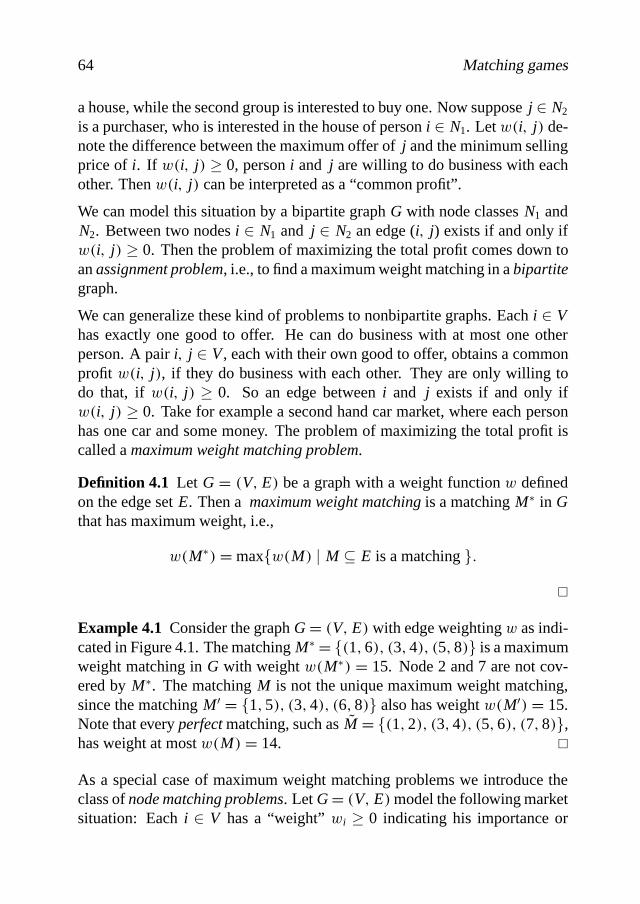
64 Matching games
a house, while the second group is interested to buy one. Now supposej ∈ N2
is a purchaser, who is interested in the house of personi ∈ N1. Letw.i; j/ de-note the difference between the maximum offer ofj and the minimum sellingprice of i. If w.i; j/ ≥ 0, personi and j are willing to do business with eachother. Thenw.i; j/ can be interpreted as a “common profit”.
We can model this situation by a bipartite graphG with node classesN1 andN2. Between two nodesi ∈ N1 and j ∈ N2 an edge (i; j) exists if and only ifw.i; j/ ≥ 0. Then the problem of maximizing the total profit comes down toanassignment problem, i.e., to find a maximum weight matching in abipartitegraph.
We can generalize these kind of problems to nonbipartite graphs. Eachi ∈ Vhas exactly one good to offer. He can do business with at most one otherperson. A pairi; j ∈ V, each with their own good to offer, obtains a commonprofit w.i; j/, if they do business with each other. They are only willing todo that, ifw.i; j/ ≥ 0. So an edge betweeni and j exists if and only ifw.i; j/ ≥ 0. Take for example a second hand car market, where each personhas one car and some money. The problem of maximizing the total profit iscalled amaximum weight matching problem.
Definition 4.1 Let G= .V; E/ be a graph with a weight functionw definedon the edge setE. Then a maximum weight matchingis a matchingM∗ in Gthat has maximum weight, i.e.,
w.M∗/ =max{w.M/ | M ⊆ E is a matching}:
�
Example 4.1 Consider the graphG= .V; E/ with edge weightingw as indi-cated in Figure 4.1. The matchingM∗ = {.1;6/; .3;4/; .5;8/} is a maximumweight matching inG with weightw.M∗/ = 15. Node 2 and 7 are not cov-ered byM∗. The matchingM is not the unique maximum weight matching,since the matchingM′ = {1;5/; .3;4/; .6;8/} also has weightw.M′/ = 15.Note that everyperfectmatching, such asM = {.1;2/; .3;4/; .5;6/; .7;8/},has weight at mostw.M/ = 14. �
As a special case of maximum weight matching problems we introduce theclass ofnode matching problems. Let G= .V; E/model the following marketsituation: Eachi ∈ V has a “weight”wi ≥ 0 indicating his importance or
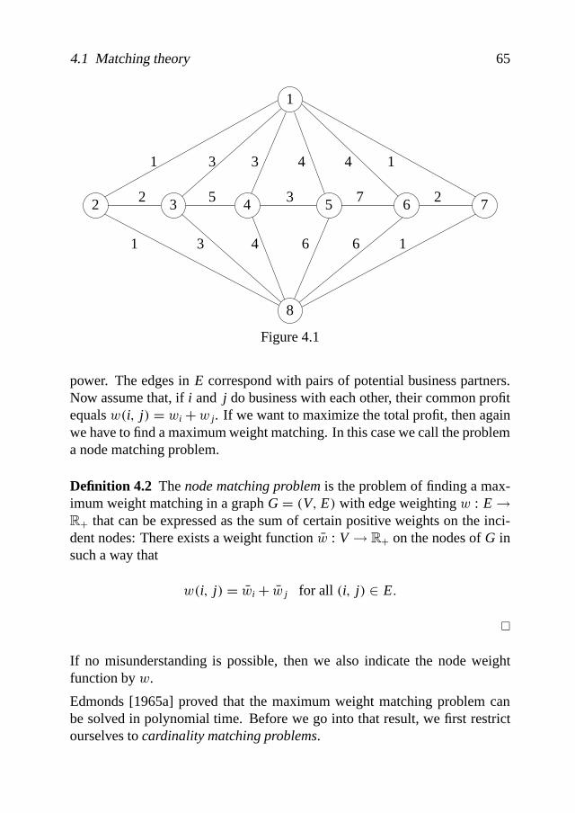
4.1 Matching theory 65
7 2
3 4 6 6 11
1
2
3 3 4 4 1
5 32
1
3 4 5 6 7
8
Figure 4.1
power. The edges inE correspond with pairs of potential business partners.Now assume that, ifi and j do business with each other, their common profitequalsw.i; j/ = wi +w j. If we want to maximize the total profit, then againwe have to find a maximum weight matching. In this case we call the problema node matching problem.
Definition 4.2 Thenode matching problemis the problem of finding a max-imum weight matching in a graphG= .V; E/ with edge weightingw : E→R+ that can be expressed as the sum of certain positive weights on the inci-dent nodes: There exists a weight functionw : V→ R+ on the nodes ofG insuch a way that
w.i; j/ = wi + w j for all .i; j/ ∈ E:
�
If no misunderstanding is possible, then we also indicate the node weightfunction byw.
Edmonds [1965a] proved that the maximum weight matching problem canbe solved in polynomial time. Before we go into that result, we first restrictourselves tocardinality matching problems.
66 Matching games
A maximum matchingin a graphG= .V; E/ is a matchingM∗ of maximumcardinality, i.e.,
|M∗| =max{|M| | M ⊆ E is a matching}:
The problem of finding a maximum matching in a graph is called thecardi-nality matching problem. Note that this problem can been seen as the simplestcase of a node matching problem by defining a node weightingw ≡ 1
2 on V.
A minimum node coveris a node coverV∗ ⊆ V of minimum cardinality, i.e.,
|V∗| = min{|V′| | V′ ⊆ V is a node cover}:
The following well-known min-max relation, valid for bipartite graphs, is dueto Konig [1931].
Theorem 4.1 The size of a maximum matching in a bipartite graph G=.V; E/ is equal to the size of a minimum node cover in G. �
Edmonds [1965b] constructed a polynomial time algorithm for solving thecardinality matching problem. The main idea is to find anaugmenting path.
Let M be a matching in a graphG= .V; E/. A pathP= v0v1 : : : vk in G is analternating path(relative toM) if for each i = 1; : : : ; k− 1 either.vi−1; vi/
or .vi; vi+1/ belongs toM. A path P= v0v1 : : : vk in G is called augmenting(relative toM), if P is alternating and both nodesv0 andvk are not covered byM. So the edges.v0; v1/; .v2; v3/; : : : ; .vk−1; vk/ do not belong toM, whilethe edges.v1; v2/; .v3; v4/; : : : ; .vk−2; vk−1/ belong toM. Note that in thiscase the length ofP is odd.
For two subsetsE1; E2 ⊆ E we let E14 E2 denote the setE1\E2 ∪ E2\E1.It is straightforward to see that, for a matchingM and alternating pathP;M4 P is again a matching inG. We say thatM4 P is the matching obtainedafter reversing M along P. If P is augmenting, then|M 4 P| = |M|+ 1.Furthermore, it is not difficult to prove the following lemma.
Lemma 4.1 Let G= .V; E/ be a graph and let M1;M2 be matchings in G.Then each component of the graph G′ = .V;M14 M2/ is either an alternat-ing path (possibly of length0) or an even cycle. �
To check whether a matchingM is a maximum matching or not, it is sufficientto know whether there exists an augmenting path.
4.1 Matching theory 67
Theorem 4.2 Let M be a matching in a graph G= .V; E/. Then either M isa maximum matching, or there exists an augmenting path relative to M.
Proof: If M is a maximum matching andP is an augmenting path, thenM4P would be a larger matching, a contradiction.
If M is not a maximum matching, then there exists a matching|M′| > |M|.At least one of the components inG′ = .V;M14 M2/ contains more edgesof M′ than ofM. By Lemma 4.1, such a component must be an augmentingpath. �
The running time of the cardinality matching algorithm of Edmonds [1965b]is bounded byO.|V|4/. Over the years this method has been sharpened (fora survey, see Lov´asz and Plummer [1986]). Eventually Micali and Vazirani[1980] showed that the running time can be reduced toO.|V| 12 |E|/.Theorem 4.3 Given a graph G= .V; E/, a maximum matching can be foundin time bounded byO.|V| 12 |E|/. �
For our main results, as stated in Section 4.3, we make use of theGallai-Edmonds decompositionof a graph. In order to describe this decompositionwe need the following basic concepts.
A (near-)perfect matchingis a matching that covers all nodes (except one). Agraph is factor-critical if removing any node results in a perfectly matchablegraph.
Let V′ ⊆ V. We letC = C.V′/ denote the set of even components ofG\V′andD = D.V′/ the set of odd components ofG\V′. The subsetV′ ⊆ V iscalled aTutte set, if each maximum matchingM of G decomposes as
M = MC ∪ MV′;D ∪ MD;
where MC is a perfect matching in⋃C, the union of all even components.
MD induces a near-perfect matching in all odd componentsD ∈ D andMV′;Dis a matching that matchesV′ (completely) into
⋃D, the union of odd com-
ponents. Note thatMV′;D has to match eachi ∈ V′ in a different componentD ∈ D.
Equivalently,V′ is a Tutte-set if and only if the sizem∗ of a maximum match-ing in G equals
m∗ =∑C∈C
|C|2+ |V′|+
∑D∈D
.|D| − 1/2
:

68 Matching games
Tutte sets can be found efficiently. More precisely, the following result, whichhas been proven by both Gallai [1963], Gallai [1964] and Edmonds [1965b],is true.
Theorem 4.4 (Gallai-Edmonds Decomposition).Given G= .V; E/, one canefficiently construct a unique Tutte set T⊆ V such that
(i) all odd components D∈ D are factor-critical
(ii) for each D∈ D there is some maximum matching that does not com-pletely cover D.
�
Let G= .V; E/ be a graph with node setV and edge setE. SupposeT ⊆ V isthe Tutte set satisfying condition (i) and (ii) of the theorem above. Clearly, anodev ∈ V is a node in
⋃D if and only if there exists a maximum matching
in G not coveringv.
Remark 4.1 The cardinality matching algorithm of Edmonds [1965b] can beused to construct the Tutte setT as described in Theorem 4.4. Given a graphG= .V; E/, we compute the sizem∗ of a maximum matching inG. We nextcompute for alli ∈ V the size of a maximum matching inG\i. If this size isequal tom∗, theni is a node in
⋃D. Otherwisei is not a node in
⋃D. Then
the subset ofV\V.⋃D/ that consists of all nodesv ∈ V adjacent to at least
one node in⋃D forms the required Tutte setT. �
Example 4.2 Let G = .V; E/ be the graph as shown in Figure 4.2. It isstraightforward to see that the setT = {v1; v2} is the unique Tutte set satisfy-ing conditions (i) and (ii) of Theorem 4.4. We haveD = D1∪ D2∪ D3∪ D4
andC = C1∪C2. �
We now return to the general maximum weight matching problem. LetG=.V; E/ be a complete graph with even node setV and edge weightingw. Aminimum weight perfect matchingis a perfect matchingM∗ in G that has
minimum weight, i.e.,
w.M∗/ = min{w.M/ | M ⊆ E is a perfect matching}:
Edmonds [1965a] obtained the following result.

4.1 Matching theory 69
1
4
2
2
21
3
1
C C
v
D
v
D
D
D
Figure 4.2. Gallai-Edmonds decomposition of a graph
Theorem 4.5 Let G= .V; E/ be a complete graph with even node set V andedge weightingw : E→ R. Then a minimum weight perfect matching in Gcan be found in polynomial time. �
This theorem implies that also the maximum weight matching problem canbe solved efficiently. This can be seen as follows. LetG= .V; E/ be a graphwith edge weightingw : E→ R. Since edges with negative weights will notoccur in any maximum weight matching, we may without loss of generalityassume thatw ≥ 0. If G is not already a complete graph, we add edges withzero weight. If|V| is odd, then we add a nodeu to V and edges fromu tothe nodes inV with zero weight. This way we have extendedG to a completegraph G. Finding a maximum weight matching inG is now equivalent tofinding a minimum weight perfect matching inG with edge weightingw givenby w.e/ = −w.e/ for all e∈ G.E/.
Corollary 4.1 Let G= .V; E/ be a graph with edge weightingw : E→ R.Then a maximum weight matching in G can be found in polynomial time.�

70 Matching games
A minimum weight maximum matchingin a graphG = .V; E/ with edgeweightingw : E→ R is a maximum matchingM∗ that has minimum weight,i.e.,
w.M∗/ = min{w.M/ | M ⊆ E is a maximum matching}:
Also the next result is a direct consequence of Theorem 4.5.
Corollary 4.2 Let G= .V; E/ be a graph with edge weightingw : E→ R.Then a minimum weight maximum matching in G can be found in polynomialtime.
Proof: If G is not already a complete graph, then we add edges with a suffi-cient large weight, sayw.E/+ 1. If |V| is odd, then we add a nodeu to Vand edges fromu to the nodes inV with weightw.E/+ 1. This way we haveextendedG to a complete graphG. Then computing a minimum weight max-imum matching inG is equivalent to computing a minimum weight perfectmatching inG. �
4.2 Matching games in general
4.2.1 Introduction
Consider again the example of an exchange market consisting of a group ofpersonsN as described in Section 4.1: Eachi ∈ N has exactly one good tooffer and can do business with at most one other person. A pairi; j ∈ N isonly willing to do business with each other, if they obtain a common profitw.i; j/ ≥ 0. So an edge betweeni and j only exists in casew.i; j/ ≥ 0.Obviously the total profit will be maximal, if all persons inN cooperate and amaximum weight matching can be constructed. The problem of dividing thetotal profit among the persons inN can be modeled as a matching game.
Definition 4.3 A matching game(N; v) is determined by a graphG= .N; E/with node setN and by a rational weight functionw ≥ 0 defined on the edgesetE. The valuev.S/ of a coalitionS⊆ N is the value of a maximum weightmatching in the subgraph induced byS. �
In this definition we assume thatw is a positive function, since edges witha negative weight will not occur in any maximum weight matching. It is

4.2 Matching games in general 71
straightforward to see that
v.S/+ v.T/ ≤ v.S∪ T/ for all S;T ⊆ N; S∩ T = ∅:
So a matching game is superadditive, andv.N/ is the maximum total profitthat players inN can obtain. Furthermore,v.i / = 0 for all individual playersi ∈ N.
The underlying discrete structure of a matching game (N; v) is a graphG andan edge weightingw. Let< w > again denote the maximum size of the edgeweights, i.e.,< w >= max{< w.i; j/ > | .i; j/ ∈ E}. Then we may define< N; v >= |N| < w >.
Example 4.3 Consider the graphG= .N; E/with edge weightingw as shownin Figure 4.3. The matching game (N; v) obtained from this graph is deter-mined byN = {1;2;3;4} andv : 2N→ R+ given by
31
5
2
31
21
34
Figure 4.3
v.1/ = 0 v.1;2/ = 2 v.1;2;3/ = 3 v.N/ = 7:v.2/ = 0 v.1;3/ = 3 v.1;2;4/ = 2v.3/ = 0 v.1;4/ = 1 v.1;3;4/ = 5v.4/ = 0 v.2;3/ = 3 v.2;3;4/ = 5
v.2;4/ = 1v.3;4/ = 5
�

72 Matching games
Given a graphG = .N; E/ and edge weightingw, a node matching gamearises if a positive weight functionw : N→ R+ on the nodes ofG exists insuch a way that
w.i; j/ = wi + w j for all .i; j/ ∈ E:
If w ≡ 1 (or equivalentlyw ≡ 12), then we call the corresponding node match-
ing game acardinality matching game.
A matching game associated with a bipartite graph is called anassignmentgame. Shapley and Shubik [1972] introduced this game and showed that thecore of an assignment game is always nonempty. Assignment games havebeen widely studied in the literature (see, e.g., Quint [1991], Granot and Gra-not [1992]). Solymosi and Raghavan [1994] present an efficient algorithm forcomputing the nucleolus of an assignment game.
With respect to a general matching game, Faigle, Kern, Fekete and Hochst¨attler[1998] present an efficient algorithm for computing the nucleon and point outthat the problem of computing the nucleolus remains unsolved. In the nextsection we summarize the results known for general matching games.
4.2.2 Solution concepts for matching games
The simplest matching game is a matching game (N; v) determined byG=K2, the complete graph on two nodes. The core of this game is equal to
core.N; v/ = {x∈ R2 | x1+ x2 = w.1;2/ andx≥ 0};
and the nucleolus of (N; v) is the allocation.12w.1;2/;
12w.1;2//.
During the rest of this chapter we will assume thatG 6= K2. In contrast toan assignment game, a general matching game can have an empty core. Thiscan already be the case for a matching game on three nodes (cf. Example 2.3,which can be interpreted as a matching game). Below we give some moreexamples of (cardinality) matching games with empty core. We have alsocomputed the nucleolus of these games.
Example 4.4 Let G = .N; E/ be the graph with edge weightingw ≡ 1 asshown in Figure 4.4.N is split into {t} ∪ N.D1/ ∪ N.D2/. Consider thestandard procedure for computing the nucleolus (see Section 2.3). The linear

4.2 Matching games in general 73
2
t
1D
D
Figure 4.4
program (P1) has already a unique optimal solution: the nucleolus�.N; v/given by
�i.N; v/ ={
47 if i = t37 if i ∈ N.D1/∪ N.D2/
andž1 = −37. �
Example 4.5 Let G = .N; E/ be the graph with edge weightingw ≡ 1 asshown in Figure 4.5. We haveN = N.D1/∪ N.D2/∪ N.D3/. Thenž1=−1andP1.−1/ contains all allocationsx∈ RN for which
xi = xj .i; j ∈ N.Dp/; p= 1; : : : ;3/xi + xj = 1
2 .i ∈ N.D1/; j ∈ N.D2//
xi = 12 .i ∈ N.D3//
x ≥ 0:
The nucleolus�.N; v/ is given by
�.N; v/ ≡ 14 on N.D1/∪ N.D2/
�.N; v/ ≡ 12 on N.D3/:
�
For E′ ⊆ E we let N.E′/ denote the set of nodes covered byE. If no mis-understanding is possible, we also use the following shorthand notation: If

74 Matching games
3
21D D
D
Figure 4.5
e= .i; j/ ∈ E, we write x.e/ = x.{i; j}/. More generally, ifM ⊆ E is amatching, we letx.M/ := x.N.M//. The following theorem gives an alter-native characterization of the core of a matching game. It turns out that onlythe core constraints for the one-and two-person coalitions are of importance.
Theorem 4.6 Let (N; v) be a matching game obtained from a graph G=.N; E/ with edge weightingw. Then core(N; v) equals the set of allocationsx∈ RN that are in the polyhedron Pc defined by the following constraints:
Pc x.N/ = v.N/x.e/ ≥ w.e/ for all e ∈ Exi ≥ 0 for all i ∈ N:
If x ∈ core(N; v), then
(i) xi = 0 for all i ∈ N not covered by a maximum weight matching.
(ii) x.e/ = w.e/ for all e ∈ E contained in a maximum weight matching.
Proof: The proof of the first part is straightforward, using the fact that theabove constraints implyx.S/ ≥ v.S/ for all S⊂ N.
Suppose core(N; v) is nonempty, and letx ∈ core(N; v). Let M be a max-imum weight matching inG. The core constraints implyx.N/ = v.N/ =w.M/; x≥ 0 andx.e/ ≥ w.e/ for all e∈ M. Then
w.M/ = x.N/ = x.N\N.M//+ x.M/ ≥ x.M/ ≥ w.M/
implies thatxi = 0 for all i =∈ N.M/ andx.e/ = w.e/ for all e∈ M. �
So, for matching games the number of inequalities defining the core have beenreduced to a polynomial number.

4.2 Matching games in general 75
Corollary 4.3 Checking whether the core of a matching game (N; v) is emptyor not can be done in polynomial time. �
By definition, the least core of a matching game (N; v) contains all optimalsolutions of the linear program
.LC/ max ž
s:t: x.S/ ≥ v.S/+ ž .S 6= ∅; N/x.N/ = v.N/:
Let ž∗ denote the optimal value of (LC). Also computing an element in theleast core of a matching game (N; v) can be done in polynomial time. Inorder to prove this we need the following lemmas. Recall that we assume thatG 6= K2, in which casež∗ = 1
2w.i; j/.
Lemma 4.2 Let (N; v) be a matching game. Thenž∗ = 0 if core(N; v) isnonempty, andž∗ < 0 if core(N; v) is empty.
Proof: Obviously ž∗ ≥ 0 if and only if core(N; v) is nonempty. Supposež∗ > 0 andx ∈ RN is an allocation in the least core of (N; v). Let M be amaximum weight matching. Sincež∗ > 0; x is also a core allocation. ByTheorem 4.6x.e/ = w.e/ for an edgee∈ M, which contradicts the least coreconstraintx.e/ ≥ w.e/+ ž > w.e/. �
Lemma 4.3 Let (N; v) be a matching game. Then leastcore(N; v) ⊆ RN+.
Proof: If core(N; v) is nonempty, the lemma follows trivially from Theorem4.6. Suppose core(N; v) is empty, and assume to the contrary that (x; ž1) is anoptimal solution of (LC), andxi < 0 for somei ∈ N. By Lemma 4.2ž1 < 0.
Claim: If S⊆ N satisfiesx.S/ ≥ v.S/+ ž1 with equality, theni ∈ S.
Proof: Assume to the contrary thati =∈ S.
case (i) S⊂ S∪ i ⊂ N.Thenx.S∪ i / < x.S/ = v.S/+ ž1 ≤ v.S∪ i /+ ž1 contradicts the feasibilityof x.
case (ii) S⊂ S∪ i = N.Thenx.N/ = x.S/+ xi = v.S/+ ž1+ xi < v.S/ ≤ v.N/ again contradictsthe feasibility ofx.
Hence the claim is true. But then we may slightly increasexi and decreasexon N\i uniformly by the same total amount, thereby obtaining a better solu-tion. This proves the lemma. �

76 Matching games
Due to Lemma 4.3, the linear program (LC) is equal to (P1), the first linearprogram that has to be solved in order to compute the nucleolus (see Section2.3). Lemma 4.3 also implies that the nucleolus is nonempty for all matchinggames. LetM denote the set of matchingsM ⊆ E. Then both linear programscan now be stated as
.P1/ max ž
s:t: x.M/ ≥ w.M/+ ž .M ∈M/
x.N/ = v.N/x ≥ 0:
Theorem 4.7 Computing an allocation in the least core of a matching game(N; v) can be done in polynomial time.
Proof: By Theorem 2.3 it suffices to show that for givenx∈RN andž ∈Rwecan efficiently check whetheremin.x/ ≥ ž or not. Since we can formulate thelinear program (LC) as the linear program (P1) described above, this comesdown to check whether
x.M/ ≥ w.M/+ ž .M ∈M/
holds. This can be done by solving a maximum weight matching problem onG= .N; E/ with respect to the edge weights
w.i; j/ := w.i; j/− xi − xj ..i; j/ ∈ E/:
Hence applying Corollary 4.1 finishes the proof. �
Faigle, Kern, Fekete and Hochst¨attler [1998] showed that the nucleon of amatching game can be computed in polynomial time. For a matching gamewith a nonempty core this also holds for the nucleolus.
Proposition 4.1 Let (N; v) be a matching game. If core(N; v) is nonempty,then the nucleolus of (N; v) can be computed in polynomial time.
Proof: We define
.P+1 / max ž
s:t: x.e/ ≥ w.e/+ ž .e∈ E/xi ≥ ž .i ∈ N/
x.N/ = v.N/

4.3 Node matching games 77
with optimum valuež+1 ∈ R. (In factž+1 = 0 holds, cf. Lemma 4.2). Next weidentify
E1 := {e∈ E | e∈ Fix P+1 .ž+1 /} andN1 := {i ∈ N | i ∈ Fix P+1 .ž
+1 /}
and then solve
.P+2 / max ž
s:t: x.e/ = w.e/+ ž+1 .e∈ E1/
xi = ž+1 .i ∈ N1/
x.e/ ≥ w.e/+ ž .e∈ E\E1/
xi ≥ ž .i ∈ N\N1/
x.N/ = v.N/
with optimum valuež+2 = ž2 etc. until we obtain a linear program (P+r ) thatdefines a unique solutionx∗ ∈ RN. Using the fact that the constraintsx≥ 0andx.e/ ≥ w.e/ for all e∈ E imply x.S/ ≥ v.S/ for all S⊂ N, it is clearthatx∗ is equal to the nucleolus of (N; v). �
The above approach fails in casež1 < 0. Whether there exists an efficientalgorithm for computing the nucleolus of a general matching game is notknown. In the next section we restrict ourselves to node matching games. Weshow that for this class of matching games the nucleolus can be computed inpolynomial time. This generalizes the result of Kern and Paulusma [2000],where cardinality matching games are considered. We first give a polyno-mial description of the least core. Next, we use this description to present anefficient algorithm for computing the nucleolus.
4.3 Node matching games
Recall that node matching games arise when the edge weightsw.e/ are thesum of certainpositiveweights on the incident nodes. In this section weconsider a node matching game (N; v) that is obtained from a graphG =.N; E/ with node weightingw : N→ R+. The edge weightingw is definedbyw.i; j/ = wi +w j for all .i; j/ ∈ E.
We use the following standard notation: ForS⊆ N we let E.S/ ⊆ E denotethe set of edges joining nodes ofS. Recall thatN.E′/ denotes the set of nodes
78 Matching games
covered by a subsetE′ ⊆ E. Furthermore, forS⊆ N we use the shorthandnotation
w.S/ =∑i∈S
wi :
Note thatw.S/ ≥ v.S/. Recall that we use the same notation for a matchingM ⊂M, i.e.,
w.M/ =∑e∈M
w.e/ =∑.i; j/∈M
.wi +w j /:
We assume thatT ⊆ N is the Tutte set satisfying the conditions (i) and (ii)in Theorem 4.4. The setM∗ denotes the set of maximum weight matchingsin G, andM∗ denotes the set of maximum matchings inG. EachM ∈M∗
matchesT completely inD. By condition (ii) of Theorem 4.4, givenD ∈ D,there is someM ∈ M∗ matchingT into D\{D}. We say thatM leaves Duncovered.
We will sometimes identify subsets ofN with the corresponding induced sub-graphs. For example, ifi ∈ N is a node, we do not hesitate to writei ∈ D toindicate thati is a node of the componentD ∈ D. If x ∈ RN is an allocation,we consequently write
x.D/ =∑i∈D
xi :
Each maximum weight matching can be extended to a maximum matching inthe following sense.
Lemma 4.4 Let M ∈ M∗ be a maximum weight matching. Then there existsa matching M∈M∗ in such a way that N.M/ ⊆ N.M/.
Proof: SupposeM ∈ M∗ is a maximum weight matching not already inM∗.By definition of the Tutte setT every maximum matchingM ∈ M∗ covers⋃C and matchesT completely into
⋃D. Now choose a maximum matching
M ∈ M∗ in such a way that all nodes in each componentD ∈ D that arecovered byM∗, also are covered byM. That this is possible can be seen asfollows. SupposeM does not cover a nodei ∈
⋃D that is covered byM.
Consider the maximum alternating pathP⊆ M ∪ M starting ini and endingin j. (Such a path exists according to Lemma 4.1.) SinceM ∈M∗; j is notcovered byM. ReversingM alongP results in a matchingM ∈M∗ covering

4.3 Node matching games 79
N.M/\ j ∪ i. For other nodes that are covered byM, but no byM, we do thesame. Hence we may assume thatM covers.N.M/∩
⋃C/∪ .N.M/∩ T/∪
.N.M/∩⋃D/ = N.M/. �
If M ∈ M∗ and M ∈ M∗ with N.M/ ⊆ N.M/, then obviouslyw.M/ =w.M/. SoM∗ ⊆M∗ holds if the node weightingw is strictly positive.
The following lemma gives a lower bound on the valuev.N\i / for all i ∈⋃D.
Lemma 4.5 For all i ∈⋃D, v.N\i / ≥ v.N/ − wi . If w > 0 on D then
v.N\i / > v.N/−wi holds.
Proof: SupposeD ∈ D andi ∈ D. If M∗ ∈ M∗ is a maximum weight match-ing not coveringi, thenv.N\i / = v.N/ ≥ v.N/−wi.
Otherwise assume thati is covered by a matchingM ∈ M∗. By Lemma4.4 we may assume thatM is a maximum matching. According to Theorem4.4 there exists a maximum matchingM′ ∈M∗ not coveringD. SinceD isfactor-critical, we may assume thatM′ does not coveri.
By Lemma 4.1 there exists a unique maximal alternating pathP⊆ M ∪ M′
starting ini and ending in a nodej. Since both matchingsM and M′ coverT ∪
⋃C; j must be a node in a componentD′ ∈ D (possibly equal toD).
ReversingM along P results in a matchingM ∈M∗ coveringN.M/\i ∪ j.Hencev.N\i /≥ w.M/=w.M/−wi +w j = v.N/−wi +w j, which provesthe lemma. �
The next result gives a sufficient condition for the core to be nonempty. If thenode weightingw : N→ R+ is strictly positive, then this is also a necessarycondition.
Theorem 4.8 If |D| = 1 for all D ∈ D, then core(N; v) is nonempty. If thenode weightingw : N→ R+ is strictly positive, then also the reverse state-ment is true.
Proof: Suppose|D|= 1 for all D ∈ D. Delete the componentsC ∈ C and alledges between nodes inT. In this way a graphG′ with node setN′ = T∪
⋃D
has been constructed. OnG′ we define the same node weightingw (restrictedto T ∪
⋃D). SinceG′ is bipartite, the corresponding node matching game
(N′; v′/ has a nonempty core (Shapley and Shubik [1972]).

80 Matching games
Choose an allocationx∈ core(N′; v′) in such a way thatxi ≥ wi for all i ∈ T.Such an allocation exists by the following reasoning. Add toG′ an extra nodes with weightws= 0 and connects to each node inT. This new graph is alsobipartite and the corresponding matching game (N′ ∪ s; v′′) has a nonemptycore. By Lemma 4.4 a maximum weight matching inG′ exists that matches allnodes inT. Then the value of a maximum weight matching has not increasedafter adding the extra nodes. Hence a core allocationx of the node matchinggame.N′ ∪ s; v′′/ (restricted toN′) lies in core.N′; v′/. By Theorem 4.6 wehavexs= 0. Thenxi = xi + xs≥ wi +ws= wi for all i ∈ T. Hencex′ ∈ RN
defined by
x′ ≡ wc on⋃C
x′ ≡ x on T ∪⋃D
is easily seen to be an element in core(N; v).
Supposew > 0 onD and D ∈ D with |D| ≥ 3. Let e= .i; j/ ∈ E.D/. ByLemma 4.5 we havev.N\i / > v.N/− wi andv.N\ j/ > v.N/− w j. So ifx∈ RN were in the core, then
x.N\i / ≥ v.N\i / > v.N/−wi and x.N\ j/ ≥ v.N\ j/ > v.N/−w j :
Together withx.N/= v.N/ these inequalities implyxi+ xj <wi+w j, a con-tradiction with the core constraintx.e/= xi+ xj ≥wi+w j. Hence core(N; v)must be empty. �
The following result shows that, according to a core allocationx ∈ RN, theamount that is allocated to a nodei ∈ D does not exceed the weightwi. Thisimplies thatxi = 0 for a nodei ∈
⋃D with weightwi = 0.
Proposition 4.2 If core(N; v) is nonempty, then for all x∈ core(N; v)
xi ≤ wi for all i ∈⋃D:
If D ∈ D has size|D| > 1, then xi = wi holds for all i∈ D.
Proof: SupposeD ∈ D and i ∈ D. Let x ∈ RN be a core allocation. ByLemma 4.5,v.N\i / ≥ v.N/ − wi. Then xi = x.N/ − x.N\i / ≤ v.N/ −v.N\i / ≤ wi.
If |D| > 1 then there is a nodej ∈ D such that.i; j/ is an edge inE. Sincex ∈ core(N; v), xi + xj ≥ wi +w j. Since we have just deduced thatxi ≤ wi
andxj ≤ w j, this implies thatxi = wi (andxj = w j). �

4.3 Node matching games 81
4.3.1 The least core of node matching games
Recall that, due to Lemma 4.3, the linear program defining the least core canbe stated as the linear program
.P1/ max ž
s:t: x.M/ ≥ w.M/+ ž .M ∈M/
x.N/ = v.N/x ≥ 0
with optimal valuež1 ≤ 0. In the following we assume that core(N; v) isempty. Equivalently, by Lemma 4.2ž1 < 0. Furthermore, by Theorem 4.8there exists at least one componentD ∈ D with size|D| > 1.
Example 4.6 Consider the node matching game (N; v) obtained from thegraphG= .N; E/ with node weightingw as indicated in Figure 4.6.
3
1
2
2
5
3
15
1
6 7
43
2
Figure 4.6
Clearly, the setT = {5} is the Tutte set satisfying conditions (i) and (ii) ofTheorem 4.4. The graphG\T has two odd componentsD1 with node set{1;2;3} and D2 with node set{4}, and one even componentC1 with nodeset{6;7}. By Theorem 4.8 core(N; v) is empty.

82 Matching games
The value of a maximum weight matching inG is equal tov.N/ = 16. Let(x; ž) be a feasible solution for.P1/. Thenx1+ x2≥ 6+ ž; x.N\1/ ≥ 12+ žandx.N\2/ ≥ 16+ ž. Together withx.N/ = 16 we obtain the upper boundž ≤ −2
3.
It is easy to check thatx= .423;
23;1
23;0;4;2;3/ is an allocation inP1.−2
3/.Hencež1 = −2
3. In fact, the allocations in leastcore(N; v/ = P1.−23 / turn out
to be exactly the allocations in the polyhedron determined by the constraints
x1 = 423
x2 = 23
x3 = 123
x3+ x5 ≥ 3x4+ x5 = 4x5+ x6 ≥ 3x6+ x7 = 5x.N/ = 16x ≥ 0:
�
By Theorem 4.7 we can efficiently compute an allocation in the least core of(N; v). Here we aim for more, namely a concise description ofP1.ž1/.
Note that in Example 4.6xi −wi = xj −w j ≤ 0 for all nodesi; j in the samecomponentD ∈ D. Also x.e/ ≥ w.e/ for all edges inE with at least oneend point not in
⋃D. Furthermore, large matchings such as the matching
M = {.1;2/; .4;5/; .6;7/} and matchings completely contained in⋃D turn
out to become tight, i.e., the corresponding constraints in (P1) become tight.Also for Example 4.4 and Example 4.5 this is true. Generally speaking, thisholds for any node matching game, i.e., we will prove that the least core of(N; v) can be described as the solution set of the following linear program.
max ž
s:t: xi −wi = xj −w j .i; j ∈ D; D ∈ D/xi ≤ wi .i ∈
⋃D/
x.e/ ≥ w.e/ .e∈ E\E.⋃D//
x.N/ = v.N/x ≥ 0
ž =∑D∈D
|D| − 1|D| .x.D/−w.D//:

4.3 Node matching games 83
In this description the exponentially many constraints defining the least corehave been replaced by a polynomially number.
If core(N; v) would be nonempty, this is straightforward to see: By Theorem4.6 core(N; v) is equal to the polyhedronPc. By Proposition 4.2 we may addthe constraintsx ≤ w on
⋃D, andxi = wi for all i ∈ D and D ∈ D with
|D| > 1. So, if core(N; v) would be nonempty, then the optimal solutions ofthe linear program as defined above describe the (least) core of (N; v).
However, we have assumed that core(N; v) is empty, and in the rest of thissection we show that also in this case the linear program.P1/ can be replacedby the linear program as described above. As a first step, we introduce arelaxation (P1) of (P1) below, which is easier to analyze and, as we shallsee, defines the same optimum value. To motivate this approach, note that,as shown in Example 4.6, rather large matchings and matchings completelycontained in
⋃D are expected to become tight when solving (P1) instead of
small ones (single nodes and edges) as in the case of a nonempty core.
LetMD denote the set of matchingsM ⊆ E.⋃D/ that are completely con-
tained in the union of the odd components. We shall study the followingrelaxation of (P1):
. P1/ max ž
s:t: x.M/ ≥ w.M/+ ž .M ∈M∗ ∪MD/x.N/ = v.N/
x ≥ 0
with optimal valuež1 ∈ R. Obviously ž1 ≤ 0. Below we will show thatž1 < 0. Note that we do not explicitly consider maximum weight matchingsin the description of (P1). However, by Lemma 4.4 we know that, in casethese matchings do not already belong to the setM∗ of maximum matchings,there exists a corresponding matchingM ∈M∗.
To investigate the structure of optimal solutions of (P1), we first introducesome notation. As before,P1.ž/ denotes the set ofx ∈ RN such that (x; ž) isfeasible for (P1). If x∈ P1.ž1/ is an optimal solution, we say thatM ∈M∗ ∪MD is x-tight, if x.M/ = w.M/+ ž1. Given a feasible solutionx ∈ P1.ž/
andD ∈ D, let
xD := x.D/|D|

84 Matching games
denote the average value ofx on D. In the same way we define the averageweight on a componentD ∈ D :
wD := w.D/|D| :
Define x ∈ RN by averaging x with respect to the node weightsw on eachcomponentD ∈ D, i.e.,
xi := xD−wD +wi .i ∈ D; D ∈ D/
and leavingx unchanged onT ∪⋃C. Note thatxi.D/ = x.D/, and
xi −wi = x j −w j for all i; j ∈ D:
First we show thatx ∈ P1.ž1/, if x ∈ P1.ž1/ is an optimal solution. In orderto this we need the following series of lemmas.
Lemma 4.6 Let x∈ P1.ž/ for somež < 0. If no x-tight matchings inMDexist, thenž is not optimal.
Proof: Supposex.M/ > w.M/+ ž for all matchingsM ∈MD. If no x-tightmatchings inM∗ exist either then, obviously,ž is not optimal. If M ∈ M∗
covers all nodesi ∈⋃D with xi > 0, then
x.M/ = x.N/ = v.N/ > v.N/+ ž;
which means thatM is notx-tight. Hence eachx-tight matching inM∗ doesnot cover all nodesi ∈
⋃D with xi > 0. Then we may slightly and uniformly
decreasex on the set{i ∈⋃D | xi > 0} and increase it by the same total
amount onT ∪⋃C. The resultingx has no tight matchings inM∗ ∪MD,
which implies thatž is not optimal. �
Lemma 4.7 If x ∈ P1.ž/ thenx.M/ ≥ w.M/+ ž for all M ∈M∗ ∪MD.
Proof: Let x ∈ P1.ž/. It suffices to show that the constraints above are stillsatisfied after averagingx with respect to the node weightingw on some com-ponentD ∈ D. Thus letD ∈ D and letx∈ RN be obtained by averagingx onD, i.e.,
xi = xD −wD +wi .i ∈ D/:

4.3 Node matching games 85
SupposeM ∈M∗. Then eitherM coversD or M ∩ D= D\i for somei ∈ D.In the first casex.M/ = x.M/ and the claim follows. In the second case wemay assume without loss of generality thati ∈ D maximizesxi − wi overD, otherwise we replaceM inside D by some other near-perfect matchingwithout changingx.M/−w.M/. (Recall thatD is factor-critical.) But thenxi − wi ≥ xD − wD = xi − wi and consequentlyx.M/− w.M/ ≥ x.M/ −w.M/, so the claim follows asx∈ P1.ž/.
Next considerM ∈MD and assumeM minimizesx.M/−w.M/ overMD.If xD −wD > 0 on D, thenM ∩ D = ∅. Hencex.M/ = x.M/ and the claimfollows. If xD − wD ≤ 0 on D, then M ∩ D is without loss of generality anear-perfect matching inD and we argue as we did forM ∈M∗. �
It is immediately clear thatx.N/ = x.N/. We still have to show thatx ≥ 0for an allocationx∈ P1.ž1/.
Lemma 4.8 If x ∈ P1.ž1/ thenx∈ P1.ž1/.
Proof: Let x ∈ P1.ž1/. Besidesx.N/ = v.N/ we have already shown, inLemma 4.7, thatx.M/ ≥ w.M/+ ž1 for all M ∈ M∗ ∪MD. Let wD
min de-note the minimum weight in a componentD ∈ D, i.e,wD
min = min{wi | i ∈D} .D ∈ D/. We will prove that for allD ∈ D
xD ≥ wD −wDmin:
Thenx≥ 0, and we are finished. Now supposeD′ ∈D andxD′ < wD′ −wD′min,
or equivalently, ∑i∈D′
xi <∑i∈D′
.wi −wD′min/:
Note that|D′| > 1. Let j ∈ D′ be a node withw j = wD′min. It is straightforward
to see that we can obtain an allocationx∈ RN such that
xi ≤ wi −w j .i ∈ D′/x.D′/ = x.D′/xi = xi .i ∈ N\D′/x ≥ 0:
We have chosenx in such a way thatxj = 0 and xi − wi ≤ x j − w j for alli ∈ D′\ j.

86 Matching games
• Below we show thatx is an allocation inP1.ž1/. Besidesx≥ 0, obviouslyx.N/ = v.N/. So we are left to check whetherx.M/ ≥ w.M/+ ž1 for allM ∈M∗ ∪MD.
SupposeM ∈M∗. Then eitherM coversD′ or M ∩ D′ = D′\i for somei ∈D′. In the first casex.M/ = x.M/ ≥ w.M/+ ž1. In the second case we de-duce thatx.D′\i /−w.D′\i / ≥ x.D′\ j/−w.D′\ j/ ≥ x.D′\ j/−w.D′\ j/,sincexi −w j ≤ xj −w j andxj = 0. BecauseD is factor-critical, we can re-place the edges inM coveringD′\i by 1
2.|D| − 1/ edges coveringD′\ j. Thisresults in a matchingM′ such that
x.M/−w.M/ ≥ x.M′/−w.M′/ ≥ ž1:
SupposeM ∈MD and assume thatM minimizesx.M/−w.M/ overMD.Sincexi ≤ wi −w j ≤ wi; M ∩ D′ is without loss of generality a near-perfectmatching inD′ and we argue as we did forM ∈M∗.
• Since x.D′/ = x.D′/ <∑
i∈D′.wi − w j /, there exists a nodek ∈ D′ forwhich xk < wk−w j, and consequently,xk−wk < x j −w j.
Claim: The nodek ∈ D′ is covered by everyx-tight matchingM ∈ M∗ ∪MD.
Proof: SupposeM ∈M∗ is x-tight. If M coversD′ then the claim follows.Otherwise|M ∩ D′| = |D′| − 1. SupposeM ∩ D′ = D′\{k}. Since xk −wk < x j −w j, we havex.D′\k/−w.D′\k/ > x.D′\ j/−w.D′\ j/. Then amatchingM′ ∈ M∗ would exist withN.M′/ = N.M/\ j ∪ k and x.M′/ <w.M′/+ ž1, contradicting the feasibility ofx.
SupposeM ∈ MD is x-tight. If |M ∩ D′| = |D′| − 1 then, from the above,M must coverk. Otherwise|M ∩ D′| < |D′| − 1. SupposeM does not coverk. Sincexi ≤ wi on D′, we can extendM to a tight matchingM′ inMD thatcoversD′\k, a contradiction.
• We now show that we can increasež1 by modifying x a little, which wouldcontradict the optimality ofž1. We first deduce thatž1≤ xk+ xi −wi −wk <
0, wherei ∈ N is chosen in such a way thati ∈ D′ and.i; k/ ∈ E.
Supposex.T ∪⋃C/ > 0. Then decreasex onT ∪
⋃C and increasexk by the
same amount in such a way that the resultingx′ is still in P1.ž1/. Clearly, x′
has no tight matchings inMD. By Lemma 4.6ž1 is not optimal, a contradic-tion.

4.3 Node matching games 87
Supposex.T ∪⋃C/ = 0. Thenx.
⋃D/ = x.N/ − x.T ∪
⋃C/ = x.N/ =
v.N/ ≥ v.⋃D/=∑D∈D.w.D/−wD
min/. Sincex.D′/ < w.D′/− |D′|wD′min,
there exists a componentD ∈ D with x.D/ > w.D/− |D|wDmin. By Lemma
4.7, we may assume that
xi = xD −wD +wi > 0 on D:
Then decreasex on D and increasexk by the same sufficient small amount.Again the resulting allocation has no tight matchings inMD, and ž1 wouldnot be optimal.
So we have showed that for allD ∈ D xD ≥ wD −wDmin, implying thatx≥ 0.
�
Lemma 4.9 ž1 < 0.
Proof: Supposex ∈ P1.ž1/. By Lemma 4.8 we may assume thatx = x.If xD < wD on someD ∈ D, then consider an edgee ∈ E.D/. We havež1 ≤ x.e/−w.e/ = 2.xD −wD/ < 0.
SupposexD ≥ wD for all D ∈ D. Let M be a maximum weight matching inM∗. If M covers alli ∈
⋃D with wi > 0, thenx′ given byx′i = wi is easily
seen to be a core allocation. This contradicts our assumption that core(N; v)is empty. Hence there exists a nodei in someD ∈ D with wi > 0 that isnot covered byM. Then xi = xD − wD + wi ≥ wi > 0, and consequently,x.M/ < x.M ∪ i / ≤ x.N/ = v.N/. Together withx.M/ ≥ v.N/+ ž1, thisimplies ž1 < 0. �
Summarizing we conclude thatž1 < 0. If x∈ P1.ž1/ is an optimal allocation,so is x. Furthermore, some matchings inM∗ ∪MD must bex-tight. Thesecan in principle be found by minimizingx.M/ − w.M/ overM∗ ∪MD.Minimizing x.M/−w.M/ overM∗ amounts to solving a minimum weightmaximum matching problem (cf. Corollary 4.2). Minimizingx.M/−w.M/overMD is even trivial: We simply choose a near-perfect matching in eachcomponentD ∈ D with xD < wD (plus an arbitrary matching in all compo-nents on whichxD = wD). So computing anx-tight M ∈M∗ ∪MD for givenx∈ P1.ž1/ is easy.
We aim at a more structural characterization ofx-tight matchings for givenx∈ P1.ž1/. LetDmax=Dmax.x/ ⊆D be the set of odd components on whichxD −wD is maximum (among allD ∈ D).

88 Matching games
Lemma 4.10 No x-tight M∈M∗ covers all D∈ Dmax. If x-tight matchingsin M∗ exist at all, then for each D∈ Dmax there is somex-tight M ∈ M∗
leaving D uncovered.
Proof: SupposeM ∈ M∗ is x-tight and coversD ∈ Dmax. Let M ∈ M∗ beany matching not coveringD. (Recall Theorem 4.4). LetP⊆ M ∪ M be theunique maximal alternating path starting inD (in a nodei uncovered byM)and ending in, say,D (in a nodej uncovered byM). ReversingM along Presults in a matchingM ∈M∗ coveringN.M/\i ∪ j ∈ D. SinceD ∈ Dmax,we havexi −wi = xD−wD ≥ xD −wD = x j −w j, hence
x.M/−w.M/ ≤ x.M/−w.M/:
Thus M must bex-tight again, proving the second claim. The first claimfollows by observing that ifM would cover allD ∈ Dmax, thenD =∈ Dmax (asit is uncovered byM). But thenxD −wD > xD −wD and x.M/−w.M/ <x.M/−w.M/ = ž1, contradictingx∈ P1.ž1/. �
LetM∗D denote the set of all maximum matchings inMD.
Lemma 4.11 Let x∈ P1.ž1/. Then
(i) x = x
(ii) x ≤ w on⋃D
(iii) Each M ∈M∗D is x-tight.
Proof: Let x ∈ P1.ž1/. We first prove (ii) and (iii) forx and then show thatx= x.
(ii) x≤ w on⋃D, or equivalently,xD ≤ wD for all D ∈ D:
Suppose to the contrary thatxD >wD ≥ 0 for some odd componentD ∈Dmax.Thenxi > wi ≥ 0 for all i ∈
⋃Dmax.
We first consider the caseT ∪⋃C = ∅. If Dmax= D, we hadx > wD for
all D ∈ D and hencex.N/ > v.N/, a contradiction. HenceDmax⊂ D. ByLemma 4.10 we may decreasex slightly and uniformly on
⋃Dmax and in-
creasex on⋃D\
⋃Dmax resulting in somex ∈ P1.ž1/ for which no M ∈
M∗ ∪MD is tight. This contradicts the optimality ofž1.

4.3 Node matching games 89
Now supposeT ∪⋃C 6= ∅. If Dmax= D, we hadxD > wD for all D ∈ D
and hence noM ∈MD werex-tight. By Lemma 4.6,ž1 < 0 is not optimal, acontradiction.
If Dmax⊂D, we proceed as follows. ChoseŽ > 0 sufficiently small and letxŽ
arise fromx by
� decreasingxi byŽ
|D| (i ∈ D; D ∈ Dmax)
� increasingx on T by Ž′ in total, where.|Dmax| − 1/Ž < Ž′ < |Dmax|Ž
� increasingx uniformly on⋃D\
⋃Dmax by |Dmax|Ž− Ž′ in total.
For sufficiently smallŽ > 0 the resultingxŽ has xŽ.M/ > x.M/ for eachx-tight M ∈MD (since none of these meetsDmax) and xŽ.M/ > x.M/ for allx-tight M ∈ M∗ by Lemma 4.10. Hence, againxŽ ∈ P1.ž1/ has no tightmatchings, contradicting the optimality ofž1.
(iii) Each M ∈M∗D is x-tight: First note that for anyM1;M2 ∈M∗
D,
x.M1/−w.M1/ = x.M2/−w.M2/ =∑D∈D
.|D| − 1/.xD −wD/:
SincexD ≤ wD for all D ∈ D, eachM ∈M∗D minimizesx.M/−w.M/ over
MD. Then the claim follows from Lemma 4.6.
(i) x= x:For eachD ∈ D we chose a nodei ∈ D with xi −wi =max{xj −w j | j ∈ D}and a near-perfect matching coveringD\i. Let M ∈ M∗
D be the union ofall these near-perfect matchings. By construction we havex.M/−w.M/ ≤x.M/− w.M/ with equality if and only ifx ≡ x on
⋃D. But sinceM is
x-tight,
x.M/−w.M/ < x.M/−w.M/ = ž1
would contradictx∈ P1.ž1/. �
Lemma 4.12 Let x= x∈ P1.ž1/. If x.T ∪⋃C/ = 0, then every M∈M∗ is
x-tight.

90 Matching games
Proof: If T∪⋃C is empty, thenM∗ =M∗
D and the claim follows by Lemma4.11(iii). SupposeT ∪
⋃C is nonempty andx.T ∪
⋃C/ = 0. Recall that any
M ∈M∗ decomposes as
M = MC ∪ MT;D ∪ MD
with MC a perfect matching of⋃C, MT;D matchingT completely into
⋃D
andMD ∈M∗D. SinceMD is x-tight (cf. Lemma 4.11(iii)), we havex.MD/=
w.MD/+ ž1. Together withx.M/ ≥ w.M/+ ž1, this implies
x.MC ∪ MT;D/ ≥ w.MC /+w.MT;D/:
Let B⊂⋃D be the set of nodes that is joined to the nodes inT by MT;D. Then
w.MC /+w.MT;D/ = w.T ∪⋃C/+w.B/. By Lemma 4.11(ii),xi ≤ wi for
all i ∈ B. Since we assumed thatx.T ∪⋃C/ = 0, we have
w.B/+w.T ∪⋃C/ ≤ x.B/ ≤ w.B/:
Thenw ≡ 0 onT ∪⋃C andxi = wi on B. Hence we deduce that
x.M/ = x.MC /+ x.T/+ x.B/+ x.MD/= w.B/+w.MD/+ ž1
= w.M/+ ž1:
�
Lemma 4.13 Let x= x∈ P1.ž1/. Then there is some x-tight M∈M∗. More-over, if D∈ Dmax or |D|> 1 then there is some x-tight M∈M∗ not coveringD.
Proof: If x.T ∪⋃C/ = 0 then, according to Lemma 4.12, everyM ∈M∗ is
x-tight. Since for eachD ∈ D there is some matchingM ∈M∗ not coveringD, we have finished this case.
Assume thatT ∪⋃C 6= ∅ andx.T ∪
⋃C/ > 0. Supposex.M/ > w.M/+ ž1
for all M ∈ M∗. Then we could do as follows: Decrease (somehow)x onT ∪
⋃C and increasex uniformly on
⋃D by the same total (sufficiently
small) amount. The resultingx were still in P1.ž1/ and would contradictLemma 4.11(iii).
By Lemma 4.10 this implies that eachD ∈ Dmax is left uncovered by somex-tight M ∈M∗. We are left to prove a corresponding result forD ∈ D with

4.3 Node matching games 91
|D|> 1. Assume thatD ∈D\Dmax and|D|> 1. Thenx<w on D by Lemma4.11(ii), so everyx-tight M ∈ M∗
D contains a near-perfect matching ofD.Now supposeD is covered by everyx-tight M ∈M∗. Sincex.T ∪
⋃C/ > 0,
we may decreasex slightly on T ∪ C and increasex uniformly on D by thesame (sufficiently small) total amount. The resulting¯x would again be inP1.ž1/ and contradict Lemma 4.11(iii). This finishes the proof. �
We call an allocationx= x∈ P1.ž1/ flexibleif the conclusion of Lemma 4.13holds with respect to allD ∈ D, i.e., if eachD ∈ D is left uncovered by somex-tight M ∈M∗.
Lemma 4.14 Flexible allocations exist.
Proof: Let x = x ∈ P1.ž1/. Supposex is not already flexible. Then thereexists a componentD = {i} ∈ D of size 1 such that everyx-tight M ∈M∗
coversi. Maximum matchings not coveringi are not tight. In particular, thisimplies thatT 6= ∅ and, by Lemma 4.12,x.T ∪
⋃C/ > 0.
We may thus increasexi and decreasex onT∪⋃C by the same total amountŽ
until x becomes “flexible” with respect toD= {i}. By Lemma 4.12 we knowthat this will happen beforeŽ exceeds the valuex.T ∪
⋃C/. In other words,
we chooseŽ > 0 maximal such that the modificationxŽ is still in P1.ž1/. ThenxŽ.M/= w.M/+ ž1 holds for a matchingM ∈M∗ that does not coveri (andis not x-tight). Because all matchings inM∗ that were alreadyx-tight (andcoveri) remain tight, the claim follows by induction. �
We are now ready to determine the structure ofx-tight matchings inM∗ forflexible x = x ∈ P1.ž1/. Supposex ∈ P.ž1/ is a given flexible allocation.Suppose thatÞ0 < : : : < Þp .p≥ 0/ are the different valuesx−w takes on⋃D and let
D = D0∪ : : : ∪Dp
be the corresponding partition ofD. Hencex− w ≡ Þi on⋃Di andDp =
Dmax.
Proposition 4.3 There exists a partition T= T0 ∪ : : : ∪ Tp (with some of theTi possibly empty) such that M∈M∗ is x-tight if and only if M matches eachTi intoDi .
Proof: If T = ∅, the claim is true in the sense that nothing is matched intoDand eachM ∈M∗ is x-tight. (By Lemma 4.13, somex-tight M ∈M∗ existsand sinceT = ∅, all M ∈M∗ have the samex-value.)

92 Matching games
In general, recall thatx-tight matchings inM∗ are exactly those that minimizex.M/−w.M/ overM∗. For givenx, the valuex.M/−w.M/ only dependson how many nodes ofT are matched into eachDi. (This readily follows fromthe decompositionM = MC ∪ MT;D ∪ MD.) In other words,x.M/− w.M/only depends on the total.x− w/-weight of nodes in
⋃D that are matched
with T. The claim therefore follows from Lemma 4.15 below. �
Lemma 4.15 Consider a bipartite graph G with node classes A and B. Sup-pose B= B0 ∪ : : : ∪ Bp is a partition of B and edges incident with Bi haveweightÞi (Þ0 < : : : < Þp/. Assume that the setM∗ of matchings that com-pletely match A into B is nonempty and letM∗
min be the set of M∈M∗ withminimum weight. Suppose finally, thatM∗
min is “flexible” in the sense thateach b∈ B is left uncovered by some M∈ M∗
min. Then there is a partitionA= A0∪ : : :∪ Ap of A such that M∈M∗
min if and only if M matches Ai intoBi (i = 0; : : : ; p).
Proof: LetM∗0 denote the set of maximum matchings in the subgraphG0
induced byA∪ B0. EachM ∈M∗min induces a maximum matchingM0 ⊆ M
inM∗0. This can be seen as follows: SupposeM does not induce a matching
M0 ∈M∗0. Let M′0 be a maximum matching inM∗
0. For all nodesb∈ B0 thatare covered byM′0 but not byM we do as follows. LetP⊆ M ∪ M′0 be theunique maximal alternating path starting in nodeb∈ B0 uncovered byM andending in a nodea uncovered byM′0. ReverseM along P. Then in the endthis results in a matchingM′ with w.M′/ < w.M/, a contradiction. Hencewe must have
.∗/ Eachb ∈ B0 is left uncovered by someM0 ∈M∗0:
Supposem∗0 is the maximum size of a matching inG0. As G0 is bipartite,Theorem 4.1 ensures the existence of a (minimum) node coverA∗0 ∪ B∗0(A∗0⊆ A; B∗0 ⊆ B) of sizem∗0. Since|A∗0∪ B∗0|= |M| for a matchingM ∈M∗
0,eachM ∈M∗
0 is incident with all nodes inA∗0 ∪ B∗0. Hence, by (*) we con-clude thatB∗0 = ∅. In other words, eachM ∈M∗
min matchesA∗0 into B0. NowletM∗
1 denote the set of maximum matchings in the subgraphG1 induced byA\A∗0∪ B1, and continue in the same way. So the claim follows by induction.
�

4.3 Node matching games 93
We are now prepared to present our main result, a simple alternative descrip-tion of the least core. Consider the LP
.ˆP1/ max ž
s:t: x = xxi ≤ wi .i ∈
⋃D/
x.e/ ≥ w.e/ .e∈ E\E.⋃D//
x.N/ = v.N/x.M/ ≥ w.M/+ ž .M ∈M∗
D/x ≥ 0:
Note thatx≡ x is just a shorthand notation for a number of linear equalitiesof the typexi − wi = xj − w j. Furthermore, note that forx ≡ x the valuex.M/−w.M/ is independent of the particular choice ofM ∈M∗
D. Hence theexponentially many constraints forM ∈M∗
D reduce to one single inequality.
Again, we let ˆP1.ž/ := {x | .x; ž/is feasible for. ˆP1/} and denote the optimum
value of ( ˆP1) by ˆž1.
Theorem 4.9 We havež1= ž1= ˆž1 and leastcore.N; v/= P1.ž1/= ˆP1. ˆž1/.
Proof:• We havež1 ≤ ž1 by definition.
• ž1 ≤ ˆž1: Let x∈ P1.ž1/ be flexible with corresponding partitionsD =D0∪ : : : ∪Dp andT = T0∪ : : : ∪ Tp. Define ˆx∈ RN by
ˆxi = wi if i ∈
⋃C
xi if i ∈⋃D
wi − Þ j if i ∈ Tj .0≤ j ≤ p/:
We show thatˆx ∈ ˆP1.ž1/ (proving that ˆž1 ≥ ž1). The only non-trivial con-straints to check arex.N/ = v.N/ and ˆx.e/ ≥ w.e/ for e∈ E\E.
⋃D/. All
other constraints directly follow from Lemma 4.11.
Let M ∈M∗ be x-tight and decompose it as
M = MC ∪ MT;D ∪ MD
as usual. SinceMD ∈M∗D is alsox-tight by Lemma 4.11, we conclude that
x.MC ∪ MT;D/ = w.MC / + w.MT;D/ = ˆx.MC ∪ MT;D/ by definition of ˆx.Hence ˆx.N/ = x.N/ = v.N/.

94 Matching games
Secondly, let us considere∈ E\E.⋃D/. If e∈ E.T ∪
⋃C/ then ˆx.e/ ≥
w.e/ by definition of ˆx. (Recall thatÞ j = xi −wi ≤ 0 for all i ∈⋃D j.) Thus
we are left with edges betweenT and⋃D. Supposex.e/ < w.e/ for such
an edge joining, say,D ∈ Di with k ∈ Tj. Then ˆx.e/ < w.e/ impliesÞi < Þ j.Sincex is flexible, there exists anx-tight matchingM ∈M∗ not coveringD.SinceD is factor-critical (andx−w is constant onD), we may assume thatMdoes not match the end point ofe in D. SinceM is x-tight, k ∈ Tj is matchedinto D j by some edgef ∈ M (cf. Proposition 4.3). But thenM′ = M\ f ∪ ehas x.M′/− w.M′/ = x.M/ − w.M/ + Þi − Þ j < x.M/ − w.M/ = ž1, acontradiction.
• ˆž1 ≤ ž1: We show that in generalP1.ž/ ⊆ P1.ž/. Supposex ∈ ˆP1.ž/.Thenx.M/ ≥ w.M/+ ž for all M ∈ M∗
D. Sincex ≤ w on⋃D, this also
impliesx.M/ ≥ w.M/+ ž for all M ∈MD. (Use an augmenting path argu-ment.) Sincex.e/ ≥ w.e/ for all e∈ E\E.
⋃D/, we further conclude that
x.M/ ≥ w.M/+ ž for all M ∈M.
• Finally, we verify thatP1.ž1/ = ˆP1. ˆž1/. We have just proved that “⊇”holds. Conversely letx∈ P1.ž1/. Thenx∈ P1.ž1/ and by Lemma 4.11x satis-
fies all constraints ofP1. ˆž1/ except possiblyx.e/≥w.e/ for e∈ E\E.⋃D/.
Thus lete∈ E\E.⋃D/. Pick M ∈M∗
D not covering the end point ofe in⋃D, so thatM ∪ e is a matching again. Then, sincex ∈ P1.ž1/, we have
x.M ∪ e/ ≥ w.M/ + w.e/ + ž1, and sinceM ∈ M∗D is x-tight, we have
x.M/ = w.M/+ ž1. Sincež1 = ž1, the claim follows. �
As mentioned before, the least core of a node matching game can also be
described by the polyhedronP1. ˆž1/ = ˆP1.0/ if the core is nonempty.
For general matching games it is not possible to characterize the least core by
a polyhedron of the formP1. ˆž1/. The following example shows that alreadyfor a node matching game withnegativenode weights this is not possible.
Example 4.7 Consider the matching game (N; v) obtained from a graphGwith edge weightingw as shown in Figure 4.7. This edge weighting canbe obtained from only one node weighting, namelyw given byw1 = w2 =−1; w3 = 2 andw4 = w5 = 3. Sow1 andw2 are strictly negative.
The setT = {3} is the Tutte set satisfying conditions (i) and (ii) of Theorem4.4. Both odd components ofG\T, D1 = {1} and D2 = {2}, contain only
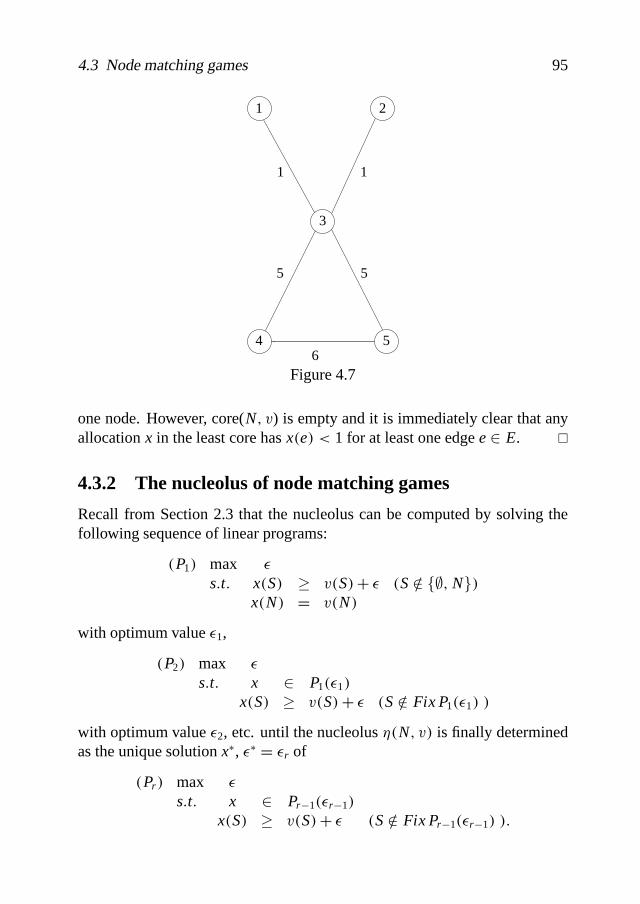
4.3 Node matching games 95
5
1
6
5
1
2
4
3
5
1
Figure 4.7
one node. However, core(N; v) is empty and it is immediately clear that anyallocationx in the least core hasx.e/ < 1 for at least one edgee∈ E. �
4.3.2 The nucleolus of node matching games
Recall from Section 2.3 that the nucleolus can be computed by solving thefollowing sequence of linear programs:
.P1/ max ž
s:t: x.S/ ≥ v.S/+ ž .S =∈ {∅; N}/x.N/ = v.N/
with optimum valuež1,
.P2/ max ž
s:t: x ∈ P1.ž1/
x.S/ ≥ v.S/+ ž .S =∈ Fix P1.ž1/ /
with optimum valuež2, etc. until the nucleolus�.N; v/ is finally determinedas the unique solutionx∗, ž∗ = žr of
.Pr / max ž
s:t: x ∈ Pr−1.žr−1/
x.S/ ≥ v.S/+ ž .S =∈ Fix Pr−1.žr−1/ /:
96 Matching games
By Theorem 4.9 (P1) is equivalent to. ˆP1/ in the sense that they define thesame set of optimal solutions. As we shall see, similar equivalent formulationscan be found for (Pk), k≥ 2. Define recursively
.ˆPk/ max ž
s:t: x ∈ ˆPk−1. ˆžk−1/
x.e/ ≤ w.e/+ ž1− ž .e∈ E.⋃D/;e =∈ Fix ˆPk−1. ˆžk−1/ /
x.e/ ≥ w.e/− ž1+ ž .e∈ E\E.⋃D/;e =∈ Fix ˆPk−1. ˆžk−1/ /
xi ≥ −ž1+ ž .i ∈ N; i =∈ Fix ˆPk−1. ˆžk−1/ /:
As before, let ˆžk denote the optimum value of (ˆPk) and define ˆPk.ž/ in theobvious way.
Theorem 4.10 We havežk = ˆžk and Pk.žk/ = ˆPk. ˆžk/ for k = 1; : : : ; r. In
particular, ˆP1. ˆž1/ ⊃ : : : ⊃ ˆPr = {x∗} defines the nucleolus�.N; v/.
Proof: For k = 1 the claim is equivalent to Theorem 4.9. We proceed by
induction onk. Assume thatžk−1 = ˆžk−1 andPk−1.žk−1/ = ˆPk−1. ˆžk−1/. Theinduction step amounts to show the following two things.
(i) Pk.ž/ ⊆ ˆPk.ž/ (implying that ˆžk ≥ žk) :
Let x ∈ Pk.ž/. Thenx ∈ P1.ž1/ = ˆP1. ˆž1/, so x satisfiesx ≥ 0, xi = xD −wD+wi ≤wi for all i ∈ D; D ∈D, andx.M/=w.M/+ ž1 for all M ∈M∗
D.
We first considere∈ E\E.⋃D) and show thatx.e/ ≥ w.e/− ž1+ ž unless
e∈ Fix ˆPk−1. ˆžk−1/ = Fix Pk−1.žk−1/. ChooseM ∈M∗D such thatM ∪ e is a
matching. (Existence follows from the fact that eachD ∈D is factor-critical.)
SinceM is fixed by ˆP1. ˆž1/ = P1.ž1/, it is fixed by ˆPk−1. ˆžk−1/. Hencee∈Fix ˆPk−1. ˆžk−1/ if and only if M ∪ e ∈ Fix ˆPk−1. ˆžk−1/. Since we assume
thate =∈ Fix ˆPk−1. ˆžk−1/, we haveM ∪ e =∈ Fix Pk−1.žk−1/ and thusx∈ Pk.ž/
implies x.M ∪ e/ ≥ w.M ∪ e/+ ž. Together withx.M/ = w.M/+ ž1 thisyieldsx.e/ ≥ w.e/− ž1+ ž.In the same way we can show thatxi ≥−ž1+ ž for a nodei =∈ Fix ˆPk−1. ˆžk−1/.
Next considere∈ E.⋃D/, saye∈ E.D/ for D ∈ D. We show thatx.e/ ≤
w.e/+ ž1− ž unlesse is already fixed byˆPk−1. ˆžk−1/ = Pk−1.žk−1/. Since

4.3 Node matching games 97
xi − wi = xj − w j for all i; j ∈ D, we conclude thatx.e/ − w.e/ is inde-pendent of the particular choice ofe∈ E.D/. Choose anyM ∈ M∗D and as-sume without loss of generality thate∈ M ∩ E.D/ is not fixed byPk−1.žk−1/.Sincex.M/ is fixed (tow.M/+ ž1), we conclude thatM\e =∈ Fix Pk−1.žk−1/.Hencex ∈ Pk.ž/ implies x.M\e/ ≥ w.M\e/ + ž. Together withx.M/ =w.M/+ ž1 we getx.e/ ≤ w.e/+ ž1− ž.
(ii) ˆPk.ž/ ⊆ Pk.ž/ (implying thatžk ≥ ˆžk):
Let x∈ ˆPk.ž/. Again this impliesx∈ ˆP1. ˆž1/, sox≥ 0, xi = xD−wD+wi ≤wi for all i ∈ D; D ∈ D andx.MD/ = w.MD/+ ž1 for all MD ∈M∗
D.
We are to show thatx.S/≥ v.S/+ ž for S⊂ N not yet fixed byPk−1.žk−1/=ˆPk−1. ˆžk−1/. Sincex ≥ 0, we may only considerS= N.M/ for M ∈ M.Furthermore, sincex.e/ ≥ w.e/ on E\E.
⋃D/, we may restrict ourselves
to M ⊆ E.⋃D/. Finally, sincexi = xD − wD +wi for all i ∈ D; D ∈ D;
x.M/−w.M/ only depends on|M ∩ D| for eachD ∈ D. So we may withoutloss of generality assume thatM ⊆ MD for someMD ∈ M∗
D. Assume thatM is not fixed byPk−1.žk−1/. SinceMD is fixed byPk−1.žk−1/, we concludethat MD\M is not fixed byPk−1.žk−1/. So at least somee∈ MD\M is not
fixed by Pk−1.žk−1/. Hencex ∈ ˆPk.ž/ implies x.e/ ≤ w.e/ + ž1− ž. Allother edgesf ∈ MD\M satisfy x. f / ≤ w. f / (as x ≤ w on
⋃D). Hence
x.MD/ = w.MD/+ ž1 impliesx.M/ ≥ w.M/+ ž as required. �
Clearly, the number of constraints in each linear program.ˆPk/ is bounded by
a polynomial in|N|. The size of the parametersˆžk .1= 1; : : : ; r / is boundedby a polynomial in< N; v > (cf. Remark 2.1). Then we can conclude that
Corollary 4.4 The nucleolus of a node matching game (N; v) can be com-puted in polynomial time. �
We end this section by giving an explicit formula for the nucleolus in casethe graph (N; E) with node weightingw satisfies some extra conditions. Firstconsider the following observation.
Proposition 4.4 Let i; j be two nodes in a component D∈ D that are notconnected. Let (N; v′) be the node matching game obtained from (N; v) byadding the edge.i; j/ to G. Then�.N; v′/ = �.N; v/.Proof: The proof is straightforward, noting the fact that for all allocations
x∈ P1.ž1/ = ˆP1. ˆž1/
xk−wk = xl −wl for all k; l ∈ D:

98 Matching games
So adding the edge (i; j) does not yield any new equations in the linear pro-
grams. ˆPk/ .k= 1; : : : ; r /. �
Now supposeT ∪⋃C is empty. Let
D = S1∪ : : : ∪ Sl
be the partition ofD such that all componentsD ∈ D with equal size|D|are in the same subcollectionSi, and |D| < |D′| for D ∈ Si, D′ ∈ S j and1≤ i < j ≤ l .
We say that a node weighting issymmetricif we can order the nodes in anytwo componentsD; D′ ∈ D with |D| = |D′| as i1; : : : ; i|D| and j1; : : : ; j|D|such that
wir = w jr .r = 1; : : : ; |D|/:
Below we give an expression for the nucleolus in caseT ∪⋃C is empty and
w is symmetric.
Theorem 4.11 Let T∪⋃C be empty and letw : N → R+ be symmetric.
Then the nucleolus of (N; v) is equal to the allocation x∗ ∈ RN given by
x∗i = wi −wD
min if i ∈⋃S1∪ : : : ∪
⋃Sk−1
wi − Þ if i ∈⋃Sk
wi if i ∈⋃Sk+1∪ : : : ∪
⋃Sl ;
where1 ≤ k ≤ l is taken as small as possible in such a way that a numberÞ ≥ 0 exists with the property that x∗ ∈ RN is of the form above, x∗ ≥ 0 andx∗.N/ = v.N/.Proof: First suppose core(N; v) is nonempty. Letx ∈ core(N; v). By Theo-rem 4.6 xi = 0 if i ∈ N is an isolated node. By Proposition 4.2xi = wi holdsfor all D ∈ D with |D| > 1. So core(N; v) contains exactly one allocation,which must be the nucleolus. ChooseÞ = 0. If a componentD ∈ S1 has size|D| > 1 then letk= 1. Otherwise letk= 2.
Suppose core(N; v) is empty. As a first step in computing the nucleolus we
have to determine the optimal valuež1 of .P1/ = . ˆP1/. Note that maximizingž comes down to maximizing∑
D∈D.|D| − 1/xD:

4.3 Node matching games 99
So we maximizexD on componentsD with |D| as large as possible in such a
way that the constraints of. ˆP1/ : x.N/ = v.N/; x= x; xD ≤ wD .D ∈ D/andx≥ 0, are met. Then it is clear that in this wayk has to be chosen as smallas possible such that the resulting vectorx∗ has
x∗i = wi −wDmin if i ∈
⋃S1∪ : : : ∪
⋃Sk−1
x∗i = wi if i ∈⋃Sk+1∪ : : : ∪
⋃Sl ;
and x∗.⋃Sk/ = x∗.N/− x∗.N\
⋃Sk/ such thatx∗i − wi = x∗j − w j for all
i; j ∈ D; D ∈ Sk and x∗.⋃Sk/ ≥
∑D∈Sk
.w.D/ − |D|wDmin/ (then x∗ ≥ 0).
Also the nucleolus is of the same form asx∗.
By Proposition 4.4 we may without loss of generality assume that eachD ∈Dis a complete graph. SupposeD; D′ ∈ Sk. Order the nodes ofD asi1; : : : ; i|D|and the nodes ofD′ as j1; : : : ; j|D| such that
wir = w jr .r = 1; : : : ; |D|/:
Recall that the nucleolus satisfiesSym. Define a permutation³ : N→ N asfollows:
³.k/ = j r if k= i r .r = 1; : : : ; |D|/
i r if k= j r .r = 1; : : : ; |D|/k otherwise:
Thenv³.S/ = v.S/ for all S⊆ N. If we want the nucleolus to be equal tox∗
then, according toSym, x∗ must be chosen such thatx∗ir = x∗jr for 1≤ r ≤ |D|.This implies that for alli ∈
⋃Sk x∗i = wi − Þ for some 0≤ Þ ≤ wi. �
4.3.3 Cardinality matching games
As mentioned before, cardinality matching games are a subclass of the classof node weight matching games with node weighting equal to a half for allnodes.
Below we assume that (N; v) is a cardinality matching game defined by agraph (N; E). Again T ⊆ N is the Tutte set satisfying the conditions (i) and(ii) in Theorem 4.4. Sincew ≡ 1
2 > 0, Theorem 4.8 reduces to the followingsimple observation (for a characterization, see also Deng, Ibaraki and Nag-amochi [1999]).

100 Matching games
Corollary 4.5 The cardinality matching game.N; v/ has nonempty core ifand only if|D| = 1 for all D ∈ D. �
Because all nodesi ∈ N have the same positive weightwi = 12, the setM∗
coincides with the setM∗. FurthermorewD = 12 for all D ∈ D. Then the
linear program. ˆP1/ describing the least core can be written as
.ˆP1/ max ž
s:t: xi = xD .i ∈ D; D ∈ D/xi ≤ 1
2 .i ∈⋃D/
x.e/ ≥ 1 .e∈ E\E.⋃D//
x.N/ = v.N/x.M/ ≥ |M|+ ž .M ∈M∗
D/x ≥ 0;
wherev.N/ = |⋃C|+ |T|+∑D∈D12.|D| − 1/. This way we have obtained
the characterization of the least core as presented in Kern and Paulusma [2000].Becausew ≡ 1
2 is symmetric, we can apply Theorem 4.11 (cf. Example 4.5).
Corollary 4.6 If T ∪⋃C is empty, then the nucleolus of (N; v) is equal to
the allocation x∗ ∈ RN given by
x∗i =
0 if i ∈
⋃S1∪ : : : ∪
⋃Sk−1
12 − Þ if i ∈
⋃Sk
12 if i ∈
⋃Sk+1∪ : : : ∪
⋃Sl ;
where1 ≤ k ≤ l is taken as small as possible in such a way that a numberÞ ≥ 0 exists with the property that x∗ ∈ RN is of the form above, x∗ ≥ 0 andx∗.N/ = v.N/. �

Chapter 5
Competition games
We consider a class of games related to sports competitions, in which variousteams play matches against each other in pairs according to a previously de-termined schedule. At some stage of the competition a team may try to bribesome other teams in order to win the competition. Those other teams form theplayer set in the competition game introduced in Section 5.1. The difficultyhere is deciding whether bribing yields the desired result or not. Therefore, inSection 5.2 we first try to solve the problem whether it is possible at all that atsome stage of a competition a certain team can end up with the highest finalscore. The computational complexity of this problem turns out to depend onthe way scores are allocated according to the outcome of a match. We deter-mine the complexity for all possible score allocation rules. In Section 5.3 wereturn to our competition game and give an algorithm to compute the value ofa coalition.
5.1 Introduction
Consider a sports competition like a national soccer league, in which all par-ticipating teams play against each other in pairs (matches) according to a pre-fixed schedule. Initially all teams have total score zero. When a team partic-ipates in a match, its total score is increased byÞ ∈ R if it loses the match,by þ ∈ R if the match ends in a draw, and by ∈ R if it wins the match. Wealways assume thatÞ ≤ þ ≤ and call the triple (Þ; þ; ) the rule (score al-location rule) of the competition. In case of a soccer competition, the formerFIFA rule was.Þ; þ; / = .0;1;2/, but this has been changed into the new
101

102 Competition games
rule .Þ; þ; / = .0;1;3/. Other sports like chess or draughts still use the rule.Þ; þ; / = .0;1;2/, while stratego, also a strategic board game, has as scoreallocation rule.Þ; þ; / = .0;1;6/.At some stage of the competition a team may ask whether it still has a (theo-retical) chance of “winning” the competition, i.e, ending up with the highestfinal total score. If this is possible it may try to bribe some other participatingteams. Here we assume that both teams have to be involved if the end resultof a match must be set to a draw and that in case of a win/loss match only thelosing team has to be bribed.
We use the following notations.N denotes the (finite)set of teamsparticipat-ing in the competition. The team in this set that wants to bribe its opponentsis denoted byt0. At a certain stage of the competition the position of eachteam in the ranking is determined by thecurrent score vector s∈ RN, wheresi is the current score of teami ∈ N . The set of remaining matches is denotedby M. It is possible that two matchesm1 andm2 in M have the same pair ofteams.i; j/ playing against each other. Thestate of a competitionis given bya triple.N; s;M/.
Definition 5.1 Given a rule (Þ; þ; ) and a state of a competition (N; s;M), acompetition game(N; v) consists of a setN = N\t0 and characteristic func-tion v : 2N→ R+ that is of the form
v.S/ ={v∗ if t0 wins the competition after bribingS0 otherwise;
wherev∗ ≥ 0 is called thebribeof the competition. �
Clearly, a valuev.S/ does not only depend on the state of the competition butalso on its rule. A coalitionS is called influential if v.S/ = v∗. In that casev.S/ can be interpreted as the price that is agreed by botht0 and coalitionSfor cheating the competition. If bribingSdoes not guaranteet0 to win, thent0 has no interest in coalitionSandv.S/ = 0. If another influential coalitionis cheaper, thent0 would not do business withS. Therefore, all prices are setequal to the same amountv∗.
Example 5.1 Consider some sports competition with rule.0;1;2/ and state.N; s;M/ given by the tables below.

5.2 The sports competition problem 103
teams scores
t0 10t1 9t2 6t3 3t4 2
remainingmatches
t0− t2t0− t3t3− t0t1− t4t4− t1
Then a competition game.N; v) is determined byN = {t1; t2; t3; t4} andv :2N→ R+ given by
v.S/ ={v∗ if t1 ∈ Sor t3 ∈ S0 otherwise:
�
Since we would have a trivial game ifv.N/= 0, we only consider competitiongames (N; v) with v.N/ = v∗ > 0. In those competitions teamt0 still hasa chance to achieve the highest final score. Then the question arises howdifficult it is to check whether this condition holds or not. In the next sectionwe solve this problem.
5.2 The sports competition problem
5.2.1 The model
In this section we determine the computational complexity of the problem
”Given a competition with state (N; s;M/ and rule (Þ; þ; ) has team t0 stilla chance to win the competition?”
To analyze this we may without loss of generality assume thatt0 wins all itsremaining matches, resulting in a final total scores0 for t0. The current scoresi of a teamti 6= t0 only has to be adjusted, ifti had to play againstt0 andÞ 6= 0. As we shall see later on, we may assumeÞ = 0. So we still denotethe (possibly adjusted) scores of the other teams bysi. The problem is now

104 Competition games
whether the teamsti 6= t0 can finish the remaining matches in such a waythat eachti collects at mostci := s0− si additional score points. (We permitthe situation thatt0 shares the first place in the final ranking with some otherteams.)
This can be modeled by a multigraphG= .V; E/, whose nodes correspondto teamsti 6= t0 and edges are in 1-1 correspondence with remaining matches.Each nodei ∈ V has capacityci ∈ R, as defined above. We represent theoutcome of a matche= .i; j/ by directing the edge from the winner to theloser (and leaving the edge undirected in case of a draw). This way we obtaina partially oriented graph, i.e., a graph with an edge set that contains bothdirected and undirected edges.
Because it will turn out that the computational complexity of our sports com-petition problem (SC) depends on the rule (Þ; þ; ) of the competition, wesubdivide our problem into the classes SC(Þ; þ; ).
Definition 5.2 SPORTS COMPETITION (SC(Þ; þ; ))
Instance: A multigraphG= .V; E/ and node capacitiesc∈ RV.
Question: CanG be partially oriented such that for each nodei ∈ V:
ÞŽ−.i /+ þŽ0.i /+ Ž+.i / ≤ ci ? (5.1)
Here, as usual,Ž+ and Ž− denote the outdegree and indegree of a node,whereasŽ0 denotes the number of incident unoriented edges. A partial ori-entation ofG satisfying the capacity constraints (5.1) is called asolutionofthe instance (G; c). �
Below we give an example of an instance of SC(0;1;2).
Example 5.2 Consider some sports competition with rule.0;1;2/ and state.N; s;M/ given by the tables below.
teams scores
t0 8t1 7t2 7t3 5t4 3
remainingmatches
t0− t2t1− t2t2− t1t1− t3t3− t4
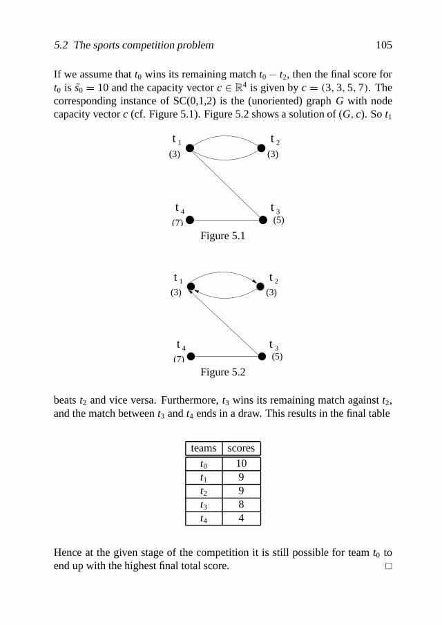
5.2 The sports competition problem 105
If we assume thatt0 wins its remaining matcht0− t2, then the final score fort0 is s0 = 10 and the capacity vectorc ∈ R4 is given byc= .3;3;5;7/. Thecorresponding instance of SC(0,1,2) is the (unoriented) graphG with nodecapacity vectorc (cf. Figure 5.1). Figure 5.2 shows a solution of (G; c). Sot1
t
4 t 3 t
2
(5)(7)
1 t
(3) (3)
Figure 5.1
t
4 t 3 t
2
(7) (5)
1 t
(3) (3)
Figure 5.2
beatst2 and vice versa. Furthermore,t3 wins its remaining match againstt2,and the match betweent3 andt4 ends in a draw. This results in the final table
teams scores
t0 10t1 9t2 9t3 8t4 4
Hence at the given stage of the competition it is still possible for teamt0 toend up with the highest final total score. �

106 Competition games
In the literature a simplified version of the sports competition problem (disal-lowing draws) is known. In that case the problem reduces to a flow problem,cf. Cook, Cunningham, Pulleyblank and Schrijver [1998] or the section be-low. As we shall see, however, the question becomes more interesting if drawsmay occur. Our main result, which has been proved independently by Bern-holt, Gulich, Hofmeister and Schmitt [1999], implies that in caseÞ < þ <
the problem is polynomially solvable if and only ifÞ + = 2þ (assumingP 6= NP). This means that for games like draughts and chess the problem ispolynomially solvable.
A lot of sports competitions, such as the FIFA soccer competitions, have theproperty that each participating team has to play the same number of matchesagainst every other team. We call this type of competitionsclosed. Wecan split a class SC(Þ; þ; ) into a subclass of closed competitions with rule(Þ; þ; ) and a subclass ofopen competitions, where the property mentionedabove does not hold (e.g., large one- or two-day open tournaments). A cou-ple of years ago the FIFA exchanged the rule (0;1;2) for the current rule(0;1;3). Therefore we are especially interested in the computational com-plexity of SC restricted to closed competitions. We show that the complexitydoes not change under this restriction. This implies that for soccer competi-tions, by changing the score allocation rule into the rule.Þ; þ; / = .0;1;3/,the problem has becomeNP-complete. Also for stratego competitions theproblem isNP-complete.
We end our introduction with the following simple observation. Given aninstance (G; c) of SC(Þ; þ; ), we can derive an equivalent instance (G; c′) ofSC(0; þ− Þ; − Þ) by settingc′i := ci − ÞŽ.i /. (Here,Ž refers to the degreein G.) So with respect to computational complexity of SC(Þ; þ; ) we mayalways assume that (Þ; þ; ) is normalized, in the sense thatÞ = 0≤ þ ≤ .
5.2.2 Complexity results
Our main result (cf. Kern and Paulusma [2001]) completely determines thecomputational complexity of the sports competition problem. In cases whereSC(Þ; þ; ) turns out to beNP-complete we prove this by reduction from3-dimensional matching. This is a well-knownNP-complete problem (cf.Garey and Johnson [1979]).

5.2 The sports competition problem 107
3-DIMENSIONAL MATCHING (3DM)
Instance: three disjoint setsX;Y;W with the same number of elementsq anda subsetR⊆ X× Y×W.
Question: DoesR contain a (3-dimensional) matching, i.e., is there a subsetof triplesR′ ⊆ Rsuch thatR′ covers each element ofX∪Y∪W exactly once?
(In Bernholt, Gulich, Hofmeister and Schmitt [1999]NP-completeness isproved by a reduction from theNP-complete problem 3-SATISFIABILITY,see Garey and Johnson [1979].)
Theorem 5.1 SC(Þ; þ; ) is polynomially solvable in each of the followingthree cases:
(i) Þ = þ(ii) þ =
(iii) Þ+ = 2þ.
In all other cases the problem isNP-complete.
Proof: First recall that we may assume that (Þ; þ; ) is normalized, soÞ = 0.(Note that normalization does not affect cases (i)-(iii).)Case (i)is then trivial.Indeed, an instance (G; c) has a solution if and only ifc≥ 0. (Leave all edgesunoriented.)
In all other cases we haveþ > 0. By scaling we may assume thatþ = 1.(Divide þ; as well asc by þ.)
Case (ii) þ = = 1 (corresponding with the exclusion of draws).
Consider an instance given byG= .V; E/ andc ∈ RV. Construct a directedbipartite graph with node setsV and E and arcs linking eachi ∈ V to alledges inE incident with i in G. Then add an additional sources and sinkt as indicated in Figure 5.3. The arcs froms to V all get lower capacity 0and upper capacitybcic .i ∈ V/. The arcs fromV to E get lower capacity0 and upper capacity 1. The arcs fromE to t get lower capacity and uppercapacity 1. The resulting network has a feasibles-t flow x ∈ R|V|+3|E| if andonly if our instance (G; c) has a solution. Indeed, as all capacities are integral,a feasible flow may also be assumed to be integral (cf. Theorem 1.4). Givenan integral feasible flow we can interpret an arc (i; .i; j/) from V to E that

108 Competition games
..
...
....
(i,j)
s t
j
iV
E
Figure 5.3
carries 1 unit of flow asi winning the matche= .i; j/ and conversely (cf.also Cook, Cunningham, Pulleyblank and Schrijver [1998]).
Case (iii) þ = 1; = 2 (ancient FIFA rule).
This can be solved similarly. In the network of Figure 5.3 we simply redefinethe upper capacities of all arcs fromV to E to be 2. The lower and uppercapacities of arcs fromE to t are also set to 2. Again, feasible integral flowsare in 1-1 correspondence with solutions of our instance (G; c). Each nodee∈ E in our network has two incoming arcs that carry a total flow of 2 units,distributed as 2 : 0 or 1 : 1, corresponding to a win/loss match or a draw.
To prove the last part of the theorem we make a distinction between the case“þ = 1; > 2” and “þ = 1;1< < 2”. Since we can guess an outcome ofthe remaining matches and compute the final scores, in both cases SC(Þ; þ; )is a member ofNP.
Case (iv)þ = 1; > 2.
We proveNP-completeness by reduction from 3DM. Suppose|X| = |Y| =|W| = q and R⊆ X× Y×W is given. We are to determine whetherR con-tains a matchingR′ ⊆ R. Assume without loss of generality that each elementz∈ X∪Y∪W actually occurs in some tripler ∈ R. We writez∈ r to indicatethatz occurs inr ∈ R.

5.2 The sports competition problem 109
Given R⊆ X×Y×W, we construct a graphG= .V; E/ as follows. We firstmake one copy of each elementz∈ X∪Y∪W for each occurrence ofz in R,i.e., we define
X := {.x; r / | x∈ X; r ∈ R; x∈ r}Y := {.y; r / | y∈ Y; r ∈ R; y∈ r}W := {.w; r / | w ∈W; r ∈ R; w ∈ r}:
Construct a graphG= .V; E/with node setV = X∪Y∪W∪ X∪ Y∪ W∪ Rand edges as defined by the incidence relations in a straightforward way, i.e.,
E = {.x; .x; r // | .x; r / ∈ X}∪ {.y; .y; r // | .y; r / ∈ Y}∪ {.w; .w; r // | .w; r / ∈ W}∪ {.r; .x; r // | .x; r / ∈ X}∪ {.r; .y; r // | .y; r / ∈ Y}∪ {.r; .w; r // | .w; r / ∈ W} (cf. Figure 5.4 below):
Next define node capacitiesc∈ RV as follows:
...R
...r
...
W
(w,r)
w
W
...
...X
(x,r)
x
X(y,r)
...Y
Y
y
...
Figure 5.4

110 Competition games
c ≡ 1 on X∪ Yc ≡ 1+ on X∪ Yc ≡ max{ ;3} on Rc ≡ 1 onWc ≡ .Ž− 1/+ 1 onW:
(Again,Ž refers to the degree function ofG.)
We claim that this instance (G; c) has a solution if and only ifR contains amatching.
“⇐” SupposeR′ ⊆ R is a matching. Define a corresponding partial ori-entation ofG as follows. For eachw ∈ W choose the uniquer ′ ∈ R′ with.w; r ′/ ∈ W. We leave the edge.w; .w; r ′// unoriented and orient all otheredges fromw to W. This way the capacity constraints ofw are met. For eachr ′ = .x; y; w/ ∈ R′ we orient the edge.r ′; .w; r ′// from r ′ towards.w; r ′/ andthe edges.r ′; .x; r ′// and.r ′; .y; r ′// from X respectivelyY towardsr ′. Alledges incident withr ∈ R\R′ remain unoriented. This way we ensure that thecapacity constraints onW and R are respected. Finally, orient all edges be-tweenX andX from X towardsX except those that correspond to an elementin R′ (these remain unoriented). This way the capacity constraints forX andX are met. We orient edges betweenY andY in the same way. This partialorientation gives a solution of the instance (G; c).
”⇒” Conversely, suppose we are given a partial orientation ofG respectingthe capacity constraints. The latter imply that forx ∈ X we haveŽ−.x/ ≥Ž.x/− 1 andŽ+.x/ = 0. We may assume without loss of generality that ac-tually Ž−.x/ = Ž.x/− 1. (Otherwise, i.e., ifŽ−.x/ = Ž.x/, pick an arbitraryedge incident withx and make it unoriented. The modified orientation willstill respect all capacity constraints.) A similar argument holds for elementsy ∈ Y. Nodes inX have degree 2. In view of their capacity bound 1+ , wemay assume without loss of generality that each.x; r / ∈ X hasŽ0 = 1 andŽ+ = 1. (Otherwise, again modify the solution without violating the capacityconstraints.) As eachx∈ X hasŽ−.x/= Ž.x/−1 andŽ0.x/= 1, we concludethat
• There are exactly|X| arcs directed fromX to R. Moreover, if..x; r /; r / isdirected towardsr and..x′; r ′/; r ′/ is directed towardsr ′, thenx 6= x′.
The same holds for the directed arcs fromY to R.

5.2 The sports competition problem 111
Arguing similarly for nodes inW, we find that eachw ∈ W has without lossof generalityŽ+.w/ = Ž.w/− 1 andŽ0.w/ = 1. (Otherwise modify the ori-entation such thatw actually uses its full capacity.) Nodes inW have degree2 and capacity bound 1. Then we may without loss of generality assume thatthese nodes haveŽ0 = 1 andŽ− = 1. The above implies that
• There are exactly|W| arcs directed fromR towardsW. Moreover, if theedge.r; .w; r // is directed fromr towards.w; r / and.r′; .w′; r ′// is directedfrom r ′ towards.w′; r ′/, thenw 6= w′.Finally, the capacity constraints onR imply that a noder ∈ Rcan haveŽ+ ≥ 1only if Ž− ≥ 2. From this and the above observations, it is straightforward tocheck that
R′ = {r ∈ R | Ž+.r / = 1}
actually is a matching.
Case (v) þ = 1< < 2.
Again, we proveNP-completeness by reduction from 3DM. In the graphGof Figure 5.4 we replace the node capacitiesc ∈ RV by node capacitiesc asfollows:
c ≡ .Ž− 1/+ 1 on X∪ Yc ≡ 1 on X∪ Yc ≡ max{2 ;3} on Rc ≡ 1+ on Wc ≡ 1 onW:
Analogously to Case (iv) one can prove that the instance (G; c) has a solutionif and only if R contains a matching. �
Theorem 5.1 is related to the class of all possible sports competitions. Re-call that this class contains both closed competitions and open competitions.Because a lot of sports competitions such as the FIFA soccer competitionsare closed, we want to determine the computational complexity of our sportscompetition problem restricted to this kind of competition as well. Obviouslyfor score allocation rules, for which the general sports competition can besolved in polynomial time, the problem for closed competitions can be solvedefficiently. The following theorem shows that also for the other rules the com-putational complexity does not change. We call the number of times that eachteam plays against every other team theorder² of the competition.

112 Competition games
Theorem 5.2 Consider a class of closed competitions with fixed rule (Þ; þ; )and fixed order². Then the problem of determining whether at a given stagea certain team can win the competition isNP-complete if
Þ < þ < and Þ+ 6= 2þ:
Proof: For the rule (Þ; þ; ) we again assumeÞ = 0 andþ = 1. If > 2 thenwe only have to show that for the instance (G; c), as defined in Case (iv) ofthe proof of Theorem 5.1, there exists a closed competition of order² with astate (N; s;M) such that (G; c) is obtained from this state. If 1< < 2 wehave to find an appropriate competition for instance.G; c) of Case (v) in theproof of Theorem 5.1. Because such a closed competition can be constructedin the same way we only prove the case > 2.
Hence let > 2 and consider (first) the case² = 1.
In Case (iv) of the proof of Theorem 5.1 we have a graphG= .V; E/ withnode setV = X∪Y∪W∪ X∪ Y∪ W∪ Rand edges as defined in Figure 5.4.Furthermore, the node capacitiesc∈ RV are given by
c ≡ 1 on X∪ Yc ≡ 1+ on X∪ Yc ≡ max{ ;3} on Rc ≡ 1 onWc ≡ .Ž− 1/+ 1 onW:
We construct a competition that contains (besides teamt0) the teams corre-sponding withV and, in addition, the following teams:
� for all x∈ X a setH.x/ of Ž.x/− 1 teams;
� for all y∈ Y a setH.y/ of Ž.y/− 1 teams;
� for all w ∈ W a setH.w/ of one team;
� for all r ∈ R a setH.r / of two teams.
Let H1 denote the collection of all teams as defined above ,i.e.,
H1 =⋃x∈X
H.x/∪⋃y∈Y
H.y/∪⋃w∈W
H.w/∪⋃r∈R
H.r /:

5.2 The sports competition problem 113
BesidesH1, we add a set of teamsH2 of size |H2| sufficiently large (as ex-plained later). Then the set of teams in this competition is
N = V ∪ H1∪ H2∪ {t0}:
The total set of matches between pairs of teams inN has size12|N|.|N| − 1/.
We want the set of remaining matchesM to correspond exactly with the setof edgesE and a current score vectors in such a way that every teami ∈ Vmay collect at mostci additional score points. For this purpose we define thefollowing outcomes of matches not inE.
� Teamt0 wins all its matches against teams inH2, its matches against teamsin V all end in a draw, andt0 loses all its matches against the teams inH1.
� Matches between teams inV that do not correspond with an edge inE endin a draw.
� Every teami ∈ X ∪ Y ∪ W wins all its matches against teams inH2, itsmatches against teams inH.i / all end in a draw, andi loses all matches againstteams inH1\H.i /.
� Every teami ∈ W wins |H2| − Ž.i /+ 1 matches against teams inH2, allits other matches against teams inH2 end in a draw, andi loses all matchesagainst teams inH1.
� Every teami ∈ X ∪ Y wins |H2| − 1 matches against teams inH2, its re-maining match inH2 ends in a draw, andi loses all matches against teams inH1.
� If ≤ 3, then every teami ∈ R wins all matches against teams inH2 andloses its matches againstH.i /. If > 3, then every teami ∈ Rwins |H2| − 1matches against teams inH2 and its remaining match inH2 plus the matchesagainst the teams inH.i / end in a draw. In both casesi loses its matchesagainst teams inH1\H.i /.
� Every teami ∈ H1 loses all matches against teams inH2. Matches betweenteams inH1 all end in a draw.
�Matches between teams inH2 end in a draw.
This way t0 has no remaining matches ands0 = s0 = |V|+ |H2|. Further-more we have made sure thatci = s0− si holds for all teamsti ∈ V.

114 Competition games
Because all teams inH1 ∪ H2 have no remaining matches, they will corre-spond with isolated nodes if they are added toG. So we have a set of remain-ing matchesM in 1-1 correspondence with edges inE. However, we still haveto check that teams inH1∪ H2 do not have a final score greater thans0. Forall i ∈ H1 we deduce that its score
si ≤ |H1|+ + + .|V| − 1/ = |H1|+ + |V|;and for alli ∈ H2 we have
si ≤ |H2|+ |H1|+ |V|:It is easy to see that both upper bounds will be smaller than|V|+ |H2| = s0
provided thatH2 is sufficiently large. Hence we have constructed a competi-tion with a state.N; s;M/ such that (G; c) is obtained from this state (omittingthe isolated nodes).
Above we have assumed that each team plays exactly one time against allother teams. For a class of competitions with order² > 1 we let²−1 matchesbetween every pair of teams end in a draw. Then we use the same constructionas in the case² = 1. �
Theorem 5.2 implies that for soccer competitions with the current FIFA rule(0;1;3) and order for instance 2 or 4 it has indeed becomeNP-complete todecide whether at a given stage a certain soccer team wins the competition.
5.2.3 Related problems
Examining the proof of Theorem 5.1 we see that the network model we usedfor solving cases (ii) and (iii) of our main theorem does not apply for cases inwhich the rule (Þ; þ; ) has the property thatÞ < þ < andÞ+ 6= 2þ. Takefor instance the rule.Þ; þ; / = .0;1;3/. If we increase the upper capacitiesto 3 on all arcs fromV to E and fromE to t in the network of Figure 5.3, thena feasible flow does no longer necessarily represent a solution of our instance.(A total flow of 2 entering a nodee= .i; j/ ∈ E distributed as 2 : 0 on thetwo entering arcs does not correspond to a win/loss or a draw.) If we ”repair”this by introducing a ”capacity gap” ]1;3[ on all arcs fromV to E we geta flow problem with capacity gaps, which again nicely describes our sportscompetition problem. So as a consequence of our result, the following classof problems is alsoNP-complete.

5.2 The sports competition problem 115
Definition 5.3 FLOWS WITH CAPACITY GAPS (FCG)
Instance: A digraphD = .V; A/ with sources and sinkt and for each arca ∈ A two disjoint capacity intervalsI1.a/ = [c1.a/; c2.a/] and I2.a/ =[c3.a/; c4.a/] .ci.a/ ∈ Z; i = 1; : : : ;4/.
Question: Does a (integral)s-t flow x ∈ ZA exist with x.a/ ∈ I1.a/ ∪ I2.a/.a ∈ A/? �
Corollary 5.1 FCG isNP-complete. �
As to sports competitions, we would like to remark that also other questionscan be treated in the same way. For example ”Is there a chance that teamt0 ends up with the lowest final score?” turns out to be of exactly the samecomplexity as SC: Assume thatt0 has a current total scores0 and loses allremaining matches. This results in a current total scoresi for all other teamsti 6= t0. The question is now whether the teamsti 6= t0 can finish the remainingmatches in such a way that eachti collectsat least ci := s0 − si additionalscore points. Again we model this by a multigraphG= .V; E/ whose nodescorrespond to teamsti 6= t0 and edges are in 1-1 correspondence with remain-ing matches. Each nodei ∈ V has a (lower) capacityci ∈ R. Our “reverse”sports competition problem (RSC) can now be formulated as follows.
Definition 5.4 REVERSE SPORTS COMPETITION (RSC(Þ; þ; ))
Instance: A multigraphG= .V; E/ and node capacitiesc∈ RV.
Question: CanG be partially oriented such that for each nodei ∈ V:
ÞŽ−.i /+ þŽ0.i /+ Ž+.i / ≥ ci ? (5.2)�
It is easy to see that fori ∈ V, (5.2) is equivalent to
. − þ/Ž0.i /+ . − Þ/Ž−.i / ≤ Ž.i /− ci :
Hence an instance.G; c/ of RSC(Þ; þ; ) corresponds to an instance.G; Ž−c/ of SC(0; − þ; − Þ), and the corollary below immediately follows fromTheorem 5.1.
Corollary 5.2 RSC(Þ; þ; ) is polynomially solvable in each of the followingthree cases:
(i) Þ = þ
116 Competition games
(ii) þ = (iii) Þ+ = 2þ.
In all other cases the problem isNP-complete. �
Questions such as ”Is there a chance thatt0 ends up being one of the threeteams that have the three lowest final scores?” can also be treated in a similarway. Again, assume thatt0 has a current total scores0 and loses all remainingmatches. Choose two teamsti; t j 6= t0, and letti and t j lose their remainingmatches against teamstk .k 6= 0; i; j/. (Choose, if necessary, an arbitraryoutcome for the matches betweenti and t j.) These outcomes result in finaltotal scoress0 = s0, si and sj, and current total scoressk for all other teamstk .k 6= 0; i; j/. If it is possible that the teamstk .k 6= 0; i; j/ can finish theremaining matches in such a way that eachtk collects at leastck := s0− sk
additional score points, thent0 can indeed end up being one of the three lowestteams. If this is not possible for any pairti; t j, thent0 can never end up beingone of the three lowest teams. So one has to solve at most1
2|N|.|N| − 1/problem instances in RSC(Þ; þ; ). Hence also this question is of the samecomplexity as SC.
5.3 Competition games
Consider a competition game (N; v) obtained from a sports competition withstate (N; s;M) and rule (Þ; þ; ). Clearly computing the valuev.N/ comesdown to solve the corresponding instance.G; c/ of SC(Þ; þ; ). Below wegive an algorithm for computing the other valuesv.S/ .S 6= N/. Denotethe set of remaining matches of teamti by Mi. For S⊆ N let GS= .V; E/be the multigraph whose nodes correspond with the teams inS and whoseedges are in 1-1 correspondence with the remaining matches between teamsin S. In step (1) of the algorithm we assume that, after bribing,t0 will winits remaining matches against teams inS. However, in our modelt0 will onlybribe a coalitionS if it has an absolute guarantee on winning the competition.Because there is a probability thatt0 loses its matches inM against teamsoutsideS, we reward these kind of matches only withÞ points resulting ina lower bounds0 on its final total score. Obviously there is no guarantee onwinning, if it is possible for a team outsideS to achieve a higher final scorethan s0. If this situation cannot occur, we proceed with step (4). Recall thatwe assume that both teams have to be involved if the end result of a match

5.3 Competition games 117
must be set to a draw and that in case of a win/loss match only the losingteam has to be bribed. Under this assumption we let every team inS lose itsremaining matches against teams outsideS. Then it remains to check if thecorresponding instance of SC(Þ; þ; ) has a solution or not.
Algorithm COMP :
(1) Compute the final total scores0 for t0
s0 := s0 + Þ|{m∈ M0 | m= .t0; ti / with ti =∈ S}|
+ |{m∈ M0 | m= .t0; ti / with ti ∈ S}|:
(2) Compute the highest final scores that a teamti =∈ Smight achieve
s := max{si + |Mi| | ti =∈ S}:
(3) IF s0 < s THEN outputv.S/ = 0 and STOP.
(4) Adjust the current scoresi for each teamti ∈ S
si := si + Þ|{m∈ Mi | m= .ti ; t j / with t j ∈ N\S}| .ti ∈ S/:
(5) Compute the amountci of additional score points that each teamti ∈ Smay collect by
ci := s0− si .ti ∈ S/:
(6) Solve the instance (GS; c/ of SC(Þ; þ; ).
(7) IF the answer for (GS; c) is “yes” THEN outputv.S/ := v∗ OTH-ERWISE outputv.S/ := 0. STOP.
The computational complexity of the algorithm depends on the complexity ofsolving an instance of SC(Þ; þ; ). COMP is a polynomial time algorithm ifand only if SC(Þ; þ; ) is polynomially solvable.
Let N∗ denote the set ofindispensable teams, which contains all teams thathave to be included in any coalitionS that is bribed byt0. Because obviously

118 Competition games
v.S/ ≤ v.T/ for all S⊆ T ⊆ N, we have
N∗ := {i ∈ N | v.N\i / = 0}:
Note thatN∗ can be computed in polynomial time if the corresponding sportscompetition problem SC(Þ; þ; ) is polynomially solvable.
The following result gives an easy characterization of the core of a competi-tion game.
Theorem 5.3 Let (N; v) be a competition game withv.N/ = v∗. If N∗ isempty, then core(N; v) is empty. Otherwise
core.N; v/ = {x∈ I .N; v/ | x.N∗/ = v∗}:Proof: First supposeN∗ = ∅. Thenv.N\i / = v∗ for all i ∈ N. So if x ∈ RN
were in the core, then
|N|v∗ ≤∑i∈N
x.N\i / = .|N| − 1/x.N/;
implying x.N/ > v∗, a contradiction.
SupposeN∗ 6= ∅. Thenv.S/ = 0 if N∗\S is nonempty. Hence any positiveallocationx∈ RN with x.N∗/ = v∗ is a core vector.
Now supposex ∈ core.N; v/. Thenx ≥ 0 andx.N/ = v∗. If N∗ = N weare finished. Supposei =∈ N∗. Then we deduce fromx.N\i / ≥ v.N\i / = v∗,x≥ 0 andx.N/ = v∗ thatxi = 0. �
In Example 5.1v.N\i / = v∗ for all i ∈ N. HenceN∗ and core(N; v) areempty. The example below shows a competition game with a nonempty core.
Example 5.3 Consider a competition with rule.0;1;2/ and state.N; s;M/given by the tables below.
teams scores
t0 10t1 13t2 6t3 5t4 0
remainingmatches
t0− t2t0− t3t1− t4

5.3 Competition games 119
The competition game.N; v) is determined byN = {t1; t2; t3; t4} and v :2N→ R+ given by
v.S/ ={v∗ if S= {t1; t2; t3} or S= N0 otherwise:
ThenN∗ = {t1; t2; t3} and
core.N; v/ = {x∈ RN | x1+ x2+ x3 = v∗; x4 = 0 andx≥ 0}:
�
In the next theorem we prove that the Shapley value of a competition game(N; v) can easily be computed ift0 only has to bribe the indispensable teams.
Theorem 5.4 Let (N; v) be a competition game with N∗ 6= ∅. If v.N∗/ = v∗,then the Shapley value� is given by
�i.N; v/ =
v∗
|N∗| if i ∈ N∗
0 otherwise:
Proof: (i) Supposei; j ∈ N∗. Then
v.S∪ i / = 0= v.S∪ j/ for all S⊆ N\{i; j}:
By Theorem 2.4 we know that the Shapley value satisfiesSym. Now define apermutation³ : N→ N as follows:
³.k/ = j if k= i
i if k= jk otherwise:
It follows thatv³.S/ = v.S/ for all S⊆ N. Then, according toSym,
�i.N; v/ = � j.N; v/ for all i; j ∈ N∗: (5.3)
Also, by Theorem 2.4 the Shapley value satisfiesDum. Supposek =∈ N∗. Firstnote thatv.N∗/ = v∗ andv.T/ ≤ v.S/ for all T ⊆ S imply thatv.S/ = v∗ ifN∗ ⊆ S. Thenv.S/− v.S\k/ = 0= v.k/ for all S⊆ N. Sok is a dummy in.N; v). By propertyDumwe have
�k.N; v/ = 0 for all k ∈ N\N∗: (5.4)

120 Competition games
(5.3) and (5.4) imply that
�i.N; v/ =
v∗
|N∗| if i ∈ N∗
0 otherwise:
�
Note that the Shapley value as defined above is a core allocation. However,the following example makes clear that in casev.N∗/ = 0 the Shapley valueis not necessarily of this form.
Example 5.4 We consider a competition with rule.0;1;2/ and state.N; s;M/given by the tables below.
teams scores
t0 8t1 7t2 7t3 5t4 1
remainingmatches
t0− t3t0− t4t1− t3t3− t1t2− t3t3− t2
Then the competition game (N; v) is defined by set of teamsN= {t1; t2; t3; t4}and characteristic functionv given by
v.S/ ={v∗ if t3 andt4 in Sor S= {t1; t2; t3}0 otherwise:
HenceN∗ = {t3}. Sincev.t3/ = 0, Theorem 5.4 cannot be applied. Comput-ing the Shapley value yields�1 = �2 = 1
12v∗; �3 = 7
12v∗ and�4 = 3
12v∗. Note
that the Shapley value of this competition game is not a core allocation.�
Also with respect to the problems mentioned in the previous section (e.g.,RSC) we can define similar competition games, wheret0 tries to bribe someother teams. Furthermore, our model can be extended by letting the valuev.S/ depend on the (size of) coalitionS or by including some other teamsthat also want to win the competition by means of bribing.

Bibliography
AARTS, H. [1994], Minimum Cost Spanning Tree Games and Set Games,Ph.D. thesis, University of Twente, Enschede, the Netherlands.
BERNHOLT, T., A. GULICH, T. HOFMEISTER, AND N. SCHMITT [1999],Football elimination is hard to decide under the 3-point-rule, in:M. Kutylowski, L. Pacholski, and T. Wierzbicki (eds.),MathematicalFoundations of Computer Science 1999, Lecture Notes in ComputerScience 1672, 410–418.
BILBAO , J.M. [2000], Cooperative Games on Combinatorial Structures,Kluwer Academic, Norwell, Massachusetts.
BIRD, C.G. [1976], On cost allocation for a spanning tree. a game theoreticapproach,Networks6, 335–350.
BONDY, J.A.,AND U.S.R. MURTY [1976],Graph Theory with Applications,Macmillan, London and Elsevier, New York.
COOK, S.A. [1971], The complexity of theorem-proving procedures,Pro-ceedings of the Third Annual ACM Symposium on Theory of Computing,ACM, New York, 151–158.
COOK, W.J., W.H. CUNNINGHAM , W.R. PULLEYBLANK , AND A. SCHRI-JVER [1998], Combinatorial Optimization, John Wiley & Sons, NewYork.
DAVIS, M., AND M. M ASCHLER [1965], The kernel of a cooperative game,Naval Research Logistics Quarterly12, 223–259.
DENG, X., T. IBARAKI , AND H. NAGAMOCHI [1999], Algorithmic aspectsof the core of combinatorial optimization games,Mathematics of Op-erations Research24, 751–766.
DENG, X., AND C.H. PAPADIMITRIOU [1994], On the complexity ofcooperative game solution concepts,Mathematics of OperationsResearch19, 257–266.
DRIESSEN, T.S.H. [1991], A survey of consistency properties in cooperative
121

122 Bibliography
game theory,SIAM Review33, 43–59.DRIESSEN, T.S.H., AND D. PAULUSMA [2001], Two extensions of the
Shapley value for cooperative games,Mathematical Methods ofOperations Research53, 35–49.
EDMONDS, J. [1965a], Maximum matching and a polyhedron with 0;1-vertices,Journal of Research of the National Bureau of Standards Sec-tion B69B, 125–130.
EDMONDS, J. [1965b], Paths, trees, and flowers,Canadian Journal of Math-ematics17, 449–467.
EVANS, R.A. [1996], Value, consistency, and random coalition formation,Games and Economic Behavior12, 68–80.
FAIGLE, U., AND W. KERN [1992], The Shapley value for cooperativegames under precedence constraints,International Journal of GameTheory21, 249–266.
FAIGLE, U., AND W. KERN [1993], On some approximately balanced com-binatorial cooperative games,ZOR - Methods and Models of OperationsResearch38, 141–152.
FAIGLE, U., W. KERN, S.P. FEKETE, AND W. HOCHSTATTLER [1997], Onthe complexity of testing membership in the core of min-cost spanningtree games,International Journal of Game Theory26, 361–366.
FAIGLE, U., W. KERN, S.P. FEKETE, AND W. HOCHSTATTLER [1998],The nucleon of cooperative games and an algorithm for matchinggames,Mathematical Programming83, 195–211.
FAIGLE, U., W. KERN, AND J. KUIPERS[1998a], Computing the nucleolusof min-cost spanning tree games isN P-hard, International Journal ofGame Theory27, 443–450.
FAIGLE, U., W. KERN, AND J. KUIPERS [1998b], An efficient algorithmfor nucleolus and prekernel computation in some classes of TU-games,Memorandum 1464, University of Twente, Enschede, the Netherlands.
FAIGLE, U., W. KERN, AND D. PAULUSMA [2000], Note on the compu-tational complexity of least core concepts for min-cost spanning treegames,Mathematical Methods of Operations Research52, 23–38.
GALLAI , T. [1963], Kritische Graphen II,A Magyar Tudomanyos AkademiaMatematikai Kutato Intezetenek Kozlemenyei8, 373–395.
GALLAI , T. [1964], Maximale Systeme unabh¨angiger Kanten,A MagyarTudomanyos Akademia Matematikai Kutato Intezetenek Kozlemenyei9,401–413.
GAREY, M.R., AND D.S. JOHNSON [1979], Computers and Intractability:

Bibliography 123
A Guide to the Theory of N P-Completeness, Freeman, San Francisco,California.
GILLIES, D.B. [1959], Solutions to general non-zero-sum games, in: A.W.Tucker and R.D. Luce (eds.),Contributions to the Theory of Games IV,Annals of Mathematics Studies 40, Princeton University Press, Prince-ton, New Jersey, 47–85.
GRANOT, D., AND F. GRANOT [1992], On some network flow games,Math-ematics of Operations Research17, 792–841.
GRANOT, D., F. GRANOT, AND W.R. ZHU [1998], Characterization sets forthe nucleolus,International Journal of Game Theory27, 359–374.
GRANOT, D., AND G. HUBERMAN [1981], Minimum cost spanning treegames,Mathematical Programming21, 1–18.
GRANOT, D., AND G. HUBERMAN [1984], On the core and nucleolus ofminimum cost spanning tree games,Mathematical Programming29,323–347.
GRANOT, D., M. MASCHLER, G. OWEN, AND W.R. ZHU [1996], The ker-nel/nucleolus of a standard tree game,International Journal of GameTheory25, 219–244.
GROTSCHEL, M., L. LOVASZ, AND A. SCHRIJVER [1981], The ellipsoidmethod and its consequences in combinatorial optimization,Combina-torica 1, 169–197, [corrigendum: Combinatorica 4 (1984), 291-295].
GROTSCHEL, M., L. LOVASZ, AND A. SCHRIJVER [1993], GeometricAlgorithms and Combinatorial Optimization(Second ed.), Springer-Verlag, Berlin.
HOFFMAN, A.J., AND J.B. KRUSKAL [1956], Integral boundary points ofconvex polyhedra, in: H.W. Kuhn and A.W. Tucker (eds.),LinearInequalities and Related Systems, Annals of Mathematics Studies 38,Princeton University Press, Princeton, New Jersey, 223–246.
KERN, W., AND D. PAULUSMA [2000], Matching games: the least core andthe nucleolus, Memorandum 1541, University of Twente, Enschede, theNetherlands.
KERN, W., AND D. PAULUSMA [2001], The new FIFA rules are hard: com-plexity aspects of sports competitions,Discrete Applied Mathemat-ics108, 317–323.
KHACHIYAN , L.G. [1979], A polynomial algorithm in linear programming,Soviet Mathematics Doklady20, 191–194.
KONIG, D. [1931], Graphok ´es matrixok,Matematikaies Fizikai Lapok38,116–119, (Hungarian).

124 Bibliography
KRUSKAL, J.B. [1956], On the shortest spanning subtree of a graph and thetraveling salesman problem,Proceedings of the American Mathemati-cal Society7, 48–50.
KUIPERS, J. [1996], A polynomial time algorithm for computing the nucle-olus of convex games, Report M 96-12, Maastricht University, Maas-tricht, the Netherlands.
LOVASZ, L., AND M.D. PLUMMER [1986], Matching Theory, North-Holland Mathematics Studies 121, North-Holland, Amsterdam.
MASCHLER, M., B. PELEG, AND L.S. SHAPLEY [1979], Geometric proper-ties of the kernel, nucleolus, and related solution concepts,Mathematicsof Operations Research4, 303–338.
MEGIDDO, N. [1978], Computational complexity of the game theory ap-proach to cost allocation for a tree,Mathematics of Operations Re-search3, 189–196.
MICALI , S., AND V.V. VAZIRANI [1980], AnO.V 12 E/ algorithm for find-
ing maximum matching in general graphs,21st Annual Symposium onFoundations of Computer Science, IEEE, New York, 17–27.
NEMHAUSER, G.L., AND L.A. WOLSEY [1999], Integer and CombinatorialOptimization, John Wiley & Sons, New York, Reprint of the 1988original.
NEUMANN, J. VON [1928], Zur Theorie der Gesellschaftsspielle,Mathema-tische Annalen100, 295–320.
NEUMANN, J. VON, AND O. MORGENSTERN[1944], Theory of Games andEconomic Behavior, Princeton University Press, Princeton, New Jersey.
O’NEILL , B. [1982], A problem of rights arbitration from the Talmud,Math-ematical Social Sciences2, 345–371.
OWEN, G. [1995], Game Theory(Third ed.), Academic Press, San Diego,California.
PAPADIMITRIOU , C.H., AND K. STEIGLITZ [1982], Combinatorial Opti-mization: Algorithms and Complexity, Prentice-Hall, Englewood Cliffs,New Jersey.
POTTERS, J.A.M, J.H. REIJNIERSE, AND M. ANSING [1996], Computingthe nucleolus by solving a prolonged simplex algorithm,Mathematicsof Operations Research21, 757–768.
PRIM, R.C. [1957], Shortest connection networks and some generalizations,Bell Systems Technical Journal36, 1389–1401.
QUINT, T. [1991], Characterization of cores of assignment games,Interna-tional Journal of Game Theory19, 413–420.

Bibliography 125
RANSMEIER, J.S. [1942],The Tennessee Valley Authority: A Case Study inthe Economics of Multiple Purpose Stream Planning, Vanderbilt Uni-versity Press, Nashville, Tennessee.
SCHMEIDLER, D. [1969], The nucleolus of a characteristic function game,SIAM Journal on Applied Mathematics17, 1163–1170.
SCHRIJVER, A. [1986], Theory of Linear and Integer Programming, JohnWiley & Sons, Chichester.
SHAPLEY, L.S. [1953], A value forn-person games, in: H.W. Kuhn andA.W. Tucker (eds.),Contributions to the Theory of Games II, Annalsof Mathematics Study 28, Princeton University Press, Princeton, NewJersey, 307–317.
SHAPLEY, L.S., AND M. SHUBIK [1966], Quasi-cores in a monetary econ-omy with nonconvex preferences,Econometrica34, 805–827.
SHAPLEY, L.S., AND M. SHUBIK [1972], The assignment game I: the core,International Journal of Game Theory1, 111–130.
SHUBIK , M. [1982], Game Theory in the Social Sciences: Concepts andSolutions, MIT Press, Cambridge, Massachusetts.
SOLYMOSI, T., AND T.E.S. RAGHAVAN [1994], An algorithm for findingthe nucleolus of assignment games,International Journal of Game The-ory 23, 119–143.
SPRUMONT, Y. [1990], Population monotonic allocation schemes for cooper-ative games with transferable utility,Games and Economic Behavior2,378–394.
TIJS, S.H., AND T.S.H. DRIESSEN [1986], Extensions of solution con-cepts by means of multiplicativež-tax games, Mathematical SocialSciences12, 9–20.
WALLMEIER , E. [1983], Der f-Nukleolus und ein Dynamisches Verhand-lungsmodell als Losungskonzepte fur kooperative n-Personenspiele,Ph.D. thesis, Skripten zur Mathematischen Statistik 5, Westf¨alischeWilhelms-Universitat Munster, Institut f¨ur Mathematische Statistik,Munster.
YOUNG, H.P., N. OKADA , AND T. HASHIMOTO [1982], Cost allocation inwater resources development,Water Resources Research18, 463–475.


Notations
The numbers refer to the page of first occurrence.
General
A real numbera is called positive, ifa≥ 0.
R set of real numbers 2R+ set of positive real numbers 2Q set of rational numbers 4Z set of integers 115N set of positive integers 4Rn set ofn-dimensional vectors with real components 7Rn+ set ofn-dim. vectors with positive real components 75Qn set ofn-dim. vectors with rational components 4Zn set ofn-dim. vectors with integer components 115
|N| cardinality ofN 112N power set ofN 2RN set of all functions fromN toR 2S⊂ T if S is a subset ofT andS 6= T 22S⊆ T if S is a subset ofT 2S\T {i ∈ S | i =∈ T} 3S4 T S\T ∪ T\S 66S∪ i S∪ {i} 31S\i S\{i} 16
³ permutation of{1; : : : ;n} 16f .n/ = O.g.n// f .n/ ≤ cg.n/ for n sufficiently large 4t.¾/ running time 4
127

128 Notations
x vector inRn or function inRN denoted as vector 2x≥ 0 if xi ≥ 0 for i = 1; : : : ;n 34xT transpose ofx 8< x> size ofx if x∈ Qn 4x³ vector given byx³³.i/ = xi for i = 1 : : : ;n 17X³ {z∈ RN | z= x³ for somex∈ X} 17x≤ y if xi ≤ yi for i = 1; : : : ;n 7x� y if x lexicographically smaller thany 20½X {½x | x∈ X} 16X+Y {x+ y | x∈ X; y∈ Y} 16
Game theory
.N; v/ cooperative game (profit game) 2N player set 2v characteristic function (profit function) 2< N; v > size of (N; v) 18.N; c/ cost game 2c cost function 2½v+ a .½v+ a/.S/ = ½v.S/+ a.S/ for all S⊆ N 17v+w .v+w/.S/ = v.S/+w.S/ for all S⊆ N 17v³ v³.³.S// = v.S/ for all S⊆ N 17x.S/
∑i∈Sxi 2
8 solution concept 158.N; v/ if |8.N; v/| = 1 also the allocation itself 17I .N; v/ set of imputations 15I ∗.N; v/ set of pre-imputations 16�.N; v/ nucleolus of (N; v) 21�.N; v/ Shapley value of (N; v) 31.LC/ linear program describing the least core 19( f -LC) linear program describing thef -least core 24
F0 {∅; N} 21e.S; x/ excess ofSwith respect tox 20emin.x/ min{e.S; x/ | ∅ 6= S 6= N} 20�.x/ excess vector with respect tox 20ef .S; x/ f -excess ofSwith respect tox 26ef
min.x/ min{ef .S; x/ | ∅ 6= S 6= N} 26

Notations 129
� f .x/ f -excess vector with respect tox 28
Polyhedral theory
P= P.A;b/ if Ax≤ b describesP 7Fix P set of coalitions fixed byP 21' = '.P/ facet complexity ofP 8P.ž/ {x∈ RN | .x; ž/ ∈ P} 21
Graph theory
.G; w/ discrete structure 17
G= .V; E/ graph 10V = V.G/ node set 10E= E.G/ edge set 10|G′| size of componentG′ 11G\E′ subgraph obtained by removingE′ 11G\V′ subgraph obtained by removingV′ 11G|V′ subgraph induced byV′ 11Ž.i / degree ofi 10
w node and/or edge weighting 10< w > maximum size of thew-values 18w.E′/
∑e∈E′ w.e/ 10
w.V′/∑
i∈V′ wi 78
Kn complete graph onn nodes 10Cn cycle onn nodes 11P= v0v1 : : : vk path with end pointsv0 andvk 11
.G; l ;u/ network 12G= .V; A/ directed graph 12A= A.G/ arc set 11l lower capacity function defined onA 12u upper capacity function defined onA 12Ž−.i / indegree ofi 12Ž+.i / outdegree ofi 12h.a/ head ofa 11t.a/ tail of a 11

130 Notations
Chapter 3
s supply 36(N; c) MCST-game 36c.S/ weight of an MST inG|S∪{s} 36
x∗ standard core allocation corresponding toT∗ 37Fi.T∗/ set of immediate followers ofi in T∗ 39Si.x/ set of allocations by strong demand operation onx 41f i.S/ f i.S/ = 1 if S= {i}, otherwisef i.S/ = 0 42
U set ofk≥ q points 45W set of 3q points 45St Steiner node 46g guardian 46Ž.S/ x.S/− c.S/+ ž f .S/ 53
f u f .N\u/ .u ∈ U/ 48f w f .N\w/ .w ∈W/ 48
ž f .D/ |D|+2q−1|D| f u+3qfw+ f .N\g/+ f .D∪W∪g/ 48
ž f min{ž f .D/ | D ⊆ U coversW} 49
Chapter 4
(N; v) matching game 70v.S/ value of a maximum weight matching inG|S 70m∗ size of a maximum matching inG 67
T Tutte set satisfying conditions Theorem 4.4 68C = C.T/ set of even components ofG\N′ 67D = D.T/ set of odd components ofG\N′ 67⋃C union of all even components 67⋃D union of all odd components 67
MC perfect matching in⋃C 67
MD matching inducing a near-perf. matching in allD ∈ D 67MT;D matching that matchesT completely into
⋃D 67
E.S/ set of edges joining nodes ofS 77N.E′/ set of nodes covered byE′ 73

Notations 131
x.M/ x.N.M// 74i ∈ D i ∈ N.D/ 78x.D/
∑i∈D xi 78
xDx.D/|D| 83
wDw.D/|D| 84
wDmin minimum weight in a componentD ∈ D 85
x allocation obtained after averagingx w.r.t.w 84Dmax set of odd components on whichxD −wD is max. 87
M set of all matchings inG 76M∗ set of all maximum weight matchings inG 78M∗ set of all maximum matchings inG 78MD set of all matchings contained inE.
⋃D/ 83
M∗D set of all maximum matchings inMD 88
T0∪ : : : ∪ Tp partition ofT 91D0∪ : : : ∪Dp partition ofD (flexible) 91S1∪ : : : ∪ Sl partition ofD (same size) 98
Chapter 5
(Þ; þ; ) rule of the competition 101v∗ bribe of the competition 102² order of the competition 111.N; s;M) state of the competition 102N set of teams 102s current score vector 102M set of remaining matches 102t0 team that wants to bribe 102
.N; v/ competition game 102N N\t0 102v.S/ v∗ if S⊆ N is influential, otherwisev.S/ = 0 102N∗ set of indispensable teams 117
G multigraphG corresponding toN 104GS multigraphG corresponding toS 116c node capacity function 104Ž0.i / number of unoriented edges incident withi 104


Author Index
AAarts, H., 36, 37Ansing, M., 24
BBernholt, T., 106, 107Bilbao, J.M., 17Bird, C.G., 37Bondy, J.A., 10
CCook, S.A., 6Cook, W.J., 106, 108Cunningham, W.H., 106, 108
DDavis, M., 2Deng, X., 6, 7, 99Driessen, T.S.H., 16, 25, 32
EEdmonds, J., 65–68Evans, R.A., 32
FFaigle, U., 6, 7, 23, 24, 26–28, 32,
37, 44–46, 60, 72, 76Fekete, S.P., 6, 28, 45, 46, 72, 76
GGulich, A., 106, 107
Gallai, T., 68Garey, M.R., 3, 6, 106, 107Gillies, D.B., 2, 18Grotschel, M., 7, 9, 28Granot, D., 23, 24, 33, 37–41, 45,
72Granot, F., 23, 72
HHashimoto, T., 28Hochstattler, W., 6, 28, 45, 46, 72,
76Hoffman, A.J., 12Hofmeister, T., 106, 107Huberman, G., 33, 37–41
IIbaraki, T., 6, 99
JJohnson, D.S., 3, 6, 106, 107
KKonig, D., 66Kern, W., 6, 7, 23, 24, 26–28, 32,
37, 44–46, 60, 72, 76, 77,100, 106
Khachiyan, L.G., 9Kruskal, J.B., 12, 34Kuipers, J., 5, 7, 23, 24, 26, 27, 37,
45, 60
133

134 Author Index
LLovasz, L., 7, 9, 28, 63, 67
MMaschler, M., 2, 19, 21, 24, 45Megiddo, N., 24, 45Micali, S., 67Morgenstern, O., 1, 18Murty, U.S.R., 10
NNagamochi, H., 6, 99Nemhauser, G.L., 3Neumann, J. von, 1, 18
OO’Neill, B., 2Okada, N., 28Owen, G., 1, 24, 45
PPapadimitriou, C.H., 3, 7Paulusma, D., 32, 44, 77, 100, 106Peleg, B., 19, 21Plummer, M.D., 63, 67Potters, J.A.M, 24Prim, R.C., 34Pulleyblank, W.R., 106, 108
QQuint, T., 72
RRaghavan, T.E.S., 5, 24, 72Ransmeier, J.S., 18Reijnierse, J.H., 24
SSchmeidler, D., 2, 20Schmitt, N., 106, 107
Schrijver, A., 3, 7, 9, 28, 106, 108Shapley, L.S., 2, 19, 21, 25, 31, 63,
72, 79Shubik, M., 1, 19, 25, 63, 72, 79Solymosi, T., 5, 24, 72Sprumont, Y., 32Steiglitz, K., 3
TTijs, S.H., 25
VVazirani, V.V., 67
WWallmeier, E., 28Wolsey, L.A., 3
YYoung, H.P., 28
ZZhu, W.R., 23, 24, 45

Subject Index
AAdd, 17additivež-core, 19additive solution concept, 17Additivity, 17adjacent edges, 10adjacent nodes, 10affine combination, 7affinely independent, 7algorithm, 4
efficient, 4exponential time, 5nondeterministic, 5polynomial time, 4
algorithm COMP, 116algorithm of Kruskal, 34algorithm of Prim, 35allocation, 2
flexible, 91individually rational, 15
alternating path, 66arc, 11
incoming, 11outcoming, 11
assignment game, 72assignment problem, 64augmenting path, 66averaging w.r.t. node weights, 84
Bbankruptcy game, 2bipartite graph, 11bounded polyhedron, 8bribe, 102
Ccardinality matching game, 72cardinality matching problem, 66characteristic function, 2closed competition, 106coalition, 2
connected, 52fixed, 21influential, 102
combinationaffine, 7convex, 7
competitionclosed, 106open, 106
competition game, 102complete graph, 10component, 11
even, 11odd, 11
computation time, 4connected coalition, 52connected graph, 11
135

136 Subject Index
convex combination, 7convex cone, 7convex game, 27convex set, 7cooperative game, 2cooperative game in characteristic
function form, 2core, 18core allocation, 18cost function, 2cost game, 2cover, 45
exact, 4minimum, 45
current score vector, 102cycle, 11
Ddecision problem, 3degree, 10digraph, 11dimension of a polyhedron, 8directed graph, 11discrete optimization problem, 3discrete structure, 17Dum, 16dummy, 16Dummy player property, 16
Eedge, 10edge set, 10edges
adjacent, 10efficient algorithm, 4efficient vector, 2elimination problem, 13end point of a path, 11
end point of an edge, 10ž-core
additive, 19multiplicative, 24
equalityimplicit, 8
even component, 11EXACT 3-COVER, 4exact cover, 4excess, 20excess vector, 20EXP, 5exponential time algorithm, 5
Ffacet complexity, 8factor-critical graph, 67FCG, 115feasible flow, 12feasible priority function, 49feasible solution, 9feasible solution set, 3f -excess, 26f -excess vector, 28fixed coalition, 21f -least core, 24flexible allocation, 91flow, 12
feasible, 12FLOWS WITH CAPACITY GAPS,
115f -nucleolus, 28forest, 11function
submodular, 27
GGallai-Edmonds decomposition, 67

Subject Index 137
Gallai-Edmonds Decomposition (the-orem), 68
game, 2convex, 27cooperative, 2subadditive, 37superadditive, 19zero-normalized, 25
grand coalition, 2graph, 10
bipartite, 11complete, 10connected, 11directed, 11factor-critical, 67partially oriented, 104weighted, 10
Hhead of an arc, 11hyperplane, 8
separating, 8
Iimmediate follower, 39implicit equality, 8imputation, 15incident with, 10incoming arc, 11Ind, 16indegree, 12independent
affinely, 7linearly, 7
indispensable team, 117Individual rationality, 16individually rational allocation, 15individually rational solution con-
cept, 16
induced subgraph, 11influential coalition, 102instance, 4Inv, 17Invariance, 17invariant solution concept, 17investment game, 25isolated node, 10
Lleaf, 11least core, 19
multiplicative, 24least-tax core, 25leaving a component uncovered, 78length of a path, 11lexicographically smaller vector, 20linear program, 9linear programming, 9linearly independent, 7lower capacity, 12lower capacity function, 12LP, 9
Mmarginal contribution, 31matching, 11
maximum, 66maximum weight, 64minimum weight maximum, 70minimum weight perfect, 68near-perfect, 67perfect, 673-dimensional, 107x-tight, 83
matching game, 70maximum matching, 66maximum weight matching, 64

138 Subject Index
maximum weight matching prob-lem, 64
MCST-game, 36minimum cost spanning tree game,
36minimum cover, 45minimum cover graph, 46minimum node cover, 66minimum spanning tree, 34minimum weight maximum match-
ing, 70minimum weight perfect matching,
68MST, 34multigraph, 10multiplicativež-core, 24multiplicative least core, 24
Nnear-perfect matching, 67neighbor, 10network, 12node, 10
isolated, 10node class, 11node cover, 11
minimum, 66node matching game, 72node set, 10node weighting
symmetric, 98nodes
adjacent, 10Non, 16nondeterministic algorithm, 5Nonemptiness, 16normalized rule, 106NP, 5
NP-complete, 6NP-hard, 7nucleolus, 20nucleon, 28
Oobjective function, 3odd component, 11open competition, 106optimal solution, 9order of a competition, 111outcoming arc, 11outdegree, 11
PP, 5partially oriented graph, 104path, 11
alternating, 66augmenting, 66
per-capita nucleolus, 28perfect matching, 67player, 1player set, 2polyhedron, 7
bounded, 8rational, 8unbounded, 9
polynomial reduction, 7polynomial time algorithm, 4polynomially transformable, 6polytope, 8pre-imputation, 16prenucleolus, 20priority function, 25
feasible, 49problem instance, 4profit function, 2
Subject Index 139
profit game, 2
Rrank of a matrix, 8rational polyhedron, 8reduction
polynomial, 7REVERSE SPORTS COMPETITION,
115reversing a matching, 66RSC(Þ; þ; ), 115rule, 101
normalized, 106running time, 4
SSC(Þ; þ; ), 104score allocation rule, 101separating hyperplane, 8separation algorithm, 8separation problem, 8set of remaining matches, 102set of teams, 102Shapley value, 31singleton, 17sink, 12size of a component, 11size of a game, 18size of a problem instance, 4solution
feasible, 9optimal, 9
solution concept, 2additive, 17individually rational, 16invariant, 17symmetric, 17
solution of an instance of SC(Þ; þ; ),104
solution set, 3source, 12spanning tree, 11SPORTS COMPETITION, 104standard core allocation, 37state of a competition, 102strong demand operation, 41subadditive game, 37subgraph, 11
induced, 11submodular function, 27superadditive game, 19supply, 36Sym, 16symmetric node weighting, 98symmetric solution concept, 17Symmetry, 16system of linear inequalities, 7
Ttail of an arc, 11taxation function, 25team, 102
indispensable, 1173-DIMENSIONAL MATCHING, 1073-dimensional matching, 1073DM, 107tree, 11
minimum spanning, 34spanning, 11
Tutte set, 67
Uunbounded polyhedron, 9upper capacity, 12upper capacity function, 12
Vvalue, 2
140 Subject Index
value of a coalition, 2vector
efficient, 2lexicographically smaller, 20
vertex, 8
Wweak demand operation, 39weighted graph, 10worth, 2
XX3C, 4x-tight matching, 83
Zzero-normalized game, 25

Summary
In game theory situations of conflict are modeled and analyzed. In such a sit-uation two or more individuals (the players) with similar or different interestsare taking actions or making decisions. In cooperative game theory playersmay form coalitions in order to optimize their profits (or costs).
It is often reasonable to assume that the players decide to work all together.Then the question arises how to split up the joint profit or cost. A solutionconcept suggests for each game a set of possible pay-offs (allocations).
The usefulness of a solution concept is not only determined by its modelingadequacy but also by its computational complexity. In this thesis we studythe complexity of several solution concepts with respect to various classes ofcooperative games. In all games we consider, the cost or profit is computedas the optimal value of some discrete optimization problem. More precisely,a game is defined by a graph with an associated node and/or edge weight-ing. The profit or cost of a coalition is determined as the value of a discreteoptimization problem on this graph.
After some preliminaries in Chapter 1, in Chapter 2 we discuss a number ofsolution concepts for cooperative games, in particular the core and the nu-cleolus. We generalize these two concepts to obtain thef -least core and thef -nucleolus (special cases: the nucleon and the per-capita nucleolus).
Chapter 3 concentrates on minimum cost spanning tree games (MCST-games).In an MCST-game the players are represented by nodes in a complete graphand the cost of a coalition is equal to the weight of the corresponding mini-mum spanning tree. MCST-games have nonempty core, and certain core al-locations can be computed in polynomial time. However, for certain reasonsthese core allocations may not be acceptable. We therefore study thef -leastcore of a minimum cost spanning tree game for various priority functionsf .By a reduction from minimum cover problems we prove that for a large class
141

142 Summary
of priority functions computing an allocation in thef -least core of a generalMCST-game isNP-hard. As a consequence also computingf -nucleoli, suchas the nucleolus, the nucleon and the per-capita nucleolus of MCST-games, isin generalNP-hard.
Chapter 4 deals with matching games. In a matching game the players arerepresented by nodes in a graph and the profit of a coalition is equal to theweight of the corresponding maximum matching. In particular, we study car-dinality matching games and a generalization thereof (node matching games).We first present a simple characterization of the least core. We then use thisdescription to construct a polynomial time algorithm for computing the nucle-olus of these games. The case of general (weighted) matching games remainsopen.
In Chapter 5 we study complexity aspects of sports competitions like nationalfootball leagues and related games. In such a competition various teams playmatches against each other in pairs according to a previously determinedschedule. The central problem is the so-called elimination problem, i.e., todetermine at a given intermediate state of the competition whether a particu-lar team still has a chance of winning the competition. Our main result statesthat the new FIFA-rules (3 : 0 for a win) have complicated this problem con-siderably. We completely characterize the complexity of this problem, andrelate it to the core complexity of a corresponding game, in which a team triesto bribe some other teams in order to win the competition.

Samenvatting
Speltheorie modelleert en analyseert conflictsituaties, waarin twee of meer in-dividuen (de spelers) optreden, die gelijke of verschillende belangen hebben.In cooperatieve speltheorie kunnen spelers coalities vormen om hun winst (ofkosten) te optimaliseren.
Het is vaak redelijk om aan te nemen, dat alle spelers met elkaar gaan samen-werken. Dan doet zich de vraag voor, hoe de gezamenlijke winst of kostenverdeeld moeten worden. Een oplossingsconcept geeft voor elk spel eenverzameling mogelijke uitbetalingen (allocaties).
De bruikbaarheid van een oplossingsconcept wordt niet alleen bepaald doorde mate waarop het concept aansluit op de gemodelleerde situatie, maar ookdoor de complexiteit van het berekenen van een allocatie volgens dat concept.
In dit proefschrift bestuderen we de complexiteit van verscheidene oplos-singsconcepten met betrekking tot verschillende klassen van co¨operatieve spe-len. In alle bestudeerde spelen worden de kosten (of de winst) berekendals de optimale waarde van een zeker discreet optimaliseringsprobleem. Wedefinieren een spel door middel van een graaf met gewichten op de puntenen/of lijnen. De winst of de kosten van een coalitie wordt dan bepaald als dewaarde van een discreet optimaliseringsprobleem op deze graaf.
Na een inleiding in Hoofdstuk 1 bespreken we in Hoofdstuk 2 een aantaloplossingsconcepten voor co¨operatieve spelen. In het bijzonder besteden weaandacht aan de nucleolus en de core. We generaliseren deze twee con-cepten en verkrijgen op die manier def -least core en def -nucleolus (specialegevallen: de nucleon en de per-capita nucleolus).
Hoofdstuk 3 behandelt minimum opspannende boomspelen (MOB-spelen).In een MOB-spel worden de spelers gerepresenteerd als punten in een com-plete graaf en de kosten van een coalitie worden gelijkgesteld aan het gewichtvan de overeenkomstige minimum opspannende boom. MOB-spelen hebben
143

144 Samenvatting
een niet-lege core en bepaalde core-allocaties kunnen in polynomiale tijdberekend worden. Echter deze core-allocaties zijn niet onder alle omstandighe-den acceptabel. Daarom bestuderen we def -least core van een MOB-spelvoor verscheidene prioriteitsfunctiesf . We bewijzen dat het berekenen vaneen allocatie in def -least core van een algemeen MOB-spelNP-moeilijk isvoor een grote klasse van prioriteitsfuncties. Uit dit resultaat volgt dat ookhet berekenen vanf -nucleoli, zoals de nucleolus, nucleon en de per-capitanucleolus van MOB-spelen,NP-moeilijk is.
In Hoofdstuk 4 behandelen we de matching-spelen. In een matching-spel wor-den de spelers gerepresenteerd als knopen in een graaf en de winst van eencoalitie wordt gelijkgesteld aan het gewicht van de overeenkomstige maxi-male matching. We bestuderen in het bijzonder cardinaliteitsmatching-spelenen een generalisatie hiervan (puntmatching-spelen). Met behulp van een een-voudige karakterisering van de least core construeren we een effici¨ent algo-ritme voor het berekenen van de nucleolus van deze spelen. Het algemenegeval van (gewogen) matching spelen blijft een open probleem.
In Hoofdstuk 5 gaan we in op complexiteitsaspecten van sportcompetitieszoals de nationale voetbalcompetities. In een dergelijke competitie spelenverscheidene teams wedstrijden tegen elkaar volgens een van te voren vast-gelegd wedstrijdschema. We bestuderen het zogenaamde eliminatieprobleem,d.w.z., het bepalen of in een gegeven tussenstand een zeker team nog steedseen kans maakt op het winnen van de competitie. Ons resultaat houdt in,dat de nieuwe FIFA-regeles (3 punten voor een overwinning) dit probleemaanzienlijk vermoeilijkt hebben. We geven een volledige karakterisering vande complexiteit van dit probleem. Ook brengen we het in verband met decomplexiteit van het berekenen van een core-allocatie in een zogenaamd com-petitiespel, waarin een team probeert de andere teams om te kopen om zo decompetitie te winnen.
About the author
Daniel Paulusma was born on May 23, 1974, in Leeuwarden. In 1992 hebegan to study Applied Mathematics at the University of Twente. He wrotehis master’s thesis entitled “Extensions of the Shapley value for TU-gamesdefined on posets” in 1997. In May 1997 he graduated. He had already de-cided to stay a little longer in Enschede, and in June 1997 he started his Ph.D.research, which resulted in this thesis.
145