complexity and multi-level optimizationted/files/talks/mip12.pdf · motivation the framework...

Complexity and Multi-level Optimization

Ted Ralphs1

Joint work with:Aykut Bulut1, Scott DeNegre2,

Andrea Lodi4, Fabrizio Rossi5, Stefano Smriglio5, Gerhard Woeginger6

1COR@L Lab, Department of Industrial and Systems Engineering, Lehigh University2Technomics, Inc.4DEIS, Universitá di Bologna

5Dipartimento di Informatica, Universitá di L’Aquila6Department of Mathematics and Computer Science, EindhovenUniversity of Technology

Ralphs, et al. (COR@L Lab) Complexity and Multi-level Optimization MIP Workshop, 17 July 2012 1 / 49

Motivation

What started it all: Proving something “obvious”.


Motivation

The framework traditionally used for complexity analysis of discreteoptimization problems does not extend easily to multi-level optimization.

“Difficult” optimization problems are typically characterized as beingNP-hard,but this class is far too broad to be useful.

In the traditional framework, optimization problems are converted intoassociated decision problems, which

results in aless refined classification scheme,does not (directly) include the role ofsolutionsand associatedvalues, notions thatare needed in many settings.is difficult to do with multi-level optimization problems.

Krentel (1988, 1992) suggested a framework for complexity based on theinterpretation of problems asfunctions.

This point of view is more natural for optimization.

The point of view adopted here is largely similar to that proposed by Krentel, butthere are substantial additions and deviations.


What This Talk is About

This talk is about questions of complexity that are more general than those thatcan be asked in the framework traditionally used by discreteoptimizers.

The goal of the talk is to develop notions of complexity thatencompassmulti-levelandmulti-stageoptimization problems, andare based on a more general framework of function evaluationthat is better suitedfor optimization than the traditional set-based framework.

We’ll discuss two hierarchies that can be used to classify multi-leveloptimization problems.

Thepolynomial time hierarchyclassifies multi-level decision problems.Themin-max hierarchyclassifies multi-level optimization problems.

We’ll discuss the complexity of some special classes of optimization problems inlight of this framework.

We’ll also re-interpret some well-known results in terms ofthis framework.

Finally, we’ll discuss the inherent multi-level nature of some optimizationproblems that arise in the implementation of branch and cut.


Outline

1 Introduction2 Complexity

Basic NotionsTuring FunctionsMulti-level Functions

3 Special Optimization FunctionSeparation FunctionsInverse FunctionsFunctions in Branch and Cut


Outline

1 Introduction

2 ComplexityBasic NotionsTuring FunctionsMulti-level Functions



Basic Notions

The formal complexity framework traditionally used in discrete optimization isfor classifyingdecision problems(Garey and Johnson, 1979).

The formal model of computation is adeterministic Turing machine(DTM).

A DTM specifies analgorithmcomputing the value of a Boolean function.

The DTM executes a program, reading the input from atape.

We equate a given DTM with the program it executes.

The output isYESor NO.

A YESanswer is returned if the machine reaches anaccepting state.

A problem is specified in the form of alanguage, defined to be the subset of thepossible inputs over a givenalphabet(Γ) that are expected to outputYES.

A DTM that produces the correct output for inputs w.r.t. a given language is saidto recognize the language.

Informally, we can then say that the DTM represents an “algorithm that solvesthe given problem correctly.”


Non-deterministic Turing Machines

A non-deterministic Turing machine(NDTM) can be thought of as a Turingmachine with an infinite number of parallel processors.

An NDTM follows all possible execution paths simultaneously.

It returnsYESif an accepting state is reached onanypath.

The running time of an NDTM is theminimumrunning time (length) of anyexecution paths that end in an accepting state.

The running time is the minimum time required to verify that some path (givenas input) leads to an accepting state.


Complexity Classes

Languages can be grouped intoclassesbased on thebest worst-case runningtimeof any TM that recognizes the language.

The classP is the set of all languages for which there exists a DTM thatrecognizes the language in time polynomial in the length of the input.

The classNP is the set of all languages for which there exists an NDTM thatrecognizes the language in time polynomial in the length of the input.

The classcoNPis the set of languages whose complements are inNP.

As we will see, additional classes are formed hierarchically by the use oforacles.

A languageL1 can bereducedto a languageL2 if there is an output-preservingpolynomial transformation of members ofL1 to members ofL2.

A languageL is said to becompletefor a class if all languages in the class can bereduced toL.

This talk primarily addresses time complexity, though space complexity mustultimately also be considered.


Sets and Complexity

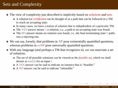
The view of complexity just described is implicitly based onsolutionsandsets.A solution (orcertificate) can be thought of as a path that can be followed in a TMto reach an accepting state.In many cases, we have a notion of solution that is indepdendent of a particular TM.TheYESanswer means∃ a solution, i.e., a path to an accepting state was found.TheNO answer means no solution was found, i.e., the final terminating state∀ pathswas a rejecting one.

We can say, loosely, that problems inNPpose existentially quantified questions,whereas problems incoNPpose universally quantified questions.

With any language (and perhaps a TM that recognizes it), we can associate a setof solutions.

The set of all possible solutions can be viewed as thefeasible set, which we shalldenote asfeas(l) for an inputl.A YESanswer can be said to indicate an instance that is “feasible.”A NO answer can be said to indicate “infeasible.”


Outline

1 Introduction




Turing Functions

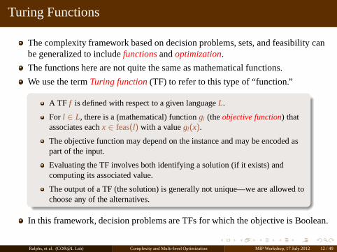
The complexity framework based on decision problems, sets,and feasibility canbe generalized to includefunctionsandoptimization.

The functions here are not quite the same as mathematical functions.

We use the termTuring function(TF) to refer to this type of “function.”

A TF f is defined with respect to a given languageL.

For l ∈ L, there is a (mathematical) functiongl (theobjective function) thatassociates eachx ∈ feas(l) with a valuegl(x).

The objective function may depend on the instance and may be encoded aspart of the input.

Evaluating the TF involves both identifying a solution (if it exists) andcomputing its associated value.

The output of a TF (the solution) is generally not unique—we are allowed tochoose any of the alternatives.

In this framework, decision problems are TFs for which the objective is Boolean.


Metric Turing Machines and Classes of Functions

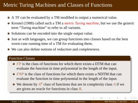
A TF can be evaluated by a TM modified to output a numerical value.

Krentel (1988) called such a TM ametric Turing machine, but we use the genericterm “Turing machine” to refer to all variants.

Solutions can be encoded into the single output value.

Just as with languages, we can group functions into classes based on the bestworst-case running time of a TM for evaluating them.

We can also define notions ofreductionandcompleteness.

Function Classes

FP is the class of functions for which there exists a DTM that canevaluate the function in time polynomial in the length of theinput.

FNP is the class of functions for which there exists a NDTM that canevaluate the function in time polynomial in the length of theinput.

We denote byAB class of functions that are in complexity classA if weare given an oracle for functions in classB.


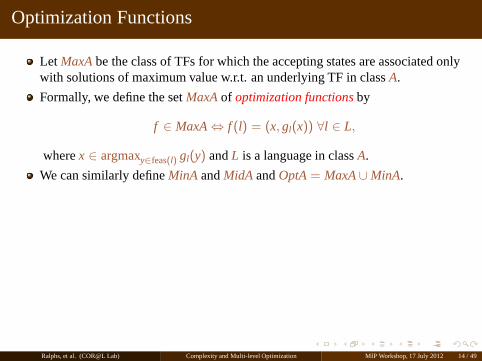
Optimization Functions

Let MaxAbe the class of TFs for which the accepting states are associated onlywith solutions of maximum value w.r.t. an underlying TF in classA.

Formally, we define the setMaxAof optimization functionsby

f ∈ MaxA⇔ f (l) = (x, gl(x)) ∀l ∈ L,

wherex ∈ argmaxy∈feas(l) gl(y) andL is a language in classA.

We can similarly defineMinA andMidA andOptA= MaxA∪ MinA.


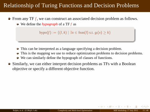
Relationship of Turing Functions and Decision Problems

From any TFf , we can construct an associated decision problem as follows.We define thehypographof a TFf as

hypo(f ) := {(l, k) | ∃x ∈ feas(l) s.t. gl(x) ≥ k}

This can be interpreted as a language specifying a decision problem.This is the mapping we use to reduce optimization problems todecision problems.We can similarly define the hypograph of classes of functions.

Similarly, we can either interpret decision problems as TFswith a Booleanobjective or specify a different objective function.


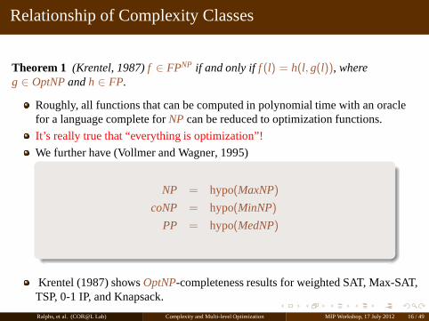
Relationship of Complexity Classes

Theorem 1 (Krentel, 1987)f ∈ FPNP if and only iff (l) = h(l, g(l)), whereg ∈ OptNPandh ∈ FP.

Roughly, all functions that can be computed in polynomial time with an oraclefor a language complete forNP can be reduced to optimization functions.

It’s really true that “everything is optimization”!

We further have (Vollmer and Wagner, 1995)

NP = hypo(MaxNP)

coNP = hypo(MinNP)

PP = hypo(MedNP)

Krentel (1987) showsOptNP-completeness results for weighted SAT, Max-SAT,TSP, 0-1 IP, and Knapsack.


Outline

1 Introduction




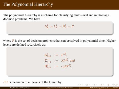
The Polynomial Hierarchy

The polynomial hierarchy is a scheme for classifying multi-level and multi-stagedecision problems. We have

∆p0 := Σp

0 := Πp0 := P,

whereP is the set of decision problems that can be solved in polynomial time. Higherlevels are defined recursively as:

∆pk+1 := PΣp

k ,

Σpk+1 := NPΣp

k , and

Πpk+1 := coNPΣp

k .

PH is the union of all levels of the hierarchy.


First Three Levels of the Hierarchy


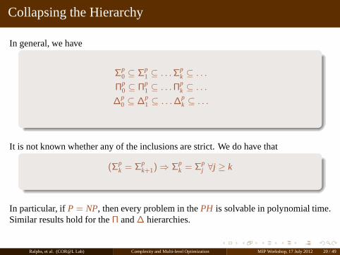
Collapsing the Hierarchy

In general, we have

Σp0 ⊆ Σp

1 ⊆ . . . Σpk ⊆ . . .

Πp0 ⊆ Πp

1 ⊆ . . . Πpk ⊆ . . .

∆p0 ⊆ ∆p

1 ⊆ . . .∆pk ⊆ . . .

It is not known whether any of the inclusions are strict. We dohave that

(Σpk = Σp

k+1) ⇒ Σpk = Σp

j ∀j ≥ k

In particular, ifP = NP, then every problem in thePH is solvable in polynomial time.Similar results hold for theΠ and∆ hierarchies.


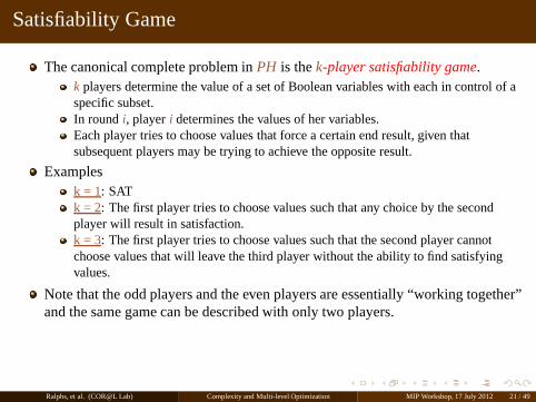
Satisfiability Game

The canonical complete problem inPH is thek-player satisfiability game.k players determine the value of a set of Boolean variables with each in control of aspecific subset.In roundi, playeri determines the values of her variables.Each player tries to choose values that force a certain end result, given thatsubsequent players may be trying to achieve the opposite result.

Examplesk = 1: SATk = 2: The first player tries to choose values such that any choice by the secondplayer will result in satisfaction.k = 3: The first player tries to choose values such that the second player cannotchoose values that will leave the third player without the ability to find satisfyingvalues.

Note that the odd players and the even players are essentially “working together”and the same game can be described with only two players.


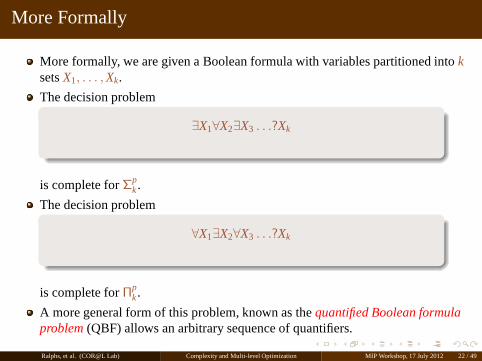
More Formally

More formally, we are given a Boolean formula with variablespartitioned intoksetsX1, . . . , Xk.

The decision problem

∃X1∀X2∃X3 . . .?Xk

is complete forΣpk.

The decision problem

∀X1∃X2∀X3 . . .?Xk

is complete forΠpk.

A more general form of this problem, known as thequantified Boolean formulaproblem(QBF) allows an arbitrary sequence of quantifiers.


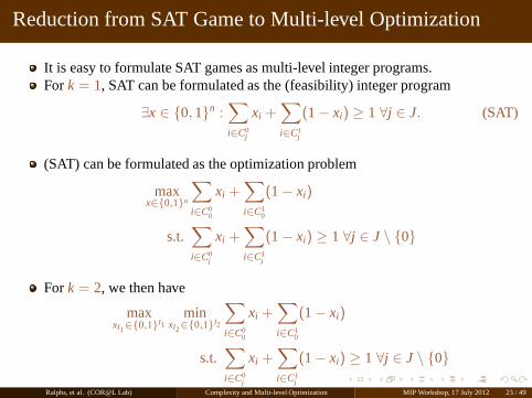
Reduction from SAT Game to Multi-level Optimization

It is easy to formulate SAT games as multi-level integer programs.Fork = 1, SAT can be formulated as the (feasibility) integer program

∃x ∈ {0, 1}n :∑

i∈C0j

xi +∑

i∈C1j

(1− xi) ≥ 1 ∀j ∈ J. (SAT)

(SAT) can be formulated as the optimization problem

maxx∈{0,1}n

∑

i∈C00

xi +∑

i∈C10

(1− xi)

s.t.∑

i∈C0j

xi +∑

i∈C1j

(1− xi) ≥ 1 ∀j ∈ J \ {0}

Fork = 2, we then have

maxxI1∈{0,1}I1

minxI2∈{0,1}I2

∑

i∈C00

xi +∑

i∈C10

(1− xi)

s.t.∑

i∈C0j

xi +∑

i∈C1j

(1− xi) ≥ 1 ∀j ∈ J \ {0}


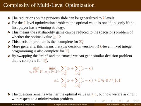
Complexity of Multi-Level Optimization

The reductions on the previous slide can be generalized tok levels.For thek-level optimization problem, the optimal value is one if andonly if thefirst player has a winning strategy.This means the satisfiability game can be reduced to the (decision) problem ofwhether the optimal value≥ 1?This decision problem is then complete forΣp

k.More generally, this means that (the decision version of)k-level mixed integerprogramming is also complete forΣp

k.By swapping the “min” and the “max,” we can get a similar decision problemthat is complete forΠp

k.

minxN1∈{0,1}N1

maxxN2∈{0,1}N2

∑

i∈C00

xi +∑

i∈C10

(1− xi)

s.t.∑

i∈C0j

xi +∑

i∈C1j

(1− xi) ≥ 1 ∀j ∈ J \ {0}

The question remains whether the optimal value is≥ 1, but now we are asking itwith respect to a minimization problem.Ralphs, et al. (COR@L Lab) Complexity and Multi-level Optimization MIP Workshop, 17 July 2012 24 / 49

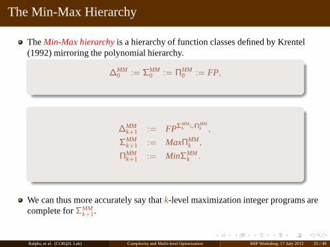
The Min-Max Hierarchy

TheMin-Max hierarchyis a hierarchy of function classes defined by Krentel(1992) mirroring the polynomial hierarchy.

∆MM0 := ΣMM

0 := ΠMM0 := FP,

∆MMk+1 := FPΣMM

k ∪ΠMMk ,

ΣMMk+1 := MaxΠMM

k ,

ΠMMk+1 := MinΣMM

k .

We can thus more accurately say thatk-level maximization integer programs arecomplete forΣMM

k+1.


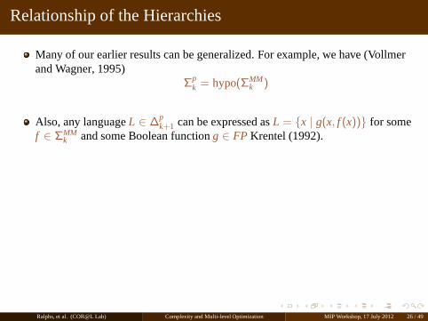
Relationship of the Hierarchies

Many of our earlier results can be generalized. For example,we have (Vollmerand Wagner, 1995)

Σpk = hypo(ΣMM

k )

Also, any languageL ∈ ∆pk+1 can be expressed asL = {x | g(x, f (x))} for some

f ∈ ΣMMk and some Boolean functiong ∈ FP Krentel (1992).


Alternating Turing Machines

An alternating Turing machine(ATM) can directly model the computationsrequired to solve multi-level optimization problems.In addition to accepting and rejecting states, these machines have two otherspecial classes of state.

The “∨” is accepting if there exists some configuration reachable in one stepthat is accepting and rejecting otherwise (∃).

The “∧” is accepting if all configurations reachable in one step areaccepting,and rejecting otherwise (∀).

Another way of thinking of this is that the final result is obtained by combiningthe states of all paths using the∨ and∧ operators.Such a machine can switch between existential and universalquantification andis thus capable of solving multi-level decision problems directly.ΣMM

k can be defined as languages recognizable on a machine with at mostkalternations on any given path.The canonical problem that can be solved by an ATM is the aforementionedQBF problem.Ralphs, et al. (COR@L Lab) Complexity and Multi-level Optimization MIP Workshop, 17 July 2012 27 / 49

Metric ATMs

A metric version of an ATM is one for which each branch is associated with a“max” or “min” operator.

The value output by the machine is calculated by combining the values in eachaccepting state with the “max” and “min” operators.

Metric ATMs can solve general multi-level optimization problems.

Subtrees of the execution tree encode the value functions oflower levelproblems.


Outline

1 Introduction




Separation Functions

Themembership problemfor a setSand a pointx is the decision problem ofdetermining whetherx ∈ S.An optimization version of this problem is

miny∈S

‖y− x‖ (SEP)

for norm‖ · ‖.We call (SEP) theseparation problemassociated withS.Theseparation functionassociated withf ∈ OptA, defined over a languageL, isan optimization function

f psep(x, l) = (y∗, ‖y∗ − x‖p),

wherey∗ ∈ argminy∈feas(l) ‖y− x‖p for l ∈ L.

For f ∈ OptAwith convex feasible set,f 2sep is closely related to the usual

separation problem.From the pointy∗, we can obtain a separating hyperplane.There are a number of alternative objective functions that can be employed.


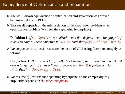
Equivalence of Optimization and Separation

The well-known equivalence of optimization and separationwas provenby Grötschel et al. (1988).

This result depends on the interpretation of the separationproblem as anoptimization problem (we need the separating hyperplane).

Definition 1 If f ∈ OptAis an optimization function defined over a languageL, fis said to have a linear objective if∃dl ∈ Rn such thatgl(x) = d⊤

l x ∀x ∈ feas(l).

We conjecture it is possible to state the result of GLS using functions, roughly asfollows.

Conjecture 1 (Grötschel et al., 1988) Letf be an optimization function definedover a languageL. If f has a linear objective andfeas(l) is polyhedral for alll ∈ L, thenf ∈ OptA⇔ f 2

sep∈ OptA.

We assumef 2sepreturns the separating hyperplane, so the complexity off

implicitly depends on thefacet complexity.


Outline

1 Introduction




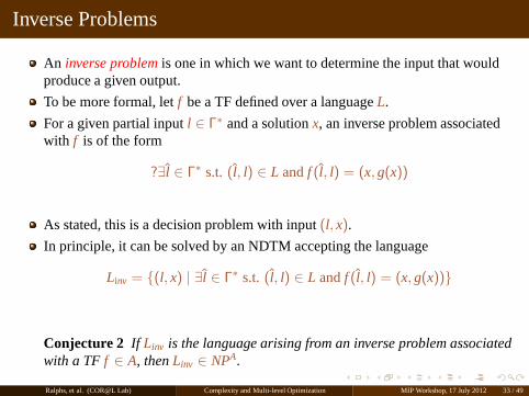
Inverse Problems

An inverse problemis one in which we want to determine the input that wouldproduce a given output.

To be more formal, letf be a TF defined over a languageL.

For a given partial inputl ∈ Γ∗ and a solutionx, an inverse problem associatedwith f is of the form

?∃l ∈ Γ∗ s.t. (l, l) ∈ L andf (l, l) = (x, g(x))

As stated, this is a decision problem with input(l, x).

In principle, it can be solved by an NDTM accepting the language

Linv = {(l, x) | ∃l ∈ Γ∗ s.t. (l, l) ∈ L andf (l, l) = (x, g(x))}

Conjecture 2 If Linv is the language arising from an inverse problem associatedwith a TFf ∈ A, thenLinv ∈ NPA.


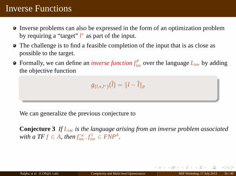
Inverse Functions

Inverse problems can also be expressed in the form of an optimization problemby requiring a “target”l∗ as part of the input.

The challenge is to find a feasible completion of the input that is as close aspossible to the target.

Formally, we can define aninverse functionf pinv over the languageLinv by adding

the objective function

g(l,x,l∗)(l) = ‖l − l‖p

We can generalize the previous conjecture to

Conjecture 3 If Linv is the language arising from an inverse problem associatedwith a TFf ∈ A, thenf∞inv , f 1

inv ∈ FNPA.


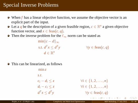
Special Inverse Problems

Whenf has a linear objective function, we assume the objective vector is anexplicit part of the input.Let aq be the description of a given feasible region,c ∈ Rn a given objectivefunction vector, andx ∈ feas(c, q).Then the inverse problem for theℓ∞ norm can be stated as

min‖c− d‖∞

s.t.dTx ≤ dTy ∀y ∈ feas(c, q)

d ∈ Rn

This can be linearized, as follows

minz

s.t.

ci − di ≤ z ∀i ∈ {1, 2, . . . , n}

di − ci ≤ z ∀i ∈ {1, 2, . . . , n}

dTx ≤ dTy ∀y ∈ feas(c, q)


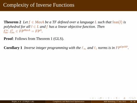
Complexity of Inverse Functions

Theorem 2 Let f ∈ MaxAbe a TF defined over a languageL such thatfeas(l) ispolyhedral for alll ∈ L andf has a linear objective function. Thenf∞inv , f 1

inv ∈ FPMaxA = FPA.

Proof: Follows from Theorem 1 (GLS).

Corollary 1 Inverse integer programming with theℓ∞ andℓ1 norms is inFPOptNP.


Outline

1 Introduction




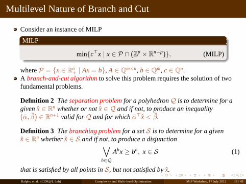
Multilevel Nature of Branch and Cut

Consider an instance of MILP

MILP

min{c⊤x | x ∈ P ∩ (Zp × Rn−p)}, (MILP)

whereP = {x ∈ Rn+ | Ax = b}, A ∈ Qm×n, b ∈ Qm, c ∈ Qn.

A branch-and-cut algorithmto solve this problem requires the solution of twofundamental problems.

Definition 2 Theseparation problemfor a polyhedronQ is to determine for agivenx ∈ Rn whether or notx ∈ Q and if not, to produce an inequality(α, β) ∈ Rn+1 valid forQ and for whichα⊤x < β.

Definition 3 Thebranching problemfor a setS is to determine for a givenx ∈ Rn whetherx ∈ S and if not, to produce a disjunction

∨

h∈Q

Ahx ≥ bh, x ∈ S (1)

that is satisfied by all points inS, but not satisfied byx.


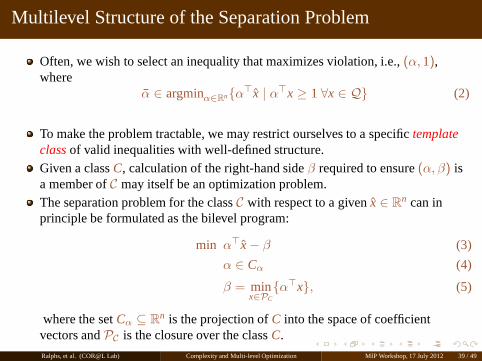
Multilevel Structure of the Separation Problem

Often, we wish to select an inequality that maximizes violation, i.e.,(α, 1),where

α ∈ argminα∈Rn{α⊤x | α⊤x ≥ 1 ∀x ∈ Q} (2)

To make the problem tractable, we may restrict ourselves to aspecifictemplateclassof valid inequalities with well-defined structure.Given a classC, calculation of the right-hand sideβ required to ensure(α, β) isa member ofC may itself be an optimization problem.The separation problem for the classC with respect to a givenx ∈ Rn can inprinciple be formulated as the bilevel program:

min α⊤x− β (3)

α ∈ Cα (4)

β = minx∈PC

{α⊤x}, (5)

where the setCα ⊆ Rn is the projection ofC into the space of coefficientvectors andPC is the closure over the classC.


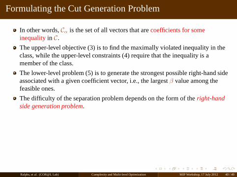
Formulating the Cut Generation Problem

In other words,Cα is the set of all vectors that arecoefficients for someinequalityin C.

The upper-level objective (3) is to find the maximally violated inequality in theclass, while the upper-level constraints (4) require that the inequality is amember of the class.

The lower-level problem (5) is to generate the strongest possible right-hand sideassociated with a given coefficient vector, i.e., the largest β value among thefeasible ones.

The difficulty of the separation problem depends on the form of the right-handside generation problem.


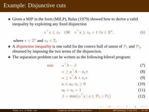
Example: Disjunctive cuts

Given a MIP in the form (MILP), Balas (1979) showed how to derive a validinequality by exploiting any fixed disjunction

π⊤x ≤ π0 OR π⊤x ≥ π0 + 1 ∀x ∈ Rn, (6)

whereπ ∈ Zn andπ0 ∈ Z.

A disjunctive inequalityis one valid for the convex hull of union ofP1 andP2,obtained by imposing the two terms of the disjunction.The separation problem can be written as the following bilevel program:

min α⊤x− β (7)

α ≥ u⊤A− uoπ (8)

α ≥ v⊤A + voπ (9)

u, v, u0, v0 ≥ 0 (10)

u0 + v0 = 1 (11)

β = min{α⊤x | x ∈ P1 ∪ P2} (12)


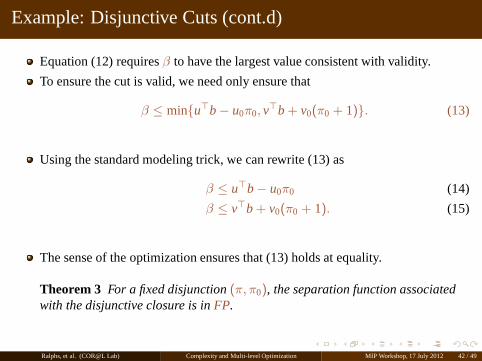
Example: Disjunctive Cuts (cont.d)

Equation (12) requiresβ to have the largest value consistent with validity.

To ensure the cut is valid, we need only ensure that

β ≤ min{u⊤b− u0π0, v⊤b + v0(π0 + 1)}. (13)

Using the standard modeling trick, we can rewrite (13) as

β ≤ u⊤b− u0π0 (14)

β ≤ v⊤b + v0(π0 + 1). (15)

The sense of the optimization ensures that (13) holds at equality.

Theorem 3 For a fixed disjunction(π, π0), the separation function associatedwith the disjunctive closure is inFP.


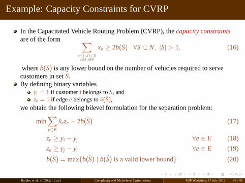
Example: Capacity Constraints for CVRP

In the Capacitated Vehicle Routing Problem (CVRP), thecapacity constraintsare of the form ∑

e={i,j}∈Ei∈S,j 6∈S

xe ≥ 2b(S) ∀S⊂ N, |S| > 1, (16)

whereb(S) is any lower bound on the number of vehicles required to servecustomers in setS.By defining binary variables

yi = 1 if customeri belongs toS, andze = 1 if edgee belongs toδ(S),

we obtain the following bilevel formulation for the separation problem:

min∑

e∈E

xeze − 2b(S) (17)

ze ≥ yi − yj ∀e∈ E (18)

ze ≥ yj − yi ∀e∈ E (19)

b(S) = max{b(S) | b(S) is a valid lower bound} (20)


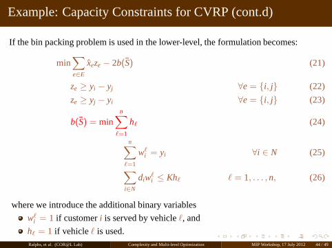
Example: Capacity Constraints for CVRP (cont.d)

If the bin packing problem is used in the lower-level, the formulation becomes:

min∑

e∈E

xeze − 2b(S) (21)

ze ≥ yi − yj ∀e = {i, j} (22)

ze ≥ yj − yi ∀e = {i, j} (23)

b(S) = minn∑

ℓ=1

hℓ (24)

n∑

ℓ=1

wℓi = yi ∀i ∈ N (25)

∑

i∈N

diwℓi ≤ Khℓ ℓ = 1, . . . , n, (26)

where we introduce the additional binary variables

wℓi = 1 if customeri is served by vehicleℓ, and

hℓ = 1 if vehicleℓ is used.Ralphs, et al. (COR@L Lab) Complexity and Multi-level Optimization MIP Workshop, 17 July 2012 44 / 49

Complexity of the Separation Function for GSECs

Theorem 4 The optimization function described by(21)–(26) is in the complexityclassΣMM

2 .

Proof: Reduction to 2-Quantified 1-in-3 SAT.


Multi-level Structure of the Branching Problem

A typical criteria for selecting a branching disjunction isto maximize the boundincrease resulting from imposing the disjunction.

The problem of selecting the disjunction whose imposition results in the largestbound improvement has a naturalbilevel structure.

The upper-level variables can be used to model thechoice of disjunction(we’ll seean example shortly).The lower-level problem models thebound computationafter the disjunction hasbeen imposed.

In strong branching, we are solving this problem essentially by enumeration.

The bilevel branching paradigm is to select the branching disjunction directly bysolving abilevel program.


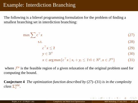
Example: Interdiction Branching

The following is a bilevel programming formulation for the problem of finding asmallest branching set in interdiction branching:

max∑

c⊤x (27)

s.t. (28)

c⊤x ≤ z (29)

y ∈ Bn (30)

x ∈ arg max{c⊤x | xi + yi ≤ 1∀i ∈ Na, x ∈ Fa} (31)

whereFa is the feasible region of a given relaxation of the original problem used forcomputing the bound.

Conjecture 4 The optimization function described by(27)–(31) is in the complexityclassΣMM

2 .


Further Generalizations and Conclusions

We can generate separation and branching functions of any level in thecomplexity hierarhcy by “looking ahead” multiple levels.

The separation functions for closures of rank> 1 are also likely in higher levelsof the hierarchy.

The framework presented here seems to be promising in terms of analyzing thecomplexity of these and related multi-level optimization problems.

This is a first stab at a general framework, but I’m sure it could use tweaking.

If you have thoughts, feel free to talk to me.


References I

Balas, E. 1979. Disjunctive programming.Annals of Discrete Mathematics5, 3–51.

Garey, M. and D. Johnson 1979.Computers and Intractability: A Guide to the Thoeryof NP-Completeness. W.H. Freeman and Company.

Grötschel, M., L. Lovász, and A. Schrijver 1988.Geometric Algorithms andCombinatorial Optimization. Springer-Verlag, New York.

Krentel, M. 1987.The Complexity of Optimization Problems. Ph.D. thesis, CornellUniversity.

— 1988. The complexity of optimization problems.Journal of Computer and SystemSciences36, 490–509.

— 1992. Generalizations of optp to the polynomial hierarchy. Theoretical ComputerScience97, 183–198.

Vollmer, H. and K. Wagner 1995. Complexity classes of optimization functions.Information and Computation120, 198–219.


complexity and multi-level optimizationted/files/talks/mip12.pdf · motivation the framework...

Documents