complexfinslermetrics by marco abate and giorgio patrizio · by marco abate and giorgio patrizio...

arX

iv:m

ath/

9310

201v

1 [

mat

h.C

V]

31

Oct

199

3

Complex Finsler metrics

by Marco Abate and Giorgio Patrizio

Seconda Universita di Roma00133 Roma, Italy

September 1993

Dedicated to Prof. S. Kobayashi

0. Introduction

A complex Finsler metric is an upper semicontinuous function F :T 1,0M → R+ defined on

the holomorphic tangent bundle of a complex Finsler manifold M , with the property thatF (p; ζv) = |ζ|F (p; v) for any (p; v) ∈ T 1,0M and ζ ∈ C.

Complex Finsler metrics do occur naturally in function theory of several variables.The Kobayashi metric introduced in 1967 ([K1]) and its companion the Caratheodorymetric are remarkable examples which have become standard tools for anybody workingin complex analysis; we refer the reader to [K2, 4], [L], [A] and [JP] to get an idea of theamazing developments in this area achieved in the past 25 years.

In general, the Kobayashi metric is not at all regular; it may even not be continuous.But in 1981 Lempert [Le] proved that the Kobayashi metric of a bounded strongly convexdomain D in C

n is smooth (outside the zero section of T 1,0D), thus allowing in principlethe use of differential geometric techniques in the study of function theory over stronglyconvex domains (see also Pang [P2] for other examples of domains with smooth Kobayashimetric).

We started dealing with this kind of problems in [AP1]. In particular, [AP2] wasdevoted to the search of differential geometric conditions ensuring the existence in a com-plex Finsler manifold of a foliation in holomorphic disks like the one found by Lempertin strongly convex domains, where the disks were isometric embeddings of the unit disk∆ ⊂ C endowed with the Poincare metric. And indeed (see also [AP3]) we found neces-sary and sufficient conditions (see also Pang [P1] for closely related results). In that case,because the nature of the problem required the solution of certain P.D.E.’s, the conditionswere mainly expressed in local coordinates somewhat hiding their geometric meaning.

The aim of this paper is to present an introduction to complex Finsler geometry in away suitable to deal with global questions. Roughly speaking, the idea is to isometricallyembed a complex Finsler manifold into a hermitian vector bundle, and then apply standardhermitian differential geometry techniques, in the spirit of [K3]. Here we provide just acoarse outline of the procedure. Let M be the complement of the zero section in T 1,0M .We assume that the complex Finsler metric F is smooth on M , and that F is stronglypseudoconvex, that is that the Levi form of G = F 2 is positive definite. Now let V ⊂ T 1,0Mbe the vertical bundle, that is the kernel of the differential of the canonical projectionπ:T 1,0M → M . Using the Levi form of G, it is easy to define a hermitian metric on V;moreover, there exists a canonical section ι of V giving an isometric embedding of M into V

http://arxiv.org/abs/math/9310201v1

2 Marco Abate and Giorgio Patrizio

— that is for any v ∈ M the norm of ι(v) with respect to the given hermitian metric on Vis equal to F (v). Let D be the Chern connection on V associated to the metric, and denoteby H the kernel of the bundle map X 7→ ∇Xι. Then it turns out that H is a horizontalbundle, that is T 1,0M = H⊕ V; furthermore, there is a canonically defined global bundleisomorphism Θ:V → H. Using Θ, we can transfer both the metric and the connection onH,obtaining a canonical hermitian structure on T 1,0M , and the associated Chern connectionpreserves the splitting. Finally, the horizontal radial vector field χ = Θ ι is a canonicalisometric embedding of M into H. Then our idea is that the complex Finsler geometryof M should be described by using the differential geometry of the Chern connection Drestricted to H, using χ as a means of transfering informations from the tangent bundleto the horizontal bundle and back. For instance, the Kahler condition introduced in [AP2]becomes the vanishing of a suitable contraction of the horizontal part of the torsion of D(here we say that the metric is weakly Kahler); and the necessary and sufficient conditionfor the existence of complex geodesic curves (see [AP2, 3]) are expressed by constantholomorphic curvature and a symmetry property of the horizontal part of the curvatureof D; cf. Lemma 8.3.

This approach is in the spirit of the one developed by E. Cartan [C] for real Finslermetrics; see [Ru1], [M], [Ch], [BC], [Be] and the forthcoming monograph [AP4] for anaccount in modern language. On the other hand, to our surprise we were unable to findin the literature a comparable approach in the complex case. Rund, in [Ru2], describedthe Chern connection on the horizontal bundle, but only in local coordinates. Fukuiin [Fu] studied the Cartan connection on a complex Finsler manifold, which is in generaldifferent from the Chern connection (see [AP4] for a comparison). Faran [F] studied thelocal equivalence problem, without dealing with global questions. Only Kobayashi [K3]explicitely used the Chern connection, but he seemed unaware of the relevance of thehorizontal component. It should be mentioned that we choose to work on M instead ofthe projectivized tangent bundle mainly for keeping more transparent the relationshipsbetween global objects and local computations (which are often simplified by consistentlyusing the homogeneity of the function G and its derivatives). However the two approachare completely equivalent. In fact, the role of the canonical sections ι and χ in our contextis analogous to the role of the tautological line bundle in [K3]. We hope that our work willclarify the subject of complex Finsler geometry, opening the way to new research in thefield.

The content of this paper is the following. In sections 1 and 2 we describe in detailthe construction outlined above of the Chern-Finsler connection. In sections 3 and 4 wedefine the (2,0)-torsion, the (1,1)-torsion, the curvature of the Chern-Finsler connectionon the horizontal bundle, we derive the Bianchi identities and we discuss Kahler Finslermetrics. In section 5 we introduce the notion of holomorphic curvature.

In sections 6 and 7 we derive the first and second variation formulas for a stronglypseudoconvex Kahler Finsler metric, giving a good example of global computations madeusing the tools introduced before. As a corollary, we prove the local existence and unique-ness of geodesics for a strongly pseudoconvex weakly Kahler metric, without assuming thestrong convexity of the metric.

Finally, in section 8 we deal with strongly pseudoconvex Finsler metrics of constant

Complex Finsler metrics 3

holomorphic curvature, providing a first step toward their classification. As a consequenceof results of this section and of [AP2] we get for example the following:

Theorem 0.1: Let F :T 1,0M → R+ be a complete strongly pseudoconvex Finsler metric

on a simply connected complex manifold M . Assume that

(i) F is Kahler;(ii) F has constant holomorphic curvature −4;(iii) R(H,K, χ, χ) = R(χ,K,H, χ) for all H, K ∈ H, where R is the curvature operatorof the Chern connection;(iv) the indicatrices IF (p) = v ∈ T 1,0

p M | F (v) < 1 of F are strongly convex forall p ∈M .

Then the exponential map expp:T1,0p M → M is a homeomorphism, and a smooth diffeo-

morphism outside the origin, for any p ∈ M . Furthermore, a suitable reparametrizationof expp induces a foliation of M by isometric totally geodesic holomorphic embeddings ofthe unit disk ∆ ⊂ C endowed with the Poincare metric. In particular, F is the Kobayashimetric of M .

A version of this result also holds when the holomorphic curvature is identically zero;the precise statement can be found in Theorem 8.10

1. Definitions and preliminaries

LetM be a complex manifold of complex dimension n. We shall denote by T 1,0M the holo-morphic tangent bundle ofM , and by M the complement in T 1,0M of the zero section. Thereal tangent bundle of M will be denoted by TRM , and we set as usual TCM = TRM ⊗C.

A complex Finsler metric F onM is an upper semicontinuous function F :T 1,0M → R+

satisfying

(i) G = F 2 is smooth on M ;(ii) F (p; v) > 0 for all p ∈M and v ∈ Mp;(iii) F

(

p; ζv)

= |ζ|F (p; v) for all p ∈M , v ∈ T 1,0p M and ζ ∈ C.

We shall sistematically denote by G the function G = F 2. Note that it is important toask for the smoothness of G only on M : in fact, it is easy to see that G is smooth on thewhole of T 1,0M iff F is the norm associated to a hermitian metric. In this case, we shallsay that F comes from a hermitian metric.

To start, we need a few notations and general formulas. In local coordinates, a vectorv ∈ T 1,0

p M is written as

v = vα∂

∂zα

∣

∣

∣

∣

p

,

where we adopt the Einstein convention. In particular, the function G is locally expressedin terms of the coordinates z1, . . . , zn, v1, . . . , vn. We shall denote by indices like α, βand so on the derivatives with respect to the v-coordinates; for instance,

Gαβ =∂2G

∂vα∂vβ.


On the other hand, the derivatives with respect to the z-coordinates will be denoted byindices after a semicolon; for instance,

G;µν =∂2G

∂zµ∂zνor Gα;ν =

∂2G

∂zν∂vα.

For our aims, we ought to focus on a smaller class of Finsler metrics. A complexFinsler metric F will be said strongly pseudoconvex if

(iv) the Levi matrix (Gαβ) is positive definite on M .

This is equivalent to requiring that all the F -indicatrices

IF (p) = v ∈ T 1,0p M | F (v) < 1

are strongly pseudoconvexes. As we shall see in section 2, this hypothesis will allow us todefine a hermitian metric on a suitable vector bundle.

The main (actually, almost the unique) property of the function G is its (1,1)-hom-ogeneity: we have

G(p; ζv) = ζζ G(p; v) (1.1)

for all (p; v) ∈ T 1,0M and ζ ∈ C. We now collect a number of formulas we shall use later

on which are consequences of (1.1). First of all, differentiating with respect to vα and vβ

we getGα(p; ζv) = ζGα(p; v),

Gαβ(p; ζv) = Gαβ(p; v),

Gαβ(p; ζv) = (ζ/ζ)Gαβ(p; v).

(1.2)

Thus differentiating with respect to ζ or ζ and then setting ζ = 1 we get

Gαβ vβ = Gα, Gαβ v

β = 0, (1.3)

andGαβγ v

γ = −Gαβ , Gαβγ vγ = Gαβ , Gαβγ vγ = 0, (1.4)

where everything is evaluated at (p; v).On the other hand, differentiating directly (1.1) with respect to ζ or ζ and putting

eventually ζ = 1 we get

Gα vα = G, Gαβ v

αvβ = 0, Gαβ vαvβ = G. (1.5)

It is clear that we may get other formulas applying any differential operator acting onlyon the z-coordinates, or just by conjugation. For instance, we get

Gα;µ vα = G;µ, (1.6)

and so on.


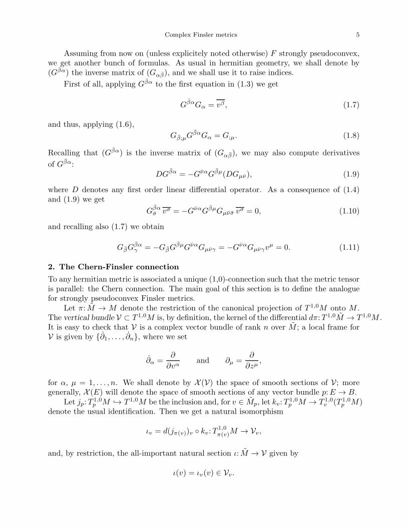
Assuming from now on (unless explicitely noted otherwise) F strongly pseudoconvex,we get another bunch of formulas. As usual in hermitian geometry, we shall denote by(Gβα) the inverse matrix of (Gαβ), and we shall use it to raise indices.

First of all, applying Gβα to the first equation in (1.3) we get

GβαGα = vβ , (1.7)

and thus, applying (1.6),

Gβ;µGβαGα = G;µ. (1.8)

Recalling that (Gβα) is the inverse matrix of (Gαβ), we may also compute derivatives

of Gβα:DGβα = −GναGβµ(DGµν), (1.9)

where D denotes any first order linear differential operator. As a consequence of (1.4)and (1.9) we get

Gβασ vσ = −GναGβµGµνσ vσ = 0, (1.10)

and recalling also (1.7) we obtain

GβGβαγ = −GβG

βµGναGµνγ = −GναGµνγvµ = 0. (1.11)

2. The Chern-Finsler connection

To any hermitian metric is associated a unique (1,0)-connection such that the metric tensoris parallel: the Chern connection. The main goal of this section is to define the analoguefor strongly pseudoconvex Finsler metrics.

Let π: M → M denote the restriction of the canonical projection of T 1,0M onto M .The vertical bundle V ⊂ T 1,0M is, by definition, the kernel of the differential dπ:T 1,0M → T 1,0M .It is easy to check that V is a complex vector bundle of rank n over M ; a local frame forV is given by ∂1, . . . , ∂n, where we set

∂α =∂

∂vαand ∂µ =

∂

∂zµ,

for α, µ = 1, . . . , n. We shall denote by X (V) the space of smooth sections of V; moregenerally, X (E) will denote the space of smooth sections of any vector bundle p:E → B.

Let jp:T1,0p M → T 1,0M be the inclusion and, for v ∈ Mp, let kv:T

1,0p M → T 1,0

v (T 1,0p M)

denote the usual identification. Then we get a natural isomorphism

ιv = d(jπ(v))v kv:T1,0π(v)M → Vv,

and, by restriction, the all-important natural section ι: M → V given by

ι(v) = ιv(v) ∈ Vv.


In local coordinates,

ιv

(

∂

∂zα

∣

∣

∣

∣

π(v)

)

= ∂α|v;

in particular, if v = vα(∂/∂zα) then

ι(v) = vα∂α|v.

ι is called the radial vertical vector field.The first observation is that a strongly pseudoconvex Finsler metric F defines a hermi-

tian metric on the vertical bundle V. Indeed, if v ∈ M andW1,W2 ∈ Vv, withWj =Wαj ∂α,

we set〈W1,W2〉v = Gαβ(v)W

α1 W

β2 .

Being F strongly pseudoconvex, 〈 , 〉 is a hermitian metric. Note that the third equationin (1.5) says that

G = 〈ι, ι〉;

so ι is an isometric embedding of M into V.Following Kobayashi [K3], we now consider the Chern connectionD on the vector bun-

dle V: it is the unique (1,0)-connection on V such that the hermitian structure previouslydefined is parallel. In other words, D:X (V) → X (T ∗

CM ⊗ V) is such that

X〈V,W 〉 = 〈∇XV,W 〉+ 〈V,∇XW 〉,

for any X ∈ T 1,0M and V , W ∈ X (V).In local coordinates, the connection matrix (ωα

β ) is given by

ωαβ = Gτα∂Gβτ = Γα

β;µ dzµ + Γα

βγ dvγ ,

whereΓαβγ = GταGβτγ and Γα

β;µ = GταGβτ ;µ.

This is only part of the connection we are looking for: our next goal is to canonicallyextend D to a (1,0)-connection on T 1,0M . Let us consider the bundle map Λ:T 1,0M → Vdefined by

Λ(X) = ∇X ι,

and setH = kerΛ ⊂ T 1,0M . We claim thatH is a horizontal bundle, that is T 1,0M = H⊕V.Indeed, in local coordinates

Λ(X) = [Xα + ωαβ (X)vβ]∂α,

where X = Xµ∂µ + Xα∂α. Then a local frame for H is given by δ1, . . . , δn, where

δµ = ∂µ − Γαβ;µv

β ∂α


— note that Γαβγv

β ≡ 0 — and the claim is proved.It is not difficult to check (see [AP4] for a coordinate-free proof) that setting

Θ(∂α) = δα

for α = 1, . . . , n we get a well-defined global bundle isomorphism Θ:V → H; then we candefine a (1,0)-connnection D on H just by setting

∇XH = Θ[

∇X(Θ−1H)]

for any X ∈ TCM and H ∈ X (H). By linearity, this yields a (1,0)-connection on T 1,0M ,still denoted by D: the Chern-Finsler connection.

Using the bundle isomorphism Θ:V → H we can also transfer the hermitian struc-ture 〈 , 〉 on H just by setting

∀H,K ∈ Hv 〈H,K〉v = 〈Θ−1(H),Θ−1(K)〉v,

and then we can define a hermitian structure on T 1,0M by requiring H be orthogonalto V. It is easy to check then that D is the Chern connection associated to this hermitianstructure, that is

X〈Y, Z〉 = 〈∇XY, Z〉+ 〈Y,∇XZ〉

for any X ∈ T 1,0M and Y , Z ∈ X (T 1,0M).¿From now on we shall work only with the frame δµ, ∂α and its dual co-frame

dzµ, ψα given byψα = dvα + Γα

;µ dzµ = dvα +GταGτ ;µ dz

µ,

where we have setΓα;µ = Γα

β;µvβ = GταGτ ;µ.

Writingωαβ = Γα

β;µ dzµ + Γα

βγψγ,

we getΓαβγ = GταGβτγ = Γα

γβ ,

Γαβ;µ = Gταδµ(Gβτ ) = Gτα(Gβτ ;µ −GβτγΓ

γµ).

(2.1)

Note thatΓαβ;µ = ∂β(Γ

α;µ) and Γα

;µ = Γαβ;µv

β ; (2.2)

in particular, this is exactly the connection introduced by Rund [Ru2].So we have described a canonical splitting of the holomorphic tangent bundle of M

in a vertical and a horizontal bundle, and defined a canonical connection on it, preservingthis splitting. In the following subsections we shall begin the study of this connection,introducing torsions and curvatures; here we first describe a few properties of the splitting.

First of all, the next lemma shows that the local frames δ1, . . . , δn enjoy some niceand convenient properties:


Lemma 2.1: Let D be the Chern-Finsler connection associated to a strongly pseudocon-vex Finsler metric F , and let δ1, . . . , δn be the corresponding local horizontal frame.Then

(i) [δµ, δν ] = 0 for all 1 ≤ µ, ν ≤ n;

(ii) [δµ, ∂α] = Γσα;µ∂σ for all 1 ≤ α, µ ≤ n;

(iii) δµ(G) = δµ(G) = 0 for all 1 ≤ µ ≤ n;(iv) δµ(Gα) = 0 for all 1 ≤ α, µ ≤ n.

Proof : (i) If suffices to compute. First of all,

[δµ, δν ] = (Γα;µν − Γα

;νµ + Γασ;νΓ

σ;µ − Γα

σ;µΓσ;ν)∂α,

where Γα;µν = ∂ν(Γ

α;µ) and so on. Now,

Γα;µν = Gτα(Gτ ;µν −Gστ ;νΓ

σ;µ),

Γα;νµ = Gτα(Gτ ;νµ −Gστ ;µΓ

σ;ν),

Γασ;νΓ

σ;µ = Gτα(Gστ ;νΓ

σ;µ −GστρΓ

ρ;νΓ

σ;µ),

Γασ;µΓ

σ;ν = Gτα(Gστ ;µΓ

σ;ν −GστρΓ

ρ;µΓ

σ;ν),

and the assertion follows. Note that we have actually proved that

δν(Γα;µ) = δµ(Γ

α;ν). (2.3)

(ii) Indeed,

[δµ, ∂α] = [∂µ − Γσ;µ∂σ, ∂α] = ∂α(Γ

σ;µ)∂σ = Γσ

α;µ∂σ.

(iii) In fact, using (1.8) we get

δµ(G) = G;µ − Γσ;µGσ = G;µ −GτσGτ ;µGσ = G;µ −G;µ = 0.

(iv) Finally,δµ(Gα) = Gα;µ − Γτ

;µGατ = Gα;µ −Gα;µ = 0,

where Γτ;µ = Γτ

;µ.

The philosophical idea behind our work is that to study the geometry of a complexFinsler metric one should transfer everything (or most of it) in the horizontal bundle, andthen apply the usual techniques of hermitian geometry there. We shall better substantiatethis idea later, for instance in sections 6 and 7 discussing variation formulas; here we beginto show how to lift objects (e.g., vector fields) from the tangent bundle up to H.

The main tool is provided by the horizontal analogues of the isomorphisms ιv. Ifv ∈ M , we set

χv = Θv ιv:Tπ(v)M → Hv.

The horizontal radial vector field χ ∈ X (H) is then defined by

χ = Θ ι;


in local coordinates, if v = vα(∂/∂zα)|p we have

χ(v) = vαδα|v.

Using the isomorphisms χv we can induce an embedding of M into H which respectsthe Lie algebra structure. To be precise, a vector field ξ ∈ X (T 1,0M) may be lifted in twodifferent ways to vector fields in T 1,0M : via the horizontal lift

ξH(v) = χv

(

ξ(

π(v))

)

,

and via the vertical liftξV (v) = ιv

(

ξ(

π(v))

)

.

A consequence of Lemma 2.1 is that the horizontal lift is a Lie algebra homomorphism:

Proposition 2.2: Let D be the Chern-Finsler connection associated to a strongly pseu-doconvex Finsler metric F on a complex manifold M . Then:

(i) [X (H),X (H)] ⊂ X (H) and [X (V),X (V)] ⊂ X (V);(ii) if ξ1, ξ2 ∈ X (M) then [ξH1 , ξ

H2 ] = [ξ1, ξ2]

H , [ξV1 , ξV2 ] = 0 and [ξH1 , ξ

V2 ] ∈ X (V).

Proof : (i) Take H1, H2 ∈ X (H). Locally, Hj = Hµj δµ; hence

[H1, H2] =(

Hν1 δν(H

µ2 )−Hν

2 δν(Hµ1 ))

δµ (2.4)

(where we used Lemma 2.1) is horizontal. Analogously, if V1, V2 ∈ X (V) with Vj = V αj ∂α,

we get[V1, V2] =

(

V β1 ∂β(V

α2 )− V β

2 ∂β(Vα1 ))

∂α, (2.5)

which is vertical.(ii) Locally, ξj = ξµj (∂/∂z

µ) and ξHj = (ξµj π)δµ; so (2.4) yields

[ξH1 , ξH2 ] =

(

(ξν1 π)δν(ξµ2 π)− (ξν2 π)δν(ξ

µ1 π)

)

δµ.

Now δν(ξµj π) = (∂ξµj /∂z

ν) π; therefore

[ξH1 , ξH2 ] =

[(

ξν1∂ξµ2∂zν

− ξν2∂ξµ1∂zν

)

π

]

δµ = [ξ1, ξ2]H .

On the other hand, ξVj = (ξαj π)∂α and ∂β(ξαj π) = 0 yield

[ξV1 , ξV2 ] = 0.

Finally,

[ξH1 , ξV2 ] =

[(

ξµ1∂ξα2∂zµ

)

π +(

(ξµ1 ξβ2 ) π

)

Γαβ;µ

]

∂α,

again by Lemma 2.1.

Note that, as a consequence of (ii), the obvious map of X (V) into X (H) induced bythe complex horizontal map Θ:V → X is not an isomorphism of Lie algebras; it suffices toremark that Θ(ξV ) = ξH for all ξ ∈ X (M).


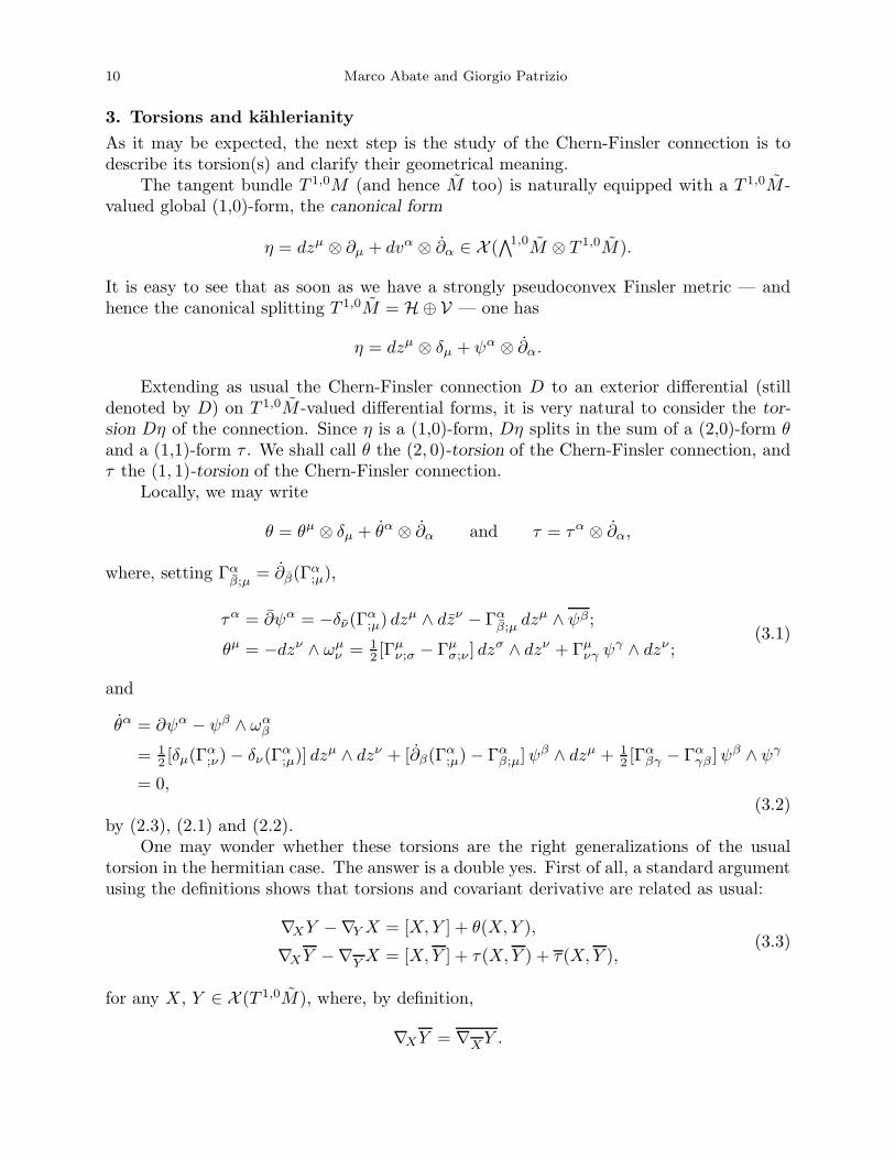
3. Torsions and kahlerianity

As it may be expected, the next step is the study of the Chern-Finsler connection is todescribe its torsion(s) and clarify their geometrical meaning.

The tangent bundle T 1,0M (and hence M too) is naturally equipped with a T 1,0M -valued global (1,0)-form, the canonical form

η = dzµ ⊗ ∂µ + dvα ⊗ ∂α ∈ X (∧1,0

M ⊗ T 1,0M).

It is easy to see that as soon as we have a strongly pseudoconvex Finsler metric — andhence the canonical splitting T 1,0M = H⊕ V — one has

η = dzµ ⊗ δµ + ψα ⊗ ∂α.

Extending as usual the Chern-Finsler connection D to an exterior differential (stilldenoted by D) on T 1,0M -valued differential forms, it is very natural to consider the tor-sion Dη of the connection. Since η is a (1,0)-form, Dη splits in the sum of a (2,0)-form θand a (1,1)-form τ . We shall call θ the (2, 0)-torsion of the Chern-Finsler connection, andτ the (1, 1)-torsion of the Chern-Finsler connection.

Locally, we may write

θ = θµ ⊗ δµ + θα ⊗ ∂α and τ = τα ⊗ ∂α,

where, setting Γαβ;µ

= ∂β(Γα;µ),

τα = ∂ψα = −δν(Γα;µ) dz

µ ∧ dzν − Γαβ;µ dz

µ ∧ ψβ;

θµ = −dzν ∧ ωµν = 1

2 [Γµν;σ − Γµ

σ;ν ] dzσ ∧ dzν + Γµ

νγ ψγ ∧ dzν ;

(3.1)

and

θα = ∂ψα − ψβ ∧ ωαβ

= 12 [δµ(Γ

α;ν)− δν(Γ

α;µ)] dz

µ ∧ dzν + [∂β(Γα;µ)− Γα

β;µ]ψβ ∧ dzµ + 1

2 [Γαβγ − Γα

γβ ]ψβ ∧ ψγ

= 0,(3.2)

by (2.3), (2.1) and (2.2).One may wonder whether these torsions are the right generalizations of the usual

torsion in the hermitian case. The answer is a double yes. First of all, a standard argumentusing the definitions shows that torsions and covariant derivative are related as usual:

∇XY −∇YX = [X, Y ] + θ(X, Y ),

∇XY −∇YX = [X, Y ] + τ(X, Y ) + τ(X, Y ),(3.3)

for any X , Y ∈ X (T 1,0M), where, by definition,

∇XY = ∇XY .


Furthermore, the vanishing of (part of) the (2,0)-torsion can be again interpreted asa Kahler condition — but with some care, because θ is composed by a horizontal part anda mixed part. To be precise, we shall say that a differential form γ on M is horizontal ifit vanishes contracted with any V ∈ X (V). The decomposition T 1,0M = H⊕ V induces aprojection p∗H of the differential forms onto the horizontal forms; the horizontal part of aform γ is then p∗H(γ).

There is a corresponding projection on the vertical forms, of course, but we shall notneed it now because the vertical part of both torsions θ and τ is zero. For this reason, theform θ − p∗H(θ) will be called the mixed part of θ. In local coordinates,

p∗H(θ) = (Γσν;µ dz

µ ∧ dzν)⊗ δσ and θ − p∗H(θ) = (Γσνγ ψ

γ ∧ dzν)⊗ δσ.

The next proposition discusses the meaning of the vanishing of the (2,0)-torsion θ or ofone of its parts.

Proposition 3.1: Let F be a strongly pseudoconvex Finsler metric on a complex mani-fold M . Then:

(i) the mixed part of the (2, 0)-torsion vanishes iff F comes from a hermitian metric;(ii) θ vanishes iff F comes from a hermitian Kahler metric.

Proof : (i) The mixed part of the torsion vanishes iff Gβµγ = 0 for all β, µ and γ. Conju-

gating, this is equivalent to having ∂γ(Gβµ) = ∂γ(Gβµ) = 0, that is Gβµ(v) depends onlyon π(v) — and this happens iff F comes from a hermitian metric.

(ii) It follows from (i) and the fact that when F comes from a hermitian metricg = (gαβ) one has

Γαβ;µ = gτα

∂gβτ∂zµ

.

For this reason we say that a strongly pseudoconvex Finsler metric F is stronglyKahler if the horizontal part of the (2,0)-torsion vanishes, that is iff

∀H,K ∈ H θ(H,K) = 0.

This is exactly the notion of kahlerianity introduced by Rund [Ru2]. However, as we shallsee later on (see sections 6 and 7), studying the geometry of a strongly pseudoconvexFinsler metric it turns out that this assumption is too strong and not quite natural. So itis appropriate to introduce two more notions of kahlerianity. We shall say that F is Kahlerif

∀H ∈ H θ(H,χ) = 0,

and that F is weakly Kahler if

∀H ∈ H 〈θ(H,χ), χ〉 = 0.


In local coordinates, F is strongly Kahler iff

Γαµ;ν = Γα

ν;µ;

it is Kahler iffΓαµ;νv

µ = Γαν;µv

µ;

it is weakly Kahler iffGα[Γ

αµ;ν − Γα

ν;µ]vµ = 0,

that is iff

0 = [Gµ;ν −Gν;µ +GνσΓσ;µ]v

µ = [Gµτ ;ν −Gντ ;µ +GνστΓσ;µ]v

µvτ .

In particular, if F comes from a hermitian metric then these three conditions are allequivalent to the usual Kahler condition, because Gνστ ≡ 0 for a Finsler metric comingfrom a hermitian metric.

There are other characterizations of strongly Kahler Finsler metrics. To F we mayassociate the fundamental form

Φ = iGαβ dzα ∧ dzβ ,

which is a well-defined real (1,1)-form on M . Then the strong Kahler condition is equivalentto the vanishing of the horizontal part of dΦ. To express it more clearly, set

dH = p∗H d, ∂H = p∗H ∂ and ∂H = p∗H ∂,

so that again dH = ∂H + ∂H .

Theorem 3.2: Let F be a strongly pseudoconvex Finsler metric on a complex manifoldM .Then the following assertions are equivalent:

(i) F is a strongly Kahler Finsler metric;(ii) ∇HK −∇KH = [H,K] for all H, K ∈ X (H);(iii) dHΦ = 0;(iv) ∂HΦ = 0;(v) for any p0 ∈ M there is a neighbourhood U of p0 in M and a real-valued functionφ ∈ C∞

(

π−1(U))

such that Φ = i∂H ∂Hφ on π−1(U).

Proof : (i) ⇐⇒ (ii) follows from (3.3).(iii) ⇐⇒ (iv) holds simply because Φ is a real (1,1)-form.(iv) ⇐⇒ (i). Indeed, (2.1) yields

∂Φ(X, Y, Z) = i〈θ(X, Y ), Z〉

for all X , Y , Z ∈ T 1,0M ; hence ∂HΦ vanishes iff p∗H θ vanishes, that is iff F is stronglyKahler.

(v) =⇒ (iv) follows from Lemma 2.1.(i).


(iii) =⇒ (v). Let γ be any horizontal form. In local coordinates, defined on a coordi-nate neighbourhood of the form π−1(U), one has

γ|(p;v) = γAB(p; v) dzA ∧ dzB ,

for suitable multi-indices A and B. On U we may then consider the family of forms

γv|p = γAB(p; v) dzA ∧ dzB ,

where here dzj is the dual frame of ∂/∂zj; in other words, we are considering thev-coordinates just as parameters.

The gist is that the following formula holds:

(dHγ)v = d(γv).

Then we may now apply the Dolbeault and Serre theorems (with parameters) to Φv

in a possibly smaller neighbourhood of p0 — still denoted by U — to get a functionφv ∈ C∞(U,R) depending smoothly on v such that Φv = i∂∂φv. Then setting

φ(p; v) = φv(p)

we get Φ = i∂H ∂Hφ, as required.

¿From this point of view, a strongly pseudoconvex Finsler metric is Kahler iff

dHΦ(·, χ, ·) ≡ 0,

and it is weakly Kahler iffdHΦ(·, χ, χ) ≡ 0.

We end this section pointing out that also the vanishing of the (1,1)-torsion τ has anice geometric meaning:

Proposition 3.3: The (1, 1)-torsion τ vanishes iff the frame δµ, ∂α is holomorhic.

Proof : Indeed the frame δµ, ∂α is holomorphic iff its dual coframe dzµ, ψα is, whichhappens iff the forms ψα are holomorphic, that is iff τα = ∂ψα = 0 for α = 1, . . . , n.

4. The curvature tensor

The curvature tensor R:X (T 1,0M) → X (∧2

(T ∗

CM)⊗T 1,0M) of the Chern-Finsler connec-

tion is given by R = D D, that is

∀X ∈ X (T 1,0M) RX = D(DX).

Analogously we have the curvature operator Ω ∈ X (∧2

(T ∗

CM)⊗

∧1,0M ⊗ T 1,0M) defined

by (cf. also [K3])Ω(X, Y )Z = RZ(X, Y ).


Locally, Ω is given byΩ = Ωα

β ⊗ [dzβ ⊗ δα + ψβ ⊗ ∂α],

whereΩα

β = dωαβ − ωγ

β ∧ ωαγ .

Decomposing Ω into types, we get

Ω = Ω′ + Ω′′,

where Ω′ is a (2,0)-form and Ω′′ a (1,1)-form. Locally,

(Ω′)αβ = ∂ωαβ − ωγ

β ∧ ωαγ , (Ω′′)αβ = ∂ωα

β .

Ω has no (0,2)-components because the connection forms are (1,0)-forms. Actually, evenΩ′ vanishes: indeed, by definition

ωβα = Gτβ∂Gατ .

So∂ωβ

α = ∂Gτβ ∧ ∂Gατ = −GτµGνβ∂Gµν ∧ ∂Gατ

= (Gτµ∂Gατ ) ∧ (Gνβ∂Gµν) = ωµα ∧ ωβ

µ .(4.1)

So Ω = Ω′′ andΩα

β = ∂ωαβ ,

exactly as in the hermitian case.The relation between curvature and covariant derivatives is the usual one:

∇X∇Y −∇Y ∇X = ∇[X,Y ]

∇X∇Y −∇Y ∇X = ∇[X,Y ] +Ω(X, Y );

∇X∇Y −∇Y ∇X = ∇[X,Y ],

for any X , Y ∈ X (T 1,0M).We can also recover the Bianchi identities in this setting:

Proposition 4.1: Let D:X (T 1,0M) → X (T ∗

CM ⊗ T 1,0M) be the complex linear connec-

tion on M induced by a good complex vertical connection. Then

Dθ = ηH ∧ Ω,

Dτ = ηV ∧ Ω,

DΩ = 0,

where ηH = dzµ ⊗ δµ and ηV = ψα ⊗ ∂α.

Proof : It suffices to compute. First of all,

∂θµ = dzν ∧ ∂ωµν = dzν ∧ Ωµ

ν ,

∂θµ + θν ∧ ωµν = dzν ∧ ∂ωµ

ν − dzν ∧ ωσν ∧ ωµ

σ = 0,


by (4.1), and so Dθ = ηH ∧ Ω. Next

∂τα = 0,

∂τα + τβ ∧ ωαβ = ∂∂ψα + ∂ψβ ∧ ωα

β = −∂∂ψα + ∂ψβ ∧ ωαβ = ψβ ∧ ∂ωα

β ,

by (3.2), and so Dτ = ηV ∧ Ω. Finally, ∂Ωαβ = 0 and

∂Ωαβ − ωγ

β ∧ Ωαγ + Ωγ

β ∧ ωαγ = ∂∂ωα

β − ωγβ ∧ ∂ωα

γ + ∂ωγβ ∧ ωα

γ = −∂(∂ωαβ − ωγ

α ∧ ωβγ ) = 0,

by (4.1).

In local coordinates, the curvature operator is given by

Ωαβ = Rα

β;µν dzµ ∧ dzν +Rα

βδ;ν ψδ ∧ dzν +Rα

βγ;µ dzµ ∧ ψγ +Rα

βδγ ψδ ∧ ψγ ,

whereRα

β;µν = −δν(Γαβ;µ)− Γα

βσδν(Γσ;µ),

Rαβδ;ν = −δν(Γ

αβδ) = Rα

δβ;ν ,

Rαβγ;µ = −∂γ(Γ

αβ;µ)− Γα

βσΓσγ;µ,

Rαβδγ = −∂γ(Γ

αβδ) = Rα

δβγ .

(4.2)

In particular, since

(Dτ)α = (ηV ∧ Ω)α = ψσ ∧ Ωασ = Rα

σ;µν ψσ ∧ dzµ ∧ dzν +Rα

σδ;ν ψσ ∧ ψδ ∧ dzν

+Rασγ;µ ψ

σ ∧ dzµ ∧ ψγ +Rασδγ ψ

σ ∧ ψδ ∧ ψγ

= −Rασ;µν dz

µ ∧ ψσ ∧ dzν −Rασγ;µ dz

µ ∧ ψσ ∧ ψγ ,

the vanishing of τ implies the vanishing of most of the curvature.Another consequence of (4.2) is an unexpected relation between Ω and τ :

Lemma 4.2: Let D be the Chern-Finsler connection associated to a strongly pseudocon-vex Finsler metric F on a complex manifold M . Then

τ = Ω(·, ·)ι.

Proof : Recalling (4.2), (1.3), (1.4) and

Γαβ;µv

β = Γα;µ, Γα

βγvβ = 0,

we have

Rαβ;µνv

β = −δν(Γα;µ),

Rαβδ;νv

β = 0,

Rαβγ;µv

β = −Γαγ;µ,

Rαβδγv

β = 0,

and the assertion follows from (3.1).


5. Holomorphic curvature

One of the most useful concept in hermitian geometry is the notion of holomorphic sectionalcurvature. To find the correct analogue in our setting, we first need a closer look to thehorizontal part of the curvature operator. We define the horizontal curvature tensor R by

Rv(H,K,L,M) = 〈Ω(H,K)L,M〉v

for all H, K, L, M ∈ Hv and v ∈ M . In local coordinates,

R(H,K,L,M) = GσβRσα;µνH

µKνLαMβ.

The symmetries of R are easily described:

Proposition 5.1: Take v ∈ M and H, K, L, M ∈ Hv. Then

R(K,H,L,M) = −R(H,K,L,M); (5.1)

R(K,H,M,L) = R(H,K,L,M). (5.2)

Furthermore, if ∂Hθ = 0 we also have

R(L,K,H,M) = R(H,K,L,M) = R(H,M,L,K). (5.3)

Proof : (5.1) follows immediately from the observation Ωαβ (K,H) = −Ωα

β (H,K). To prove(5.2), we start from

Ωαβ = ∂ωα

β = ∂(Gτα∂Gβτ ) = −GτµGνα∂Gµν ∧ ∂Gβτ +Gτα∂∂Gβτ ;

in particular,GαγΩ

αβ = −Gτµ∂Gµγ ∧ ∂Gβτ + ∂∂Gβγ.

On the other hand,Ωα

γ = GντGαµ∂Gτγ ∧ ∂Gµν −Gατ ∂∂Gτγ ;

henceGαγΩ

αβ = −GβαΩ

αγ .

In our case, this means that

R(K,H,M,L) = GαγΩαβ (K,H)MβLγ = −GβαΩ

αγ (K,H)MβLγ

= GαβΩαγ (H,K)LγMβ

= R(H,K,L,M),

and (5.2) is proved.Now, (5.3). First of all, ∂Hθ = p∗H(Dθ), because we saw that the (2,0)-part of Dθ

vanishes. Proposition 4.1 says that Dθ = ηH ∧ Ω; in local coordinates,

(ηH ∧ Ω)α = dzσ ∧ Ωασ =Rα

σ;µν dzσ ∧ dzµ ∧ dzν +Rα

σδ;ν dzσ ∧ ψδ ∧ dzν

+Rασγ;µ dz

σ ∧ dzµ ∧ ψγ +Rασδγ dz

σ ∧ ψδ ∧ ψγ;(5.4)

in particular, ∂Hθ = 0 iff Rασ;µν = Rα

µ;σν . Then

R(L,K,H,M) = GατRασ;µνL

µKνHσM τ = GατRαµ;σνL

µKνHσM τ = R(H,K,L,M).

Finally,

R(H,M,L,K) = R(M,H,K, L) = R(K,H,M,L) = R(H,K,L,M).


We remark that (5.2) is equivalent to

〈Ω(H,K)L,M〉 = 〈L,Ω(K,H)M〉 (5.5)

for all H, K, L, M ∈ H.Now, one possible approach to the holomorphic sectional curvature is to consider the

(horizontal) holomorphic flag curvature KF (H) of F along a horizontal vector H ∈ Hv:

KF (H) =2

〈H,H〉2vR(H,H,H,H).

Exactly as in the hermitian case, if ∂Hθ = 0 then the holomorphic flag curvature completelydetermines the horizontal curvature tensor:

Proposition 5.2: Let R, S:Hv ×Hv ×Hv ×Hv → C be two quadrilinear maps satisfying(5.2) and (5.3). Assume that

∀H ∈ Hv R(H,H,H,H) = S(H,H,H,H).

Then R ≡ S.

The proof is very similar to the traditional one for hermitian metrics; see [KN]and [AP4] for the details. We do not discuss it here because, from a certain point ofview, the holomorphic flag curvature is not the right generalization of the holomorphicsectional curvature. In fact, roughly speaking, it contains too many informations. Re-quiring, for instance, that the holomorphic flag curvature is constant means imposing verystrong constraints on the behavior of the complex Finsler metric, constraints that aresomewhat beyond the geometry of the metric which lives naturally on the tangent bundleof the manifold. Of course, one may study such requirements, but in this case the theoryseems to be a standard consequence of the hermitian geometry of vector bundles withoutsignificant application to the function theory of the manifold.

A different notion appears to be a more appropriate tool for the applications in com-plex geometry (see [K3], [AP1], [AP2], [AP3], and sections 6 and 7 where we discuss vari-ational formulas; cf. also [Ch] and [BC] for similar arguments in the real case). Namely,let F :T 1,0M → R

+ be a strongly pseudoconvex Finsler metric on a complex manifold M ,and take v ∈ M . Then the holomorphic curvature KF (v) of F along v is given by

KF (v) = KF

(

χ(v))

=2

G(v)2R(

χ(v), χ(v), χ(v), χ(v))

.

Clearly,KF (ζv) = KF (v)

for all ζ ∈ C∗; so this is the holomorphic curvature discussed by Kobayashi [K3]. Note

that, by Proposition 5.1, the holomorphic curvature is necessarily real-valued.In local coordinates we get

KF = −2

G2Gαδν(Γ

α;µ)v

µvν . (5.6)


If F comes from a hermitian metric, (5.6) gives exactly the classical holomorphic sectionalcurvature. Furthermore, our definition recovers another important geometrical character-ization of the holomorphic sectional curvature, and provides a firm link with the theoryof invariant metrics on complex manifolds (cf. [AP2]). Wu [Wu] has shown that for ahermitian metric g on a complex manifold M , the holomorphic sectional curvature of galong v ∈ T 1,0

p M is the maximum value attained by the Gaussian curvature at the originof the pull-back metric ϕ∗g when ϕ varies among the holomorphic maps from the unitdisk ∆ ⊂ C into M with ϕ(0) = p and ϕ′(0) = λv for some λ ∈ C

∗. Well, this is true inour case too:

Theorem 5.3: Let F :T 1,0M → R+ be a strongly pseudoconvex Finsler metric on a

complex manifold M , and take p ∈M and v ∈ Mp. Then

KF (v) = supK(ϕ∗G)(0),

where K(ϕ∗G)(0) is the Gaussian curvature at the origin of the pull-back metric ϕ∗G, andthe supremum is taken with respect to the family of all holomorphic maps ϕ: ∆ →M withϕ(0) = p and ϕ′(0) = λv for some λ ∈ C

∗.

For the proof, see [AP2]. We also recall that this variational interpretation of theholomorphic curvature makes sense for upper semicontinuous Finsler metrics, and hasbeen previously investigated in geometric function theory (see [W], [R] and [S]).

This ends the general presentation of the setting we suggest for studying complexFinsler geometry. To substantiate this suggestion, in the next sections we give a fewapplications: the variation formulas and a close look to manifold with constant holomorphiccurvature.

6. First variation of the length integral and geodesics

Let F :T 1,0M → R+ be a strongly pseudoconvex Finsler metric on a complex manifold M .

To F we may associate a function F o:TRM → R+ just by setting

∀u ∈ TRM F o(u) = F (uo),

where u 7→ uo = (u− iJu)/2 is the standard isomorphism between TRM and T 1,0M (J isthe complex structure on TRM). F o satisfies all the properties defining a real Finslermetric, but perhaps the indicatrices are not necessarily strongly convex. Nevertheless, wemay use it to measure the length of curves, and so to define geodesics; and one of the mainresults of this section is a theorem ensuring the local existence and uniqueness of geodesicsfor weakly Kahler Finsler metrics only under the strong pseudoconvexity hypothesis — astriking by-product of the complex structure.

Let us fix the notations needed to study variations of the length integral in this setting.The idea is, as usual, to pull back the connection along a curve; but since our connectionlives on the tangent-tangent bundle, the details are a bit delicate.

A regular curve σ: [a, b]→M is a C1 curve with never vanishing tangent vector. Here,we mean the tangent vector in T 1,0M , obtained via the canonical isomorphism with TRM :so we set

σ(t) = d1,0σt

(

d

dt

)

=dσα

dt(t)

∂

∂zα

∣

∣

∣

∣

σ(t)

,


where d1,0 is the composition of the differential with the projection of TCM onto T 1,0Massociated to the splitting TCM = T 1,0M ⊕ T 0,1M .

The length of a regular curve σ with respect to the strongly pseudoconvex Finslermetric F is given by

L(σ) =

∫ b

a

F(

σ(t))

dt,

exactly as in the hermitian case.A geodesic for F is a curve which is a critical point of the length functional. To

be more precise, let σ0: [a, b] → M be a regular curve with F (σ0) ≡ c0 > 0. A regularvariation of σ0 is a C1 map Σ: (−ε, ε)× [a, b] →M such that

(a) σ0(t) = Σ(0, t) for all t ∈ [a, b];(b) for every s ∈ (−ε, ε) the curve σs(t) = Σ(s, t) is a regular curve in M ;(c) F (σs) ≡ cs > 0 for every s ∈ (−ε, ε).

A regular variation Σ is fixed if it moreover satisfies

(d) σs(a) = σ0(a) and σs(b) = σ0(b) for every s ∈ (−ε, ε).

If Σ is a regular variation of the curve σ0, we define the function ℓΣ: (−ε, ε) → R+ by

ℓΣ(s) = L(σs).

We shall say that a regular curve σ0 is a geodesic for F iff

dℓΣds

(0) = 0

for all fixed regular variations Σ of σ0.Our first goal is to write the first variation of the length functional; we shall then find

the differential equation satisfied by the geodesics (see also [AP1]).Let Σ: (−ε, ε) × [a, b] → M be a regular variation of a regular curve σ0: [a, b] → M .

Let p: Σ∗(T 1,0M) → (−ε, ε) × [a, b] be the pull-back bundle, and γ: Σ∗(T 1,0M) → T 1,0Mbe the bundle map such that the diagram

Σ∗(T 1,0M)γ

−→ T 1,0M

p

y

y

π

(−ε, ε)× [a, b]Σ

−→ M

commutes.Two particularly important sections of Σ∗(T 1,0M) are

T = γ−1

(

d1,0Σ

(

∂

∂t

))

=∂Σα

∂t

∂

∂zα,

and

U = γ−1

(

d1,0Σ

(

∂

∂s

))

=∂Σα

∂s

∂

∂zα;


the restriction of U to s = 0 is the variation vector of the variation Σ. Note that settingΣ∗M = γ−1(M), we have T ∈ X (Σ∗M) and

T (s, t) = γ−1(

σs(t))

.

Now we pull-back T 1,0M over Σ∗M by using γ, obtaining the commutative diagram

γ∗(T 1,0M)γ

−→ T 1,0M

y

y

Σ∗Mγ

−→ M

y

y

(−ε, ε)× [a, b]Σ

−→ M

;

note that γ∗(T 1,0M) is a complex vector bundle over a real manifold. The bundle map γinduces a hermitian structure on γ∗(T 1,0M) by

∀X, Y ∈ γ∗(T 1,0M)v 〈X, Y 〉v = 〈γ(X), γ(Y )〉γ(v).

Analogously, the Chern connection D gives rise to a (1,0)-connection

D∗:X(

γ∗(T 1,0M))

→ X(

T ∗

C(Σ∗M)⊗ γ∗(T 1,0M)

)

,

where T ∗

C(Σ∗M) = T ∗

R(Σ∗M)⊗ C, by setting

∇∗

XY = γ−1(

∇d1,0γ(X)γ(Y ))

,

∇∗

XY = γ−1

(

∇d1,0γ(X)

γ(Y ))

,

for all X ∈ TR(Σ∗M) and Y ∈ X

(

γ∗(T 1,0M))

. In particular we have

X〈Y, Z〉 = X(

〈γ(Y ), γ(Z)〉γ)

= dγ(X)(

〈γ(Y ), γ(Z)〉)

= (d1,0γ(X) + d1,0γ(X))(

〈γ(Y ), γ(Z)〉)

= 〈∇∗

XY, Z〉+ 〈Y,∇∗

XZ〉+ 〈∇∗

XY, Z〉+ 〈Y,∇∗

XZ〉,

(6.1)

for all X ∈ TR(Σ∗M) and Y , Z ∈ X

(

γ∗(T 1,0M))

.

We may also decompose TR(Σ∗M) = H∗⊕V∗, where as usual a local real frame for V∗

is given by ∂α, i∂α, and a local frame for H∗ is given by

δt = ∂t − (Γµ;α γ)

∂Σα

∂t∂µ, δs = ∂s − (Γµ

;α γ)∂Σα

∂s∂µ,


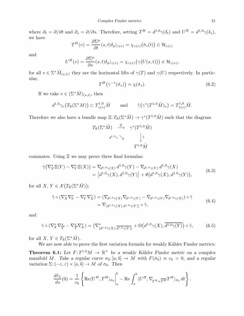
where ∂t = ∂/∂t and ∂s = ∂/∂s. Therefore, setting TH = d1,0γ(δt) and UH = d1,0γ(δs),

we have

TH(v) =∂Σµ

∂t(s, t)δµ|γ(v) = χγ(v)

(

σs(t))

∈ Hγ(v)

and

UH(v) =∂Σµ

∂s(s, t)δµ|γ(v) = χγ(v)

(

γ(

U(s, t)))

∈ Hγ(v),

for all v ∈ Σ∗M(s,t); they are the horizontal lifts of γ(T ) and γ(U) respectively. In partic-ular,

TH(

γ−1(σs))

= χ(σs). (6.2)

If we take v ∈ (Σ∗M)(s,t), then

d1,0γv(

TR(Σ∗M)

)

⊂ T 1,0γ(v)M and γ

(

γ∗(T 1,0M)v)

= T 1,0γ(v)M.

Therefore we also have a bundle map Ξ:TR(Σ∗M) → γ∗(T 1,0M) such that the diagram

TR(Σ∗M)

Ξ−→ γ∗(T 1,0M)

d1,0γ ց

y

γ

T 1,0M

commutes. Using Ξ we may prove three final formulas:

γ(

∇∗

XΞ(Y )−∇∗

Y Ξ(X))

= ∇d1,0γ(X) d1,0γ(Y )−∇d1,0γ(Y ) d

1,0γ(X)

=[

d1,0γ(X), d1,0γ(Y )]

+ θ(

d1,0γ(X), d1,0γ(Y ))

,(6.3)

for all X , Y ∈ X(

TR(Σ∗M)

)

;

γ (∇∗

X∇∗

Y −∇∗

Y ∇∗

X) = (∇d1,0γ(X)∇d1,0γ(Y ) −∇d1,0γ(Y )∇d1,0γ(X)) γ

= ∇[d1,0γ(X),d1,0γ(Y )] γ,(6.4)

and

γ (∇∗

X∇∗

Y−∇∗

Y∇∗

X) =(

∇∗

[d1,0γ(X),d1,0γ(Y )]+Ω

(

d1,0γ(X), d1,0γ(Y ))

γ, (6.5)

for all X , Y ∈ TR(Σ∗M).

We are now able to prove the first variation formula for weakly Kahler Finsler metrics:

Theorem 6.1: Let F :T 1,0M → R+ be a weakly Kahler Finsler metric on a complex

manifold M . Take a regular curve σ0: [a, b] → M with F (σ0) ≡ c0 > 0, and a regularvariation Σ: (−ε, ε)× [a, b] →M of σ0. Then

dℓΣds

(0) =1

c0

Re〈UH , TH〉σ0

∣

∣

∣

∣

b

a

− Re

∫ b

a

〈UH ,∇TH+THT

H〉σ0dt

.


In particular, if Σ is a fixed variation, that is Σ(·, a) ≡ σ0(a) and Σ(·, b) ≡ σ0(b), we have

dℓΣds

(0) = −1

c0Re

∫ b

a

〈UH ,∇TH+THT

H〉σ0dt. (6.6)

Proof : By definition,

ℓΣ(s) =

∫ b

a

(

G(σs))1/2

dt;

thereforedℓΣds

=1

2cs

∫ b

a

∂

∂s[G(σs)] dt =

1

2cs

∫ b

a

∂

∂s〈Ξ(δt),Ξ(δt)〉T dt,

where cs ≡ F (σs) and we used

G(σs) = 〈χ(σs), χ(σs)〉σs= 〈Ξ(δt),Ξ(δt)〉T ,

by (6.2). Now, using (6.1) and (6.3), we get

1

2

∂

∂s〈Ξ(δt),Ξ(δt)〉T =

1

2δs〈Ξ(δt),Ξ(δt)〉T

=1

2

〈∇∗

δsΞ(δt),Ξ(δt)〉T + 〈Ξ(δt),∇

∗

δsΞ(δt)〉T

+ 〈∇∗

δsΞ(δt),Ξ(δt)〉T + 〈Ξ(δt),∇

∗

δsΞ(δt)〉T

= Re

〈∇∗

δsΞ(δt),Ξ(δt)〉T + 〈∇∗

δsΞ(δt),Ξ(δt)〉T

= Re

〈∇∗

δtΞ(δs),Ξ(δt)〉T + 〈[UH , TH ] +∇UHT

H , TH〉σs+ 〈θ(UH , TH), TH〉σs

.

Since F is weakly Kahler, (6.2) yields

〈θ(UH , TH), TH〉σs= 0.

Furthermore,

[UH , TH ] =

∂Σν

∂sδν

(

∂Σµ

∂t

)

−∂Σν

∂tδν

(

∂Σµ

∂s

)

δµ,

∇UHT

H =∂Σν

∂sδν

(

∂Σµ

∂t

)

δµ;

since

∂Σν

∂sδν

(

∂Σµ

∂t

)

+∂Σν

∂sδν

(

∂Σµ

∂t

)

=∂2Σµ

∂s∂t=∂2Σµ

∂t∂s=∂Σν

∂tδν

(

∂Σµ

∂s

)

+∂Σν

∂tδν

(

∂Σµ

∂s

)

,

(6.7)we get

[UH , TH ] +∇UHT

H =∂Σν

∂tδν

(

∂Σµ

∂s

)

δµ = ∇THU

H . (6.8)


Then1

2

∂

∂s〈Ξ(δt),Ξ(δt)〉T = Re

〈∇∗

δtΞ(δs),Ξ(δt)〉T + 〈∇∗

δtΞ(δs),Ξ(δt)〉T

= Re

δt〈Ξ(δs),Ξ(δt)〉T − 〈Ξ(δs),∇∗

δt+δtΞ(δt)〉T

= Re

∂

∂t〈UH , TH〉σs

− 〈UH ,∇TH+THT

H〉σs

,

(6.9)

and the assertion follows.

As a corollary we get the equation of geodesics:

Corollary 6.2: Let F :T 1,0M → R+ be a weakly Kahler Finsler metric on a complex

manifold M , and let σ: [a, b] → M be a regular curve with F (σ) ≡ c0 > 0. Then σ is ageodesic for F iff

∇TH+THT

H ≡ 0, (6.10)

where TH(v) = χv

(

σ(t))

∈ Hv for all v ∈ Mσ(t).

Proof : It follows immediately from (6.6).

Corollary 6.3: Let F :T 1,0M → R+ be a weakly Kahler Finsler metric on a complex

manifold M . Then for any p ∈ M and v ∈ Mp with F (v) = 1 there exists a uniquegeodesic σ: (−ε, ε) →M such that σ(0) = p and σ(0) = v.

Proof : In local coordinates we have

∇TH+THT

H =[

(σµδµ + σµδµ)(σα) + Γα

ν;µ(σ)σµσν

]

δα = [σα + Γα;µ(σ)σ

µ]δα.

So (6.10) is a quasi-linear O.D.E. system, and the assertion follows.

Thus the standard O.D.E. arguments apply in this case too, and we may recover forweakly Kahler Finsler metrics the usual theory of geodesics. In particular, if the metric Fis complete we can define the exponential map expp:T

1,0p M →M for any p ∈M . See [AP4]

for details.

7. Second variation of the length integral

Our next goal is the second variation formula, which holds for Kahler Finsler metrics.To express it correctly, we need two further ingredients. The first one is the horizontal(1,1)-torsion τH , simply defined by

τH(X, Y ) = Θ(

τ(X, Y ))

= Ω(X, Y )χ.

The second one is the symmetric product 〈〈 , 〉〉:H×H → C locally given by

∀H,K ∈ Hv 〈〈H,K〉〉v = Gαβ(v)HαKβ.

It is clearly globally well-defined, and it satisfies

∀H ∈ H 〈〈H,χ〉〉 = 0.


Theorem 7.1: Let F :T 1,0M → R+ be a Kahler Finsler metric on a complex manifoldM .

Take a geodesic σ0: [a, b] →M with F (σ0) ≡ 1, and let Σ: (−ε, ε)× [a, b] →M be a regularvariation of σ0. Then

d2ℓΣds2

(0) = Re〈∇UH+UHU

H , TH〉σ0

∣

∣

∣

∣

b

a

+

∫ b

a

∥

∥∇TH+THU

H∥

∥

2

σ0

−

∣

∣

∣

∣

∂

∂tRe〈UH , TH〉σ0

∣

∣

∣

∣

2

− Re[

〈Ω(TH , UH)UH , TH〉σ0− 〈Ω(UH , TH)UH , TH〉σ0

+ 〈〈τH(UH , TH), UH〉〉σ0− 〈〈τH(TH , UH), UH〉〉σ0

]

dt.

In particular, if Σ is a fixed variation such that Re〈UH , TH〉σ0is constant we have

d2ℓΣds2

(0) =

∫ b

a

∥

∥∇TH+THU

H∥

∥

2

σ0

− Re[

〈Ω(TH , UH)UH , TH〉σ0− 〈Ω(UH , TH)UH , TH〉σ0

+ 〈〈τH(UH , TH), UH〉〉σ0− 〈〈τH(TH , UH), UH〉〉σ0

]

dt.

Proof : During the proof of the first variation formula — in (6.9) — we saw that

dℓΣds

(s) = Re

∫ b

a

〈∇∗



(

〈Ξ(δt),Ξ(δt)〉T)1/2

dt.

So we need to compute

∂

∂s

[〈∇∗



(

〈Ξ(δt),Ξ(δt)〉T)1/2

]

=δs〈∇

∗

δtΞ(δs),Ξ(δt)〉T + δs〈∇

∗


(

〈Ξ(δt),Ξ(δt)〉T)1/2

−1

2

〈∇∗



(

〈Ξ(δt),Ξ(δt)〉T)3/2

δs〈Ξ(δt),Ξ(δt)〉T .

(7.1)

Since, when s = 0, the denominator of the first term is equal to 1, and the denominatorof the second term is equal to 2, we may forget them. Let us call (I) the numerator of thefirst term, and (II) the numerator of the second term. First of all, (6.9) yields

1

2Re (II) =

∣

∣

∣

∣

Re

[

∂

∂t〈UH , TH〉σs

− 〈UH ,∇TH+THT

H〉σs

]∣

∣

∣

∣

2

;


in particular, for s = 0 we get

1

2Re (II)(0) =

∣

∣

∣

∣

∂

∂tRe〈UH , TH〉σ0

∣

∣

∣

∣

2

, (7.2)

because σ0 is a geodesic.The computation of (I) is quite longer. First of all, using (6.3), (6.4) and (6.5) we get

(I) = 〈∇∗

δs∇∗


δs∇∗


+ 〈∇∗

δtΞ(δs),∇

∗

δsΞ(δt)〉T + 〈∇∗

δtΞ(δs),∇

∗

δsΞ(δt)〉T

+ 〈∇∗

δs∇∗


δs∇∗


+ 〈∇∗

δtΞ(δs),∇

∗

δsΞ(δt)〉T + 〈∇∗

δtΞ(δs),∇

∗

δsΞ(δt)〉T

= 〈∇∗

δt∇∗

δsΞ(δs),Ξ(δt)〉T − 〈∇[TH ,UH ]U

H , TH〉σs

+ 〈∇∗

δt∇∗

δsΞ(δs),Ξ(δt)〉T − 〈∇

[TH ,UH ]UH , TH〉σs

− 〈Ω(TH , UH)UH , TH〉σs

+ 〈∇∗

δtΞ(δs),∇

∗

δtΞ(δs)〉T + 〈∇THUH , [UH , TH ] +∇

UHTH〉σs

+ 〈∇THUH , θ(UH , TH)〉σs

+ 〈∇∗

δt∇∗

δsΞ(δs),Ξ(δt)〉T − 〈∇[TH ,UH ]

UH , TH〉σs+ 〈Ω(UH , TH)UH , TH〉σs

+ 〈∇∗

δt∇∗

δsΞ(δs),Ξ(δt)〉T − 〈∇

[TH ,UH ]UH , TH〉σs

+ 〈∇∗

δtΞ(δs),∇

∗

δtΞ(δs)〉T + 〈∇THU

H , [UH , TH ] +∇UHT

H〉σs

+ 〈∇THU

H , θ(UH , TH)〉σs.

Recalling (6.8), (6.2) and that F is Kahler we get

(I) = 〈∇∗

δt∇∗

δsΞ(δs),Ξ(δt)〉T + 〈∇∗

δt∇∗

δsΞ(δs),Ξ(δt)〉T

+ 〈∇∗

δt∇∗

δsΞ(δs),Ξ(δt)〉T + 〈∇∗

δt∇∗

δsΞ(δs),Ξ(δt)〉T

− 〈Ω(TH , UH)UH , TH〉σs+ 〈Ω(UH , TH)UH , TH〉σs

− 〈∇[TH ,UH ]+[TH ,UH ]+[TH ,UH ]+[TH ,UH ]

UH , TH〉σs

+ 〈∇∗

δtΞ(δs),∇∗

δtΞ(δs)〉T + 〈∇∗

δtΞ(δs),∇

∗

δtΞ(δs)〉T

+ 〈∇∗

δtΞ(δs),∇

∗

δtΞ(δs)〉T + 〈∇∗

δtΞ(δs),∇

∗

δtΞ(δs)〉T .

Now

[TH , UH ] =

[

∂Σµ

∂tδµ

(

∂Σν

∂s

)

−∂Σµ

∂sδµ

(

∂Σν

∂t

)]

δν ,

[TH , UH ] =∂Σµ

∂t

∂Σν

∂s

[

δν(Γα;µ)∂α − δµ(Γ

β;ν)∂β

]

+∂Σµ

∂tδµ

(

∂Σν

∂s

)

δν −∂Σν

∂sδν

(

∂Σµ

∂t

)

δµ,

[TH , UH ] =∂Σµ

∂t

∂Σν

∂s

[

δν(Γβ;µ)∂β − δµ(Γ

α;ν)∂α

]

+∂Σµ

∂tδµ

(

∂Σν

∂s

)

δν −∂Σν

∂sδν

(

∂Σµ

∂t

)

δµ,

[TH , UH ] =

[

∂Σµ

∂tδµ

(

∂Σν

∂s

)

−∂Σµ

∂sδµ

(

∂Σν

∂t

)]

δν ,


and so (6.7) and (3.1) yield

[TH , UH ] + [TH , UH ] + [TH , UH ] + [TH , UH ]

= τ(UH , TH)− τ(TH , UH) + τ(UH , TH)− τ(TH , UH).

Furthermore, if V ∈ V we have

〈∇V UH , TH〉σs

= Gαβ(σs)Vγ

[

∂γ

(

∂Σα

∂s

)

+ Γαδγ(σs)

(

∂Σδ

∂s

)]

σβs

= Gα(σs)Γαδγ(σs)

(

∂Σδ

∂s

)

V γ = Gδγ(σs)

(

∂Σδ

∂s

)

V γ

= 〈〈Θ(V ), UH〉〉σs,

and

〈∇V UH , TH〉σs

= Gαβ(σs)Vγ

[

∂γ

(

∂Σα

∂s

)]

σβs

= 0.

Therefore

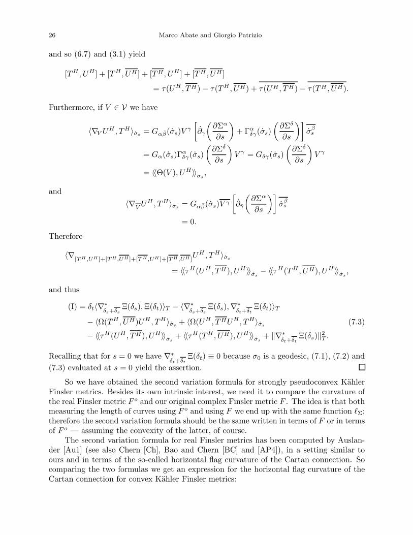
〈∇[TH ,UH ]+[TH ,UH ]+[TH ,UH ]+[TH ,UH ]

UH , TH〉σs

= 〈〈τH(UH , TH), UH〉〉σs− 〈〈τH(TH , UH), UH〉〉σs

,

and thus

(I) = δt〈∇∗

δs+δsΞ(δs),Ξ(δt)〉T − 〈∇∗

δs+δsΞ(δs),∇

∗

δt+δtΞ(δt)〉T

− 〈Ω(TH , UH)UH , TH〉σs+ 〈Ω(UH , THUH , TH〉σs

− 〈〈τH(UH , TH), UH〉〉σs+ 〈〈τH(TH , UH), UH〉〉σs

+ ‖∇∗

δt+δtΞ(δs)‖

2T .

(7.3)

Recalling that for s = 0 we have ∇∗

δt+δtΞ(δt) ≡ 0 because σ0 is a geodesic, (7.1), (7.2) and

(7.3) evaluated at s = 0 yield the assertion.

So we have obtained the second variation formula for strongly pseudoconvex KahlerFinsler metrics. Besides its own intrinsic interest, we need it to compare the curvature ofthe real Finsler metric F o and our original complex Finsler metric F . The idea is that bothmeasuring the length of curves using F o and using F we end up with the same function ℓΣ;therefore the second variation formula should be the same written in terms of F or in termsof F o — assuming the convexity of the latter, of course.

The second variation formula for real Finsler metrics has been computed by Auslan-der [Au1] (see also Chern [Ch], Bao and Chern [BC] and [AP4]), in a setting similar toours and in terms of the so-called horizontal flag curvature of the Cartan connection. Socomparing the two formulas we get an expression for the horizontal flag curvature of theCartan connection for convex Kahler Finsler metrics:


Corollary 7.2: Let F :T 1,0M → R+ be a convex (i.e., with strongly convex indicatrices)

Kahler Finsler metric on a complex manifold M . Then the horizontal flag curvature of theCartan connection associated to F o is given by

Rv(H,H) = Re[

〈Ω(χ,H)H,χ〉v − 〈Ω(H, χ)H,χ〉v

+ 〈〈τH(H, χ), H〉〉v − 〈〈τH(χ,H), H〉〉v

]

for all H ∈ H.

We shall need this result to apply Auslander’s version [Au2] of the classical Cartan-Hadamard theorem. By the way, it turns out that a direct computation of the Cartanconnection (and its curvature) in terms of the Chern-Finsler connection (and its curvature)is unexpectedly difficult; see [AP4] for details.

8. Manifolds with constant holomorphic curvature

A very natural problem now is the classification of Kahler Finsler manifolds of constantholomorphic curvature. In this respect, the Finsler situation is much richer than thehermitian one; for instance, Lempert’s work [Le] and [AP2] imply that all strongly convexdomains of Cn endowed with the Kobayashi metric are weakly Kahler Finsler manifoldswith constant holomorphic curvature −4.

The last theorem of this paper is a step toward this classification; roughly speaking,we shall prove that a simply connected Kahler Finsler manifold of nonpositive constantholomorphic curvature is diffeomorphic to an euclidean space. Furthermore, in the caseof constant negative holomorphic curvature our results show that the Finsler geometry ofthe manifold is pretty much the same of the one of strongly convex domains endowed withthe Kobayashi metric.

The idea is to apply the Cartan-Hadamard theorem; to do so, we need to estimatethe curvature terms appearing in the second variation formula.

Let F :T 1,0M → R+ be a strongly pseudoconvex Finsler metric on a complex mani-

fold M . We say that F has constant holomorphic curvature 2c ∈ R if

〈Ω(χ, χ)χ, χ〉 ≡ cG2, (8.1)

that is iff KF ≡ 2c. The idea is to differentiate (8.1) in such a smart way to get all theinformations we need.

We start with a couple of computational lemmas.

Lemma 8.1: Let F :T 1,0M → R+ be a strongly pseudoconvex Finsler metric on a complex

manifold M . Then

〈(∇WΩ)(H,K)χ, χ〉 = 〈τH(

H, θ(K,W ))

, χ〉

for all W ∈ V and H, K ∈ H. In particular,

〈(∇WΩ)(H, χ)χ, χ〉 = 0


for all W ∈ V and H ∈ H.

Proof : Since we are interested only in the horizontal part, we may replace Ω by

ΩH = Ωαβ ⊗ dzβ ⊗ δα.

Since ∇W dzβ = 0 and ∇W δα = 0, we have

∇WΩH = (∇WΩαβ )⊗ dzβ ⊗ δα.

Again, we only need the horizontal part, that is

p∗H(∇WΩαβ) =W (Rα

β;µν) dzµ ∧ dzν −Rα

β;µρ ωρν(W ) dzµ ∧ dzν .

Recalling (4.2), taking H, K, L ∈ H we get

〈(∇WΩH(H,K)L, χ〉 = Gα

[

W (Rαβ;µν)−Rα

β;µρ ωρν(W )

]

HµKνLβ

= −Gα

[

∂γδν(Γαβ;µ)− δρ(Γ

αβ;µ)Γ

ρνγ + ∂γ

(

Γαβσδν(Γ

σ;µ))

− Γαβσδρ(Γ

σ;µ)Γ

ρνγ

]

HµKνLβW γ

= −Gα

[

δν ∂γ(Γαβ;µ)− Γτ

γ;ν ∂τ (Γαβ;µ) + ∂γ(Γ

αβσ)δν(Γ

σ;µ) + δν(Γ

σγ;µ)Γ

αβσ

− ΓαβσΓ

τγ;νΓ

στ ;µ − δρ(Γ

αβ;µ)Γ

ρνγ − Γα

βσδρ(Γσ;µ)Γ

ρνγ

]

HµKνLβW γ

(where Γσγ;µ = ∂γ(Γ

σ;µ) and we used Lemma 2.1.(ii)),

= −[

δν(

Gα∂β(Γαγ;µ)

)

− Γτγ;νGα∂β(Γ

ατ ;µ) +Gβσδν(Γ

σγ;µ)−GβσΓ

τγ;νΓ

στ ;µ

− δρ(GαΓαβ;µ)Γ

ρνγ −Gβσδρ(Γ

σ;µ)Γ

ρνγ

]

HµKνLβW γ

(where we used GαΓαβσ = Gβσ, δν(Gα) = 0 and Gα∂γ(Γ

αβσ) = Gβσγ −GαγΓ

αβσ = 0),

= −[

−δν(GαβΓαγ;µ) + Γτ

γ;νGαβΓατ ;µ +Gβσδν(Γ

σγ;µ)−GβσΓ

τγ;νΓ

στ ;µ

− δρ(GαΓαβ;µ)Γ


σ;µ)Γ

ρνγ

]

HµKνLβW γ

(where we used GαΓατ ;µ = 0),

= −[

−δν(GαβΓαγ;µ) +Gβσδν(Γ

σγ;µ)− δρ(GαΓ

αβ;µ)Γ


σ;µ)Γ

ρνγ

]

HµKνLβW γ .

Hence

〈(∇WΩ)(H,K)χ, χ〉

= −[

−δν(GαβΓαγ;µ) +Gβσδν(Γ

σγ;µ)− δρ(GαΓ

αβ;µ)Γ


σ;µ)Γ

ρνγ

]

vβHµKνW γ ,

= δρ(GαΓα;µ)Γ

ρνγH

µKνW γ ,

(where we used (1.3) and vβΓαβ;µ = Γα

;µ),

= Gαδρ(Γα;µ)Γ

ρνγH

µKν W γ = 〈τH(

H, θ(K,W ))

, χ〉,

because θ(K,W ) = −Γρνγ K

νW γδρ, by (3.1).Finally,

〈(∇WΩ)(H, χ)χ, χ〉 = Gαδρ(Γα;µ)Γ

ρνγv

νHµW γ

= 0,

because Γρνγv

ν = 0.



manifold M . Then

〈(∇V Ω)(H,K)χ, χ〉 = 〈τH(

θ(H, V ), K)

, χ〉

for all V ∈ V and H, K ∈ H. In particular,

〈(∇VΩ)(χ,K)χ, χ〉 = 0

for all V ∈ V and K ∈ H.

Proof : Again it suffices to consider ΩH = Ωαβ ⊗ dzβ ⊗ δα; so

∇V ΩH = (∇V Ω

αβ )⊗ dzβ ⊗ δα − Ωα

γ ⊗ ωγβ(V ) dzβ ⊗ δα + Ωγ

β ⊗ dzβ ⊗ ωαγ (V )δα.

We are interested only in the horizontal part. Taking H, K ∈ H we get

Gα(∇V Ωαβ )(H,K) = Gα

[

V (Rαβ;µν)−Rα

β;ρνωρν(V )

]

HµKν

= −Gα

[

∂λδν(Γαβ;µ)− δν(Γ

αβ;ρ)Γ

ρµλ + ∂λ

(

Γαβσδν(Γ

σ;µ))

− Γαβσδν(Γ

σ;ρ)Γ

ρµλ

]

V λHµKν

= −Gα

[

δν ∂λ(Γαβ;µ)− Γτ

λ;ν ∂τ (Γαβ;µ)− δν(Γ

αβ;ρ)Γ

ρµλ + ∂λ(Γ

αβσ)δν(Γ

σ;µ) + Γα

βσδν(Γσλ;µ)

− ΓαβσΓ

στ ;µΓ

τλ;ν − Γα

βσδν(Γσ;ρ)Γ

ρµλ

]

V λHµKν

(where we used [δν , ∂λ] = Γτλ;ν ∂τ ),

= −[

δν(

Gα∂β(Γαλ;µ)

)

− Γτλ;νGα∂β(Γ

ατ ;µ)− δν(GαΓ

αβ;ρ)Γ

ρµλ +Gα∂λ(Γ

αβσ)δν(Γ

σ;µ)

+Gβσδν(Γσλ;µ)−GβσΓ

στ ;µΓ

τλ;ν −Gβσδν(Γ

σ;ρ)Γ

ρµλ

]

V λHµKν

(where we used δν(Gα) = 0 and GαΓαβσ = Gβσ),

= −[

−δν(GαβΓαλ;µ) + δν

(

∂βδµ(Gλ))

+ Γτλ;νGαβΓ

ατ ;µ − δν(GαΓ

αβ;ρ)Γ

ρµλ

+Gα∂λ(Γαβσ)δν(Γ

σ;µ) +Gβσδν(Γ

σλ;µ)−GβσΓ

στ ;µΓ

τλ;ν −Gβσδν(Γ

σ;ρ)Γ

ρµλ

]

V λHµKν

(where we used GαΓατ ;µ = 0 and GαΓ

αλ;µ = δµ(Gλ)),

= −[


(

∂βδµ(Gλ))

− δν(GαΓαβ;ρ)Γ

ρµλ +Gα∂λ(Γ

αβσ)δν(Γ

σ;µ)

+Gβσδν(Γσλ;µ)−Gβσδν(Γ

σ;ρ)Γ

ρµλ

]

V λHµKν .

Furthermore,

GαΩαγ (H,K)ωγ

β(V ) = −Gα

[

δν(Γαγ;µ) + Γα

γσδν(Γσ;µ)]

ΓγβλV

λHµKν

= −[

δν(

δµ(Gγ))

+Gγσδν(Γσ;µ)]

ΓγβλV

λHµKν ;

Gα ωαγ (V )Ωγ

β(H,K) = −GαΓαγλ

[

δν(Γγβ;µ) + Γγ

βσδν(Γσ;µ)]

V λHµKν

= −Gγν

[

δν(Γγβ;µ) + Γγ

βσδν(Γσ;µ)]

V λHµKν .


Summing up we find

〈(∇V Ω)(H,K)χ, χ〉

= −[


(

∂βδµ(Gλ))

− δν(GαΓαβ;ρ)Γ

ρµλ +Gα∂λ(Γ

αβσ)δν(Γ

σ;µ)

+Gβσδν(Γσλ;µ)−Gβσδν(Γ

σ;ρ)Γ

ρµλ + δν

(

δµ(Gγ))

Γγβλ +Gγσδν(Γ

σ;µ)Γ

γβλ +Gγνδν(Γ

γβ;µ)

+GγνΓγβσδν(Γ

σ;µ)]

vβV λHµKν

= −[

δν(

vβ∂βδµ(Gλ))

− δν(GαvβΓα

β;ρ)Γρµλ +Gαv

β∂λ(Γαβσ)δν(Γ

σ;µ)

+Gγλδν(Γγ;µ)]

V λHµKν

= −[

−δν(G;ρ)Γρµλ −Gλσδν(Γ

σ;µ) +Gλγδν(Γ

γ;µ)]

V λHµKν

(where we used vβ∂βδµ(Gλ) = vβGλβ;µ − vβΓσβ;µGλσ − vβΓσ

;µGλσβ = 0),

= δν(G;ρ)ΓρµλV

λHµKν = δν(GσΓσ;ρ)Γ

ρµλV

λHµKν

= Gσδν(Γσ;ρ)Γ

ρµλV

λHµKν = 〈τH(

θ(H, V ), K)

, χ〉.

The final assertion follows from θ(χ, V ) = 0.

In the following computations we shall need some symmetries of the curvature oper-ator, summarized in


manifold M . Then

(i) 〈Ω(H, χ)χ, χ〉 = 〈Ω(χ, χ)H,χ〉 for all H ∈ H iff

〈∂Hθ(H,χ, χ), χ〉 = 0 (8.2)

for all H ∈ H;(ii) 〈Ω(H,K)χ, χ〉 = 〈Ω(χ,K)H,χ〉 for all H, K ∈ H iff

〈∂Hθ(H,χ,K), χ〉 = 0 (8.3)

for all H, K ∈ H.

Proof : It follows immediately from (5.4) and Proposition 4.1.

Now we can start. The first step is:

Proposition 8.4: Let F :T 1,0M → R+ be a strongly pseudoconvex Finsler metric on a

complex manifold M , with constant holomorphic curvature 2c ∈ R. Then

〈∂Hθ(H,χ, χ), χ〉 = 0 (8.4)

for all H ∈ H iff

τH(χ, χ) = cGχ. (8.5)


Furthermore, they both imply

〈Ω(χ,K)χ, χ〉 = cG〈χ,K〉 (8.6)

for all K ∈ H.

Proof : TakeW ∈ V and let K = Θ(W ) ∈ H; note that ∇Wχ = 0 and ∇W

χ = Θ(W ) = K.Then

W (cG2) = 2cG〈χ,K〉;

W 〈Ω(χ, χ)χ, χ〉 = 〈(∇WΩ)(χ, χ)χ, χ〉+ 〈Ω(χ,K)χ, χ〉+ 〈Ω(χ, χ)χ,K〉

= 〈Ω(χ,K)χ, χ〉+ 〈τH(χ, χ), K〉,

(8.7)

where we used Lemmas 8.1 and 4.2. Since F has constant holomorphic curvature 2c, wehave

〈Ω(χ, χ)χ, χ〉 = cG2

and hence (8.7) yields

〈Ω(χ,K)χ, χ〉 = 2cG〈χ,K〉 − 〈τH(χ, χ), K〉. (8.8)

Subtracting 〈τH(χ, χ), K〉 = 〈Ω(χ, χ)χ,K〉 to both sides, we find that (8.5) holds if andonly if

〈ΩH(χ,K)χ, χ〉 = 〈ΩH(χ, χ)χ,K〉

for all K ∈ H, that is, recalling (5.5), iff

〈Ω(K, χ)χ, χ〉 = 〈Ω(χ, χ)K,χ〉,

and thus, by Lemma 8.3, iff (8.4) holds.Finally, if (8.5) holds, (8.8) yields (8.6).

The second step requires (8.3):


complex manifold M with constant holomorphic curvature 2c ∈ R. Assume that (8.2)holds. Then

〈Ω(H,K)χ, χ〉+ 〈Ω(χ,K)H,χ〉 = c 〈H,χ〉〈χ,K〉+ 〈χ, χ〉〈H,K〉 , (8.9)

for all H, K ∈ H. In particular, if (8.3) holds then

〈Ω(χ,K)H,χ〉 =c

2〈H,χ〉〈χ,K〉+ 〈χ, χ〉〈H,K〉 (8.10)

for all H, K ∈ H.

Proof : Take V , W ∈ V such that Θ(V ) = H and Θ(W ) = K and extend them in any wayto sections of V (and thus extend H and K as sections of H via Θ). We have

V(

cG〈χ,K〉) = c[

〈H,χ〉〈χ,K〉+G〈H,K〉+G〈χ,∇VK〉]

,


and

V 〈Ω(χ,K)χ, χ〉

= 〈(∇V Ω)(χ,K)χ, χ〉+ 〈Ω(H,K)χ, χ〉+ 〈Ω(χ,∇VK)χ, χ〉+ 〈Ω(χ,K)H,χ〉

= 〈Ω(H,K)χ, χ〉+ 〈Ω(χ,∇VK)χ, χ〉+ 〈Ω(χ,K)H,χ〉,

thanks to Lemma 8.2. Since (8.2) holds, we can use Lemma 8.4 (that is, (8.6) applied bothto K and to ∇VK) to get exactly (8.9).

Finally, (8.10) follows from Lemma 8.3.

So we have obtained one of the hermitian product terms. This immediately yields oneof the symmetric product terms:



τH(K, χ) =c

2〈K,χ〉χ+ 〈χ, χ〉K (8.11)

for all K ∈ H. In particular,

〈〈H, τH(K, χ)〉〉 =c

2〈χ, χ〉〈〈H,K〉〉 (8.12)

for all H, K ∈ H.

Proof : We get〈H, τH(K, χ)〉 = 〈H,Ω(K, χ)χ〉 = 〈Ω(χ,K)H,χ〉

for all H, K ∈ H, thanks to Lemma 4.2 and (5.5). Then (8.10) yields (8.11), and (8.12)follows immediately.

For the other symmetric product term we need the weak Kahler condition:

Proposition 8.7: Let F :T 1,0M → R+ be a weakly Kahler-Finsler metric on a complex

manifold M such that (8.3) holds. Then

〈〈H, τH(χ,K)〉〉 = 0

for all H, K ∈ H.

Proof : The weak Kahler condition 〈θ(H,χ), χ〉 = 0 for all H ∈ H implies

∀H, K ∈ H 〈(∇Kθ)(H,χ), χ〉 = 0 (8.13)

because ∇Kχ = 0 = ∇K

χ. Now, writing θ = θα ⊗ δα, we have ∇Kθ = (∇Kθα)⊗ δα and

∇Kθα = Kτ δτ (Γ

αν;µ) dz

µ ∧ dzν +Kτ δτ (Γανγ)ψ

γ ∧ dzν .

Therefore (8.13) implies

Gα[δτ (Γαν;µ)− δτ (Γ

αµ;ν)]H

µKτvν = 0 (8.14)


for all H, K ∈ H.Writing the curvature in local coordinates we find

〈Ω(χ,K)H,χ〉 = −Gα[δτ (Γαµ;ν) + Γα

µσδτ (Γσ;ν)]H

µKτvν ,

〈Ω(H,K)χ, χ〉 = −Gα[δτ (Γαν;µ) + Γα

νσδτ (Γσ;µ)]H

µKτvν .

So (8.14) yields

〈Ω(χ,K)H,χ〉 − 〈Ω(H,K)χ, χ〉 = −GαΓαµσδτ (Γ

σ;ν)H

µKτvν

= 〈〈H, τH(χ,K)〉〉,

and the assertion follows from (8.3).

We are left with the last term:



〈Ω(H, χ)K,χ〉 = c 〈H,χ〉〈K,χ〉+ 〈χ, χ〉〈〈H,K〉〉

for all H, K ∈ H.

Proof : First of all, we have

〈Ω(H, χ)χ, χ〉 = 〈χ,Ω(χ,H)χ〉 = 〈Ω(χ,H)χ, χ〉 = cG〈H,χ, 〉, (8.15)

by (5.5) and (8.6). Now take W ∈ V such that Θ(W ) = K; then

W (cG〈H,χ〉) = c 〈K,χ〉〈H,χ〉+G〈∇WH,χ〉 ,

W 〈Ω(H, χ)χ, χ〉 = 〈(∇WΩ)(H, χ)χ, χ〉+ 〈Ω(∇WH, χ)χ, χ〉+ 〈Ω(H, χ)K,χ〉,

and so (8.15) yields

〈Ω(H, χ)K,χ〉 = c〈K,χ〉〈H,χ〉 − 〈(∇WΩ)(H, χ)χ, χ〉.

Now Lemma 8.2 gives

〈(∇WΩ)(H, χ)χ, χ〉 = 〈τH(

θ(H,W ), χ)

, χ〉 = 〈Ω(

θ(H,W ), χ)χ, χ〉

= cG〈θ(H,W ), χ〉,

again by (8.15). But

〈θ(H,W ), χ〉 = −GαΓανβK

βHν = −〈〈H,K〉〉,

and we are done.

We can finally collect all our computations in


Corollary 8.9: Let F :T 1,0M → R+ be a weakly Kahler-Finsler metric on a complex

manifold M . Assume F has constant holomorphic curvature 2c ∈ R and that (8.3) holds.Then

Re[

〈Ω(χ,K)H,χ〉 − 〈Ω(H, χ)K,χ〉+ 〈〈H, τH(K, χ)〉〉 − 〈〈H, τH(χ,K)〉〉]

=c

2Re[

G

〈H,K〉 − 〈〈H,K〉〉

+ 〈H,χ〉

〈χ,K〉 − 2〈K,χ〉

]

for all H, K ∈ H.

Proof : It follows from Propositions 8.5, 8.6, 8.7, 8.8 and Corollary 7.2.

We are then able to prove the announced

Theorem 8.10: Let F :T 1,0M → R+ be a complete Finsler metric on a simply connected

complex manifold M . Assume that:

(i) F is Kahler;(ii) F has nonpositive constant holomorphic curvature 2c ≤ 0;(iii) 〈∂Hθ(H,χ,K), χ〉 = 0 for all H, K ∈ H;(iv) the indicatrices of F are strongly convex.

Then expp:T1,0p → M is a homeomorphism, and a smooth diffeomorphism outside the

origin, for any p ∈M . Furthermore,M is foliated by isometric totally geodesic holomorphicembeddings of the unit disk ∆ endowed with a suitable multiple of the Poincare metricif c < 0, or by isometric totally geodesic holomorphic embeddings of C endowed with theeuclidean metric if c = 0. In particular, if 2c = −4 then F is the Kobayashi metric of M ,and if c = 0 then the Kobayashi metric of M vanishes identically.

Proof : Let F o:TRM → R+ be the real Finsler metric associated to F as at the beginning

of section 6. Then Corollary 7.2 and Corollary 8.9 show that the horizontal flag curvatureof F o is given by

R(H,H) =c

2Re

G[

〈H,H〉 − 〈〈H,H〉〉]

+ 〈H,χ〉[

〈χ,H〉 − 2〈H,χ〉]

.

In particular, if H = χ we getR(χ, χ) = 0, (8.16)

and if 〈H,χ〉 = 0 we get

R(H,H) =cG

2Re[

〈H,H〉 − 〈〈H,H〉〉]

=cG

2Re[

〈iH, iH〉+ 〈〈iH, iH〉〉]

.

Now, in local coordinates the quadratic form

H 7→ Re[

〈H,H〉+ 〈〈H,H〉〉]

is represented by the Hessian of G; by (iv), it is positive definite. So 〈H,χ〉 implies

R(H,H) ≤ 0. (8.17)

Now, take K ∈ H and write K = ζχ+H, with 〈H,χ〉 = 0. Then Corollary 8.9, (8.16) and(8.17) yield

R(K,K) = R(H,H) ≤ 0.

In conclusion, the horizontal flag curvature is negative semi-definite, and the first assertionfollows from Auslander’s version of the Cartan-Hadamard theorem [Au2]. Finally, the lastassertion has been proved under weaker assumptions in [AP2, 3].


We remark that, contrarily to what happens in the hermitian case, condition (iii)does not seem to be a consequence of the Kahler condition. For instance, the proof ofProposition 8.7 shows that if F is weakly Kahler (but even Kahler does not help much)then condition (iii) holds iff

∀H, K ∈ H 〈〈H, τH(χ,K)〉〉 = 0.

References

[A] M. Abate: Iteration theory of holomorphic maps on taut manifolds. Medi-terranean Press, Cosenza, 1989.

[AP1] M. Abate, G. Patrizio: Uniqueness of complex geodesics and characterization ofcircular domains. Man. Math. 74 (1992), 277–297.

[AP2] M. Abate, G. Patrizio: Holomorphic curvature of Finsler metrics and complexgeodesics. To appear in J. Geom. Anal. (1993).

[AP3] M. Abate, G. Patrizio: Complex geodesics and Finsler metrics. To appear in Pro-ceedings of the Semester in Complex Analysis, Banach Center, Warsaw, 1992.

[AP4] M. Abate, G. Patrizio: A global approach to Finsler metrics. In preparation (1993).

[Au1] L. Auslander: On the use of forms in the variational calculations. Pac. J. Math.5 (1955), 853–859.

[Au2] L. Auslander: On curvature in Finsler geometry . Trans. Am. Math. Soc. 79 (1955),378–388.

[BC] D. Bao, S.S. Chern: On a notable connection in Finsler geometry . Houston J. Math.19 (1993), 138–180.

[B] A. Bejancu: Finsler geometry and applications. Ellis Horwood Limited, Chich-ester, 1990.

[C] E. Cartan: Les espaces de Finsler. Hermann, Paris, 1934.

[Ch] S.S. Chern: On Finsler geometry . C.R. Acad. Sc. Paris 314 (1992), 757–761.

[F] J.J. Faran: Hermitian Finsler metrics and the Kobayashi metric. J. Diff. Geom.31 (1990), 601–625.

[Fu] M. Fukui: Complex Finsler manifolds. J. Math. Kyoto Univ. 29 (1989), 609–624.

[JP] M. Jarnicki, P. Pflug: Invariant distances and metrics in complex analysis.

de Gruyter, Berlin, 1993.

[K1] S. Kobayashi: Invariant distances on complex manifolds and holomorphic mappings.J. Math. Soc. Japan 19 (1967), 460–480.

[K2] S. Kobayashi: Hyperbolic manifolds and holomorphic mappings. Dekker,New York, 1970.

[K3] S. Kobayashi: Negative vector bundles and complex Finsler structures. NagoyaMath. J. 57 (1975), 153–166.

[K4] S. Kobayashi: Intrinsic distances, measures and geometric function theory . Bull.Am. Math. Soc. 82 (1976), 357–416.


[KN] S. Kobayashi, K. Nomizu: Foundations of differential geometry, vol. II. Wiley,New York, 1969.

[L] S. Lang: An introduction to complex hyperbolic spaces. Springer, New York,1987.

[Le] L. Lempert: La metrique de Kobayashi et la representation des domaines sur laboule. Bull. Soc. Math. France 109 (1981), 427–474.

[M] M. Matsumoto: Foundations of Finsler geometry and special Finsler spaces.

Kaiseisha Press, Otsu Japan, 1966.

[P1] M.Y. Pang: Finsler metrics with the properties of the Kobayashi metric on convexdomains. Publications Mathematiques 36 (1992), 131–155.

[P2] M.Y. Pang: Smoothness of the Kobayashi metric of non-convex domains. Preprint(1993).

[R] H.L. Royden: Complex Finsler metrics. In Contemporary Mathematics. Pro-

ceedings of Summer Research Conference, American Mathematical Society,Providence, 1984, pp. 119–124.

[Ru1] H. Rund: The differential geometry of Finsler spaces. Springer, Berlin, 1959.

[Ru2] H. Rund: Generalized metrics on complex manifolds. Math. Nach. 34 (1967),55–77.

[S] M. Suzuki: The intrinsic metrics on the domains in Cn. Math. Rep. Toyama Univ.

6 (1983), 143–177.

[W] B. Wong: On the holomorphic sectional curvature of some intrinsic metrics. Proc.Am. Math. Soc. 65 (1977), 57–61.

[Wu] H. Wu: A remark on holomorphic sectional curvature. Indiana Math. J. 22 (1973),1103–1108.

complexfinslermetrics by marco abate and giorgio patrizio · by marco abate and giorgio patrizio...

Documents