complex wavelet transform based hyper analytical...

International Journal of Computer Trends and Technology (IJCTT) – Volume 43 Number 3, January 2017

ISSN: 2231-2803http://www.ijcttjournal.org

COMPLEX WAVELET TRANSFORM BASED HYPER ANALYTICAL IMAGE

DENOISING BY BIVARIATE SHRINKAGE TECHNIQUE

S.Sasi Pavan Kumar1 , Dr.T.Sreenivasulu Reddy2 1(Pg Scholar, Dept Of Electronics & Communication Engineering, SVU Engineering College, Tirupati)

[email protected] 2(Professor, Dept Of Electronics &Communication Engineering, SVU Engineering College, Tirupati)

[email protected]

Abstract—Removal of noise is an important step in the image restoration process, but de-noising of image remains a challenging problem in recent research associated with image processing.

De-noising is used to remove the noise from corrupted image, while retaining the edges and other detailed features as much as possible. This noise gets introduced during acquisition, transmission, reception, storage and retrieval processes. Here we retrieve de-noised image using Bivariate Shrinkage Technique. Out of many wavelet transforms here Discrete Wavelet Transform, Dual Tree Wavelet Transform and Hyper Analytical Wavelet transforms are implemented on different noisy images. Here the noisy image is assumed to be complex image and its real part and imaginary parts are separated. These are subjected to Bi-shrink filter separately into different stages of decomposition depending upon the severity of noise. The obtained de-noise image is compared with original image using different parametric measures like Peak Signal to Noise Ratio, Structural similarity Index measure, Covariance and Root mean square Error whose values are tabulated. The values of retrieved image obtained yields much better visual effect and hence this method is said to be a better one when compared with de-noising methods using Weiner Filter and various Local Adaptive Filters.

I. INTRODUCTION Digital images play an important role both in daily life

applications such as satellite television, computed tomography as well as in areas of research and technology such as geographical information systems and astronomy. In reality, an image is mixed with certain amount of noise which decreases visual quality of image[1][9]. Therefore, removal of noise in an image is a very common problem in recent research fields of image processing. An image gets corrupted with noise during acquisition or at transmission due to channel errors or errors in storage media due to faulty hardware[1][2]. Removing noise from the noisy image is

still a challenging problem for researchers. Noise may be classified as substitutive noise (impulsive noise: e.g., salt and pepper noise, random valued impulse noise etc.) additive noise (e.g., additive white Gaussian noise) and multiplicative noise (e.g. speckle noise). However, here the investigation has been limited to additive white Gaussian noise[1]. In general, the goal of any noise removal scheme is to suppress noise as well as to preserve details and edges of image as much as possible. Removal of noise is an important aspect in the image processing.

Figure. 1 shows the basic model for de-noising of image. In the implementation of these methods, first the noisy image is decomposed by wavelet transform. After this, by using Bivariate shrinkage technique the decomposed images are subjected to de-noising process where the output is given to Shrink Thresholding. Finally de-noised image is obtained by using inverse wavelet transform as shown in figure 1.

Figure: 1 Image de-noising Process using Bivariate

Shrinkage Technique

Consider an image is corrupted with additive Gaussian white noise. The noisy image can be modelled as: 𝑦(𝑖, 𝑗) = 𝑥(𝑖, 𝑗) + 𝑛(𝑖, 𝑗) (1) Where 𝑦(𝑖, 𝑗)is the noisy image,

𝑥(𝑖, 𝑗) is the original image and 𝑛(𝑖, 𝑗) is additive Gaussian white noise.

INPUT IMAGE + NOISE =

NOISY IMAGE

APPLY WAVELET

TRANSFORM

APPLY BIVARIATE SHRINKAGE TECHNIQUE

THRESHOLDING (SOFT & HARD)

APPLY INVERSE WAVELET

TRANSFORM

DENOISED IMAGE

http://www.ijcttjournal.org/

mailto:[email protected]

mailto:[email protected]

lalitha

Text Box

143

lalitha

Text Box

lalitha

Text Box



The goal of image de-noising is to suppress noise from noisy image with minimum mean square error. Here, the wiener filter minimizes the mean square error between the estimated image 𝑥(𝑖, 𝑗) and the original image 𝑥(𝑖, 𝑗)[1][7]. This error measure can be expressed as: 𝑒2 = 𝐸[(𝑥(𝑖, 𝑗) − 𝑥(𝑖, 𝑗))

2] (2)

Wiener filter is used to measure an image pixel by pixel and compares the neighbourhoods of size M-by-N to estimate the local image mean and standard deviation[1][7]. Here it assumes that the noise is stationary with zero mean and variance 𝜎𝑛

2 and uncorrelated with the original image 𝑥(𝑖, 𝑗) . Based on these assumptions wiener filter estimates local mean and variance around each pixel using (3) and (4) as below: 𝜇 =

1

𝑀𝑁∑ 𝑦(𝑖, 𝑗)𝑖,𝑗𝜖𝑘 (3)

𝜎2 =1

𝑀𝑁∑ 𝑦2(𝑖, 𝑗) − 𝜇2

𝑖,𝑗𝜖𝑘 (4) Where 𝜇 is local mean and 𝜎2 is local variance. Then wiener filter creates a pixel wise filtering

using these estimates and the estimated image is given in (5) as below:

𝑥(𝑖, 𝑗) = 𝜇 +𝜎2+𝜎𝑛

2

𝜎2(𝑦(𝑖, 𝑗) − 𝜇) (5)

Where 𝜎𝑛2 is noise variance, if noise variance is not

given, wiener filter uses average of all local estimated variances.

The Wiener filter in the wavelet domain removes the noise pretty well in the smooth regions but performs poorly along the edges. That is why it performs better on smooth images like Lena than on images with edges like the cameraman. For a noise variance of 400, the MSE was found to be 107.5 for the cameraman image and 80.5 for the Lena image.

In Global Wiener filtering, the above expression for a Wiener filter is applied over the whole image. This method does a good job at de-blurring; however, it behaves very poorly in the presence of large noise[2][3]. The Wiener filter would work well for an image which has similar local statistics throughout the entire image. However in most natural images, the first order statistics vary from one part of an image to another and hence its poor performance in the presence of large noise. The advantage of this method is that it is not computationally intensive and works well for smooth images[1][4].

When Wiener filtering is performed on small blocks of an image at a time, the method is called Local Wiener Filtering. In this method, the PSD (Power Spectral Density) of the unregarded image is estimated for each block[4]. This calculated PSD is then used in the expression of the Wiener filter. Thus, the local statistics are also accounted for in the calculation of the Wiener filtered image[6]. Images with many edges are handled much better by the local Wiener filter than the global Wiener filter. We used a window of size of 3 × 3 in the calculation of the local Wiener filtered image. The drawback of this method is that it is more computationally demanding[6][1].

The de-noising of the image is done in the following procedural steps. First select an image, check whether it is grey image or colour Image. If it is a colour

image then firstly convert this image into grey image. Then use it as input image[1][4]. The image is further decomposed into four stages

approximation, horizontal, vertical and diagonal versions. The horizontal, vertical and diagonal steps of the image are called details of the image.

The approximation step is further processed for decomposition. The approximation is further carried out and divided into four steps again for three decompositions.

The decomposed images are retrieved by comparing approximation coefficients and details coefficients. This process is carried out by preceding the decomposition levels. The coefficients obtained in first stage are considered as finally obtained ones.

The retrieved coefficients are then succeeded for soft thresholding and subjected to Inverse wavelet Transform.

Here we have considered Dual tree and Hyper Analytical wavelet transforms where the give image is considered as complex one and is sub divided into real and imaginary parts. The marginal variance of the coefficients of the image is calculated separately for both real and imaginary images[5]. Finally, calculate PSNR between original image and

noisy image and PSNR between the de-noised image and original image.

PROPOSED WORK

BIVARIATE SHRINKAGE FILTER Bivariate shrinkage model undergoes the following

calculations. There are strong dependencies between neighbour coefficients such as between a coefficient, its parent (adjacent coarser scale locations), and their siblings (adjacent spatial locations).

Let 𝑤2 represents the parent of 𝑤1 (𝑤2 is the wavelet coefficient at the same position as 𝑤1 , but at the next coarser scale.) Then

𝑦1 = 𝑤1 + 𝑛1 𝑦2 = 𝑤2 + 𝑛2

Where 𝑦1 and 𝑦2 are noisy observations of 𝑤1and 𝑤2, 𝑛1and𝑛2 are noise samples. We can write

y = w + n where w=(𝑤1,𝑤2), y = (𝑦1, 𝑦2) and n = (𝑛1, 𝑛2) The estimator for w given the corrupted observation y is

𝑊𝑠 = 𝑎𝑟𝑔𝑊𝑠𝑚𝑎𝑥(𝑃𝑊𝑥 𝑊𝑠⁄ (𝑊𝑥 𝑊𝑠)⁄

After some manipulations, this equation can be written as 𝑎𝑟𝑔𝑊𝑠

𝑚𝑎𝑥(𝑃𝑊𝑠 𝑊𝑥⁄ (𝑊𝑠 𝑊𝑥)⁄ ) 𝑎𝑟𝑔𝑊𝑠

𝑚𝑎𝑥(𝑃𝑛(𝑊𝑠 − 𝑊𝑥). 𝑃𝑊𝑠(𝑊𝑠)) (i)

For construction of Bi-shrink filter, Let us assume Gaussian noise is added to the given image then,

𝑝𝑤𝑛(𝑊𝑛) =

1

2𝜋𝜎𝑊𝑛2 𝑒

− (𝑊𝑛

1 )2

+(𝑊𝑛2 )

2

2𝜎𝑊𝑛2

For a noise free image it is characterised as,


lalitha

Text Box

144



𝑝𝑤𝑠(𝑊𝑠) =

3

2𝜋𝜎𝑊𝑠2 𝑒

− √3

𝜎𝑊𝑠√(𝑊𝑠

1)2

+(𝑊𝑠2)

2

By substituting the above equation in equation (i) we finally contain the relationship between input and output of the given images,

𝑊𝑠1̂ =

√(𝑊𝑥1)

2+(𝑊𝑥

2)2

− √3 𝜎𝑊𝑛

2

𝜎𝑊𝑠

√(𝑊𝑥1)

2+(𝑊𝑥

2)2

. 𝑊𝑥1

Where 𝜎𝑊𝑛2 =

𝑚𝑒𝑑𝑖𝑎𝑛 |𝑊𝑥|

0.6745

𝜎𝑊𝑠 = 𝜎𝑊𝑠

1 + 0.5𝜎𝑊𝑠2

2

COMPLEX WAVELET TRANSFORMS: The complex wavelet transform [11] is divided into

different sub transforms among them the following methods are applied for denoising process.

A. DISCRETE WAVELET TRANSFORMS: The DWT transform, to which we will refer to as

classical DWT, presented in section is the most commonly used as it is fast, non-redundant and assures the perfect reconstruction. Despite all these properties, classical DWT might not be good enough for some specific applications. In the following, we will present some transforms, derived from DWT, that can be encountered in practical applications.

DWT is largely used for one-dimensional discrete signals. If we want apply the discrete wavelet transform to two-dimensional signals (images, for instance), we need to use the DWT’s extension to two dimensions, namely the 2D

DWT.

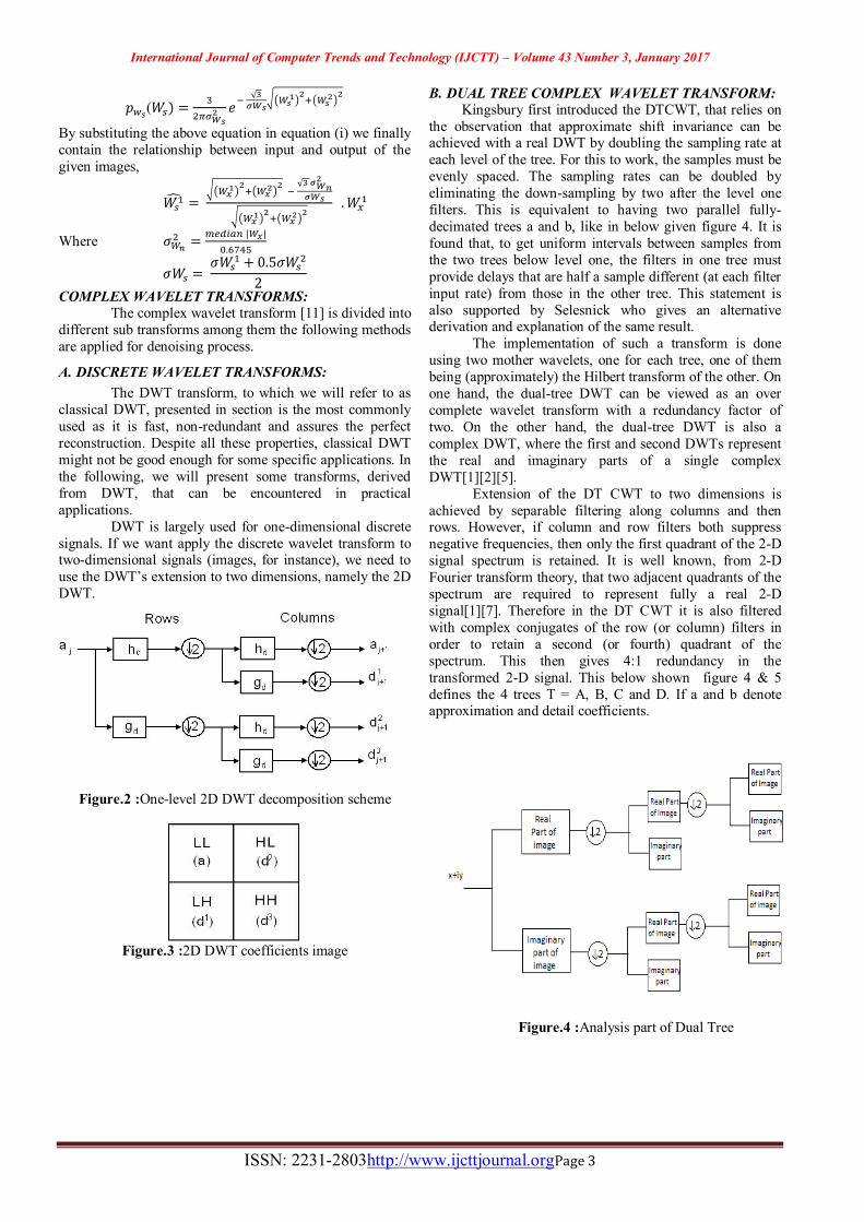
Figure.2 :One-level 2D DWT decomposition scheme

Figure.3 :2D DWT coefficients image

B. DUAL TREE COMPLEX WAVELET TRANSFORM: Kingsbury first introduced the DTCWT, that relies on

the observation that approximate shift invariance can be achieved with a real DWT by doubling the sampling rate at each level of the tree. For this to work, the samples must be evenly spaced. The sampling rates can be doubled by eliminating the down-sampling by two after the level one filters. This is equivalent to having two parallel fully-decimated trees a and b, like in below given figure 4. It is found that, to get uniform intervals between samples from the two trees below level one, the filters in one tree must provide delays that are half a sample different (at each filter input rate) from those in the other tree. This statement is also supported by Selesnick who gives an alternative derivation and explanation of the same result. The implementation of such a transform is done using two mother wavelets, one for each tree, one of them being (approximately) the Hilbert transform of the other. On one hand, the dual-tree DWT can be viewed as an over complete wavelet transform with a redundancy factor of two. On the other hand, the dual-tree DWT is also a complex DWT, where the first and second DWTs represent the real and imaginary parts of a single complex DWT[1][2][5]. Extension of the DT CWT to two dimensions is achieved by separable filtering along columns and then rows. However, if column and row filters both suppress negative frequencies, then only the first quadrant of the 2-D signal spectrum is retained. It is well known, from 2-D Fourier transform theory, that two adjacent quadrants of the spectrum are required to represent fully a real 2-D signal[1][7]. Therefore in the DT CWT it is also filtered with complex conjugates of the row (or column) filters in order to retain a second (or fourth) quadrant of the spectrum. This then gives 4:1 redundancy in the transformed 2-D signal. This below shown figure 4 & 5 defines the 4 trees T = A, B, C and D. If a and b denote approximation and detail coefficients.

Figure.4 :Analysis part of Dual Tree


lalitha

Text Box

145



Figure.5 : Synthesis part of Dual tree

Figure.6: Approximation components at levels 1 to

4 of 16 shifted step responses of the (a) DT CWT and (b) Real DWT

C. HYPER ANALYTICAL WAVELET TRANSFORM: In the following we see that the definition of the

analytic signal associated to a 2D real signal named hyper complex signal[3][5].

So, the hyper complex mother wavelet associated to the real mother wavelet, (x; y) is defined as: 𝜑𝑎(x,y) = 𝜑 (x,y) + i𝐻𝑥{𝜑(x,y)} + 𝑗𝐻𝑦 {𝜑(x,y)} + k𝐻𝑥{Hy {𝜑 (x, y)}} where i2 = j2 = -k2 = -1, ij = ji = k, jk = kj = -i, ki = ik = -j and ijk = 1, The HWT of an image f (x,y) is: f(x, y)} ,𝜑𝑎 (x,y)} HWT f{(x,y)} = ⟨f(x, y), 𝜑𝑎(x, y)⟩

We can conclude that the HWT of the image f(x,y) can be computed with the aid of the 2D DWT of its associated hyper complex image. In consequence the HWT implementation uses four trees, each one implementing a 2D DWT, thus having a redundancy of four[5]. The first tree is applied to the input image. The second and the third trees are applied to 1D Hilbert transforms computed across the lines (𝐻𝑥) or columns (𝐻𝑦 ) of the input image. The fourth tree is applied to the result obtained after the computation of the two 1D Hilbert transforms of the input image[10][5].

Figure.7 : HWT implementation scheme The below show figure 8 shows the comparison between DWT, DT CWT, HWT whose input is as shown in below figure.

Figure.8 : The 2D image given as input

Figure.9 : Outputs of different wavelet transform


lalitha

Text Box

146



Finally, to improve the signal to noise ratio of image by local adaptive wavelet image de-noising method following steps follows: First we apply wavelet transform (DWT) i.e.bior4.4 wavelet to decompose the noisy image into four sub images: LL, HL, LH and HH.

The next step will be to construct bi-shrink method using several 1-D windows on the direction information contained in each sub image.

After this apply bi-shrink filter for LL sub image and thresholding to remaining sub images.

Then reconstructs image by wavelet inverse transform and we get the de-noised image.

Finally, to calculate PSNR between original image and noisy image and PSNR between the de-noised image and original image.

By seeing the below figure 10 we can conclude that bivariate shrinkage technique when applied sub images could suppress additive Gaussian white noise and preserve the edge of image. There by the results obtained are comparatively far better as of the results obtained by using adaptive Weiner filter.

Figure.10 : 1-D window structures: from left to right: a) 1-D windows for LH, b) 1-D windows for HL and

c) 1-D windows for HH.

The image Lena is decomposed using three different wavelet transform techniques as Discrete wavelet Transform, Dual Tree Wavelet Transform and Hyper Analytical Wavelet Transform. The comparison between noisy image and original image is shown in each method. Furthermore the noise image (at noise range of 0.01 to 0.1) when given as input to wiener filter produces a de-noised image and similarly when the noisy image is given as input to bishrink filter gives de-noised image which is visually far better comparatively[1][2].

III. RESULTS:

DUAL TREE WAVELET TRANSFORM:

Original Image Noisy Image

Using Bishrink Filter Using Weiner Filter

Figure.11:Image de-noising in DT CWT using both Weiner

and Bishrink Filters DISCRETE WAVELET TRANSFORM:



Figure.12: Image de-noising in DWT using both Weiner and Bishrink Filters


Denoised Image Denoised Image




lalitha

Text Box

147



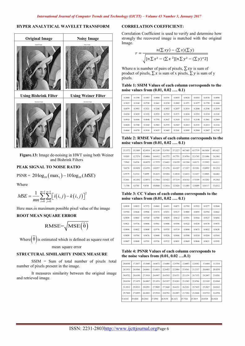
HYPER ANALYTICAL WAVELET TRANSFORM



Figure.13: Image de-noising in HWT using both Weiner and Bishrink Filters

PEAK SIGNAL TO NOISE RATIO

PSNR = 10 1 1020log max 10log ( )MSE

Where

1 1 2

0 0

1 , ,m n

i jMSE i i j k i j

mn

Here max1is maximum possible pixel value of the image

ROOT MEAN SQUARE ERROR

RMSE= MSE θ

Where θ is estimated which is defined as square root of

mean square error

STRUCTURAL SIMILARITY INDEX MEASURE

SSIM = Sum of total number of pixels /total number of pixels present in the image.

It measures similarity between the original image and retrieved image.

CORRELATION COEFFICIENT:

Correlation Coefficient is used to verify and determine how strongly the recovered image is matched with the original Image.

𝑟 =𝑛(∑ 𝑥𝑦) − (∑ 𝑥)(∑ 𝑦)

√[𝑛 ∑ 𝑥2 − (∑ 𝑥 ]2 [𝑛 ∑ 𝑦2 − (∑ 𝑦)^2]

Where n is number of pairs of pixels, ∑ 𝑥𝑦 is sum of product of pixels, ∑ 𝑥 is sum of x pixels, ∑ 𝑦 is sum of y pixels.

Table 1: SSIM Values of each column corresponds to the noise values from (0.01, 0.02 …. 0.1)

0.2000 0.1390 0.1083 0.0904 0.0791 0.0693 0.0626 0.0583 0.0538 0.0498

0.3823 0.3160 0.2720 0.2441 0.2230 0.2082 0.1971 0.1877 0.1758 0.1684

0.4479 0.3983 0.3521 0.3246 0.3052 0.2857 0.2818 0.2680 0.2546 0.2439

0.4254 0.3659 0.3193 0.2935 0.2747 0.2571 0.2434 0.2353 0.2234 0.2142

0.4910 0.4446 0.4048 0.3793 0.3647 0.3419 0.3315 0.3198 0.3061 0.2969

0.4424 0.3740 0.3242 0.2963 0.2755 0.2567 0.2413 0.2331 0.2213 0.2116

0.4866 0.4370 0.3910 0.3655 0.3445 0.3241 0.3095 0.2984 0.2867 0.2742

Table 2: RMSE Values of each column corresponds to the noise values from (0.01, 0.02 …. 0.1)

25.3372 35.1849 42.4954 48.2149 52.9785 57.2227 60.7445 63.7719 66.5456 69.1627

9.9283 12.7274 15.0084 16.8412 18.3772 19.7751 21.0784 22.1745 23.1486 24.1961

7.9943 9.4536 10.8879 11.7979 12.6683 13.6359 14.1504 14.8171 15.5992 16.4111

9.0276 10.9438 12.6359 14.0337 15.1270 16.4107 17.3227 18.3241 19.0992 20.1232

6.9579 8.2314 9.4099 10.2635 10.9204 11.8818 12.4633 13.1657 13.8805 14.6462

8.2661 10.3292 12.0872 13.3964 14.5422 15.7219 16.6162 17.5109 18.3202 19.2562

7.1750 8.5765 9.8701 10.8048 11.5014 12.5426 13.1495 13.8499 14.6117 15.4312

Table 3: CC Values of each column corresponds to the noise values from (0.01, 0.02 …. 0.1)

0.8830 0.8015 0.7373 0.6863 0.6451 0.6071 0.5782 0.5522 0.5277 0.5044

0.9784 0.9646 0.9506 0.9374 0.9251 0.9127 0.9005 0.8893 0.8784 0.8662

0.9859 0.9803 0.9740 0.9700 0.9659 0.9612 0.9591 0.9564 0.9527 0.9492

0.9821 0.9736 0.9646 0.9561 0.9488 0.9394 0.9322 0.9238 0.9170 0.9075

0.9894 0.9852 0.9808 0.9778 0.9755 0.9719 0.9698 0.9673 0.9652 0.9630

0.9850 0.9764 0.9676 0.9600 0.9528 0.9446 0.9380 0.9310 0.9244 0.9164

0.9887 0.9840 0.9791 0.9756 0.9732 0.9691 0.9669 0.9646 0.9621 0.9595

Table 4: PSNR Values of each column corresponds to the noise values from (0.01, 0.02 ….0.1)

20.0556 17.2037 15.5640 14.4672 13.6488 12.9794 12.4607 12.0382 11.6684 11.3334

28.1933 26.0360 24.6041 23.6033 22.8452 22.2084 21.6541 21.2137 20.8403 20.4559

30.0752 28.6189 27.3919 26.6947 26.0765 25.4371 25.1154 24.7155 24.2687 23.8281

29.0194 27.3475 26.0987 25.1874 24.5357 23.8283 23.3585 22.8704 22.5105 22.0569

31.2812 29.8213 28.6591 27.9049 27.3660 26.6331 26.2181 25.7419 25.2827 24.8163

29.7848 27.8495 26.4843 25.5910 24.8782 24.2007 23.7202 23.2646 22.8722 22.4394

31.0144 29.4646 28.2444 27.4584 26.9158 26.1631 25.7526 25.3019 24.8368 24.3628




lalitha

Text Box

148



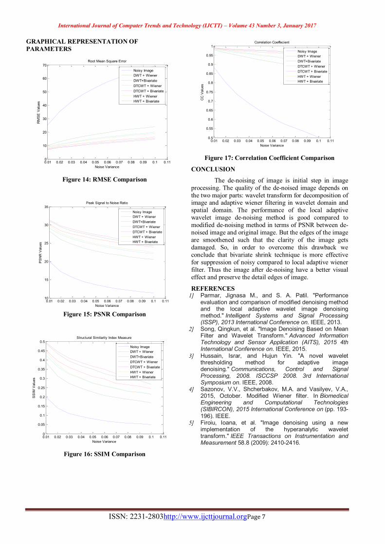
GRAPHICAL REPRESENTATION OF PARAMETERS

Figure 14: RMSE Comparison

Figure 15: PSNR Comparison

Figure 16: SSIM Comparison

Figure 17: Correlation Coefficient Comparison

CONCLUSION

The de-noising of image is initial step in image processing. The quality of the de-noised image depends on the two major parts: wavelet transform for decomposition of image and adaptive wiener filtering in wavelet domain and spatial domain. The performance of the local adaptive wavelet image de-noising method is good compared to modified de-noising method in terms of PSNR between de-noised image and original image. But the edges of the image are smoothened such that the clarity of the image gets damaged. So, in order to overcome this drawback we conclude that bivariate shrink technique is more effective for suppression of noisy compared to local adaptive wiener filter. Thus the image after de-noising have a better visual effect and preserve the detail edges of image.

REFERENCES 1] Parmar, Jignasa M., and S. A. Patil. "Performance

evaluation and comparison of modified denoising method and the local adaptive wavelet image denoising method." Intelligent Systems and Signal Processing (ISSP), 2013 International Conference on. IEEE, 2013.

2] Song, Qingkun, et al. "Image Denoising Based on Mean Filter and Wavelet Transform." Advanced Information Technology and Sensor Application (AITS), 2015 4th International Conference on. IEEE, 2015.

3] Hussain, Israr, and Hujun Yin. "A novel wavelet thresholding method for adaptive image denoising." Communications, Control and Signal Processing, 2008. ISCCSP 2008. 3rd International Symposium on. IEEE, 2008.

4] Sazonov, V.V., Shcherbakov, M.A. and Vasilyev, V.A., 2015, October. Modified Wiener filter. In Biomedical Engineering and Computational Technologies (SIBIRCON), 2015 International Conference on (pp. 193-196). IEEE.

5] Firoiu, Ioana, et al. "Image denoising using a new implementation of the hyperanalytic wavelet transform." IEEE Transactions on Instrumentation and Measurement 58.8 (2009): 2410-2416.

0.01 0.02 0.03 0.04 0.05 0.06 0.07 0.08 0.09 0.1 0.110

10

20

30

40

50

60

70

Noise Variance

RM

SE

Val

ues

Root Mean Square Error

Noisy ImageDWT + WienerDWT+BivariateDTCWT + WienerDTCWT + BivariateHWT + WienerHWT + Bivariate

0.01 0.02 0.03 0.04 0.05 0.06 0.07 0.08 0.09 0.1 0.1110

15

20

25

30

35

Noise Variance

PS

NR

Val

ues

Peak Signal to Noise Ratio


0.01 0.02 0.03 0.04 0.05 0.06 0.07 0.08 0.09 0.1 0.110

0.05

0.1

0.15

0.2

0.25

0.3

0.35

0.4

0.45

0.5

Noise Variance

SS

IM V

alue

s

Structural Similarity Index Measure


0.01 0.02 0.03 0.04 0.05 0.06 0.07 0.08 0.09 0.1 0.110.5

0.55

0.6

0.65

0.7

0.75

0.8

0.85

0.9

0.95

1

Noise Variance

CC

Val

ues

Correlation Coeffecient



lalitha

Text Box

149



6] Zhang, Huipin, Aria Nosratinia, and R. O. Wells. "Image denoising via wavelet-domain spatially adaptive FIR Wiener filtering." Acoustics, Speech, and Signal Processing, 2000. ICASSP'00. Proceedings. 2000 IEEE International Conference on. Vol. 4. IEEE, 2000.

7] Kazubek, Marian. "Wavelet domain image denoising by thresholding and Wiener filtering." IEEE Signal Processing Letters 10.11 (2003): 324-326.

8] Mohideen, S. Kother, S. Arumuga Perumal, and M. Mohamed Sathik. "Image de-noising using discrete wavelet transform." International Journal of Computer Science and Network Security 8.1 (2008): 213-216.

9] Ke, Li, Weiqi Yuan, and Yang Xiao. "An improved wiener filtering method in wavelet domain." Audio, Language and Image Processing, 2008. ICALIP 2008. International Conference on. IEEE, 2008.

10] Nafornita, C., & Isar, A. (2012, November). A complete second order statistical analysis of the Hyperanalytic Wavelet Transform. In Electronics and Telecommunica-tions (ISETC), 2012 10th International Symposium on (pp. 227-230). IEEE.

11] Firoiu, I. Complex Wavelet Transform. Application to Denoising. Diss. PhD thesis, Universitatea Politehnica, Timisoara, 2010.


lalitha

Text Box

150

complex wavelet transform based hyper analytical...

Documents