complex systems: self-organization vs chaos assumption · ↑pierre degond - complex systems:...

↑ ↓Pierre Degond - Complex systems: self-organization vs chaos assumption

1

Complex systems:

Self-organization vs chaos assumption

P. Degond

Institut de Mathematiques de Toulouse

CNRS and Universite Paul Sabatier

[email protected] (see http://sites.google.com/site/degond/)

Joint work with E. Carlen and B. Wennberg ;

numerical simulations by R. Chatelin


2Summary

1. Examples

2. Chaos property in particle systems

3. Binary particle dynamics on S1: the CLD & BDG

dynamics

4. Chaos property for CLD & BDG

5. Conclusion


3

1. Examples


4Complex system

➠ System with locally interacting agents

➟ emergence of spatio-temporal coordination

➟ patterns, structures, correlations, synchronization

➟ No leader / only local interactions


5Vicsek model [Vicsek et al, PRL 95]

R

Xk

ωk

➠ Time-discrete model:

➟ tn = n∆t

➟ k-th individual

➟ Xnk : position at tn

➟ ωnk : velocity with |ωn

k | = 1

➠ Xn+1k = Xn

k + ωnk ∆t

ωn+1k = ωn

k + noise (uniform in small angle interval)

ωnk =

Jnk

|Jnk |

, Jnk =

∑

j, |Xnj −Xn

k|≤R

ωnj

➠ Alignment to neighbours’ mean velocity plus noise


6Phase transition [Vicsek et al, PRL 95]

➠ Phase transition to disorder

➠ Order parameter

➟ α =∣

∣

∣N−1

∑

j ωj

∣

∣

∣

2

➟ N = particle number

➟ 0 ≤ α ≤ 1

➠ Measures alignment

α ∼ 1

ωkS1

S1

α ≪ 1

ωk

α ∼ 1: ω aligned α ≪ 1: ω random


7Phase transition to aligned state

➠ As noise decreases[Vicsek et al, PRL 95]

α(noise level)➠ As density increases[Vicsek et al, PRL 95]

α(N)

➠ Band formation [Chate et al]

Particle positions ρ (black) and α (red) (cross section)


8Self-organization

➠ Vicsek dynamics exhibits

➟ self-organization & emergence of coherent structures

➟ supposes the build-up of correlations between particles

➠ Kinetic and Hydrodynamic models rely on thechaos assumption

➟ When N is large, particles are statistically independent

➠ Question: are kinetic and hydrodynamic modelsrelevant for Complex Systems ?

➟ Goal: provide illustrative examples


9

2. Chaos property in particle systems


10Method

➠ Construct the Master equation

➟ Tells us the passage FN(tn) −→ FN(tn+1)

➟ where FN(v1, . . . , vN) = N-particle probability

distribution

➟ Note: FN invariant under permutations of {v1, . . . , vN}

➠ Compute the marginals

F(j)N (v1, . . . , vj) =

∫

FN dvj+1 . . . dvN

➟ Master eq. ⇒ eq. for the marginals

➟ Eqs. for the marginals not closed (BBGKY hierarchy)

➟ Marginals: fixed number of variables when N → ∞


11Binary interactions

➠ Hierarchy:

F(j)N (tn+1) = J (j)(F

(j+1)N (tn))

➠ Taking the limit N → ∞ ’simplifies’ the problem

➟ If N large, system is not influenced by the state of one

given particle

➠ Particles become independent

F (j)(v1, . . . , vj) =

j∏

k=1

F (1)(vk)

Chaos assumption


12Binary interactions (cont)

➠ Suppose at t = 0: particles are independent

F (j)(v1, . . . , vj)|t=0 =∏

F (1)(vk)|t=0

➠ If N finite: Dynamics builds up correlationsinstantaneously

➠ If N → ∞, correlations tend to 0

➟ for Hard-Sphere Dynamics [Lanford], ∃T s.t. ∀t ∈ [0, T ]

F (j)(v1, . . . , vj)|t →∏

F (1)(vk)|t as N → ∞

➟ BBGKY hierarchy ’converges’ to the Boltzmann eq.


13Related questions

➠ As N → ∞:

➟ Dynamics becomes irreversible

➟ ∃ entropy functional H which ց in time

➟ Dissipation

➟ Equilibria = states of maximal disorder

➠ For classical systems (e.g. rarefied gases)

➟ strong relation between these concepts

➠ Is this still true for self-organization processes ?

➟ will some of these concepts survive while others won’t ?


14

3. Binary particle dynamics on S1:

the CLD & BDG dynamics


15Dynamics on S1

➠ Setting

➟ N particles with velocities vk ∈ S1

➟ i.e. vk ∈ R2 with |vk| = 1

➟ Space homogeneous problem ⇒ kein x !!!

➟ All particles can interact

➠ State of the system at the n-th iterate

➟ ZN(tn) = (v1, . . . , vN)(tn) ∈ (S1)N

➟ tn = n∆t

➟ Discrete stochastic dynamics ZN(tn) −→ ZN(tn+1)


16Ex. 1: Space-homogeneous Vicsek dynamics

➠ Compute average direction v =∑

k vk / |∑

k vk|

➠ Add independent noise v′k = v wk

➟ g(z) proba on S1, symmetric g(z) = g(z∗)

➟ wk: N independent random var. drawn according to g

vvk

S1 v′k

➠ Note:

➟ Multiplicative group structure of S1

➟ Also use phases θ s.t. v = eiθ

➟ All particles interact ⇒ no reduction using marginals


17Ex 2. A ’binary’ Vicsek dynamics: BDG

➠ After [Bertin, Droz, Gregoire]

➠ Pick a pair {i, j} at random

➟ probability Pij = 2/N(N − 1)

➟ average direction: vij = (vi + vj)/|vi + vj|

➠ Add independent noise drawn according to g:

➟ v′i = vijwi v′

j = vijwj

➟ All particles but {i, j} unchanged

S1

vi

v′ivv′j

vj➠ Variant (acception-rejection)

➟ Collision performed with probability

h(viv∗j ) s.t. 0 ≤ h ≤ 1


18Ex 3. ’Choose the Leader’ (CLD)

➠ Pick an ordered pair (i, j) at random

➟ Probability Pij = 1/N(N − 1)

➠ Then, i joins j plus noise w drawn according to g

v′i = vjw

➟ All particles but i unchangedS

1

vi

v′ivj


19

4. Chaos property in BDG and CLD dynamics


20Noise scaling

➠ Outline

➟ Compute the masters eq. and the marginals

➟ Let N → ∞ while scaling noise variance appropriately

➠ Assumptions on noise distribution as N → ∞:

gN → δ(v)

Var(gN) =σ2

Ni.e. MSD(gN) = O(

1√N

)

➠ Goal: find eqs. for the marginals as N → ∞ and∆t = O( 1

N2 ) (continuous time limit)


21Master eq: methodology

➠ Take any observable φ(v1, . . . , vN)

➟ Denote ZN(tn) = (v1, . . . , vN)(tn) the state of the

system at time tn

➟ Markov transition operator

Q∗φ(v1, . . . , vN) = E{φ(ZN(tn+1)) |ZN(tn) = (v1, . . . , vN)}

➠ Denote FN(v1, . . . , vN) = N-particle proba:

E{φ(ZN(tn+1))} =

∫

φ FN(tn+1) dZ =

∫

(Q∗φ) FN(tn) dZ

➟ FN(tn+1) = QFN(tn) where Q = adjoint of Q∗


22Example: CLD

Q∗φ(v1, . . . , vN) =

1

N(N − 1)

∑

i6=j

∫

S1

φ(v1, . . . , wvj, . . . , vj, . . . , vN)g(w) dw

QFN(v1, . . . , vN) =

1

N(N − 1)

∑

i6=j

g(vjvi∗i )

∫

S1

FN(v1, . . . , wi, . . . , vN) dwi


23Example: BDG

Q∗φ(v1, . . . , vN) =2

N(N − 1)

∑

i<j

{∫

S1

h(√

viv∗j )×

×φ(v1, . . . , v′i, . . . , v

′j, . . . , vN) g(v∗

ijv′i)g(v∗

ijv′j) dv′

i dv′j

+ (1 − h(√

viv∗j ))φ(v1, . . . , vN)

}

with mid-direction vij defined by

vij = (vi + vj) / |vi + vj|


24N → ∞ in CLD

➠ Small noise limit

➟ gN → δ Var(gN) = σ2/N ∆t = O(1/N2)

➠ First marginal:

∂tf(1) − (σ2/2)∂2

θ1f (1) = 0

➠ Second marginal:

∂tf(2) − (σ2/2)∆θ1,θ2

f (2) +2f (2) = (f (1)(θ1)+ f (1)(θ2))δ(θ2 − θ1)


25Stationary states as t → ∞

➠ f (1) → f(1)eq = 1: uniform distribution on S

1

➠ f (2) → f(2)eq the unique solution of

−(σ2/2)∆θ1,θ2f + 2f = 2δ(θ2 − θ1)

➠ f(2)eq (θ1, θ2) 6= f

(1)eq (θ1) f

(1)eq (θ2)

➟ Chaos assumption violated

➠ f(2)eq peaked at θ1 = θ2

➟ coherent motion

➟ but no preferred mean direction


26Numerical simulations

➠ Experimental protocol

➟ simulations with N = 102, 103, 104 & 105 particles

➟ wait until ’stationary state’

➟ Pick one i and a pair (i, j) at random

➟ Redo the simulation M times to avoid correlations

➟ Plot histograms of θ1 and (θ1, θ2) of these M samples

➟ Compare with theoretical f(1)eq and f

(2)eq


27f(1)eq & f

(2)eq : experiments N = 10

3

σ = π

σ = π/10

σ = π/100


28f(2)eq : experiments vs theory N = 10

3

σ = π

σ = π/10

σ = π/100


29N → ∞ in BDG

➠ Small noise limit and continuous time limit

➟ gN → δ Var(gN) = σ2/N ∆t = O(1/N2)

➠ Strong bias (’grazing collisions’)

➟ hN/∫

hN → δ Var(hN/∫

hN) = τ 2/N

➠ Goal: in the limit N → ∞:

➟ Compare the relative influence of the noise σ and the

grazing bias τ


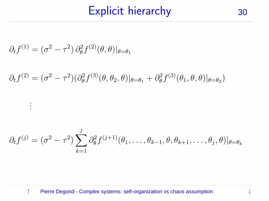
30Explicit hierarchy

∂tf(1) = (σ2 − τ 2) ∂2

θf(2)(θ, θ)|θ=θ1

∂tf(2) = (σ2 − τ 2)(∂2

θf(3)(θ, θ2, θ)|θ=θ1

+ ∂2θf

(3)(θ1, θ, θ)|θ=θ2)

...

∂tf(j) = (σ2 − τ 2)

j∑

k=1

∂2θf

(j+1)(θ1, . . . , θk−1, θ, θk+1, . . . , θj, θ)|θ=θk


31Interpretation

➠ If chaos assumption holds, f (1)(θ) satisfies

∂tf = (σ2 − τ 2) (f 2)” = 2(σ2 − τ 2) (f f ′)′

➟ nonlinear heat equation

➟ σ > τ : well-posed ; noise added wider than initial spread

➟ σ < τ : ill-posed ; noise added narrower: concentration ?

➠ BUT: Chaos assumption

does not hold

➠ Existence for hierarchy ?

➟ infinitely many stationary states


32

5. Conclusion


33Observations & Future work

➠ ’Simple’ dynamics of aggregation do not satisfychaos assumption

➟ How can kinetic theory survive this situation ?

➟ Requires rethinking of classical concepts (entroypy,

dissipation, irreversibility, equilibria, . . . )

➠ Spatialization

➟ Kinetic & fluid models

➟ application to practical systems (swarming, trail

formation, construction, . . . )

complex systems: self-organization vs chaos assumption · ↑pierre degond - complex systems:...

Documents