arX

iv:1

712.

0971

5v2

[co

nd-m

at.s

tat-

mec

h] 1

9 A

ug 2

018

Entropy balance and Information processing in bipartite and non-bipartite composite

systems

Richard E. Spinney, Joseph T. Lizier and Mikhail ProkopenkoComplex Systems Research Group, School of Civil Engineering, Faculty of Engineering and IT,

The University of Sydney, Sydney, New South Wales, Australia, 2006.(Dated: August 21, 2018)

Information dynamics is an emerging description of information processing in complex systemswhich describes systems in terms of intrinsic computation, identifying computational primitives ofinformation storage and transfer. In this paper we make a formal analogy between information dy-namics and stochastic thermodynamics which describes the thermal behaviour of small irreversiblesystems. As stochastic dynamics is increasingly being utilized to quantify the thermodynamics as-sociated with the processing of information we suggest such an analogy is instructive, highlightingthat existing thermodynamic quantities can be described solely in terms of extant information the-oretic measures related to information processing. In this contribution we construct irreversibilitymeasures in terms of these quantities and relate them to the physical entropy productions that char-acterise the behaviour of single and composite systems in stochastic thermodynamics illustratingthem with simple examples. Moreover, we can apply such a formalism to systems which do not havea bipartite structure. In particular we demonstrate that, given suitable non-bipartite processes, theheat flow in a subsystem can still be identified and one requires the present formalism to recovergeneralizations of the second law. In these systems residual irreversibility is associated with neithersubsystem and this must be included in the these generalised second laws. This opens up the possi-bility of describing all physical systems in terms of computation allowing us to propose a frameworkfor discussing the reversibility of systems traditionally out of scope of stochastic thermodynamics.

I. INTRODUCTION

In the early 1990s Evans and co-workers [1] first mea-sured the probability of “second law violations” that oc-cur in small systems. This new found ability to quantifythermodynamic quantities at scales where uncertaintiesdominate opened up a new frontier in modern thermo-dynamics leading, notably, to the now famous work re-lations of Crooks and Jarzynski [2–5]. Later a unifyingframework for general stochastic systems [6] has formedthe basis for a now indispensable tool for the study ofsmall noisy systems, named stochastic thermodynamics

[7, 8]. More recently, however, such formalisms haveimplicated information theoretic measures introduced incontexts such as the exploitation of pure order [9–13],or more generally where feedback and/or measurement,is occurring [14–25] providing powerful relationships be-tween physical quantities and information. A concertedeffort is now being levelled at utilizing such a connec-tion to understand the thermodynamics of computation[26–31].

Quite separately, however, there is an alternative view-point of physical (or otherwise) processes, which positsthat they support intrinsic computation [32, 33]. In thisview subsequent states of a dynamical process are con-sidered to have been computed from earlier ones. Inpractice, however, the confidence in the precise values ofsuch subsequent states is never perfect (arising throughinherent coarse-graining, imprecise initial conditions or,in abstract, pure noise). Given this unavoidable real-ity, the central approach becomes the quantification ofthese uncertainties in a non-parametric manner throughthe introduction of information theory. This in turn pro-

vides a natural viewpoint for the characterisation of theinformation processing supported by the dynamical pro-cess. In this view, the exact structure of physical dynam-ics give way to the phenomenological predictive capaci-ties/probabilities derived from them, from which, in turn,the structure of the information processing performed bythe system can be characterized.

Background Framing such a discussion is the conceptof generalised computation and a challenge put forwardby Langton [34, 35] in the early 1990s: how can emer-gence of computation and, in particular, the emergenceof complex spatiotemporal dynamics capable of universalcomputation, be explained in a dynamic setting. In doingso, he suggested to dissect computation into three primi-tive functions: the transmission, storage andmodification

of information. Over the last decade, this decompositionhas been formalized through an emerging field called in-formation dynamics [36–46] proving itself to be useful inrevealing or explaining generic mechanisms underlyingdynamics of distributed information processing.

A common feature in several studies which used theprimitive information-processing functions in tracing in-formation dynamics is the distributed but coherent na-ture of the underlying computation [47]. For example,the coherent behavior given by swarms of animals thatself-organize in complex large-scale spatial patterns is of-ten explained by “collective memory” [48] and “collec-tive communications” expressed via wave-like cascadesof information transfer [49]. Interestingly, the informa-tion cascades have been conjectured to correspond tolong range communications that either dynamically re-organize the swarm reducing the “fragility of mass be-haviour” [50] or propagate incorrect decisions [51].

2

It has been conjectured that information plays a dy-namic role in such a self-organization [52], and morespecifically, that distributed information-processing en-ables the groups to collectively perform computation [53–55]. These conjectures have been formalized in the con-text of information dynamics [56], verifying the hypothe-sis that the collective memory within a swarm can becaptured by active information storage, while the in-formation cascades are captured by conditional trans-

fer entropy [57, 58]. This has been further verifiedfor real biological groups, such as swarms of soldiercrabs [59], schools of zebrafish responding to a roboticanimal replica [60], pairs of bats [61], rummy-nose tetras(Hemigrammus rhodostomus) fish schools [62], and so on.

A more abstract set of examples is given by dynamicsof random Boolean networks — a canonical model forGene Regulatory Networks (GRNs) [63]. When the aver-age connectivity or activity level is varied, the dynamicsundergo a phase transition between order and chaos, andit has been shown that the information storage and in-formation transfer are maximized on either side of thecritical point: for fully-random topologies the informa-tion storage dominates the ordered phase of dynamicsand the information transfer is the primary information-processing primitive at the chaotic phase [64]. When theunderlying topology changes as well, specifically whenit undergoes an order – small-world – randomness tran-sition, the interplay between information storage andtransfer attains a balance so that the network near thesmall-world state retains a sufficient amount of storagecapability while being able to transfer information at ahigh rate [65].

Information dynamics methods have also been success-fully used for online machine learning in robotic and ar-tificial life scenarios [66–70], again allowing the designersto guide the automated learning process along specificinformation-processing primitives and fine-tune the com-putational balances, in addition to providing novel in-sights across a broad range of fields including in: canon-ical complex systems such as cellular automata [36], in-terpretation of dynamics in [43] and improved algorithmsfor machine learning [46], characterizing information pro-cessing signatures in biological signalling networks [44],non-linear time-series forecasting [71], and in computa-tional neuroscience applications in identifying neural in-formation flows from brain imaging data [45, 72, 73],inferring effective network structure [74–76], providingevidence for the predictive coding hypothesis [77] andidentifying differences in predictive information in autismspectrum disorder subjects and controls [78].

Despite these developments, the character of physi-cal entropic balances between the information-processingprimitives engaged in a distributed computation has notbeen fully elucidated. And indeed, until now the sepa-rate perspectives of stochastic thermodynamics and in-formation dynamics have not been comprehensively un-derstood in terms of each other.

As such our study has the following motivation — how

might the computational primitives described in informa-tion dynamics manifest themselves in thermodynamics?— and in what way might physical bounds or constraintsupon the system be expressed solely in terms of the com-putational primitives that the system supports? And dosuch quantities point to a dynamic generalization of thecurrent thermodynamic bounds purely in terms of infor-mation theoretic characterisations of the dynamics?

Outline In this paper, in order to answer the abovequestions, we explicitly introduce the notion of irre-versibility into the language of distributed computationand in doing so make a formal connection between infor-mation dynamics and stochastic thermodynamics, specif-ically in terms of stored and transferred information andthe bounds they place on each other.

Through the definition of an appropriate time reversed

computation, we discuss the storage and transfer of in-formation of time reversed behaviour and consequentlyidentify irreversibility measures associated with storedand transferred information. Importantly, for physicalsystems which permit identification of an unambiguousentropy production, this total entropy production is iden-tically equal to the sum of irreversibilities associated withstorage and transfer of information. This allows us toidentify contributions to the physical entropy productionsolely in terms of computational primitives.

We illustrate the behaviour of such entropy productioncontributions in a variety of increasingly broad situations.First we consider the canonical situation in stochasticthermodynamics, namely that of a system controlled byan external protocol, illustrating that the entropy pro-duction associated with information transfer to the pro-tocol is intimately related to the irreversibility in the dy-namics of that protocol, demonstrating different boundson the contributions for reversible and irreversible pro-tocol dynamics. We then apply the framework to com-posite systems, considering first bipartite systems. Weshow that our framework identifies the physical entropycontributions which allow the second law to be locallybroken for individual subsystems, for instance in the con-text of feedback, in contrast to previous approaches andresults which aim to bound such terms with informationtheoretic measures. In considering such composite sys-tems, we introduce a principle of conserved predictivecapacity, which constrains the extent to which compu-tational primitives of the total system can be associatedwith the individual subsystems. We find that such aprinciple always leads to the existence of an interactionterm understood to be a predictive capacity not uniquelyattributable to any individual subsystem. Further thisinteraction term is essential for constructing generaliza-tions of the second law in terms of stored and transferredinformation. For bipartite systems this interaction termreduces to the change in mutual information recoveringprevious results where such terms are introduced ad-hoc

in order to construct the appropriate bounds.

Moreover, because our formalism identifies contribu-tions to the entropy production using physically agnostic

3

information theoretic measures, the resultant relationsare valid where previous ones are not. Specifically, theyapply non bipartite systems where we can still associatecomputational irreversibility despite unambiguous heatflows not necessarily being well defined. Importantly,in these systems the relations from our formalism thathold for bipartite systems remain unchanged, naturallyaccounting for intrinsic correlation in the dynamics ofthe subsystems. We emphasize that systems which arephysically meaningful are not restricted to the bipartitecase, yet previously no theory of how entropy productionshould be associated with the behaviour of individualsubsystems has been provided. As such we posit thatsuch a framework is a natural approach to the phenom-ena of irreversibility, applicable to all distributed com-puting systems, from which known bounds in stochasticthermodynamics emerge where the relevant physical as-sumptions hold.

We illustrate our results on two simple models. Thefirst is a simple bipartite model allowing illustration ofboth entropy associated with storage and transfer of in-formation. The second is a non-bipartite linear model ofa feedback controller with system and controller drivenby correlated noise. Until now we are aware of no for-malism for describing this set up. We emphasize thatphysical heats are identifiable in such a system, that pre-vious generalizations of the second law with informationtheoretic terms fail in this context, but the bounds fromthe present formalism do hold for any degree of correla-tion in the dynamics.

II. INTRINSIC COMPUTATION AND

INFORMATION DYNAMICS

The outlook that intrinsic computation may be de-composed into distinct primitives naturally frames thediscussion of computation in terms of identifying pre-cise measures of information processing which informa-tion dynamics [36–46] aims to quantify.

Originally formulated in the context of distributedcomputing systems, possessing a characteristic updateinterval, in discrete time, the central object in informa-tion dynamics is the predictive capacity which quantifiesthe transformation of uncertainty in the ‘output’, somenext state in a given time series, when all previous ‘in-put’ states, all current and previous time series data, areknown. This predictive capacity, measured in bits ornats, is characterized by a mutual information, definedbetween two variables A and B taking values a ∈ A andb ∈ B respectively, as

IM (A;B) =∑

a∈Ab∈B

p(A = a,B = b) lnp(A = a,B = b)

p(A = a)p(B = b)

=

⟨

lnp(A = a,B = b)

p(A = a)p(B = b)

⟩

, (1)

such that 〈. . .〉 indicates an ensemble expectation. Specif-ically, the predictive capacity is the mutual informationbetween the complete past of the universe and the nextcomputed state of the variable in question. We charac-terise the evolution of the variable in question, X , takingvalues x ∈ X , as a time series X0:i ≡ {X0, X1, . . . , Xi},taking values x0:i ≡ {x0, x1, . . . , xi} in a space X0:i =X⊗(i+1), such that xi = x(t = i). Similarly, the restof the universe is captured by an extraneous variableY taking values in y ∈ Y which equally is character-ized as a time series Y0:i ≡ {Y0, Y1, . . . , Yi}, taking valuesy0:i ≡ {y0, y1, . . . , yi} in a space Y0:i = Y⊗(i+1). As such

we consider the predictive capacity, C{i,i+1}X , from time

t = i to t = i+ 1, for a process started at time t = 0 as

C{i,i+1}X = IM (Xi+1;X0:iY0:i)

= H(Xi+1)−H(Xi+1|X0:i, Y0:i). (2)

The superscripts indicate, explicitly, that this predictionoccurs over the interval {i, i+1}. In this sense we under-stand that it characterises the total reduction in uncer-tainty that can be achieved about the ‘computed state’,Xi+1 = xi+1, given the inputs, namely the previous val-ues of the time series, {X0:i, Y0:i} = {x0:i, y0:i}. The in-formation theoretic quantities are then built from ensem-ble probabilities p(Xi = xi) and transition probabilitiesp(Xi+1 = xi+1|X0:i = x0:i) such that

H(Xi+1) = −∑

xi+1∈Xi+1

p(Xi+1 = xi+1) ln p(Xi+1 = xi+1)

H(Xi+1|X0:i, Y0:i)

= −∑

x0:i+1∈X⊗(i+2)

y0:i∈Y⊗(i+1)

p(X0:i+1=x0:i+1, Y0:i = y0:i)

× ln p(Xi+1 = xi+1|X0;i = x0:i, Y0:i = y0:i)(3)

etc. where here and throughout we will assume time ho-mogeneity such that any and all time variation in thedynamics/transition probabilities experienced by X isparametrized through Y .The insight from information dynamics is to divide this

total predictive capacity into computationally relevantquantities in the spirit of Langton’s conception of gener-alised computation. The pertinent division is that whichseparates the predictive capacity due to the process Xand the predictive capacity over and above that of Xdue to Y . This is written

C{i,i+1}X = H(Xi+1)−H(Xi+1|X0:i)

+H(Xi+1|X0:i)−H(xi+1|X0:i, Y0:i)

= IM (Xi+1;X0:i) + IM (Xi+1;Y0:i|X0:i)

= A{i,i+1}X + T

{i,i+1}Y→X , (4)

where IM (A;B|C) = IM (A;B,C) − IM (A;C) is aconditional mutual information between A and B given

4

C. Here A{i,i+1}X is known as the active information

storage [42] and T{i,i+1}Y→X as the transfer entropy [79],

a well known non-parametric measure of predictabilityused in many areas of science, in this instance from Yto X . We denote this division of the predictive capacity,the computational signature of the process (such adivision has been explored previously, see for example[80]). The active information storage is interpreted asthe stored information in X which is utilized in makinga transition, whilst the transfer entropy is interpreted asthe transferred information from Y utilized in makinga transition in the context of the full history of X .Importantly, since both AX and TY→X can be writtenas (conditional) mutual informations they are thusrigorously non-negative.

Recent developments have stressed that these quantitiesshould be understood as expectation values of suitablespecific, pointwise or local, quantities [42, 81]. These areknown as the local active information storage ax andlocal transfer entropy ty→x where we write

A{i,i+1}X = 〈a{i,i+1}

x 〉T{i,i+1}Y→X = 〈t{i,i+1}

y→x 〉, (5)

with

a{i,i+1}x = ln

p(Xi+1 = xi+1|X0:i = x0:i)

p(Xi+1 = xi+1)

t{i,i+1}y→x = ln

p(Xi+1 = xi+1|X0:i = x0:i, Y0:i = y0:i)

p(Xi+1 = xi+1|X0:i = x0:i)(6)

which together comprise the local predictive capacity

c{i,i+1}x = a{i,i+1}

x + t{i,i+1}y→x

= lnp(Xi+1 = xi+1|X0:i = x0:i, Y0:i = y0:i)

p(Xi+1 = xi+1)(7)

with C{i,i+1}X = 〈c{i,i+1}

x 〉. In purely information theo-retic terms, such local quantities may be interpreted asthe differences in code lengths between competing mod-els of the observed behaviour in Xi+1. It is important tonote that such local values have no bound on their signand thus may be negative. Such an approach allows sig-nificance to placed on single realisations of a process, al-lowing fine characterisation of spatial temporal features,such as the identification of dynamics that are informa-tive, but especially those which are misinformative, char-acterized by negative local values. Detailed understand-ing of these individual realisations using such local quan-tities has yielded important identification and insightsinto distributed computing behaviour. This ability to at-tribute storage and transfer of information to individualrealisations is crucial to the following developments.

III. TIME REVERSED COMPUTATIONS

Modern thermodynamics makes explicit links betweenthe dynamic irreversibility of a physical process and thetotal entropy production of the universe. Indeed, this‘total entropy production’, comprising the change in in-ternal uncertainty and the heat dissipated to an environ-ment, can be, under the right circumstances, consideredequal to the log-ratio of the probability of observing the‘forward’ behaviour relative to the probability of observ-ing the ‘reverse’ behaviour, having started from an en-semble characterized by the distribution at the end of theforward process. This entails, if not the construction, theconsideration of, a suitable ‘reverse process’ with whichthe normal, forward dynamics are contrasted.We wish to give an alternative account of irreversibil-

ity in computational terms, understood in the sense ofinformation dynamics. To do so we need to attributecomputational quantities to the time reverse behaviourof the system. Accordingly, and in contrast to the re-verse process considered in stochastic thermodynamics,we define a time reversed computation through an anal-ogous time reversed predictive capacity. Such a object isdefined axiomatically, on a local, pointwise, scale, as thepredictive capacity with all constitute elements time re-versed relative to the transition being considered in thecontext of the whole process from t0 to tn, viz.

c†,{n−(i+1),n−i}x = ln

p†(Xi+1 = x†i+1|X0:i = x†0:i, Y0:i = y†0:i)

p†(Xi+1 = x†i+1),

(8)

noting that this has been defined for the transition fromtime n− i− 1 → n− i. Here we have introduced

• The time reversed transform denoted by the † sym-bol which time reverses and reflects sequences onthe interval [0, n]. This leads to the time reversed

path x†0:n, which, in the absence of odd parity vari-ables amounts to the reverse sequence of x0:n, i.e.

x†0:n = xn:0 = {xn, . . . , x0}, such that x†i = xn−i.

• The time reversed ensemble probability, appear-

ing in the denominator, defined as p†(Xi = x†i ) =

p(X†i = x†i ) = p(Xn−i = xn−i).

• The time reversed dynamics [6, 82, 83], appearingin the numerator, which in contrast accounts forany differences that occur under time reversal inthe generator of the process. This can arise dueto dependence on odd quantities with respect totime reversal (e.g. magnetic fields/torques etc.) ordifferences in evolution related to intervention inthe system, e.g. in extraneous variables Y . Unlessotherwise stated we will consider p† = p relating toautonomous, time invariant, behaviour.

We emphasize that the probability in the numerator isof the reverse trajectory as if it were evolving forward

5

in time under dynamics denoted p†. In this sense it re-mains a prediction of a hypothetical future evolution ofthe system. We emphasize that p† is not a probability as-

sociated with retrodiction i.e. not p†(X†i+1 = x†i+1|X†0:i =

x†0:i, Y†0:i = y0:i).

For brevity we subsequently drop the explicit referenceto the variables and write the probabilities solely in termsof the realized values such that we write

c{i,i+1}x = ln

p(xi+1|x0:i, y0:i)

p(xi+1)

c†,{n−i−1,n−i}x = lnp†(x†i+1|x

†0:i, y

†0:i)

p†(x†i+1)

= lnp†(xn−i−1|xn:n−i, yn:n−i)

p(xn−i−1)(9)

and so, for the transition i → i+ 1,

c†,{i,i+1}x = ln

p†(xi|xn:i+1, yn:i+1)

p(xi)(10)

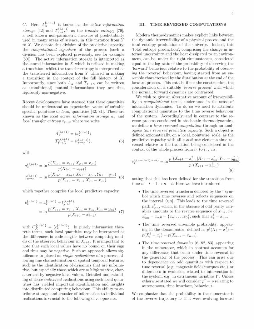
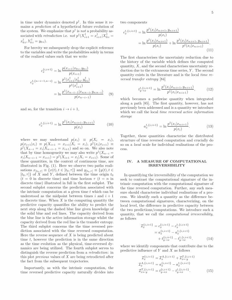
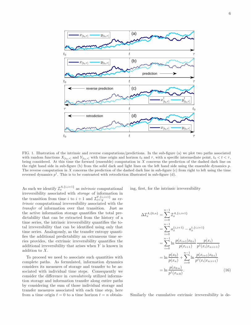
where we may understand p(xi) ≡ p(Xi = xi),p(xi+1|xi) ≡ p(Xi+1 = xi+1|Xi = xi), p†(xi|xi+1) ≡p†(Xn−i = xi|Xn−i−1 = xi+1) and so on. We also notethat by time homogeneity we may also write p†(Xn−i =xi|Xn−i−1 = xi+1) = p†(Xi+1 = xi|Xi = xi+1). Some ofthese quantities, in the context of continuous time, areillustrated in Fig. (1). Here we observe two paths reali-sations x[t0,τ ] ≡ {x(t), t ∈ [t0, τ ]} and y[t0,τ ] ≡ {y(t), t ∈[t0, τ ]} of X and Y , defined between the time origin t0(t = 0 in discrete time) and time horizon τ (t = n indiscrete time) illustrated in full in the first subplot. Thesecond subplot concerns the prediction associated withthe intrinsic computation at a given time t which can beunderstood as the midpoint between times i and i + 1in discrete time. When X is the computing quantity thepredictive capacity quantifies the ability to predict thenext step along the dashed blue line given knowledge ofthe solid blue and red lines. The capacity derived fromthe blue line is the active information storage whilst thecapacity derived from the red line is the transfer entropy.The third subplot concerns the the time reversed pre-diction associated with the time reversed computation.Here the reverse sequence of X is being predicted abouttime t, however the prediction is in the same directionas the time evolution as the physical, time-reversed dy-namics are being utilized. The fourth subplot serves todistinguish the reverse prediction from a retrodiction: inthis plot previous values of X are being retrodicted afterthe fact from the subsequent trajectories.

Importantly, as with the intrinsic computation, thetime reversed predictive capacity naturally divides into

two components

c†,{i,i+1}x = ln

p†(xi|xn:i+1, yn:i+1)

p(xi)

= lnp†(xi|xn:i+1)

p(xi)+ ln

p†(xi|xn:i+1, yn:i+1)

p†(xi|xn:i+1).

(11)

The first characterises the uncertainty reduction due tothe history of the variable which defines the computedquantity, X , and the second characterises uncertainty re-duction due to the extraneous time series, Y . The secondquantity exists in the literature and is the local time re-

versed transfer entropy [84]

t†,{i,i+1}y→x = ln

p†(xi|xn:i+1, yn:i+1)

p†(xi|xn:i+1), (12)

which becomes a pathwise quantity when integratedalong a path [85]. The first quantity, however, has notpreviously been addressed and is a quantity we introducewhich we call the local time reversed active information

storage

a†,{i,i+1}x = ln

p†(xi|xn:i+1)

p(xi). (13)

Together, these quantities characterise the distributedstructure of time reversed computation and crucially doso on a local scale for individual realisations of the pro-cess.

IV. A MEASURE OF COMPUTATIONAL

IRREVERSIBILITY

In quantifying the irreversibility of the computation weseek to contrast the computational signature of the in-trinsic computation with the computational signature ofthe time reversed computation. Further, any such mea-sure should characterise individual realisations of a pro-cess. We identify such a quantity as the difference be-tween computational signatures, characterizing, on thelocal level, the difference in predictive capacity betweenthe two predictions/computations. We introduce such aquantity, that we call the computational irreversibility,as follows

I{i,i+1}x = c{i,i+1}

x − c†,{i,i+1}x

= a{i,i+1}x − a†,{i,i+1}

x

+ t{i,i+1}y→x − t†,{i,i+1}

y→x . (14)

where we identify components that contribute due to thepredictive influence of Y and X as follows

I{i,i+1}x = IA,{i,i+1}

x + IT,{i,i+1}x←y

IA,{i,i+1}x = a{i,i+1}

x − a†,{i,i+1}x

IT,{i,i+1}x←y = t{i,i+1}

y→x − t†,{i,i+1}y→x . (15)

6

(a)

(b)

prediction

reverse prediction (c)

retrodiction (d)

FIG. 1. Illustration of the intrinsic and reverse computations/predictions. In the sub-figure (a) we plot two paths associatedwith random functions X[t0,τ ] and Y[t0,τ ] with time origin and horizon t0 and τ , with a specific intermediate point, t0 < t < τ ,being considered. At this time the forward (ensemble) computation in X concerns the prediction of the dashed dark line onthe right hand side in sub-figure (b) from the solid dark and light lines on the left hand side using the ensemble dynamics p.The reverse computation in X concerns the prediction of the dashed dark line in sub-figure (c) from right to left using the timereversed dynamics p†. This is to be contrasted with retrodiction illustrated in sub-figure (d).

As such we identify IA,{i,i+1}x as intrinsic computational

irreversibility associated with storage of information in

the transition from time i to i + 1 and IT,{i,i+1}x←y as ex-

trinsic computational irreversibility associated with thetransfer of information over that transition. Just asthe active information storage quantifies the total pre-dictability that can be extracted from the history of atime series, the intrinsic irreversibility quantifies the to-tal irreversibility that can be identified using only thattime series. Analogously, as the transfer entropy quanti-fies the additional predictability an extraneous time se-ries provides, the extrinsic irreversibility quantifies theadditional irreversibility that arises when Y is known inaddition to X .

To proceed we need to associate such quantities withcomplete paths. As formulated, information dynamicsconsiders its measures of storage and transfer to be as-sociated with individual time steps. Consequently weconsider the difference in cumulatively utilized informa-tion storage and information transfer along entire pathsby considering the sum of those individual storage andtransfer measures associated with each time step, herefrom a time origin t = 0 to a time horizon t = n obtain-

ing, first, for the intrinsic irreversibility

∆IA,{0,n}x =

n−1∑

i=0

IA,{i,i+1}x

=

n−1∑

i=0

a{i,i+1}x − a†,{i,i+1}

x

=

n−1∑

i=0

lnp(xi+1|x0:i)

p(xi+1)

p(xi)

p†(xi|xn:i+1)

= lnp(x0)

p(xn)+

n−1∑

i=0

lnp(xi+1|x0:i)

p†(xi|xn:i+1)

= lnp(x0:n)

p†(xn:0). (16)

Similarly the cumulative extrinsic irreversibility is de-

7

fined as

∆IT,{0,n}x←y =

n−1∑

i=0

IT,{i,i+1}x←y

=

n−1∑

i=0

t{i,i+1}y→x − t†,{i,i+1}

y→x

=

n−1∑

i=0

lnp(xi+1|x0:i, y0:i)

p(xi+1|x0:i)

p†(xi|xn:i+1)

p†(xi|xn:i+1, yn:i+1)

= lnp†(xn-1:0|xn)

p(x1:n|x0)

p(x1:n|x0, {y0:n-1})p†(xn-1:0|xn, {yn:1})

(17)

where we utilise notation for probabilities of completepaths as follows

p(x1:n|x0) =

n∏

i=1

p(xi|x0:i−1)

p†(xn−1:0|xn) =

n−1∏

i=0

p(xi|xn:i+1)

p(x0:n) = p(x0)p(x1:n|x0)

p†(xn:0) = p(xn)p(xn−1:0|xn)

p(x1:n|x0, {y0:n-1}) =n−1∏

i=0

p(xi+1|x0:i, y0:i)

p†(xn−1:0|xn, {yn:1}) =n−1∏

i=0

p(xi|xn:i+1, yn:i+1) (18)

with notation {} emphasizing that p(x1:n|x0, {y0:n-1}) 6=p(x1:n|x0, y0:n-1) as future values of Y are causallyblocked along evaluation of the path.

Explicitly, ∆IA,{0,n}x is the difference between the cu-

mulative use of stored information utilized in a specificpath for all computational steps from t = 0 throughto t = n and the cumulative use of stored informationin all steps of the appropriate reverse computation se-

quenced from n to 0. Analogously ∆IT,{0,n}x←y is the dif-

ference between the cumulatively transferred informationin the forward computations and the cumulatively trans-ferred information in the appropriate reverse computa-tions. Both of these are expressible as probabilities as-signed to total path realisations, i.e. x0:n etc.Importantly, these accumulated quantities along such

paths can be expressed as functionals consisting of ra-tios of the constructed path probabilities. This supportstheir existence when a limit in the discretization is takenin the approach to continuous time (thus permitting arate). In the continuum regime we are concerned withsuch quantities formulated for continuous path functionswritten xA ≡ {x(t′) : t′ ∈ A}. We construct these quan-tities by considering an interval [t0, τ ] and constructing adiscretisation running from i = 0 to i = n = (τ − t0)/∆tsuch that xi = x(t0 + i∆t) then taking ∆t → 0 such thatx0:n → x[t0,τ ], x1:n → x(t0,τ ] and so on. In this limit,

measures replace probabilities and computational signa-tures and irreversibilities become differential quantities

defined instantaneously, i.e. I{i,i+1}x → dIx(t). We con-

sequently identify the accumulated quantities with loga-rithms of Radon-Nikodym derivatives between these pathmeasures [85, 86], such that for a process running fromt = t0 to t = τ we write

∆IAx =

∫ τ

t0

dIAx (t)

= lim∆t→0

lnp(x0:n)

p†(xn:0)

= lndp[x[t0,τ ]]

dp†[x[t0,τ ]]

∆ITx←y =

∫ τ

t0

dITx←y(t)

= lim∆t→0

lnp†(xn-1:0|xn)

p(x1:n|x0)

p(x1:n|x0, {y0:n-1})p†(xn-1:0|xn, {yn:1})

= lndp†[x(τ,t0]|xτ ]

dp[x(t0,τ ]|xt0 ]

dp[x(t0,τ ]|xt0 , {y[t0,τ)}]dp†[x(τ,t0]|xτ , {y[τ,t0)}]

. (19)

For clarity, however, we utilise a deliberate abuse of no-tation rewriting measures as path probability ‘densities’such that

∫

dp[x[t0,τ ]] ≡∫

dx[t0,τ ] p[x[t0,τ ]]

=

∫

dx[t0,τ ] p[x(t0,τ ]|xt0 ]p(xt0), (20)

since this permits a more natural discussion and intuitivemanipulation when dealing with familiar objects such asmutual informations etc. without altering any of the re-sults.Before progressing we note that the intrinsic irre-

versibility associated with information storage permitsa non-negative ensemble average viz.

〈∆IAx 〉 =

∫

dx[t0,τ ] p[x[t0,τ ]] lnp[x[t0,τ ]]

p†[x[τ,t0]]≥ 0, (21)

but no bound exists for 〈∆Ix〉 or 〈∆ITx←y〉, properties

that we shall return to.

V. COMPUTATIONAL IRREVERSIBILITY IN

PHYSICAL SYSTEMS

The measures 〈∆Ix〉, 〈∆IAx 〉 and 〈∆IT

x←y〉 are verygeneral objects which quantify irreversibility for any dy-namics where the relevant probability measures can bedefined. However, in order to understand their potentialrole in, and connection with, (stochastic) thermodynam-ics we must consider their behaviour in relevant physicalsystems. This will necessarily involve a constraining ofthe nature of the systems considered. To understand the

8

relevant constraints it is instructive to give a brief ac-count of how irreversibility in physical systems can beidentified thermodynamically as entropy production.

A. Entropy production in stochastic

thermodynamics

Here we give a brief account of how entropy productioncan be understood in terms of dynamic irreversibility insystems that obey such Markovian dynamics, thus givinga brief overview of the necessary features of stochasticthermodynamics. As with all thermodynamic descrip-tions, we consider a division of the universe into a sys-tem of interest with degrees of freedom that we are awareof and an environment that we are mostly unconcernedwith and so remain ignorant of. If the system is smallenough, this ignorance of the environment renders thebehaviour of the system unpredictable, or stochastic dueto our failure to track its precise evolution. Further, ifwe have performed such a division sensibly, the environ-mental degrees of freedom will be fast in comparison tothe system allowing us to make an assumption that theinduced probabilistic dynamics are Markov, but also theassumption that the environment is at equilibrium. Insuch situations a powerful principle arises known as lo-

cal detailed balance [87–94] which relates the transitionrates that arise from exposure to the environment to theexported entropy production realized in the environment.

If we consider such a continuous time Markovian pro-cess in X on a discrete state space we may describe itsbehaviour as a sequence of instantaneous transitions. Onan interval [t0, τ ] there is a countable number of transi-tions, N , occurring at times t0 < t1 < . . . < tN < τbetween states Xt = xi, t ∈ [ti, ti+1). The dynamicsare consequently described by a set of transition rateskyx→x′ concerning a transition from x to x′ which we alsoallow to be parametrized by a smoothly varying switch-ing protocol Y . In such a scenario any such transition ismediated by the equilibrium environment and thus thelocal detailed balance relation stipulates that it is accom-panied by an entropy change in the environment, at timeti, equal to

lnkytixi−1→xi

kytixi→xi−1

= ∆Sxenv(ti) (22)

manifesting as a heat flow scaled by the environmentaltemperature when the environment is a heat bath. Bydefinition, the probability of observing such a transitionin a given time ∆t is then written p(Xt+∆t = x′|Xt =x, Yt = y) = kyx→x′∆t + O(∆t2) such that we can asso-ciate the above with transition probabilities on a short

time scale

∆Sxenv(ti)

= lnkxi−1→xi

kxi→xi−1

= lim∆t→0

lnp(Xti = xi|Xti−∆t = xi−1, Yti−∆t = yti−∆t)

p(Xti = xi−1|Xti−∆t = xi, Yti−∆t = yti).

(23)

If we have invariance in the time reversed dynamics p† =

p (i.e. kyx→x′ = ky,†x→x′) and Y is suitably smooth then wemay rewrite the above as

∆Sxenv(ti)

= lim∆t→0

lnp(Xti = xi|Xti−∆t = xi−1, Yti−∆t = yti−∆t)

p†(Xti = xi−1|Xti−∆t = xi, Yti−∆t = yti−∆t)

= lim∆t→0

lnp(xti |xti−∆t, yti−∆t)

p†(xti−∆t|xti , yti), (24)

i.e. in a form represented by the time reversed dynamicsand path sequence.In contrast, an absence of entropy production in the

environment (due to X) is associated with the times be-tween transitions, understood physically as an absence ofexchange of energy with the environment. This too canbe captured in terms of probabilities of the transition se-quence by simply observing the probability of such anabsence in the forward and time reversed dynamics to beexponentially distributed due to the Markovian dynamicsand thus given by

lnp(X(ti,ti+1) = xi|Xti = xi, {Y[ti,ti+1) = y[ti,ti+1)})p†(X[ti,ti+1) = xi|Xti = xi, {Y[ti,ti+1) = y[ti+1,ti)})

=∑

x′

∫ ti+1

ti

(ky(t),†xi→x′ − k

y(t)xi→x′)dt, (25)

which vanishes when p = p† such that kx→x′ = k†x→x′ .These contributions can be constructed in a piece-wisefashion, with waiting times interleaved between transi-tions, allowing us to consider the ratio of the conditionalprobability of the entire path x[t0,τ ] and the conditionalprobability of the entire path x[τ,t0] under the time re-versed dynamics allowing us to express the total entropyexported by the system X to the environment, along anentire path x[t0,τ ] as [6, 95]

∆Sxenv[x[t0,τ ]] =

∫ τ

t0

dSxenv(t)

= lnp[x(t0,τ ]|xt0 , {y[t0,τ)}]p†[x(τ,t0]|xτ , {y[τ,t0)}]

(26)

in this case with dSxenv(t) = δ(t−ti)∆Senv(ti). Whilst we

have described the above for a jump process, the aboverelationship is very robust, holding for all Markov sys-tems that possess a local detailed balance relationship.This can be understood by recognizing that continuous

9

dynamics, realized, for instance, as stochastic differentialequations, may be achieved through the appropriate limitof such a jump process (i.e. the Fokker Planck equationmay be derived from the master equation).Having established the form of the exported entropy

production, one of the key insights of stochastic ther-modynamics is to observe that when augmenting such aquantity with a change in pointwise (or local) Shannonentropy of the system, the sum then represents the totalentropy production, in model, of the universe [6] (con-sisting of the system and the environment) and obeysthe requisite statistical requirements to satisfy a secondlaw. Such a change in Shannon entropy, for any class ofsystem on the interval [t0, τ ] reads

∆Sxsys[x[t0,τ ]] = ln

p(xt0)

p(xτ ). (27)

If we consider such a change between the start and endof the process on x[t,τ ] this provides an initial conditionfor the path probabilities appearing in Eq. (26) such that

∆Sxtot[x[t0,τ ], y[t0,τ ]] = ∆Sx

sys[x[t0,τ ], y[t0,τ ]]

+ ∆Sxmed[x[t0,τ ], y[t0,τ ]]

= lnp[x[t0,τ ]|xt0 , {y[t0,τ)}]p(xt0)

p†[x[τ,t0]|xτ , {y[τ,t0)}]p(xτ )

= lnp[x[t0,τ ]|{y[t0,τ ]}]p†[x[τ,t0)|{y[τ,t0)}]

. (28)

It is this quantity that the second law governs, and it doesso on a statistical level. As such, assuming no feedbackbetween the system X and switching protocol Y (i.e. Ycannot depend on X), the following holds

〈∆Sxtot〉 = 〈∆Sx

sys〉+ 〈∆Sxenv〉 ≥ 0 (29)

representing the second law.Finally, however, it is important to note two key as-

sumptions. The first is the assumption of no feedback.If this is not met then the second law as written aboveneed not hold. To recover the second law in such caseseither the definition of the system must be expanded orthe result generalised. The second is the assumption ofsmoothness in Y in the preceding identification of theentropy production and its representation in terms of dy-namical probabilities. If such a criterion is not met thenotion of a heat physically dissipated by X can becomefundamentally ambiguous since the value y that entersthe local detailed balance condition is not well defined.This can occur notably if i) both X and Y are continu-ous but nowhere differentiable (as in the case of Langevinequations) and driven by correlated noise or ii) both Xand Y are discrete variables which can simultaneouslytransition. In the latter, such a situation can be avoidedby insisting that joint transitions are disallowed such thatthe dynamics of both X and Y , governed by the transition

rates ky→y′

x→x′ ({x, y} 6= {x′, y′}) may be written

ky→y′

x→x′ = (1− δx,x′)δy,y′kyx→x′ + (1 − δy,y′)δx,x′ky→y′

x

(30)

such that∑

y′ ky→y′

x→x′ = kyx→x′ and∑

x′ ky→y′

x→x′ = ky→y′

x .More broadly such a requirement specifies conditional in-dependence in the subsequent values of X and Y giventhe preceding history over small time scales, arising heresince the transition times of X and Y are not correlatedas they do not transition together, almost surely. Thisconditional independence is expressed by the following

limdt→0

p(xt+dt, yt+dt|xt, yt)

= limdt→0

p(xt+dt|xt, yt)p(yt+dt|xt, yt) (31)

which we can observe to hold for the discrete space caseby considering a transition x → x′ 6= x, y = y′, withoutloss of generality, that we have

p(Xt+dt = x′|Xt = x, Yt = y)p(Yt+dt = y|Xt = x, Yt = y)

= kyx→x′dt(1−∑

y′

ky→y′

x dt) +O(dt2)

= kyx→x′dt+O(dt2)

= p(Xt+dt = x′, Yt+dt = y|Xt = x, Yt = y) +O(dt2).(32)

In the former case with continuous paths such a con-ditional independence requirement manifests as statisti-cal independence of any noise terms between X and Y .When such a requirement is met then one may write

lnp(xt+dt|xt, yt)

p†(xt|xt+dt, yt+dt)= ln

p(xt+dt|xt, yt)

p†(xt|xt+dt, yt)+O(dt2),

(33)

identifying a term representing the local detailed balancecondition on the right hand side and recovering Eq. (26).This property of conditional independence, manifest

as independence in noise terms in continuous dynamicsand illegality of joint transitions in discrete dynamics, iscalled a bipartite property.

B. Relating computational irreversibility and

physical entropy production

Here we make an explicit connection between the mea-sures of computational irreversibility established in sec-tion IV and the thermodynamic quantities describedabove. To do so we consider, first, a system where thephysical assumptions listed above are true, namely that:i) an equilibrium environment leads to stochastic dynam-ics in a system, X , which are Markov thus leading to a lo-cal detailed balance relation and ii) that the joint dynam-ics of the system X and some extraneous parameter Y ,which may represent an external protocol or some othercoupled subsystem, are bipartite such that we observe nojoint transitions or consider independence of noise in thecontinuous limit.In this case we straightforwardly compare the contents

of Eq. (28) and Eq. (19) and and immediately recognize

10

a central observation

∆Ix = ∆Sxtot. (34)

Explicitly, the computational irreversibility reduces tothe total thermodynamic entropy production in the caseof Markovian bipartite dynamics revealing that the cen-tral measure of intrinsic computation, the predictive ca-pacity, can be seen to be an implicitly central quantityin stochastic thermodynamics. In other words, entropyproduction can be equivalently described by physical irre-versibility and equivalently by computational irreversibil-ity as measured by information dynamics.Since thermodynamic and computational irreversibil-

ity are equivalent in such a setting and the computationalirreversibility is designed around a division in storage andtransfer of information, it is instructive to translate sucha division, realized in the intrinsic and extrinsic computa-tion irreversibilities in Eq. (19), into divisions of physicalentropy production. As such we therefore explicitly write

dSxtot = dSx

storage + dSx←ytransfer (35)

where we identify dSxstorage = dIA

x as the physical entropyproduction associated with the active storage of informa-tion and dSx←y

transfer = dITx←y as the physical entropy pro-

duction associated with the transfer of information basedon the identification dSx

tot = dIx = dIAx + dIT

x←y . The

last quantity, dSx←ytransfer was used in the construction of

a measure of information theoretic time asymmetry, an‘information theoretic arrow of time’ [84]. We emphasizehere, however, that we are making a complete divisionof the entropy production associated with the computa-tional primitives, deriving from general measures of irre-versibility.Such a division is to be contrasted with other impor-

tant divisions of the total entropy production of the uni-verse, such as the usual division into the entropy changeattributed to the system and the environment [6] (or inthe language of Prigogine, the system into the internaland external productions [96])

dSxtot = dSx

sys + dSxenv (36)

or the more recent division of the total entropy pro-duction into adiabatic and non-adiabatic contributions[95, 97–100]

dSxtot = dSx

na + dSxa . (37)

All of the above divisions of the total entropy productionare based, in some sense, on how they manifest. The divi-sion in Eq. (36) characterises the location associated withthe entropy change: dSx

sys concerns the entropy changeassociated with the system whilst dSx

env concerns the en-tropy change of the environment. The division in Eq. (37)characterises the ensemble level mechanisms that lead todissipation: dSx

na concerns the entropy production associ-ated with driving & relaxation and dSx

a concerns the en-tropy production associated with steady non-equilibrium

constraints. Our division in Eq. (35) does so based onthe their manifestation of computational behaviour (stor-age and transfer), defined in terms of predictive capacity

based on the terms laid out in section II.Finally, we mention that since the total computational

irreversibility can be associated with physical entropyproduction, by assuming a heat bath at constant tem-perature β−1 (we use kB = 1 throughout), we can write

dSxstorage = dSsys + dβQx

storage

dSx←ytransfer = dβQx←y

transfer (38)

where

∆Qx = ∆Qxstorage +∆Qx←y

transfer. (39)

reminiscent of the identification of the non-adiabatic en-tropy production with the system entropy and excessheat [95, 101], and the adiabatic entropy production withthe house keeping heat [95, 102, 103]. That is we canidentify contributions to physical heat flows associatedwith storage and transfer of information.Next, we turn our attention to the behaviour of these

contributions to the total entropy production. Firstly weconsider the situation outlined above, that of Markovianbipartite dynamics before considering how they behavewhen the bipartite assumption is dropped.

VI. BIPARTITE SYSTEMS

In this section we explore the behaviour of the entropyproductions associated with the storage and transfer ofinformation in systems that are described through the dy-namics of two variablesX and Y and where the dynamicsare of these variables are both bipartite and Markov. Toreiterate, these are systems where, if jumps in the vari-ables are permitted, they cannot occur simultaneously inboth X and Y . Continuous bipartite dynamics can beconsidered by considering the limiting behaviour of suchsystems resulting in a conditional independence condi-tion.It is important to understand that such dynamics may

describe both a system comprising two components of atotal physical system in contact with a heat reservoir, ora single variable X controlled by switching protocol Y asthe dynamic assumptions in both cases are identical. Assuch in this section we first consider the contributions as-sociated with system X in the context of of a protocol Y ,before describing the joint contributions of the compositesystem.

A. Single variable and switching protocol

Here, we consider the simplest systems available forconsideration. These systems are the typical, canoni-cal, systems found in the original literature of stochastic

11

thermodynamics consisting of a single particle or objectof interest denoted the ‘system’ (which may be a compos-ite system itself), represented here by X , and a switch-ing protocol that determines the nature of the dynamicsthrough the change of a potential/nature of a heat bathetc., represented here by Y . In addition to the Markovand bipartite dynamics, and in contrast to systems weconsider subsequently, we do not permit any feedbackbetween the switching protocol and the particle. Conse-quently it follows that we may write the probability ofobserving the joint path {x[t0,τ ], y[t0,τ ]}

p[x[t0,τ ], y[t0,τ ]]

= p(xt0 , yt0)p[x(t0,τ ]|xt0 , {y[t0,τ)}]p[y(t0,τ ]|yt0 , {x[t0,τ)}]= p[x(t0,τ ]|xt0 , {y(t0,τ ]}]p[y(t0,τ ]|yt0 ]p(xt0 |yt0)p(yt0)= p[x[t0,τ ]|y[t0,τ ]]p[y[t0,τ ]], (40)

noting that here the evolution of Y is independent of X ,i.e. p[y(t0,τ ]|yt0 , {x[t0,τ)}] = p[y(t0,τ ]|yt0 ], and thus thatp[x(t0,τ ]|xt0 , {y(t0,τ ]}] = p[x(t0,τ ]|xt0 , y(t0,τ ]].

The division in Eq. (39) identifies heat flows based oninformation theoretic constructs, on the level of individ-ual behaviour, provided by the physical dynamics, butalso by the statistics of the ensemble which serves tochange the character of the predictability of the process.Explicitly this means changing the properties of the en-semble amounts to changing the amount of informationthat can be deemed to be in active storage or being trans-ferred and thus the irreversibility associated with it.

As such it is illustrative to consider different situa-tions where one observes different storage and transferbehaviour and thus different contributions to the totalentropy production. To do so under the system/protocolparadigm without feedback we consider three cases, eachwith increasing constraint.

1. Irreversible protocols

First we consider the case where the protocol is cho-sen randomly according to p[y[t0,τ ]], and not necessar-

ily reversibly, i.e. p[y[t0,τ ]] 6= p†[y[τ,t0]]. In this casewe have, in addition to 〈∆Sx

storage〉 ≥ 0 (which emergesfrom Eq. (21)) an integral fluctuation theorem regard-ing the total entropy production in X , plus a changein correlation between system and protocol over the pro-cess (captured by a change in a local mutual information,∆iM , where 〈iM 〉 = IM and iM = ln[p(x, y)/(p(x)p(y))]).

Specifically we may write

〈exp[−∆Sxstorage −∆Sx←y

transfer +∆iM ]〉 =∫

dx[t0,τ ]

∫

dy[t0,τ ]

× p[y[t0,τ ]]p[x(t0,τ ]|xt0 , {y[t0,τ)}]p(xt0 |yt0)

× p†[x(τ,t0]|xτ , {y[τ,t0)}]p(xτ )p(xt0 )p(xτ |yτ )p[x(t0,τ ]|xt0 , {y[t0,τ)}]p(xt0)p(xt0 |yt0)p(xτ )

=

∫

dy[t0,τ ] p[y[t0,τ ]]

×∫

dx[t0,τ ]p†[x(τ,t0]|xτ , {y[τ,t0)}]p(xτ |yτ )

= 1 (41)

such that we have 〈∆Sxstorage + ∆Sx←y

transfer〉 − ∆IM ≥ 0following from Jensen’s inequality. Consequently we seethat we have the bound

〈∆Sx←ytransfer〉 ≥ ∆IM − 〈∆Sx

storage〉 (42)

or rather

∆Sx −∆IM + β〈∆Qxstorage〉+ β〈∆Qx←y

transfer〉 ≥ 0 (43)

where ∆Sx = 〈∆Sxsys〉. We note that the final mu-

tual information, is not strictly necessary for the relationEq. (43) to hold, meaning that for an initially uncorre-lated system and protocol, we find

〈∆Sx←ytransfer〉 ≥ −〈∆Sx

storage〉. (44)

Since 〈∆Sxstorage〉 ≥ 0, 〈∆Sx←y

transfer〉 can be negative, butnot enough so that the total entropy production becomesnegative. This forms a central behaviour of the two con-tributions to entropy production: the intrinsic entropyproduction due to storage is non-negative, yet the extrin-sic entropy production due to transfer may take negativevalues, potentially offsetting contributions from its sur-roundings. The above result points out that even whenthe total entropy production (their sum) is non-negativethe entropy due to transfer may still be negative.

2. Reversible protocols

To see why 〈∆Sx←ytransfer〉 can take negative values, it is

instructive to consider progressively more restrictive pro-cesses. As such we consider a process where there is noirreversibility in the protocol: this can be considered tomean that the evolution of the protocol is purely diffu-sive, in both the forward and reverse processes, or ratherthat the protocol in the reverse process is guaranteed tobe the time reversed protocol of the forward process. Al-ternatively, one may simply posit that protocols are cho-sen from a distribution which is symmetric with respectto time reversal. All, however, yield the same condition,p[y[t0,τ ]] = p†[y[τ,t0]]. When such a condition holds, in

12

addition to the positivity of the storage entropy produc-tion 〈∆Sx

storage〉 ≥ 0, 〈∆Sxsys + β∆Qx

storage〉 ≥ 0 followingfrom Eq. (21), we may write,

〈exp[∆iM −∆Sx←ytransfer]〉

=

∫

dx[t0,τ ]

∫

dy[t0,τ ]

× p(xt0 |yt0)p[x(t0,τ ]|xt0 , {y[t0,τ)}]p[y[t0,τ ]]

× p(xt0)

p(xτ )

p(xτ |yτ )p(xt0 |yt0)

p[x(t0,τ ]|xt0 ]

p[x(t0,τ ]|xt0 , {y[t0,τ)}]

× p†[x(τ,t0]|xτ , {y[τ,t0)}]p†[x(τ,t0]|xτ ]

=

∫

dx[t0,τ ]

∫

dy[t0,τ ] p(xτ |yτ )p†[x(τ,t0]|xτ , {y(τ,t0]}]

× p[y[t0,τ ]]p[x[t0,τ ]]

p†[x[τ,t0]]]

=

∫

dx[t0,τ ]

∫

dy[t0,τ ] p(xτ |yτ )

× p†[x(t0,τ ]|xτ , {y[t0,τ)}]p†[y[τ,t0]]p[x[t0,τ ]]

p†[x[τ,t0]]

=

∫

dx[t0,τ ] p†[x[τ,t0]]

p[x[t0,τ ]]

p†[x[τ,t0]]

= 1 (45)

such that, again, by Jensen’s inequality,

−∆IM + 〈∆Sx←ytransfer〉 = −∆IM + 〈β∆Qx←y

transfer〉 ≥ 0.(46)

I.e. in this picture the single relation of Eq. (43) decom-poses into two distinct relations which we may write astwo Clausius-like statements for these processes, namely

∆Sx ≥ −β

∫ t

t0

〈dQxstorage〉

−∆IM ≥ −β

∫ t

t0

〈dQx←ytransfer〉. (47)

Differences in uncertainty and correlation, bound heatflows associated with storage and transfer of informa-tion respectively. I.e. both reflect heat flows that areassociated with behaviour attributable to X and its in-teraction with extrinsic variables. Crucially, however, wemust understand that it is the absence of irreversibility inthe extrinsic process has lead to the decomposition intotwo separate bounds facilitated by the stronger bound on〈∆Sx←y

transfer〉. In other words, there is no irreversibility ex-trinsic to X which the entropy due to information trans-fer need offset and thus the additional bound emerges.

3. Deterministic protocols

Finally, for completeness, we can consider the moretraditional conception of a process driven by a switch-ing protocol, namely that there is a single protocol

y[t0,τ ] =−→y , which can be reliably selected, repeatedly,

such that we have p[y[t0,τ ]] = δ(y[t0,τ ] − −→y ). This in

turn leads to p[x(t0,τ ]|xt0 ] → p[x(t0,τ ]|xt0 , {−→y }] and thus

∆Sx←ytransfer = ∆Sx←∅

transfer = 0 for all realisations. This sim-ply serves to illustrate the fact that information is onlydeemed to be in transfer when there is a non-singularensemble associated with the extrinsic behaviour, suchthat the division of entropy into stored and transferredcomponents is trivial here.In summary, we see that when there is no variation in

the extrinsic process, no transfer of information occursand thus no entropy production can be associated withtransfer of information since knowledge of the protocoladds no predictive capacity to the underlying computa-tions. When this condition is relaxed, but we assert thatthe extrinsic process is perfectly reversible, the entropydue to transfer of information behaves like an additionalphysical heat flow, leading to two distinct second laws,as it is rigorously bounded by a change in uncertainty inthe process. Finally we see that this second bound is lostwhen the dynamics of the protocol can be intrinsicallyirreversible.The mechanism by which this happens is important.

When the protocol is irreversible, on average the realizedy[t0,t] is more probable than the corresponding reverseprotocol, y[t,t0]. By definition, the forward protocol is aless surprising event in the ensemble that characterisesthe marginalized dynamics p[x(t0,t]|xt0 ] than the reverseprotocol. This indicates that the reverse protocol hasmore predictive power in the reverse process because itis rarer than the forward protocol. This in turn leads toa reduced entropy production arising from the transfer ofinformation: one gains more predictive power using Y inthe reverse process than in the forward process preciselybecause it is rarer. This property, where the entropy pro-duction due to transfer of information is (negatively) sen-sitive to the irreversibility of the extrinsic processes is afeature that underlies much of its behaviour in more com-plicated processes.Finally we note in this section we have introduced

boundary mutual information terms, required for the rel-evant integral fluctuation theorems to hold, in a seem-ingly ad-hoc and unprincipled way. Indeed similar termsappear in the literature [104]. In the next section we offera rationalization for the inclusion of such terms based ona principle of conservation of predictive capacity.

B. Bipartite systems with feedback

Next we extend the systems considered above to sys-tems where X and Y , whilst remaining bipartite, mayevolve dependently on each other such that effect feed-back. This allows one to consider models of protocols(Y ) which can respond to the system (X) or to considera joint, composite, system, {X,Y }, identifying contribu-tions to the entropy production from each.Especially relevant to the latter case is the fact that

13

we may observe the evolution on different levels of de-scription, each of which on has distinct characterisationsboth in terms of their thermodynamics and their intrinsiccomputation. So far we have only discussed the intrinsiccomputation and thermodynamics of individual subsys-tems, but to understand the role of entropy exchange interms of intrinsic computation in such systems we mustalso understand those behaviours on the level of the com-posite system.To do so we must discuss the intrinsic computation,

computational irreversibility and thus entropy produc-tion associated with the joint system. The joint systemis one with only an intrinsic component and thus has apredictive capacity equal to its information storage, ie.

cxy = axy. (48)

We now seek to relate this predictive capacity to the in-formation processing that is occurring on the level of theindividual subsystems characterized through cx and cy.To do we posit a principle that any coherent character-isation of the composite system should assign predictivecapacity to sub-components in such a way so as to con-serve the total of the joint system. To this end we write

cxy = cx + cy + cxyint (49)

where

cx = ax + ty→x

cy = ay + tx→y (50)

are the predictive capacities of the individual subsystems.We emphasize the appearance of cxyint, a new quantity,which we call the the interaction prediction. This quan-tifies the predictive power that emerges only when jointlypredicting both X and Y , i.e. the portion of the com-putational signature of the joint process which cannotbe uniquely attached to any individual sub-system andarises from this necessity of conserving predictive capac-ity. Importantly, unlike cxy, cx, cy or their constituentquantities, cxyint has, in general, no bound on its sign inexpectation except for bipartite systems where it mustbe negative. This occurs for bipartite systems since inthis case cxyint is given by the negative pointwise mutualinformation

cxyint = iM = − lnp(x, y)

p(x)p(y). (51)

Further, to relate such a decomposition to the compu-tational irreversibilities and entropy production contri-butions we must attribute an irreversibility term to thisinteraction prediction. Using the definition of time re-versed computations laid out in section III we may iden-tify an appropriate time reversed interaction prediction

cint,†xy = c†xy − c†x − c†y (52)

which analogously leads to an interaction irreversibility

dI intxy = cintxy − cint,†xy . (53)

Since in these systems we identify dIxy = dSxytot and

dIx = dSxtot, we identify the interaction irreversibility

with an interaction entropy production, dI intxy = dSxy

int.Importantly, for these bipartite structures this simplyreduces to the negative change in pointwise mutual in-formation

∆Sxyint = −∆iM

〈∆Sxyint〉 = −∆IM . (54)

This then provides a coherent framework for the inclusionof the mutual information in Eqs. (43) and (47): it isaccounting for computational irreversibility which cannotbe associated with either X or Y . Moreover, we shall seethat such a principle forms the basis of a general approachto systems where fewer assumptions about the dynamicshold.Proceeding, as mentioned, a particular benefit of the

bipartite assumption is that it explicitly allows us to es-tablish heat flows associated with each component of thesystem, since the conditional independence of the tran-sition probabilities leads to a joint local detailed balancecondition decomposing into separate contributions fromboth X and Y [15] such that we can write

∆Sxytot = ∆Sxy

int +∆Sxtot +∆Sy

tot

= −∆IM +∆Sxstorage +∆Sx←y

transfer

+∆Systorage +∆Sy←x

transfer

= −∆IM +∆Sxsys + β∆Qx

storage + β∆Qx←ytransfer

+∆Sysys + β∆Qy

storage + β∆Qy←xtransfer (55)

with the division of heat flows obeying

∆Qxy = ∆Qx +∆Qy

= ∆Qxstorage +∆Qx←y

transfer +∆Qystorage +∆Qy←x

transfer.

(56)

Importantly, however, no individual contribution, e.g.∆Sx

tot = ∆Sxstorage + ∆Sx←y

transfer, nor, even sums of con-

tributions, ∆Sxtot + ∆Sy

tot, has a bound on its sign inexpectation; in the context of multi-component systemsthe irreversibility of one component can be negative if itis commensurately offset by positive irreversibility in theremaining components. The second law applies to thetotal system (and environment), not necessarily on eachcomponent in isolation. Importantly, however, the re-maining components which offset such a reduction must

include the interaction entropy production.The precise nature of how this phenomenon manifests

has attracted much attention in terms of informationflows, having its origins in measurement and feedbacksystems, identifying minimal correlations that can be ex-ploited to reduce the entropy of a subsystem. In thiswork we take a different approach and identify the phys-

ical entropy that can be offset in different subsystems,arguing that it is the entropy production due to informa-tion transfer that can cause negative entropy productions

14

and indeed that it is the entropy production due to in-formation transfer associated with other subsystems thathave the ability to offset this reduction. The bounds thatthen arise from the these interactions then work in inter-play with the interaction entropy production.Firstly we establish that the total entropy of the entire

system is, necessarily, positive in expectation in accor-dance with the second law, formulated here as a contri-bution entirely associated with information storage andthus is rigorously non-negative by Eq. (21), i.e.

〈∆Sxytot〉 =

∫

dx[t0,τ ]

∫

dy[t0,τ ] p[x[t0,τ ], y[t0,τ ]]

× lnp[x[t0,τ ], y[t0,τ ]]

p†[x[τ,t0], y[τ,t0]]≥ 0. (57)

Next, however, we consider the following quantity

〈exp[−(∆Sxyint +∆Sx

tot +∆Sytot −∆Sx

storage]〉 =∫

dx[t0,τ ]

∫

dy[t0,τ ] p(xt0 , yt0)p[x(t0,τ ], y(t0,τ ]|xt0 , yt0 ]

× p(xτ , yτ )p†[x(τ,t0], y(τ,t0]|xτ , yτ ]

p(xt0 , yt0)p[x(t0,τ ], y(t0,τ ]|xt0 , yt0 ]

p[x[t0,τ ]]

p†[x[τ,t0]]

=

∫

dx[t0,τ ] p†[x[τ,t0]]

p[x[t0,τ ]]

p†[x[τ,t0]]

= 1, (58)

such that we have the bound

〈∆Sxytot −∆Sx

storage〉 ≥ 0 (59)

which may be considered equivalent to

〈∆Sxyint〉+ 〈∆Sx←y

transfer〉 ≥ −〈∆Sytot〉. (60)

This, along with the property 〈∆Systorage〉 ≥ 0 indicates

that if the total entropy production of subsystem Y isnegative, it arises because of negative 〈∆Sy←x

transfer〉 compo-nents that outweigh the information storage entropy, butmoreover that this negative entropy is balanced by theentropy due to transfer of information into X along withthe interaction entropy. In the bipartite systems consid-ered here, in the steady state, this may be expressed

〈∆Sx←ytransfer〉 ≥ −〈∆Sy

tot〉 (61)

since the mutual information is unchanged, demonstrat-ing explicitly how the extrinsic entropy production in Xcontrols the second law breakage in Y .Again, as with the treatment of switching protocols

without feedback, we see a direct inverse relationship be-tween the irreversibility in an extraneous time series, hereY , and the irreversibility in X that arises from informa-tion transfer from that variable. Despite the presence offeedback, the mechanism is the same as in the case of astochastic protocol. With increased irreversibility in Y ,reflected in a positive ∆Sy

tot, most sequences y[t0,τ ] arecommon trajectories and thus well reflected in the coarse

grained dynamics making them not particularly informa-tive, whilst y[τ,t0] are rare and are thus more informativeleading to negative entropy production due to informa-tion transfer. On the other hand when ∆Sy

tot is negative,sequences y[t0,τ ] are chosen that are relatively uncommon(with respect to their time reverse, y[t0,τ ], in constructionof the marginal dynamics), leading to more informativerealisations in the dynamics of Y in the forward timedirection and thus a positive entropy production due toinformation transfer.

1. Recovery and generalization of previousinformation-thermodynamic bounds

Here we relate the bounds that we have derived, basedon describing the thermodynamic entropy production asformed from information processing quantities, with pre-vious results in the literature which generally seek tosharpen or generalize the second law with informationprocessing quantities.A well known result concerning the transfer entropy

rate in the steady state found in [16, 105, 106] reads

〈∆Sxtot〉+ Tx→y ≥ 0 (62)

which may be integrated over finite times by consideringthe pathwise transfer entropy [85]

Tx→y[x[t0,t], y[t0,t]] = lnp[y(t0,t]|yt0 , {x[t0,t)}]

p[y(t0,t]|yt0 ](63)

such that

〈∆Sxtot〉+ 〈Tx→y〉 ≥ 0. (64)

Outside of the steady state an analogous expression forBayesian networks was given in [104] by consideringthe addition of a mutual information term, which afteradapting to continuous time processes yields

〈∆Sxtot〉+ 〈Tx→y〉 −∆IM ≥ 0. (65)

We emphasize, the distinction between this relation andthe analogous relation in our framework

〈∆Sxtot〉+ 〈∆Sy←x

transfer〉+ 〈∆Sxyint〉 ≥ 0, (66)

is that all terms in the latter are understood as compo-nents of the total entropy production of the compositesystem by considering the decomposition of the observedirreversibilities along computational lines. In this way,〈∆Sxy

int〉 = −∆IM is not an ad-hoc introduction to sat-isfy the bound, but the irreversibility associated with thejoint prediction/computation in the system which mustbe accounted for. In contrast 〈∆Sy←x

transfer〉 6= 〈Tx→y〉, withthe former identified as a component of the entropy pro-duction in Y whilst the latter is a pure information term.However, our formalism can be seen to reduce to theabove if a specific choice of reverse process is considered,

15

common to the original literature on feedback protocols[21], whereby the reverse process forces the extraneousvariable, e.g. Y , to exactly retrace the path it traced inthe forward realisation, independently of X such that thereverse dynamics are distinct from the forward dynam-ics, i.e. p 6= p†. This has the specific result of settingp†[y[τ,t0], {x[τ,t0]}] = p[y[t0,τ ]] = p†[y[τ,t0]], precisely re-turning 〈∆Sy←x

transfer〉 = 〈Tx→y〉.This may give some insight into the thermodynamic

meaning, if any, of the bare transfer entropy as it isequal to the irreversibility 〈∆IT

y←x〉 analogous to the

the entropy production 〈∆Sy←xtransfer〉 in the case of non-

autonomous feedback. I.e. the transfer entropy is alimit case of 〈∆Sy←x

transfer〉 when Y has no direct ener-getic, or thermal, interpretation as in the case of a non-autonomous feedback controller.There is no general bound characterizing the relation-

ship between 〈∆Sy←xtransfer〉 and 〈Tx→y〉, with the former in

certain situations being larger or smaller than the trans-fer entropy depending on the nature of the dynamics andthe reverse behaviour. However, their equality in the caseof non-autonomous protocols, where it is relevant, allowsconfirmation of the bound in cases where 〈Tx→y〉 is com-putable, but 〈∆Sy←x

transfer〉 is not, which we shall find ofuse when we illustrate the generalised application of ourresults in a non-bipartite system consisting of a thermo-dynamic system of interest and a feedback controller.

VII. BEYOND THE BIPARTITE ASSUMPTION

In this section we apply our formalism to systemswhich do not possess the bipartite structure consideredthus far. Whilst the thermodynamics and entropy pro-duction of such systems may, at least in the case of dis-crete state spaces, be treated as a whole using conven-tional stochastic thermodynamics, treatment of the en-tropy production associated with their individual com-ponents ordinarily cannot. As discussed, this inabilityarises because under such dynamics the heat exportedto the environment does not divide into componentsthat can be exclusively associated with each sub-system.Rather, at least in some sense, there must be a compo-nent of the heat flow which is shared between the sub-systems. When considering only discrete space, contin-uous time systems such as those described as a masterequation it might seem natural to categorize such heatflows based on the nature of the transition, with a sharedheat flow being associated with those not permitted inbipartite systems, namely joint transitions. However, ineffect, this is merely categorizing distinct transitions asbipartite (individual) or non-bipartite (joint) and leavesfundamental questions unanswered. For instance, if alltransitions are joint transitions one would conclude thatall heat flow should be identified as belonging to the jointsystem. However, one may still track only the probabilis-tic behaviour of X in the context of Y and seek to char-acterise its irreversibility. Is this irreversibility related

to the irreversibility of the joint system or that of sub-system Y ? What if only the energetics of one sub-systemcan be defined if the other corresponds to a non-thermalprocess such as a feedback controller? These questionsgo entirely unanswered if the formalism simply assignsall irreversibility to the composite system. Furthermore,in the limit of continuous dynamics the bipartite condi-tion interpreted as non-coincident transitions is no longerapplicable with such a property resulting in conditionalindependence in the dynamics. In these systems both Xand Y simultaneously fluctuate on all timescales and sothe identification of heat flows is generally non-trivial,but not necessarily ill defined. For instance, as we shallexplore later, such continuous, non-bipartite, systems, ifrepresenting a physical system and correlated feedbackcontroller, the heat dissipated by the physical system canbe captured by the computational irreversibility.It is in answering these questions that we propose our

formalism has particular merit since, because it is basedon information theory, it is agnostic to the precise na-ture of the physical dynamics which are leading to theprobability distributions, yet is consistent with conven-tional stochastic thermodynamics where heat flows canbe identified as per the previous section.Explicitly we concern ourselves with systems where the

relation in Eq. (31) does not hold, i.e.

limdt→0

p(xt+dt, yt+dt|xt, yt)

6= limdt→0

p(xt+dt|xt, yt)p(yt+dt|xt, yt). (67)

To proceed, however, we take precisely the same course ofaction as before, establishing the interaction irreversibil-ity based on a principle of conservation of predictive ca-pacity according to Eq. (49), which must hold indepen-dently of the physical energetics of the system or whetherthey are identifiable. This is given by

∆I intxy = −∆IM

+ lnp[x(t0,τ ], y(t0,τ ]|xt0 , yt0 ]

p†[x(τ,t0], y(τ,t0]|xt, yt]

+ lnp†[x(τ,t0]|xt, {y[τ,t0)}]p†[y(τ,t0]|yt, {x[τ,t0)}]p[x(t0,τ ]|xt0 , {y[t0,τ)}]p[y(t0,τ ]|yt0 , {x[t0,τ)}]

= −∆IM + β∆Qxyint. (68)

Explicitly, the interaction irreversibility is comprised ofa change in mutual information which appeared in thebipartite description and a heat contribution that didnot appear. Again, this heat is not identified by jointtransitions in the composite system, but rather by theirreversibility which cannot be observed in the individ-ual subsystems. At this point we remain agnostic as towhether ∆Sx

tot has a precise meaning in these circum-stances (though we shall argue that it can in a subsequentexample) and so strictly we may deal with the compu-tation irreversibilities ∆Ix = ∆IA

x + ∆ITx←y . However,

the total entropy production of the composite system is

16

well defined and so we may still identify the contribu-tions to this composite entropy production in terms ofstorage and transfer, i.e. ∆Ix = ∆Sx

storage + ∆Sx←ytransfer

and ∆Ixyint = ∆Sxy

int, such that

∆Sxytot = ∆Ix +∆Iy +∆I int

xy

= ∆Sxstorage +∆Sy

storage

+∆Sx←ytransfer +∆Sy←x

transfer +∆Sxyint

= ∆Sxsys + β∆Qx

storage +∆Sysys + β∆Qy

storage

+ β∆Qx←ytransfer + β∆Qy←x

transfer −∆IM + β∆Qxyint(69)

such that

∆Qxy = ∆Qxstorage +∆Qy

storage +∆Qx←ytransfer +∆Qy←x

transfer

+∆Qxyint. (70)

At this point we reiterate, these are divisions of the totalheat which is well defined, but due to the lack of bipar-tite dynamics cannot necessarily associate ∆Qx

storage +

∆Qx←ytransfer = ∆Qx as we could in the previous section.

Importantly, however, these entropy productions fol-low exactly the same relationships as for the bipartitecase, by construction, with the same integral fluctuationtheorems holding, namely,

〈exp[−(∆Sxyint +∆Sx

storage +∆Sx←ytransfer +∆Sy←x

transfer)]〉 = 1

(71)

again such that

〈∆Sxyint〉+ 〈∆Sy←x

transfer〉≥ −〈∆Sx

storage〉 − 〈∆Sx←ytransfer〉 = −〈∆Ix〉, (72)

as before, lending weight to the generality of the proposedmeasures of irreversibility.Moreover, the above bound also holds when ∆Sy←x

transferis replaced by the bare pathwise transfer entropy Tx→y,as in the bipartite case, allowing us to write

〈∆Ix〉+ 〈∆I intxy 〉 ≥ −〈Tx→y〉 (73)

or rather

〈∆Ixy〉 − 〈∆Iy〉 ≥ −〈Tx→y〉 (74)

which may equivalently be expressed in the rate form〈∆Ix〉 + 〈∆I int

xy 〉 ≥ −Tx→y. This is a central result andcan be seen to generalize the well known information-thermodynamic bound 〈∆Sx

tot〉 ≥ −Tx→y and 〈∆Sxtot〉 ≥

∆IM − Tx→y explored in depth in several other works[16, 104–107] to the case of non-bipartite dynamics. Ex-

plicitly, when bipartite dynamics are employed ∆Ix re-duces to ∆Sx

tot and ∆I intxy reduces to ∆IM which then

vanishes in the steady state. It is important to note thatin both regimes the transfer entropy Tx→y bounds theirreversibility associated with the subsystem X and theirreversibility associated with its interaction with Y .

It is interesting to consider what physical systemsmight be described by such dynamics that do not permitbipartite form. Two major examples can be considered.The first is when the whole system is well defined ther-modynamically, with defined heat flows and dissipation,but has interacting parts that evolve in such a way that itcannot be traditionally decomposed any further. Alter-natively when considering autonomous measurement andfeedback one can imagine a feedback mechanism whichdoes not meet the bipartite assumption. In both caseseither the total heat of the composite system or the theheat flow in system being monitored should still be iden-tifiable. However, currently no formalism exists for char-acterizing any such division of this total heat or for char-acterizing the feedback performance in these situations.A particular case will be treated in the next section.

VIII. EXAMPLES

A. Minimal bipartite model

Here we illustrate some of the behaviour of the en-tropy production contributions with a simple model.This model consists of two subsystems interacting witha bipartite structure. The first subsystem, X , is com-prised of three states x ∈ X = {A,B1, B2}, whilstthe second subsystem, Y , is comprised of two states,y ∈ Y = {1, 2} such that there are 6 effective globalstates {x, y} ∈ X ⊗ Y. The bipartite structure insistsupon strict conditional independence in the updating ofthese subsystems, which, in continuous time, means thatthere are no instantaneous joint transitions in both Xand Y with probability 1.

The structure is an elaboration on the minimal modelintroduced in [106], but with an additional state in sub-system X . Further, we insist upon a particular transitionrate structure which entails the transition rates govern-ing subsystem Y only being dependent on whether X isin state A or the collection of states B = {B1, B2}, suchthat it cannot distinguish between states B1 and B2 thatcomprise B. This structure is illustrated in Fig. (2) alongwith specific transition rates, specified up to the tran-sition rates between the sub-states B1 and B2. Othertransitions are parametrized by the dimensionless con-stants {rx, ry} ∈ [−1, 1]⊗ [−1, 1] and timescale parame-ters γx > 0, γy > 0.

This structure allows us to separate the mechanismsthat pertain to irreversibility associated with storage andtransfer of information. This is because the transitionsbetween B1 and B2 can introduce irreversibility indepen-dently of Y , whilst the transitions between the pairs A,B and 1, 2 explicitly interact with each other, but do notintroduce any net steady current into either subsystemwhen viewed in isolation.

To this end we consider a parameterization of the tran-

17

sition rates κB1↔B2y as follows

κB1→B2y = γxk

+, ∀y ∈ {1, 2}κB2→B1y = γxk

−, ∀y ∈ {1, 2} (75)

where k+ and k− are arbitrary constants in (0, 1). Con-sidering the steady state and solving the master equationby standard methods then yields

〈∆Sxstorage〉 =

γx(rx + ry − 2rxry)(k+ − k−) ln[k+/k−]

3 ((k+ + k−) + (rx + ry − 2rxry))

+O(a)

〈∆Sx←ytransfer〉 =

4

3γx(rx − ry) ln

[1− rxrx

]

+O(a)

〈∆Sy←xtransfer〉 =

4

3γx(ry − rx) ln

[1− ryry

]

+O(a)

〈∆Systorage〉 = 0 (76)

where a = γx/γy such that we have effected a separa-tion of timescales in order to avoid the difficulty associ-ated with calculation of generally non-Markovian objects.If a further separation of timescales exists, κB1→B2

y +

κB2→B1y = γ′x ≪ γx then the storage entropy reduces to

〈∆Sxstorage〉 = (1/3)γ′x(k

+ − k−) ln[k+/k−] + O(γ′x/γx).The results in Eqs. (76) are illustrated in Fig. (3). Im-portantly we see that as we vary the feedback coef-ficient ry controlling subsystem Y the entropy due totransfer in each system is offsetting the other, with theentropy production associated with storage only vary-ing weakly based on changes in the stationary solutionto the master equation. Indeed, since in this exam-ple we have 〈∆Sy

storage〉 = 0, a stronger bound than

Eq. (59) holds, with 〈∆Sx←ytransfer + ∆Sy←x

transfer〉 ≥ 0 hold-

ing completely independently of 〈∆Sxstorage〉 in addition

to 〈∆Sxtot + ∆Sy←x

transfer〉 ≥ 0. Moreover, if we considerrx and ry to be fixed, varying only the thermodynamicforce causing asymmetry in the B1 ↔ B2 transition, wesee total independence of in the entropy productions dueto transfer as the asymmetric transitions are not impli-cated in the feedback between the two systems. Indeedwe see that the entropy production due to storage in thisexample manifests exclusively due to stationary currentwhich can only arise when k+ and k− are unequal ex-plaining the behaviour with varying k+.

B. Computational and physical irreversibility in

non-bipartite autonomous feedback systems

Generally, there are many systems that do not obeythe bipartite assumption. These range from compositesystems which permit joint transitions between differentelements, composite systems where the subsystems ex-perience thermal (or other) noise sources that cannot be

reliably idealised as being independent through to sys-tems traditionally out of scope thermodynamics. How-ever, an investigation of their irreversibility may yet yieldanalogous bounds important to their behaviour.In this section, however, we consider a particular ex-

ample, that is a system designed to model autonomousfeedback by a controller, Y , on a physical system of in-terest X . A minimal mathematical model that achievesthis is a pair of coupled Ornstein Uhlenbeck processesdescribed by the stochastic differential equations

dx = Axdt+Bydt+ VxdWx

dy = Cxdt+Dydt+ VydWy, (77)

where dWx and dWy represent thermal noise and theinherent error in the measurement process respectively.Normally these two noise sources are deemed to bestatistically independent resulting in bipartite dynam-ics, the behaviour of which has been previously studied[16, 105, 108]. However, we can quite easily posit that thenoise sources are correlated for any number of plausiblephysical reasons, for example noise in the measurementapparatus may be arising, in part, from the same ther-mal source such that the measurement suffers from noisecontamination. In this case we have 〈dWxdWy〉 = ρdtwhere ρ ∈ [−1, 1] characterises the noise correlation suchthat for ρ = 1 the noise experienced by each of X and Yare identical.This system is governed by a Fokker-Planck equation

of the form

∂tp(x, y, t) = −∇ · (Jx, Jy)

Jx = (Ax +By)p(x, y)− V 2x

2

∂p(x, y)

∂x

− ρVxVy

2

∂p(x, y)

∂y

Jy = (Cx +Dy)p(x, y)−V 2y

2

∂p(x, y)

∂y

− ρVxVy

2

∂p(x, y)

∂x(78)

which has a Gaussian steady state given in Appendix B.A well known bound that arises in information ther-

modynamics is [16, 105, 106], as usually stated in thesteady state,

dβ〈∆Qx〉dt

+ Tx→y ≥ 0 (79)

where Tx→y is transfer entropy rate. We emphasize, withcorrelated noise this relation does not hold.

1. Identification of information and heat flows

Whilst the framework outlined in section VII describeshow to divide entropy productions along computational

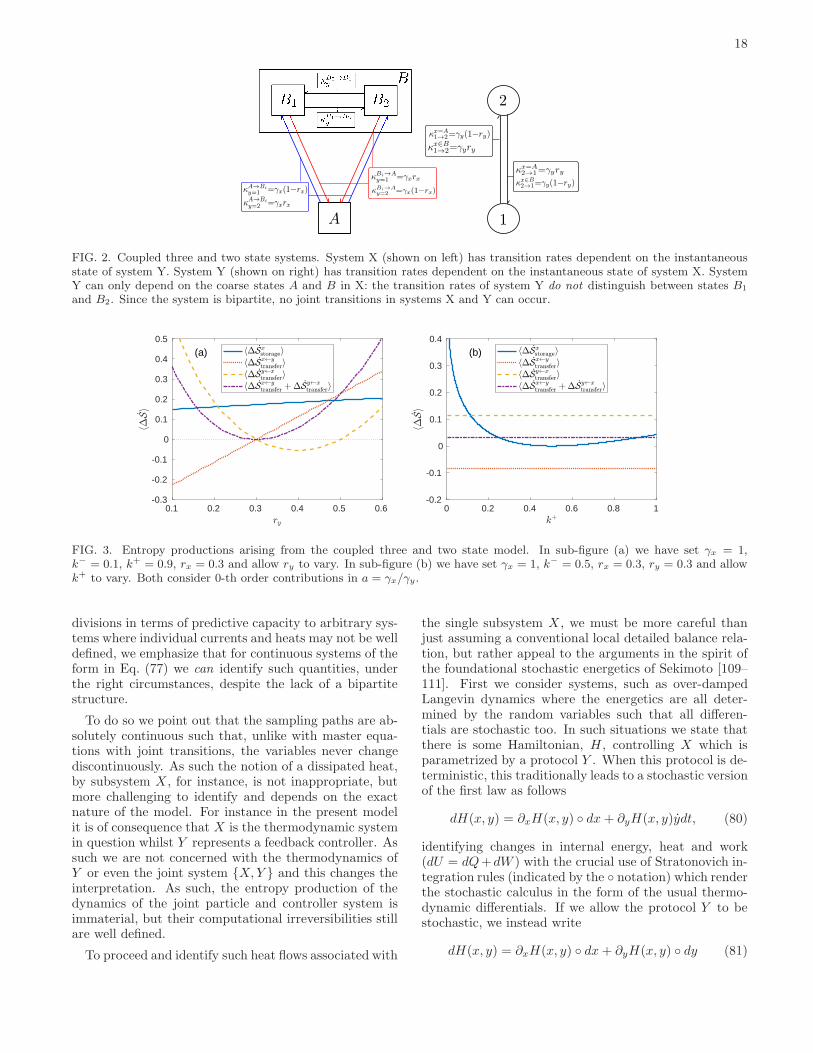
18

FIG. 2. Coupled three and two state systems. System X (shown on left) has transition rates dependent on the instantaneousstate of system Y. System Y (shown on right) has transition rates dependent on the instantaneous state of system X. SystemY can only depend on the coarse states A and B in X: the transition rates of system Y do not distinguish between states B1

and B2. Since the system is bipartite, no joint transitions in systems X and Y can occur.

0.1 0.2 0.3 0.4 0.5 0.6-0.3

-0.2

-0.1

0

0.1

0.2

0.3

0.4

0.5

(a)

0 0.2 0.4 0.6 0.8 1-0.2

-0.1

0

0.1

0.2

0.3

0.4

(b)

FIG. 3. Entropy productions arising from the coupled three and two state model. In sub-figure (a) we have set γx = 1,k− = 0.1, k+ = 0.9, rx = 0.3 and allow ry to vary. In sub-figure (b) we have set γx = 1, k− = 0.5, rx = 0.3, ry = 0.3 and allowk+ to vary. Both consider 0-th order contributions in a = γx/γy.

divisions in terms of predictive capacity to arbitrary sys-tems where individual currents and heats may not be welldefined, we emphasize that for continuous systems of theform in Eq. (77) we can identify such quantities, underthe right circumstances, despite the lack of a bipartitestructure.

To do so we point out that the sampling paths are ab-solutely continuous such that, unlike with master equa-tions with joint transitions, the variables never changediscontinuously. As such the notion of a dissipated heat,by subsystem X , for instance, is not inappropriate, butmore challenging to identify and depends on the exactnature of the model. For instance in the present modelit is of consequence that X is the thermodynamic systemin question whilst Y represents a feedback controller. Assuch we are not concerned with the thermodynamics ofY or even the joint system {X,Y } and this changes theinterpretation. As such, the entropy production of thedynamics of the joint particle and controller system isimmaterial, but their computational irreversibilities stillare well defined.

To proceed and identify such heat flows associated with

the single subsystem X , we must be more careful thanjust assuming a conventional local detailed balance rela-tion, but rather appeal to the arguments in the spirit ofthe foundational stochastic energetics of Sekimoto [109–111]. First we consider systems, such as over-dampedLangevin dynamics where the energetics are all deter-mined by the random variables such that all differen-tials are stochastic too. In such situations we state thatthere is some Hamiltonian, H , controlling X which isparametrized by a protocol Y . When this protocol is de-terministic, this traditionally leads to a stochastic versionof the first law as follows

dH(x, y) = ∂xH(x, y) ◦ dx + ∂yH(x, y)ydt, (80)

identifying changes in internal energy, heat and work(dU = dQ+dW ) with the crucial use of Stratonovich in-tegration rules (indicated by the ◦ notation) which renderthe stochastic calculus in the form of the usual thermo-dynamic differentials. If we allow the protocol Y to bestochastic, we instead write

dH(x, y) = ∂xH(x, y) ◦ dx+ ∂yH(x, y) ◦ dy (81)

19

with the division of internal energy into heat and workoperating in exactly the same way. Moreover, Eq. (81)remains unchanged under correlated noise such that theheat and work contributions are still identifiable wherewe note that Stratonovich integration includes correla-tion terms in the non-bipartite case such that

f(x, y) ◦ dx = f(x, y)dx+V 2x

2

∂f(x, y)

∂xdt

+ρVxVy

2

∂f(x, y)

∂ydt (82)

where absence of the ◦ notation indicates the non-anticipating Ito integral. Under this interpretation wemight posit some over-damped dynamics such that X isa spatial coordinate, Vx =

√

2kBT/mγ and Ax + By =−(mγ)−1∂xHx(x, y) such that we have a HamiltonianHx(x, y) = −mγ((A+B)x2−B(x−y)2), i.e. a harmonictrap with a protocol controlling an additional harmonicterm. Importantly, in this system the computational ir-reversibility reflects the ratio of heat flow to the environ-ment to the environmental temperature, β∂xH(x, y)◦dx,such that ∆Ix = ∆Sx

storage+∆Sx←ytransfer = ∆Sx

sys+β∆Qx.On the other hand, in situations where the system con-

tains degrees of freedom which are not stochastic, but ap-pear in the Hamiltonian an additional correlation termappears in the computational irreversibility which has nothermodynamic analog. In these cases we must insteadidentify

∆Ix = ∆Sxsys + β∆Qx +∆Sx

corr (83)

where ∆Sxcorr is the difference in heat flows between that

which can be physically associated with X and thatwhich is associated with the irreversibility of X such that

dSxcorr = βdQx

corr = lnp†(xt|xt+dt, yt+dt)

p†(xt|xt+dt, yt). (84)

This situation arises due to parity differences in thevariables separating the current into reversible and ir-reversible components [112]. Consequently differentialforms for the environmental entropy production intro-duce a correlation term that would arise from stochasticintegration of the reversible current, but does not emergein the stochastic energetics since the energetic term arisesfrom integration with respect to some deterministic vari-able (i.e. one not subject to noise), e.g. the particle po-sition in a full under-damped Langevin description. Weemphasize, in such situations great care must be takento identify the exact nature of the dynamics and anyHamiltonian, if any, they are emerging from in order tocorrectly identify irreversible and reversible currents. Wealso mention that correlated noise must be treated care-fully in systems with odd variables where the noise itselfmay be required to transform under time reversal [113].For the remainder we shall consider the case of the for-

mer, where, in the steady state we consider 〈∆Sxstorage +

∆Sx←ytransfer〉 = β〈∆Qx〉, for brevity, but acknowledge the

possibility of this additional step in the identification ofthe environmental entropy production in different mod-els.Returning to the model in question we reiterate that

the naive application of the traditional information theo-retic bound on the computational/physical irreversibilitydoes not hold, i.e.

d〈∆Sxstorage〉dt

+d〈∆Sx←y

transfer〉dt

+ Tx→y � 0. (85)

Instead, in order to find reliable bounds we must turn toour formulation in terms of computational irreversibili-ties which accounts for the interaction entropy produc-tion. As such the appropriate bound is

d〈∆Sxtot〉

dt+

d〈∆I intxy 〉

dt+

d〈∆Sy←xtransfer〉dt

≥ 0 (86)

or

d〈∆Sxtot〉

dt+

d〈∆I intxy 〉

dt+ Tx→y ≥ 0. (87)

to account for the non-bipartite dynamics. We note theinclusion of the more general ∆I int

xy rather that ∆Sxyint

in the bound because, as discussed, whilst the computa-tional irreversibility of the joint particle/controller sys-tem is well defined, it is not related to an entropy pro-duction in this case.For the present example we are in a position to illus-

trate such a bound mathematically. In the steady state,the transfer entropy of this system permits an analyticalsolution, adapted from [16] (see also [114]), derived inappendix C,

Tx→y =1

2

(√

A2 − 2ρACVx

Vy+ C2

V 2x

V 2y

−√A2 − ρC

Vx

Vy

)

.

(88)

Meanwhile, the rate of computational irreversibility in Xin the steady state, here equal to the entropy productionrate, is given by

d〈∆Sxtot〉

dt=

B(CV 2x − Vy(ρ(A−D)Vx +BVy))

(A+D)V 2x

. (89)

For completeness we also point out that for this systemwe have

d〈∆Sxcorr〉

dt=

ρBVy

Vx. (90)

We may then in turn compute the interaction entropyrate, again in the steady state, which due to a slightlycumbersome form we report in appendix B. Together,these objects obey the bound in Eq. (87). These are il-lustrated in Fig. (4) where they are contrasted with theusual bipartite relation and, again for completeness, thebound with ∆Sx

tot replaced with ∆Sxtot −∆Scorr

x . Impor-tantly we see that the previous conception of the gener-alised second law in such a system fails for some value ofcorrelation ρ, holding for ρ = 0 where the system reducesto the usual bipartite model.

20

-1 -0.5 0 0.5 1-0.5

0

0.5

1

1.5

FIG. 4. Coupled linear feedback model. We set A = −2, D = −4, B = C = 1, Vx = 2, Vy = 3/2 and allow the correlation, ρ,to vary.

IX. DISCUSSION AND CONCLUSIONS

In this paper we have considered computations de-scribed in the framework of information dynamics. Us-ing such a framework we have defined appropriate timereversed computations and shown that the difference be-tween each results in a measure of irreversibility that canbe divided into computationally meaningful quantities:those that relate to the storage and transfer of informa-tion. By applying such a framework to physical systemswe have shown that such a measure of computational ir-reversibility maps onto the total entropy production instochastic thermodynamics revealing that not only caninformation processing lead to bounds on thermodynam-ics, as previously conceptualized, but that thermodynam-ics may be entirely described in terms of information pro-cessing.Moreover, the framework based on information dynam-

ics that we have presented is not restricted to the bipar-tite and multipartite systems previously considered instochastic thermodynamics. By dividing irreversibilityalong the lines of computational primitives, componentsof the total physical heat can be associated with irre-

versibility even when the physical heats exported by thesub-systems are ambiguous. Further we have shown thatthese irreversibilities based on storage and transfer arecritically implicated in the resulting bounds that gener-alize the second law both when a bipartite assumptionholds and when it does not. In both cases the boundsare achieved by correctly accounting for an interactionentropy production which is always involved in its for-mulation and derived from a principle of conserved pre-dictive capacity. Further, through the use of continuousdynamics with feedback and correlated noise we have pre-sented a system where the physical heat exported by asubsystem is identifiable despite being governed by non-bipartite dynamics. Importantly, for this system, we havedemonstrated that previous generalizations of the secondlaw which account for feedback fail, whilst the boundarising from this formalism holds.

We hope that such a framework will allow discussionof irreversibility in systems where identification of indi-vidual heat flows are problematic and, moreover, allowdiscussion of thermodynamic processes in terms of dis-tributed computation.

Appendix A: Generalised computations

Whilst not strictly necessary for the development of irreversibility measures, the intrinsic (forward) and timereversed computations can be unified through the notion of a generalised intrinsic computation. To define such anobject we appreciate that the basic structure of the intrinsic computation is the reduction in uncertainty of the nextstep in a time series, relative to an ensemble prior using the past sequence of events and a transition probability. Andit is this notion that we seem to generalize based on the recognition of its structure in terms of uncertainties. Firstwe allow the prediction, or reduction of uncertainty, of some arbitrary event ε, taking values in some space E , ratherthan merely the next step in the time series. This event must be computable with a sequence of states of variable X ,

that we write−→X , taking values −→x ∈ −→X . Consequently we write ε = f(−→x ) such that f :

−→X → E . We then wish to

21

discuss the realisations of X that lead to the event ε such that we consider the pre-image of ε

f−1(ε) = {−→x ∈ −→X |f(−→x ) = ε}. (A1)

Associated with this set of realisations −→x we have a prior distribution on−→X , denoted, Q(−→x ∈ A), which represents

our prior uncertainty in sets of −→x . As such, the prior uncertainty in the specific event ε corresponds to A = f−1(ε),i.e. Q(−→x ∈ f−1(ε)).Finally we consider an inference scheme that provides a posterior, which quantifies uncertainty in ε in the presence

of some evidence−→Z taking values −→z ∈ −→Z , where, like

−→X ,

−→Z consists of some time series. This inference scheme is

represented with a probability measure P(−→x ∈ A|−→z ) where A ⊆ −→X where, again, the set corresponding to the eventε is A = f−1(ε), such that the uncertainty under inference scheme P and evidence −→z is P(−→x ∈ f−1(ε)|−→z ).Specifying all such quantities defines a tuple C = {−→X, f,

−→Z ,P,Q} that entirely characterises the local computational

signature of this generalised computation through the consideration of

cC = lndP(−→x ∈ f−1(ε)|−→z )dQ(−→x ∈ f−1(ε))

. (A2)

In these terms we can identify the (forward) intrinsic computation, at time i, as being characterized by the tuple

C{i,i+1} = {Xi+1:n, Xi+1, {X0:i, Y0:i}, pXi+1:n|X0:i,Y0:i(·|·), pXi+1:n(·)}. (A3)

I.e. the sequence of X from which the event is determined is the future states of the system, Xi+1:n. The predictedevent is the trivial choice of the next state the system evolves to, ε = f(xi+1:n) = xi+1. The pre-image f−1(ǫ) is there-fore the set of all paths Xi+1:n that has xi+1 = ε, f−1(ε) = {xi+1:n ∈ Xi+1:n : xi+1 = ε}. The evidence is the entirety

of previous states of all available time series−→Z = {X0:i, Y0:i}. Using these objects the prior belief is then that of the

inherent uncertainty in the future paths of the system Q(xi+1:n) = p(Xi+1:n = xi+1:n) ≡ pXi+1:n(xi+1:n) and the in-ference strategy is provided by the same ensemble dynamics P(xi+1:n|x0:i, y0:i) = p(Xi+1:n = xi+1:n|X0:i = x0:i, Y0:i =y0:i) ≡ pXi+1:n|X0:i,Y0:i

(xi+1:n|x0:i, y0:i). One then returns the predictive capacity of the intrinsic computation byrecognizing that

pXi+1:n|X0:i,Y0:i(xi+1:n ∈ f−1(xi+1|x0:i, y0:i) = pXi+1|X0:i,Y0:i

(xi+1|x0:i, y0:i)

= p(Xi+1 = xi+1|X0:i = x0:i, Y0:i = y0:i)

pXi+1:n(xi+1:n ∈ f−1(xi+1)) = pXi+1(xi+1) = p(Xi+1 = xi+1). (A4)

In these terms one can define other information-theoretic quantities with other choices. For example, the predictiveinformation, closely related to the excess entropy, results from the following choice, in the limit n− i → ∞, i → ∞

Cpred{i,i+1} = {Xi+1:n, Xi+1:n, X0:i, pXi+1:n|X0:i

(·|·), pXi+1:n(·)}. (A5)

In contrast, the definition of the time reversed computation emerges through the tuple

C†{i,i+1} = {Xi:0, Xi, {Xn:i+1, Yn:i+1}, p†Xn−i:n|X0:n−i−1,Y0:n−i−1(·, ·), pXi:0(·)}. (A6)

I.e. the sequence from which the predicted event is computed is the time reversed sequence of past states−→X = Xi:0,

the event is simply the ‘next’ state in this sequence, f(Xi:0) = Xi and the evidence sequence is the collection of time

reversed future states−→Z = {Xn:i+1, Yn:i+1}. Using these objects the prior distribution Q−→

Xis, as before, the ensemble

probability of the sequence−→X , i.e. pX†

n−i:n(xi:0) = pXi:0(xi:0). Finally the inference strategy utilizes the time reversed

dynamics p†Xn−i:n|X0:n−i−1,Y0:n−i−1(·, ·).

Appendix B: Treatment of the correlated coupled Ornstein Uhlenbeck processes

The Fokker-Planck equation in Eq. (78) has a stationary solution of the form

ps(x, y) = (2π|Ψ|)− 12 exp

[zTΨ−1z

](B1)

22

where

z =

(x

y

)

; Ψ =

(Ψxx Ψxy

Ψyx Ψyy

)

(B2)

and

Ψxx =(BC −AD)V 2

x + 2BDρVxVy −D2V 2x −B2V 2

y

2(A+D)(AD −BC)

Ψyy =(BC −AD)V 2

y + 2CAρVxVy −A2V 2y − C2V 2

x

2(A+D)(AD −BC)

Ψxy = Ψyx =CDV 2

x − 2ADρVxVy +ABV 2y

2(A+D)(AD −BC). (B3)

Utilizing such a solution with Eq. (68) by first converting to Ito form, replacing 〈dx〉 with Axdt+Bydt then averagingover ps(x, y) yields the interaction entropy production

d〈∆Sxyint〉

dt=

ρ(CV 2

x − Vy((A−D)ρVx +BVy)) (

ρCV 2x − Vy((A−D)Vx + ρBVy)

)

(A+D)(ρ2 − 1)V 2x V

2y

(B4)

Appendix C: Calculation of transfer entropy rates of the correlated coupled Ornstein Uhlenbeck processes

In this appendix we consider the coupled stochastic differential equations

dx = Axdt +Bydt+ VxdWx

dy = Cxdt +Dydt+ VydWy (C1)

with noise properties 〈dWx(t)dWx(t′)〉 = 〈dWy(t)dWy(t

′)〉 = δ(t − t′)dt and 〈dWx(t)dWy(t′)〉 = ρδ(t − t′)dt with

ρ ∈ [−1, 1]. This can be equivalently constructed by the following SDEs

dx = Axdt +Bydt+√

1− ρ2VxdW1 + ρVxdW2

dy = Cxdt +Dydt+ VydW2 (C2)

with properties dW1(t)dW2(t′) = 0. This leads to a diffusion matrix

[V 2x

2ρVxVy

2ρVxVy

2

V 2y

2

]

. (C3)

This is a Gaussian process, since the noise is Gaussian and the driving terms are linear. Importantly, the coarsegrained process in X is also Gaussian. Critically for stationary Gaussian processes the entropy rate may be written[16]

hx = limdt→0

1

2dtln(2πe) +

1

4π

∫ π/dt

−π/dt

lnΣ(ω)dω, (C4)

such that, under certain circumstances, the transfer entropy is given by

Ty→x = hx − hx|{y} = − 1

4π

∫ ∞

−∞

lnΣx|{y}(ω)

Σx(ω)dω (C5)

where Σx(ω) is the Fourier transform of the auto correlation function, Rxx(τ) = Ex[x(t)x∗(t + τ)], and Σx|{y}(ω)

is the Fourier transform of the correlation function under the measure with knowledge of Y , i.e. p[xtt0 |xt0 , {ytt0}],

Rxx|{y}(τ) = Ex|{y}[x(t)x∗(t + τ)]. Importantly, Σx|{y}(ω) can only be computed for the ρ = 0 case, differing from

the general ρ 6= 0 case that we are considering.These quantities, Σx|{y}(ω) and Σx(ω) (with ρ = 0 in the former) can be derived by Fourier transforming the SDEs.

We write x = dx/dt and ηx = VxdWx/dt, such that we reformulate as Langevin equations, so that

iωx = Ax+By + ηx

iωy = Cx+Dy + ηy. (C6)

23

Since we can only identify Σx|{y}(ω) for ρ = 0, we separate the computation of the transfer entropy rate into twocomponents

Ty→x = hx − hx|{y} = hx − hρ=0x|{y}

︸ ︷︷ ︸1

+ hρ=0x|{y} − hx|{y}︸ ︷︷ ︸

2

. (C7)

Firstly, we consider calculation one and so calculate Σx(ω) in the general case, ρ 6= 0, and Σx|{y}(ω) = Σρ=0x|{y}(ω) in

the ρ = 0 case.To consider Σρ=0

x|{y}(ω) we wish to consider the auto-correlation 〈x′(t)x′(t+ τ)〉 where x′ = x − 〈x|y〉. To do so we

follow [16] and consider not only the evolution of x and thus x but also 〈x|y〉 which follows

d〈x|y〉 = A〈x|y〉dt+Bydt

iω ˆ〈x|y〉 = A ˆ〈x|y〉+By. (C8)

Now by the Wiener-Khinchin theorem

Σxy(ω) = F.T.{Rxy(τ)} = F.T.{E[x(t)y∗(t+ τ)]} = E [xy∗] . (C9)

Consequently

Σρ=0x|{y}(ω) = F.T. [〈x′(t)x′(t+ τ)〉]

=⟨

|x− ˆ〈x|y〉|2⟩

=E [ηxη

∗x]

(iω −A)(−iω −A)

=V 2x

ω2 +A2. (C10)

Solving for x, independently of y, allows computation of Σx(ω), where

x =(iω −A)(iω −D)

(iω −A)(iω −D)−BC(Bηy + (iω −D)ηx) (C11)

such that

Σx = E[xx∗]

=

∣∣∣∣

(iω −A)(iω −D)

(iω −A)(iω −D)−BC

∣∣∣∣

21

(A2 + ω2)(D2 + ω2)

× ((D2 + ω2)E[ηxη∗x] +B2E[ηy η

∗y ]− 2BD(E[ηxη

∗y ] + E[η∗xηy]) + iBω(E[ηxη

∗y ]− E[η∗xηy])). (C12)

Now similarly

E[ηxη∗y

]= F.T.{c(ηx(t), η∗y(t+ τ))}

=VxVydWx(t)dWy(t)

dt

∫ ∞

−∞

δ(τ)e−iωτdτ

=VxVydWx(t)dWy(t)

dt. (C13)

I.e. V 2x for auto-correlation terms and ρVxVy for cross correlation terms. Consequently we have

E[ηxη∗x] = V 2

x

E[ηy η∗y ] = V 2

y

E[ηxη∗y ] = E[η∗xηy] = ρVxVy (C14)

and so

Σx =

∣∣∣∣

(iω −A)(iω −D)

(iω −A)(iω −D)−BC

∣∣∣∣

21

(A2 + ω2)(D2 + ω2)

× ((D2 + ω2)V 2x +B2V 2

y − 2ρBDVxVy). (C15)

24

Looking to the integral in Eq. (C4) we have

− 1

4π

∫ ∞

−∞

lnΣρ=0

x|{y}(ω)

Σx(ω)dω =

1

4π

∫ ∞

−∞

ln

∣∣∣∣

(iω −A)(iω −D)

(iω −A)(iω −D)−BC

∣∣∣∣

2

− 1

4π

∫ ∞

−∞

lnV 2x (D

2 + ω2)

(D2 + ω2)V 2x +B2V 2

y − 2ρBDVxVy. (C16)

The first of these is a known vanishing integral [16]. For the second we exploit the integral

∫ ∞

0

lnx2 + a2

x2 + b2dx = π(a− b) (C17)

to arrive at

hx − hρ=0x|{y} =

|D|2

(√

1 +BVy

DVx

(BVy

DVx− 2ρ

)

− 1

)

, (C18)

but this is only half of the solution. Next we need to consider hρ=0x|{y} − hx|{y}. To do this we consider a different

approach.Since the system is linear/Gaussian, the entropy rate is entirely encoded by the variance in the (dt) regime. That

is we have

hdt =1

2ln(2πeσ2dt) +O(dt2). (C19)

To calculate this we explicitly describe an expression for the solution to the original Langevin equations (which,incidentally, is of closed form when C = 0). We do this individually for both X and Y by writing

d

dt

(e−Atx(t)

)= (By(t) + ηx(t)) e

−At

d

dt

(e−Dty(t)

)= (Cx(t) + ηy(t)) e

−Dt (C20)

such that

x(t) = x(0)eAt +

∫ t

0

eA(t−t′)By(t′)dt′ +

∫ t

0

eA(t−t′)ηx(t′)dt′

y(t) = y(0)eDt +

∫ t

0

eD(t−t′)Cx(t′)dt′ +

∫ t

0

eD(t−t′)ηy(t′)dt′. (C21)

We then substitute y(t) in for y(t′) such that

x(t) = x(0)eAt +

∫ t

0

eA(t−t′)B

[

y(0)eDt′ +

∫ t′

0

eD(t′−t′′)Cx(t′′)dt′′ +

∫ t′

0

eD(t′−t′′)ηy(t′′)dt′′

]

dt′ +

∫ t

0

eA(t−t′)ηx(t′)dt′.

(C22)

When C 6= 0 it is not of closed form, but adequate for our purposes. From this we want to find 〈(x(t) − 〈x(t)〉)2〉where the average 〈x〉 is shorthand for 〈x(t)|x(0), y(0)〉. We achieve this by noting

⟨∫ t

0

f(t′)η(t′)dt′⟩

=

∫ t

0

f(t′) 〈η(t′)〉 dt′ = 0 (C23)

since we have 〈η(t′)〉 = 0. As such we have

x(t) − 〈x(t)〉 = B

∫ t

0

eA(t−t′)dt′∫ t′

0

dt′′eD(t′−t′′)ηy(t′′) +

∫ t

0

dt′eA(t−t′)ηx(t′) (C24)

25

safely independent of C. Consequently the variance is then given by

〈(x(t) − 〈x(t)〉)2〉 =⟨∫ t

0

dt′∫ t

0

dt′′eA(2t−t′−t′′)ηx(t′)ηx(t

′′)

⟩

+ 2B

⟨∫ t

0

dt′∫ t′

0

dt′′∫ t

0

dt′′′eA(2t−t′−t′′′)+D(t′−t′′)ηx(t′′′)ηy(t

′′)

⟩

+B2

⟨∫ t

0

dt′∫ t′

0

dt′′∫ t

0

dt′′′∫ t′′′

0

dt′′′′eA(2t−t′−t′′′)+D(t′+t′′′−t′′−t′′′′)ηy(t′′)ηy(t

′′′′)

⟩

=

∫ t

0

dt′∫ t

0

dt′′eA(2t−t′−t′′) 〈ηx(t′)ηx(t′′)〉

+ 2B

∫ t

0

dt′∫ t′

0

dt′′∫ t

0

dt′′′eA(2t−t′−t′′′)+D(t′−t′′) 〈ηx(t′′′)ηy(t′′)〉

+B2

∫ t

0

dt′∫ t′

0

dt′′∫ t

0

dt′′′∫ t′′′

0

dt′′′′eA(2t−t′−t′′′)+D(t′+t′′′−t′′−t′′′′) 〈ηy(t′′)ηy(t′′′′)〉 . (C25)

Now we identify

〈ηx(t′)ηx(t′′)〉 =V 2x

2δ(t′′ − t′)

〈ηy(t′)ηy(t′′)〉 =V 2y

2δ(t′′ − t′)

〈ηx(t′)ηy(t′′)〉 =ρVxVy

2δ(t′′ − t′) (C26)

and also the usual sifting property

∫ t

0

[∫ t′

0

f(t′′′, t′′)δ(t′′′ − t′′)dt′′′

]

dt′′ =

∫ t

0

1[0,t′](t′′)f(t′′, t′′)dt′′

=

∫ min(t,t′)

0

f(t′′, t′′)dt′′

=

∫ t′

0

f(t′′, t′′)dt′′ (t > t′). (C27)

26

Consequently,

〈(x(t) − 〈x(t)〉)2〉 =V 2x

2

∫ t

0

dt′e2A(t−t′)

+ ρBVxVy

∫ t

0

dt′∫ t′

0

dt′′′eA(2t−t′t′′′)+D(t′−t′′′)

+B2V 2y

2

∫ t

0

dt′∫ t

0

dt′′′∫ min(t′,t′′′)

0

dt′′eA(2t−t′−t′′′)+D(t′+t′′′−2t′′)

=V 2x

2

e2At − 1

2A

+ ρBVxVyA−D + (A+D)e2At − 2Ae(A+D)t

2(A3 −AD2)

+B2V 2y

2

[∫ t

0

dt′∫ t

t′dt′′′

∫ t′

0

dt′′ +

∫ t

0

dt′′′∫ t

t′′′dt′∫ t′′′

0

dt′′

]

eA(2t−t′−t′′′)+D(t′+t′′′−2t′′)

=V 2x

2

e2At − 1

2A

+ ρBVxVyA−D + (A+D)e2At − 2Ae(A+D)t

2(A3 −AD2)

+B2V 2y

2

D2(e2At − 1) +A2(e2Dt − 1) +AD(2 + e2At + e2Dt − 4e(A+D)t

)

2AD(A+D)(A−D)2. (C28)

The first term is O(t), the second O(t2) and the third O(t3). Examining the form of Eq. (C19) we need second order

contributions in σ2 in order to capture first order terms in hdt and so we identify, expanding the exponentials,

〈(x(t) − 〈x(t)〉)2〉 =V 2x t

2

(

1 +At+ ρBVy

Vxt

)

+O(t3) (C29)

such that

hx|{y}dt =1

2ln [πeV 2

x dt] +A

2dt+

ρBVy

2Vxdt (C30)

and therefore

hρ=0x|{y} − hx|{y} = −ρBVy

2Vx. (C31)

Putting this together with Eq. (C7) and Eq. (C18) we finally get the result

Ty→x =|D|2

(√

1 +BVy

DVx

(BVy

DVx− 2ρ

)

−(

1 + ρBVy

|D|Vx

))

(C32)

with the appropriate Tx→y result found by simply exchanging variables Vx ↔ Vy, A ↔ D, B ↔ C, due to symmetry.We note the lack of dependence on A and C.

[1] D. J. Evans, E. G. D. Cohen, and G. P. Morriss,Physical Review Letters 71, 2401 (1993).

[2] G. E. Crooks, Physical Review E 60, 2721 (1999).[3] G. E. Crooks, Physical Review E 61, 2361 (2000).[4] C. Jarzynski, Physical Review Letters 78, 2690 (1997).

[5] C. Jarzynski, Physical Review E 56, 5018 (1997).[6] U. Seifert, Physical Review Letters 95, 040602 (2005).[7] U. Seifert, The European Physical Journal B 64, 423 (2008).[8] U. Seifert, Reports on Progress in Physics 75, 126001 (2012).[9] A. C. Barato and U. Seifert,

27

Physical Review E 90, 042150 (2014).[10] D. Mandal and C. Jarzynski,

Proceedings of the National Academy of Sciences 109, 11641 (2012).[11] S. Deffner and C. Jarzynski,

Physical Review X 3, 041003 (2013).[12] A. Chapman and A. Miyake,

Physical Review E 92, 062125 (2015).[13] T. McGrath, N. S. Jones, P. R.

ten Wolde, and T. E. Ouldridge,Physical Review Letters 118, 028101 (2017).

[14] J. M. Horowitz and S. Vaikuntanathan,Physical Review E 82, 061120 (2010).

[15] J. M. Horowitz and M. Esposito,Physical Review X 4, 031015 (2014).

[16] J. M. Horowitz and H. Sandberg,New Journal of Physics 16, 125007 (2014).

[17] J. M. R. Parrondo, J. M. Horowitz, and T. Sagawa,Nature Physics 11, 131 (2015).

[18] M. Esposito and G. Schaller,EPL (Europhysics Letters) 99, 30003 (2012).

[19] T. Sagawa and M. Ueda,Physical Review Letters 100, 080403 (2008).

[20] T. Sagawa and M. Ueda,Physical Review Letters 104, 090602 (2010).

[21] T. Sagawa and M. Ueda,Physical Review E 85, 021104 (2012).

[22] S. Toyabe, T. Sagawa, M. Ueda, E. Muneyuki, andM. Sano, Nature Physics 6, 988 (2010).

[23] S. Still, D. A. Sivak, A. J. Bell, and G. E. Crooks,Physical Review Letters 109, 120604 (2012).

[24] P. Strasberg, G. Schaller, T. Brandes, and M. Esposito,Physical Review Letters 110, 040601 (2013).

[25] D. Abreu and U. Seifert,Physical Review Letters 108, 030601 (2012).

[26] T. Sagawa and M. Ueda,Physical Review Letters 102, 250602 (2009).

[27] C. P. Kempes, D. Wolpert, Z. Co-hen, and J. Perez-Mercader,Phil. Trans. R. Soc. A 375, 20160343 (2017).

[28] D. H. Wolpert, arXiv:1508.05319[cond-mat, physics:physics] (2015),arXiv:1508.05319 [cond-mat, physics:physics].

[29] M. Esposito and C. V. den Broeck,EPL (Europhysics Letters) 95, 40004 (2011).

[30] M. Prokopenko and I. Einav,Physical Review E 91, 062143 (2015).

[31] M. Prokopenko and J. T. Lizier,Scientific Reports 4 (2014), 10.1038/srep05394.

[32] J. P. Crutchfield, Physica D 75, 11 (1994).[33] D. P. Feldman, C. S. McTague, and J. P. Crutchfield,

Chaos 18, 043106 (2008).[34] C. Langton, in Emergent Computation, edited by S. For-

est (MIT, 1991).[35] C. G. Langton, Physica D: Nonlinear Phenomena 42, 12 (1990).[36] J. T. Lizier, The Local Information Dynamics of Dis-

tributed Computation in Complex Systems, SpringerTheses (Springer, Berlin / Heidelberg, 2013).

[37] J. T. Lizier, M. Prokopenko, and A. Y. Zomaya,in Guided Self-Organization: Inception, Emergence,Complexity and Computation, Vol. 9, edited byM. Prokopenko (Springer Berlin Heidelberg, 2014) pp.115–158.

[38] T. Bossomaier, L. Barnett, M. Harre, and J. T. Lizier,An Introduction to Transfer Entropy: Information Flow

in Complex Systems (Springer International Publishing,Cham, Switzerland, 2016).

[39] J. T. Lizier, M. Prokopenko, and A. Y. Zomaya,Physical Review E 77, 026110 (2008).

[40] J. T. Lizier, J. Heinzle, A. Horstmann,J.-D. Haynes, and M. Prokopenko,Journal of Computational Neuroscience 30, 85 (2010).

[41] J. T. Lizier, M. Prokopenko, and A. Y. Zomaya,Chaos 20, 037109 (2010).

[42] J. T. Lizier, M. Prokopenko, and A. Y. Zomaya,Information Sciences 208, 39 (2012).

[43] P. L. Williams and R. D. Beer, in From Animals to Ani-mats 11, Lecture Notes in Computer Science, Vol. 6226,edited by S. Doncieux, B. Girard, A. Guillot, J. Hal-lam, J.-A. Meyer, and J.-B. Mouret (Springer Berlin /Heidelberg, Berlin, Heidelberg, 2010) pp. 38–49.

[44] S. I. Walker, H. Kim, and P. C. W. Davies,Phil. Trans. R. Soc. A 374, 20150057 (2016).

[45] L. Faes and A. Porta, in Directed Information Mea-sures in Neuroscience, Understanding Complex Sys-tems, edited by M. Wibral, R. Vicente, and J. T. Lizier(Springer Berlin Heidelberg, 2014) pp. 61–86.

[46] S. Dasgupta, F. Worgotter, and P. Manoonpong,Evolving Systems 4, 235 (2013).

[47] J. T. Lizier, M. Prokopenko, and A. Y. Zomaya,Theory in Biosciences 131, 193 (2012).

[48] I. D. Couzin, J. Krause, R. James,G. D. Ruxton, and N. R. Franks,Journal of Theoretical Biology 218, 1 (2002).

[49] I. Couzin, R. James, D. Croft, and J. Krause, in FishCognition and Behavior, Fish and Aquatic Resources,edited by B. C., K. Laland, and J. Krause (BlackwellPublishing, 2006) pp. 166–185.

[50] S. Bikhchandani, D. Hirshleifer, and I. Welch, JPE 100,992 (1992).

[51] B. G. Galef, Jr and L.-A. Giraldeau, Anim. Behav. 61,3 (2001).

[52] D. Sumpter, J. Buhl, D. Biro, and I. Couzin, Theoryin Biosciences 127, 177 (2008).

[53] E. Bonabeau, M. Dorigo, and G. Theraulaz, Swarm In-telligence: From Natural to Artificial Systems (Oxforduniversity press, 1999).

[54] I. D. Couzin, Trends in Cognitive Sciences 13, 36(2009).

[55] L. Albantakis, A. Hintze, C. Koch, C. Adami, andG. Tononi, PLOS Computational Biology 10, 1 (2014).

[56] X. R. Wang, J. M. Miller, J. T. Lizier, M. Prokopenko,and L. F. Rossi, PLoS ONE 7, e40084 (2012).

[57] J. T. Lizier, M. Prokopenko, and A. Y. Zomaya, Phys-ical Review E 77, 026110 (2008).

[58] J. T. Lizier, M. Prokopenko, and A. Y. Zomaya, Chaos20, 037109 (2010).

[59] T. Tomaru, H. Murakami, T. Niizato, Y. Nishiyama,K. Sonoda, T. Moriyama, and Y.-P. Gunji, ArtificialLife and Robotics , 1 (2016).

[60] S. Butail, F. Ladu, D. Spinello, and M. Porfiri, Entropy16, 1315 (2014).

[61] N. Orange and N. Abaid, The European Physical Jour-nal Special Topics 224, 3279 (2015).

[62] E. Crosato, L. Jiang, V. Lecheval, J. T. Lizier, X. R.Wang, P. Tichit, G. Theraulaz, and M. Prokopenko,Swarm Intelligence (2018), 10.1007/s11721-018-0157-x.

[63] S. A. Kauffman, The Origins of Order: Self-Organization and Selection in Evolution (Oxford Uni-

28

versity Press, New York, 1993).[64] J. T. Lizier, M. Prokopenko, and A. Y. Zomaya, in

Proceedings of the Eleventh International Conference onthe Simulation and Synthesis of Living Systems (ALifeXI), Winchester, UK, edited by S. Bullock, J. Noble,R. Watson, and M. A. Bedau (MIT Press, Cambridge,MA, 2008) pp. 374–381.

[65] J. T. Lizier, S. Pritam, and M. Prokopenko,Artificial Life 17, 293 (2011).

[66] N. Ay, N. Bertschinger, R. Der, F. Guttler, and E. Ol-brich, The European Physical Journal B - CondensedMatter and Complex Systems 63, 329 (2008).

[67] R. Der and G. Martius, The Playful Machine: The-oretical Foundation and Practical Realization of Self-Organizing Robots, Cognitive Systems Monographs(Springer, 2012).

[68] G. Martius, J. Herrmann, and R. Der, in Advances inArtificial Life (2007) pp. 766–775.

[69] G. Martius and J. M. Herrmann, in Proceedings ofthe 11th International Conference on Simulation ofAdaptive Behavior: From Animals to Animats, SAB’10(Springer-Verlag, Paris, France, 2010) pp. 50–61.

[70] N. Ay, H. Bernigau, R. Der, and M. Prokopenko, The-ory in Biosciences 131, 161 (2012).

[71] J. Garland, R. G. James, and E. Bradley,Physical Review E 93, 022221+ (2016).

[72] N. Timme, S. Ito, M. Myroshnychenko, F.-C.Yeh, E. Hiolski, P. Hottowy, and J. M. Beggs,PLOS ONE 9, e115764 (23-Dec-2014).

[73] S. Ito, M. E. Hansen, R. Heiland, A. Lums-daine, A. M. Litke, and J. M. Beggs,PLOS ONE 6, e27431 (15-Nov-2011).

[74] L. Faes, D. Kugiumtzis, G. Nollo,F. Jurysta, and D. Marinazzo,Physical Review E 91 (2015), 10.1103/physreve.91.032904.

[75] M. Wibral, B. Rahm, M. Rieder,M. Lindner, R. Vicente, and J. Kaiser,Progress in Biophysics and Molecular Biology BrainModes: The role of neuronal oscillations in health and disease, 105, 80 (2011).

[76] R. Vicente, M. Wibral, M. Lindner, and G. Pipa,Journal of Computational Neuroscience 30, 45 (2011).

[77] A. Brodski-Guerniero, G.-F. Paasch, P. Wollstadt,

I. Ozdemir, J. T. Lizier, and M. Wibral,Journal of Neuroscience 37, 8273 (2017).

[78] C. Gomez, J. T. Lizier, M. Schaum, P. Woll-stadt, C. Grutzner, P. Uhlhaas, C. M. Freitag,S. Schlitt, S. Bolte, R. Hornero, and M. Wibral,Frontiers in Neuroinformatics 8, 9+ (2014).

[79] T. Schreiber, Physical Review Letters 85, 461 (2000).[80] J. T. Lizier, M. Prokopenko, and A. Y. Zomaya,

Theory in Biosciences 131, 193 (2012).[81] Robert Fano, Transmission of Information: A Statisti-

cal Theory of Communications (MIT Press, Cambridge,MA, 1961).

[82] G. E. Crooks, Journal of Statistical Physics 90, 1481 (1998).[83] R. Spinney and I. Ford, in Nonequilibrium Statistical

Physics of Small Systems, edited by R. Klages, W. Just,and C. Jarzynski (Wiley-VCH Verlag GmbH & Co.KGaA, 2013) pp. 3–56.

[84] R. E. Spinney, J. T. Lizier, and M. Prokopenko,Physical Review E 94, 022135 (2016).

[85] R. E. Spinney, M. Prokopenko, and J. T. Lizier,Physical Review E 95, 032319 (2017).

[86] B. H. Shargel, Journal of Physics A: Mathematical and Theoretical 43, 135002 (2010).[87] M. Bauer and F. Cornu,

Journal of Physics A: Mathematical and Theoretical 48, 015008 (2015).[88] P. G. Bergmann and J. L. Lebowitz,

Physical Review 99, 578 (1955).[89] M. Colangeli, C. Maes, and B. Wynants,

Journal of Physics A: Mathematical and Theoretical 44, 095001 (2011).[90] B. Derrida, Journal of Statistical Mechanics: Theory and Experiment 2007, P07023 (2007).[91] J. L. Lebowitz, Physical Review 114, 1192 (1959).[92] J. L. Lebowitz and H. Spohn,

Journal of Statistical Physics 95, 333 (1999).[93] C. Maes and K. Netocny,

Journal of Statistical Physics 110, 269 (2003).[94] H. Tasaki, arXiv:0706.1032 [cond-mat] (2007),

arXiv:0706.1032 [cond-mat].[95] M. Esposito and C. Van den Broeck,

Physical Review Letters 104, 090601 (2010).[96] I. Prigogine, Thermodynamic of Irreversible Processes

(Interscience Publishers, New York, 1967).[97] R. Chetrite and K. Gawdzki,

Communications in Mathematical Physics 282, 469 (2008).[98] M. Esposito and C. Van den Broeck,

Physical Review E 82, 011143 (2010).[99] R. E. Spinney and I. J. Ford,

Physical Review Letters 108, 170603 (2012).[100] C. Van den Broeck and M. Esposito,

Physical Review E 82, 011144 (2010).[101] T. Hatano and S.-i. Sasa,

Physical Review Letters 86, 3463 (2001).[102] T. Speck and U. Seifert,

Journal of Physics A: Mathematical and General 38, L581 (2005).[103] Y. Oono and M. Paniconi,

Progress of Theoretical Physics Supplement 130, 29 (1998).[104] S. Ito and T. Sagawa,

Physical Review Letters 111, 180603 (2013).[105] S. Ito and T. Sagawa,

Nature Communications 6, 7498 (2015).[106] D. Hartich, A. C. Barato, and U. Seifert,

Journal of Statistical Mechanics: Theory and Experiment 2014, P02016 (2014).[107] D. Hartich, A. C. Barato, and U. Seifert,

Physical Review E 93, 022116 (2016).[108] A. E. Allahverdyan, D. Janzing, and G. Mahler,

Journal of Statistical Mechanics: Theory and Experiment 2009, P09011 (2009).[109] Ken Sekimoto, Stochastic Energetics, Lecture Notes in

Physics vol 799 (Springer, Berlin, 2010).[110] K. Sekimoto, Progress of Theoretical Physics Supplement 130, 17 (1998).[111] K. Sekimoto, Journal of the Physical Society of Japan 66, 1234 (1997).[112] R. E. Spinney and I. J. Ford,

Physical Review E 85, 051113 (2012).[113] R. E. Spinney, The Use of Stochastic Methods to Ex-

plore the Thermal Equilibrium Distribution and DefineEntropy Production out of Equilibrium, Doctoral, UCL(University College London) (2012).

[114] L. Barnett and A. K. Seth,Journal of Neuroscience Methods 275, 93 (2017).