1

C O N T E N T S

Preface 4

Part I. Seminar “Methodology of complex researches”

T. Chelidze, N. Zhukova, T. Matcharashvili Local seismic activity in Georgia dynamically triggered of by the great 2011 Japan earthquake 5 T. Matcharashvili, T. Chelidze, Z. Javakhishvili, N. Jorjiashvili, N. Zhukova, D. Tepnadze a Variation in the scaling characteristics of ambient noise at the increased local seismic activity 15 E. Alparslan, S. nan, Ö..Sar�kaya Processing Russ�an and European Earth ObservatIons for Earthquake Precursors Stud�es (pre-earthquakes) and TUBITAK MRC’s Role In the Project 36 V. Ediger, S. Ergintav Investigation of possible active faults in Istanbul land area and development of landslide determination and monitoring methodologies in Istanbul metropolitan area by multidiscipline researches 42 M. Ergin SISMOKUL - School Seismology 50 N. Kapanadze, G. Melikadze, Z. Machaidze, S. Kimotidze, K Bedianishvili Evolution of Methodology Multi-parametrical Observation on the Territory of Georgia 54 G. Kobzev, G. Melikadze, T. Jimsheladze New method of hydrodynamical data analyse 65

2

M. Chamati, P. Nenovski, M. Vellante, U.Villante, K. Schwingenscuh, M. Boudjada, V. Wesztergom Application of DFA method to magnetic field data 72

C. Tsabaris, D. L. Patiris, G. Eleftheriou, A. Prospathopoulos Marine Radioactivity measurements using in-situ HCMR installations 80

D. l. Patiris, C. Tsabaris, K. Ioannides, K. Stamoulis, K. Blekas Track image analysis code TRIAC II: A tool for fast and reliable counting of tracks recorded by SSNTD APPLICATION for spatial extensive radon surveys 90 A. Gregori , B. Zmazek, J. Vaupoti . Methods for long-term radon time-series evaluation 100 N. Kilifarska Statistical methods for analysis of climatic time series and factors controlling their variability 111

Part II. Seminar “Experimental monitoring and analyze”

S. Shanov, N. Dobrev Extensometric observations as earthquake precursors: Case study for the Black Sea area 125 N. Dobrev 3D monitoring of geological hazard processes in Bulgaria 135 Stanka Sebela, Ianez Mulec Activities in karst of Slovenia related to earthquake precursors 147 P. Nenovski, M. Chamati, U. Villante, M. De Lauretis, M. Vellante, P. Francia, V. Wesztergom, K. Schwingenschuh, M. Boudjada, G. Prattes

DFA analysis of sigma magnetic field data around the M 6.3 AQUILA EQ 157 G. Melikadze, N. Kapanadze, G. Kobzev, T Jimsheladze Geodynamical Impact on the Hydrodynamic Field 164

3

C. Tsabaris, D. l. Patiris, G. Eleftheriou Radon measurements in the aquifer of grand sasso, L’ Aquila, italy 169 A. Gregori , B. Zmazek, I. Kobal, J. Vaupoti Radon as earthquake precursor 175 V. Lytvynov Antarctica as the unique natural laboratory for determination of main reasons of earth’s global changes 183 V. Bakhmutov, S. Mavrodiev, T. Mozgova, G. Melnyk, O. Maksimenko, Z. Jordanova

Geomagnetic-Quake as earthquakes precursor: data of some INTERMAGNET observatories during 01/01 - 08/01/2011 193 N. Khazaradze, G. Vanishvili, T. Bakradze, L.Kordzadze, M.Elizbarashvili, E. Bazerashvili Cosmo-Physical Approach to Earthquake Forecasting 202

Part III. Training “Geomagnetic precursors” T. Jimsheladze, G. Melikadze, G. Kikuashvili, S. Mavrodiev, L. Pekevski, M. Chkhitunidze Study of Geomagnetic Variations in Georgia and establishment the Anomaly Nature of Earthquake Precursors 205

4

Preface It is a big pleasure and great satisfaction to open our Workshop and

training seminar in Tbilisi, Georgia. First, I would like to congratulate our guest Kiril Predov, Counselor

Deputy Head of Bulgarian Ambassador Mission in Tbilisi as well as all participants: partners and guests.

Second, let me remind you that the main purpose of BlackSeaHazNet project is a development of long-term research cooperation in the field of natural hazardous events related to the earthquakes (when, where and how) and climate change. The development of a prediction scheme for earthquake hazard and abrupt changes in climate requires diverse interdisciplinary efforts: complex monitoring and real time data acquisition system for preliminary archiving, testing, visualizing and analyzing the data and risks estimations.

To achieve this goal, we try to consolidate our efforts for creation of coordinated joint program for exchange of data, know-how and scientists. The established partnership in experimental and theoretical aspects of geophysics is focused on the complex analyses of factors influencing preparation of earthquakes and climatic variability, as well as the possibilities for their prediction. The details of this complex analysis are described in our work program and we continue to fulfill it. Moreover, after the end of this workshop we have to start tracking all possible calls of FP7 framework, COST or other European research funding programs, in order to prepare and sent a new regional and Balkan projects, written by this interdisciplinary scientific consortium; the new project capable of formulation of more adequate paradigm of Earth seismic processes and Climate variability and the actual problem of their forecast.

Let me wish you broadening and strengthening of your partnerships for better achievement of the goals of our BlackSeaHazNet project!

Project coordinator Strachimir Mavrodiev

5

Training seminar “Geological and seismological precursors and analyses”

LOCAL SEISMIC ACTIVITY IN GEORGIA DYNAMICALLY

TRIGGERED OF BY THE GREAT 2011 JAPAN EARTHQUAKE

T. CHELIDZE, N. ZHUKOVA, T. MATCHARASHVILI M. Nodia Institute of Geophysics of Iv. Javakhishvili State University

Abstract. Introduction of new sensitive broadband seismographs, new dense seismic networks and new methods of signal processing lead to the breakthrough in triggering and synchronization studies and formation of a new important domain of earthquake seismology, related to dynamic triggering of local seismicity by wave trains from remote strong earthquakes. In the paper are considered the peculiarities of triggered seismicity in Georgia on the example of 11.03.2011great Tohoku earthquake in Japan. (M=9,) and moderated earthquake in East Greece (09. 03.2011).

The study of seismic response of the lithosphere to a weak forcing is a fundamental problem for seismic source theory as it reveals the important detail of the tectonic system, namely, how close is it to the critical state. Last years introduction of new sensitive broadband seismographs, new dense seismic networks and new methods of signal processing lead to the breakthrough in triggering and synchronization studies and formation of a new important domain of earthquake seismology, related to dynamic triggering (DT) of local seismicity by wave trains from remote strong earthquakes (Hill, Prejean, 2009; Prejean, Hill, 2009; Hill, 2010). The trivial aftershocks’ area is delineated mainly by static stress generated by earthquake and decay rapidly with distance d as d-3, whereas the dynamically triggered stresses decay much slower (as d-1.5 for surface waves). That means that dynamic stresses generated by seismic wave trains can induce local seismicity quite far from the epicenter; they can be defined as remote aftershocks. The first well documented DT episode is connected with 1992 Landers earthquake, when the sudden increase of seismicity above background value (calculated as -statistic of Matthews and Reasenberg, 1988) after the main event was observed by many seismic stations at distances up to 1250 km with delays ranged from seconds to days. Later on DT was observed in different remote areas after Denali Fault 2002, Hector Mine 1999, Kurile 2007, Sumatra, 2004 and many other EQ, though most clearly the

6

effect is expressed in active extensional regime areas, as well as in volcanic and geothermal regions.

The main characteristic of DT events are peak dynamic values of stress (Tp) or strain ( p); for shear waves Tp G (up/vs) and p up/vs ; here G is the shear modulus, up is particle’ peak velocity and vs is velocity of the shear wave. Calculated from the field data give values of Tp from 0.01MPa to 1MPa ( p from 0.03 to 3 microstrain). Such large scatter is due to the impact of another important factor, namely, the local (site) strength of earth material, which is highly heterogeneous. Thus what matters is not the absolute value of Tp or p, but the difference between local stress and local strength (resistance to failure). This is why in some areas high Tp do not trigger local seismicity and, on contrary, some areas manifest DT even at low peak stresses. One of main factors reducing local strength is the pore pressure of fluids, which is the scope of relatively new direction, so called hydroseismology (Costain and Bollinger, 2010).

The stresses imparted by teleseismic wave trains according to assessments of D. Hill (2008) are 10 5 times smaller than confining stresses at the depth, where the tremors are generated. This is not surprising as the synchronization theory predicts that even smallest forcing is able to adjust the rhythms of oscillating systems (Pikovsky et al, 2003)

In most cases triggering is observed during surface waves, especially during Rayleigh wave arrivals, i.e. long periods and large intensity of shacking are favorable for exciting remote triggered events. Periods in the range 20-30 sec are considered as most effective in producing triggered events for the same wave amplitude. In principle the optimal period of DT should depend on the earthquake preparation characteristic time and can change from dozens of seconds for microearthquakes to hours and days for moderate events. For tidal stresses with periods 12-24 h the threshold can be as low as 0.001 MPa.

Timing of triggered events is very variable: they can be excited immediately by the some phase of the wave train (say, Rayleigh) or delayed by quite a long time, hours or days. Duration of triggered activity period is also variable - from minutes to a month.

Magnitude of reported triggered events varies between M = 0.2 or less to M = 5.6. It is likely that most of triggered seismicity are just ignored due to their small intensity and are not included in seismic catalogs. Small (local) triggered events in a given area are revealed using very simple method: the original record of the strong (remote) earthquake are filtered in order to separate low-frequency component (0.01-1 Hz), i.e the dominant component of passing wave train, which can be considered as a forcing and high-frequency component (1-20 Hz), where local triggered events can be recognized.

The triggered events belong to one of two classes: regular earthquakes with sudden onset and so called non-volcanic tremors or tectonic tremors (TT) with emergent onset.

7

Tectonic tremors are considered as a new class of seismic events related to recently discovered phenomena of low frequency earthquakes and very low frequency earthquakes (Obara, 2003). As a rule individual tremor has dominant frequencies in the range 1-10 Hz, lasts for tens of minutes and propagates with shear wave velocity, which means that they are composed by S body waves. Spatially triggering is most frequently encountered in hydrothermal areas

At present a lot of instances of triggering and synchronization are documented using statistical approach, but the most informative technique is the above mentioned double-filtering method. As a rule, triggered events belong to the class of triggered tremors. Tremor’s signatures are: emergent onset, lack of energy at frequencies higher than 10 Hz, long duration from dozens of seconds to several days, irregular time history of oscillations’ amplitude, close correlation with large-amplitude surface waves.

Of course, different patterns can be observed also. For example great Tohoku M= 9 earthquake, Japan, triggered local seismic events (Figs. 1 a, b) in Georgia (Caucasus), which is continental collision area, separated from Japan by 7800 km. Recorded seismic waves were converted to WAV format with the corresponing sampling rate using tools provided in MATLAB application.

As the Caucasus is dominated by compression tectonics and the triggering examples from such areas are rare, presented data are significant for understanding trigger mechanisms. High pass (0.5-20 Hz) filtered records at two broadband seismic stations located in Oni (South slope of Greater Caucasus) and Tbilisi (valley of river Kura), separated by the distance 130 km show that in this case the strongest triggered event at both sites corresponds to arrival of p-wave instead of surface waves. The sequence of triggered events is quite similar at both stations. Tbilisi is a hydrothermal area and so it falls into general class of triggering-prone regions, but Oni is not a hydrothermal area. Here the fracture can be promoted just by pore fluid pressure.

The comparison of three components of records (N, E and Z) shows that (Fig.2, 3): i. on horizontal components (E and H) triggered events, besides p-arrival are also generated by Love and more intensively by Rayleigh waves; ii. vertical component (Z) generates tremors only at arrival of p- and Rayleigh waves, as it could be expected.

introduction of new sensitive broadband seismographs, new dense seismic networks and new methods of signal processing lead to the breakthrough in triggering and synchronization studies and formation of a new important domain of earthquake seismology, related to dynamic triggering (DT) of local seismicity by wave trains from remote strong earthquakes.

8

Fig. 1. Broadband record of M= 9 Tohoku EQ, Japan (11.03.2011) wave train z-component (upper channel) and the same high-pass band (0.5-20 Hz) filtered record (lower channel). Arrows mark p-wave arrival. The lower channel shows local triggered events; the strongest event corresponds to arrival of p-wave. a. Oni and b. Tbilisi seismic station.

Fig. 2. Broadband record of M= 9 Tohoku EQ, Japan (11.03.2011) wave train N-component (upper channel) and the same high-pass band (0.5-20 Hz) filtered record (lower channel) in Tbilisi. Arrows mark p-wave arrival. The lower channel shows local triggered events; the strongest event corresponds to arrival of p-wave. Here the Love wave also generates relatively weak tremor.

the strongest triggered tremors in

arrival of p-wave from Tohoku earthquake to Oni

tremor induced by Rayleigh wave arrival

arrival of p-wave from Tohoku earthquake to

the strongest triggered tremors in Tbilisi

tremor induced by Rayleigh wave arrival

tremor triggered by Love wave

arrival of p-wave from Tohoku earthquake to Tbilisi

tremor induced by Rayleigh wave arrival

9

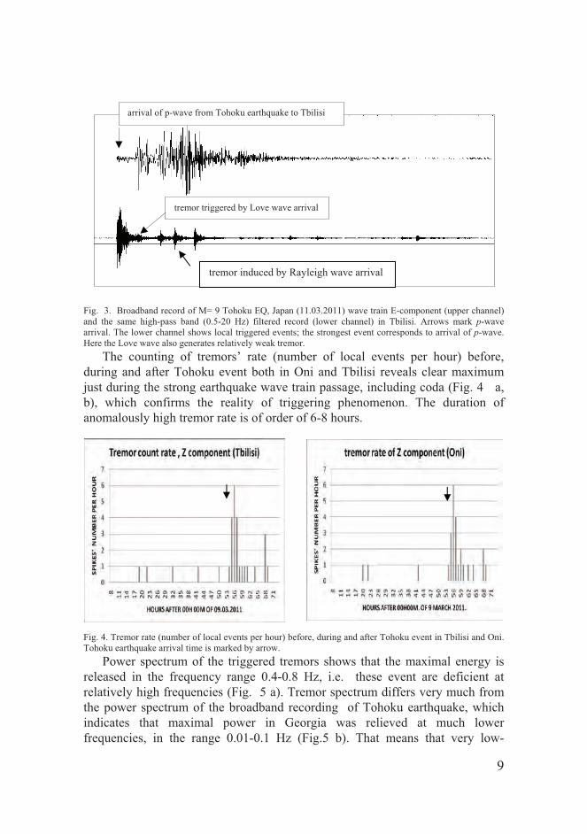
Fig. 3. Broadband record of M= 9 Tohoku EQ, Japan (11.03.2011) wave train E-component (upper channel) and the same high-pass band (0.5-20 Hz) filtered record (lower channel) in Tbilisi. Arrows mark p-wave arrival. The lower channel shows local triggered events; the strongest event corresponds to arrival of p-wave. Here the Love wave also generates relatively weak tremor.

The counting of tremors’ rate (number of local events per hour) before, during and after Tohoku event both in Oni and Tbilisi reveals clear maximum just during the strong earthquake wave train passage, including coda (Fig. 4 a, b), which confirms the reality of triggering phenomenon. The duration of anomalously high tremor rate is of order of 6-8 hours.

Fig. 4. Tremor rate (number of local events per hour) before, during and after Tohoku event in Tbilisi and Oni. Tohoku earthquake arrival time is marked by arrow.

Power spectrum of the triggered tremors shows that the maximal energy is released in the frequency range 0.4-0.8 Hz, i.e. these event are deficient at relatively high frequencies (Fig. 5 a). Tremor spectrum differs very much from the power spectrum of the broadband recording of Tohoku earthquake, which indicates that maximal power in Georgia was relieved at much lower frequencies, in the range 0.01-0.1 Hz (Fig.5 b). That means that very low-

arrival of p-wave from Tohoku earthquake to Tbilisi

tremor triggered by Love wave arrival

tremor induced by Rayleigh wave arrival

10

frequency forcing is necessary for triggering tremors. In other words, forcing of a period 100-10 sec is the time, necessary for tremor area activation.

Fig. 5 a. Spectrum of the largest (first) triggered tremor in Tbilisi. Bandpass Butterworth filter was used to filter data in a range 0.5-20 Hz. b. spectrum of the broadband recording of Tohoku earthquake in Oni.

It seems that not only strong earthquakes, but also middle size remote events also can trigger local earthquakes. For example, it was a surprise to find quite by chance that M=4.6 earthquake in East Greece (09. 03.2003) also triggered local seismicity in Georgia, separated from the epicenter by 1700 km, here again the strongest triggered event coincides with p-wave arrival (Fig. 6 a, b).

a. Oni b. Tbilisi

Fig. 6 a, b. Broadband record of M=4.6 earthquake in East Greece (09. 03.2011) wave train z-component (upper channel) and the same high-pass band (0.5-20 Hz) filtered record (lower channel). The lower channel shows local triggered events; the strongest event corresponds to arrival of p-wave. a. Oni and b. Tbilisi seismic station

This observation needs to be confirmed by good statistics as the result is unexpected. Thus one of the fundamental problems in the project should be

arrival of p-wave from Greece M=4.6 to

triggered

arrival of p-wave from Greece M=4.6 to Oni

triggered events

0.2 0.4 0.6 0.8 1 1.2 1.4 1.6 1.80

0.5

1

1.5

2

2.5

3

3.5

4

Frequency (Hz)

Pow

er S

pect

rum

11

elucidation of magnitudes and distances of remote (forcing) earthquakes and local tectonic environments of sites, where DT phenomenon can be observed.

Rubinstein et al. (2009) and Hill (2010) show clearly (Fig. 7a,b ) that the weak forcing by wave train of remote strong earthquake can not only trigger, but also induce phase synchronization of induced events with surface waves.

Fig.7. Examples of tremor triggered on the Cascadia megathrust beneath Vancouver Island, B.C., by surfaces waves from four Mw >7. 5 earthquake with incidence angles (Rubinstein et al. 2009; Hill, 2010). The top panel in each example shows broadband displacement waveforms for the incident surface waves (bottom three traces) and the high-frequency (5 to 15 Hz) traces for the triggered tremor (upper trace). (a) The Mw 7.9 Denali fault earthquake of 2002, tremor depth �15 km; (b) the Mw 7.5 Oaxaca earthquake of 1999, tremor depth �35 km

The strong resemblance between our experimental results on electromagnetic (Fig. 8) or mechanical synchronization of stick-slip (Chelidze et al, 2006, 2007, 2010) and large scale natural events (Fig. 7) show that the phenomenon of synchronization has universal character and it can be successfully modeled in laboratory.

Fig.8. Acoustic emission (upper channel) during slip after application of 1000 V external periodical voltage (lower channel). Note complete phase synchronization between EM forcing and AE .

The physical mechanism of remote triggering is not clear. The mechanism

should be different for triggered events closely correlated to wave train phase (direct triggering) and for delayed response.

12

Hill (2010) assessed (direct) triggering potential of wave trains from the fracture mechanics point of view, using Mohr and Coulomb-Griffits failure criteria. In general, Love waves incident on vertical strike-slip faults have a greater potential than Rayleigh waves, but the potential of Rayleigh waves incident on dip-slip faults dominates over Love wave potential. At the same time, the fault geometry and frictional strength are variable. Such heterogeneity leads to deviations from the above simple rule.

For large delays frictional failure, subcritical crack growth and excitation of crustal fluids are suggested as appropriate models (Hill, Prejean, 2009; Prejean, Hill, 2009; Hill, 2010).

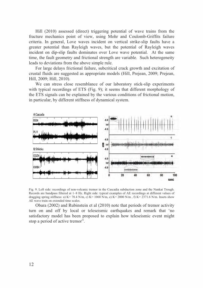
We can stress close resemblance of our laboratory stick-slip experiments with typical recordings of ETS (Fig. 9); it seems that different morphology of the ETS signals can be explained by the various conditions of frictional motion, in particular, by different stiffness of dynamical system.

Fig. 9. Left side: recordings of non-volcanic tremor in the Cascadia subduction zone and the Nankai Trough. Records are bandpass filtered at 1–8 Hz. Right side: typical examples of AE recordings at different values of dragging spring stiffness: a) K= 78.4 N/m, c) K= 1068 N/m, e) K= 2000 N/m , f) K= 2371.6 N/m. Insets show AE wave train on extended time scales.

Obara (2002) and Rubinstein et al (2010) note that periods of tremor activity turn on and off by local or teleseismic earthquakes and remark that ‘no satisfactory model has been proposed to explain how teleseismic event might stop a period of active tremor”.

13

Fig. 10. Distribution of acoustic emission onsets (the left column) and terminations (the right column) relative to the (mechanical) forcing period phase (in twelfths of the forcing period) for different intensities of tangential forcing. Forcing frequency – 80 Hz.

The general explanation of how small-amplitude teleseismic wave can start of stop a period of tremor activity is the extremely high sensitivity of nonlinear systems to a weak forcing. The physical (laboratory) model of mentioned tremor arrest effect has been realized in our experiments with mechanical synchronization of stick-slip (Fig. 10). This remarkable result shows that very small mechanical forcing, 105 times smaller than the main driving force can affect both onsets and terminations of stick-slip generated acoustic wave train.

It seems that further development of sensitive devices, dense networks and processing methods will develop a new avenue in seismology, which can be defined as microseismology and which will study systematically small earthquakes and tremors, especially triggered and synchronized events. These events at present are ignored by routine seismological processing and are not included in traditional catalogues. At the same time, microseismic events contain very important information on geodynamics of processes and can give clues to understanding fine mechanism of nonlinear seismic process and may be, even

14

contribute to the problem of earthquake prediction. Microseismicity can be compared by its importance to studies of elementary particles in physics.

References:

Chelidze, T., O. Lursmanashvili, T. Matcharashvili and M. Devidze. 2006. Triggering and synchronization of stick slip: waiting times and frequency-energy distribution Tectonophysics, 424, 139-155

Chelidze T., and T. Matcharashvili. 2007. Complexity of seismic process, measuring and applications – A review, Tectonophysics, 431, 49-61.

Chelidze, T., Matcharashvili, T., Lursmanashvili, O., Varamashvili N., Zhukova, N., Meparidze. E. 2010. Triggering and Synchronization of Stick-Slip: Experiments on Spring-Slider System. in: Geoplanet: Earth and Planetary Sciences, Volume 1, 2010, DOI: 10.1007/978-3-642-12300-9; Synchronization and Triggering: from Fracture to Earthquake Processes. Eds.V.de Rubeis, Z. Czechowski and R. Teisseyre, pp.123-164

Hill, D. Surface wave potential for triggering tectonic (nonvolcanic) tremor. 2010. Bull. Seismol. Soc. Am. 100, 1859-1878.

Hill, D., Prejean, S. 2009. Dynamic triggering. In: Earthquake seismology, Volume editor H. Kanamori. Elsevier. pp. 257-293.

Matthews, M. and Reasenberg, P. 1988.Statistical methods for investigating quiescence and other temporal seismicity patterns. Pure and Appl. Geophys. 126, 357-372.

Obara, K. 2003. Time sequence of deep low-frequency tremors in the Southwest Japan Subduction Zone. Chigaku Zasshi (J. Geogr.)112, 837-849.

Pikovsky, A., Rosenblum, M.G., Kurths. J. 2003. Synchronization: Universal Concept in Nonlinear Science. Cambridge University Press, Cambridge

Prejean S., Hill, D. 2009. Dynamic triggering of earthquakes. In: Encyclopedia of Complexity and Systems Science, R. A. Meyers (Ed.), Springer, pp. 2600-2621.

Rubinshtein et al. 2010, Non-volcanic tremors. In “New Frontiers in Integrated Solid Earth Sciences. S. Cloetingh, J. Negendank,(Eds), Spronger, Berlin, doi 10.,1007/1007/978-90-481-2737-5. pp. 287-314.

15

VARIATION IN THE SCALING CHARACTERISTICS OF AMBIENT

NOISE AT THE INCREASED LOCAL SEISMIC ACTIVITY

T. MATCHARASHVILI A, B T. CHELIDZE A, Z. JAVAKHISHVILI B, N. JORJIASHVILI B, N. ZHUKOVA A, D. TEPNADZE A a) M. Nodia Institute of Geophysics, Tbilisi, Georgia b) Ilia State University, Tbilisi, Georgia

Abstract. In this research, scaling features of the ambient seismic noise data were investigated in time period of increased local seismic activity around Oni seismic station, Georgia. Data sets of seismic noises recorded at Oni seismic station, located in the area of increased seismic activity, as well as at Tbilisi seismic station, located far from this area, were investigated. In order to quantify scaling properties of ambient noises we used different methods such as power spectrum regression, detrended fluctuation and multifractal detrended fluctuation analysis. It was shown by our analysis, that investigated seismic noise data are long range correlated on large time scales. On smaller time scales by scaling features they look as combination of different stochastic structures typical for multifractal behavior. It was found, that scaling features of seismic noise datasets are noticeably different for seismically active and relatively quiet time periods. Moreover, it was shown that at increased seismic activity Earth surface vibration is closer to persistent long range correlations, while at quiet periods we observe multitude of stochastic behaviors.

Keywords: ambient seismic noise, scaling, multifractal, dynamics.

1. Introduction

It is well known, that earthquakes are as one of the most hazardous

phenomena causing enormous human and economic loses. They occur as a result of complex spatio–temporal processes related to convective motion in the mantle, provoking relative motion of the faults bordering tectonic plates [Kanamori&Brodsky, 2001]. Generated by this motion seismic waves can be

16

detected by seismographs in the form of vibrations of the Earth’s surface. At the same time, seismic waves are not the only cause for the Earth surface vibrations. Many other factors, ranging from atmospheric pressure variation and ocean waves to human activity always contribute to the vibrations of the Earth ground [Yulmetyev, et al. 2001]. These vibrations - microseisms or microtremors, representing superposition of waves of different origin often collectively are named as ambient noises.

Because of their diverse origin and complicated spatio-temporal features earth surface vibrations or ambient noise, represents a random-like high-dimensional dynamical process [Yulmetiev et al. 2001, 2003; Padhy, 2004]. Such highly nonlinear processes normally are characterized by uniform spectral features and dynamical structure, which are extremely difficult to be quantified. On the other hand, seismic signals, contributing to the ambient noise, are regarded as having more regular dynamical structure comparing to random noises [Padhy, 2004; Tabar, et al. 2006; Manshour, et al. 2009]. This is quite logical in the light of established for the last decades presence of nonrandom, though highdimensional dynamical structure in the seismic process – the source of seismic signals [see e.g. Goltz, 1997; Lapenna, 1998; Rundle, 2000; Matcharashvili, 2000; Chelidze&Matcharashvili, 2007]. Presence of nonrandom dynamical structure in the earthquake generation process, and seismic waves accordingly, physically is related to the processes accompanying stress accumulation and the breakdown of a disordered solid together with concomitant stick-slip movement. These complex processes involving cascades of transitions (changes) in wide spatial, temporal and energetic scales generally are, or can be, in principle detectable. Some of these transitions - precursory changes, preceding or accompanying breakdown and stick-slip movement in a disordered solid rocks, have already been observed both at the laboratory and the geophysical scales [Kapiris, 2003; Telesca, 2006; Karamanos, 2006; Chelidze, 2006; Tabar, et al. 2006; Manshour, et al. 2009]. It is also understandable, that because of complexity of seismic process, such changes might be of different forms, related to variations in mechanical, chemical, hydrological, electromagnetic, etc. processes in the seismic source or peculiarities of wave propagation in rocks, e.g. acoustic, electromagnetic emissions [Karamanos, 2006; Tabar et al. 2006].

At the same time, it should be stressed here, that researches about predictive marker changes in earthquake generation still are underway and there are serious debates about precursors, the length of the spatial and time scales over which different precursory anomalous changes may occur and accumulate, etc. At present, there are many pro and contra arguments in this respect. There are contradictions also between supporters of precursory phenomena. Some authors assume, that precursory patterns develop at short spatial distances within few days to weeks before the main shock from impending large earthquakes, while others claim that precursory anomalies may occur up to decades before it at

17

distances much larger than the length of the main shock rupture [Scholz,, 1990; Keilis-Borok, 2002; Tabar, 2006].

Notwithstanding all these difficulties, changes in the dynamical features of ambient surface noise caused by processes related to the earthquake preparation, by many authors are assumed as quantifiable and are regarded among possible precursors [Padhy, 2004; Tabar, 2006; Manshour, 2009, 2010]. Moreover, in the context of possible dynamical changes it was suggested that as the final failure in the disordered media is approached the underlying complexity manifests itself in specific linkages between space and time features. This in turn may lead to the producing of detectable (precursory) patterns on many scales and the emergence of fractal structures in different accompanying process [Karamanos, 2006].

In general the present level of dynamical data analysis enables these changes in dynamical structure of Earth surface vibrations to be assessed qualitatively and quantitatively. Indeed, in last years, a lot of interdisciplinary research works have been devoted to complexity of seismic noises, analysis of their fractal, power law, long memory and many other statistical and dynamical features in order to detect and describe the spatial, temporal and energetic scaling properties of processes related to earthquake preparation [Padhy, 2004; Caserta, 2007; Yulmetyev, et al. 2001; Tabar, 2006].

In the present research we focus on the statistical and fluctuation features of the ambient seismic noise time series using similar concepts. The main goal of this research was to carry out comparative analysis of scaling features of ambient noise time series in the time periods of increased as well as relatively low local seismic activity on the example of seismic data recorded at Oni seismic station in Georgia. Targeted, problem is of general interest and has a great scientific significance, being related to the recognition of changes in apparently similar signals with different physical origins. The recognition of changes caused by arrival of seismic signals in the background random noise is of prime importance from scientific and practical points of views. Such analysis of seismic data often are the subject of vivid interests for different purposes, including earthquake forecasting, and numerous methods of data analysis are used [Caserta, 2007; Yulmetyev, et al. 2001, 2003].

In this work to accomplish targeted research we applied methods often used for time series scaling features analysis for selected seismic noise data sets.

2. Used data and Methods of analysis

Used in this study data are digital seismograms recorded by broad-band

permanent station located in Great Caucasus mountains near town Oni (42.5905N, 43.4525E), Georgia (Fig.1). We investigated all three components of vibrations of Earth’s surface, but mainly focused on time series of fluctuations of

18

the Earth’s vertical velocity, Vz (see typical 4 day recording in Fig. 2). The data were recorded at sampling frequency of 100 Hz with a dynamic range over 140 dB. Station has a flat velocity response from 0.01 to 100 Hz frequency band. The seismograms are corrected for instrument response before analysis so as to get the ground velocity. Seismic station Oni, where analyzed waveforms were recorded, is part of seismic network operated by the Ilia State University, Seismic Monitoring Centre of Georgia.

In order to compare scaling characteristics of ambient noise data sets at different level of local seismic activity, we selected datasets for different time periods. Namely, at first the four-day recordings, prceeding Racha M6.0 earthquake (22:41:35(UTC) on 07.09.2009, Lat. 42.5727, Long. 43.4825) have been investigated.

Fig.1. Map of location of Oni seismic station. By the star epicenter of Racha M6.0 is shown.

In these recordings waveforms arriving from two remote earthquakes are visible. Namely, M4.9 occurred in Afganistan (09:01:53(UTC) on 07.09.2009, Lat. 36.45, Long. 70.73) and M6.2 occurred in Indonesia (16:12:22(UTC) on 07.09.2009, Lat. 10.20, Long. 110.63). Besides, two M1.6 (14:06:35(UTC) on 03.09.2009, Lat. 42.5414, Long. 43.5282) and M2.1 (14:17:31(UTC) on 03.09.2009, Lat. 42.5508, Long. 43.528) foreshocks of Racha earthquake occurred during this 4 day time period. Seismic waveforms from all these events are involved in analyzed time series. So, ambient fluctuations at Oni station in the considered case were affected by strong and weaker local, as well as by remote seismic activities. Next series of analysis were accomplished on seismic record data sets for the time period when no local seismic activity was detected in March 2011. At the end of this time period arrival of waveforms from Japan M9.0 (05:46:24(UTC) on 11.03.2011, Lat. 38.322°N, Long. 142.369°E) earthquake were recorded by Oni station. Additionally, seismic records were

19

considered from 23.59 (UTC) on 21.01.2009 to 19.00 (UTC) on 22.01.2009 when no local and remote seismic activity was detected by broadband Oni station. Other considered time period was from 00.00 (UTC) to 18.59 (UTC) on 30.10.2010, when a slight local seismic activity (series of M1.6, M1.7 events) was detected and waveforms arrived from M5.2 earthquake, occurred in Japan (19:06:19(UTC) on 30.10.2010, Lat. 34.38N, Long. 141.33E).

Fig. 2. The data for the M6.1 Racha earthquake.

In general, complex systems time series, like ambient noise, exhibit fluctuations on a wide range of time scales what often are accompanied by the broad distributions of the values. Such fluctuations usually follow scaling laws, which allow characterization of the data and the generating complex system by fractal (or multifractal) scaling exponents. Knowledge of these scaling exponents is very important because they provide unique information on systems behavior and may serve as characteristic fingerprints for comparison with other systems and models.

In this research in order to quantify scaling features of ambient noise we used three methods for the time series analysis: power spectrum regression, detrended fluctuation analysis (DFA) and multifractal DFA (MF-DFA).

Power spectrum regression exponent calculation enables to elucidate scaling features of ambient noise in the frequency domain. By this method a fractal property of a time series is reflected as a power law dependence between the spectral power (S(f)) and the frequency (f) by spectral exponent β:

)( fS � βf1

20

Spectral exponent β is a measure of the strength of the persistence or anti-persistence, which is related to the type of correlations present in time series [Malamud, 1999; Munoz-Diosdado, 2005]. For example, 0, corresponds to the uncorrelated white noise, whereas short correlated noise or Brownian motion, has a 2, and processes with long-range correlations, such as 1/f noises, exhibit 1.

In order to quantify long-range time-correlations in the investigated ambient noise data sets we used method of DFA [Peng, et al. 1993a,b,1995]. DFA was conceived as a method for detrending local variability in a sequence of events, which provides insight into long-term variation features in the complex data sets. This scaling analysis technique provides a simple quantitative parameter (DFA scaling exponent) representing the correlation properties of a time series. As it was already mentioned the very important practical advantage of DFA over many other scaling techniques is that it enables the detection of long-range correlations embedded in time series. Moreover DFA helps to avoid the spurious detection of apparent long-range correlations that are an artifact of non-stationarity.

In practice DFA method consists of three steps [Peng, 1993a,b]. First initial time series x(k) (of length N), is integrated and “profile” Y(i) is determined . After this the resulting series Y(i) is divided into boxes of size n. In each box of length n, local trend, Yn(i) is calculated. Next, the line points are subtracted from the integrated series Y(i), in each box. The root mean square fluctuation of the integrated and detrended series is calculated:

[ ]2

1)()(1)(

=

−=N

in iYiY

NnF

This process is repeated for different scales (box sizes) to obtain a power law behavior between F(n) and n. When the signal follows scaling law, a power law behavior for the function F(n) is observed:

αnnF ~)(

The scaling exponent gives the information about the long-range power law correlation properties of the signal. Scaling exponent = 0.5 corresponds to white noise (noncorrelated signal), when < 0.5 the correlation in the signal is anti-persistent, if >0.5 the correlation in the signal is persistent. = 1 means uniform power law behavior of 1/f noise and = 1.5 represents a Brownian motion [Peng, 1993,1995]. The value >1.5 corresponds to long-range correlations that may be related to both stochastic and deterministic correlations [Peng, 1995; Rodriguez, et al. 2007]. It may often happen, that the correlations of recorded data do not follow the same scaling law for all considered n time scales. In such cases the function F(n) displays different power-law behaviors and in double logarithmic plots of the DFA fluctuation function, one or more

21

crossovers between different scaling regimes are observed. These crossover (time) scales separate regimes with different scaling exponents [Peng, 1995; Kantelhardt, 2002]. In practice, the crossover region is defined by the values of n where the function F(n) changes its behavior. The relationship between spectral exponent and is given by the formula = (1 + )/2 [Peng, 1993; Iyengar, et al. 1996; Penzel, 2003].

Quantification of the fractal properties through calculation of scaling exponent by above methods is often used to describe features of complex systems behavior. At the same time when dynamics is characterized by, not only one, scaling exponent but by a multitude of scaling exponents we deal with a multifractal process and special methods should be used. One of the effective method to study multifractality in nonstationary signals is multifractal MF-DFA algorithm [Kantelhardt , 2002].

MF-DFA procedure presumes introduction of two additional steps to the standard DFA [Kantelhardt, 2002]. Namely, at first we average over all n segments to obtain the q-th order fluctuation function,

[ ]qqN

inq iYiY

NnF

/1

1

)()(1)( −==

where, in general, the index variable q can take any real nonzero value. For q = 2, the standard DFA procedure is retrieved. As far as we are interested in how the generalized q dependent fluctuation functions Fq(n) depend on the time scale n, for different values of q, calculation should be repeated for different time scales.

MDFA approach has been proposed to study multifractality in nonstationary signals when they are long-range power-law correlated

)(~)( qq nnF α ,

where )(qα is the generalized scaling exponent. For monofractal time series, α (q) is independent of q, and only if small and large fluctuations scale differently, there will be a significant dependence for multifractal data sets.

3. Results and discussions

Total length of considered in our research ambient noise time series was in

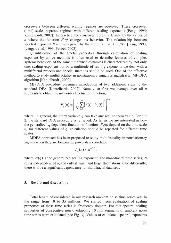
the range from 10 to 35 millions. We started from evaluation of scaling properties of these time series in frequency domain. For this spectral scaling properties of consecutive non overlapping 10 min segments of ambient noise time series were calculated (see Fig. 3). Values of calculated spectral exponents

22

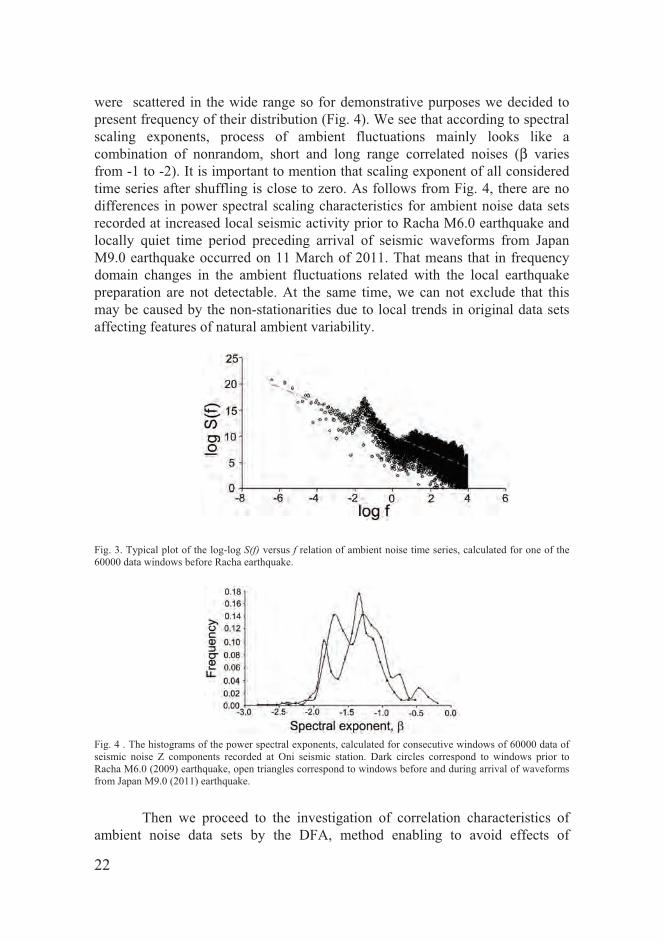
were scattered in the wide range so for demonstrative purposes we decided to present frequency of their distribution (Fig. 4). We see that according to spectral scaling exponents, process of ambient fluctuations mainly looks like a combination of nonrandom, short and long range correlated noises (β varies from -1 to -2). It is important to mention that scaling exponent of all considered time series after shuffling is close to zero. As follows from Fig. 4, there are no differences in power spectral scaling characteristics for ambient noise data sets recorded at increased local seismic activity prior to Racha M6.0 earthquake and locally quiet time period preceding arrival of seismic waveforms from Japan M9.0 earthquake occurred on 11 March of 2011. That means that in frequency domain changes in the ambient fluctuations related with the local earthquake preparation are not detectable. At the same time, we can not exclude that this may be caused by the non-stationarities due to local trends in original data sets affecting features of natural ambient variability.

Fig. 3. Typical plot of the log-log S(f) versus f relation of ambient noise time series, calculated for one of the 60000 data windows before Racha earthquake.

Fig. 4 . The histograms of the power spectral exponents, calculated for consecutive windows of 60000 data of seismic noise Z components recorded at Oni seismic station. Dark circles correspond to windows prior to Racha M6.0 (2009) earthquake, open triangles correspond to windows before and during arrival of waveforms from Japan M9.0 (2011) earthquake.

Then we proceed to the investigation of correlation characteristics of

ambient noise data sets by the DFA, method enabling to avoid effects of

23

nonstationarities in data sets. DFA often is successfully used for data sets of different origin in different fields, including geophysics and seismology [e.g.Telesca, 2005, 2008; Bunde, 2002]. Calculation have been carried out for consecutive 60000 data length non-overlapping windows of ambient seismic noise Z component records for time period of increased local seismic activity, involving seismic waveforms of Racha M6.0 earthquake and its aftershocks and for time period of relatively decreased local seismic activity in March of 2011. By the F(n) vs. n relation for considered two time series three main groups werte distinguished: i. corresponding to windows, when Racha earthquake and its aftershocks occurred, ii. corresponding to the windows, when seismic wavetrains from remote earthquakes (M4.9 occurred in Afganistan, and M6.2 in Indonesia) arrived and iii. Windows, when no local or remote seismic activity was detected by the broadband device of Oni station. Among others, these groups were distinctive by crossover points separating regimes of ambient noise vibrations with different scaling characteristics. It is interesting, that crossovers in F(n) vs. n relation is clearly visible for the third mentioned group (i.e. for the windows when no seismic activity was detected) and not so clearly for the windows, when the remote seismic signals arrive.

In order to visualize general shapes of F(n) vs. n relation for each mentioned three groups, curves of averaged fluctuation values are presented in Figs. 5 to 8. In the upper curve of Fig. 5, we see, fluctuation function F(n) for the time window when strong local Racha earthquake occurred. In the middle curve is presented fluctuation function averaged for all windows for the period, when Racha earthquake aftershock activity was detected. It is known, that for small scales of n, deviations from the scaling law are intrinsic to the usual DFA method [Peng, et al.1993a]. Taking this into consideration, we can regard F(n) vs. n relationships in Fig. 5, as close to linear, despite small crossovers which, it seems can be neglected especially comparing to clear crossovers in curves of other mentioned groups. At the same time the character of Earth surface movement’s fluctuations, related to the strong local earthquake and to its aftershocks seems to be very different. Indeed scaling exponent value for time window when M6.1 Racha earthquake occurred (α=0.82) indicates persistent, long-range power law correlation in the ambient noise [Peng, et al. 1995]. Contrary to this during aftershock period fluctuations reveal clear anti-persistent power law behavior (α=0.30). In this antipersistent case, as it is known, increment of fluctuations should very likely followed by decrement what obviously shows that system gradually is approaching condition close to equilibrium, when local seismic activity decreases. These differences between correlation features of considered time windows obviously express real situation and can not be regarded as artifact of calculation. Indeed, randomized ambient noise time series do not preserve any internal dynamical structures and shuffled time series (see Fig. 5, lower curve) looks like white uncorrelated noise (α=0.50).

24

Fig. 5. DFA fluctuation curves obtained for Z constituent of seismic noise records at Oni seismic station. Upper curve was calculated for 60000 data window which contained waveforms of Racha Eq (DFA scaling exponent α1), middle curve corresponds to averaged fluctuation function for time windows when aftershocks of Racha earthquake occurred (DFA scaling exponent α2). Lower curve corresponds to the fluctuation function (DFA scaling exponent α3) of the shuffled ambient noise, averaged for all 570 windows of data set. Curves are shifted along the y axis for clarity. In Fig. 6, results of ambient noise DFA analysis are presented, for time windows when no local earthquakes occurred. Exactly we focused on time windows when at Oni station: a) only arrivals of waveforms from remote earthquakes were detected and b) neither local earthquakes occurred nor arrival of wavetrains from remote earthquakes were registered. In the upper curve of Fig. 6, averaged DFA fluctuation curve of ambient seismic noise data is presented for windows when wavetrains arrival of remote earthquakes have been detected, exactly we mean events occurred in Afganistan M4.9 and Indonesia M6.2 (see methods section for details). We see crossover on this curve about 10-15 sec time scale. At the same time averaged DFA fluctuation curve calculated for ambient noise data recorded at the quiet time windows, clearly shows presence of two crossovers. Exactly, calculations in this last case, have been made in the time period prior to Racha M6.0, for selected 500 windows of 60000 data each, when no local earthquakes as well as arrival of waveforms from remote events been detected (lower curve in Fig. 6). Time scales of these crossovers are about 0.5 and 10 sec and they might be related to high frequency components of ambient noises.

Thus, Fig. 6, shows, presence of crossover at about 10 sec time scale in ambient noise fluctuations, both in the quiet time windows and for time windows when waveforms from remote earthquakes arrived. Above this crossover, scaling exponent drastically decreases indicating strong antipersistence almost close to the lack of power law scaling behavior (calculated scaling exponent values are 0.07 and 0.1 accordingly). At smaller time scales we observe different behavior of ambient noise fluctuations in quiet windows and in time windows when remote seismic waveforms arrived. In the last case, there are no further crossovers and scaling exponent (α >1.5) indicates long range correlations which may be related to stochastic process. Contrary to this in quiet windows (lower curve in Fig. 6), crossover occurs at about 0.5 sec time scale below which long range correlation behavior, detected at larger scales (scaling exponent equal

25

to 1.60), is replaced by the Brownian motion like process with close to 1/f behavior (scaling exponent 1.14).

Fig.6. Crossovers of averaged DFA fluctuation curves obtained for Z constituent of seismic noise records at Oni seismic station. Lower curve corresponds to windows of quiet periods when no local earthquakes as well as arrival waveforms from remote earthquakes have been registered before M6.1 Racha earthquake (2009) (α1 slopes), upper curve corresponds to windows when arrival of waveforms from remote earthquakes were registered (α2 slopes).

Comparing data sets with activated and quiet seismic patterns, in order to be focused on the changes possibly related to the local earthquake preparation, we decided to exclude influence of all signals regarded as seismic waveforms both from locally occurred as well as remote events. For this we selected time windows from both considered ambient noises data series, when no local or remote activity was detected at Oni seismic station and calculated DFA fluctuation functions for them. Results are shown in Fig. 7. From these results we see crossover at the mentioned above 10 sec time scale. Above this time scale, fluctuation are antipersistent both in the time period prior to Racha earthquake (α1 =0.07+/-0.01) and for quiet time period, prior to arrival of Japan earthquake waveforms, (α2 =0.14+/-0.01). Looking at the smaller scales, we see additional crossover at about 0.5 sec time scale for time period prior to Racha earthquake, while in case of time period prior to Japan earthquake crossover still seems to be visible, but it is questionable whether for small scale such small difference between slopes might be indeed detectable (see Fig. 7, left lower part of dark curve). Between these 10 and 0.5 sec crossovers fluctuations of ambient noise always reveal long range correlations (α>1.5). Below 0.5 sec scale for time period before arrival of wavetrains from Japan earthquake, there are no changes in fluctuations. Contrary to this, for time period prior to Racha earthquake fluctuation become close to 1/f noise- like (in Fig. 7, α1 =1.14+/-0.01). Results in Fig. 7, show that different dynamical structures with respect to

26

scaling behavior are present in a considered ambient noise data for seismically quiet and active time periods around Oni station.

Fig. 7. Crossovers of averaged DFA fluctuation curves obtained for Z component of seismic noise records at Oni seismic station. Open triangles correspond to time windows of quiet periods preceding M6.0 Racha earthquake (2009) (α1 slopes), dark triangles corresponds to windows prior to arrival of wavetrains from remote Japan M9.0 earthquake 2011 ( α2 slopes).

Thus considered DFA fluctuation curves show different power laws for different time scales, revealing interesting inherent properties of Earth surface vibrations for different patterns of local seismic activity. At the same time, to have kind of coarse-graining estimation of some general features of ambient noise fluctuations, for each sliding windows we also calculated integral scaling exponents. This helped to simplify the DFA-based analysis of complicated data and to grasp the basic scaling tendencies in ambient seismic noises. Integral slopes of averaged, fluctuation curves were also calculated. For example, integral scaling exponents calculated for time windows prior to M6.0 Racha earthquake, in which remote events have been or have not been registered, equal to αint(re) =1.26+/-0.03, and αint(wre) = 0.92+/-0.02 accordingly. On the other hand integral scaling exponent calculated for averaged F(n) vs. n relation in seismically quiet period prior to arrival of seismic signals from Japan M9.0 earthquake equals αint(r) =1.13+/-0.04 (Fig. 7, upper curve).

According to these results on full range of analyzed time scales, in seismically quiet time periods ambient noise fluctuations are close to 1/f type process and somehow become closer to Brownian motion when wavetrains from remote events arrive. On the other hand for time periods of increased local seismic activity scaling exponent of ambient noise time series decreases, revealing persistent long range correlation.

In order to better compare scaling properties of complicated ambient noise data sets for different time periods we performed additional statistical and distributional analysis of obtained DFA results. In Fig. 8, histograms of the

27

scaling exponents calculated for consecutive windows of 60000 data are presented for about 90 hour time period containing Racha M6.1 earthquake with aftershocks and 80 hour time period involving arrival of seismic wavetrains from Japan M9.0 earthquake.

In the left side of Fig. 8, histograms of scaling exponents calculated for the same time series after shuffling procedure are presented. We see that more than 95% of scaling exponent values for shuffled data sets are concentrated close to 0.5 value corresponding to white noise (the significance of difference between the scaling exponents for original and shuffled data sets was quantified by the method described in Theiler at al. [1992]). Contrary to this, original time series, by their DFA scaling exponents, are always strongly different from random walk or antipersistent behavior (curves in the right side of Fig. 8 and 9). At the same time histograms in the right side of Fig. 8, indicate important differences in the Earth surface fluctuation properties for the two considered time periods. We see that not less than 90% of values of calculated DFA scaling exponents, for time period of strong local Racha earthquake, correspond to persistent long range correlated process (dark circles). On the other hand we observe essential shift to the larger DFA exponents for seismic noise data, recorded at locally quiet period when seismic waves from remote Japan M9.0 earthquakes have been detected. In this case more than 97% of calculated DFA scaling exponents exceed value 1, spanning over wide range to about 1.8. These different kinds of fluctuation characteristics, with respect to scaling behavior, demonstrates different stochastic structures in ambient noises data sets for different patterns of local seismic activity. Moreover, we see two maxima in the curve, about 1.1 and 1.5 (white circles in Fig. 8 and 9). This result indicates, that at the quiet period ambient seismic noise comprise multitude of diverse processes from uniform power law behavior of 1/f type ( = 1) to long-range correlations which may be of stochastic fractional Brownian motion or even of deterministic nature ( >1.5), involving also Brownian motion type processes ( =1.5).

Statistically significant difference in mean values of integral scaling exponents for these two groups ( avgR =0.92+/-0.10, , avgJ =1.28+/-0.19, P<0.001) also provides additional argument in favor that the dynamics of seismic noises in considered time periods is different. It is of special importance to underscore, that this difference is not caused by the influence of seismic component of ambient noise (i.e. by waves from local or remote earthquakes). Indeed, the result was practically the same when we selected only quiet time windows (when arrival of seismic waves from local or remote earthquakes have not been detected at Oni station).

28

Fig.8. The histograms of the integral scaling exponents calculated for consecutive windows of 60000 seismic noise Z components data sets recorded at Oni seismic station. Dark circles correspond to 500 windows involving time periods prior to Racha M6.1 EQ, dark triangles correspond to 400 windows in March of 2011 involving time period before arrival of seismic waves from Japan M7.9 EQ. Open circles and triangles correspond to shuffled data sets.

0

0.05

0.1

0.15

0.2

0.25

0.3

0.35

0.5 0.6 0.7 0.8 0.9 1 1.1 1.2 1.3 1.4 1.5 1.6 1.7

DFA scaling exponents

Freq

uenc

y

Fig.9. The histograms of the integral scaling exponents calculated for consecutive windows of 60000 seismic noise Z components data sets recorded at Tbilisi seismic station. Dark circles correspond to windows involving time periods prior to Racha M6.1 EQ, open circles correspond to windows in March of 2011 involving time period before arrival of seismic waves from Japan M7.9 EQ.

The origin of the shift to the more correlated behavior at increased local

seismic activity remains mostly unclear, though it may be speculated that it is related to the decrease of complexity in the Earth surface vibration dynamics under influence of earthquake preparation processes. Findings that ambient noise have higher fractal dimension than the seismic signals, and that probability density function (PDF) of ambient noise may undergo the transition from a Gaussian to a long tailed non-Gaussian prior to moderate and large earthquakes, are in agreement with our results [Padhy, 2004; Tabar, et al. 2006;Manshour, et al. 2009, 2010].

It can be suggested that the shift to the more correlated behavior prior to increased seismic activity can be also detected in other non seismic processes,

29

related to earthquake generation. Indeed, recent analysis of the temporal evolution of the fractal characteristics of preseismic electromagnetic emission indicates, that the earthquake nucleation phase approach is accompanied by a significant reduction of complexity and transition to the persistent behavior [Karamanos, et al. 2006].

Prevalence of DFA scaling exponent values larger than 1 was found also for EW and NS components time series of ambient noise data sets recorded for time period before Japan M9.0 earthquake in March 2011.

As an additional arguments that differences observed between time periods of increased and decreased local seismic activity can not be regarded as artifact of analysis we present results in Fig. 10.

a.

b.

Fig.11. The histograms of the DFA scaling exponents calculated for consecutive windows of seismic noise Z components data sets recorded at Oni seismic station in time period prior and during, a) Racha M6.0 earthquake occurrence, 2009 and b) arrival of seismic waveforms from Japan M9.0 earthquake. Length of sliding windows: 30000 – asterisks, 60000 –triangles, 120000 – circles.

Among others it was necessary to take into consideration, that the length of time series may affect results of the scaling exponent calculation [Peng, 1995; Rodriguez, 2007]. Namely, we needed to be convinced, that spurious conclusions about calculated scaling exponents values, because of the lengths of

30

time series windows, for which actual DFA was accomplished (i.e.10 min duration 60000 data segments), have been avoided. For this, we repeated mentioned above analysis for shorter and longer sliding windows. In Fig. 10, we present histograms of DFA scaling exponent values calculated for large and shorter time windows. As we see, distribution of scaling exponent values indeed is influenced by length of selected time windows. For the time period of activated local seismicity, the longer is the time window, the more demonstrative is persistence of ambient noise fluctuations. Indeed, if for the 30000 data length windows we observed about 50% of values corresponding to the persistence of ambient noise fluctuations, for the longer 60000 and 120000 data windows, the portion of calculated scaling exponents values corresponding to the persistent correlations, increased to about 90% and 97% accordingly (Fig. 10. a). It is important, that shift to the persistence values we observe also for longer time windows at periods of decreased local seismic activity, namely, for ambient noise data recorded in March 2011 prior to arrival of wavetrains from Japan M9.0 earthquake. At the same time, in this case we also see, that the characteristic long right tail, observed for data sets recorded at seismically relatively quiet period, is retained for all selected windows length (Fig. 10, b). Moreover, overwhelming majority of calculated DFA exponent values are in the range mentioned above (1-1.8), independently from time window length selected. Thus, we conclude that general features of differences in distributional features between DFA scaling exponent values calculated for the seismically active and quiet periods are not affected by the length of selected windows and that 10 min duration windows are optimal for our analysis.

Then, in order to exclude inaccuracies because of possible specificities of analyzed time periods, we tested our results for two additional time periods. For this, we aimed to select one to several days length time periods with as low as possible local seismic activity as well as additional time period with moderate local seismic activity. Exactly, from the data sets of ambient noises recorded at Oni seismic station 20 hour period from 00.00 to 19.00 (UTC) on 10.30. 2010 was selected. As it was mentioned in the section on used data and methods seismic activity around Oni station in this period was slightly increased and besides, at the end of the selected time interval arrivals of seismic waves from M6.4 earthquake occurred in Japan were detected. The next time period was selected from 23.59 to 19.00 (UTC) on 01.01.2009. During this period and immediately before and after it, no increase of local seismic activity has been observed and arrival of seismic waves from remote earthquakes also was not detected.

31

Fig.11. The histograms of the DFA scaling exponents calculated for consecutive of 60000 data windows of seismic noise Z components recorded at Oni seismic station. Dark circles - time period in March 2011 before Racha M6.0 event, dark triangles - time period from 00.00 to 19.00 on 10.30.2010, open triangles - from 23.59 to 19.00 on 01.01.2009, open circles - time period before and during Japan M9.0 earthquake, 2011.

For these two additional time periods calculations of DFA scaling

exponents, similar to described above, have been carried out. In Fig. 11, results of these calculations are presented in the form of histograms of integral DFA scaling exponents. It can be seen that for period of slightly increased local seismic activity distribution of scaling exponents resembles the pattern, observed in the period, when the strong M6.0, Racha earthquake occurred. Namely, on the whole considered time scales ambient noise reveals prevalence of persistent long range correlations (black triangles in Fig. 11). In turn, for the period regarded as the calmest among considered ones (with no local or remote events registered at Oni), in the beginning of 2009 we see distribution (open triangles in Fig.11), which reveals important similarity with the pattern in the locally quiet time period in March of 2011, before arrival of waves from Japan M9.0 earthquake. In this case values of DFA scaling exponents are distributed in a wide range, indicating coincidence of different dynamical behaviors without dominate type of correlation in ambient noises.

Such behavior of ambient noise fluctuations at locally quiet time windows, when a multitude of scaling exponents are involved is typical for phenomenon of multifractality. At the increased local seismic activity, prior to Racha M6.0 event in 2009, ambient noises also can not be regarded as monofractal. In this last case the range of the scaling exponent values, is not as wide as for quiet period, but still is wide enough and excludes the possibility to describe the process by a single scaling exponent. Thus for the further analysis of scaling features of ambient noise time series multifractal analysis technique was applied.

As it was described in method’s section, we used MF-DFA analysis technique [Kantelhardt, et al. 2002] to assess multifractal features of ambient noise time series. This approach is based on the identification of scaling of qth-order moment depending on signal segment length, and it is generalization of

32

standard DFA method in which q = 2. In the light of mentioned above wide range of scaling exponents necessary to describe ambient noise fluctuations, it is quiet logical that in Fig. 12, where the results of MF-DFA are presented, we see typical for multifractal sets, H(q) vs. q dependence for data sets from both seismically active and relatively quiet periods. At the same time, multifractal pattern is more pronounced in the case of locally quiet time period before arrival of seismic waves from Japan earthquake in March of 2011 (dark triangles in Fig. 12).

From the theory of multifractal analysis it is known, that for positive values of q, h(q) describes scaling behavior of time segments with large fluctuations (i.e. large variance of F(n) - at large deviation from the corresponding fit). In its turn for negative values of q, h(q) describes scaling behavior of time segments with small fluctuations. Bearing this in mind we can conclude from Fig. 13, that at increased local seismic activity (dark circles) small fluctuations in ambient noise dominate, while at decreased local seismic activity (dark triangles) prevail large fluctuations.

Fig. 12. The generalized Hurst exponent H(q) versus q calculated for the seismic noise Z component time series. Filed circles and triangles correspond to the period before M6.0 Racha earthquake (2009) and period preceding arrival of waveforms of Japan M9.0 earthquake (2011) accordingly. Open circles correspond to shuffled data sets.

One of the subjects of special interest in scaling behavior analysis is the determination of the source of multifractality. The easiest way for this is to analyse corresponding shuffled and surrogate time series. In general, two different types of multifractality in time series can be distinguished: 1) multifractality due to a fatness of PDF of the time series and 2) multifractality due to different correlations in small and large scale fluctuations. When multifractality is related with fatness of PDF, it cannot be removed by shuffling procedure, while in the second case corresponding shuffled time series will exhibit monofractal scaling, since all long-range correlations are destroyed by shuffling procedure. It may also happen, that both types of multifractality are

33

present. In such cases shuffled series will show weaker multifractality than original series [Kantelhardt, et al. 2002].

As follows from the results presented in Fig. 12, shuffling procedure destroys correlation structure of ambient noise data sets in both considered cases, at increased (open circles) and decreased (open triangles) local seismic activity around Oni seismic station. H(q) values calculated for shuffled series are concentrated in the vicinity to 0.5 exhibiting nonmultifractal scaling [Kantelhardt, at al. 2002]). At the same time, observed scaling can not be regarded as clearly monofractal, rather there is weaker type of multifractality in shuffled ambient noise data. This can be interpreted as the situation, when observed multifractality mainly is related to correlations and in lesser degree to the distributional features of analyzed data sets.

Thus, though, at increased seismic activity the dynamics of ambient noise fluctuations looks somehow closer to monofractality, there are more arguments to conclude, that in both considered cases we deal with process characterized by multifractal scaling. At the same time in spite of this qualitative similarity ambient noises for time periods of increased and decreased local seismic activities reveal quantitative differences in their long-range correlation properties.

4. Conclusions

On the example of seismic noise data sets recorded at Oni seismic station, we have shown that, in general for wide time scale, ambient noise data sets are characterized by long range correlations. At the same time, on several smaller time scales ambient noise may contain a mixture of different stochastic structures demonstrating different scaling behavior, including both types of persistence, random walk, Brownian behavior, etc.

Fluctuation properties of ambient noise are essentially affected by influence of seismic waves from both local and remote earthquakes. Scaling properties of ambient noise prior to earthquake occurrence during increased local seismic activity may be quantifiable. Increased seismic activity is accompanied by the persistent scaling behavior on large scales, while for seismically quiet periods the Browniain-type processes prevail.

In periods of both increased or decreased seismic activity, ambient noise reveals multifractal properties. At the same time character of multifractality is different for different levels of local seismic activity. By comparing the second moment exponent of original time series with the shuffled one’s, we have found that the largest contribution to multifractality is due to correlations in noise data sets.

34

References

Bunde, A., J. Kropp, and H. J. Schellnhuber (2002), The Science of Disasters: Climate Disruptions,

Heart Attacks, and Market Crashes, Springer-Verlag, Berlin. Caserta, A., G. Consolini, P. De Michelis (2007), Statistical Features of the seismic noise-field, Stud.

Geophys. Geod. 51, 255-266. Chelidze, T., Lursmanashvili O., Matcharashvili T., Devidze, M., (2006), Triggering and

synchronization of stick slip: Waiting times and frequency-energy distribution, Tectonophysics, 424, 3-4, 139-155

Chelidze, T., Matcharashvili, T., (2007), Complexity of seismic process; measuring and applications—A review. Tectonophysics 431, 49–60.

Goltz, C., (1997), Fractal and Chaotic Properties of Earthquakes, Lecture Notes in Earth Sciences, 77, Springer, Berlin.

Iyengar, N., C.-K. Peng, R. Morin, A. L. Goldberger, and L. A. Lipsitz (1996), Age-related alterations in the fractal scaling of cardiac interbeat interval dynamics, Am. J. Physiol. 271, R1078–R1084.

Kanamori, H., and E.E. Brodsky (2001), The physics of earthquakes, Physics Today. 54, 34–40. Kantelhardt, J. W., S. A. Zschiegner, A. Bunde, S. Havlin, E. Koscielny-Bunde, and H. E. Stanley

(2002), Multifractal detrended fluctuation analysis of nonstationary time series, Physica A. 316, 87-114 .

Kapiris, P. G., K. A. Eftaxias, K. D. Nomikos, J. Polygiannakis, E. Dologlou, G. T. Balasis, N. G. Bogris, A. S. Peratzakis, and V. E. Hadjicontis (2003), Evolving towards a critical point: A possible electromagnetic way in which the critical regime is reached as the rupture approaches, Nonlinear Processes in Geoph. 10, 511–524.

Karamanos, K., D. Dakopoulos, K. Aloupis, A. Peratzakis, L. Athanasopoulou, S. Nikolopoulos, P. Kapiris, and K. Eftaxias (2006), Preseismic electromagnetic signals in terms of complexity, Phys. Rev. E. 74, 016104.

Keilis-Borok, V. I., and A. A. Soloviev (2002), Nonlinear Dynamics of the Lithosphere and Earthquake Prediction, Springer, Heidelberg.

Lapenna, V., M. Macchiato, and L. Telesca (1998), 1/f Fluctuations and self-similarity in earthquake dynamics: observational evidences in southern Italy, Physics of The Earth and Planetary Interiors. 106, 1-2, 115-127.

Malamud, B. D., and D. L. Turcotte (1999), Self-affine time series I: Generation and analyses, Adv. Geophysics. 40, 1-90.

Manshour, P., S. Saberi, Muhammad Sahimi, J. Peinke, Amalio F. Pacheco, and M. Reza Rahimi Tabar (2009),Turbulent-Like Behavior of Seismic Time Series, Phys. Rev. Lett. 102, 014101.

Manshour, P., F. Ghasemi, T. Matsumoto, J. Gómez, M. Sahimi, J. Peinke, A. F. Pacheco, and M. R. R. Tabar (2010), Anomalous fluctuations of vertical velocity of Earth and their possible implications for earthquakes, Phys. Rev. E. 82, 036105.

Matcharashvili, T., Chelidze, T., Javakhishvili, Z., (2000), Nonlinear analysis of magnitude and interevent time interval sequences for earthquakes of Caucasian region, Nonlinear Processes in Geophysics, 2000, 7, 9-19.

Munoz-Diosdado, A., L. Guzman-Vargas, A. Rairez-Rojas, J. L. Del Rio-Correa, F. Angulo-Brown (2005), Some cases of crossover behavior in heart interbeat and electoseismic time series, Fractals. 13, 4, 253-263.

Padhy, S. (2004), Rescaled range fractal analysis of a seismogram for identification of signals from an earthquake, Current Science. 87, 5, 637-641.

Peng, C.-K., S. V. Buldyrev, A. L. Goldberger, S. Havlin, M. Simons, and H. E. Stanley (1993), Finite size effects on long-range correlations: implications for analyzing DNA sequences, Phys. Rev. E. 47, 3730-3733.a.

Peng, C. K., J. Mietus, J. Hausdorff, S. Havlin, H. E. Stanley, and A. L. Goldberger (1993), Long-Range Anticorrelations and Non-Gaussian Behavior of the Heartbeat, Phys. Rev. Lett. 70, 1343-1346.b.

35

Peng, C. K., S. Havlin, H. E. Stanley, and A. L. Goldberger (1995), Quantification of scaling exponents and crossover phenomena in nonstationary heartbeat time series, Chaos. 5, 82–87.

Penzel, T., J.W., Kantelhardt, L., Grote, J. H., Peter, and A. Bunde (2003), Comparison of detrended fluctuation analysis and spectral analysis for heart rate variability in sleep and sleep apnea, IEEE Transactions on Biomedical Engineering. 50, 10, 1143-1151.

Rodriguez, E., J. C. Echeverria, and J. Alvarez-Ramirez (2007), Detrended fluctuation analysis of heart intrabeat dynamics, Physica A: Statistical Mechanics and its Applications. 384, 2, 429-438.

Rundle, J. B., D. L. Turcotte, and W. Klein (2000), GeoComplexity and the Physics of Earthquakes. In: J. B. Rundle, D. L. Turcotte and W. Klein (eds), AGU Monograph 120, American Geophysical Union, Washington, DC, 1-3.

Scholz, C. H. (1990), The Mechanics of Eathquakes and Faulting, Cambridge University Press, Cambridge.

Telesca, L., V. Lapenna, M. Macchiato (2005), Multifractal fluctuations in seismic interspike series, Physica A. 354, 629–640.

Telesca, L., and V. Lapenna (2006), Measuring multifractality in seismic sequences, Tectonophysics. 423, 1-4, 115-123.

Telesca, L., M. Lovallo, V. Lapenna, M. Macchiato (2008), Space-magnitude dependent scaling behaviour in seismic interevent series revealed by detrended fluctuation analysis, Physica A. 387, 3655–3659.

Theiler, J., S, Eubank, A. Longtin, B. Galdrikian, and J. D. Farmer (1992), Testing for nonlinearity in time series: the method of surrogate data, Physica D. 58, 77–94.

Tabar, M. R. R., M. Sahimi, F. Ghasemi, K. Kaviani, M. Allamehzadeh, J. Peinke, M. Mokhtari, M. Vesaghi, M. D. Niry and A. Bahraminasab, et. al. (2006), Short-Term Prediction of Medium and Large-Size Earthquakes Based on Markov and Extended Self-Similarity Analysis of Seismic Data, Modelling Critical and Catastrophic Phenomena in Geoscience, Lecture Notes in Physics. 705, 281-301, DOI: 10.1007/3-540-35375-5_11.

Yulmetyev, R., Gafarov, F., Hanggi, P., Nigmatullin,R., Kayumov, S,(2001), Possibility between earthquake and explosion seismogram differentiation by discrete stochastic non-Markov processes and local Hurst exponent analysis, Phys. Rev. E, 64, 066132

Yulmetyev, R., Hanggi, P., Gafarov, F., and D.G. Yulmetyeva (2003), Non-Stationary Time Correlation in Discrete Complex Systems: Applications in Cardiology and Seismology, Nonlinear Phenomena in Complex Systems. 6:3, 791 – 799.

36

PROCESSING RUSSIAN AND EUROPEAN EARTH OBSERVATIONS

FOR EARTHQUAKE PRECURSORS STUDIES (PRE-EARTHQUAKES)

AND TUBITAK MRC’S ROLE IN THE PROJECT

ERHAN ALPARSLAN, SEDAT NAN, ÖMER V. SARIKAYA TUBITAK Marmara Research Center (MRC) Earth and Marine Sciences Institute Gebze-Kocaeli-Turkey

erhan.alparslan@mam.gov.tr

Abstract. This paper aims to introduce the PRE-EARTHQUAKES project funded by the EC 7th Frame Program and discusses the role played by the Earth and Marine Sciences Institute of TUBITAK’ s Marmara Research Center. The project took a start by the kickoff meeting held at Potenza, Italy, between 15-16 March, 2011, by the project coordinator, University of Basilicata, Department of Engineering and Physics of the Environment and will finish by the end of year 2012. The objectives of the project, the motivation behind, the methodologies that will be employed, the observational capabilities of all the project partners and their roles in the project are also briefly mentioned.

Keywords: Earthquake precursors, EU and Russian Earth Observation

1. INTRODUCTION

Implementation of an operational earthquake prediction system has been impossible so far due to inexistence of a reliable and effective parameter to be measured or an observational methodology to be used. However, combined use of different observations/parameters together with the refinement of data analysis methods may give major improvements on reliability and precision of predictions reducing false alarms. European Union and Russia play a worldwide scientific leading role in this research field. Therefore, successful results may be obtained in earthquakes precursors studies by integrating their data and methodologies (PRE-EARTHQUAKES Project Proposal Part B, 2009).

37

2. OBJECTIVES

The objectives of PRE-EARTHQUAKES may be simply defined as committing researchers from European Union and Russia to integrate different observational data (including ESA and ROSKOSMOS satellite data) and to improve by cross-validating their methodologies in order:

• To improve substantially knowledge of preparatory phases of earthquakes and their possible precursors

• To provide a worldwide EQuOS (Earthquake Observation System) as part of GEOSS (Global Earth Observation System of Systems)

• To develop and offer to the international scientific community a common integration platform (PEG) where

• independent observations and • new data analysis methodologies devoted to research on/of

earthquake precursors can be collected and cross validated.

The scientific objectives of PRE-EARTHQUAKES may be listed as: • coordination and realization of a systematic data acquisition and product

generation system in predefined standardized output formats. • definition and implementation of a common platform where

heterogeneous data inputs can be handled, organized and compared. • validation and dissemination of data analysis and integration

methods/tools making them available and open to the contribution of the worldwide scientific community in order to further extend the number of contemporary monitored parameters and to improve the quality of data analysis methods.

3. MOTIVATION

The motivation behind PRE-EARTHQUAKES was – to demonstrate and consolidate the high potential of EU+Russia research

system in the frontier research field of earthquake precursors To profit from the unique occasion of having free access to valuable ESA and ROSKOSMOS satellite data

– To consolidate scientific collaboration among Russian and European researchers in a very challenging and poorly funded research area

– To have the opportunity to contribute to a significant improvement of the knowledge of preparatory phases of earthquakes and their possible precursors

38

4. METHODOLOGY

The project started with a kick-off meeting in Italy at the coordinator premises which was mainly devoted to sharing of knowledge on the partners’ data analysis methodologies and their capabilities of generating data products. There was a first discussion of I/O interfaces and functions to be activated on a common integration platform (PEG). Then possible problems (e.g. data availability) for each already identified test case were identified. The project is planned to proceed following few other simple actions:

• Starting data acquisition and product generation for selected test case (earthquakes in Italy, Turkey, Sakhalin region) in the past

• Setting-up of the PEG platform (including web site) • Evaluation of system performances by integrating/comparing different

data/methods always using a validation/confutation approach in order to identify anomalous transients actually related to earthquakes occurrence

• Starting real-time monitoring on the base of the best choice of parameters/methods done at previous point.

5. DATA TO BE INTEGRATED

Taking the earth observation capabilities of the project’s partners into account, the following data was considered for integration:

• Ionosphere o TEC (total electron content)

• Near surface low atmosphere o Solar reflected earth’s thermally emitted radiation o MW thermally emitted radiation o Earth’s thermally emitted radiation o VS-NIR spectral signatures in reflectance

• Lithosphere o Concentration of ground radon o Magnetic and electric fields, electrical resistivity

39

Figure 1. Elaz� test case

6. TEST CASES

3 test cases at three different locations were selected for validation and confutation of the results obtained by the methodology employed in this project. These events are:

• Abruzzo earthquake of April 6, 2009 in Italy • Elaz� earthquake of March 8, 2010 in Turkey (See Fig.1) and • Nevelsk earthquake of August 2nd, 2007 in Russia

7. TUBITAK’MRC’S ROLE IN THE PROJECT

PRE-EARTHQUAKES project partner, Earth and Marine Sciences Institute is one of the six Institutes of Marmara Research Center of TUBITAK, which is a research and technology center conducting strategic researches in the areas of Natural Resources and Natural Hazards of Geological Origin using advanced technology based on measurements, monitoring and computer-aided modeling. Ground observation capabilities of Earth and Marine Sciences Institute (See Figure 2) expanded mainly within the framework of multi-disciplinary earthquake research project in the geostrategic regions of Turkey (2005-2010) to include 55 radon gas, 42 spring water, 72 micro-seismological and 136 GPS monitoring stations along the Northern Anatolian Fault, Eastern Anatolian Fault and Aegean Extensional System, which are responsible from 60% of the

40

earthquakes occurring in the country. The important findings based on evaluation of modeling of the continuous data acquired were published by the group (some examples are: nan et al., 2010; nan and Seyis, 2010, Seyis et al., 2010, Baykut et al., 2010; Ergintav et al., 2009, Tan et al., 2010)

Figure 2. Observation capability of TUBITAK MRC

TUBITAK MRC’s role in the project is to provide daily continuous land observations (soil radon, spring water) ( nan and Alparslan, 2011). It expects to receive daily TIR anomaly maps prepared by other project partners and daily process of GPS time series identification of possible ionospheric anomalies and a user friendly and practical GPS processing software to be sharedç

8. PARTNERS AND THEIR ROLES

The project coordinator is Department of Engineering and Physics of Environment of University of Basilicata, which works in a 20 year scientific collaboration with CNR(Italian National Research Council)/IMAA(Institute of Methodologies for Meteorological Analysis). They will provide TIR anomalies maps by RETIRA index and RST technique using earth’s thermally emitted radiation acquired by ESA’s MSG/SEVIRI, EOS/MODIS and NOAA/AVHRR and electrical resistivity profiles using time series data analysis.

DLR (German Aerospace Center) has expertise in ionosphere sounding, and regional/global total electron content monitoring, which will be used in project.

FIAG (Fiodorov Institute of Applied Geophysics) is responsible for space weather monitoring and prediction using satellite and ground based observations. It has the system of meteorological satellites, METEOR-M and geostationary satellites ELEKTRO where solar terrestrial relations parameters are measured. They will provide GPS/MET and GPS TEC maps to the project.

41

RSS (Russian Space Systems) has been involved in a number of space projects and will contribute electron concentration maps, humidity profiles and anomaly cloud structures to PRE-EARTHQUAKES project.

WD-IZMIRAN (Pushkov Institute of Terrestrial Magnetism, Ionosphere and Radio Wave propagation of the Russian Academy of Sciences Western Department will provide different kind of data products based on GPS measurements in order to reveal ionospheric anomalies associated with seismic activity.

GEOSPAZIA-ITALIA has expertise on space technology applications on environmental monitoring and natural disaster prevention and it will set up the web site for the project and maintain it.

Further details are in (Partner Presentations, 2011).

References

Partner Presentations at the Kickoff Meeting held at Potenza, 15-16 March, 2011 PRE-EARTHQUAKES Project Proposal Part B, 9 December, 2009 nan, S., Alparslan E., 2011, Multidisciplinary Earthquale Researched in Turkey,

BlackSeaHazNet Meteorological – Coordination Workshop, 2-5 May, 2011, Ohrid, Republic of Macedonia, BlackSeaHazNet Series, Vol. 1, 153-157

Baykut, S., Tayfun Akgül, Sedat nan, Cemil Seyis, 2010, Observation and Removal of Daily Quasi-Periodic Components in Soil Radon Data. Radiation Measurements, v. 45, p. 872-879. doi: 10.1016/j.radmeas.2010.04.002

Ergintav, S., McClusky, S., Hearn, E.H., Reilinger, R.E., Çakmak, R., Herring, T., Ozener, H., Lenk, O., Tari, E., 2009, Seven years of postseismic deformation following the 1999, M = 7.4 and M = 7.2, Izmit-Düzce, Turkey earthquake sequence, Journal of Geophysical Research, doi:10.1029/2008JB006021.

nan, S., S. Ergintav, R. Saatç�lar, B. Tüzel, and Y. ravul (2007), Turkey makes major investment in earthquake research, EOS Trans. AGU, 88(34), 333-334.

nan, S., T. Akgül, C. Seyis, R. Saatç�lar, S. Baykut, S. Ergintav, and M. Ba , 2008, Geochemical monitoring in the Marmara region (NW Turkey): A search for precursors of seismic activity, J. Geophys. Res., 113, B03401, doi:10.1029/2007JB005206.

nan, S. Et al. 2010, Multi-disciplinary earthquake researches in Western Turkey: Hints to select sites to study geochemical transients associated to seismicity. Acta Geophysica, v. 58, p. 767-813,

nan, S. and Seyis, C., 2010, Soil radon observations as possible earthquake precursors in Turkey. Acta Geophysica, v. 58, p.828-837. doi:10.2478/s11600-010-0010-0

Seyis, C., nan, S. Streil, T., 2010, Ground and indoor radon measurements in a geothermal area. Acta Geophysica, v. 58. p. 939-946. doi:10.2478/s11600-010-0012-y

Tan, O., et al. , 2010, Bala (Ankara) Earthquakes: Implications for Shallow Crustal Deformation in Central Anatolian Section of the Anatolian Platelet (Turkey), Turkish Journal of Earth Sciences, doi:10.3906/yer-0907-1

42

INVESTIGATION OF POSSIBLE ACTIVE FAULTS IN ISTANBUL

LAND AREA AND DEVELOPMENT OF LANDSLIDE

DETERMINATION AND MONITORING METHODOLOGIES IN

ISTANBUL METROPOLITAN AREA BY MULTIDISCIPLINARY

RESEARCHES

VEDAT EDIGER AND SEMIH ERGINTAV TUBITAK Marmara Research Center (MRC) Earth and Marine Sciences Institute Gebze-Kocaeli-Turkey

Abstract. This paper introduces TUBITAK MRC Earth and Marine Sciences Institute’s studies on investigation of possible active faults in Istanbul land area and development of landslide determination and monitoring methodologies in priority landslide areas in Istanbul within the framework of a project carried out by the Institute for Istanbul Metropolitan Municipality.

1. INTRODUCTION

This paper aims to present preliminary results of a research project about landslide and active tectonics studies in Istanbul, which is sponsored by the Istanbul Metropolitan Municipality (IMM). The main objectives of the project are; investigation of active faults in Istanbul land area and development of multi-disciplinary landslide determination and monitoring methodologies, using test areas.

In the project, faults situated in Istanbul Metropolitan Area (Between

Büyükçekmece-Küçükçekmece and Tuzla-Kartal) are suspected to be active and investigated by seismologic/geodesic methods. Also, the shallow sea floor morphology of Büyükçekmece-Ataköy area will be investigated in order to determine the effects of submarine landslides. Landslides, in the test area, are started to monitor by state-of-art techniques, like PSInSAR and real time inclinometer readings. Moreover, different geological and geophysical methods are applied to demonstrate the advantages of them in Landslides and we prepared a guide to estimate landslide hazard for IBB.

43

2. METHODOLOGYS

2.1. MICRO-EARTHQUAKE ACTIVITY

In the Marmara region, multi-disciplinary earthquake research has been initiated by support of continuous data collected and evaluated from 32 micro-seismology stations and 21 GPS stations. In addition, micro-earthquake activity is monitored by 13 different stations of two different seismological networks around the possible active fault in land. (Fig. 1). Data has been transferred in real time at a rate of 100 samples/second via GPRS. Data evaluation is being performed on a daily basis. Fig. 1 (left panel) shows the earthquake distribution and %90 of the activity is localized to the faults in the sea. However, in the eastern part of Istanbul land seems very active than west.

Figure 1: Left: Two different micro-seismological networks. Right: Two different landslide areas.

2.2. LANDSLIDE DETERMINATION AND MONITORING METHODOLOGIES

A landslide is a geological phenomenon which includes a wide range of ground movements, such as rock falls, deep failure of slopes and shallow debris flows, which can occur in offshore, coastal and onshore environments. Although the action of gravity is the primary driving force for a landslide to occur, there are other contributing factors affecting the original slope stability. Two selected potential landslide areas Yenikoy and Çatalca), in Fig.1, have been investigated in detail by; • High-resolution reflection seismic methods • Two dimensional resistivity methods • Geodetic methods • PSInSAR technique • TDR methods • Bore-hole real time inclinometer technique

44

2.2.1. High-resolution reflection seismic methods

High-resolution seismic reflection methods (Dobrin, 1976; Telford et al., 1976; Sheriff, 1978) were performed along the 4 different lines in Yeniköy and 6 different lines in Çatalca areas for detection the land-slides as test cases. Seismic lines were selected to control the disturbed and undisturbed parts of landslides (Fig 2).

Figure2: High-resolution 2D reflection seismic lines from Yeniköy and Çatalca.

Time-to-depth conversions of the time reflection profile were performed by using final average velocities from a typical CMP velocity analyses. As can be seen in Fig 2. the uneven topography associated with the top of the formation suggests a buried erosional surface that was shaped. Nearly 50m depth of the clay deposits are characterized by chaotic reflections above a certain surface (colored lines). The discontinuous reflections observed in this zone are interpreted to be associated with areas that are more disturbed by the land sliding.

2.2.2. Resistivity method

Two dimensional resistivity methods were performed in Yeniköy and Çatalca test areas for detection the land-slides. The location of the profiles is selected, along the seismic profiles, to help the interpretation of seismic lines and underground electrical resistivity images have been collected in 2D (Fig. 3).

Figure 3: 2D resistivity cross-section taken from Yeniköy and Çatalca areas.

Electrical Resistivity Tomography (ERT) method was applied for investigating landslides and to reconstruct the geometry of landslide body, to

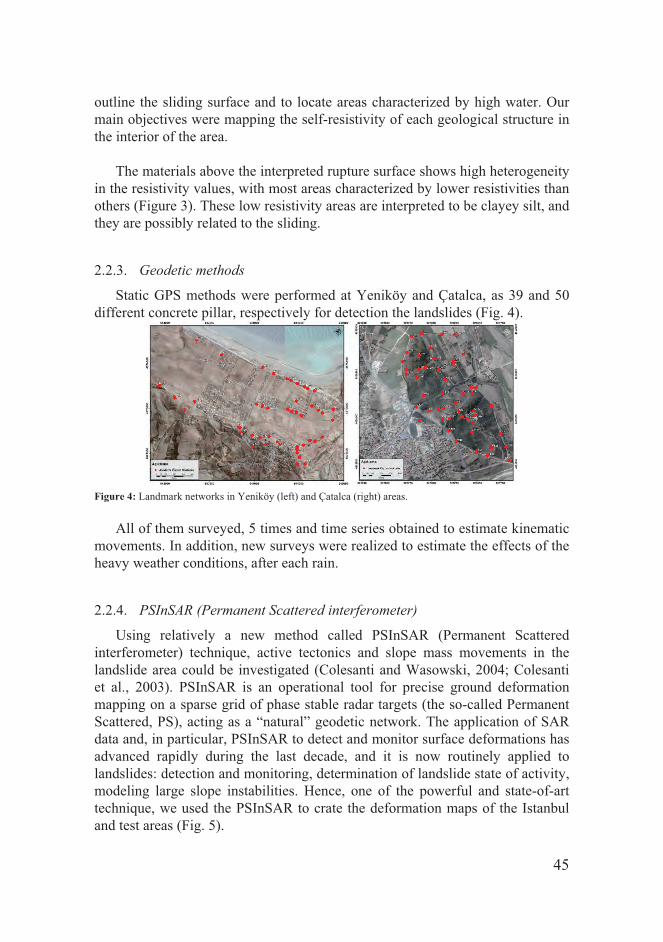
45

outline the sliding surface and to locate areas characterized by high water. Our main objectives were mapping the self-resistivity of each geological structure in the interior of the area.

The materials above the interpreted rupture surface shows high heterogeneity

in the resistivity values, with most areas characterized by lower resistivities than others (Figure 3). These low resistivity areas are interpreted to be clayey silt, and they are possibly related to the sliding.

2.2.3. Geodetic methods

Static GPS methods were performed at Yeniköy and Çatalca, as 39 and 50 different concrete pillar, respectively for detection the landslides (Fig. 4).

Figure 4: Landmark networks in Yeniköy (left) and Çatalca (right) areas.

All of them surveyed, 5 times and time series obtained to estimate kinematic movements. In addition, new surveys were realized to estimate the effects of the heavy weather conditions, after each rain.

2.2.4. PSInSAR (Permanent Scattered interferometer)

Using relatively a new method called PSInSAR (Permanent Scattered interferometer) technique, active tectonics and slope mass movements in the landslide area could be investigated (Colesanti and Wasowski, 2004; Colesanti et al., 2003). PSInSAR is an operational tool for precise ground deformation mapping on a sparse grid of phase stable radar targets (the so-called Permanent Scattered, PS), acting as a “natural” geodetic network. The application of SAR data and, in particular, PSInSAR to detect and monitor surface deformations has advanced rapidly during the last decade, and it is now routinely applied to landslides: detection and monitoring, determination of landslide state of activity, modeling large slope instabilities. Hence, one of the powerful and state-of-art technique, we used the PSInSAR to crate the deformation maps of the Istanbul and test areas (Fig. 5).

46

Figure 5: Permanent Scattered interferometer maps of the Istanbul and project areas.

2.2.5. Application of TDR methods (Time Domain Reflectometer)

Time domain reflectometry (TDR) is a new approach to monitoring landslide and embankment stability. While it is developed to locate breaks and faults in communication and power lines, TDR can be used to monitor the movement of earth slopes (Kane and Beck, 1996). Data collection consists of simply attaching a TDR cable tester to a coaxial cable grouted in a borehole, and taking a reading. An electrical pulse is sent down the coaxial cable. When the pulse encounters a break or deformation in the cable, it is reflected. The reflection shows as a "spike" on the characteristic cable signature (Kane and Parkinson, 1998).

The relative magnitude and rate of displacement and the location of the zone

of deformation can be determined immediately and accurately. The Fig. 6 compares inclinometer readings with TDR signatures from the same location. The size of the spike increase correlates with the magnitude of movement on the ground surface as shown by the inclinometer (Beck and Kane, 1996).

TDR technique is applied as another state-of-art monitoring system for

subsurface deformation (landslide). A TDR measuring system consists of three major elements: The measuring device (TDR cable tester including data logger), the lead cable (low loss coaxial cable), which connects the measuring, cable to the measuring device, and the measuring cable (semi rigid coaxial cable).

47

Figure 6: TDR measurements

TDR can identify and localize discrete deformation zones with high accuracy. When the landslide starts to move in a shear zone, the coaxial cable is deformed, altering the distance between inner and outer conductor of the cable (Fig. 6). This change in the cables geometry can be identified localized and analyzed (O’Conner & Dowding 1999).

2.2.6. Application of inclinometer methods

Inclinometer methods were performed at boreholes in Yeniköy and Çatalca areas at five 10 sites for detection the land-slides (Wash, 1997; Green and Mikkelsen, 1986; Dunnicliff and Mikkelsen, 2000 and ASTM, 1986). At first, the boreholes locations were selected, based on seismic studies. After that, first inclinometer measurements were realized and the borehole geometry was defined, as a function of the depth. Hence, an inclinometer array was established to check the critical level and installed to the borehole for continuous measurements for the sliding at the critical level. All the data transferred online and data evaluation is being performed on a daily basis. Installation and measuring steps of the inclinometer wells are given at Figures 7 and 8.

Figure 7: Flow chart shows the installation of the inclinometers.

INCLINOMETER MEASUREMENTS

Side Selection For Wells

Realizitation of Drilling

Installation of Inklinometer

Case

-Geologic (Core) -Geotechnical (SPT, UD)

-Geologic -Geophysics -Geodetic -Side Observation

Installation of Head of Wells

For measurements

Widening of the Inclinometer-

Wells

48

Figure 8: Flow chart shows the inclinometer measurements.

2.2.7. Multibeam Bathymetry

In addition to the land studies, we focus to the offshore in order to correlate the structural anomalies between land and see, along the coastlines. Therefore, using multibeam technique, depth of the shallow sea-floor (up to 20m depth of water) morphology along the coastal zone (Fig. 9) has been mapped in order to determine the influences of the coastal landslides in the sea-floor (Fig. 9).

Figure 9: Morphologic map of the studied area (at left) and Examples of the influences of the coastal landslides in the sea-floor.

3. EXPECTED AND PRELIMINARY RESULTS AND OUTPUTS

Faults situated in Istanbul Metropolitan Area (Between Büyükçekmece-Küçükçekmece and Tuzla-Kartal), which are suspected to be active, started to be investigated by seismologic/geodesic methods. First results show that eastern part of Istanbul seems activate than east part of Istanbul.

As another main task, methodologies were developed to determine and

monitor landslides by doing multidisciplinary research in priority landslide areas. Research will be realized to determine shallow sea bottom morphology (up to 20m water depth) between Büyükçekmece-Ataköy to reveal sea/land transition zone detail from landslide perspective. Now, continuous data collection runs from the inclinometer and we observe the active deformation as a function of the heavy weather conditions.

Inclinometer Measurements

Test of the Casing Grooves

First, Offline Measurements

Periodic, offline Measurements

Installation of the Inclinometer

Arrays For online measurements

49

During the studies, regional earthquake Information based on scientific

findings obtained by continuous geochemical and microseismological studies of TUBITAK MRC Earth and Marine Sciences Institute transferred to Istanbul Metropolitan Municipality (IMM) and thereby to Directorate of Disaster Coordination Center (AKOM) to provide information for disaster coordination and alert at medium term.

REFERENCE

ASTM (1986). Standard Test Method for Monitoring Ground Movement Using Probe-Type Inclinometers. ASTM D6230-98. Annual Book of ASTM Standards, Vol. 04.09, ASTM International, West Conshohocken, Pa.,

Beck, T. J., and Kane, W. F. (1996). "Current and Potential Uses of Time Domain Reflectometry for Geotechnical Monitoring." Proceedings, 47th Highway Geology Symposium, Cody, WY., Wyoming Department of Transportation, 94-103.

Colesanti, C.; Ferretti, A.; Novali, F.; Prati, C.; Rocca, F. (2003) SAR monitoring of progressive and seasonal ground deformation using the Permanent Scatterers Techniques. IEEE Trans. Geosci. Remote Sens. 41, 1685-1701.

Colesanti, C.; Wasowski, J. (2004) Satellite SAR interferometry for wide-area slope hazard detection and site-specific monitoring of slow landslides. Proc. Ninth Int. Symp. Landslides, Rio de Janeiro, Brazil, pp. 795-802.

Dobrin. M. B., (1976), Introduction to geophysical prospecting: McGraw-Hill Book Co. Dunnicliff, J., and P. E. Mikkelsen (2000). Overcoming Buoyancy During Installation of

Inclinometer Casing. Geotechnical News Magazine, Vol. 18, No, 3, pp. 19–20. Green, G. E., and P. E. Mikkelsen (1986), Measurement of Ground Movement with Inclinometers.

Proc., 4th International Geotechnical Seminar, Field Instrumentation, and In Situ Measurements, Nanyang Technical Institute, Singapore, pp. 235–246.

Kane, W. F. and Parkinson, W. A. (1998). "Remote Landslide Monitoring Including Time Domain Reflectometry." Training Manual, KANE GeoTech, Inc., Stockton.

Kane, W. F., and Beck, T. J. (1996). "An Alternative Monitoring System for Unstable Slopes." AEG NEWS, Association of Engineering Geologists, 39 (3), 24-26.

O’Connor, K. M., Dowding, Ch. H. (1999), GeoMeasurements by Pulsing TDR Cables and Probes. Boca Raton: CRC Press.

Sheriff, R. E., (1978), A first course in geophysical exploration and interpretation: International Human Resources Devel. Corp.

Telford, W. M., Geldart, L. P., Sheriff. R. E., and Keys, D. A., (1976), Applied geophysics: Cambridge University Press.

Wash.M., (1997), Slope Indicator Company. QC Inclinometer Casing Installation Guide, 27 pp.

50

SISMOKUL - SCHOOL SEISMOLOGY

MEHMET ERG N TUBITAK Marmara Research Center (MRC)

Earth and Marine Sciences Institute Gebze-Kocaeli-Turkey

mehmet.ergin@mam.gov.tr

Abstract

SISMOKUL (School Seismology) is an experimental and practical training program, which combines physics and earth sciences by means of seismological research for middle and high school students across the country. This educational program focuses on education on seismic risk through a scientific and technological approach. SISMOKUL is a national education outreach project, based out of TUBITAK MRC Earth and Marine Sciences Institute (EMSI), that will established a network of seismic recording stations at high schools across the Turkey. Seismometers measure the ground motions of all types including those generated by near and distant earthquakes. Students in the SISMOKUL program are given the opportunity to explore the Earth's interior through seismic data obtained from their classroom seismometers. Students use the SISMOKUL network to study earthquakes, build research skills and improve their understanding of the planet Earth.

Keywords: Seismology, school education, and earthquakes

1. WHAT IS SISMOKUL (School Seismology)

It is well-known that Turkey is situated on an active seismic zone. Destructive earthquakes have occurred historically as well as in the recent past. Many regions of Turkey can expect earthquakes in the future as severe as in the

51

past as demonstrated by the existing evidence and deposits throughout the country.

Increasing our knowledge about the cause of earthquakes and its effect on people in areas with high seismic risk through educational awareness programs is an important step in the direction of earthquake risk reduction. Promoting earthquake awareness is an important contribution toward the prevention of fatalities and injuries.

SISMOKUL is an experimental and practical training program, which combines physics and earth sciences using seismological research. It is geared toward middle and high school aged students across the country and focuses on education about seismic risk utilizing a scientific, technological approach.

The seismology in Schools concept started in the United States 15 years ago as the Princeton Earth Physics Project (PEPP) at Princeton University. From this the program was expected and it soon become highly successful program currently operated by the Incorporated Research Institution for Seismology (IRIS) organization. Within the last decadey U.K, France, Germany, Italy and Switzerland also launched an equivalent initiative, through the research institutes and universities. TUB TAK-MRC EMSI has introduced the SISMOKUL Project in response to the increasing interest by students in earthquakes, and Earth Sciences in general. This is accomplished by installing seismological station in school in order to record seismic activity in real time. SISMOKUL was first launched one year ago at Doga College in Istanbul and the aim is to expand it to another school in other cities in the next two years.

2. GOAL of SISMOKUL

The main goals of this program are: Constitute a nationwide educational outreach program that combines state-

of-the-art seismological research with hands-on classroom training for middle and high school students in the physical and earth sciences.

To make possible for the secondary school community to learn about instrumental measurements, utilizing environmental scientific data parameters. This program will introduce them to seismological science in preparation for the future.

To improve educational opportunities for students in the earth sciences field in order to help them learn what it is, how to observe and how it functions.

To enrich science education by bringing technology into the classroom while fostering cooperation between research universities and secondary educational institutions. SISMOKUL will engage teachers and students to acquire knowledge while studying seismological data from SSMOKUL seismometers installed at their schools. It will help teachers bring inquiry-based methodology

52

for the teaching of science in classroom. It will provide hands-on activities and real data for scientific investigations

3. CONTRIBUTION TO THE SCHOOL CURRICULUM

The school curriculum has several important aspects (placing large emphasis

on new communication technologies): • scientific content (instrumentation, geophysics, Earth sciences), • educational dimension (sensitization to seismic risk) • regional, national and international dimension (networking several

schools) Within the framework of courses in Earth and Life Sciences, Physics,

Technology and Geography, there are various pedagogical suggestions for the curricula of schools on the following themes: measurement of a parameter, measure of one’s geological environment, complex mechanisms and notion of environmental risks.

4. OUTCOMES

The SISMOKUL project enables schools to detect signals from large earthquakes happening anywhere in the world. The sheer destructive power of earthquakes has always held a fascination for students children. This project capitalizes on this natural interest by making use of earthquakes and seismology as a unifying theme to teach a range of basic science concepts • detect world earthquakes in the classroom using a simple seismometer

system • exchange earthquake data with schools around the world • use seismology to teach geography and physics lessons with

classroom resources developed with project members Operating seismic stations will raise awareness of the worldwide earthquake

activity, earthquake locations and frequencies. Students will be encouraged to ‘think outside the box’ and expand their horizons.

Students will encourage the school community to develop relationships with other schools helping the teachers to increase, to expand and to share pedagogical interests.

Management of seismological stations at schools can be starting point for scientific workshop. In such a case, students would have the responsibility of managing a seismological station. The network of seismological stations and its database can also be springboard for multidisciplinary projects bringing together teachers of experimental sciences, technology, mathematics and geography.

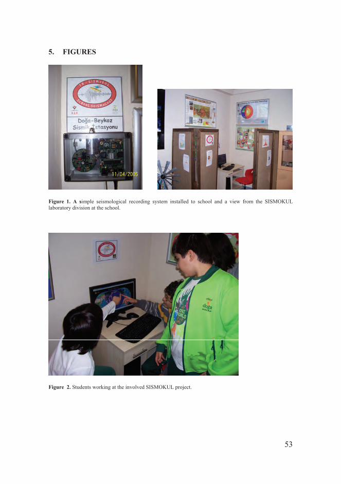
53

5. FIGURES

Figure 1. A simple seismological recording system installed to school and a view from the SISMOKUL laboratory division at the school.

Figure 2. Students working at the involved SISMOKUL project.

54

EVOLUTION OF METHODOLOGY MULTI-PARAMETRICAL

OBSERVATION ON THE TERRITORY OF GEORGIA

NINO KAPANADZE, GEORGE MELIKADZE, ZURAB MACHAIDZE, SHOTA KIMOTIDZE, KHATUNA BEDIANISHVILI

M. Nodia Institute of Geophysics, Iv. Javakhishvili Tbilisi State University

Abstract

Since 1979, researches for earthquake forecasting promoted development of a hydro-chemical network of special regime regional observation. On the territory of Georgia hydro-chemical observations are carried out on 23 boreholes. During observations a lot of anomalies were fixed, but because of the diversity of chemical water content it was impossible to conduct observations of the unified parameters for creating the complete picture of strains on the whole territory. This is the reason why we decided to conduct observations for those parameters which could fix tidal variations with deformation of 10-8 degree, what is compared with strains differences during earthquakes preparation period. Besides, it was possible to conduct unified observations. Water level in the deep boreholes was one of them. That way since 1885, the network of 10 boreholes of different depth (from 250 up to 3500 m) covers the whole territory of Georgia. Boreholes characterize all basic geo-plates and open waters of deep aquifer, actually they represent sensitive volumetric strainmeters, and react on the deformations about 10-7 -10-8, caused both by endogenous, and exogenous factors. A borehole was considered informative if it was fixing tidal variations and was included in the network. Special monitoring equipment is installed at boreholes which record several parameters, i.e. water level and micro-temperature, atmosphere pressure and surface temperature, tilt, magnetic field and others. The data can be gathered in real time using the GSM net.

Keywords: Multi-parameters, network.

1. Introduction

Georgia is a part of a big geodynamical active region. As a result of plate migration, strong compressive strains are being built in the crust.

55

The energy released during sudden stress drop events may trigger earthquakes.

All over the world and in Georgia also, various anomalies (Hydro-dynamical, hydro-chemical, micro-temperature etc) are observed before earthquakes, besides in most cases, on enough distant places from epicentres. Therefore studying the geodynamical processes may help to forecast the natural catastrophes with reasonable probability.

2. Regional Geography and Geology

Georgia is a country in the Caucasus region of Eurasia. Situated at the juncture of Western and Eastern Asia. To the west it is bounded by the Black Sea, to the north - by Russia, to the south - by Turkey and Armenia, and to the east - by Azerbaijan. Georgia covers a territory of 69,700 km². The climate in Georgia varies significantly, and ranges from subtropical conditions on the Black Sea coast to continental with cold winters and hot summers in the east. The cold air from the north is prevented by the Greater Caucasus range. On the other hand, warm and moist air from the Black sea moves into the coastal lowlands, where the annual precipitation ranges between 1000 and 2000 mm, often exceeds 2000 mm on the coast, whereas the eastern part receives precipitation between 400 and 1600 mm during spring and autumn. The mean temperature in winter is 5 °C and in summer 22 °C Geologically, the territory of Georgia is located in the Central and Western parts of the Transcaucasus and lies between the Eurasian and Afro-Arabian plates. The geologic evolution of Georgia is controlled, to a great extent, by the development of the whole Caucasus segment of the Mediterranean belt. Three major tectonic units can be distinguished according to the geologic evolution of Georgia: 1) Fold system of the Greater Caucasus which represents a marginal sea in the geological past, 2) Transcaucasian intermountain area which marks the northern part of the Transcaucasian island arc, 3) Fold system of the Lesser Caucasus, the southern part of the ancient Transcaucasian island arc.

2.1. HYDROCEMICAL MONITORING

Since 1979, the researches for the forecast of earthquakes promoted development of a hydro-chemical network of special regime regional observation. On the territory of Georgia hydro-chemical observations are carried out on the 23 boreholes (Fig. 1).

56

Fig.1. Scheme of hydro-chemical monitoring stations on the territory of Georgia

Measurements of water debit- by volumetric method, temperature of

water and air - by mercury thermometer were daily carried out on the water points. Helium concentration was directly defined on the water points with the same frequency. Chemical composition of water was assessed on 20 components (HCO3, Cl, SO4, Na, K, Ca, Mg, J, Br-, Zn, Cu, Fe, Mn, He etc). Water chemical analysis was done by standard methodology.

The only way in the absence of criteria of estimation of information values was to make retrospective analysis on energy of occurred earthquakes (Fig. 2).

During observations a lot of anomalies were fixed, but because of the diversity of chemical water content it was impossible to conduct observations of the unified parameters for creating the complete picture of strains on the whole territory (Melikadze G., Adamchuk Y., et al., 1989).

This is the reason why was taken a decision to conduct observations for those parameters which could fix tidal variations with deformation of 10-8

degree, what is compared with strains differences during earthquakes preparation period. Besides it was possible to conduct unified observations. The water level in the deep boreholes was such a parameter (Hsieh et al., 1987, Hsieh et al., 1988).

57

Fig. 2 Variation of hydro-chemical parameters and earthquakes energy at the Skuri, Tsinubani and Tiniskhidi stations

Skuri

0

100

200

300

400

500

600

20/12/1981 08/02/1982 30/03/1982 19/05/1982 08/07/1982 27/08/1982 16/10/1982 05/12/1982 24/01/1983 15/03/1983 Data

Na, Ca- mg/l

0

2

4

6

8

10

12

14

16Energy

Na Ca energy

Tiniskhidi

9200

9300

9400

9500

9600

9700

9800

9900

10000

10100

10200

12/08/1981 01/09/1981 21/09/1981 11/10/1981 31/10/1981 20/11/1981

Data

Cl

0.0000

0.0010

0.0020

0.0030

0.0040

0.0050

0.0060

0.0070Energy

Cl energy

Tsinubani

4

5

6

7

8

9

10

11

10/06/1983 30/06/1983 20/07/1983 09/08/1983 29/08/1983 18/09/1983

Data

Cl, pH

0.00

0.05

0.10

0.15

0.20

0.25

0.30

0.35

0.40Energy

Cl PH energy

58

2.2. WATER LEVEL VARIATION MONITORING IN THE BOREHOLES

The modern methods of earthquakes forecast allow watching temporal and spatial changes of strain in the terrestrial crust. One of them is the monitoring method of hydrogeodeformation ground field (HGF). A regime network, according to the development of VSEGINGEO, in Caucasus has been established since 1985. Till now the network of 10 boreholes of different depth (from 250 up to 3500 m) covers the whole territory of Georgia. Boreholes characterize all basic geo-plates and open waters of deep aquifer, actually they represent sensitive volumetric strainmeters, and react on the deformations about 10-7 -10-8, caused both by endogenous, and exogenous factors. A borehole was considered informative if it was fixing tidal variations and was included in the network (Melikadze G. et al., 1989).

They are situated in different tectonic areas. The deep boreholes with undisturbed regime were chosen for the observations which were not influenced by other boreholes.

Boreholes are equally spread all over the territory, basically on main geo-plates. These wells record all kinds of deformation caused by exogenous (atmospheric pressure, tidal variations and precipitation), as well as endogenous\ tectonic processes (Rojstaczer S. et al., 1998, Melikadze et al., 2002). On some boreholes, reaction of tidal-variation or atmosphere pressure dominated. For example, the atmospheric pressure is dominant at Adjameti and Oni boreholes and then tidal variations. But the tides are dominant on the Marneuli and Lagodekhi boreholes (Melikadze et al, 2004).

Distinctions in dominating factors are caused by depth of a borehole, its design, originality of a geological and hydro-geological structure water aquifer, value of the gas factor, etc.

For the conductance of qualitative observations appropriate equipment is necessary which could ensure frequent parameters inquiry, data transmission of determined frequency. After searching we have chosen data logger by American production to which 8 analogue ports and one pulse port are attached as well as corresponding sensors of water level or water pressure, atmospheric pressure and temperature.

This equipment ensures attachment of other informative sensors, which were chosen for such observation as magnetic and tiltmeter, Radon and Helium gases. The registration of this data occurs with a frequency of one time in a minute.

59

Fig. 5 Variations in time of water level (the bottom line), atmospheric pressure (the top line) and the tides (an average line) in the Adjameti borehole. Vertical lines correspond to the occurrence of earthquakes.

.

Fig. 6. Variations in time of water level (the bottom line), an atmospheric pressure (the top line) and the tides (an average line) in the Oni borehole. Vertical lines correspond to the occurrence of earthquakes.

Fig. 7 Variations in time of water level (the bottom line), atmospheric pressure (the top line) and the tides (an average line) in the Marneuli borehole. Vertical lines correspond to the occurrence of earthquakes.

60

The data collection takes place with a frequency of one time in a day or more

rarely. The data reception is ensured with the help of software of American data-logger.

All the data is collected in Matlab for the following processing, water level, atmospheric pressure, temperature, tilt-meter, which we get from the boreholes, tidal variations, which we calculate from the special program (GRAV To) and earthquakes data, which we receive from seismic station. In Matlab we calculate the stress condition from the earthquakes data, for each borehole by Dobrovolsky's e=10 1, 3M-8, 19/R3 equation.

2.3. MICROTEMPERATURE MONITORING

Since 1999, authors with German colleagues have been carrying out researches at Tbilisi hydrothermal field in Eastern Georgia to study hydrodynamical and microtemperarture precursors of earthquakes.

Has been analyzed the long-time period materials; which was kept for today and give them possibility to find out relations between microteperature and hydrodynamic variation and tectonic motion and to define the short-term precursors of earthquakes.

2.3.1. Equipment

In order to achieve the objectives of the present research the innovative equipment (Buntebarth, 1999) was tested and installed in boreholes in THF. The devices are able to record very weak water migrations in the subsurface either by high-precision temperature measurements or by combined temperature and water level records. As far as the equipment operates in autonomous mode with energy saving electronics it can record data for several weeks or months depending on the reading frequency when using three alkaline batteries of size D. The regime observations of on the level, pressure and microtemperatures were organized at boreholes, located on Saburtalo (Lisi) and Tbilisi Central hydrothermal areas as well as at Sartichala-Teleti oil field (Fig. 4).

Temperature and water level data were recorded in boreholes with accuracy 0.5 microKelvin and 0.1cm correspondingly at a frequency of 10 or 20 min at the depths of the order of 200 m.

After selecting 9 boreholes the equipment was installed in some of them.

2.3.2. Data analysis

The temperature regime of underground waters shows the hydrothermal

processes in the earth crust that is influenced by movement of thermal waters.

61 61

Stress/strain variations in the crust produce the changes in the local strain field as well as pressure of water, saturating pore and cracks system. Movement of stationary heat flow occurs through pore system as well. That’s why microtemperature changes are observed– anomalies coupled with stress/strain variations.

According to got data influence of season variations effects differently on the water level in the nearby located different boreholes. Water temperature changes by increasing depth and it means that there is close connection between water level and its temperature variations. And this connection is closer in the deep wells, where the influence of atmospheric pressure is excluded.

25 April 2002 the significant earthquake (M = 4.5) occured in the centre of Tbilisi that causes damage, assessed as 200 mln USD. The EQ was preceded by two foreshocks at 11 and 20 of April. Duration of shaking was 3 s. Observed macroseismic intensity was 6-7 in the epicentral area and the maximal horizontal acceleration was 0.11 g at the distance 8 km from epicenter. The EQ was followed by aftershocks, some of them with intensity 3.

Tbilisi 2002

0

100

200

300

400

500

600

700

800

900

12.29.01 01.28.02 02.27.02 03.29.02 04.28.02 05.28.02 06.27.02 07.27.02 Date

Bot. Gar. Water level (cm)

-100

0

100

200

300

400

500

600

700

Varketili Water level (cm)

Botanic Varketili

8.1-

15

7-50 10

.5-1

5

8-20 12

.2- 5

7.8-

15

K - Earthquake - Distance

7-65-12

Fig. 6 Water level changes in Varketili and Botanic garden boreholes in 2002

Unfortunately, the water level equipment was not operating during that event (see Fig. 6), but on the other hand we observe very impressive microtemperature (microT) anomaly at Varkertili well before that EQ (Fig. 4). The epicentral distance was around 3 km. The anomaly is expressed as a strong scatter of temperatures around the background values and is evident at all three levels of recording: 150, 200 and 250 m. Deviations began at the 150 m-level on 5 April 5.00 and on deeper levels on 6 April, 00.00 that is 50 days before mainshock and 36 days before the first foreshock. The scatter was in the range 0.970, 0.01 and 0.025 Mk on the levels 150, 200 and 250 m respectively with predominant tendency to lower temperature values. After the anomalous period, which lasts 12-13 days, the mT values return to their background level and stay close to the old baseline for 6-7 days that is till the EQ of 25 April occurs.

61

62 62

Sensor I

-5

0

5

10

15

20

25

30

35

1.1.02 1.31.02 3.2.02 4.1.02 5.1.02 5.31.02 6.30.02 7.30.02 8.29.02

Date

Temperature mK

0

5

10

15

20

25St.dev mK

Temperature mK K -Earthquakes Distance St.dev mK Sensor II

-5

0

5

10

15

20

25

30

35

1.1.02 1.31.02 3.2.02 4.1.02 5.1.02 5.31.02 6.30.02 7.30.02 8.29.02

Date

Temperature mK

0

5

10

15

20

25St.dev mK

Temperature mK K -Earthquakes Distance St.dev mK

Sensor III

-5

0

5

10

15

20

25

30

35

1.1.02 1.31.02 3.2.02 4.1.02 5.1.02 5.31.02 6.30.02 7.30.02 8.29.02

Date

Temperature mK

0

5

10

15

20

25St.dev mK

Temperature mK K -Earthquakes Distance St.dev mK

Fig 8. Time series of microtemperatures (upper curves) and standard deviations of T (lower curves) before, during and after the Tbilisi earthquake 25 April 2002 (M=4.5) at Varketili well, which is situated 3 km apart from the epicenter. Sensors I, II and III are deployed at depths 100, 150 and 200m accordingly.

The main event was marked by the post-seismic temperature step-like increase by 1 mK, 0.3 mK and 1 mK for sensors at 250, 200 and 150 m respectively. The microT-step lag relatively to the moment of the EQ was of order of 14 hours. Analysis of data of Fig. 15 shows that the strong microT anomaly originates a week before the first foreshock and finishes two days before the second foreshock; we cannot see any clear immediate responses to the foreshocks or to the main shock. This entire means that the connection between microT anomalies and tectonic/seismic events is quite complicated and different hydraulic effects can both precede seismic events and lag after them.

We could mention here the water level anomalies that can be related to 25 April events (Fig.14), though the anomalies in WL are not so clear due to technical reasons. At the Varketili well the strong increase of WL level (50 cm) began in August-October that is 7 months before the EQ;

63

Considering Figs 8 and 9 and taking we can conclude that the rise of seismic activity in Tbilisi area in the spring 2002 could be predicted if there were telemetric system for operative transmission of data and corresponding operative proceeding centre, because clear pre-seismic effects were observed in various geophysical and geochemical fields (Figs.6-9)

0

500

1000

1500

2000

2500

3000

3500

4000

4500

5000

5/ 29/

01

7/ 8/ 0

1

8/ 17/

01

9/ 26/

01

11/ 5/

01

12/ 15

/ 01

1/ 24/

02

3/ 5/ 0

2

4/ 14/

02

5/ 24/

02

7/ 3/ 0

2

8/ 12/

02

9/ 21/

02

10/ 31

/ 02

0

50

100

150

200

250

300

350

mamkoda

foniW

botan

vake

delisi

Fig.4. Radon concentration change before Tbilisi earthquake 25.04.02

3. Hydrodynamical observation station Site selection is an important moment in deploying the hydrodynamic

observation network. There are wells, which are more sensitive to the strain than others. The same is related to the depth of observations: the strain-sensitivity in the same well is different at different level.

In principle, the ideal hydrodynamic observation station should provide monitoring of following parameters:

1. Atmospheric pressure 2. Precipitation, snowfall and snowmelt 3. Air (surface) temperature 4. Tecnogenic impact 5. Aquifer characteristics (storetility, transmissivity, hydraulic conductivity,

screened area, drained and undrained poroelastic parameters, gas phase content) 6. Seismic catalogue of strong and near events 7. Strains (Tides, tectonic movements, slow earthquakes) 8. Water level 9. Water temperature at various depths (temperature gradient) 10. Water conductivity in the borehole 11. Water chemistry 12. Rn concentration variation 13. Electromagnetic field anomalies

64

Such integrated observations could provide for quantitative interpretation of observed anomalies. It is obligatory to have most of this data in order to give at least reasonable qualitative conclusions.

4. Conclusion

According to the new methodology, we have selected informatively deep boreholes for the special network, which covers the whole territory of Georgia and characterizes all basic geo-plates. They represent sensitive strainmeters and fix the deformations processes about 10-7 -10-8, caused both by endogenous and exogenous factors.

All over the world including Georgia, various anomalies (Hydro-dynamical, hydro-chemical, micro-temperature etc) are observed before earthquakes, besides in most cases, on enough distant places from epicentres. Therefore, studying the geodynamical processes may help to forecast the natural catastrophes with reasonable probability.

Analyzing data of different parameters show us the importance of improving the existing multiparametric observation network by adding new parameters as well as to expansion of contacts and collaboration with colleagues from our neighbouring countries in order to exchange data and to create the observation network on the territory of whole Caucasus and Black Sea region.

References

Hsieh, P. A., I. D. Bredehoeft, S. A. Rojstaczer. Response of Well-Aquifer Systems to Earth Ties: Problems Revisited. Water resources Research vol. 24. No. 3. 1988, p.p. 468-472. Melikadze, G., Popov E. A. Technique of Hydro-geological supervision with the purposes of the forecast earthquake on territory of Georgia. A series geology «Gruziinti» N7, 1989. Rojstaczer, S. 1988. Intermediate period response of water wells to crustal strain: Sensitivity and noise level, J. Geophys. Res., 93, 13,387-12,402. Melikadze G., Matcharashvili T., Chelidze T., Ghlonti E. Earthquake related disturbance in stationarity of water level variation. Bulletin of the Academy of sciences of the Georgian, 165 &#8470; 1, 2002 Melikadze G., Buntebarth G., Chelidze T. Hydrodynamic and

microtemperature monitoring in seismic areas. Georgian Engineering News, # 3, 2004 , p.p 12-132

65

NEW METHOD OF HYDRODYNAMICAL DATA ANALYSIS

GENADI KOBZEV, GEORGE MELIKADZE, TAMAR JIMSHELADZE

M. Nodia Institute of Geophysics, Iv. Javakhishvili Tbilisi State University

Abstract

Revealing mechanism of interrelation between the deformation processes, strong earthquakes and hydrodynamics of underground waters would allow explaining precursory behaviour of hydrodynamic field and developing scientifically well grounded methods of earthquakes’ forecast. We have developed a new method using computer program MatLab. It enables to synthesize a theoretical signal and compare it with original data of water level. The program enables to characterize each exogenous parameter separately. It allows studying the influence of each of them on the aquifer. It is determined that the aquifers are influenced by all kinds of exogenous factors. The reaction of boreholes demonstrates that one of them can dominate. After processing by suggested method almost identical figures describing the tectonic factor have been received. Keywords: exogenous factors, earthquakes’ forecast.

1. Introduction Revealing mechanism of interrelation between the deformation

processes, strong earthquakes and hydrodynamics of underground waters would allow explaining precursory behaviour of hydrodynamic field and developing scientifically well grounded methods of earthquakes’ forecast. At the analysis of materials, scientists individually selected methods of mathematical statistics, but all of them had one thing in common: after removal of the trend caused by exogenous factors (tidal variation and atmospheric pressure) they used frequency filters (P. A. Hsieh at al, 1987, 1988), that in our opinion, distort required endogenous signal. The residual values were analyzed for revealing correlation of water level variations with seismic events. Our method, which uses the computer program MatLab, created exogenous theoretical signal and compare it with real signal. In comparison with the last, enables to characterize every exogenous

66

parameter separately. That makes possible to study influence of each of them on the water aquifer. 2. Data analysis

The following factors influence the aquifer and change water level: tidal, atmospheric pressure, precipitation, tectonic-seismic factors, the error from apparatus and so on. Let us represent the summary signal using linear equation:

Water level = a*tidal+ b*atmos+c*precip + e;

Where a- is coefficient for tidal variation, b–atmosphere pressure, c–precipitation e–geodynamical signal.

Water level and atmospheric pressure are measured directly at boreholes. Theoretical data for tidal variations are generated by the program GRAV. To determine the, stress conditions in the aquifer after strong earthquake, Dobrovolsky's e=10 1, 3M-8, 19/R3 equation has been applied.

Fig. 1. Water level, tidal variation, atmosphere pressure and earthquakes at Marneuli station Upper line is water level, lower line is tidal variation, middle line is atmospheric

pressure. Vertical lines are earthquakes. In the catalog we select earthquakes, which are strong enough to affect boreholes’ sites (Fig. 1). We can also select earthquakes by magnitude and distance from the borehole.

Program finds minimums time-points of tidal variation and compare it with water level variation value’s point at the same time. By connection of these

67

points we receive some “trends” of both parameters. After extracting this “trend” from the original data, we receive “residual” values of water level variation. Program calculated such type of “residual” values for atmosphere pressure, also.

Fig. 2 “Residuals” line after extraction of “trend”

Program allows extracting differently influence of tidal-variation, atmosphere pressure and both totally.

Fig. 3. Water level variation after extraction of tidal variation (upper line), atmosphere

pressure (middle line) and of both parameters (lower line).

68

Correlations between parameters (water and tidal; water level and atmosphere pressure; water level and tidal variation + atmosphere pressure) can be calculated.

Fig. 4. Variation of Coefficient correlations between of water level and tidal variation. Vertical strait line is earthquakes.

In order to find disturbances of environment’s equilibrium condition

in relation to the exogenous factors, caused by imposing an additional endogenous component (Melikadze G. at al., 1989, 2002), special program had been developed, allowing to find components of this equation.

water level(x)=a*tidal(x)+b*atmosphere(x)+c.

During monitoring we measure water level, tidal variation and atmospheric pressure. In order to find coefficients a, b, c it is necessary to write a system of 3 (or more) equations. MatLab allows working with over-defined systems and the whole time interval will be split on many intervals (for example on 24 hour’s intervals). For every interval the program finds a set of coefficients. During calculations the following equation are solved, where W(x) is water level variation, T(x) is tidal variation; A(x) is atmospheric pressure, is constant. Program use measured values of W, A, T at the moment xi for system of equations

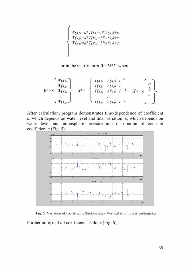
69

or in the matrix form W=M*X, where

After calculation, program demonstrates time-dependence of coefficient a, which depends on water level and tidal variation, b, which depends on water level and atmosphere pressure and distribution of constant coefficient c (Fig. 5).

Fig. 5. Variation of coefficients (broken line). Vertical strait line is earthquakes.

Furthermore, c of all coefficients is done (Fig. 6).

W(x1)=a*T(x1)+b*A(x1)+c W(x2)=a*T(x2)+b*A(x2)+c W(x3)=a*T(x3)+b*A(x3)+c

W(x1)W(x2)W(x3) … W(xn)

W = M =

T(x1) A(x1) 1 T(x2) A(x2) 1 T(x3) A(x3) 1

… T(xn) A(xn) 1

X= a b c

70

Fig. 6. Spectral graphics of every coefficients.

Program calculates “summary” signal (Fig. 7), which demonstrate reliability and relation of anomalies for all coefficients.

Fig. 7. Variation of “summery” signal (broken line). Vertical strait line is earthquakes

Results of data analysis have shown deterioration of reaction of

coefficients a, b, c before and during seismic event that demonstrates the informatively of water level as an indicator of tectonic activity.

71

3. Conclusion

Water level variation basically is caused by the atmospheric

pressure and earth crust tide variations, as well as the “background” values, which change during earthquake preparation period. Amplitude and period of a, b, c coefficient changed by energy of earthquakes. References P. A. Hsieh, I. D. Bredehoeft, I. M. Farr. Determination of Aquifer Transmissivity from Earth Tide Analysis. Water resources research. vol. 23. 10. 1987, p.p. 1824-1832. P. A. Hsieh, I. D. Bredehoeft, S. A. Rojstaczer. Response of Well-Aquifer Systems to Earth Ties: Problems Revisited. Water resources Research vol. 24. No. 3. 1988, p.p. 468-472. Melikadze G., Popov E. A technique of Hydro-geological supervision with the purposes of the forecast earthquake on territory of Georgia. A series geology «Gruziinti» N7, 1989. Melikadze G., Matcharashvili T., Chelidze T., Ghlonti E. Earthquake related disturbance in stationarity of water level variation. Bulletin of the Academy of sciences of the Georgian, 165 &#8470; 1, 2002

72

APPLICATION OF DFA METHOD TO MAGNETIC FIELD DATA

M. CHAMATI 1, P. NENOVSKI 1, M. VELLANTE 2 , U.VILLANTE 2 , K. SCHWINGENSCUH 3 ,

M. BOUDJADA 3 ,V. WESZTERGOM 4

1National Institute of Geophysics, Geodesy and Geography, Bulgarian Academy of Sciences, 1113 Sofia, Bulgaria, 2Department of Physics, University of L’Aquila, L’Aquila, Italy,

3Space Research Institute, Graz, Austria. 4Geodetic and Geophysical Research Institute, Hungarian Academy of Sciences. Sopron, Hungary

Abstract. The detrended fluctuation analysis (DFA) is a method for determining the statistical self-affinity of a signal in stochastic processes and time series analysis. It is very useful in revealing the extent of long-range correlations in time. We apply this method to the analysis of magnetic field data (ULF frequency range) from SEGMA array – a network of magnetic stations geographically located in Italy, Hungary and Bulgaria. We study the behavior of the DFA index, which characterizes the long-range correlations in magnetic field data series over a time period from June 2004 till February 2005. The DFA scaling exponent for each station is computed for two different time scales: 10-180 s and 10-900 s. Our results show both regional trends and local peculiarities of the DFA index. The regional trends are obviously associated with geomagnetic activity (Kp index). The local peculiarities (at a single station) can be produced by multiple sources, may be processes of similar characteristics of limited extent either in the atmosphere/ionosphere system or in the lithosphere.

Keywords: geomagnetic activity, DFA method, SEGMA array.

1. Introduction

Ultra low frequency (ULF) signals may be produced as a result of the interplay of different signals, such as natural signals emanating from solar-terrestrial interaction, lithosphere or artificially generated (industrial noise, disturbances emitted from measurement equipment). In many cases ULF emissions are associated to magnetospheric origin (Masci 2010). To identify the source of ULF emissions associated to the variations of the geomagnetic field different methods (Telesca & Lapenna 2005), such as fractal (Gotoh et al. 1999; Masashi

73

Hayakawa et al. 1999), and multifractal analysis, as well as detrended fluctuation analysis (DFA) (Kantelhardt et al. 2002; Chamati et al. 2009) were applied to geomagnetic data. Despite their differences these methods aim at studying the fractal dimension evolution of time series. In this study we apply the DFA method to identify ULF signatures of series of earthquakes occurred in the Adriatic region in the period June 2004 − February 2005. ULF magnetic field measurements are provided by the SEGMA array and span a longer period than that considered in Ref. (Chamati et al. 2009). SEGMA is a low-latitude magnetometer array in South Europe which consists of three stations in Italy and one in Hungary, latitudinally equispaced between L=1.57 - 1.89 (L is the Mcllwain parameter). Each station is equipped with high sensitivity (~10 pT) triaxial fluxgate magnetometers recording northward (H), eastward (D) and vertically (Z) components of the geomagnetic field variations. An automatic acquisition system collects the data at 1 second interval with timing provided via GPS. Coordinates of all stations are given in (Villante et al. 2006).

2. DFA method

DFA is a well-established method for determining data scaling behavior in the presence of possible trends without knowing their origin and shape (Kantelhardt et al. 2002). In difference to conventional methods, e.g. power spectrum analysis, the DFA permits detection of intrinsic dynamical features, e.g. long-range correlations, embedded in non-stationary time series and avoids spurious detection of apparent scaling, which may be an artifact of non-stationary time series (Buldyrev et al. 1995; Peng et al. 1995). For long-range correlated signals the power spectral density would behave as a power-law of the frequency, thus its slope should be constant and usually denoted by β index.

For the sake of completeness here we give a short description of the method. Consider a time series x(i), where i = 1,2,…N and N is the length of series. First we define the profile of the series x(i) via

=

−=i

kavexkxiy

1])([)( ,

where we have introduced the mean value =

= N

kNave kxx1

1 )( .

Next, we choose a time scale s and divide the profile into Ns = int(N/s) non-overlapping segments of equal length s . Since the length N of the series is often not a multiple of s, a short part at the end of the profile y(i) may remain. In order not to miss this part of the series, the same procedure is repeated starting from the opposite end. Thereby, 2 Ns segments are obtained altogether. The local trend for each of the 2 Ns segments is calculated by a least square fit of the series. Then we determine the variance

74

=

−+−=s

iiyisy

ssF

1

22 )}(])1[({1),( ννν

for each segment ν, ν = 1,…, Ns and

=

−+−−=s

is iyisNNy

ssF

1

22 )}(])([{1),( ννν

for ν, ν = Ns+1,…, 2 Ns. Here, yν(i) is the fitting line in segment ν. After averaging over all segments we derive the following fluctuation function:

2/12

1

2 ]),([2

1)(=

=sN

s

sFN

sFν

ν .

Repeating this procedure for several time scales, F(s) is expected to increase with increasing s. And analyzing log-log plots F(s) vs s the scaling behavior of the fluctuation function will be determined. If the series x(i) is long-range power–law correlated, the fluctuation function F(s) will increase for large values of s as a power-law:

αssF ≈)( .

By applying standard spectral analysis techniques to the series x(i), the power spectra, i.e. the square of the Fourier transform amplitudes for x(i), yields β = 2α −1. The value of α (i.e. the DFA scaling exponent) resulting from a least-square fit to a straight line, reveals the presence, or not, of long-range correlations. In particular, the case α = ½ represents the absence of long-range correlations.

3. Analysis and discussion

We analyzed data from flux-gate magnetometers from 01 June 2004 – 28 February 2005. To this end we extract the nighttime period from 00:00 – 01:00 (UT). At midnight ionospheric activity is at its lowest level. The DFA scaling parameter was determined for two time intervals: 10 − 900 seconds and 10− 180 seconds for vertical (Z) and horizontal (H) components magnetic field. In this work only the results relevant to the interval 10-180 seconds are presented. Fig. 1 shows the DFA scaling parameter trend for horizontal (H) component, while Fig. 2 shows that of the vertical (Z) component. Comparing the variations of the DFA scaling index of different magnetic field components, those of the component are of smallest amplitude. The scaling parameter behavior at midnight appears to be more readable when we look for longer time (daily and weekly) variations of the DFA index value. The mean values of the scaling

75

parameter however vary for different stations between 0.5 and 1.8. A specific peculiarity in the magnitude of the DFA index of both and components was observed, as well. The DFA index magnitude of the component at all stations was higher than that of the component except the results for the data set from the Ranchio station. It is worth noting that the behavior of the scaling parameter is expected to be different for different time scales.

The data presented for the Z component on Figure 1 show anomalous behavior (increase and decrease) of the DFA index. These anomalies have short lifetimes (up to 2 – 4 days) and are registered at different times at the different stations. Those are found to occur at NCK on the 1st June, 5th August, 31st August and 5th September 2004, respectively 152nd, 219th, 245th and 250th days. The amplitudes of the associated ULF signals reach values from 1.2 to 1.8. The DFA indices for the RNC and AQU exhibit minima, which take place on different days. Those at RNC take place on the 15th ( 43rd day) and 16th February 2005 (44th day), while at AQU on the period from 28th January till 16th February 2005, respectively 28th till 44th days. The lowering of the DFA index at AQU over a long period is most likely to be traced back to disturbances in the measurement equipment. During the period June 2004 – February 2005 a few long time decreases of the DFA index were observed at Castello Tesino. Such anomalous picks of DFA index decreases were observed on three days, on 19 June (~ 10 days), 07 September 2004 (~ 4 days) and 31 October 2004 (~10 days). Let us remark that, in general, such anomalies are not observed in the DFA index associated to the horizontal component of the geomagnetic field, except at CST where a minimum is encountered on the 19th June 2004. This minimum is of about 0.3 indicating the presence of artificial noise. A careful analysis the data from CST, for the period from 11th till 21st June, reveals a quasi-periodic signal with rectangular geometry, which rules out the relation of these anomalies to the atmosphere/ionosphere system or the lithosphere. Along this period Kp takes values less than 2. The abovementioned anomalies seem to have local sources, since they are specific to a given station. The DFA index is found to be different depending on the location where the measurements are performed (rocks, soil, etc.).

Short time DFA index increases at all stations were also observed for Z and H components simultaneously (Figures 1 and 2). Two pronounced peaks were registered on the 9th November 2004 and 25th February 2005. The first peak corresponds to the magnetospheric storm. At the time of the second peak Kp ~ 1. This event is probably due to regional characteristics.

76

Figure 1. Behavior of the DFA index at Ranchio, L’Aquila and Castello Tesino, s = 10 - 180 sec., from 00 till 01 UTC; Z component. In the lower frame we present the Kp index. (http://spidr.ngdc.noaa.gov/spidr)

We observed three events of DFA index decrease. The first one occurred on 11th June 2004, the second on 07 September 2004 and the last one began on 31 October 2004, respectively, about one month and half, two and half months and one month ahead the moderate M5.4 , M5.2 and M5.3 earthquakes on 12 July, 24 and 25 November 2004 (Figure 1). In the same interval June 2004 – February 2005, weak to moderate earthquakes with magnitudes up to = 5.5 occurred in this region (Table 1). Two earthquakes with magnitudes = 5.5 and M=5.3 struck the north-eastern part of Italy (45.63 Lat, 10.56 Long.) on November 24, 2004. The obtained results suggest two possible explanations: The first one is that there is an enhancement of higher frequency fluctuations in the 0.01-0.5 Hz interval compared to the lower frequency components (< 0.01 Hz). The second one is that there is a relative suppression of the power density of lower frequency (< 0.01 Hz) components compared to the higher frequency ULF components (0.01-0.5 Hz).

0

1

2

0

1

2

0

1

2

152 172 192 212 232 252 272 292 312 332 352 06 (2005) 26 46 660

1

2

DF

A in

dex

152 172 192 212 232 252 272 292 312 332 352 06 (2005) 26 46 66

2

6

10

DOY

Kp

NCK

AQU

RNC

CST

77

0

1

2

0

1

2

0

1

2

152 172 192 212 232 252 272 292 312 332 352 06 (2005) 26 46 660

1

2

DF

A in

dex

152 172 192 212 232 252 272 292 312 332 352 06 (2005) 26 46 66

2

6

10

DOY

Kp

RNC

NCK

AQU

CST

Figure 2. Behavior of the DFA index at Ranchio, L’Aquila and Castello Tesino, s = 10 - 180 sec., from 00 till 01 UTC; H component. In the lower frame we present the Kp index. (http://spidr.ngdc.noaa.gov/spidr) Table 1:

Date(yy-mm-dd)

Time (UT)

LAT

LONG

Depth (km)

Magnitude

2004-07-12 13:04:07 46.30 13.64 07 5.4 2004-11-24 22:59:40 45.63 10.56 17 5.5 2004-11-25 06:21:16 43.17 15.36 21 5.3 2004-11-25 07:26:13 43.07 15.74 10 4.5 2004-12-03 08:13:14 43.09 15.50 10 4.8 2004-12-04 02:16:11 43.08 15.46 10 4.5 2004-12-09 02:44:25 42.79 13.79 05 4.7 2004-12-18 09:12:48 40.89 10.15 10 5.1

4. Conclusion

We have applied the DFA approach to SEGMA array data set, collected during the period June 2004 − February 2005, covering the ULF range in the quest of anomalies that might be related to seismic activity. Our analysis reveals the following characteristics:

• The DFA index magnitude appears to possess averaged values that are different at different measurement locations. Such a persistent difference in

78

the DFA index trends suggest probably different impacts from the underneath geology on the fractal structures of ULF emission.

• The DFA index time evolution possesses regional and local characteristics that consist on one hand in the frequent appearance of short time anomalous increases in the DFA index magnitude observed simultaneously at all stations. These short time DFA index increases are usually associated to geomagnetic activity increases. On the other hand (rare) appearance of DFA scaling index anomalies of one to 10 days duration. The latter events emerge locally, i.e. at one station. This seems to be consistent with local enhancements/suppression of higher/lower frequency ULF fluctuations.

These unexplained features in the ULF signal dynamics observed by our

multipoint measurements by the SEGMA array might be related to geophysical or other processes of unknown origin near the measurement point (in the Earth's crust, or in the Earth's atmosphere).

The sources of these ULF components need to be sought in alternative

processes occurred at and/or near the Earth's surface occurred locally. The seismic events mentioned here were taken into account as one of possible geophysical factors responsible for the observed features in the ULF signal behavior. Having in mind the above findings, as well as previous results based on the polarization (Z/H) analysis for the same period, it is not possible to ascertain that the features in the DFA scaling index of ULF magnetic field variations are closely related to earthquake preparation processes occurred nearby the closest station of SEGMA array. Acknowledgements: This work is supported by Marie Curie Actions, BlackSeaHazNet, Contract n° PIRSES-GA-2009-246874

References:

Buldyrev, S.V. et al., 1995. Long-range correlation properties of coding and noncoding DNA sequences: GenBank analysis. Physical Review E, 51(5), p.5084.

Chamati, M. et al., 2009. Application of DFA method to magnetic field data from SEGMA array. Bulgarian Geophysical Journal, 35, pp.3-16.

Gotoh, K., Hayakawa, M. & Smirnova, N., 1999. Fractal analysis of the ULF geomagnetic data obtained at Izu Peninsula, Japan in relation to the nearby earthquake swarm of June–August 2000. Nat. Hazards Earth Syst. Sci., 3(3/4), pp.229-236.

Hayakawa, Masashi, Ito, T. & Smirnova, Natalia, 1999. Fractal analysis of ULF geomagnetic data associated with the Guam Earthquake on August 8, 1993. Geophys. Res. Lett., 26(18), pp.2797-2800.

79

Kantelhardt, J.W. et al., 2002. Multifractal detrended fluctuation analysis of nonstationary time series. Physica A: Statistical Mechanics and its Applications, 316(1-4), pp.87-114.

Masci, F., 2010. On claimed ULF seismogenic fractal signatures in the geomagnetic field. Journal of Geophysical Research, 115(A10). Available at: http://www.agu.org/pubs/crossref/2010/2010JA015311.shtml [Accessed August 22, 2011].

Peng, C.-K. et al., 1995. Quantification of scaling exponents and crossover phenomena in nonstationary heartbeat time series. Chaos: An Interdisciplinary Journal of Nonlinear Science, 5(1), p.82.

Telesca, L. & Lapenna, V., 2005. Fractal Methods in Self-Potential Signals Measured in Seismic Areas. In Fractal behaviour of the earth system. New York: Springer, pp. 133-178.

Villante, U. et al., 2006. ULF fluctuations of the geomagnetic field and ionospheric sounding measurements at low latitudes during the first CAWSES campaign. Annales Geophysicae, 24(5), pp.1455-1468.

Address: mariachamati@gmail.com

80

MARINE RADIOACTIVITY MEASUREMENTS USING IN-SITU HCMR

INSTALLATIONS

CHRISTOS TSABARIS, DIONISIS L. PATIRIS, GEORGE ELEFTHERIOU, ARISTIDES PROSPATHOPOULOS Hellenic Centre for Marine Research, Institute of Oceanography, P.O. Box 712, GR 19013 Anavyssos, Greece

Abstract. The underwater system “KATERINA”, based on NaI (Tl) crystal, has been developed in Hellenic Centre for Marine Research (HCMR) and applied for in-situ measurements of radioactivity in aquatic ecosystems. The detection system is designed for qualitative and quantitative radionuclide detection (gamma-ray emitters) in any aquatic environment (sea, groundwater, lakes, lagoons, rivers) with a maximum depth of deployment of 400 m. It offers volumetric activities in absolute units (Bq/m3 or Bq/l) for all gamma-ray emitters in the energy range from the threshold energy of 50 keV up to 3000 keV. The efficiency calibration in aquatic environment was first realized by dilution of four reference sources (99mTc, 137Cs, 111In and 40K). The efficiency was estimated using the GEANT4 code. The system can be deployed in two ways: a) powered by batteries acquiring and buffering data for periods up to four-five months without any maintenance; b) installed into supporting floating stations (buoys) for longer periods performing continuous in-situ measurements at sites where contamination by artificial and/or natural occurring radioactive materials could be observed. Unlike laboratory methods, its operation of continuous monitoring is supported by floating stations in order to monitor the radioactivity in near real time, enabling early warning in the case of a contamination event. The detection system has been deployed in autonomous mode, acquiring radon’s daughters (214Pb and 214Bi) concentrations in several coastal regions around Mediterranean Sea where submarine faults and submarine groundwater discharges are present. During these studies inter-comparison exercises were performed with standard laboratory methods (i.e. germanium detector techniques) obtaining satisfactory results.

Keywords: -ray spectroscopy, NaI detectors, marine environment, submarine groundwater discharge, submarine faults

81

1. Introduction

The most common method for radioactivity measurements in the environmental sciences is the gamma ray spectrometry where two main approaches: the sampling methods which are based on collecting masses of material and then processed by laboratory equipment and/or by portable instruments on site. On the other hand there is the in-situ approach which is based on specially designed detection equipment capable to acquire and buffer or transmit data operating exactly on the point of interest. Regarding aquatic ecosystem studies, the “traditional” sampling approach is often implemented by collecting significant water quantities analyzed by time consuming techniques, which demand special facilities and know-how for the chemical treatment of the samples. This technique introduces various uncertainties due to the tracer reference data and half-life limitations. The application of in-situ detection systems on aquatic environment demands, durable constructed equipment providing corrosion and pressure resistance ensuring operational stability and minimal gamma-ray attenuation. Additionally, special attention has to be paid on reliable marine efficiency calibration procedures.

In-situ detection systems are very scarce concerning their applicability in aquatic ecosystems. Despite their modest energy resolution, NaI(Tl) crystals are the most common detection material for long term measurements due to low consumption, good efficiency and low cost. During the last decades, such crystals accompanied by electronic modules have been used as integrated units inside special housing apparatus in many aquatic applications supported by floating measuring stations (buoy) for marine radioactivity monitoring (Aakenes, 1995; Soukissian et al., 1999; Wedekind et al., 1999; Tsabaris and Ballas, 2005; Osvath et al., 2005) and autonomously (without supporting station) for seabed mapping (Maucec et al., 2004; Osvath and Povinec, 2001) and seawater measurements (Povinec et al., 1996; van Put et al., 2004). Other scintillation crystals, as e.g. YAP-Ce, have also been applied for radon measurements (Plastino et al., 2002) investigating environments of geophysical interest found in geothermal and volcanic areas. Also, detectors of semi-conductor HPGe crystals were also applied in aquatic environments for seabed studies (Povinec et al., 1996), but the enhanced cooling needs of the crystal could not make such detectors applicable for long-term measurements.

Along with the implementation of NaI(Tl)-based detection systems for in-situ measurements, considerable effort has been put in developing algorithms capable to simulate and analyze the recorded spectra. As NaI(Tl) crystals have lower energy resolution compared to HPGe detectors, various emissions from naturally occurring radionuclides may produce overlapping photopeaks, thus resulting in serious uncertainties on radioisotopes’ concentration estimations. Various methods, based on Monte Carlo techniques (Vlastou et al., 2006; Vlachos and Tsabaris, 2005) have been proposed aiming to reliable simulated

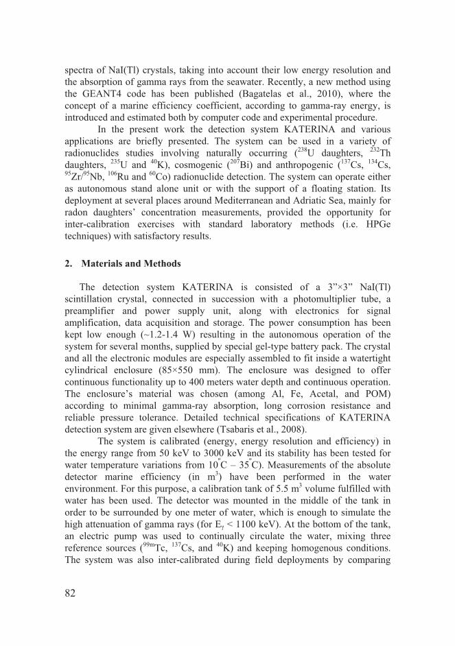
82

spectra of NaI(Tl) crystals, taking into account their low energy resolution and the absorption of gamma rays from the seawater. Recently, a new method using the GEANT4 code has been published (Bagatelas et al., 2010), where the concept of a marine efficiency coefficient, according to gamma-ray energy, is introduced and estimated both by computer code and experimental procedure.

In the present work the detection system KATERINA and various applications are briefly presented. The system can be used in a variety of radionuclides studies involving naturally occurring (238U daughters, 232Th daughters, 235U and 40K), cosmogenic (207Bi) and anthropogenic (137Cs, 134Cs, 95Zr/95Nb, 106Ru and 60Co) radionuclide detection. The system can operate either as autonomous stand alone unit or with the support of a floating station. Its deployment at several places around Mediterranean and Adriatic Sea, mainly for radon daughters’ concentration measurements, provided the opportunity for inter-calibration exercises with standard laboratory methods (i.e. HPGe techniques) with satisfactory results.

2. Materials and Methods

The detection system KATERINA is consisted of a 3”×3” NaI(Tl) scintillation crystal, connected in succession with a photomultiplier tube, a preamplifier and power supply unit, along with electronics for signal amplification, data acquisition and storage. The power consumption has been kept low enough (~1.2-1.4 W) resulting in the autonomous operation of the system for several months, supplied by special gel-type battery pack. The crystal and all the electronic modules are especially assembled to fit inside a watertight cylindrical enclosure (85×550 mm). The enclosure was designed to offer continuous functionality up to 400 meters water depth and continuous operation. The enclosure’s material was chosen (among Al, Fe, Acetal, and POM) according to minimal gamma-ray absorption, long corrosion resistance and reliable pressure tolerance. Detailed technical specifications of KATERINA detection system are given elsewhere (Tsabaris et al., 2008).

The system is calibrated (energy, energy resolution and efficiency) in the energy range from 50 keV to 3000 keV and its stability has been tested for water temperature variations from 10ºC – 35ºC). Measurements of the absolute detector marine efficiency (in m3) have been performed in the water environment. For this purpose, a calibration tank of 5.5 m3 volume fulfilled with water has been used. The detector was mounted in the middle of the tank in order to be surrounded by one meter of water, which is enough to simulate the high attenuation of gamma rays (for E < 1100 keV). At the bottom of the tank, an electric pump was used to continually circulate the water, mixing three reference sources (99mTc, 137Cs, and 40K) and keeping homogenous conditions. The system was also inter-calibrated during field deployments by comparing

83

acquired data of radon’s daughters (214Pb and 214Bi) concentrations with results from water samples measured by HPGe techniques.

Inter-calibration exercises were also performed for the radionuclides 40K, 214Pb, 214Bi and 137Cs. At a location of a submarine groundwater discharge (SGD) at the region of Stoupa, South Peloponnesus, Greece, the results for the concentration of radon daughters obtained from the system were inter-compared with results obtained from a lab-based HPGe technique, measuring samples taken from the same water masses. The samples were collected at the deployment point by divers with Niskin bottles, were stored in a sealed glass bottle and they transported directly to the laboratory. The activity concentration using HPGe technique for 214Pb was estimated (1.1 ± 0.2) Bq/l and for 214Bi (1.2 ± 0.2) Bq/l, while the analysis of KATERINA spectra exhibited similar results (1.0 ± 0.1 Bq/l and 1.3 ± 0.1 Bq/l, respectively).

3. Deployments and Results

3.1. SUBMARINE GROUNDWATER DISCHARGE (SGD)

The system – installed in a special frame along with battery packs – has been deployed for autonomous in-situ operations in various regions in the Mediterranean Sea where submarine groundwater discharges into the coastal zone (Tsabaris et al., 2010). During those deployments, a CTD (Conductivity- Temperature-Density) unit was also used in order to specify the optimum location for the establishment of the detection system according to minimum values of water’s salinity. KATERINA was positioned one meter above the seabed and was obtaining data in real time (on line mode) through a connection with a simple accompanying mobile computer. An indicative spectrum of detected gamma rays acquired during the deployment in Evoikos Gulf, Greece, is shown in Figure 1. Significant concentrations of radionuclides were measured due to the discharging of radon-rich groundwater.

The in-situ system contributes to continuous and autonomous measurements of gamma-ray emitters of interest (daughters of U, Th series) in SGD studies (point sources) with negligible laborious costs. It can also be applied in diffusive sources when the concentration of the radon progenies exceeds the minimum detectable activity (~0.03 Bq l-1). Compared to other radon monitoring systems (e.g. the RAD7), it cannot resolve variations of radon progenies at short-time scales (less than one hour). However, it can be deployed autonomously in deep waters (up to 400 m) for relatively long (up to six months) time periods. Moreover, it is well qualified as a sensor at moorings for the monitoring of artificial radionuclides in seawater (137Cs) or investigations related to submarine earthquakes and radon emanation. When attached to an autonomous underwater vehicle (AUV), it offers the option to map coastal regions for SGD sites on broad spatial scale.

84

Figure 1. A typical gamma-ray spectrum obtained in-situ by KATERINA detector at an SGD location in Evoikos Gulf, Greece.

3.2. MONITORING RADIOACTIVE GASES ON SUBMARINE MAGMATIC REGIONS

Additionally, the system was used in two regions in Adriatic Sea measuring radionuclide in water masses close to magmatic regions (Petrinec et al., 2010). The result of these measurements in depicted in Fig. 2. The significant contribution of 232Th daughters was clearly observed during the measurement performed in Vis Isl., Kroatia. More specifically, 212Pb at 238 keV, which is a 232Th daughter, exhibited an activity concentration of 220 Bq/m3. Also, 208Tl was observed in two energy peaks (583 keV and 2614 keV) and the corresponding measured concentrations were found in good agreement (76 Bq/m3 and 82 Bq/m3, respectively). Furthermore, the concentrations of 222Rn daughters (214Pb and 214Bi) were measured between 115 Bq/m3 and 120 Bq/m3. All natural radionuclide activity concentration was found enhanced compared with those from open sea measurements due to the magmatic origin of the studied region.

85

Figure 2. A typical gamma-ray spectrum obtained in-situ by KATERINA detector at a magmatic orgigin at Adriatic Sea, Kroatia.

3.3. RADIOPROTECTION FOR NORM / TENORM MONITORING

The system is also developed as tool-method for seabed and beach sand mapping in aquatic ecosystems with possible enhanced natural radioactivity. It was deployed at coastal regions where concentrations of Natural Occurring Radionuclide Materials (NORM) and Technologically Enhanced NORM (TENORM) were expected and a baseline study using monitoring methods was requested. At the same time core analysis and measurements of granulometry, geochemistry, mineralogy and organic carbon was implemented. From such studies KATERINA was involved for radionuclide characterization of sediments and beach sand using the grid-based method. By this time a preliminary application in the region of Sounio (Greece) has occurred placing the in-situ detection system 5 cm above the seabed. Additional measurements are in progress as well as analysis of surface and core samples. Further investigation and systematic study is needed in order to have quality assurance exercises by comparing in-situ with lab-based techniques.

3.4. RADON MONITORING NEAR FAULTS

The system was also used for correlating seismicity and radon variation in the groundwater of aquifer in the region of L'Aquila and Teramo, about 120 km from Rome. Advantages of the study area are considered the high seismicity and low-background radiation from cosmic rays. A water tank for the experiment

86

purposes was supplied by groundwater sources discharged inside the mountain. The flow of the water was keeping the tank full during the acquisition time. The overflowing was counterbalanced, providing a water way out through a gate near the basement of the tank. KATERINA was deployed in the middle of the tank. The acquisition period was determined according to an accepted statistical uncertainty of a peak net area calculation. Due to the high radon concentration in the local groundwater, a time lag of 100 min provided accepted statistics (Tsabaris et al., 2011).

A typical spectrum acquired by the system is presented in Figure 3, where peaks of radon daughters, 214Bi (at 609, 768, 1120, 1764 and 2204 keV) and 214Pb (at 351 keV) are clearly observed. The net area calculation for all gamma-ray energies was transformed to activity concentration (Bq/l) using measured and simulated calibration parameters arising from an extensive calibration procedure for the aquatic environment (Bagatelas et al., 2010). The natural radionuclide 208Tl at 583 keV (86%) does not interfere to the analysis of 214Bi at 609 keV, since its concentration is below the limit of detectability as observed in the low-background energy region of the spectrum at 2614 keV (see Fig. 1). The analysis at 609 keV (214Bi) exhibited similar results (within the uncertainty bars) compared with those at 351 keV (214Pb), as expected.

The average concentration of radon daughters was calculated from the aforementioned photopeaks analysis as a mean value of the 214Pb and 214Bi concentrations. The background radon level was arisen approximately 100% during the second acquisition period, although no evidence of an upcoming earthquake via a significant radon activity anomaly was found. The enhanced radon background level in November 2007 compared to the previous measurements (at similar season) is possibly attributed to a gradual increment of microseismicity in the studied region. More specifically, the rate of seismic events greater than 1.3 M has been reported approximately as 310 events/year during 2006 and 2007, while during 2008 it steadily arises up to 570 events/year (Papadopoulos et al., 2010). Similar observations of gradual increment of the radon level were reported previously where radon rose for several years before an earthquake (Asada, 1982). However, a seasonal systematic study including rainfall data could clarify any possible radon level variations due to rainwater-rock interaction inside the aquifer.

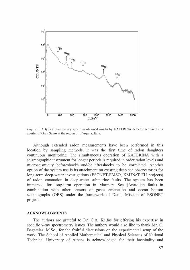
87

Figure 3. A typical gamma ray spectrum obtained in-situ by KATERINA detector acquired in a aquifer of Gran Sasso at the region of L’Aquila, Italy.

Although extended radon measurements have been performed in this

location by sampling methods, it was the first time of radon daughters continuous monitoring. The simultaneous operation of KATERINA with a seismographic instrument for longer periods is required in order radon levels and microseismicity beforeshocks and/or aftershocks to be correlated. Another option of the system use is its attachment on existing deep sea observatories for long-term deep-water investigations (ESONET-EMSO, KM3NeT EU projects) of radon emanation in deep-water submarine faults. The system has been immersed for long-term operation in Marmara Sea (Anatolian fault) in combination with other sensors of gases emanation and ocean bottom seismographs (OBS) under the framework of Demo Mission of ESONET project.

ACKNOWLEGMENTS

The authors are grateful to Dr. C.A. Kalfas for offering his expertise in specific -ray spectrometry issues. The authors would also like to thank Mr. C. Bagatelas, M.Sc., for the fruitful discussions on the experimental setup of the work. The School of Applied Mathematical and Physical Sciences of National Technical University of Athens is acknowledged for their hospitality and

88

scientific support for the experimental work using the calibration tank. Part of this work was supported by the EU project (FP6 contact RII-CT-2004- 506222) through the ERMES project. The authors would like to thank Dr. Gaetano de Luca for his technical support providing the appropriate tank and Prof. Plastino Wolfango for stimulating discussions of the results. The next stage of system applications is already supported under the frame of NoE ESONET project for the deployments in the Marmara Sea.

References

Aakenes, U.R., 1995. Radioactivity monitored from moored oceanographic buoys. Chem. Ecol. 10, 61–69.

Asada, T., 1982. Earthquake Prediction Techniques: Their Application in Japan, University of Tokyo Press.

Bagatelas, C., Tsabaris, C., Kokkoris, M., Papadopoulos, C.T., Vlastou, R., 2010. Determination of marine gamma activity and study of the minimum detectable activity (MDA) in 4pi geometry based on Monte Carlo simulation. Environ. Monit. and Assess. 165, 159–169.

Maucec, M., De Meijer, R.J., Rigollet, C., Hendricks, P.H.G.M., Jones, D.G. 2004. Detection of radioactive particles offshore by g- ray spectrometry part I: Monte Carlo assessment of detection of depth limits. Nucl. Instrum. Methods Phys. Res. A 525, 593–602.

Osvath, I., Povinec, P.P., 2001. Seabed g-ray spectrometry applications at IAEA-MEL. J. Environ. Radioact. 53, 335–349.

Osvath, I., Povinec, P.P., Livingston, H.D., Ryan, T.P., Muslow, S., Commanducci, J.-F., 2005. Monitoring of radioactivity in NW Irish Sea water using a stationary underwater gamma-ray spectrometer with satellite data transmission. J. Radioanal. Nucl. Chem. 263, 437–440.

Papadopoulos, G.A., Charalampakis, M., Fokaefs, A., Minadakis, G., 2010. Nat. Hazards Earth Syst. Sci. 10, 19–24.

Petrinec, B., Franic, Z., Leder, N., Tsabaris, C., Bituh, T., Marovic, G., 2010. Gamma radiation land dose rate investigations on the Adriatic islands of magmatic origin. Rad. Prot. Dosim. 139, 551–559.

Plastino, W., De Felice, P., De Notaristefani, F., 2002. Radon gamma-ray spectrometry with YAP:Ce scintillator. Nucl. Instrum. Methods Phys. Res. A 486, 146–151.

van Put, P., Debauche, A., De Lellis, C., Adam, V., 2004. Performance level of an autonomous system of continuous monitoring of radioactivity in seawater. J. Environ. Radioact. 72, 177–185.

Povinec, P.P., Osvath, I., Baxter, M.S., 1996. Underwater gamma spectrometry with HpGe and NaI(Tl) detectors. Appl. Radiat. Isot. 47, 1127–1133.

Soukissian, T.H., Chronis, G.T., Nittis, K., 1999. POSEIDON: operational marine monitoring system for Greek seas. Sea Technol. 40, 31–36.

Tsabaris, C., Ballas, D., 2005. On line gamma-ray spectrometry at open sea. Appl. Radiat. Isot. 62, 83–89.

Tsabaris, C., Bagatelas, C., Dakladas, Th., Papadopoulos, C.T., Vlastou, R., Chronis, G.T., 2008. An autonomous in situ detection system for radioactivity measurements in the marine environment. Appl. Radiat. Isot. 66, 1419–1426.

Tsabaris, C., Scholten, J., Karageorgis, A.P., Comanducci, J.-F., Georgopoulos, D., Kwong, L., Patiris, D.L., Papathanassiou, E., 2010. Underwater in situ measurements of radionuclides in selected submarine groundwater springs-Mediterranean Sea. Rad. Prot. Dosim. 142, 273–281.

89

Tsabaris, C., Patiris, D.L., Lykousis, V., 2011. KATERINA: An in situ spectrometer for continuous monitoring of radon daughters in aquatic environment. Nucl. Instrum. Methods Phys. Res. A 626-627, S142–S144.

Vlastou, R., Ntziou, I.Th., Kokkoris, M., Papadopoulos, C.T., Tsabaris, C. 2006. Monte Carlo simulation of - ray spectra from natural radionuclides recorded by a NaI detector in the marine environment. Appl. Radiat. Isot. 64, 116–126.

Vlachos, D.S., Tsabaris, C., 2005. Response function calculation of an underwater gamma ray NaI(Tl) spectrometer. Nucl. Instrum. Methods Phys. Res. A 539, 414–420.

Wedekind, C.H., Schilling, G., Gruttmuller, M., Becker, K., 1999. Gamma-radiation monitoring network at sea. Appl. Radiat. Isot. 50, 733–781.

90

TRACK IMAGE ANALYSIS CODE TRIAC II: A TOOL FOR FAST AND

RELIABLE COUNTING OF TRACKS RECORDED BY SSNTD

APPLICATION FOR SPATIAL EXTENSIVE RADON SURVEYS

DIONISIS L. PATIRIS∗, CHRISTOS TSABARIS Hellenic Centre for Marine Research, Institute of Oceanography, P.O. Box 712, GR 19013 Anavyssos, Greece KONSTANTINOS IOANNIDES, KONSTANTINOS STAMOULIS University of Ioannina, Physics Department, Nuclear Physics Laboratory, GR 45110 Ioannina, Greece KONSTANTINOS BLEKAS University of Ioannina, Department of Computer Science, GR 45110 Ioannina, Greece

Abstract. A computer program named TRIAC II written in MatLab has been developed for track recognition and track parameters measurements from images of the Solid State Nuclear Track Detector CR39. The program using image analysis tools counts the number of tracks produced by alpha particles emitted as result of radon and radon daughters decay. At the same time the program may provide geometrical and optical parameters of the tracks for spectrometry purposes of alpha particles. The combined use of SSNT detectors with such fully automated counting techniques may be proved a useful and cost effective tool for spatial extensive radon surveys in the fields of geophysics, in earthquakes precursor studies, and radiation protection of the public.

Keywords: radon, radon anomalies, radon surveys, SSNT detectors, radioprotection.

1. Introduction

The exposure of the general population to ionizing radiation arises primarily from natural sources, which include radionuclides of terrestrial origin and cosmic rays. The dominant contribution, amounting to half of the average received dose, is derived from inhalation of the naturally occurring radon (222Rn) gas and its decay products (UNSCEAR, 2000). Early studies have shown that

∗ Corresponding author Tel.: +302291076408; fax: +302291076323, e-mail address: dpatiris@ath.hcmr.gr

91

the high incidence of lung cancer in miners was associated with exposure to elevated radon concentrations (Uhlig, 1921). Today, radon has been established as the second major cause of lung cancer through epidemiological studies carried out in many countries (BEIR VI, 1999; Darby et al., 2001, 2005; Krewski et al., 2005; Field et al., 2006). Despite radon surveys for radioprotection purposes, the monitoring of radon emanation in the earth’s crust provides information concerning earthquake precursor’s studies. The first observation of radon emanation anomalies prior the occurrence of nearby earthquake was made in the late of 1960s. Till nowadays many studies have been published reporting radon emanation anomalies associated with elevated levels of micro-seismicity and earthquakes. While other gases emanations have also been investigated as possible earthquake precursors, the most of the studies reported in the literature have focused on radon (Cicerone et al., 2009).

Radon is an inert gas so it does not interact chemically with other elements. It defuses easily into the subsoil so it may be transported several meters before decay. Also it may be detected by several methods. Among them, the methods based on Solid State Nuclear Track Detectors (SSNTD) provide a cost effective and reliable tool for radon mapping over spatial extensive regions. There are several different types of such detectors (CR-39, LR-115, CA 80-15 etc) having all the same principle of detection. Following the passage of a charged particle through a SSNTD a damage region is created usually named latent track. Latent tracks can be etched using a suitable etchant (i.e. NaOH or KOH), sufficiently enlarging them to become visible under an optical microscope (with diameters of 1 m or more). Using the appropriate apparatus one can take images of the SSNTDs surface and count the number of the tracks which is proportional to the activity concentration of radon. However, the manual counting is a tedious and time-consuming task, so an automatic system is needed to speed up the process. A number of automatic track counting systems have been reported (Molnar et al., 1984; Dreute et al., 1986; Fews 1992; Bookhair et al., 2000; Patiris et al., 2006; Patiris et al., 2007), which recognize tracks on the basis of the grey level of images. The code presented here, is based on a segmentation method that groups image pixels in a number of grey level groups chosen by the user. After the segmentation of pixels, TRIAC counts the tracks that were recorded, even those tracks which overlap each other and estimates their geometrical (major and minor axes in case of elliptical tracks) and optical (mean value of brightness) parameters for alpha-particle spectroscopy purposes.

2. TRIAC II Code

2.1. GENERAL INFORMATION

The program TRIAC II is written in the high level language MatLab which is accompanied by a variety of tools for special applications. To use the program

92

the user should install a version of MatLab (7.0 or newer) along with the Statistical toolbox and the Image Processing Toolbox. TRIAC II could be downloaded free for scientific purposes from the program library of Computer Physics Communication journal. It runs in two different modes followed by the corresponding calibration actions. The first mode is dedicated to the estimation of the number of the tracks from a SSNTD’s surface image. The accurate measurement of the number of tracks is important for reliable radiation dose estimations. Usually, a number of images are required, containing as many tracks as possible for improved statistics. To include a large number of tracks in an image, lenses of low magnification may be used. As a result, most tracks are resolved as circles. For this reason the program counts the tracks as circles, when is functioning in the first mode. On the other hand, in the second mode the user is provided with the parameters of the recognized tracks, which in general have elliptical shapes. The major and minor axes (in pixels), the mean value of brightness and the orientation (in degrees) of the tracks are output in files. The results are more accurate if a lens of higher magnification is used. Also, in the calibration modes, a group of images is provided on screen. This group contains the initial and a number of analyzed images produced after certain program steps. The aim of the calibration modes is to help the user set the input program parameters, which fit better to his/her criteria. Finally, TRIAC II is supplied with a GUI, which facilitates the entry of input parameters and the choice of actions. A general flow diagram of the program is presented in Fig. 1.

2.2. IMAGE SEGMENTATION

An image of a SSNTD’s surface is represented in MatLab as a two-dimensional matrix of size equal to the image’s digital resolution. TRIAC II is applied to greyscale images, in which grey scale intensities are represented using 8-bits per pixel (jpeg images). The first step of the analysis is the image segmentation task that groups the image pixels together and separates the objects (the useful information) from the background. A variety of methods have been proposed for image segmentation, such as the edge- based or the region-based methods (Pal and Pal, 1993). Amongst them, histogram-based clustering methods have been proved very efficient, since they correspond to

93

Figure 1 The flow diagram of the TRIAC II program. clustering approaches. A well-known clustering method is the K-means algorithm (Duda et al., 2001), which tries to appropriately adjust the K cluster centres in order to minimize the distance from each data point to its nearest centre. In the case of TRIAC II program the data points are the pixel intensity values. The algorithm estimates K centres (pixel intensity values) and groups all pixels accordingly. The criterion for a value to be a cluster’s centre is the minimization of the sum of the distances from the nearest cluster centre. However, the term “distance” used here is not a real-space distance but actually it is the absolute difference of intensities.

94

Due to its local search, a known drawback of the algorithm is the initialization of their parameters (centres). This is accomplished by uniformly selecting a small subset of the pixel intensities (e.g., 10%) and executing the algorithm several times. The optimum solution found is then used for initializing the cluster centres. The number of these cluster centres K is entered by the user. As it has been observed, the input images, apart from the background (light pixels) and the track regions (dark pixels), contain a middle level(s) of brightness pixel regions (grey). This happens due to system imperfections during the generation process. Therefore, a value of K = 3 or 4 is used for the number of clusters during the clustering procedure to optimally distinguish the useful information (track objects) from the remaining parts of the image. At the end of the segmentation process, every pixel is labeled with a discrete value in the range of [1, K] based on the cluster it belongs (minimum distance from the cluster centres). Since we are interested in the track objects, a binary image is finally produced by setting only the darker pixels to the value one (1) and leaving the rest as zero (0). An example of the whole segmentation process is presented in Fig. 2.

It must be noted that before the image segmentation and in the second mode of TRIAC II, a brightness normalization procedure of the initial image is performed. This step aims to reduce the influence of apparatus characteristics or imperfections in the measurement of pixel intensities. In some cases the background in photos containing particle tracks is not uniform. In addition because of apparatus imperfections the detector’s photo may contain objects, which are not real tracks. The center of the image is brighter and if a track was located there, its mean brightness value would be overestimated. Also, there are some “track-like” objects, which are not objects from the detector’s surface but results of apparatus imperfections and obviously are not real tracks. These phenomena can increase the number of observed tracks and may affect the accuracy of brightness measurements.

The Brightness normalization step obliterates such problems. A user in addition to the detector’s photos has to provide a back- ground photo. For this photo, a user has not to include the detector itself but he must be careful to keep exactly the same apparatus adjustments (i.e. magnification, focusing) with which the tracks’ photos were recorded. The grey scale pixel values of this photo, which must be named “BrightNormal.jpg”, include any brightness in homogeneities or imperfections of the apparatus and are subtracted from corresponding values of the detector photos.

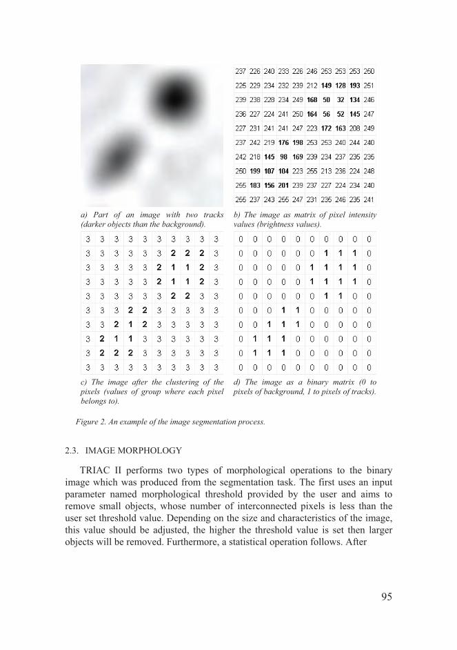
95

a) Part of an image with two tracks (darker objects than the background).

b) The image as matrix of pixel intensity values (brightness values).

c) The image after the clustering of the pixels (values of group where each pixel belongs to).

d) The image as a binary matrix (0 to pixels of background, 1 to pixels of tracks).

Figure 2. An example of the image segmentation process.

2.3. IMAGE MORPHOLOGY

TRIAC II performs two types of morphological operations to the binary image which was produced from the segmentation task. The first uses an input parameter named morphological threshold provided by the user and aims to remove small objects, whose number of interconnected pixels is less than the user set threshold value. Depending on the size and characteristics of the image, this value should be adjusted, the higher the threshold value is set then larger objects will be removed. Furthermore, a statistical operation follows. After

96

a) Initial image b) The image after brightness normalization

c) The image before the morphology step. d) The image after the morphology step.

Figure 3. An example of brightness normalization step and morphology operations. removing small objects, the program performs an initial estimation of all objects sizes and their average size together with the associated standard deviation. Then, objects with sizes greater than the mean value plus n-times the standard deviation are removed. An input value named statistical check value is related to the procedure described above that aims to remove imperfections on the detectors’ surfaces or other oversized objects, which are not tracks. Setting this value low will allow more objects to be removed since their size exceeds the average size. The morphological threshold value and the statistical check value are determined using the calibration modes. In Fig.3 an example of the brightness normalization step and the morphology operations is presented.

2.4. TRACKS DETECTION

The next step in the analysis is the determination of the number, as well as the geometric features of the tracks in the isolated objects of the resulting binary image. These objects may contain one or more overlapping tracks. In order to separate them, we followed the next strategy: In each object, we initially perform the Canny edge detection algorithm (Canny, 1986) to find object boundaries in the image. The known Hough transform (Parker, 1997; Yip et al., 1992) approach is then applied to identify the geometric structure of the tracks. In the first mode, as it was already mentioned, the tracks are considered circular

97

so we apply the circular Hough transform. In this way, we extract the length of the diameter (in pixels) and the mean intensity value of each detected circular track. In the second mode a more complicated procedure is followed dealing with the general case of the elliptic shape of tracks. Here, we apply the Hough transform approach for ellipses (Yip et al., 1992) and the output includes four features: the major axis, the minor axis, the orientation of the ellipse, and the mean intensity value of the surrounding pixels. In either case, we build an appropriate Hough space of dimensions equal to the parameters of the assumed geometric shape, where the Hough transform tries to fit any observed object with a number of objects of the appropriate shape (circle or ellipse) and its strongest peaks correspond to the number of the overlapping tracks in the object. The method iteratively detects the strongest peak and then sets the values of the accumulator function in the surrounding pixels to zero in order to avoid re-detecting the same feature during the next steps. This process continues until the number of remaining pixels in the current object is smaller than an internal and predefined threshold value. An example is presented in Fig. 4 in the case of the circular Hough transform.

Figure 4. The recognition of overlapped tracks using Hough transform for circular tracks.

2.5. GRAPHICAL USER INTERFACE

In order to use the TRIAC II code, a MatLab v7.0 (or a newer version), the statistical toolbox and the image processing toolbox must be available. Before running the code a user has to create a working folder in which all the images are placed. Also this folder should include the special image file named BrightNormal.jpg, which represents the brightness distribution of the images’ background, all the 12 TRIAC II’s .m files (containing the TRIAC II code) and a text file where the names of images must be listed as imagename.jpg. If it is desired the images can be grouped by naming them using the same n-characters (letters or numbers) as the first characters in their filenames. This number of the

98

same characters is another input value, which the user has to set on the GUI. After initializing MatLab, the user has access to the specified working folder using the MatLab’s task bar.

When this step is completed in the command window, the user has to type TRIAC_II or double click the TRIAC_II.fig icon in the current directory window and the TRIAC II GUI will appear. In this state the user has to enter data to the program, completing the edit boxes with the name of .txt file, where the names of images are written, the length of the string which will name a group of images, the values for the number of clusters, the morphological threshold value, the morphological statistical check value and to specify if he/she wishes to produce histograms for any separate image or (and) for any image group. After completing the GUI’s edit boxes, the user has only to click on the action button to initialize the desired mode of TRIAC II.

The most important parameters, which must be provided, are the number of clusters and the two morphological operator parameters. These will determine the final binary image which the Canny edge detection algorithm and the Hough functions will process. For an accurate measurement these parameters must be chosen carefully. It is strongly recommended to the user before any extensive counting to select a small number of representative images, and using the test modes of the program to determine the values that best fit certain criteria. A usual way is to keep one value constant (e.g., the number of clusters), then to adjust the other parameters running the test modes and from the resulting images to select the most appropriate combinations.

3. Conclusion

The program TRIAC II written in MatLab is useful for experimental measurements involving nuclear track detectors. It enables measurements of tracks’ number and parameters like the axis (diameter) of an elliptical (circle) track, the mean value of their brightness and the orientation. The program is user friendly and demands a MatLab 7 or newer installation plus the Statistical and Image Processing toolboxes. When used in a systematic way, it provides reliable counting results of a big number of images even when overlapping tracks do exist.

ACKNOWLEGMENTS

This work was partly funded by the Greek Secretariat of Research and Technology (Contract GSRT-174 )

99

References

Beir VI: Committee on Health Risks of Exposure to Radon Health Effects of Exposure to Radon, 1999. National Academy Press, Washington, DC, ISBN 0-309- 05645-4.

Boukhair, A., Haessler, A., Adloff, J.C., Nourreddine, A., 2000. New code for digital imaging system for track measurements Nucl. Instr. and Meth. B 160, 550-555.

Canny, J., 1986. IEEE Transactions on Pattern Analysis and Machine Intelligence 8, 679. Cicerone, R.D., Ebel, J.E., Britton, J., 2009. A systematic compilation of earthquake precursors,

Tectonophys. 476, 371-396. Darby, S., Hill, D., Doll, R. ,2001. Radon: a likely carcinogen at all exposures. Ann. Oncol. 12,

1341-1351. Darby,S.,Hill,D.,Auvinen,A.,Barros-Dios,J.M.,Baysson,H.,Bochicchio,F.,etal., 2005. Radon in

homes and risk of lung cancer: collaborative analysis of individual data from 13 European case-control studies. Br .Med. J. 330, 223-227.

Dreute, J., Trakowski, W., Schofer, B., Brectman, C., Drechel, H., Eversberg, H., Fricke, W. , Beer, J., Wiegel, B., Heinrich, W., 1986. The Siegen automatic measuring system for nuclear track detectors status and new developments Nucl. Tracks Rad. Meas. 12, 261-264.

Duda, R.O. , Hart, P.E., Stork, D.G., 2001. Pattern Classification, Wiley-Interscience, New York Fews, A., 1992. Flexible analysis of etched nuclear particle tracks, Nucl. Instr. and Meth. B 72,

91-103. Field, R.W., Krewski, D., Lubin, J.H., Zielinski, J.M., Alavanja, M., Catalan, V.S., Klotz, J. B.,

Létourneau, E.G., Lynch, C.F., Lyon, J.L., Sandler, D.P., Schoenberg, J.B., Steck, D. J., Stolwijk, J.A., Weinberg, C., Wilcox, H.B., 2006.An overview of the North American residential radon and lung cancer case-control studies. J. Toxicol Environ. Health A69, 599-631.

Krewski, D., Lubin, J.H., Zielinski, J.M., Alavanja, M., Catalan, V.S., Field, R.W., Klotz, J. B., Létourneau, E.G., Lynch, C.F., Lyon, J.I., Sandler, D.P., Schoenberg, J.B., Steck, D. J., Stolwijk, J.A., Weinberg,C., Wilcox, H.B., 2005. Residential radon and risk of lung cancer: a combined analysis of 7 North American case-control studies. Epidemiology 16,137-145.

Molnar, J., Somogyi, S., Szilagyi, S., Spesi, K. 1984. Development of a CCD based system called digitrack for automatic track counting and evaluation Nucl. Tracks Rad. Meas. 8 243-246.

Pal, N.K., Pal, S.K., 1993. A review of image segmentation techniques, Pattern Recognit. 26, 1277-1294.

Parker, J.R., 1997. Algorithms for Image Processing and Computer Vision, John Wiley & Sons, Inc., New York.

Patiris, D.L., Blekas, K., Ioannides, K., 2006. TRIAC: A code for track measurements using image analysis tools, Nucl. Instr. and Meth. B 244, 392-396.

Patiris, D.L., Blekas, K., Ioannides, K., 2007. TRIAC II A MatLab code for track measurements from SSNT detectors, Comp. Phys. Comm. 177, 329-338.

UNSCEAR (United Nations Scientific Committee on the Effects of Atomic Radiation) 2000. Sources and Effects of Ionizing Radiation. Report to General Assembly, with Scientific Annexes. United Nations New York.

Uhlig, M.,1921.Uber den Schneeberger Lungenkrebs.Virchows Arch. Pathol. Anat. Physiol. Klin. Med. 230, 76-98.

Yip, R.K.K., Tam, P.K.S., Leung, D.N.K., 1992. Modification of Hough transform for circles and ellipses detection using a 2-dimensional array, Pattern Recognition 25 1007–1022.

100

METHODS FOR LONG-TERM RADON TIME-SERIES EVALUATION

GREGORI A., ZMAZEK B., VAUPOTI J. Department of Environmental Sciences, Jožef Stefan Institute, Jamova 39, 1000 Ljubljana, Slovenia

Abstract: Noble gas radon (222Rn) originates from radioactive transformation of 226Ra in the 238U decay chain in the Earth’s crust. The measurement of spatio-temporal variation of radon in soil or water has given evidence that the emanation of this gas can be related to tectonic stress-strain variations in the crust. The influence of meteorological parameters, controlling radon exhalation from the Earth’s crust, makes it complicated and for small earthquakes often impossible to differentiate the anomalies caused by seismic events from those caused solely by atmospheric changes. Different approaches can be used for this purpose. In the first approach radon anomalies are defined as deviations in radon concentration of more than ± (multiple x of standard deviation ) from the average seasonal value. The second approach takes into account the inverse relationship between radon exhalation and barometric pressure. Finally, machine learning methods can be effectively applied as a tool for identification of radon anomalies.

Keywords: radon, earthquake precursor, radon anomaly, decision trees, artificial neural networks

1. Introduction

Radon is one of many geophysical and geochemical phenomena that can be considered to be an earthquake precursor. The term “earthquake precursor” is used to describe a wide variety of geophysical and geochemical phenomena that reportedly precede at least some earthquakes [1]. The observation of these types of phenomena is one of the recent research activity which has aimed at reducing the effects of natural hazards. Among the different precursors, geochemistry has provided some high-quality signals, since fluid flows in the Earth’s crust have a widely recognized role in faulting processes [2]. The potential of gas geochemistry in seismo-tectonics has been widely discussed by Toutain and Baubron [3].

In the late 1960s and early 1970s, reports from seismically active countries such as the former USSR, China, Japan and the USA [4–6], indicated that concentrations of radon gas in the earth apparently changed prior to the occurrences of nearby earthquakes [7]. The noble gas radon originates from

101

radioactive transformation of 226Ra in the 238U decay chain in the Earth’s crust. Since radon is a radioactive gas, it is easy and relatively inexpensive to monitor instrumentally, and its short half-life (3.82 days) means that short-term changes in radon concentration in the earth can be monitored with very good time resolution. Radon emanation from grains depends mainly on 226Ra content and mineral grain size, its transport in the earth governed by geophysical and geochemical parameters [8], while exhalation is controlled by hydrometeorological conditions. The stress-strain developed within the Earth’s crust before an earthquake leads to changes in gas transport and a rise of volatiles from the deep earth up to the surface [9, 10], resulting in anomalous changes in radon concentration. The mechanism of observed radon anomalies is still poorly understood, although several theories were proposed [11–13]. Over the past three decades the occurrence of anomalous temporal changes of radon concentrations has been studied by several authors specialising in soil gas [6, 14–20] and groundwater [21–27]. However, radon anomalies are not only controlled by seismic activity, but also by meteorological parameters like soil moisture, rainfall, temperature and barometric pressure [10, 28]. This makes it complicated and, for small earthquakes, often impossible to differentiate between the anomalies caused by seismic events from those caused solely by atmospheric changes. Therefore, the application of theoretical and empirical algorithms for removing meteorological effects is necessary [29–32]. In this paper, the different approaches to distinguishing between those anomalies in radon time series caused by seismic activity and those caused solely by hydrometeorological parameters are presented and discussed.

2. Radon migration in the Earth’s crust

Only a fraction of the radon atoms created by radioactive transformation from radium are able to emanate from mineral grains and enter into the void space, filled either by gas or water. Radon ascends towards the surface mainly through cracks or faults, on a short scale by diffusion and, for longer distances, by advection - dissolved in either water or in carrier gases. Gas movement should be ascribed to the combination of both processes. Diffusive movement is driven by a concentration gradient and is described by Fick’s law. Due to low velocity of radon transport, diffusion is important only in capillaries or small-pored rocks [8, 33]. On the other hand, the velocity and space scales of advective movements are much higher than those of diffusive ones. Advective transport is driven by pressure gradients, following Darcy’s law. The amount of radon itself is, however, too small to form a macroscopic quantity of gas which can react to pressure gradients. Therefore, it must be carried by a macroscopic flow of carrier gases [34]. A gas mixture formed by carrier gases (e.g. CO2, CH4, N2) and rare gases (e.g. He, Rn) can be referred to as “geogas” [8, 34].

102

2.1. EXTERNAL EFFECTS ON RADON IN SOIL GAS AND WATER

Radon concentration in soil gas or water is not only controlled by geophysical parameters, it also changes due to meteorological effects, which change physical characteristics of soil and rock, thus influencing the rate of radon transport and, consequently, perturbing eventual radon variations caused by geophysical processes originating in deeper parts of the Earth’s crust. Shallow soil levels are more affected by changing meteorological conditions than deeper ones. Radon concentrations with no larger variations present are usually observed at depths of 0.8 m or deeper. Besides the effects of meteorological parameters on radon in soil gas, considerable variations of gas composition of thermal springs have been shown to be the result of fluctuations of local hydrologic regimes [35].

The significant influence of barometric pressure has been discussed by several authors, who clearly pointed out an inverse relationship between barometric pressure and radon concentration in soil gas [35, 36]. Numerous and often divergent results in studies related to the effect of external factors on soil gas radon concentration suggest that no general predictive model for excluding meteorological effects can be proposed, and studies of radon in soil gas need simultaneous record of meteorological parameters.

2.2. ANOMALOUS RADON CONCENTRATION AND SEISMICITY

Both mechanisms of radon transport – diffusion and advection – depend on both soil porosity and permeability, which at the same time vary as a function of the stress field [37]. However, migration by diffusion is negligible, where a component of advective long-distance transport exists [8]. The high permeability of the bedrock and soil in areas of crustal discontinuities, such as fractures and fault zones, promotes intense degassing fluxes, which causes higher soil gas radon concentrations on the ground surface above active fault zones. Although several measurements, experiments and models have been performed, the understanding of the mechanism of radon anomalies and their connection to earthquakes is still inadequate [38, 39]. Several mechanisms have been proposed, which could explain the relationship between radon anomaly and earthquake. According to a compression mechanism for radon release, proposed by King [11], the anomalous high radon release may be due to an increase of crustal compression before an impending earthquake that squeezes out soil gas into the atmosphere at an increasing rate.

Toutain and Baubron [3] observed that gas transfer within the upper crust is affected by strains less than 10–7, much smaller than those causing earthquakes.

103

According to Dobrovolsky [40] the radius of the effective precursory manifestation zone depends on the earthquake magnitude and can be calculated using the empirical equation:

(1)

Where RD is strain radius in km and ML is the magnitude of the earthquake.

2.3. METHODS FOR DETECTING ANOMALIES IN RADON TIME SERIES

An anomaly in radon concentration is defined as a significant deviation from the mean value. Due to the high background noise of radon time series it is often impossible to distinguish an anomaly caused solely by a seismic event, from one resulting from meteorological or hydrological parameters. For this reason, the implementation of more advanced statistical methods in data evaluation is important [41–43]. In our research, radon has been monitored in several thermal springs [21, 23, 24] and in soil gas [19] and different approaches of distinguishing radon anomalies were applied.

2.4. STANDARD DEVIATION

A very common practice in determining radon anomalies is the use of standard deviation. The average radon concentration is calculated for different periods with regard to the nature of yearly cycles of radon concentration. In the case of radon in soil gas, the mean value of radon concentration is calculated separately for four seasons (spring, summer, autumn and winter) based on the air and soil temperature.

In contrast to soil gas, radon in ground or spring water is greatly influenced by the hydrologic cycle, which has to be considered during the data analysis. To define the mean and standard deviation, anomalously high and low values – which may cause unnecessary high deviation and perturb the real anomalies – have to be neglected. The periods when radon concentration deviates by more than ±2 from the related seasonal value are considered as radon anomalies that are possibly caused by earthquake events and not by meteorological parameters [19, 21, 44, 45].

2.5. RELATIONSHIP BETWEEN RADON EXHALATION AND BAROMETRIC PRESSURE

An inverse relationship exists between the time derivative of radon concentration in soil gas and time derivative of barometric pressure. A decrease

104

in barometric pressure causes an increase in radon exhalation from the ground, whereas during periods of rising pressure, air with low radon concentration is forced into the ground, thus diluting radon concentration. Therefore deviations from this rule during these periods – when the time gradient of barometric pressure, P/ t, and the time gradient of radon concentration, CRn/ t, in soil gas have the same sign – can be considered to be radon anomalies [19].

2.6. MACHINE LEARNING METHODS

Machine learning methods have been successfully applied to many problems in the environmental sciences. In the case of radon as an earthquake precursor, it must be considered – as discussed in section 2.1 – that the variation in radon concentration is controlled not only by geophysical phenomena in the Earth’s crust, but also by the environmental parameters associated with the radon monitoring sites. With machine learning methods, a model for the prediction of radon concentration can be built, taking into account environmental parameters(e.g. barometric pressure, rainfall and air and soil temperature). The aim is to identify radon anomalies which might be caused by seismic events.

2.6.1. Artificial neural networks

An artificial neural network (ANN) is a well known computational structure inspired by the operation of the biological neural system [46] and is well established tool, being used widely in signal processing, pattern recognition and other applications. An ANN consists of a set of units (neurons, nodes), and a set of weighted interconnections among them (links). The organization of neurons and their interconnections defines the net topology. The inputs are grouped in an input layer, outputs in an output layer and all the other units in so called hidden layers. The algorithm repeatedly adjusts the weights to minimise the mean square error between the actual output vector and the desired network output vector. The universal approximator functional form of ANNs is well-suited for the requirements of modelling non-linear dependency of radon concentration on multiple variables. Among a number of various topologies, training algorithms and architectures of ANNs, the traditional multilayer perceptron (MLP) with a conjugate gradient learning algorithm was chosen in the case of analysing soil gas radon concentration time series at the Krško basin [31]. The series was first split into seismically non-active periods (NSA) and seismically active periods (SA), adjusting the duration of the seismic window from 0 to 10 days before and after the earthquake and with the purpose of investigating the influence of a complete earthquake event on radon concentration (the preparation phase, the earthquake itself and aftershocks). The ANN of the MLP type was trained with each of NSA datasets, which were divided into three sets: the training set (60%),

105

the cross-validation set (15%) and the test set (25%). The ANN was trained with the training and cross-validation set, while the test set was used to verify its performance. In the testing phase, the correlation between the measured (m-CRn) and predicted (p-CRn) radon concentration in NSA periods was compared to the correlation between the measured and predicted radon concentration in the entire dataset (NSA and SA). The difference between the correlation coefficients might indicate a period of seismically induced radon anomaly. The ratio between measured and predicted values (m-CRn/p-CRn)–1 represents the discrepancy between both values. A radon anomaly is held to be when the absolute value of signal (m-CRn/p-CRn)–1 exceeds the predefined threshold of 0.2.

2.6.2. Decision trees

Decision trees are machine-learning methods for constructing prediction models from data. The models are obtained by recursively partitioning the data space and fitting a simple prediction model within each partition. As a result, the partitioning can be represented graphically as a decision tree, where each internal node contains a test on an attribute, each branch corresponds to an outcome of the test, and each leaf node gives a prediction for the value of the class variable [47, 48]. Regression trees are designed for dependent variables that take continuous or ordered discrete values. Like classical regression equations, they predict the value of a dependent variable (called class) from the values of a set of independent variables (called attributes).

The model in each leaf can be a linear equation or just a constant. Trees having linear equations in the leaves are also called model trees. Tree construction proceeds recursively, starting with the entire set of training examples. An important mechanism used to prevent the tree from over-fitting data is tree pruning. Regression (RT) and model trees (MT), as implemented with the WEKA data mining suite [49], were used for predicting radon concentration from meteorological parameters in the case of radon time series in soil gas at Krško basin [18, 32] and in thermal spring water in Zatolmin [24].

The first stage of data analysis comprises the selection of attributes, i.e. environmental parameters, and partitioning of the whole data set to the periods with and without seismic activity, SA and NSA respectively. After inspecting correlation changes between radon concentration and barometric pressure, a seismic window of ±7 days was chosen. The performance was estimated with 10-fold cross validation in order to evaluate the predictability of radon concentration in the NSA periods. The model built on NSA data set was then applied to the SA data set and the performance change was determined using two different measures, correlation coefficient (r) and root mean square error (RMSE). For the prediction purpose, the measured performance in NSA periods should be higher than the performance in SA periods. In the periods, when the discrepancy between measured and predicted radon concentration is low, no

106

seismic activity is anticipated, while in the periods with higher discrepancy, a radon anomaly can be ascribed to increased seismic activity, rather than to the effect of atmospheric parameters. A radon anomaly is held to be when the absolute value of signal (m-CRn/p-CRn)–1 exceeds the predefined threshold of 0.2. Besides regression trees also other machine learning methods were tested (e.g. linear regression and instance based regression). However, model trees have been shown to outperform other approaches.

2.7. COMPARISON OF THE RESULTS

The results of all of the approaches used for identification of radon anomalies caused by seismic events in the case of soil gas radon at Krško basin are shown in Fig. 1 for the period of 1/9 – 30/12/2000.

Among all of the approaches –and although not very exact – the ±x method (I) is the most frequently used. The threshold of anomalous concentrations (e.g. ±1 , ±2 , ±3 ) should be chosen in order to minimize the number of false anomalies (FA: anomalies in seismically non-active periods) and so as not to miss the correct ones (CA). Generally, a range of ±2 from the related seasonal mean value is chosen. Furthermore, a cyclic behaviour of radon concentration has to be taken into account in order to accurately define the period of standard deviation and the calculation of the mean value. For this purpose different methods of time series analyses – for example Fourier transform [22] – can be applied.

In the case shown in Fig. 1a, three radon anomalies exceeding 2 above mean value may be noticed. The first, in the beginning of September, cannot be assigned to a seismic event (FA). About a week before a weak earthquake of local magnitude ML=1.1, 5 km away from the measurement location – which is the first of five earthquakes over a period of 2 months – the second anomaly is observed. And finally, the third one can be noticed soon after a weak earthquake 6 km away (ML=1).

The first anomaly mentioned above as FA is visible also by applying the method of pressure gradients (II) (Fig. 1b). A positive correlation between the time gradient of radon concentration and the time gradient of barometric pressure is considered to be radon anomaly, and corresponds to the anomaly observed through method (I), which preceded the first earthquake (ML=1.1). A radon anomaly can also be noticed a few days before the last earthquake, as with the analysis of method (I). Additionally, the anomalous behaviour of radon concentration as regards the gradient approach is observed during the period starting a few days before the earthquake with ML=2.7 and lasting untill the earthquake with ML=1. More often than not swarms of anomalies are observed over longer periods, with higher number of anomalies in a swarm observed for

107

the approach (II) than for the approach (I). As an additional criterion, a threshold of P/ t > 2 hPa d–1, is introduced in this approach in order to optimize the identification of anomalies caused by seismic events. However, by increasing the threshold value above 2 hPa d–1, the ratio between correct and false anomalies cannot be significantly improved [18].

Both machine learning approaches, artificial neural networks (III) and decision trees (IV) give promising results, with a low number of false anomalies. The two distinctive anomalies – observed in Fig. 1c and Fig. 1d, for ANN and MT, respectively – confirm the anomalies identified by approaches (I) and (II). Additionally, a relatively long negative anomaly was observed using the ANN approach at the end of November, accompanying the earthquake with ML=1.6. On the other hand, the same negative anomaly is only weakly expressed using the MT approach. A FA observed at the

Fig. 1: Comparison of different approaches for identification of radon anomalies: a) standard deviation (I), b) relationship between radon exhalation and barometric pressure (II), c) artificial neural networks (III) and d) model trees (IV).

108

Beginning of September using approaches (I) and (II) was also noticed using the MT approach but not by the ANN approach. The approaches (III) and (IV) do not appear to greatly depend upon the choice for the threshold of (m-CRn/p-CRn)–1 and can, therefore, be used by less hesitation.

3. Conclusion

Since the appropriate interpretation of field measurements plays an important role in any research, the purpose of this work was to combine and evaluate the different approaches applied by our research group for differentiating the radon anomalies caused by increased seismic activity from those caused solely by environmental parameters. The application of four different approaches – standard deviation from the related men value (I), the correlation between time gradients of barometric pressure and radon concentration (II), artificial neural networks (III) and decision trees (IV), was presented. Radon anomalies based on approach (I) have been less successful in predicting earthquakes than those based on the other three approaches. Secondly, approaches (I) and (II) greatly depend upon the values of the ±x and P/ t thresholds, respectively, while the dependence of approaches (III) and (IV) on the threshold of (m-CRn/p-CRn)–1 is very weak. The number of false anomalies at the approach (II) points out to the disturbance of radon exhalation by other environmental parameters and not just by barometric pressure. The assumption that radon exhalation is only directly influenced only by barometric pressure is further suggested by different forms of radon transport at compression and dilatation zones [10]. Promising results are achieved by applying approaches (III) and (IV), which make it possible to simultaneously incorporate all of the available environmental parameters. Furthermore, in using these techniques, the relation between radon concentration and environmental parameters does not necessarily have to be presumed linear. And finally, in taking into account the scale of the earthquake magnitudes observed during the time of radon measurements, one may speculate that the performance of the applied approaches would be better in the case of stronger earthquakes.

References:

1. Cicerone, R.D., J.E. Ebel, and J. Britton, A systematic compilation of earthquake precursors. Tectonophysics, 2009. 476(3–4): p. 371–396.

2. Hickman, S., R. Sibson, and R. Bruhn, Introduction to special section: Mechanical involvement of fluids in faulting. Journal of Geophysical Research, 1995. 100(B7): p. 12831–12840.

3. Toutain, J.P. and J.C. Baubron, Gas geochemistry and seismotectonics: a review. Tectonophysics, 1999. 304(1–2): p. 1–27.

109

4. Ulomov, V.I. and B.Z. Mavashev, On forerunners of strong tectonic earthquakes. Doklady Akademii Nauk SSSR, 1967(176): p. 319–322.

5. Wakita, H., et al., Radon anomaly - possible precursor of the 1978 Izu-Oshima-Kinkai earthquake. Science, 1980. 207(4433): p. 882–883.

6. King, C.Y., Anomalous radon emanation of San Andreas fault. Transactions-American Geophysical Union, 1976. 57(12): p. 957–957.

7. Lomnitz, C., Fundamentals of Earthquake Prediction1994, New York: John Wiley & Sons. 8. Etiope, G. and G. Martinelli, Migration of carrier and trace gases in the geosphere: an

overview. Physics of the Earth and Planetary Interiors, 2002. 129(3–4): p. 185–204. 9. Thomas, D., Geochemical precursors to seismic activity. Pure and Applied Geophysics, 1988.

126(2): p. 241–266. 10. Ghosh, D., A. Deb, and R. Sengupta, Anomalous radon emission as precursor of earthquake.

Journal of Applied Geophysics, 2009. 69(2): p. 67–81. 11. King, C.Y., Radon emanation on San Andreas Fault. Nature, 1978. 271(5645): p. 516–519. 12. Martinelli, G. Fluidodynamical and chemical features of radon 222 related to total gases:

implications for earthquake predictions. in IAEA Meeting on isotopic and geochemical precursors of earthquakes and volcanic eruptions. 1991. Vienna, September 1991.

13. Atkinson, B.K., Stress corrosion and the rate-dependent tensile failure of a fine-grained quartz rock. Tectonophysics, 1980. 65(3–4): p. 281–290.

14. Planini , J., V. Radoli , and Ž. Lazanin, Temporal variations of radon in soil related to earthquakes. Applied Radiation and Isotopes, 2001. 55(2): p. 267–272.

15. Walia, V., et al., Continuous temporal soil-gas composition variations for earthquake precursory studies along Hsincheng and Hsinhua faults in Taiwan. Radiation Measurements, 2009. 44(9–10): p. 934–939.

16. Reddy, D.V. and P. Nagabhushanam, Groundwater electrical conductivity and soil radon gas monitoring for earthquake precursory studies in Koyna, India. Applied Geochemistry, 2011. 26(5): p. 731–737.

17. Mogro-Campero, A., R.L. Fleischer, and R.S. Likes, Changes in subsurface radon concentration associated with earthquakes. Journal of Geophysical Research, 1980. 85(NB6): p. 3053–3057.

18. Zmazek, B., et al., Radon in soil gas: How to identify anomalies caused by earthquakes. Applied Geochemistry, 2005. 20(6): p. 1106–1119.

19. Zmazek, B., et al., Soil radon monitoring in the Krško Basin, Slovenia. Applied Radiation and Isotopes, 2002. 56(4): p. 649–657.

20. Kuo, T., et al., Application of recurrent radon precursors for forecasting large earthquakes (Mw > 6.0) near Antung, Taiwan. Radiation Measurements, 2010. 45(9): p. 1049–1054.

21. Gregori , A., B. Zmazek, and J. Vaupoti , Radon Concentration in Thermal Water as an Indicator of Seismic Activity. Collegium Antropologicum, 2008. 32: p. 95–98.

22. Ramola, R.C., Relation between spring water radon anomalies and seismic activity in Garhwal Himalaya. Acta Geophysica, 2010. 58(5): p. 814–827.

23. Zmazek, B., et al., Geochemical monitoring of thermal waters in Slovenia: relationships to seismic activity. Applied Radiation and Isotopes, 2002. 57(6): p. 919–930.

24. Zmazek, B., et al., Radon in a thermal spring: Identification of anomalies related to seismic activity. Applied Radiation and Isotopes, 2006. 64(6): p. 725–734.

25. Kuo, T., et al., Anomalous decrease in groundwater radon before the Taiwan M6.8 Chengkung earthquake. Journal of Environmental Radioactivity, 2006. 88(1): p. 101–106.

26. Heinicke, J., et al., Anomalous fluid emission of a deep borehole in a seismically active area of Northern Apennines (Italy). Applied Geochemistry, 2010. 25(4): p. 555–571.

27. Singh, M., et al., Radon in ground water related to seismic events. Radiation Measurements, 1999. 30(4): p. 465–469.

110

28. Stranden, E., A.K. Kolstad, and B. Lind, Radon exhalation - moisture and temperature dependence. Health Physics, 1984. 47(3): p. 480–484.

29. Choubey, V.M., N. Kumar, and B.R. Arora, Precursory signatures in the radon and geohydrological borehole data for M4.9 Kharsali earthquake of Garhwal Himalaya. Science of the Total Environment, 2009. 407(22): p. 5877–5883.

30. Ramola, R.C., et al., Soil-gas radon as seismotectonic indicator in Garhwal Himalaya. Applied Radiation and Isotopes, 2008. 66(10): p. 1523–1530.

31. Torkar, D., et al., Application of artificial neural networks in simulating radon levels in soil gas. Chemical Geology, 2010. 270(1–4): p. 1–8.

32. Zmazek, B., et al., Application of decision trees to the analysis of soil radon data for earthquake prediction. Applied Radiation and Isotopes, 2003. 58(6): p. 697–706.

33. Fleischer, R.L., Dislocation model for radon response to distant earthquakes. Geophysical Research Letters, 1981. 8(5): p. 477–480.

34. Kristiansson, K. and L. Malmqvist, Evidence for nondiffusive transport of 22286Rn in the ground and a new physical model for the transport. Geophysics, 1982. 47(10): p. 1444–1452.

35. Klusman, R.W. and J.D. Webster, Preliminary analysis of meteorological and seasonal influences on crustal gas emission relevant to earthquake prediction. Bulletin of the Seismological Society of America, 1981. 71(1): p. 211–222.

36. Clements, W.E. and M.H. Wilkening, Atmospheric-pressure effects on Rn-222 transport across earth-air interface. Journal of Geophysical Research, 1974. 79(33): p. 5025–5029.

37. Holub, R.F. and B.T. Brady, The effect of stress on radon emanation from rock. Journal of Geophysical Research, 1981. 86(NB3): p. 1776–1784.

38. Chyi, L.L., et al., The experimental investigation of soil gas radon migration mechanisms and its implication in earthquake forecast. Geofluids, 2010. 10(4): p. 556–563.

39. Ramola, R.C., et al., The use of radon as an earthquake precursor. Nuclear Geophysics, 1990. 4(2): p. 275–287.

40. Dobrovolsky, I.P., S.I. Zubkov, and V.I. Miachkin, Estimation of the size of earthquake preparation zones. Pure and Applied Geophysics, 1979. 117(5): p. 1025–1044.

41. Belyaev, A.A., Specific features of radon earthquake precursors. Geochemistry International, 2001. 39(12): p. 1245–1250.

42. Negarestani, A., et al., Estimation of the radon concentration in soil related to the environmental parameters by a modified Adaline neural network. Applied Radiation and Isotopes, 2003. 58(2): p. 269–273.

43. Sikder, I.U. and T. Munakata, Application of rough set and decision tree for characterization of premonitory factors of low seismic activity. Expert Systems with Applications, 2009. 36(1): p. 102–110.

44. Virk, H.S., A.K. Sharma, and N. Sharma, Radon and helium monitoring in some thermal springs of North India and Bhutan. Current Science, 2002. 82(12): p. 1423–1424.

45. Ghosh, D., et al., Pronounced soil-radon anomaly - Precursor of recent earthquakes in India. Radiation Measurements, 2007. 42(3): p. 466–471.

46. Jain, A.K., M. Jianchang, and K.M. Mohiuddin, Artificial Neural Networks: A Tutorial. Computer, 1996. 29(3): p. 31–44.

47. Loh, W.-Y., Classification and regression trees. Wiley Interdisciplinary Reviews: Data Mining and Knowledge Discovery, 2011. 1(1): p. 14–23.

48. Džeroski, S., Data mining in a nutshell, in Relational data mining, S. Džeroski and N. Lavrac, Editors. 2001, Springer: Berlin. p. 3–27.

111

STATISTICAL METHODS FOR ANALYSIS OF CLIMATIC TIME

SERIES AND FACTORS CONTROLLING THEIR VARIABILITY

N.A. Kilifarska Geophysical Institute, BAS, 3 Acad. G. Bonchev, Sofia 1113; nkilifarska@geophys.bas.bg

Abstract. In this study we investigate how the applied statistics could influence the accuracy of conclusions related to the factors affecting climate variability. We show that the use of linear statistical methods on climatic time scales (i.e. longer than 30 years) could lead to misleading conclusions. By the use of nonlinear statistics we show that galactic cosmic rays (GCR) could directly influence the temperature and humidity in the most sensitive for outgoing long-wave radiation region – near the tropopause. This results show that on longer time scales, the amount of the strongest greenhouse gas in the planet – the water vapour – is controlled by GCR, not the climate system response to increased CO2 concentration (as supposed in IPCC reports).

Keywords: statistical methods, galactic cosmic rays, ozone, humidity, climate.

4. Current problems in statistical analysis of climatic time series

Although the climate system is essentially nonlinear, linear methods of signal analysis are very common and the techniques of linear analysis often predominate over the nonlinear ones. This is due to the fact that the linear approach is usually less complicated, easier to implement, and computationally less demanding. A distinct nonlinearity in all European climatic time series, generally more apparent in the longer ones, is reported by Miks vsky and Raidl (2006). They also pointed out that non-linearity is expressed especially well in multivariate systems like the climate system.

On the other hand the most of the results in IPCC reports are based on linear statistical analyses of data or model’s experiments. Moreover, the longest period taken into account is the 11-year solar cycle (except for the paleo-climatic studies). In this publication we will reassess some of the conclusions of IPCC regarding: i.) the very small contribution of solar variability in climate change (at least in the second half of 20-th century); and ii.) the assumption that the impact of galactic cosmic rays (GCR) is negligible, nevertheless that at the

112

moment it is very poorly known. For doing this we will apply nonlinear statistics.

5. Data and methods applied

The long time series of annual total ozone values for the period 1926-2010 (data from Arosa, Switzerland) http://www.iac.ethz.ch/en/research/chemie/ tpeter/totozon.html (until 2007) and the last three years from http://www.woudc.org/data_e.html together with Northern Hemisphere land air temperature CRUTEM3v from the Climatic Research Unit, University of East Anglia, the data for equivalent effective stratospheric chlorine (EESC) (http://acdb-ext.gsfc.nasa.gov/Data_services), the smoothed sunspot numbers (http://spidr.ngdc.noaa.gov) and Climax neutron monitor data (a measure of GCR intensity), have been thoroughly analysed in this paper. Neutron monitors’ data are available since the beginning of 1950s, so to take advantage of the available longer ozone time series, Climax data have been stretched backward by data published in (McCracken and Beer, 2007; Usoskin et al., 2002). Using the methodology of Lantos (2005) and predictions of smoothed sunspot numbers by Marshal Space Flight Centre, the GCR data have also been extended forward - until 2019.

We have applied linear and non-linear statistical approaches and the results derived have been compared. The annual values of dependent and independent variables have been treated.

5.1. LINEAR STATISTICAL METHODS

The long lasting relations between atmospheric parameters and forcing factors have been revealed by applying the lagged cross-correlation analysis. We have calculated the cross-covariance coefficients at lag m by moving the axis of independent variable (i.e. the cause, or forcing parameter) backward, i.e.

( ) ( )( ) ktomNtotforXXYYN

kc mtm

txy −−==−−−

= + 1;11

1

where N is the number of the observations in time series. For this reason the time delay is given in our tables as negative values. The cross-correlation coefficients are calculated as usually by normalization of cross-covariance on the standard deviations of both time series.

5.2. NONLINEAR REGRESSION ANALYSIS

The professional package STATISTICA 6.0, by StatSoft Institute, has been used to carry out nonlinear analyses of the time series examined (specifically

113

nonlinear estimation). Models’ accuracy (i.e. the difference between the observed and predicted by the model data) is estimated through least square criterion applying the Levenberg-Marquardt algorithm. The significance of regression coefficients is estimated by applying two tailed Student’s t-tests, while that of the multiple regression coefficient (R2) – by the ratio of the regression sum of squares to the total sum of squares. R2 coefficient explains the proportion of variance accounted for in the dependent variable by the model.

6. Dependence of scientific conclusions on the statistics applied

To illustrate how the applied statistics could influence our conclusions we will compare results derived with linear and nonlinear statistical methods.

6.1. SOME RESULTS DERIVED WITH LINEAR STATISTICS

We conduct a lagged cross-correlation analysis of land air temperature (T) and total ozone (TOZ) with CO2 (respectively EESC for ozone), volcanic aerosols, sunspot numbers (SSN), galactic cosmic rays (GCR), TOZ (for surface air T only) and solar proton activity (SPE) – for TOZ only. Results given in Table 1 actually confirm the current IPCC concept about the leading role of CO2 and greenhouse gases in contemporary global warming of the Earth. According to the cross-correlation analysis, the ozone depletion (since 1970s until the middle of 1990s) and its weak recovery after that, should be attributed to the enhancement of EESC till the end of 20-th century and its saturation or weak decrease after that. Table 1. Lagged correlation of land air temperature (T) and total ozone (TOZ) with different forcing factors. The numbers in brackets show the time lag of the T and TOZ response in years.

The contribution of solar irradiance variability (presented here via SSN),

GCR and solar proton activity (SPE) is either statistically non significant or very small. The only factor (besides CO2) having quite substantial influence on land air T is the columnar, i.e. total ozone (TOZ). Note also that inclusion of the

CO2 Volcanic Aerosols

SSN GCR TOZ 11yr smoot. SSN

22yr smoot. GCR

11yr smoot. TOZ

Land T 0.82 (0)

- - -0.3 (-20)

-0.53 (0)

0.38 (-7)

-0.52 (-12)

-0.68 (0)

EESC Volcanic Aerosols

SSN GCR SPE flux

11yr smoot. SSN

22yr smoot. GCR

11yr smoot. GCR

Total Ozone

-0.65 (0)

-0.38 (-1)

– 0.33 (-4)

– -0.26 (-13)

0.58 (-7)

0.46 (-2)

114

multi-decadal variations of SSN, GCR and TOZ in our analysis, reveals their enhanced contribution to the land air T and ozone variability compared to the corresponding interannual variations of the analysed forcing parameters.

6.2. THE POWER OF NONLINEAR METHODS

6.2.1. Nonlinear model of land air T

A nonlinear regression has been carried out of the annual values of Northern Hemisphere land air T anomalies (CRUTEM3v data set). As regressive parameters have been used annual values of Arosa total ozone (TOZ) and its 11-year running mean (TOZ11) for the period 1926-2010. The Arosa TOZ has been chosen not only because this is the longest existing ozone record in the world, but also because the greatest amount of the total ozone resides in the lower stratosphere (Wirth, 1993).

The functional dependence between the land T and Arosa ozone has the form:

( ) ( )( ) ( )46

35114

4113

3112

21110

3522

3711

TOZbTOZbTOZTOZb

TOZbTOZbTOZbbLandT

++⋅+

+++= (1)

where b0, b1, …b6 are regression coefficients. This nonlinear model describes about 75% of the land T variations (R2=0.747; R=0.864, significant at p=0.05 level). The model’s quality diagnostics show that the measured Land T variations are well described by the model, i.e.: i.) derived regression coefficients are statistically significant at 95%; ii.) frequency distribution of the residuals is close to normal distribution; iii.) the residuals are not auto-correlated, but are well correlated with the expected normally distributed ones; iv.) the predicted and observed values are correlated very well; v.) the model’s predicted values and its residuals are not correlated, etc.

The good correspondence between modelled and observed ozone data (presented in Fig.1) shows that, if we know the factors controlling the multi-decadal variability of the lower stratospheric ozone, then we will be able to predict more satisfactory the climate variations.

6.2.2. Nonlinear modelling of total ozone

In order to reveal the most important factor(s) affecting the ozone variability, we have carried out a nonlinear regression of total ozone, taking into account the multi-decadal and interannual variations of forcing factors. We have analysed the impact of SSN, GCR and EESC separately, because the long and short term variations are not independent, which make the separation of the different factors’ contribution non reliable.

115

We have design the following non-linear models to estimate the maximum impact of the Equivalent Effective Stratospheric Chlorine (EESC), Sunspot Numbers (SSN) and Galactic Cosmic Rays (GCR) in the Arosa total ozone (TOZ) variability during the last 85 years.

3.22

1.110

−− ++= EESCbEESCbbTOZ (2)

3113

21122210 SSNaSSNaSSNaaTOZ +++= (3)

5.1225

211

24

22311210

GCRcGCRGCRc

GCRcGCRcGCRccTOZ

+++

+++= (4)

where an , bn cn are regression coefficients; SSN11, SSN22 and GCR11, GCR22 are 11 and 22-year running means of sunspot numbers and galactic cosmic rays.

Fig.2 shows a comparison between measured and estimated - by the above models – variations in Arosa total ozone. It is obvious that closer to the observations are TOZ values calculated by GCR’s model – “explaining” about 55% of the ozone variability. The EESC (more precisely the backward stretched time series until 1926) describes about 46% of ozone anomalies, while the variations in sunspot numbers (used as a proxy of electromagnetic radiation) – are responsible for about 35% of them. In the most right part of the Fig.2 are shown also predictions of TOZ tendency until the end of the 24-th solar cycle - based on an autoregressive ARIMA(3,1,0) model and the above discussed three nonlinear ozone models. The ARIMA(3,1,0) estimations and EESC’s model of TOZ predict unchanged level of the atmospheric ozone; the sunspots model estimates continuous weak decrease, while GCR’s model – an ozone increase after 2015.

116

Fig.1 Comparison of measured land air temperature anomalies (filled dots curve) and modeled one by nonlinear model driven by measured Arosa total ozone – TOZ (filled triangles curve).

6.2.3. Resume of the nonlinear analysis

Table 2 shows the calculated non-linear regression coefficients of land air T and total O3 with different forcing factors. One can see that there are at least two alternatives to CO2 as a main driver of global warming. However, a reference to Table 1 show that surface air T responds without time delay only to the impact of the CO2 and the total ozone. The effect of SSN and GCR is delayed by several years, what means that there is a mediator transferring their influence on the climatic system and this mediator appears to be total ozone. The variability of the latter is mostly related to the long-term periodicity of GCR and in lesser extent to the influence of EESC and SSN (see the last row in Table 2).

In resume, it should be noted that long-time variations of complex systems, like climate, should be analysed by nonlinear statistical methods. Otherwise, incorrect conclusions could be drawn.

117

Fig.2 left panel: Comparison of measured (continuous line with dots) with modelled values of Arosa ozone by CRs model (long dashes with squares), EESC model (thick line) and sunspot numbers model (short dashes with triangles); right panel: predicted total ozone by autoregressive data model (continuous line with circles), CRs model (long dashes with empty squares), EESC (doted line) and Solar model (short dashes with empty triangles). Table 2. Statistically significant nonlinear regression coefficients of land air T and TOZ; the variations of dependent T and TOZ, described by each nonlinear model, is given in per cents of their total variability.

CO2 Ann+11yr smoot.SSN

Ann+22yr smoot.GCR

Ann+11yr smoot.TOZ

Land T

0.84 71%

0.79 62%

0.84 71%

0.85 72%

EESC Ann+11yr smoot.SSN

Ann+22yr smoot.GCR

Total Ozone

0.68 46%

0.58 34%

0.74 55%

7. Relation between GCR and total ozone

This good statistical correlation between GCR and TOZ raises the question about the mechanism of GCR influence. Since the famous work of Chapman

(1930) the stratospheric ozone has been thought to be produced by the UV band of solar radiation, which dissociates the molecular oxygen O2 in two oxygen atoms O, thus forcing a three-body reaction of ozone formation, i.e.:

118

O2+O+M O3+M. The lower stratosphere, however, is less affected by the solar UV radiation, because the latter is strongly absorbed by the ozone aloft. Nevertheless, the maximal O3 concentration is observed not in the upper but in the lower stratosphere (at ~20 km) and this discrepancy is now explained by the smaller ozone destruction at these altitudes and by atmospheric mass transport. On the other hand, the maximum of the electron/ion pairs, produced by galactic cosmic rays (GCR), is very close to the O3 maximum. Meanwhile, Chapman has pointed out that besides from the solar UV radiation, the dissociation of molecular oxygen O2 may be brought about by corpuscular radiation as well

(Chapman, 1930). He ignored the latter, because at that time the intensity of the corpuscular radiation was unknown, but noted that some of the ignored factors in his theory may be quite important for the ozone chemistry (Chapman, 1930).

Unlike the solar corpuscular radiation – sporadically influencing the upper atmosphere – GCR penetrate freely until the lower stratosphere and troposphere, ionizing continuously the main atmospheric constituents. Since little is known about the positive ion chemistry in the lower stratosphere, we decided to estimate the amount of ozone produced by ion-molecular reactions driven by GCR.

7.1. CHEMICAL MODEL OF THE ION-MOLECULAR CHEMISTRY OF THE LOWER STRATOSPHERE

Ion chemistry is fundamentally not included in the state of the art chemical climate models (CCM), due to the widely spread opinion that its effect in the middle and especially low atmosphere is negligible. Some CCM make attempt to estimate the particles’ effect but mainly through old-fashioned parameterizations. In this study we have analyzed the effect of positive ion chemistry – related to the main atmospheric components, i.e. N2, O2, O3 and O – on the lower stratospheric O3 formation. The small atmospheric constituents have been ignored, assuming that their effect should be of less importance.

Analysis of the processes of direct ionization of the atmospheric molecules and ion-molecular reactions between ionized and neutral atoms/molecules reveals the theoretical existence of an autocatalytic cycle – leading to continuous O3 production in the maximum of ionization (i.e., electron/ion pairs) created by GCR, i.e.:

)5(eV1.26OOO

(4)eV0.82OOO

(3)eV5.6OOOO

(2)eV3.5MOMOO

1)(eV12.072eOeO,O

224

34

324

422

232

++→

++→

++→+

++→++

++→+

++

++

++

++

−+−

119

The energies on the right side stand for the activation energy of each reaction. The whole model and the estimations of each reaction’s efficiency are given in Kilifarska (2011a). Here we will briefly discuss the performance of the ozone formation autocatalytic cycle. The ionized molecular oxygen O2

+ (by the GCR produced electron/ion pairs) reacts with neutral O2 (through a three body reaction) creating tetra oxygen cation O4

+. Cacace et al.(2001; 2002) have proved for the first time the real existence of O4

+, showing that due to the very short life span of this complex, there is continuous cycling between O2

+, O4+ and

O3+ cations. The O4

+ rapidly dissociates to ozone or O3 forming substances – react. 3, 4 – or restores the initial quantity of O2

+ (react. 5). According to Cacace et al. (1998) the O3

+ undergoes efficient charge exchange with molecular oxygen O2 to yield neutral O3. Moreover, atomic oxygen O appearing simultaneously with O3

+ is quickly transformed into ozone, so in the optimistic case two molecules of ozone can be produced as a consequence of reaction (4). In this paper, however, we show only the ozone produced by the three-body reaction between non-thermalized O and O2, derived from reactions (4, 5), excluding the charge exchange of O3

+ with O2, because the details of the reaction are unknown.

7.2. METHODS FOR ESTIMATION OF REACTIONS’ EFFICIENCY

The efficiency of ionization of the atmospheric constituents by the secondary electrons and ions (produced by GCR) is calculated through the use of the Maxwell-Boltzmann distribution:

Δ−

Δ−=

=

+

i

j

jj

iii

kTE

g

kTEg

NN

1exp

exp (6)

where Ni+

and N are the number density of ionized molecules of type i and the total neutral density; Ei is the ionization potential of the i-th molecule, T is the mean temperature of secondary electrons converted to their mean energy Ee=35 eV by the formula: kT=2/3Ee; gi are the weighting factors accounting for the fractional ratio of each constituents to the total atmospheric number density, i.e. gN2=0.77, gO2=0.229 and gO3=0.001. The sum in the denominator is called partition function.

The efficiency of the ion-molecular or ion-atomic reactions of the type:

DCBA +→+ ++ (7)

has been calculated by using the Saha equation:

120

)()(

)()()()(

)()(2

]][[

]][[

23

2 DZCZ

BZAZ

h

kTDmCm

BmAm

DC

BA+

++

+

+

+⋅

⋅

=

π (8)

where m(i) denotes the mass of a reactant or product; k is the Boltzmann const.; T – temperature of the reaction; h – the Plank const.; Z(i) – the partition function of the corresponding reactant or product. The right side of eq. 8 is also known as the equilibrium rate of reaction (7).

7.3. OZONE FORMATION BY ION-MOLECULAR REACTIONS

Presented in Fig.3 are O3 profiles produced by the derivates of ion chemistry (O and O2), with the temperature of a three-body reaction assumed to be EO,O2=0.943 eV (for more details of this choice see Kilifarska 2011a). Calculations have been made for GCR with and energy of 1.5 eV. The comparison of the calculated and the standard ozone profile shows that the lower stratospheric ozone could be strongly influenced by the ion chemistry initiated by GCR. This unexpected high efficiency of the ion-molecular chemistry, in the process of ozone formation, may be confusing for those thinking within the frame of the local thermo-dynamical equilibrium (LTE). The main question the LTE hypothesis arises is: how can such a small quantity of ionized atoms and molecules form several orders of magnitude higher O3 concentration? The answer is – through their higher reactivity, due to the higher energy they possess.

To point out the importance of the higher energy of the non-thermalized atoms and molecules, in Fig.3 are also shown the O3 profile calculated from the same amount of non-thermalized O and O2, but assuming an equilibrium T of the reaction. It can be seen that if we ignore the fact that the reactants are energized particles, the density of created O3 is three orders of magnitude less than the standard ozone profile (compare dotted line with diamonds and continuous line with dots; note the different scales!). This is a good illustration that the reactivity of the hot atmospheric components is much higher than that of the cold (i.e. equilibrated with surrounding T) atoms and molecules, despite the higher density of the latter.

For comparison we have also given the O3 profile calculated from the standard concentrations of O2, O and the reaction rate coefficient k=6.10-

34(T/300)-2.4 recommended by JPL (2001). The latter is also 3 orders of magnitude less than the standard ozone profile but its maximum is placed at upper levels.

121

8. Mechanism of O3 influence on the surface air temperature

The IPCC states that the global warming of the planet is initiated by the increased concentration of the CO2 and other greenhouse gases (methane CH4, nitrous oxide N2O, halocarbons, sulphur hexa�uoride SF6, etc.). Actually, the water vapour inserts the highest greenhouse warming of the earth surface! This result is confirmed from many modelling experiments and is pointed out in IPCC reports as well. However, there is neither factor, no mechanism known, which could increase the amount of the upper tropospheric humidity (being observed recent decades). For this reason, the authors of IPCC reports suggest that water vapour increase is a response of the climate system to the warming initiated by CO2.

Fig.3 Vertical profiles of O3 produced by non-thermalized (hot) O2 and O for GCR with energy EGCR=1.5 GeV (long dashes with diamonds). The standard O3 profile is added for comparison (continuous line with dots). Given is also ozone profile calculated by the amounts of produced O2 and O by ion chemistry, but with an assumption for a local thermo-dynamical equilibrium (i.e. at standard atmospheric temperature) – doted line with full circles. The continuous line with triangles

122

presents the O3 calculated by the standard quantities of O2 and O and reaction coefficient recommended by JPL.

For more than 30 years, experiments with different models reveal the high

sensitivity of climate to the lower stratospheric ozone density (Lacis et al, 1990; Wang et al., 1993; de F.Forster, Shine, 1997; Stuber et al., 2001, Gauss M. et al., 2006). More recently it was noted that O3 decrease during the last third of 20-th century is accompanied by a cooling of the lower stratosphere and uplifting of the tropopause (de F.Forster and Tourpali, 2001; Seidel and Randel, 2006). This process, together with the some increase of the upper tropospheric O3 density – as a result of the reduction of its concentration aloft (know as ozone self-healing) – could really affect the temperature and humidity of the upper troposphere. The increase of the upper tropospheric (UT) ozone is reported by many authors (Wang et al., 1993; Gauss et al, 2006; Shindell et al., 2006, etc.), but all of them attributed it to the increased anthropogenic emissions. We have shown, however, that strong decrease of the ozone optical depth (due to a reduction of its density at upper levels) leads to a quite substantial increase of its concentration at lower levels (Kilifarska, 2011b).

Finally, in 1997 Spencer and Braswell have shown that outgoing long-wave Earth radiation (OLR) is the most sensitive to the humidity fluctuations in the driest upper troposphere (UT). Thus a small enhancement of the UT humidity leads to a nonlinear decrease of the OLR and consequently – to a greenhouse warming of the Earth surface (Spencer and Braswell, 1997). Consequently, the variations in the lower stratospheric ozone, which influence the temperature and respectively humidity of the upper troposphere, appears as a factor altering the Earth radiation balance and the greenhouse warming of the planet. The effectiveness of the lower stratospheric ozone is much higher than variations in cloudiness, because it influences the humidity in the most sensitive for the OLR region – the upper troposphere (Schmidt et al., 2010).

Although more investigations are needed, these results offer a new point of view in understanding the factors affecting climate variability, as well as another perspective and possibility for improvement of the contemporary state of the art climate models.

9. Conclusions

Analysis of different statistical approaches (linear and nonlinear) applied to the investigation of the Northern Hemisphere land air temperature (CRUTEM3v data set) and total ozone from Arosa (Switzerland) leads us to the following conclusions:

• For slowly varying processes and relatively short time scales – the linear statistical methods are adequate for analysis of climatic time series;

123

• At time scales of climate variations (i.e. longer that 30 years) – non-linear methods should be used, otherwise misleading conclusions could be drawn ; Applying nonlinear regression analysis we have revealed an existence of a

strong correlation between Land air T and the combination of multi-decadal and interannual variations of the total O3. We show that our ozone model of Land air T is capable of explaining more than 75% of its total variability. Further nonlinear analysis of TOZ shows that it is effectively controlled by the galactic cosmic rays (GCR). We also show that the surface air T responds to the direct forcing of GCR with a delay of several years, while its response to the O3 forcing is not lagged. This means that the lower stratospheric O3 appears as a mediator of the GCR influence on the Earth surface temperature.

To find the mechanism of GCR influence on the lower stratospheric ozone, we have created an ion-chemistry model of the lower stratosphere. The model’s calculations reveal the higher efficiency of the non-thermalized atmospheric constituents O and O2 in a continuous production of ozone in the lower stratosphere. Having in mind that O3 is one of the strongest absorbers in the atmosphere, this result shows that GCR are capable of controlling the temperature and humidity near the tropopause – where the sensitivity of the long wave Earth’s radiation (continuously lost in the space) is extremely high.

This result begs a reassessment of our understanding for the main drivers of the climate variability. It shows that water vapour, which exerts the main greenhouse warming of the planet, is a main diver of climate variations (not a climate feedback to the increased CO2 concentration, as is assumed in IPCC). On climatic time scales its amount in the upper troposphere is controlled by the GCR through the lower stratospheric O3 density.

References:

Cacace F., Cipollini R., de Petris G., Pepi F., Rosi M., Sgamellotti A., 1998. Isotope Exchange in Ionized O3/O2 Mixtures: The Role of O5

+, a Unique On+ Complex, Inorg. Chem., 37,

1398-1400. Cacace, F., de Petris, G. , Troiani, A., 2001. Experimental detection of tetraoxygen. Angewandte

Chemie International Edition, 40: 4062-4065. Cacace, F., de Petris, G., Rosi, M., Troiani, A., 2002. Formation of O3+ upon ionization of O2:

The role of isomeric O4+ complexes, Chem. Eur. J., 8(16): 3653-3659. Chapman, S., 1930. A theory of the upper-atmospheric ozone, Memo. Royal Met. Soc., 3(26):

103-125. de F.Forster P. M., Shine K.P., 1997. Radiative forcing and temperature trends from stratospheric

ozone changes, J.Geophys. Res., 102(D9): 10841-10855. de F. Forster P.M., Tourpali K., 2001. Effect of tropopause height changes on the calculation of

ozone trends and their radiative forcing, J.Geophys.Res., 106(Dll): 12241-12251. Gauss M. et al., 2006. Radiative forcing since preindustrial times due to ozone change in the

troposphere and the lower stratosphere, Atmos. Chem. Phys., 6: 575–599.

124

JPL, 2001. Chemical Kinetics and Photochemical Data for Use in Stratospheric Modelling, Evaluation No.13, NASA, Jet Propulsion Lab.-California Inst. of Technology, Pasadena, California, USA.

Kilifarska N.A., 2011a. Re-assessment of O3 Formation in the Lower Stratosphere, Adv. Space Res., 48: (under review).

Kilifarska N.A., 2011b. Latitudinal -Longitudinal Dependence of Stratospheric Response to Particles’ Forcing in January 2005 Proceedings of the 1-St Workshop of the EU FP7 project BlackSeaHazNet, May 2011, Ohrid, FYRO Maredonia.

Lacis, A. A., Wuebbles D. J., Logan J. A., 1990. Radiative forcing of climate by changes in the vertical distribution of ozone, J. Geophys. Res., 95, 9971-9981.

Lantos P., 2005. Predictions of galactic cosmic ray intensity deduced from that of sunspot number, Solar Physics, 229(2): 373-385.

Miks vsky J., Raidl A., 2005. Testing for nonlinearity in European climatic time series by the method of surrogate data, Theor. Appl. Climatol., 83: 21–33.

McCracken K.G., Beer J., 2007. Long-term changes in the cosmic ray intensity at Earth, 1428–2005, J.Geophys. Res., 112: A10101, doi:10.1029/2006JA012117.

Seidel D.J., Randel W. J. 2006. Variability and trends in the global tropopause estimated from radiosonde data, 111 : D21101, doi:10.1029/2006JD007363.

Shindell D., G. Faluvegi, A. Lacis, J. Hansen, R.. Ruedy, E. Aguilar, 2006. Role of tropospheric ozone increases in 20th-century climate change, J. Geophys. Res., 111: D08302, doi:10.1029/2005JD006348.

Schmidt G.A., Ruedy R.A., Miller R.L., Lacis A.A., 2010. Attribution of the present�day total greenhouse effect, J.Geophys.Res., 115, D20106, doi:10.1029/2010JD014287.

Stuber N., Sausen R., Poater M., 2001. Stratosphere adjusted radiative forcing calculations in a comprehensive climate model, Theor. Appl. Climatol. 68, 125-135.

Usoskin I., Mursula K., Solanki S., Schussler M., Kovaltsov G. 2002. A physical reconstruction of cosmic ray intensity since 1610, J. Geophys. Res., 107(A11): 1374, doi:10.1029/2002JA009343.

Wirth V.,1993. Quasi-stationary planetary waves in total ozone and their correlation with lower stratospheric temperature, J. Geophys. Res. 98: 8873-8882.

Wang W-Ch., Zhuang Yi-Ch., Bojkov R.D., 1993. Climate implications of observed changes in ozone vertical distributions at middle and high latitudes of the Northern Hemisphere, Geophys.Res.Lett, 20(15): 1567-1570.

125

Part II. Seminar “Experimental monitoring and analyze” EXTENSOMETRIC OBSERVATIONS AS EARTHQUAKE

PRECURSORS: CASE STUDY FOR THE BLACK SEA AREA

STEFAN SHANOV, NIKOLAI DOBREV Geological Institute, Bulgarian Academy of Sciences

Abstract. Monitoring of recent movements along active fault zones is of interest when analyzing the impact of the tectonic stress field changes on the velocity of displacement along faults. The velocity variations are related to the different stages of preparation and realization of the seismic process so far as it is a part of the processes of tectonic stress realization in the Earth's crust. In 1973 three extensometers type TM-71 were installed in the widely open fractures at the Taukliman lateral spread type landslide (NE Bulgarian coastal area). These fractures are sub-parallel to Kaliakra Fault Zone. Most of the recorded seismic events in this area followed the line of the Kaliakra Fault Zone in Western Black Sea, the most active structure of the Shabla Seismic Zone. This zone is situated in the southeastern part of the Moesian Platform, and it is characterised by very strong earthquakes with a relatively well-known frequency of occurrence. The extensometers enable three-dimensional detecting of slow movements with accuracy from 0.01 up to 0.001 mm. Readings from the first installed device have been taken irregularly from 02.10.1973 to 10.08.1992 and after each local seismic event felt in the area. The initial aim was to detect very slow creep movements along the monitored fractures. The data from the first monitoring point was reinterpreted and processed for proving the capability of this type of monitoring as earthquake precursor. The deformations detected in three components and drawn by X, Y and Z axes could be converted into a total deformation vector U and its velocity Vu. The first studies show that the fluctuations of the total deformation are rather well expressed. The advanced geostatistical methods (Variogram Analysis and Kriging) were used for simulating regular step of monitoring (15 days). A qualitative review of the fluctuations with seismic activity in a radius of 300 - 400 km has shown, that several months before earthquakes with magnitude of mb > 4.5, the total deformation rate can be modeled as normalized sinusoidal curve with time length of 8 months and alarm time interval from 20 to 150 days. A modification of the Method of Inverse Probabilities for detecting the model anomaly on the extensometric graphs has been used. The retro-analyses have shown that practically no significant event was missed during the period of monitoring; even the strong earthquakes outside of the 400 km area were detectable.

126

Keywords: Extensometer, earthquake precursor, Method of Inverse probability, Geostatistics

1. Introduction

The methods of medium-time earthquake prediction that would provide a chance for promulgating the state of alarm several months up to one year before the event occurs in a particular region can give the only promising approach for avoiding the non acceptable social effects when issuing a short-term predictions, based on phenomenological studies with unclear and doubtful level of confidence. Extensometric records of deformations on faults or extended fractures in the rocks have been subject of analyses and it was proven their significance for understanding the ongoing dynamic processes in the Earth (Shanov, 1993; Shanov, Dobrev, 1997). The attempt of such a prediction, presented here, is based on data obtained by extensometric field measurements from Black Sea costal area of Bulgaria. In 1973 a group of Bulgarian (Geotechnical Laboratory of the Bulgarian Academy of Sciences) and Czech Scientists (Institute of Geology and Geotechnics of the Czechoslovak Academy of Sciences) installed three crack gauges (extensometers type TM-71) in the widely open fractures (Fig. 1) near the reserve territory of Tauk Liman (NE Bulgarian Black Sea coastal area). This region was known by its frequent seismic activity during the past century, the last manifestation was the strong earthquake with magnitude evaluated at 7.2, which occurred on 31st of March 1901. The epicenter was located in the Black Sea, at about 10 km eastwards from the Kaliakra Cap. The depth to the hypocenter is not correctly evaluated, and the published solutions vary anywhere from 15 km to more than 30 km. Readings from the first installed device (R01) have been taken irregularly from 02.10.1973 to 10.08.1992 and after each local seismic event felt in the area (Fig. 2, A and B). The initial measurements had registered only the relative displacements between the separate blocks. Later, the connection between registered sharp displacements and seismic events in the area was perceived. Displacement reactions can be divided into two types: first, a displacement with high amplitude after the given earthquake, and second, displacement anomaly several months before the seismic event.

127

A B

Fig. 1 Site R01 and view of the device TM-71. Fig. 2 The open fracture (A) and the installed extensometer TM-71 (B).

2. Data processing methods

The extensometers enable three-dimensional detecting of slow movements with accuracy from 0.01 up to 0.001 mm. Each of the three spatial axes corresponds to meanings as followed: X - fault zone widening; Y - horizontal shearing: Z - vertical shearing. The deformations detected in three components and drawn by X, Y and Z axes could be converted into a total deformation vector U and its velocity Vu.

222 ZYXU ++= [1]

tUVu Δ

Δ= [2]

The first studies show that the fluctuations of the total deformation are rather well expressed (Fig. 3) and drastically shifted after important earthquakes in the area (co-seismic effects).

128

Fig. 3 Total vector of deformations for station R01 and earthquakes with M>5 within the area of 300 km around the site.

Before calculating the velocity of the total deformation it was necessary to

transform the irregular step of measurements to regular one. The advanced geostatistical methods (Variogram Analysis and Kriging) were used for simulating regular step of monitoring (15 days). Because of the significant changes on the graph from direct earthquake impact, and taking into account the irregular measurements, the total length of the graph was divided at 4 segments.

The experimental variogram is obtained using the equitation:

[ ]=

−+=)(

1

2)}()({)(2

1)(jhN

jiji

jj xZhxZ

hNhγ [3]

where Z(xi)is the value measured at time I; hj is the time interval between every two measurements (pairs of data), N is the number of pairs for the time interval hi and Z[(xi+hj)] is the mean value from all measurements at time distance hi from the moment i.

The experimental variogram is fitted to theoretical one and it is used by the Kriging method for evaluation by interpolation of the most probable values for any time moment of interest along the records. On Fig. 4 is represented the experimental and the theoretical variogram for the records of the total deformations on site R01.

129

0 500 1000 1500 2000 2500 3000Lag Distance

0

1

2

3

4

5

6

7

8

9

10

11V

ario

gram

Direction: 0.0 Tolerance: 90.0Column F: u

209166

205

156 189

152 167

133

160

161 133

169

132142

122157

119 144

120

139

Fig. 4. Experimental and theoretical variogram for the total vector of deformations on site R01. The theoretical variogram is: =0.25 + 11.7 Gauss(1450).

The theoretical variogram is of Gauss type describing 98% of the data

variability and only 2% of the variations are of random origin. This type of variograms speaks about very important time correlation of the measured values at the short time intervals. The total variation of the data is reached after 1450 days (if the interval between two measurements is longer than 1450 days these values are not correlated). The conclusion is that very long time the rock system is keeping the “memory” about its state – 1450 days in this case. Thus, it is possible to execute interpolation and simulate regular step of measuring with minimal error of the evaluated values. The regularized records with a step of 15 days for every one of the 4 segments are plotted on Fig. 5.

The next operation is to calculate the velocity of the total deformation. This has been done for the chosen time interval of 15 days. The velocity Vu [mm/15 days] was calculated for every one of the segments. The resulting graphs are represented on Fig. 6. These graphs demonstrate significant variability. This variability can be of random or provoked origin.

130

Fig. 5. Recorded and estimated values of the total vector of deformations at site R01

Fig. 6. Velocity variations of the total vector of deformations in mm/15 days

2.1. METHOD OF INVERSE PROBABILITY

he problem of determining an unobserved variable anomaly can be solved by the method of inverse probability. The phylosophy of the method is the

131

assigning a probability distribution to an unobserved variable. The distribution of an unobserved variable, given both data and a prior distribution, is the posterior distribution. The method of Inverse probability, variously interpreted, and in modern terms called Bayesian probability can be the necessary key approach for determining the precursor capability of every succession of records. A modification of the Method of Inverse Probabilities for detecting the model anomaly on the records from different natural phenomena observations was successfully used for detecting anomalous variable anomaly prior earthquakes (Petrov et al., 1989; Shanov, 1993; Shanov, Dobrev, 1997).

The separation of weak signals from the background of noise can be performed using an optimum irreversible operation realized by mutual correlation between the input function (in the concrete case – the velocity of deformations Vu) and the expected effective signal. The procedure is as follows: 1. A certain discrete distribution of values F(x) of the observed variable is

given; 2. It is supposed that, at a given interval of the measurements, a determinable

anomaly a(x) is present, interfered by noises with certain statistical properties;

3. It should be established whether an effective anomaly exists or not. The solution is based on Bayes formula on inverse probability (Demidovich,

1969, Nikitin, 1979). The sophisticate the processing, it was proposed (Shanov, 1993) to use the normalized values of the records for a length equal to the length of the expected anomaly. Thus, the normalized data will be with a mean 0 and standard deviation equal to 1. If the data for the expected anomaly has also a mean 0 and standard deviation 1, the cumulative correlation KF is obtained by interval, constant step multiplication of the observed and normalized values Fn(x) by m ordinates of the expected anomaly and by summarizing the products obtained:

=

=m

jjjnF xaxFK

1)().( [4]

For the purposes of the prediction the value of KF is attributed to the end point of the data interval. In this manner, moving with a constant step the model anomaly a(x) along the records it can be created the graph of the cumulative function KF containing the entire information for the effective anomalies. The maximal values will define the intervals where it is likely to find the effective anomaly preceding an earthquake. Finally, the probability for existing of the expected anomaly can be calculated:

1+

= −

−

rK

rK

F

F

eep [5]

132

where rK Fe − is the coefficient of probability and r is the half of the length of the expected anomaly. Normally, the condition p>0.5 is used to accept the existence of the expected anomaly. Our analyses have shown that even lower values of p can give valuable reasons for alarm.

2.1.1. Results

2.1.1.a. Definition of warning anomaly

The expected warning anomaly, hidden by the noise on the records and that should be suitable for the medium-time prognosis of earthquake, has to respond to next conditions: 1. The length of the anomaly should be at least two times longer than the noise correlation time interval; 2. The anomaly should have faded at least one month before the earthquake; 3. Using normalized data, the expected anomaly should have a dispersion 2=1.

A qualitative review of the Vu variations and the seismic activity in a radius

up to 400 - 500 km from the site R01 has shown, that several months before earthquakes with magnitude of mb > 4.5, the velocity of the total deformation rate can be modeled as normalized curve with time length of 8 months and alarm time interval from 20 to 150 days (Fig. 7). This final model anomaly was selected after processing the data using different models. All the models were based on the changes of the velocity of deformations before strong earthquakes (Table 1).

Table 1. Used earthquakes for definition of the warning anomaly

Date Magnitude Ms Distance from the site R01 [km]

Azimuth from the site R01

27.03.1975 6.7 425 N 2130 04.03.1977 7.2 283 N 3250 06.08.1983 7.2 520 N 2220

-2

-1.5

-1

-0.5

0

0.5

1

1.5

2

2.5

0 2 4 6 8 10 12 14 16

Days x 15

Vu n

orm

aliz

ed

27 March 1975 - M=6.7

4 March 1977 - M=7.2

6 July 1993 - M=7.2

Summarized curve

Precursor anomaly

Fig. 7. Warning anomaly model lasting 8 months, normalized with mean 0 and standard deviation 1. The data for the model creation is shown.

133

The characteristics of the chosen anomaly are:

• It is longer in time than the random fluctuations (“white noise”) of Vu: The length of the anomaly is 120 days. The autocorrelations inside the

recorded segments are 45 to 55 days, according to the variogram analysis; • The anomaly terminates a month prior the earthquake; • The anomaly has an average = 0, and the standard deviation = 1.04

2.1.2. Processing and interpretation

The data processing was done using the above described procedure on the calculated velocity of the total vector of deformations Vu. The resulting graph contains the values of the probability for earthquake occurrence for every 15 days during the 6755 days of monitoring on the site R01 (Fig. 8). It has been compared with the registered earthquakes of magnitude mb>4.0 inside the radius of 400 km around the site R01. The retro-analyses have shown that practically no event of magnitude higher than 5 was missed during the period of monitoring. Even strong earthquakes outside of the 400 km area were detectable. Some groups of earthquakes of lower magnitudes (but not lower than 4) were also forecasted. The minimum precursor time is 20 days, the maximum is 175, and the average is 76 days.

Fig. 8. Probability graph for the existence of the earthquake precursor anomaly and its comparison to the registered earthquake inside the area of radius of 400 km around the site R01.

3. Conclusion

The worldwide accepted approach for finding the best “working” earthquake precursor(s) is based on studies of different record of geophysical fields variations or dynamic geological processes. Thus, this phenomenological

134

approach cannot warranty the uniform repetition of the precursor manifestations preceding earthquakes occurrence in areas of different tectonic conditions. Especially the processes inside the Earth generate dynamic and time varying strains, directly impacting the stress parameters of the geological media. The critical increase of the stress in given area of the Earth is transmitted to the adjacent territories by long period stress wives, and namely these wives are the reason for manifestation of the known variation of the geophysical, hydrophysical and geochemical fields, the tilt anomalies, etc., often far from the future earthquake epicenter area. It could be postulated, that the monitoring of the movements along active faults or well-expressed fracture zones gives the information for the stress reactions of the rock-fault systems. The extensometric records can be the possible solution for more adequate approach for detecting the anomalous changes of the state of stress of the geological structures, and consequently to come closely to the possibility for successful earthquake prediction.

Because to find the relationships (deterministic or statistic) between the stress wives and the monitored phenomena is not resolved problem, and because the monitoring is not always regular, it seems that the application of methods as the Method of Inverse probability and the Geostatistics is promising approach. Briefly, we need to change the philosophy of using the data from the monitored phenomena and to accumulate more useful results for claming about successful earthquake prediction.

References:

Demidovich, O.A. (1969). Separation of weak geophysical anomalies by a statistical method, Nedra, Moscow, 112 pp. (in Russian).

Fienberg S. (2006). When Did Bayesian Inference Become “Bayesian"? In: Bayesian Analysis, 1, Number 1, pp. 1- 40.

Nikitin, A.A. (1979). Statistical methods of separating geophysical anomalies, Nedra, Moscow, 280 pp. (in Russian).

Petrov, P., S. Shanov, V. Vutkov, M. Tshatalova, and S. Sokolova (1988). Seismic activity and piezometric level variations in thermal waters in Sofia, in Proceedings of XXI General Assembly of European Seismological Commission, Sofia, Balkema, Rotterdam, 490-497.

Shanov S. (1993) Medium-time earthquake prediction based on tectonic fault zone displacement data. ACTA MONTANA IGt AS CR (1993), Series A, No. 4(90), 53-62

Shanov S., Dobrev N. (1997) Impact of the seismic process on the movements along the Kroupnik Fault Zone (SW Bulgaria), C.R. of Bulgarian Academy of Sciences, t. 50, 6, 95-98.

Address: Geological Institute, Bulgarian Academy of Sciences, Acad. G. Bonchev str., block 24, 1113

Sofia, Bulgaria, email: s_shanov@geology.bas.bg, ndd@geology.bas.bg

135

3D MONITORING OF GEOLOGICAL HAZARD PROCESSES IN

BULGARIA

NIKOLAI DOBREV Dept. of Geohazards, Geological Institute, Bulgarian Academy of Sciences

Address: Geological Institute, Bulgarian Academy of Sciences, Acad. G. Bonchev str., block 24, 1113 Sofia, Bulgaria, email: ndd@geology.bas.bg

Abstract. The information obtained by long-term in-situ monitoring on especially selected points to follow recent movements of geological hazard processes is the most reliable approach for evaluation of its state and development. That enables to compare the dynamics of slope deformation process and the factors of slope instability as well as the fault movements with the local and regional seismic activity. Basing on this idea, the monitoring points equipped with precise 3D extensometers TM-71 were created in 1970’s and 1980’s in huge block landslides along Northern Bulgarian Black sea coast – at the landslides of Taukliman-Rusalka (3 gauges) and Zlatni Pyasatsi (1 gauge). Later, other polygons for monitoring were arranged at Simitli graben, SW Bulgaria (4 gauges), Madara Plateau, NE Bulgaria (3 gauges), and East Rhodope area (2 gauges). Nowadays, five monitoring points are not functioning due to various reasons. However, during the past observation period extremely valuable results for the dynamics of hazardous geological processes in Bulgaria were recorded. It was established that the landslides in the Northern Black Sea coast showed stable trends of creeping to the sea at rates of 0.5 mm/year (Zlatni Pyasatsi Landslide) to 1.2-1.3 mm/year (Taukliman Landslide). Valuable data were recorded at other monitoring points. In Madara Plateau (where is carved the Madara Horseman monument, UNESCO Heritage List) is established strong movements of rock slices and influences of local and distant earthquakes. Monitoring gauges in SW Bulgaria gave information on recent movements in some of the most remarkable seismically active faults in Bulgaria. For the Krupnik fault, which is assumed that is the most active structure in Bulgaria, it is found a left-lateral slip of 1.88 mm/year and a thrusting with 1.59 mm/year with high correlation coefficients after 29 year’s permanent monitoring. The last monitoring gauges were installed in the Rhodope Mountains to observe slope creep movements in an insufficiently studied area in Bulgaria. The first results show slow movements with activation during rainy periods. The last point however is installed (in 2010) on the creeping slope crossed by fault. The

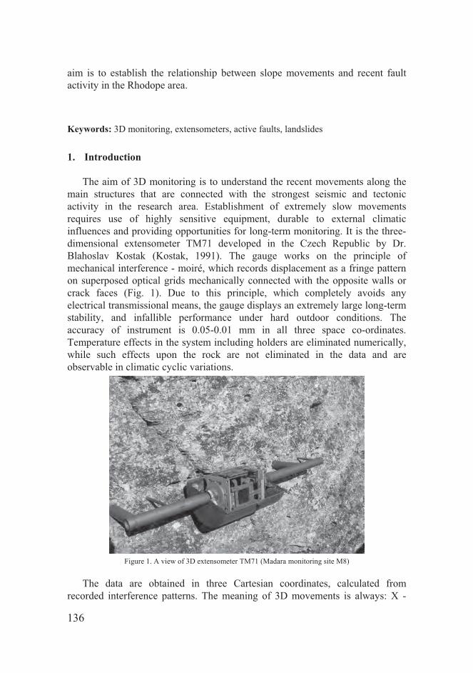
136

aim is to establish the relationship between slope movements and recent fault activity in the Rhodope area.

Keywords: 3D monitoring, extensometers, active faults, landslides

1. Introduction

The aim of 3D monitoring is to understand the recent movements along the main structures that are connected with the strongest seismic and tectonic activity in the research area. Establishment of extremely slow movements requires use of highly sensitive equipment, durable to external climatic influences and providing opportunities for long-term monitoring. It is the three-dimensional extensometer TM71 developed in the Czech Republic by Dr. Blahoslav Kostak (Kostak, 1991). The gauge works on the principle of mechanical interference - moiré, which records displacement as a fringe pattern on superposed optical grids mechanically connected with the opposite walls or crack faces (Fig. 1). Due to this principle, which completely avoids any electrical transmissional means, the gauge displays an extremely large long-term stability, and infallible performance under hard outdoor conditions. The accuracy of instrument is 0.05-0.01 mm in all three space co-ordinates. Temperature effects in the system including holders are eliminated numerically, while such effects upon the rock are not eliminated in the data and are observable in climatic cyclic variations.

Figure 1. A view of 3D extensometer TM71 (Madara monitoring site M8)

The data are obtained in three Cartesian coordinates, calculated from

recorded interference patterns. The meaning of 3D movements is always: X -

137

horizontal, across the contact, Y - horizontal slip, and Z - vertical displacement. The movements are relative between the two sides, presented in graphs as displacements of the lower block on the slope to the opposite one, although the interpolation must consider the movement at both sides. The gauge is used for regular monitoring of slow displacements along active faults, landslide fissures and rock deformations.

Basing on this idea, the monitoring points equipped with precise 3D extensometers TM-71 were created during 1970’s and 1980’s in huge block landslides along Northern Bulgarian Black sea coast (Fig. 2) – at the landslides of Taukliman-Rusalka (3 gauges) and Zlatni Pyasatsi (1 gauge). Later, other polygons for monitoring were arranged in Bulgaria: at Simitli graben, SW Bulgaria (4 gauges), Madara Plateau, NE Bulgaria (3 gauges), and East Rhodope area (2 gauges).

2. Bulgarian Northern Black Sea coast and Madara Plateau

Three plateaux situated in NE Bulgaria named Dobrudja, Frangya and Madara whose peripheral zones are affected by destructive slope processes were firstly involved in the monitoring studies. Three monitoring points in the vast landslide of lateral spread type called Taukliman (Rusalka), and another one in the landslide above the sea-side resort of Zlatni Pyassatzi near Varna City were set up. Later, in 1990 and 1993, three gauges have been installed at the rock scarp of Madara Plateau to detect the deformations concerning

Figure 2. Locations of monitoring polygons in Bulgaria. The locations with numbers are as follows: 1, Taukliman (Rusalka); 2, Zlatni Pyasatsi; 3, Kaliakra; 4, Yaylata

The historical bas-relief Madara Horseman protected by the World Heritage

List of UNESCO. The morphology of these plateaux has been predetermined by their characteristic geological features which can be deduced to the two-layer

138

model (Kamenov and Iliev, 1963). Their upper parts are built by hard brittle rocks, ordinarily limestones or sandstones. Below them underlies a sedimentary complex built by plastic marls and/or clays. The deformations in the plastic layer under weight of the rock complex provokes splitting in the marginal zones of the plateaux and separating of rock blocks (steps, slices).

Taukliman (Rusalka) Landslide affects the NE marginal zone of Dobrudja Plateau, 4 km N of Kaliakra Cape. The higher rock complex is built by Sarmatian limestones thick 40-60 m, and the lower plastic complex is built by Oligocene clays. Seven landslide steps wide 5-20 m are formed. As it is mentioned above, three extensometers are installed: two between the main scarp and the last time formed (uppest) landslide step (called as T1 and T3), and one (T2) between the last and second steps.

In the section between the town of Varna and the village of Kranevo, the Frangya Plateau is built by Sarmatian sediments, too, declined 3-4° to NE (Fig. 3). The higher complex is built by limestones thick 20-25 m. Below them there are fine grained sands and diatomaceous clays. Four landslide cirques along the plateau scarp are formed. At the northest of them (Zlatni Pyasatsi), a single landslide step is formed below the plateau edge. It is wide 3-8 m. The terrain bellow the rock lamella is built by disintegrated rock blocks and mixed landslide materials moving slowly towards the sea shore. In 1981, an extensometer (ZP4) was installed in the fissure between the plateau’s scarp and the separated step.

Results from the monitoring on landslide movements indicates a stable trends of creep of rock blocks to the sea (Fig. 4). Movements have sinusoidal character due to the

Figure 3. Cross section of Zlatni Pyasatsi Landslide: 1, mixed landslide materials; 2, limestones; 3, fine sands; 4, diatomaceous clays; 5, slip surface; 6, location of the monitoring point.

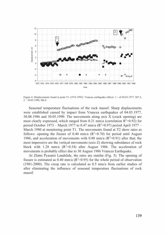
139 139

-6

-4

-2

0

2

4

6

8

10

12

1972 1973 1974 1975 1976 1977 1978 1979 1980 1981 1982 1983 1984 1985 1986 1987 1988 1989 1990 1991 1992

time

disp

lace

men

t, m

m

x y z

1

2

Figure 4. Displacements found at point T1 (1972-1992). Vrancea earthquake effects: 1 - of 04.03.1977, M7.2; 2 – 30.05.1990, M6.8

Seasonal temperature fluctuations of the rock massif. Sharp displacements

were established caused by impact from Vrancea earthquakes of 04.03.1977, 30.08.1986 and 30.05.1990. The movements along axis X (crack opening) are most clearly expressed, which ranged from 0.21 mm/a (correlation R2=0.92) for period October 1973 – March 1977 to 0.47 mm/a (R2=0.97) period April 1977 – March 1980 at monitoring point T1. The movements found at T2 show rates as follows: opening the fissure of 0.40 mm/a (R2=0.70) for period until August 1986, and acceleration of movements with 0.80 mm/a (R2=0.91) after that; the most imperssive are the vertical movements (axis Z) showing subsidance of rock block with 1.28 mm/a (R2=0.54) after August 1986. The acceleration of movements is probably effect due to 30 August 1986 Vrancea Earthquake.

At Zlatni Pyasatsi Landslide, the rates are similar (Fig. 5). The opening of fissure is estimated as 0.40 mm/a (R2=0.95) for the whole period of observation (1981-2000). The creep rate is calculated as 0.5 mm/a from earlier studies of after eliminating the influence of seasonal temperature fluctuations of rock massif.

139

140

-4

-2

0

2

4

6

8

10

1980 1981 1982 1983 1984 1985 1986 1987 1988 1989 1990 1991 1992 1993 1994 1995 1996 1997 1998 1999 2000

time

disp

lace

men

t, m

m

x

y

z

Figure 5. Displacements found at point ZP4 (1981-2000)

The two-layer model of Madara Plateau is characteristic by its higher, Cenomanian, limy-sandstone complex thick 120-140 m, and its lower, Hauterivian, marly complex. The peripheral zone of Madara Plateau is split by rock slices wide 1-3 m and high 80-120 m. The main factors of splitting the rock scarp are the deformations in the lower plastic complex as well as the gravitational extensions of the rock massif (Frangov et al. 1992; Košták et al. 1998).

Three gauges have been installed in Madara area. The monitoring point M9 was arranged in the fissure between the main scarp and the 1st rock slice. Other two points (M8 and M10) were mounted on cracks in frontal part of scarp directly affecting the rock bas-relief. The implemented precise monitoring shows contemporary active movements at the three monitoring points as well as some better or more weakly expressed tendencies (Frangov et al. 1992; Košták et al. 1998). The most impressive movements are established at the plateau edge. A continuous slip movement of the rock slice at a speed of 0.85 mm per year towards SSE (Fig. 6). The vertical movements of the slice are characterized with subsiding with 0.8 mm per year during the period 1990-1999, and a relatively stable state from 1999 up to present. For the past 10 years, a clear trend of compression of the crack has been recorded. This process of compression could be explained as a formation of a new rock slice. The acceleration of the process started in 1999 as an influence of the Izmit (Kocaeli) Earthquake, Turkey, 17.08.1999 (M7.4).

141

-20

-10

0

10

20

30

40

1989 1991 1993 1995 1997 1999 2001 2003 2005 2007 2009 2011

t ime

x

y

z

Vrancea Eart hquakes, M=6.8 and 6.3, 30-31.05.1990

Izmit Eart hquake, M=7.4, 17.08.1999

Provadia Eart hquake, M=4.5,

Figure 6. Displacements found at point M9 (modified after Dobrev, 2010)

3. Simitli graben

The Simitli graben is situated at the crossing point of two significant fault zones called Strouma (local directions 150-170°) and Krupnik-Gradevo (40-60°). A longer part of the graben is formed along the Krupnik-Gradevo fault zone. The research area is the epicentral zone of one of the strongest Balkan and European earthquakes – on 4 April 1904, 10:02 and 10:25 GMT, with magnitudes 7.1 and second one 7.5-7.8, respectively (Christoskov and Grigorova, 1968; Gutenberg and Richter, 1954).

In 1982-1983, three extensometers for three-dimensional monitoring of fault movements were installed in SW Bulgaria: K5 (in Struma Fault inside the Kresna Gorge), B6 (Krupnik fault near Brezhani Village), and K7 (near Krupnik Village – in seismogravitational cracked slope deformation). The last point K12 (in Struma Fault inside the Kresna Gorge) was installed in 2003. Avramova-Tacheva et al. (1984) and Dobrev and Koš ák (2000) have already described the present situation of the monitoring points in detail. The frequency of observation is once monthly or bimonthly, as well as after any stronger earthquake or other event that occurred in the area of study.

Montoring point B6 shows the most impressive results. For the whole period of observation (1982-2010), it is established that the general movements are as follows: extension 1.15 mm/a (R2=0.76), left-lateral slip of 1.88 mm/a (R2=0.94), and a reverse slip of –1.59 mm/a (R2=0.95). Concerning horizontal

142

movements, varying periods of compression and extension at fault are established. The deformation accumulated so far is impressive. The total displacement is 86.81 mm at the end of 2010. The last detailed analysis by Dobrev and Kostak (2000) concerned the period up to May 1999 just before the strong Izmit Earthquake. Despite the great distance from the epicenter (600 km) some major displacements were established. It was found that the movements had fluctuation character along the fault. These were so intense that the apparatus was seriously damaged. The average resulting displacements during seismic vibrations were calculated as follows: ΔX=–8.34 mm (compression), ΔY=–5.09 mm (right-lateral slip), and ΔZ=–0.96 mm (thrusting).

Fig. 7. A photograph of monitoring point B6. The left-lateral displacement of steel holders is obvious (after Dobrev, 2011).

Monitoring point K5 (Kresna Gorge, Struma Fault Zone) is characteristic

with high amplitudes due to the direct atmospheric impact on the gauge. For the whole period (1982-2010), a general direction of extension of the zone has been established. The general movements are as follows: extension 0.10 mm/a (R2=0.58), left-lateral slip of 0.28 mm/a (R2=0.78), and a subsidence of SW block (probably reverse) of 0.11 mm/a (R2=0.62). Since 1998, the rate of movement is left-lateral ranging from 0.4 to 0.8 mm/a.

Monitoring point K12 (Struma Fault Zone) was installed in November 2003. Seven periods of movement are distinguished (Dobrev, 2011). In the first period some sharp displacements at Y- and Z-axes are established (Fig. 8). Movements of a sharp left displacement ( Y=–3.34 mm) and a thrusting ( Z=–3.79 mm) have been recorded, which coincide with a local earthquake swarm. However, the most interesting is the period from January to October 2006 revealing a clear vertical movement along the fault. This is a typical creep, initially starting with a slow movement (0.91 mm/a) from January to late May, and after that begins an

143

acceleration of the motion with a constant velocity ~7 mm/a. Interesting is the stable velocity of this creep. During this period there is a hard seismic activity, starting from early February to early June 2006 in the west and northwest of the Struma fault zone. These are earthquakes in the territories of Bulgaria and FYR of Macedonia. The strongest of them occurred in Macedonia with M=3.7.

Figure 8. Displacements found at point K12 (Dobrev, 2011)

The whole monitoring period 2003-2010 is characteristic by extension of

zone of 0.08 mm/a, left-lateral slip of -0.09 mm/a, and a reverse slip of 0.72 mm/a.

4. East Rhodope area

In 2001, a system of fault surfaces revealed after a landslide triggering near the village of General Geshevo (in the vicinity of Djebel Town, East Rhodopes Mts.). The field research of neighbouring areas confirmed the presence of a large fault zone following a direction of 130° with distribution of multiple slope processes. Because this region is poorly studied from the engineering geological and tectonic point of view, the question of a new view of geodynamics in the region and its impact on the development of landslide phenomena took place. Here are developed the deepest landslides in Bulgaria. Landslides around Djebel Town have sizes of several hundreds meters to several kilometers, and their volumes often reach to hundreds of millions of cubic meters. The geological structure in the reseach area is represented by Paleogene volcano-sedimentary complex including tuffs, zeolites, rhyolites, sands and clays.

The monitoring here is organized at two main locations as follows:

144

• Chamurdjuk (Karaboruntepe) location: 1 extensometer TM71 (point GG11) and 4 shift marks. All points are located outside the landslide body, near to main scarp.

• Location at shear zone near Jaladovo Village (over 500 m far from the landslide, at the road between villages of General Geshevo and Ustren): 1 extensometer TM-71 (point J13, see Fig. 9) and 1 shift mark. The results obtained at first location show decreasing slope movements. Two

stages are found at extensometric point GG11 up to present: The first one is from July 2003 to August 2004, and the second one is from 2005 till present. In the first stage, the movements follow the direction of sliding movement with a rate of 2.64 mm per year; during the second stage the slip decrease to 0.54 mm per year.

Fugure 9. The newest extensometric point J13 near Jaladovo Village installed in 2010 (Krastanov et al., 2010)

On 8 September 2008, sharp movements (exceeding 20 mm at some spatial

axes) have been recorded at two, which are followed by compensation with the same size. We explain this phenomenon by overall movement of landslide masses followed by compensatory movements of approximately equal value (Krastanov et al., 2010).

5. Discussion

The use of 3D in-situ monitoring with TM-71 extensometer is a successful approach to identifying the dynamics of the geological hazards. The other methods of monitoring establish rates of tectonic and landslide movements, which are often controversial due of the accuracy of measurements. The

145

advantage of this technique is that it is purely mechanical, less influenced by atmospheric impact and its maintenance is easier.

Interesting results were obtained from direct measurements with this gauge in Bulgaria. Different periods of movements, creep, and sharp jumps of co-seismic character have been established. The most representative are the results of the monitoring of active faults in SW Bulgaria. A new statistical approach found anormalies in movements 2-3 months before earthquakes in Northern and Central Greece (Shanov, 1993; Shanov and Dobrev, 1997). This method could be applied to other monitoring points in Bulgaria, such as the Northern Black Sea coast or the Madara plateau. To obtain more representative results, it is wishful to enlarge and support a stable and regularily functioning monitoring network in Bulgaria.

Acknowledgements

Th present study was implemented thanking to financial support from the Ministry of Education, Youth and Science of Bulgaria within frames of cooperation projects NZ-635, NZ-1211Gc, NZ-1316 and BIn-09/11, and under long-term cooperation with IRSM, Prague.

References:

Avramova-Tacheva, E., Vrablyanski, and B. Košták. 1984. An attempt to detect recent movements along seismogenic faults. Review of the Bulgarian Geological Society, vol. XLV, part 3, 276-288 (in Bulgarian).

Dobrev N. 2010. In-situ monitoring of cracks affecting the Madara Horseman historical rock monument, Northeastern Bulgaria. First Int. Congress on applied geology, Mashhad, Iran, 26-28 Apr. 2010.

Dobrev, N. 2011. 3D monitoring of active fault structures in the Krupnik-Kresna seismic zone, SW Bulgaria. Acta Geodyn. Geomater., Vol. 8, No. 4 (164), 1–12 (in print).

Dobrev, N.D. and B. Kostak. 2000. Monitoring tectonic movements in the Simitli Graben, SW Bulgaria. Engineering Geology, Elsevier, 57 (3-4), 179-192.

Dobrev, N., E. Avramova-Tacheva and B. Koš ák. 2008. The monitoring of cracks affecting the Madara Horseman bas-relief. Int. Conf. Geoarchaeology and Archaeomineralogy, Sofia, 29-31 Oct., 385-390.

Gutenberg, B. and C Richter. 1954,: Seismicity of the Earth and Associated Phenomena. Princeton University Press, 310 pp.

Christoskov, L. and E. Grigorova. 1968. Energetic and space-time characteristics of the destructive earthquakes in Bulgaria after 1900. Bull. Geophys. Inst., BAS, 12, 79-105 (in Bulgarian).

Frangov, G., P.Ivanov, N.Dobrev and I.Iliev. 1992. Stability problems of the rock monument "Ma-dara horseman". Proc. of the 7th Int. Cong. on Deterioration and Conserv. of Stone, Lisboa, Portugal: 1425-1435.

Kamenov, B. and I.Iliev 1963. Engineering-geological zoning of Bulgaria. Works on the Geology of Bulgaria, Ser.Eng.Geol.& Hydrogeol., 2: 5-123 (in Bulgarian).

Koš ák, B. 1991. Combined indicator using moiré technique. Proc. 3rd Int. Symp. Field Measurements in Geomechanics, Oslo, 53-60.

146

Kostak, B., N.Dobrev, P.Zika and P.Ivanov. 1998. Joint monitoring on a rock face bearing an historical bas-relief. Quarterly Journal of Engineering Geology, London 30(1), 37-46.

Krastanov M., N. Dobrev and A. Pandey. 2010. Monitoring on landslide and possible fault movements near to villages General Geshevo and Zheladovo, East Rhodope Mts. Engineering Geology and Hydrogeology, 25, 99 - 122 (in Bulgarian).

Shanov, S. 1993. Medium-time earthquake prediction based on tectonic fault zone displacement data. Acta Montana, Praha, Series A, No.4(90), 52-62.

Shanov, S.B. and N.D. Dobrev. 1997. Impact of the seismic processes on the movements along the Kroupnik fault zone (SW Bulgaria). Comptes rendus de l'Academie bulgare des Sciences, 6, 95-98.

147

ACTIVITIES IN KARST OF SLOVENIA RELATED TO EARTHQUAKE

PRECOURSORS

SHORT TITLE: ACTIVITIES IN KARST STANKA ŠEBELA*, JANEZ MULEC ZRC SAZU, Karst research institute, Titov trg 2, 6230 Postojna, Slovenia

*To whom correspondence should be addressed. Stanka Šebela, ZRC SAZU, Karst Research Institute, Titov trg 2, 6230 Postojna, Slovenia; e-mail: sebela@zrc-sazu.si

Abstract. Four activities related to the monitoring of earthquake precursors are presented in the paper. TM 71 extensometer monitoring is carried out in four karst caves in Slovenia and also in one artificial tunnel that leads to the fifth karst cave. In Postojna Cave automatic data readings each 15 minutes are organized. In othe caves data are taken manually. Relative micro-displacements in 3D are detected and periods that coincide with local earthquakes are studied for example of Kostanjevica Cave. The 2D displacements of static vertical pendulum in Magdalena Cave are registered each 10 seconds. Solar panel was settled outside the cave to provide the on-line data transfer. Two different methods (TM 71 extensometers and pendulum) are showing interesting comparative results inside the same cave system. The TM 71 gives long-term view of micro-deformations and pendulum gives short-term view. The studies are oriented towards the aim to connect the periods of micro-displacements with local and worldwide seismicity. The third activity represents the temperature monitoring of two sulphidic waters. The natural sulphidic spring Žveplenica in NW Slovenia is situated only some 10 meters south of Dinaric oriented (NW-SE) Kobarid Fault and 2.3 km south of regionally important Idrija Fault in coarse-grained massive Upper Triassic dolomite with tectonic situation typical for External Dinarides. Sovra Valley well gives constant discharge of 15 L per minute with dissolved sulphide. It is located within the Ravne Fault (NW-SE), which was responsible for M=5.6 earthquake in 1998 and for M=5.2 earthquake in 2004. Temperature changes are interesting, because there are periods with stable temperature and periods with higher temperature changes not directly linked to seasonal influences. More data are needed to indicate these parameters as possible earthquake precursor signals. Microbiological monitoring site was established on the fault planes in Postojna Cave at the TM 71 extensometer monitoring site to find the possible connection between microbial biomass and tectonic displacements.

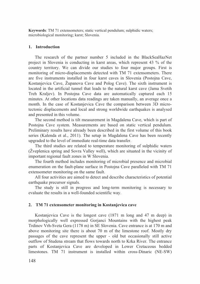
148

Keywords: TM 71 extensometers; static vertical pendulum; sulphidic waters; microbiological monitoring; karst; Slovenia.

1. Introduction

The research of the partner number 5 included in the BlackSeaHazNet project in Slovenia is conducting in karst areas, which represent 43 % of the country territory. We can divide our studies to four major groups. First is monitoring of micro-displacements detected with TM 71 extensometers. There are five instruments installed in four karst caves in Slovenia (Postojna Cave, Kostanjevica Cave, Županova Cave and Polog Cave). The sixth instrument is located in the artificial tunnel that leads to the natural karst cave (Jama Svetih Treh Kraljev). In Postojna Cave data are automatically captured each 15 minutes. At other locations data readings are taken manually, an average once a month. In the case of Kostanjevica Cave the comparison between 3D micro-tectonic displacements and local and strong worldwide earthquakes is analysed and presented in this volume.

The second method is tilt measurement in Magdalena Cave, which is part of Postojna Cave system. Measurements are based on static vertical pendulum. Preliminary results have already been described in the first volume of this book series (Kalenda et al., 2011). The setup in Magdalena Cave has been recently upgraded to the level of immediate real-time data transfer.

The third studies are related to temperature monitoring of sulphidic waters (Žveplenica spring and Sovra Valley well), which are situated in the vicinity of important regional fault zones in W Slovenia.

The fourth method includes monitoring of microbial presence and microbial enumeration on the fault-plane surface in Postojna Cave paralleled with TM 71 extensometer monitoring on the same fault.

All four activities are aimed to detect and describe characteristics of potential earthquake precursor signals.

The study is still in progress and long-term monitoring is necessary to evaluate the results in a well-founded scientific way.

2. TM 71 extensometer monitoring in Kostanjevica cave

Kostanjevica Cave is the longest cave (1871 m long and 47 m deep) in morphologically well expressed Gorjanci Mountains with the highest peak Trdinov Vrh-Sveta Gera (1178 m) in SE Slovenia. Cave entrance is at 170 m and above monitoring site there is about 70 m of the limestone roof. Mostly dry passages of the cave represent the upper - old but occasionally still active outflow of Studena stream that flows towards north to Krka River. The entrance parts of Kostanjevica Cave are developed in Lower Cretaceous bedded limestones. TM 71 instrument is installed within cross-Dinaric (NE-SW)

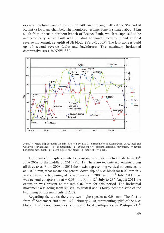
149

oriented fractured zone (dip direction 140° and dip angle 80°) at the SW end of Kapniška Dvorana chamber. The monitored tectonic zone is situated about 3 km south from the main northern branch of Brežice Fault, which is supposed to be neotectonically active fault with sinistral horizontal movement and vertical reverse movement, i.e. uplift of SE block (Verbi , 2005). The fault zone is build up of several reverse faults and backthrusts. The maximum horizontal compressive stress is NNW-SSE.

Figure 1. Micro-displacements (in mm) detected by TM 71 extensometer in Kostanjevica Cave, local and worldwide earthquakes. (+ x – compression, - x – extension; + y – sinistral horizontal movement, - y dextral horizontal movement; + z – down-slip of NW block, - z – uplift of NW block).

The results of displacements for Kostanjevica Cave include data from 17th

June 2008 to the middle of 2011 (Fig. 1). There are tectonic movements along all three axes. From 2008 to 2011 the z-axis, representing vertical movements, is at + 0.03 mm, what means the general down-slip of NW block for 0.03 mm in 3 years. From the beginning of measurements in 2008 until 12th July 2011 there was general compression at + 0.03 mm. From 12th July to 23rd August 2011 the extension was present at the rate 0.02 mm for this period. The horizontal movement was going from sinistral to dextral and is today near the state of the beginning of measurements in 2008.

Regarding the z-axis there are two highest peaks at 0.04 mm. The first is from 7th September 2009 until 12th February 2010, representing uplift of the NW block. This period coincides with some local earthquakes as Postojna (15th

150

January 2010, M=3.7), Gorjanci Mountain (21st January 2010, M=3.2) and Kostanjevica (28th February 2010, M=2.8). Postojna town is 90 km to the West from the TM 71 monitoring site in Kostanjevica Cave. Gorjanci Mountain and Kostanjevica town are only some km away from the monitoring site.

The second peak on z-axis at + 0.04 mm was down-slip of NW block (7th May - 25th July 2010) coinciding with Gorjanci Mountain local earthquake on 3rd July 2010 (M=1.9).

The third highest peak on z-axis was from 11th April to 7th May 2010 at - 0.03 mm (uplift of NW block).

The y-axis does not show significant movement in a general sense for the studied period (2008-2011), but short-term periods show more activity. From 20th December 2008 until 5th April 2009 there was dextral horizontal movement at – 0.03 mm, which coincided with Brežice (6th February 2009, M=2.5) and Metlika (16th February 2009, M=2.1) earthquakes. Brežice town is situated 15 km to the East and Metlika town is 20 km SW from the TM 71 monitoring site. After that period, starting from 5th April 2009 until 7th June 2009, there was significant (+ 0.025 mm) sinistral movement. This coincides with Aquila earthquake in Italy (6th April 2009, M=6.3).

From 23rd November 2010 to 12th April 2011 there was dextral horizontal movement at – 0.025 mm, followed by sinistral horizontal movement at + 0.01 mm (12th April to 12th July 2011). This period can be related to Žužemberk (10th June 2011, M=2.4) and Raka (20th August 2011, M=3.1) earthquakes. Žužemberk is situated 35 km to the West and Raka 10 km to the North from TM 71 monitoring site.

The x-axis established compression from 17th June 2008 to 25th July 2010 at + 0.04 mm and extension at – 0.03 mm from 25th July 2010 to 23rd August 2011.

Monitoring of tectonic displacements in Kostanjevica Cave is interesting for understanding the active tectonic conditions in Krško valley and Gorjanci Mountain area, as well as for active deformations of the location of Krško nuclear power plant being 13 km to the north from TM 71 monitoring site in Kostanjevica Cave.

3. Static vertical pendulum in Magdalena Cave

Preliminary results of tilt measurements in Magdalena Cave in Slovenia have already been described (Kalenda et al., 2011). The pendulum is in operation from 1st July 2010. In October 2011 the setup has been upgraded to the level of immediate real-time data transfer. The results are showing increase of noise before bigger worldwide earthquakes. Deformations before bigger earthquakes were detectable in Magdalena Cave by a static vertical pendulum.

151

4. Temperature monitoring of sulphidic waters

The sulphidic spring Žveplenica in Dolenja Trebuša (Fig. 2) is situated only

some 10 meters south of Dinaric oriented (NW-SE) Kobarid Fault and 2.3 km south of regionally important Idrija Fault in coarse-grained massive Upper Triassic dolomite with tectonic situation typical for External Dinarides.

Figure 2. Structural geological position of two studied sulphidic waters in W SloveniThe spring discharge was rather constant in 2-year (2009-2010) monitoring period, approximately 1.8 L/min. Average temperature was 10.5 ± 0.2 oC, with an average pH of 7.56 ± 0.12, and specific conductance of 419 ± 9 S/cm. Measurements at the spring orifice showed low concentration of dissolved oxygen (0.13 mg/L). Dissolved sulphide concentration was 7.8 mg/L, sulphate 9.9 mg/L, and nitrate and ammonium 0.0 mg/L. Temperature changes are interesting, because there are periods with stable temperatures and periods with higher temperature changes (Fig. 3).

Figure 3. Temperature changes at Žveplenica sulphidic spring.

152

The second monitoring site with sulphidic water (0.16 mg of H2S per litre) is

Sovra Valley well situated near the Ravne Fault (Fig. 2). Seismic activity along this fault was responsible for M=5.6 earthquake in 1998 and for M=5.2 earthquake in 2004. The temperature is much more stable at Sovra (temperature changes <0.01 °C in July-September 2009) as it is at Žveplenica.

To better understand possible earthquake precursor signals we need to continue with temperature monitoring at both locations and make additional chemical analyses of sulphidic waters. There is also the need to connect seismological data from local earthquakes (magnitude, depth etc.) with periodical temperature changes of studied sulphidic waters.

5. Microbiological monitoring

The objective of this activity was to test efficiency and sensitivity of RIDA®COUNT test kits (R-Biopharm AG, Germany, http://www.r-biopharm.com/) on a fault surface in Postojna Cave at the site of TM 71 extensometer monitoring. This kit was already successfully tested in karst caves in Slovenia and Slovakia for monitoring of organic loads by detecting cultivable microorganisms in various habitats; water, air and on solid surfaces (Mulec et al., 2012). By sampling of surface swabs on the fault zone we wanted to observe how fast this fault plane can conduct “microbial flow” from upper laying limestone layers (58 m) due to gravity to the underground cave system (Fig. 4). On this fault plane seeping water is occasionally present. On the fault zone we took swabs prior and after surface sterilization.

153

Figure 4. Schematic representation of the swab sampling site at the fault zone where TM71 is installed in Postojna Cave in the section named Lepe jame.

For surface swab sampling to observe viable microbial counts we used RIDA®COUNT test plates: RIDA®COUNT Total for total aerobic count, RIDA®COUNT Coliform for total count of coliform bacteria, and RIDA®COUNT Yeast&Mold Rapid for counts of fast growing yeasts and moulds (Mulec et al., 2012). Fault surface was sampled twice prior surface sterilization and five times after sterilization. Preliminary results showed that cultivable bacteria were detected on the fault surface after four months, yeast and moulds after three months. Coliform bacteria were never detected on the surface. On the fault surface we observed increasing trend of total microbial counts (bacteria, yeast and moulds) after surface sterilization (Fig. 5). Nevertheless, microbial counts on the surface are sum of cultivable microorganisms, which came from the karst surface and beneath lying layers, and airborne microbiota. From previous studies (data not shown) we know that this particular site is very poor in airborne microorganisms, that is why most of the detected microorganisms came along the fault zone from the upper layers with seeping water (influence of precipitation, Fig. 5). Results indicated that fault zones can be good conductors for particles of micrometer sizes due to gravity. It is worth to mention from other studies that fault can represent extremely heterogeneous habitat for microorganisms and seismic activities might produce habitable space for microbial life and supply of nutrients (Kaksonen and Inagaki, 2008).

154

Figure 5. Column chart represents on primary vertical axes precipitation in Postojna (Postojna Cave) in the period from 15 June 2010 till 15 January 2011 (source: Slovenian Environmental Agency). Microbial counts of bacteria, yeast and fungi per surface unit expressed as colony-forming units CFU per 100 cm2 are indicated on secondary vertical axes (dots). An arrow represents the date (14 July 2010) of surface sterilization at the sampling site of the fault zone.

6. Conclusions

There are four activities going on related to karst areas in Slovenia. First is 3D micro-tectonic monitoring with TM 71 extensometers the second is 2D measurements of tilt and noise in Magdalena Cave by a static vertical pendulum. The third activity includes temperature monitoring of two sulphidic waters, and the fourth activity represents microbiological monitoring of the fault plane surface.

There are five TM 71 extensometer instruments installed in karst caves in Slovenia (Postojna Cave, Kostanjevica Cave, Županova Cave and Polog Cave). The sixth instrument is located in artificial tunnel that leads to the natural karst cave (Jama Svetih Treh Kraljev). For this volume the data from Kostanjevica Cave of 3D micro-displacements (2008-2011) are presented.

There are tectonic movements along all three axes. From 2008 to 2011 the z-axis, representing vertical movements, is at + 0.03 mm, what means the general down-slip od NW block for 0.03 mm in 3 years. From the beginning of measurements in 2008 until 12th July 2011 there was general compression at + 0.03 mm. From 12th July to 23rd August 2011 the extension was present at the rate 0.02 mm for this period. The horizontal movement was going from sinistral to dextral and is today near the state of the beginning of measurements in 2008.

There are some periods where micro-displacements coincide with local earthquakes. The best examples are related to Brežice and Metlika earthquakes in 2009 (y-axis, dextral horizontal movement at – 0.03 mm), to Postojna,

155

Gorjanci and Kostanjevica earthquakes in 2010 (z-axis, uplift of NW block for 0.04 mm), and to Žužemberk and Raka earthquakes in 2011 (y-axis, dextral horizontal movement at – 0.025 mm, followed by sinistral horizontal movement at + 0.01 mm).

Static vertical pendulum in Magdalena Cave was described in detail in the first volume (Kalenda et al., 2011). There are data of the development of tilt and nose starting from 1st July 2010 until present. Since October 2011 the realization of the transfer of data in real-time was a big success for our research.

Two different methods (TM 71 extensometers and static vertical pendulum) are showing interesting comparative results. The TM 71 gives long-term view of micro-deformations and pendulum gives short-term view. The studies are oriented towards the aim to connect the periods of micro-displacements detected by TM 71 extensometers and pendulum with local and worldwide seismicity.

Both sulphidic water locations are interesting because of their geological position near likely active Dinaric (NW-SE) faults in W Slovenia. At Žveplenica sulphidic spring we continue with long-term temperature monitoring. To get better insight into dynamics of the spring and eventual link to seismic activities, additional measurements of other physical and chemical parameters are needed.

Preliminary results of microbiological indicators (bacteria, yeast and fungi) showed that fault plane play an important role in material transport between external surface and upper layers with the underground voids in relatively short time. Longer monitoring is needed to find possible connections between tectonic activity on the studied fault-plane in Postojna Cave and microorganisms.

ACKNOWLEDGEMENT The study started in 2004 within the COST 625 project (3D monitoring of active tectonic structures) and is continuing within Slovenia-Czech bilateral projects (BI-CZ/06-07-011 and BI-CZ/08-09-015), FP7-INFRA-2010 Preparatory Phase Project EPOS (European Plate Observing Systems) and FP7-PEOPLE-2009-IRSES-246874 (BlackSeaHazNet-Complex Research of Earthquake's Prediction Possibilities, Seismicity and Climate Change Correlations).

156

References

Briestenský, M. and Stemberk, J., 2007, Recent displacements registered in selected caves of

Dobrá Voda karst area in Slovakia. Acta Geodyn. Geomater. 4(1):31-38. Gosar, A., Šebela, S., Koš ák, B. and Stemberk, J., 2009, Surface versus underground

measurements of active tectonic displacements detected with TM 71 extensiometers in Western Slovenia. Acta Carsologica. 38(2-3):213-226.

Gosar, A., Šebela, S., Koš ák, B. and Stemberk, J., 2011, On the state of the TM 71 extensometer monitoring in Slovenia: seven years of micro-tectonic displacement measurements, Acta Geodyn. Geomater. 8(4):1-6.

http://www.r-biopharm.com/ Kaksonen, A.H., Inagaki, F. 2008, Distribution of microbial life in marine subsurface sediments of

the seismigenic subduction zone. In: Kato K., Kimura H. (Eds.), 7th International Symposium for Subsurface Microbiology, Shizuoka, Japan, November 16-21, 2008, Shizuoka, 143.

Kalenda, P., Koš ák, B., Stemberk, J., Neumann, L. and Šebela, S., 2011, Micro-tectonic movements in karst caves (Slovenia) as indicators of Earth’s stress changes – earthquake precursor implications. BlackSeaHazNet Series, vol 1, BlackSeaHazNet Methodological – Coordination Workshop, 2-5 May 2011, Ohrid, pp. 159-173.

Koš ák, B., Caco , S., Dobrev, N., Avramova-Ta eva, E., Fecker, E., Kopecký, J., Petro, L., Schweitzer, R. and Nikonov, A., 2007, Observations of tectonic microdisplacements in Europe in relation to the Iran 1997 and Turkey 1999 earthquakes. Izvestiya, Physics of the Solid Earth, 43:503-516.

Mulec J., Krišt fek V. and Chro áková A. 2012, Comparative microbial sampling from eutrophic caves in Slovenia and Slovakia using RIDA®COUNT test kits. International Journal of Speleology, 41 (1):1-8.

Stemberk, J., Koš ák, B. and Cacon, S., 2010, A tectonic pressure pulse and geodynamic activity recorded from long-term monitoring of faults in Europe. Tectonophysics, 487(1-4):1-12.

Šebela, S., Koš ák, B. and Stemberk, J., 2010, Recent micro-tectonic movement from three karst caves, Slovenia. Scientific Annals, School of Geology, Aristotle University of Thessaloniki, Proceedings of the XIX CBGA Congress, Thessaloniki, Greece, special volume 99/1, pp. 513-518.

Verbi , T., 2005, Quaternary stratigraphy and neotectonics of the Eastern Krško basin, Part 2: Neotectonics. Razprave IV. Razreda SAZU, XLVI(1):171-216.

157

DFA ANALYSIS OF SEGMA MAGNETIC FIELD DATA AROUND THE

M6.3 AQUILA EQ

P. NENOVSKI1, M. CHAMATI1, U. VILLANTE2, M. DE LAURETIS2, M. VELLANTE2, P. FRANCIA2, V. WESZTERGOM3, K. SCHWINGENSCHUH4, M. BOUDJADA4, G. PRATTES4

1National Institute for Geophysics, Geodesy and Geography, Sofia, Bulgaria.2Dipartimento di Fisica, L’Aquila Università, L’Aquila, Italy.3Geodetic and Geophysical Research Institute, Sopron, Hungary. 4Institut für Weltraumforschung, Graz, Austria.

Address: pnenovski@geophys.bas.bg

Abstract. Recently a preliminary analysis of the magnetic field observations performed at L’Aquila preceding the April 6, 2009 earthquake has been performed (Villante et al, 2010). A possible occurrence of features as i) an increase in the noise background and/or polarization parameter (i.e. the ratio between the amplitude/power of the vertical component and that one of the horizontal component), ii) changing characteristics of the slope of the power spectrum and fractal dimension, and iii) occurrence of short duration pulses have been looked for two years back. It was concluded that the expected ULF disturbances related to earthquakes (if any) are generally weak and sophisticated signal processing methods and a lot of experience are required to evaluate the source of ULF emissions observed at ground. In this report we apply detrended fluctuation analysis (DFA) analysis on fluxgate and search-coil data in ULF range (periods 10-90 sec) for months January-April 2009 available from SEGMA array (Italy, Hungary, Austria and Bulgaria). Remind DFA is a data processing method that allows for the detection of scaling behaviors in observational time series even in the presence of non-stationarities. H and Z magnetic field components at night hours (00-03 UT, 01-04 LT) and their variations at stations AQU, CST, NCK and PAG have been examined and their scaling properties are analyzed depending on geomagnetic and local conditions. As it is expected, the DFA scaling exponents increase when Kp index increases, indicating a good correlation with geomagnetic activity. DFA scaling exponent reveals also local changes –such as a considerable decrease for the H component at AQU station observed in the midst of February. A malfunction of the fluxgate magnetometer at Aquila has been checked up and excluded. Attempts to explain thoroughly this unique feature with artificial and/or natural sources including the

158

enhanced earthquake activity occurred in months January-April 2009 at Aquila district are made.

Keywords: magnetic field, DFA scaling exponent, fluctuation function, earthquake,

1. Introduction

Magnetic field data and especially those of 1 second resolutions, are well exploited toward searching any seismogenic signatures preceding incoming earthquakes (EQ). Magnetic field variations in the ULF range (0.003-3 Hz) have been studied around series of strong earthquakes and subsequently underwent hot debates about their authenticity and reliability. Performing ULF observations many authors have applied standard and elaborated signal processing methods to magnetic field data to possibly extract seismogenic electromagnetic ULF emission (Fraser-Smith et al., 1990; Molchanov et al., 2002; Kopytenko et al., 2004; Hayakawa et al., 1996; Hayakawa et al., 2007).

In this paper we draw attention to magnetic field data measurements around the Mw6.3 L’Aquila earthquake occurred on 6 April 2009 in Central Italy. Our preliminary results based solely on magnetic field data at L’Aquila observation did not reveal reliable signatures to be associated with the earthquake (see Villante et al, 2010). The only exception was an appearance of intense spikes of ~1 nT magnitude registered 19 days prior to EQ main shock. The next step is to use all SEGMA magnetic field data collected at the five observatories and stations. Remind that the SEGMA observatories are L’Aquila (AQU), Ranchio (RNC), Castello Tesino (CST), in Italy, Nagycenk (NCK), Hungary, Panagyurishte (PAG), Bulgaria which are evaluated in the frame of this work. Stations Ranchio (RNC), Castello Tesino (CST) and Nagycenk (NCK) are equipped with only fluxgate magnetometers developed at the Space Research Institute of the Austrian Academy of Sciences Graz. The observatories L’Aquila, Italy and Panagyurishte, Bulgaria are equipped both with fluxgate and searchcoil magnetometers.

At the beginning the instrumental characteristics of the magnetometers are described. The CHIMAG fluxgate magnetometer was originally developed at the Space Research Institute of the Austrian Academy of Sciences Graz, to investigate magnetic pulsations in the ULF range. The vital parameters of the high temporal resolution 3-axes fluxgate magnetometer are the measurement range of +/- 512 nT, the compensation field of 60000 nT in X and Z and +/- 30000 nT in Y direction. The accuracy is 8 pT at a temporal resolution of 1 Hz, derived from the highest possible sampling frequency of 64 Hz. The 3-axes magnetometer measures in X (positive Northward), Y (positive Eastward) and Z (positive towards the centre of the Earth) direction. The CHIMAG

159

magnetometer comes to application in the frame of the SEGMA project (see http://sole-terra.aquila.infn.it/staz_segma.asp).

At L’Aquila the fluxgate magnetometer has a rms instrumental noise of ~ 20 pT in the frequency band 1-500 mHz; more specifically, according to the usual classification scheme for continuous pulsations (Pc1: 200-500 mHz; Pc2: 100-200 mHz; Pc3: 20-100 mHz; Pc4: 7-20 mHz; Pc5: 1-7 mHz), the rms noise is ~10 pT (Pc1 band), ~10 pT (Pc2), ~10 pT (Pc3), ~5 pT (Pc4), ~3 pT (Pc5). The rms of the quantization noise is ~0.3 pT. The induction magnetometer has an amplitude/frequency response almost linear (~ 6 Volt/nT/Hz) in the frequency range 0-0.2 Hz. The rms instrumental noise is ~1 pT (Pc1), ~1 pT (Pc2), ~3 pT (Pc3), ~5 pT (Pc4), ~10 pT (Pc5). The rms of the quantization noise is less than 0.5 pT in the frequency range 1-500 mHz.

The fluxgate magnetometer installed at the Panagyurishte observatory is of type MAGSON (MAGSON GmbH–Germany) and performs absolute measurements (see http://www.geophys.bas.bg/geomagn/equip.htm). The characteristics of the searchcoil magnetometer at Panagyurishte (courtesy of the L’Aquila University) are somewhat different from those at L’Aquila. By applying the transfer functions of the two searchcoil magnetometers we are able to interrelate quantitatively magnetic field variations at L’Aquila (Italy) and Panagyurishte (Bulgaria).

2. Scientific background, methodology and data analysis

Previous experience showed that night time magnetic field data are less influenced by man made and geomagnetic effects than day time hours, although the latter cannot be excluded in full. For that reason we extract only the local midnight period from 01:00–04:00 LT (UT + 1) and divide this 4 hour period into 8 half hour intervals equally distributed.

DFA is a well-established method for determining data scaling (self similarity) behavior in the presence of possible trends without knowing their origin and shape (Kantelhardt et al, 2001). In difference to conventional, e.g. power spectrum analysis, the DFA permits detection of intrinsic dynamical features, e.g. long-range correlations, embedded in non-stationary time series and avoid spurious detection of apparent scaling, which may be an artifact of non-stationary time series (Buldyrev et al., 1995). For long-range correlated signals the fluctuation function would behave as a power-law of the time scales, thus its slope should be constant and usually denoted by α index.

It was already indicated that the DFA indices of the vertical Z and horizontal H components of the Earth’s magnetic field vary in similar way. The similarity in Z and H components and in all stations indicate that the source of long-range interactions in the magnetic field data can be associated to magnetospheric/ionospheric sources (Nenovski et al, 2007; Chamati et al, 2010).

160

Shortly, DFA operates on a time series x(i), where i = 1,2,…N and N is the length of series. Next, the integrated series is divided into Ns = int(N/s) non-overlapping segments of equal length s. Since the length N of the series is often not a multiple of the considered time scale s, a short part at the end of the profile y(i) may remain. In order not to miss this part of the series, the same procedure is repeated starting from the opposite end. Thereby, 2 Ns segments are obtained altogether. The local trend for each of the 2 Ns segments is calculated by a least square fit of the series. Then we determine the variance for each segment ν, ν = 1,…, Ns and for ν, ν = Ns+1,…, 2 Ns.

Here, yν(i) is the fitting line in segment ν. After averaging over all segments we derive the fluctuation function F(s). Repeating this procedure for several time scales, F(s) will increase with increasing s. And analyzing log-log plots F(s)-s the scaling behavior of the fluctuation function will be determined. If the series x(i) is long-range power–law correlated, the fluctuation function F(s) will increase for large values of s as a power-law. The value of the slope α resulting from a least-square fit to a straight line, reveals a presence, or not, of long-range correlations. In particular, the case α = ½ represents the absence of long-range correlations.

On the other hand, by applying standard spectral analysis techniques to x(i), the power spectra, i.e. to the square of the Fourier transform amplitudes for x(i), yields exponent β. The power spectral density (PSD) exponent β is related to the DFA scaling exponent α by β = 2α −1.

3. Results

DFA analysis was performed on all available data at AQU, CST, NCK and PAG. Station RNC was out of work in 2009 several months and therefore has been ignored for the present analysis. In general the DFA scaling exponent varies in similar way at all stations and follows closely the geomagnetic activity index Kp (see Chamati et al 2009). Because of conciseness these results are not shown here. Figure 1 and Table display the DFA scaling exponent variations of X and Z components at L’Aquila. As it can be seen, the DFA scaling exponent of the Z and H components which is a measure of the slope of fluctuation in the ULF range (10-90 seconds) showed unusual irregular trends (marked by ellipses) at L’Aquila in February 2009 – approximately two months before the EQ main shock. The DFA scaling exponent revealed an abnormal behavior of nearly a week duration both in vertical Z and horizontal components (X, Y). This event starts on 11 February and disappears completely on 20 February 2009. We found a significant increase of DFA scaling exponent in Z component, followed by significant decrease of this exponent in the horizontal components. These changes are local, they were observed only at L’Aquila.

161

Fig. 1 Table DFA scaling exponents α /searchcoil data/

2007

Jan-Apr 2008 Jan-Apr

2009 Jan-Apr

2010 Jan-Apr

X 0.61±0.17 0.675±0.15 0.581±0.10 0.60±0.10 Z 0.66±0.13 0.72±0.11 0.65±0.08 0.65±0.08

In order to check any possible instrumental influences we drew fluxgate data from the INGV observatory at L’Aquila (http://roma2.rm.ingv.it/it/risorse/banche_dati/39/osservazioni_relative_al_sisma_del_6-4-2009_a_l-aquila). This magnetic observatory is housed at a distance ~200 m from the L’Aquila University observatory. Dynamic spectra of the two fluxgate data reveal identical trends on the interested date (midst of February). So, a malfunction of the fluxgate magnetometer at L’Aquila and its acquisition system is excluded. Hence, the observed irregular variations in the DFA scaling exponent is(are) either man-made or unknown natural one.

162

4. Conclusion

ULF magnetic field observations remains a promising technique of analysis associated to earthquake prediction. The ULF disturbances related to earthquakes preesumably are extremely weak and sophisticated signal processing methods a lot of experience is required to discriminate the ULF emission sources.

In this study our goal was a detection of long-range correlations in magnetic field data around the Mw6.3 L’Aquila earthquake occurred on 6 April 2009 in Central Italy. An approach of detrended fluctuation analysis (DFA) is applied to data from magnetometric array SEGMA. The SEGMA array includes magnetic field measurements from Central and South-Eastern Europe and consists of three observatories in Italy (L’Aquila, Ranchio, Castello Tesino, one in Hungary (Nagycenk) and one in Bulgaria (Panagyurishte). All three components of the Earth’s magnetic field are recorded with sampling rate 1 second.

We analyzed fluctuation of both magnetic field components horizontal H and vertical Z and their variations for long period from January 2007 till 30 April 2010 and emphasized on the results from the closest observatory, L’Aquila placed at distance of 6.7 km to the EQ epicenter. The SEGMA multipoint chain provided the opportunity to compare the magnetic field measurements from different stations, e.g. AQU and remote stations: PAG, NCK and CST.

The DFA scaling exponent of the Z and H components showed irregular trends at L’Aquila in February 2009 – approximately two months before the EQ main shock. The DFA scaling exponent revealed an abnormal behavior of nearly an week duration consecutively in the vertical Z and horizontal components (X, Y). This event starts on 11 February and disappears completely on 20 February 2009. We found an apparent increase of DFA scaling exponent in Z component, followed by a decrease of this exponent in the horizontal components. These changes are located at L’Aquila observatory and not observed at the rest stations.

Having in mind that the main EQ shock was preceded by 6 months foreshock activity peaked in months January-March 2009 we can not exclude a possible interplay between the foreshock activity dynamics and the unusual behavior in the DFA scaling exponent dynamics. The nature of the ULF signatures at L’Aquila is however unknown and its possible relationship to the L’Aquila earthquake (it occurred 54 days later) currently is not easy to be proved.

Future activities are needed to understand the possible relationships between observed ULF signatures in the geomagnetic field and earthquake preparation processes. Joint ground-based and satellite data analyses, using both electromagnetic, ionospheric, TIR data, etc. are highly advisable.

The SEGMA multipoint chain could be extended to perform magnetic field analysis recorded in European earthquake regions.

163

References:

Buldyrev, S. V., A. L. Goldberger, S. Havlin, R. N. Mantegna, M. E. Matsa, C.-K. Peng, M. Simons, and H. E. Stanley: Long-range correlation properties of coding and noncoding DNA sequences: GenBank analysis, Phys. Rev. E, 51, 5084-5091,1995

Chamati, M. M. Chamati, P. Nenovski, M. Vellante, U. Villante, K. Schwingenschuh, M. Boudjada, V. Wesztergom: Application of DFA method to magnetic field data from SEGMA array, Bulg. Geophys. J., 35, 1-4

Fraser-Smith, A. C., Bernardi, A., McGill, A., Ladd, M. E., Helliwell, R., and Villard, J. O.: Low-frequency magnetic field measurements near the epicenter of the ms 7.1 Loma Prieta earthquake, Geophysical Research Letters, 17, 1465-1468, 1990.

Hayakawa, M., Kawate, R., Molchanov, O., and Yumoto, K.: Results of ultra-low-frequency magnetic field measurements during the Guam earthquake of 8 august 1993, Geophysical Research Letters Vol. 23, Nr. 3, 4, 1996.

Hayakawa, M., Hattori, K., and Ohta, K.: Monitoring of ulf (ultra-low-frequency) geomagnetic variations associated with earthquakes, sensors, Sensors 2007, 7, 1108-1122, 2007.

Kantelhardt, J. W., E. Koscielny-Bunde, H. H. A. Rego, S. Havlin, and A. Bunde, Detecting long-range correlations with detrended fluctuation analysis: Physica, A 295, 441-454 ,2001.

Molchanov, O., Schekotov, A., Fedorov, E., Belyaev, G., and Gordeev, E.: Preseismic ULF electromagnetic effect from observation at Kamchatka, Natural Hazards and Earth System Sciences, 7, 2002.

Nenovski, P., Blagoeva, I., Vellante, M., Villante, U., Schwingenschuh, K., Boudjada, M., and Wesztergom, V.: Identification of sources of geomagnetic variations using Detrended Fluctuation Analysis (DFA), WDS'07 Proceedings of Contributed Papers, Part II, 7, 2007.

Villante, U., de Lauretis, M., de Paulis, C., Francia, P., Piancatelli, A., Pietropaolo, E., Vellante, M., Meloni, A., Palangio, P., Schwingenschuh, K., Prattes, G., Magnes, W., Nenovski, P.: The 6 April 2009 earthquake at L'Aquila: a preliminary analysis of magnetic field measurements, NHESS, 10, 203-214, 2010

164

GEODYNAMICAL IMPACT ON THE HYDRODYNAMIC FIELD

GEORGE MELIKADZE, NINO KAPANADZE, GENADI KOBZEV, TAMAR JIMSHELADZE M. Nodia Institute of Geophysics, Iv. Javakhishvili Tbilisi State University

Abstract

It is known that variations of water level represents itself an integrated response of aquifer to different periodic as well as non periodic influences, including earthquake related strain generation in the earth crust. Quantitative analysis of impacts of separate components in observed integral dynamics remains one of the main geophysical problems. Taking into account their possible prognostic values especially important for non periodic processes related to the earthquake generation. In the present study the dynamical complexity of water level variations has been analyzed. Dependence of dynamics on the presence of periodic components in considered data records (time series) was investigated. Modern tools of time series analysis have been used. We present results of the analysis of the data of observations by a special program. The results illustrate that the water level is an indicator of tectonic activity. In order to explain this, the strain-sensitivity of each borehole should be studied, as well as distribution of strain field on the area and its geological characteristics. Keywords: strain field.

1. Introduction

The hydrodynamic field senses geodynamic variation and allow us to study variation of strain in the terrestrial crust in time and space. Organization of a hydrodynamic monitoring network in Caucasus is being processed since 1985. Till now the network of 10 boreholes of different depth (from 250 up to 3500 m) covers the whole territory of Georgia. Boreholes located on the main geoplates and open deep aquifer, actually represent sensitive volumetric strainmeters. They fixed the deformations about 10-7 -10-8 degree, caused both by endogenous, and exogenous factors (1-3). In the present study the dynamical complexity of water level variations has been analyzed for the period of strong earthquakes (Racha -12.09.2009).

165

5. Data analysis

In order to monitor tectonic processes in real time and to mark out a seismic component, based on previous investigations the special method has been worked out. Using “Matlab” program we calculate correlation between water level variations and those exogenous factors, which gives possibility to divide multi-signal into its components. Namely, we get the “calculated” signal without influence of tidal, atmospheric pressure and precipitation variations (fig. 1) and the rest of signal can be divided into “geodynamic” and noise” components (Fig. 2)

Fig. 1 Removal of “exogenous” components

Fig. 2 Variation of “geodynamic” and “noise” signals

For every borehole corresponding values have been calculated. The next step is the standardizing of the “geodynamic” component of a station from -1 to +1 and the creation of a geodynamic picture. At the same time, the positive value of

166

subtraction (real value of water level is more than theoretical) corresponds to a compressive deformation, when a negative value – to the expansion one.

The geodeformation field evolution during and after “Oni” earthquake (12.09.2009), you can see in the pictures bellow. It clearly shows the migration of compressive deformation from the East to the West direction, as well as increasing of its value in the epicenter zone.

Fig. 3 Variation of a geodeformation field from 7.09.2009 22:00 till 8.09.2009 12:00

Fig. 4 Variation of a strain geodeformation field from 9.09.2009 23:00 till 12.09.2009 11:00

Fig. 5 Variation of strain geodeformation field from 13.09.2009 17:00 till 14.09.2009 18:00

167

From 14 till 14 September time period, we can observe the reducing of an intensity of a strain which corresponds to the unload deformation. Until 28 of September we still observe the increasing of a strain deformation, which was induced by the aftershocks’ preparation processes.

Fig. 6 Variation of strain geodeformation field from 21.09.2009 16:00 – till 28.09.2009 18:00 period

6. Conclusion

According to the statistics, epicenter of an earthquake coincides with the extreme gradient zone in the deformation field. The abnormal infringements of water level were marked on the whole territory of Georgia (and Caucuses), that doubtlessly shows the deformation scope processes of preparation on this large territory. According to the range of variation of water level in boreholes, the development of deformation processes were marked. This development occurs from periphery to the centre, to increase of intensity of pressure during several months.

References

Melikadze G., Adamchuk Y., Todadze M. Search informational harbingers of earthquakes on the territory Georgia. A series Geology «Gruziinti» N10, P.,1989 Research workshop on Exploration and Exploitation of Groundwater and Thermal Water Systems in

Georgia 59

168

Hsieh, P. A., I. D. Bredehoeft, S. A. Rojstaczer. Response of Well-Aquifer Systems to Earth Ties: Problems Revisited. Water resources Research vol. 24. No. 3. 1988, p.p. 468-472. Melikadze, G., Popov E. A. Technique of Hydro-geological supervision with the purposes of the forecast earthquake on territory of Georgia. A series geology «Gruziinti» N7, 1989. Rojstaczer, S. 1988. Intermediate period response of water wells to crustal strain: Sensitivity and noise level, J. Geophys. Res., 93, 13,387-12,402. Melikadze G., Matcharashvili T., Chelidze T., Ghlonti E. Earthquake related disturbance in stationarity of water level variation. Bulletin of the Academy of sciences of the Georgian, 165 &#8470; 1, 2002

♣

169

RADON MEASUREMENTS IN THE AQUIFER OF GRAND SASSO, L’

AQUILA, ITALY♣

CHRISTOS TSABARIS ∗, DIONISIS L. PATIRIS Hellenic Centre for Marine Research, Institute of Oceanography, P.O. Box 712, GR 19013 Anavyssos, Greece GEORGE ELEFTHERIOU National Technical University of Athens, Department of Applied Mathematics and Physical Science

Abstract. The in-situ underwater gamma-ray spectrometer of Hellenic Center for Marine Research was deployed in a groundwater path inside the facilities of the National Laboratory of Gran Sasso (close to L’ Aquila city). The aim of the deployment was a preliminary study of radon daughters’ concentration in the groundwater body. The system was immersed inside an artificial tank supplied by groundwater discharged from the mountain of Gran Sasso. Measurements were performed in two periods (December 2005 and November 2007) exhibiting almost constant radon level. During the first period, radon level was measured 2.8 Bq/l while in the second one it was significantly increased up to 6.8 Bq/l. This enhancement of radon background level may be attributed to the gradual increment of micro seismicity that occurred from the late of 2007 till April 2009.

Keywords: in-situ aquatic gamma ray spectrometry, earthquake precursor; radon anomaly.

1. Introduction

The earthquakes have always been a serious natural hazard prompting the scientific community to develop methods of short-term prediction. By the end of 60s many methods have been published studying physical phenomena usually called earthquakes precursors. Local changes of the electric and magnetic fields, variation of water level inside wells and groundwater, anomalies of natural gases emanation, surface deformations and lower seismicity have been reported prior to a main shock [1, 2]. Among the methods which are related with the emanation of natural gases, the most frequently used is based on radon concentration

♣ Several parts of this paper have already been published to scientific journals.

∗ Corresponding author Tel.: +302291076410; fax: +302291076323, e-mail address: tsabaris@ath.hcmr.gr

170

anomalies. Radon (222Rn) is a natural inert radioactive gas with half life of 3.82 days. It is produced continuously in rocks and minerals through decay of radium (226Ra) and it is transported by diffusion and/or advection. Radon is accumulated in groundwater due to its high solubility and its short half life allows short-term changes to be monitored.

The first observation of radon concentration anomalies in groundwater prior an earthquake was reported in 1971 [3] at Tashkent’s earthquake of 1966. Radon concentrations rose steadily for several years, and then suddenly dropped at the time of the earthquake in 1966 [4]. Today, there is a wide range of earthquakes magnitudes (1.5 – 7.9) for which such anomalies have been reported. In the most cases, the concentration of radon is increased (20% – 200%) relative to the background level before the earthquake (days or few months). However, there is no relation between the amplitude of radon anomaly and the earthquake’s magnitude. Instead, the greatest changes of radon concentrations have been reported closer to the epicenter indicating that higher gas releases are taken place near or on an earthquake fault zone [1]. This fact leads the scientists to set up radon monitor methods in locations as near as possible to an active fault.

A wide variety of radon and/or radon daughters’ detection methods have been proposed for continuous measurements in soil or in groundwater near an active fault [5, 6]. Those methods are based on the exhalation of radon from soil or groundwater. However, submarine environment is ideal for studying radon concentration as earthquake precursor since any variation acquired in the water is produced in the aquifer itself without any disturbances occurring in atmosphere (wind flows, rapid pressure and temperature changes). As many active faults have been located under the sea, a lot of effort has been made in developing underwater detection systems for continuous operation [7-11]. The in situ gamma ray spectrometer KATERINA is based on a NaI(Tl) crystal and according to appropriate methodology it is able to estimate qualitatively activity concentrations of naturally occurring radionuclides (222, 220Rn and daughters, 238U daughters, 232Th daughters, 235U and 40K), cosmogenic radionuclides (207Bi, 7Be) as well as anthropogenic radionuclides (137Cs, 134Cs, 95Zr/95Nb, 106Ru and 60Co). The upgraded system [11] is also, capable to operate autonomously at the open sea, inside a well, a groundwater path or an artificial tank offering quantitative data for each radionuclide. In this preliminary study, KATERINA was immersed inside an artificial tank supplied from a groundwater path of Gran Sasso in the region of L’Aquila (Italy). The system monitored radon daughters’ concentration for several days in two periods, the first in December 2005 and the second in November 2007.

2. Study area and experimental set-up

The study area is located inside the Gran Sasso National Laboratory (LNGS) between the towns of L'Aquila and Teramo, about 120 km from Rome.

171

Advantages of the study area are considered the high seismicity and low background radiation from cosmic rays. A water tank for the experiment purposes was supplied by groundwater sources discharged inside the mountain. The flow of the water was keeping the tank full during the acquisition time. The overflowing was counterbalanced providing a water way out through a gate near the basement of the tank. KATERINA was deployed in the middle of the tank (see Figure 1). The requested power was supported using typical electricity plug of the network, while the system was connected via RS232 communication protocol to a PC providing on-line data. The acquisition period was determined according to an accepted statistical uncertainty of a peak net area calculation. Due to the high radon concentration in the local groundwater, a time lag of 100 min provided accepted statistics.

Figure 1.The underwater gamma-ray spectrometer of Hellenic Center for Marine Research named KATERINA into the artificial tank before the fulfilling with groundwater from the aquifer of Grand Sasso.

3. Results and discusion

A typical spectrum acquired by the system is presented in Figure 2, where peaks of radon daughters (214Bi: E (609, 768, 1120, 1764 and 2204 keV), 214Pb: E (351 keV)) could be clearly observed. The net area calculation for all gamma ray energies was transformed to activity concentration (Bq/L) using measured and simulated calibration parameters arising from an extensive calibration procedure for the aquatic environment [11-13]. The natural radionuclide 208Tl at 583 keV (86%) does not interfere to the analysis of 214Bi at 609 keV since its concentration is below the limit of detectability as observed in the low background energy region of the spectrum at 2614 keV (see Fig. 1). The analysis

172

at 609 keV (214Bi) exhibited similar estimations within the uncertainty bars compared with those at 351 keV (214Pb).

Figure 2.Typical spectrum acquired from KATERINA system in groundwater, several photo-

peaks corresponding to radon222Rn and thoron 220Th daughters (214Pb, 214Bi and 208Tl) are clearly observed.

The average radon daughters’ concentration was calculated as a mean value

of the aforementioned photopeaks analysis (using 214Pb and 214Bi concentrations). The results are presented in Figure 3. The background radon level was arisen approximately 100% during the second acquisition period, although no evidence of an upcoming earthquake via a significant radon activity anomaly was found. The enhanced radon background level (Nov. 2007) is possibly attributed to a gradual increment of microseismicity in the studied region. More specifically, the rate of seismic events (> 1.3 M) has been reported approximately, 310 events/year during 2006 and 2007, while during 2008 it steadily arises up to 570 events/year [14]. The radon level enhancement could be possibly observed due to subsequent increment of microseismicity. Similar observations of gradual increment of the radon level were reported previously where radon rose for several years before an earthquake [4].

173

Figure 3. Radon level during the two deployments in December 2005 (black cubic) and November 2007

(white circles).

Although the acquisition periods were short for a systematic study, the detection system has been proved a significant tool for monitoring radon daughters’ level in a groundwater path. The simultaneous operation of the system with a seismographic instrument for longer periods could offer correlations between radon levels and micro-seismicity before shocks and/or aftershocks. Another option of the system applicability is the attachment on existing deep sea observatories for long term deep water investigations (ESONET-EMSO, KM3NeT EU projects) of radon emanation in deep water submarine faults. In a future work, the system is planning to be immersed for long term operation in Marmara Sea (Anatolian fault-Ismit bay) in combination with other gases’ emanation (CH4, H2S, He) sensors and bottom seismographs (OBS) under the frame work of Demo Mission of ESONET project.

4. Conclusion

In this article preliminary deployment of in-situ gamma-ray spectrometer of HCMR in Grand Sasso aquifer has been described. The underwater gamma-ray spectrometer has been calibrated for quantitative measurements of important radionuclides (e.g. radon daughters) in earthquakes precursor studies. The results

174

may be obtained as time-series providing information about the temporal variation of radon emanation level into groundwater in regions near active seismic faults. Future applications of KATERINA are planning as the integration of the system in measurement networks (for continuous monitoring of radon levels into boreholes, wells and underwater faults around Mediterranean and Black Sea) in the frame of multi parameter studies contributing to earthquake forecasting research efforts.

ACKNOWLEGMENTS

This work was partially supported by the EU project (FP6 contact RII-CT-2004- 506222) through the ERMES project. The authors would like to thank Dr. Gaetano de Luca for his technical support providing the appropriate tank and Prof Plastino Wolfango for stimulating discussions of the results. The next stage of system applications will be supported under the frame of NoE ESONET project for the deployments in the Marmara Sea

References

[1] R. D. Cicerone , J. E. Ebel , J. Britton, Tectonophys. 476 (2009) 371-396. [2] C. Lomnitz, Fundamentals of Earthquake Prediction, John Wiley & Sons, New York, 1994,

pp. 326. [3] V. I. Ulomof, B. Z. Mavashev, Akad. Nauk. Uzbek. SSR FAN 188 (1971) [4] T. Asada, Earthquake Prediction Techniques: Their Application in Japan, University of Tokyo

Press, 1982. [5] B. Zmazek, M. Živ i , J. Vaupoti , M. Bidovec, M. Poljak, I. Kobal, Appl. Rad. Isot.56

(2002) 649-657. [6] C. Papastefanou, J. Env. Radioact. 63 (2002) 271 - 283. [7] U. R. Aakenes, Chem. Ecol. 10 (1995) 61–69. [8] P. P. Povinec, I. Osvath, M. S. Baxter, Appl. Radiat. Isot. 47 (1996) 1127–1133. [9] P. van Put, A. Debauche, C. De Lellis, V. Adam, J. Environ. Radioact. 72 (2004)177–186. [10] C. Tsabaris, I. Thanos, Th. Dakladas, Radioprot. 40 (Suppl 1) (2005) 677–683. [11] C. Tsabaris, C. Bagatelas, Th. Dakladas, C.T. Papadopoulos, R. Vlastou, G.T. Chronis, Appl.

Radiat. Isot. 66 (2008) 1419–1426. [12] C. Bagatelas, C. Tsabaris, M. Kokkoris, C.T. Papadopoulos, R. Vlastou, Env. Mon. and

Asses., article in press. [13] CERN (1993) GEANT Detector Description and Simulation Tool. CERN Program Library

Office, CERN, Geneva. [14] G. A. Papadopoulos, M. Charalampakis, A. Fokaefs, and G. Minadakis, Nat. Hazards Earth

Syst. Sci. 10 (2010) 19–24..

175

RADON AS EARTHQUAKE PRECURSOR

GREGORI A., ZMAZEK B., KOBAL I., VAUPOTI J. Department of Environmental Sciences, Jožef Stefan Institute, Jamova 39, 1000 Ljubljana, Slovenia

Abstract. Because radon (222Rn) emanation from mineral grains, its migration through the medium and eventual exhalation from the ground or water to the atmosphere are affected by geophysical and hydro-meteorological parameters, its activity measured at the surface, either in soil gas or water source, reflects time variations of these parameters. In the time series of radon activity, in addition to diurnal and seasonal variation as resulting from hydro-meteorological parameters, also anomalous changes occur, which may be ascribed to an increased seismic or volcanic activity. On the other hand, anomalies in the spatial distribution of radon activity may indicate position and activity of tectonic faults. Several examples will be shown.

Keywords: radon, radon transport, earthquake precursor, radon anomaly

1. Introduction

The transport of terrestrially generated gases, such as CO2, He, H2, CH4, N2 and Rn, and highly volatile metals, such as Hg, As and Sb, is affected by changes in geophysical and geochemical parameters preceding and accompanying seismic and tectonic phenomena. In the late 1960s, Ulomov and Mavashev[1] for the first time reported on changes in the radon (222Rn isotope) activity concentration in water as caused by the Tashkent earthquake. Since then, reports on radon as one of the earthquake precursors have been steadily appearing [2−4].

Radioactive noble gas radon (half-life 3.82 days) originates from radioactive transformation of 226Ra in the 238U natural decay chain in the Earth’s crust[5]:

The released energy is transformed into kinetic energy of -particles (4.88 MeV) and 222Rn nuclei (88 keV). Because of this energy, radon atoms can move 20–70 nm within the mineral and eventually some of them succeed to escape (emanate) from the grain into the void space, from where their migration through the medium starts.The fraction of radon atoms emanated is called emanation

176

coefficient or emanation power. It differs from mineral to mineral (Table 1)[5] and depends on: 226Ra content, kind of mineral, grain size, water content (Fig.1) [6] and temperature (Fig. 2) [7].Radon migration towards the surface is governed by diffusion for short range (see values diffusion coefficients in Table 2[8] and, for longer distances, by advection, dissolved either in water or in carrier gases. Nevertheless, transport velocity of radon in the earth is quite low ( 10–3 cm s–1) and radon concentration is reduced by radioactive decay to the background level before even 10 m are traversed [9, 10].Diffusion is important only in capillaries or small-pored rocks. A gas mixture formed by carrier gases (e.g. CO2, CH4, N2) and rare gases (e.g. He, Rn) can be referred to as “geogas” [10, 11].

Medium emanation coefficient lava field 0.02 thin organic soil 0.55 deep agricultural soil 0.70 sand 0.14 clay 0.20 U ore 0.19 U ore (crushed) 0.28

Table 1: 222Rn emanation coefficients in some soils [5]

Fig.1: Radon emanation rate (RR) of the top 20 cm of soil at various water contents[6].

177

Fig.2: The correlation between emanation power and soil temperature[7].

medium D / m2 s–1 L / m dry air 1×10–5 2.3 17 % humid air 5×10–5 4.9 water 1.13×10–10 7.3×10–3 porous soil 5×10–7 0.49 water-saturated soil 5×10–11 4.9×10–3 clay 8×10–10 6.2×10–2 alluvial sediments 4×10–7 0.44 quartz 8×10–10 6.2×10–2

Table 2: 222Rn diffusion coefficients (D) in different media [8].

In dry porous or fractured media gas flows through interstitial or fissure space (gas-phase advection), whereas in saturated porous media gas can dissolve and can be then transported in three ways: by groundwater (water-phase advection), it can flow displacing water (gas-phase advection) or it can move in the form of bubble flow by means of buoyancy in aquifers and water-filled fractures. The bubble movement has been theoretically and experimentally recognized as a fast gas migration mechanism governing distribution of carrier and trace gases over wide areas on the Earth’s surface [12].

Radon eventually exhales from the ground or water surface and enter the atmosphere. Exhalation rate is mainly influenced by temperature and barometric pressure. A decrease in barometric pressure, with values of other environmental parameters remaining constant, generally causes an increase in radon exhalation from the ground, whereas during periods of rising pressure, air with low radon concentration is forced into the ground, thus diluting radon concentration [13−15]. Temperature-related fluctuations of soil gas radon concentration were also proved to be very important. Klusman and Jaacks [16] found an inverse relationship between soil temperature and radon concentration. They suggested that lower air temperatures than soil temperatures during the winter months promote upward movement of radon by convection, whereas during the summer,

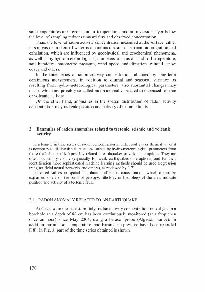
178

soil temperatures are lower than air temperatures and an inversion layer below the level of sampling reduces upward flux and observed concentration.

Thus, the level of radon activity concentration measured at the surface, either in soil gas or in thermal water is a combined result of emanation, migration and exhalation, which are influenced by geophysical and geochemical phenomena, as well as by hydro-meteorological parameters such as air and soil temperature, soil humidity, barometric pressure, wind speed and direction, rainfall, snow cover and others.

In the time series of radon activity concentration, obtained by long-term continuous measurement, in addition to diurnal and seasonal variation as resulting from hydro-meteorological parameters, also substantial changes may occur, which are possibly so called radon anomalies related to increased seismic or volcanic activity.

On the other hand, anomalies in the spatial distribution of radon activity concentration may indicate position and activity of tectonic faults.

2. Examples of radon anomalies related to tectonic, seismic and volcanic activity

In a long-term time series of radon concentration in either soil gas or thermal water it is necessary to distinguish fluctuations caused by hydro-meteorological parameters from those (called anomalies) possibly related to earthquakes or volcanic eruptions. They are often not simply visible (especially for weak earthquakes or eruptions) and for their identification more sophisticated machine learning methods should be used (regression trees, artificial neural networks and others), as reviewed by [17].

Increased values in spatial distribution of radon concentration, which cannot be explained solely on the basis of geology, lithology or hydrology of the area, indicate position and activity of a tectonic fault.

2.1. RADON ANOMALY RELATED TO AN EARTHQUAKE

At Cazzaso in north-eastern Italy, radon activity concentration in soil gas in a borehole at a depth of 80 cm has been continuously monitored (at a frequency once an hour) since May 2004, using a barasol probe (Algade, France). In addition, air and soil temperature, and barometric pressure have been recorded [18]. In Fig. 3, part of the time series obtained is shown.

179

Fig.3: Time series of hourly radon activity concentration in soil gas and soil temperature as well as earthquake magnitudes at Cazzaso, Italy from September 2004 to April 2005. Upper panel: full horizontal lines indicate the average seasonal radon concentration, dashed lines, 1 and dotted lines, 2 deviations from the seasonal

average; bottom panel: positive values of × are considered as radon anomalies. Radon anomalies were considered as: (i) deviations of CRn by more than 2

from the mean value and (ii) periods of equal signs (either + or –) of and . Both kinds of anomalies were observed three weeks prior to the

earthquake of ML=5.1, which occurred on November 24, 2004 at the Lake Garda, about 250 km away from our measurement point.

2.2. RADON ANOMALY RELATED TO VOLCANIC ACTIVITY

Radon activity concentration in outdoor air 50 cm above ground was continuously monitored (at a frequency once an hour) for a week, using an AlphaGuard device (Genitron, Germany), at two points on the flank of Mt. Etna in Sicily, one at the seashore in Stazzo and the other at Zafferana, about 5 km below the summit (3323 m) in the east-south direction[19]. Fig. 4 shows time variation of radon concentration, air temperature and barometric pressure (left), and time gradients of radon concentration and barometric pressure

(right).

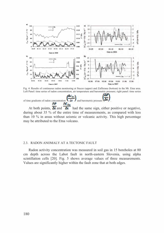
180

Fig. 4: Results of continuous radon monitoring at Stazzo (upper) and Zafferana (bottom) in the Mt. Etna area. Left Panel: time series of radon concentration, air temperature and barometric pressure; right panel: time series

of time gradients of radon concentration and barometric pressure .

At both points, and had the same sign, either positive or negative, during about 35 % of the entire time of measurements, as compared with less than 10 % in areas without seismic or volcanic activity. This high percentage may be attributed to the Etna volcano.

2.3. RADON ANOMALY AT A TECTONIC FAULT

Radon activity concentration was measured in soil gas in 15 boreholes at 80 cm depth across the Labot fault in north-eastern Slovenia, using alpha scintillation cells [20]. Fig. 5 shows average values of three measurements. Values are significantly higher within the fault zone that at both edges.

181

Fig. 5: Profile of radon activity concentration across the Labot fault in north-east Slovenia.

3. Conclusion

Radon anomalies in long-term time series of radon concentration in soil gas and thermal water have been found as precursors of earthquakes and volcanic eruptions. Radon anomalies in spatial distribution of radon concentration have appeared as indicators of tectonic faults. For anomaly identification (especially in cases of low magnitudes), machine learning techniques have been proven as very efficient and reliable.

References:

1. Ulomov, V.I. and B.Z. Mavashev, On forerunners of strong tectonic earthquakes. Doklady Akademii Nauk SSSR, 1967(176): p. 319–322.

2. Wakita, H., et al., Radon anomaly - possible precursor of the 1978 Izu-Oshima-Kinkai earthquake. Science, 1980. 207(4433): p. 882–883.

3. Lomnitz, C., Fundamentals of Earthquake Prediction1994, New York: John Wiley & Sons. 4. King, C.Y., Anomalous radon emanation of San Andreas fault. Transactions-American

Geophysical Union, 1976. 57(12): p. 957–957. 5. Nazaroff, W.W., B.A. Moed, and R.G. Sextro, Soil as a source of indoor radon: generation,

migration and entry, in Radon and its Decay Products in Indoor Air, W.W. Nazaroff and A.V. Nero Jr, Editors. 1988, John Wiley & Sons: New York.

6. Ota, M. and H. Yamazawa, Forest floor CO2 flux estimated from soil CO2 and radon concentrations. Atmospheric Environment, 2010. 44(36): p. 4529–4535.

7. Iskandar, D., H. Yamazawa, and T. Iida, Quantification of the dependency of radon emanation power on soil temperature. Applied Radiation and Isotopes, 2004. 60(6): p. 971–973.

8. Tanner, A.B.,Radon migration in the ground: a review, inNatural Radiation Environment, J.A.S. Adams and W.M. Lowder, Editors. 1964, University of Chicago Press: Chicago.

Fleischer, R.L., Dislocation model for radon response to distant earthquakes. Geophysical Research Letters, 1981. 8(5): p. 477–480.

10. Etiope, G. and G. Martinelli, Migration of carrier and trace gases in the geosphere: an overview. Physics of the Earth and Planetary Interiors, 2002. 129(3–4): p. 185–204.

182

11. Kristiansson, K. and L. Malmqvist, Evidence for nondiffusive transport of 22286Rn in the ground and a new physical model for the transport. Geophysics, 1982. 47(10): p. 1444–1452.

12. Vàrhegyi, A., et al., Experimental study of radon transport in water as test for a transportation microbubble model. Journal of Applied Geophysics, 1992. 29(1): p. 37–46.

13. Clements, W.E. and M.H. Wilkening, Atmospheric-pressure effects on Rn-222 transport across earth-air interface. Journal of Geophysical Research, 1974. 79(33): p. 5025–5029.

14. Chen, C., D.M. Thomas, and R.E. Green, Modeling of radon transport in unsaturated soil. Journal of Geophysical Research-Solid Earth, 1995. 100(B8): p. 15517–15525.

15. Klusman, R.W. and J.D. Webster, Preliminary analysis of meteorological and seasonal influences on crustal gas emission relevant to earthquake prediction. Bulletin of the Seismological Society of America, 1981. 71(1): p. 211–222.

16. Klusman, R.W. and J.A. Jaacks, Environmental influences upon mercury, radon and helium concentrations in soil gases at a site near Denver, Colorado. Journal of Geochemical Exploration, 1987. 27(3): p. 259–280.

17. Gregori , A., et al., Radon as earthquake precursor - methods for detecting anomalies, in Earthquake Research and Analysis, S. D'Amico, Editor 2011, Intech, in press.

18. Vaupoti , J., et al., A radon anomaly in soil gas at Cazzaso, NE Italy, as a precursor of an ML=5.1 earthquake. Nukleonika, 2010. 55: p. 507–511.

19. Vaupoti , J., P. Žvab, and S. Giammanco, Radon in outdoor air in the Mt. Etna area, Italy. Nukleonika, 2010. 55: p. 573–577.

20. Ho evar, M., Spatial distribution of radon in soil at the Labot fault. Graduation thesis (supervised by J. Vaupoti ), Faculty of Natural Sciences and Engineering, University of Ljubljana, 2005.

183

ANTARCTICA AS THE UNIQUE NATURAL LABORATORY FOR

DETERMINATION OF MAIN REASONS OF EARTH’S GLOBAL

CHANGES.

VALERY LYTVYNOV Head of National Antarctic scientific Centre Kiev, Ukraine uac@uac.gov.ua

Abstract. The role of Antarctic research for understanding both planetary regularities of the nature and reasons of the observed Earth’s global changes is shown in this paper. Main steps of a newly independent state Ukraine in Antarctica and some results of 15-years domestic research at the Antarctic Akademik Vernadsky station which is one of the important multidisciplinary observation points for all geospheres in the sub polar region are reported. Basic scientific areas of the new State Special-Purpose Research Program in Antarctica for 2011-2020 are presented; a special attention is paid to intermediate results in the sphere of geologic – geophysical research in the South Polar Region. The membership and Ukraine potentialities for participation in BlackSeaHazNet project are shown; it is suggested also to use the Ukrainian experience in: 1) fulfilment of joint works on monitoring of geodynamic shifts of Earth surface and large-block anthropogenic objects in quaky regions by the method of satellite radar interferometry; 2) creation of marine geoid topography in coastal zones by satellite altimetry data and provision of regular monitoring of sea surface topography changes, connected both with hydrodynamic processes of aqueous medium (sea currents, tsunami) and geodynamic shifts of seabed, in accordance with satellite reference trajectories; 3) creation by EGM 2008 and EGM96 geoid modern models of lithosphere deep structure tomographic models at different horizons for the purpose of possible earthquake sources decoding by the gravitation tomography method; 4) providing availability of Ukrainian Sich-2 satellite data for solution of wide range of meteorological (cloudiness, vortex-type flows at the sea surface), ecological and environmental issues on testing areas in different regions. Collaboration within indicated areas will favour further search of ways of practical use of BlackSeaHazNet project results.

184

At present the world scientific community has come to a common understanding that no scientific problem of global concern can be resolved without understanding the phenomena and processes on such a large space, like Antarctica, which takes about 10% of the Earth's surface. Climate change and associated risks including the increase in the number of natural disasters, difficult to predict - here are the priority issues that very well could be solved by comprehensive studies exactly in South Polar region of the Earth. Because you know that Antarctica, like a Gulf Stream in the Northern hemisphere, is an important climate forming factor for the entire planet. All basic natural areas of the Earth are studied in Antarctica – from the Earth’s Core and sub glacial lakes (suspended models of prehistoric ecosystems) to the upper atmosphere and magnetosphere. Here are the best conditions for the exercise of uninterrupted research both short-term geomagnetic phenomena (auroras, radio wave connection disturbance) and long-term phenomena connected with ozone layer depletion, stratospheric winds and space weather. The scope of research allows getting a holistic understanding of planetary patterns (Gozhik et al., 2009).

Particularly important is the fact that Antarctica is far from sources of pollution. Minimum sound noise, vibrations and electromagnetic disturbances caused by human activities make the region especially important to study the seismic activity, as those processes hidden in other regions by anthropogenic noise are available for monitoring in Antarctica. So, by studying the energy transfer in the lithosphere-atmosphere-ionosphere waveguide it is possible to single out precursor effects of earthquakes in infrasonic, geomagnetic and electromagnetic data.

Ukrainian scientists working in Antarctica have made a significant contribution to the understanding of these processes. Even before the collapse of the Soviet Union, Ukrainian scientists and engineers took an active part in studies of Antarctica. Becoming an independent State, Ukraine in September 1992, had acceded to the Antarctic and a year later, on the basis of the National Academy of Sciences was established the first Ukrainian Antarctic Centre. Regular polar research of the sixth continent our country began in 1996,

1996 , after the United Kingdom handed over to Ukraine the

Faraday. The station received Akademik Vernadsky title in honour of the first President of the Academy of Sciences of Ukraine, author of the Earth’s noosphere teaching.

The station is located 10 kilometres west of the Antarctic Peninsula in the Argentine Islands archipelago. The modern station complex consists of 10 buildings of housing and laboratory-technical purpose and has a reliable system of life support. (Fig. 1).

185

Fig. 1 General view of Akademik Vernadsky station (photo from NASC archive)

Station is one of the few geophysical observatories on the continent which

may boast half a century old series of continuous measurements. And over time the number and quality of observations constantly grows. The measurements carried out at the station affect practically all environmental parameters that attract the leading Ukrainian scientific institutions with their enormous scientific potential. Therefore in the new State Special-Purpose Research Program in Antarctica for 2011-2020 a significant part is assigned to Earth sciences, particularly to earth shell geophysics. These areas are presented in NASC by leading instituted of the NAS of Ukraine: Institute of Geophysics, Institute of Geological Studies, Institute of Radio Astronomy, Hydrometeorological Research Institute, etc. (Gozhik et al., 2010).

Geological-geophysical studies are carried out both at Vernadsky station (seismological observations and a wide range of magnetic measurements) and on board the research vessels (bottom topography of the South ocean and shallow archipelagos, magnetic and gravimetric surveys) involving modern satellite data from Ukraine, European Space Agency, USA and Germany.

One of the interesting and topical challenges being solved at the Antarctic station using complex interdisciplinary approach is monitoring and natural hazards risk assessment in the Antarctic Peninsula area.

Being an overwintering station it is well equipped for ionosphere sounding research, meteorological and magnetic observations, studies of ozone layer and electromagnetic processes in the environment, as well as acoustic observations,

186

since an earthquake is considered to be the most high-energy phenomenon the response from which penetrates into all geophysical fields. Therefore for the complex analysis and assessment of seismic activity tidal, seismic, infrasonic, meteorological, electromagnetic, and geomagnetic and radon data are used. So, on the basis of geomagnetic measurements made close to Galindez Island there was discovered a magnetic anomaly being changed with a course of time that reflects accumulation of the Earth’s crust deformation in the region. Five-year measurements showed the overall correlation of changes of magnetic field and integral amount of radon emanated from the Earth’s crust on geomagnetic measurements sites. In turn, model calculations of the Earth’s crust deformation and their comparison with radon and magnetic data have shown that the integral radon emanation is in direct proportion to the conventional strain.

On the basis of such measurements and calculations, a conclusion concerning long-term earthquake forecasts can be made – permanent monitoring of integral radon emanation may allow to reveal places of deformation storage and consequently to identify possible epicentres of future earthquakes close to which equipment for medium-term and short-term forecasts should be installed (Fig.2).

Fig. 2. Change of radon data distribution law: the earthquake in the Scotia Sea, Antarctic Peninsula (left) and Vrancea area (right) is marked by arrow signs.

Processing of measuring results and their comparison with seismic, acoustic

and meteorological data have shown that radon emanation can “feel” even remote earthquakes which regularly take place in the Scotia Sea (at a distance of about 1000 – 1500 km from the station). However, preparation for an earthquake is revealed not in the amplitude anomaly (as it is usually supposed) but in the statistical anomaly, i.e. in the change of statistical distribution of detected radon – Poisson distribution that is usual for aseismic regions changes for the Neumann type distribution (Liashchuk, & Pavlovich, 2011). As it is shown the

187

received and tested methods may be successfully used in other regions of the planet, particularly in the Vrancea area (Fig.3).

Fig. 3. Application results of radon concentration data processing by wavelet-method: left – earthquakes peaks

>4 observed in the Vrancea area, 2005; right – radon concentration data at Vernadsky station, 2010; strong earthquakes ( >=6) 550 away are marked by arrow signs (left arrow) and the forecasted earthquake 830 km away (right arrow).

Concepts of Professor Vazira Martazinova are also of great interest. She has

found a connection between atmospheric phenomena (strong fall of temperature) and earthquakes (Martazinova, 2011). However, for in-depth study of seismic activity the use of satellite data is needed. Taking into consideration the subject matter of the meeting, I would like to pay more attention to methods of remote sensing and modelling of the Earth lithosphere deep structure.

Remote methods of sensed observations play an active part for studying of remote and hard-to-reach areas of Antarctica. Already over the years the Institute of geological sciences with the support of NASC receives in the framework of the European space agency grant the information from EPC-1 and EPC-2 satellites through high-precision radio altimetry channels to determine sea surface (or geoid) topography conditional on terrestrial gravitational field, as well as radar photos for interferometer processing, determination of the detailed topography and vertical and horizontal shifts of the Earth surface. (Fig.4).

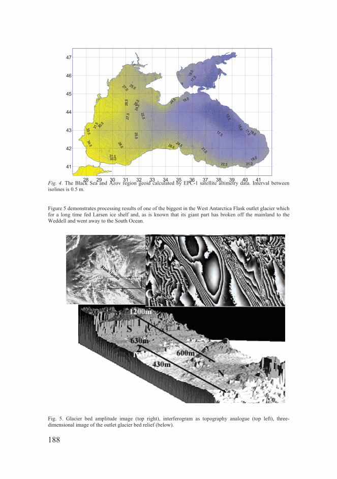
188

Fig. 4. The Black Sea and Azov region geoid calculated by EPC-1 satellite altimetry data. Interval between isolines is 0.5 m.

Figure 5 demonstrates processing results of one of the biggest in the West Antarctica Flask outlet glacier which for a long time fed Larsen ice shelf and, as is known that its giant part has broken off the mainland to the Weddell and went away to the South Ocean.

Fig. 5. Glacier bed amplitude image (top right), interferogram as topography analogue (top left), three-dimensional image of the outlet glacier bed relief (below).

28 29 30 31 32 33 34 35 36 37 38 39 40 41

41

42

43

44

45

46

47

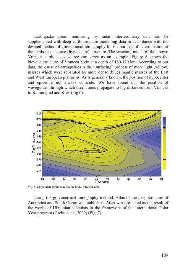
189

Earthquake areas monitoring by radar interferometry data can be

supplemented with deep earth structure modelling data in accordance with the devised method of gravitational tomography for the purpose of determination of the earthquake source (hypocentre) structure. The structure model of the known Vrancea earthquakes source can serve as an example. Figure 6 shows the bicyclic structure of Vrancea body at a depth of 160-170 km. According to our data, the cause of earthquakes is the “surfacing” process of more light (yellow) masses which were separated by more dense (blue) mantle masses of the East and West European platforms. As is generally known, the position of hypocenter and epicentre not always coincide. We have found out the position of waveguides through which oscillations propagate to big distances form Vrancea to Kaliningrad and Kiev (Fig.6).

Fig. 6. Carpathian earthquake source body, Vrancea area.

Using the gravimetrical tomography method, Atlas of the deep structure of

Antarctica and South Ocean was published. Atlas was presented as the result of the works of Ukrainian scientists in the framework of the International Polar Year program (Greku et al., 2009) (Fig. 7).

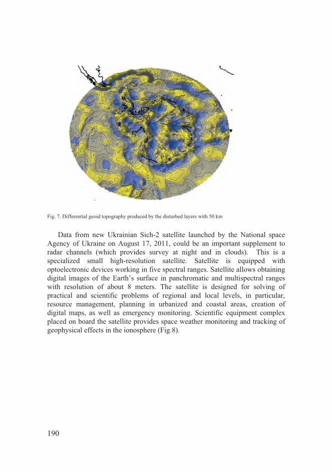
190

Fig. 7. Differential geoid topography produced by the disturbed layers with 50 km

Data from new Ukrainian Sich-2 satellite launched by the National space

Agency of Ukraine on August 17, 2011, could be an important supplement to radar channels (which provides survey at night and in clouds). This is a specialized small high-resolution satellite. Satellite is equipped with optoelectronic devices working in five spectral ranges. Satellite allows obtaining digital images of the Earth’s surface in panchromatic and multispectral ranges with resolution of about 8 meters. The satellite is designed for solving of practical and scientific problems of regional and local levels, in particular, resource management, planning in urbanized and coastal areas, creation of digital maps, as well as emergency monitoring. Scientific equipment complex placed on board the satellite provides space weather monitoring and tracking of geophysical effects in the ionosphere (Fig.8).

191

Fig. 8. Sich-2 spacecraft: top and bottom view.

Thus, the main findings of the report are the following. First, Ukrainian

Antarctic Akademik Vernadsky station is the important area of geophysical observations. As a result a unique technical complex opened for any measurement equipment and new methods of investigations was created at the station. Usage of Usage of different data creates the necessary prerequisites for an interdisciplinary approach to scientific problems solving connected with studies of climate, solar activity and ionosphere, stratospheric ozone dynamics, space weather, tectonics, seismicity, ice behaviours etc.

192

Second, we offer to use our experience and scientific potential of NASC and Ukrainian institutes in the following spheres:

4. Execution of joint works on monitoring of geodynamic shifts of the Earth surface and large-block anthropogenic objects in quaky areas by the method of satellite radar interferometry;

5. Creation of sea geoid topography in coastal zone by satellite altimetry data and also provision with regular monitoring of sea surface topography changes received using reference trajectories of satellites connected both with aqueous medium hydrodynamic (currents, tsunami) and geodynamic shifts of the seabed;

6. Using geoid EGM 2008 and EGM 96 geoid modern models creation of deep lithosphere structure tomographic models of at different horizons for the purpose of decoding of possible earthquake sources by gravitation tomography method;

7. Guarantee the possibility of usage of Ukrainian Sich-2 satellite data for solving of a wide range of meteorological (cloudiness, vortex formations at a sea surface), ecological and environmental issues at testing areas in different regions.

The basic aim of BlackSeaHazNet project is to set up a research team. After two years it is necessary to clarify its membership and, if necessary, to include new scientists with wide experience since the basic aim of the team will be elaboration of appropriate preliminary specifications and a hardware-software complex of the natural cataclysms early control in the Black Sea area. Availability of not only new knowledge but of such powerful tools will undoubtedly favour the further search of means of our research results practical use.

Reference

Gozhik P.F., Gurzhiy A.M., Lytvynov V.A., 2009. Scientific research in the Antarctic Treaty

System. Ukrainian Antarctic Journal, 8: 32-38. Gozhik P.F., Lytvynov V.A., Malanchuk V.M., 2010. Ukraine scientific activity in Antarctica for

the decade Ukrainian Antarctic Journal, 9: 7-15. Greku R.Kh. et al., 2009. Atlas of the Antarctic deep structure with the Gravimetric Tomography.

– Kiev. – 69 p. Liashchuk, J., Pavlovich, V., 2011. Goephysical anomalies before earthquakes in the Antarctic

Peninsuka region. BlackSeaHazNet Methodological-Coordination Workshop, 2-5 May 2011, Ohrid, Macedonia, Volume 1: 205-212.

Martazinova, V., 2011. On possible influence of earthquake preparation on weather and synoptic processes. BlackSeaHazNet Methodological-Coordination Workshop, 2-5 May 2011, Ohrid, Macedonia, Volume 1: 103-124.

193

GEOMAGNETIC-QUAKE AS EARTHQUAKES PRECURSOR: DATA

OF SOME INTERMAGNET OBSERVATORIES DURING 01/01 -

08/01/2011

V. BAKHMUTOV1, S. CHT. MAVRODIEV2, *T. MOZGOVA1, G. MELNYK1, O. MAKSIMENKO1, Z. JORDANOVA2

1 S.I.Subbotin Institute of Geophysics of National Academy of Sciences of Ukraine, 2 Institute for Nuclear Research and Nuclear Energy, Bulgarian Academy of Sciences

Abstract. The preliminary results in our research about possibilities of application of methods, which can distinguish Geomagnetic- Quake as an Earthquakes precursor in Vrancea and Japan regions are presented according to data of Ukrainian KIV observatory and according to KAK, MMB, KNY INTERMAGNET observatories data. It has been noticed that the quantity and reliability of determination of Geomagnetic signal, depending on the level of geomagnetic activity, frequency and energy of earthquakes, requires further exploration.

4. Introduction

The solution of the problem of Earthquakes prognosis in the terms of the project “BlackSeaHaz Net” is based on the correlation between observed Geomagnetic-Quake G-Q and coming min\max tidal gravitational potential (tidal wave) (Mavrodiev et al., 2006). It is supposed to use magnetic field components observations in extended international network stations INTERMAGNET, situated in distance <900 km from seismic active zones.

Nowadays on the territory of Ukraine the magnetic field observations are carried out by three magnetic observatories: Kiev- KIV, (50.7ºN, 30.9ºE ), Lvov – LVV(49.9N, 23.75E), Odessa – ODE (46.6N, 30.9E). In addition Ukraine has also the observatory on Argentinian Islands- AIA(65.25ºN, 295.75ºE), situated in Antarctic peninsula (West Antarctica), and a number of seismic stations, where the magnetic field observations are carry out. Three of these observatories (LVV, KIV and AIA) work in the NTERMAGNET (fig. 1). The data of observatory KIV have been used for finding of morphological features in the structure of geomagnetic variations in relation to earthquakes in Vrancea

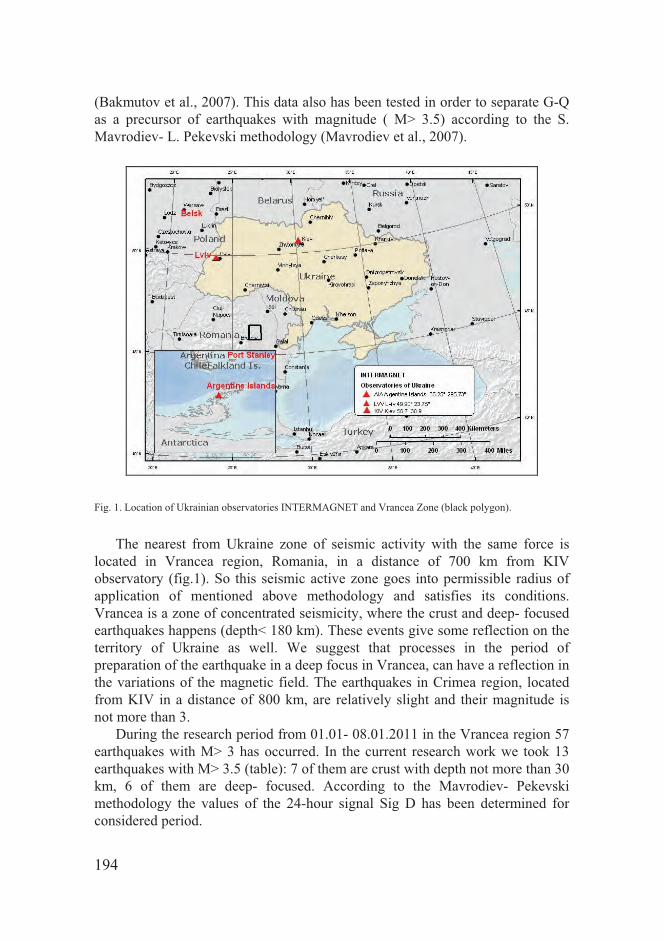
194

(Bakmutov et al., 2007). This data also has been tested in order to separate G-Q as a precursor of earthquakes with magnitude ( M> 3.5) according to the S. Mavrodiev- L. Pekevski methodology (Mavrodiev et al., 2007).

Fig. 1. Location of Ukrainian observatories INTERMAGNET and Vrancea Zone (black polygon).

The nearest from Ukraine zone of seismic activity with the same force is

located in Vrancea region, Romania, in a distance of 700 km from KIV observatory (fig.1). So this seismic active zone goes into permissible radius of application of mentioned above methodology and satisfies its conditions. Vrancea is a zone of concentrated seismicity, where the crust and deep- focused earthquakes happens (depth< 180 km). These events give some reflection on the territory of Ukraine as well. We suggest that processes in the period of preparation of the earthquake in a deep focus in Vrancea, can have a reflection in the variations of the magnetic field. The earthquakes in Crimea region, located from KIV in a distance of 800 km, are relatively slight and their magnitude is not more than 3.

During the research period from 01.01- 08.01.2011 in the Vrancea region 57 earthquakes with M> 3 has occurred. In the current research work we took 13 earthquakes with M> 3.5 (table): 7 of them are crust with depth not more than 30 km, 6 of them are deep- focused. According to the Mavrodiev- Pekevski methodology the values of the 24-hour signal Sig D has been determined for considered period.

195

Table. Earthquakes in Vrancea region during 7 months of 2011.

Data and time coordinates Deep

h, km

Magni-tude

Tide extreme, 0-min, 1-max

Time difference, day

Distance, 102 km

, º , º

1/14/2011 5:03 48.14 33.29 30 3.9 0 2.71 3.57 1/26/2011 23:57 45.09 27.57 22 3.5 0 1.5 6.56 2/04/2011 23:25 45.73 26.76 110 4 1 4.48 6.11 2/05/2011 14:28 45.56 26.55 120 3.6 0 -3.9 6.35 2/19/2011 20:00 45.8 26.77 73 3.8 1 3.33 6.04 3/14/2011 9:13 44.93 22.42 4 3.5 0 2.88 8.7 3/25/2011 15:12 45.61 22.86 2 3.8 0 -2.87 7.9 4/17/2011 11:41 45.62 26.42 120 4 1 -1.01 6.34 5/01/2011 2:24 45.6 26.58 150 4.7 1 -3.4 6.3 5/04/2011 10:43 45.07 29.85 10 3.8 1 -0.05 6.27 6/14/2011 10:48 45.68 26.56 146 4 1 -1.05 6.23 6/24/2011 13:08 47.46 25.86 2 4.4 0 1.05 4.84 7/12/2011 13:17 49.95 18.5 5 3.5 1 -0.95 8.41 7/14/2011 4:17 49.91 18.47 5 3.5 1 0.68 8.44

The geomagnetic precursor G-Q has been separated before every earthquakes

with M> 3.5 (fig. 2ab). In connection between G-Q and the next maximum of tidal wave, the prognosis of earthquakes has been made with certain level of accuracy, namely for minimum the average value is ±2.5 days, and±2 days for maximum.

Data of the monitoring of the observatory in Kiev is available on the website: http//stardust.inrne.bas.bg/mavrodi/.

196

a)

b)

Fig. 2. Daily geomagnetic (KIV observatory) and earthquakes monitoring for Jan-Mar (a) and Apr-Jul (b), 2011.

Geomagnetic field variations registered in the observatory, are caused by

different sources: external (magnetospheric and ionospheric current systems) and internal (induced by currents inside Earths). For this period the interplanetary magnetic field (IMF) in the solar wind has mainly two- sectored

197

structure. From 27 earthquakes with M>3, observed in Vrancea region during the positive IMF, crust earthquakes happen twice more often than deep- focused. In the negative IMF sector the quantities of crust and deep- focused earthquakes are equal. After coming to the Earth of high- speed flows of the Sun plasma (550 km\s) on 7th April the geomagnetic field disturbances have developed. They have been attended by jump of proton density and solar wind pressure 2HPa, and increases of the azimuthal electric field value to 4 mB\m and magnetic field B= 17 nT.

Geomagnetic storm with intensity Dst =-57nT (disturbance storm time index) and Dst=-40nT have been observed on 12th and 20th April. All geomagnetic storms have attended by high values of southern component of the IMF (Bz=-(8-13)nT).

Magnetic field was higher on April than on January: there was 5 Magnetic storms and intensive substorms (AL=-700-1000nT) on April and just 1 magnetic storm on January.

12 earthquakes events (4 of them were on the depth of 2 km) on April happened during the days with index Ap<8, including also a deep- focused earthquake with depth of 120 km, M= 4 in Vrancea, 17th Apr, Ap=3.

We consider that the variations, caused by external sources can influence on the separated geomagnetic signal (Daily Signal). The comparison of daily signal and standard planetary Am index of the geomagnetic activity for the period from 01.01 to 01.08.2011 has shown that daily signal and separated precursor G-Q in Vrancea region with M>3.5 in radius of 900 km from the observatory of Kiev, depend on total geomagnetic activity. Therefore, for greater reliability of G-Q separation is necessary to take into account the current level of geomagnetic activity, which is a subject of further research.

Data of observatory in Kiev are available for the analysis and processing in daily files of 1- second XYZ components data and 1- minute data in format INTERMAGNET JAGA 2002 form January 2011. This has helped to make a comparison of G-Q separated in average minute and second value data for both periods, where in Vrancea zone the earthquakes with M> 3.5 has been observed ( fig.3ab). According to preliminary data, before Earthquakes in Vrancea zone, G-Q is separated reliably by1-second and 1-minute data of KIV observatory.

198

a)

b)

Fig. 3. Comparison of geomagnetic precursor G-Q before coming earthquakes with M> 3.5 by1-second and 1-minute data of KIV observatory, observed in the periods 04- 20.01.2011 and 10.04- 05.05.2011.

This data give much more possibilities for application of mentioned above

methodology. In particular, the region of Japan has been considered in connection with the catasrophic Earthquake happened on 11.03.2011. On the territory of Japan 3 INTERMAGNET observatories: Memambetcu MMB, Kakkioka KAK and Kanoya KNY are located (fig.4). According to their data, the geomagnetic signal values by Mavrodiev-Pekevski methodology have been calculated (fig. 5). The increase of the Geomagnetic signal level 3 days before the incoming earthquake on 11.03.2011 has been observed.

There is an increase of earthquakes energy in the period from 9.03 to 16.04.2011. After 16.04 this energy becomes lower than before 9.03, but the frequency of earthquakes becomes higher. Probably this fact can explain just insignificant decrease of the signal after 16.04 (around 0.5nT). The total level of geomagnetic activity increases starting from 16.04. That also can influence on the geomagnetic signal level.

199

Fig.4. Japanese observatories INTERMAGNET and location of the main quantity of

Earthquakes in the period from 01.01 to 08.01.2011 (black polygon)

200

b)

c)

Fig. 5 Data of the monitoring of geomagnetic field and earthquakes for Japan in the period from Jan to Jul, 2011 ( observatories MMB a), KAK b), KNY c)).

Thereby the preliminary data for the research of geomagnetic quake as a

pecursor for earthquakes has shown that:

201

• in Vrancea region (according to data of KIV obsrevatory ) geomagnetic quake can be distinguished by 1- second and 1-minute data. The value of geomagnetic precursor G-Q of the earthquakes with M> 3.5 according to preliminary data is not more than 7%.

• according to Japan observatories data the increase of the signal has been noticed before incoming Earthqake on 11.03.2011. According the preliminary data the frequency of earthquakes influences on the level of the geomagnetic signal.

• the value and reliability of determination of the G-Q depends on the level of geomagnetic activity, frequency and energy of earthquakes, which require further studies.

References

Bakhmutov V., Sedova F., Mozgovaya T. Morphological Features in the Structure of Geomagnetic Variations in Relation to Earthquakes in Vrancea\\ Publs. Inst. Geophys. Pol.Acad.Sc. C-99 (398). – 2007. –C.366-373.

Mavrodiev S. Cht. On the reliability of the geomagnetic quake as a short time earthquake’s precursor for the Sofia region // 2004, http://www.nat-hazards-earth-syst-sci.net/4/433/2004/nhess-4-433-2004.pdf

Mavrodiev S. Cht., Bakhmutov V., Mozgovaya T. The Kiev Intermagnet data and some preliminary results in the framework of INRNE, BAS gemagnetic and earthquake monitoring // “Global Changes, Environment, Sustainable Development of the Society and High Mountain Observatories Network”, BEOBOL Conference, 21-25 March 2007, Gyulechitsa, Bulgaria. – Observatoire de Mountagne, de Moussala OM2, 12, 2007, Sofia. Institut de recherché nucleaire et d’energie nucleaire, Academie bulgare des Sciences, BEOBOL, FP6 Progect, INCO-CT-2005-016663, P.238-243

Mavrodiev S. Cht., Pekevski L., Jimseladze T. Geomagnetic-Quake as Imminent Reliable Earthquake’s Precursor: Starting point for future complex regional NETWORK // 2006, http://theo.inrne.bas.bg/~mavrodi/

*Contact person: Tamara Mozgova, S.I.Subbotin Institute of Geophysics of NASU, Palladin av., 32, Kyiv, Ukraine 03680, e-mail: mozgowa@igph.kiev.ua

202

COSMO-PHYSICAL APPROACH TO EARTHQUAKE FORECASTING

1N.G. KHAZARADZE, G.K. VANISHVILI, 1T. S BAKRADZE, 2L.B. KORDZADZE, M.3ELIZBARASHVILI, E. BAZERASHVILI

1. Cosmo-Physical Complex for Registration of Cosmic Rays Variations, The Sector of Solar-Terrestrial Physics, Michael Nodia Institute of Geophysics, Ivane Javakhishvili Tbilisi State University. 2. Department of Physics, Akaki Tsereteli Kutaisi State University 3. Faculty of Physics, Ivane Javakhishvili Tbilisi State University.

e-mail: nodarkhaz@yahoo.co.uk

Abstract. The process of crossing of the neutral layer of the Interplanetary Magnetic Field (IMF) is presented as the most geo-effective for stimulation of the strong destructive earthquakes, in comparison with all nontraditional cosmo-physical phenomena which strictly or indirectly may be tied with it. During the Solar flare when the Solar plasma flux or so called Solar Wind is blowing on our planet - the magnetosphere of the Earth undergoes the deformation of its shape... The quota of force lines of the magnetic field “frozen” in the substance of plasma are shifted from day side to night-side. As far as our planet represents the body moving around its axis of rotation, and the quota of its’ mass is shifted in direction, perpendicular to the axis of rotation, c consequently its Moment of Inertia “ I ” undergoes alteration, which in its turn is undoubtedly leads to corresponding alteration of angular velocity rotation “ ω “, according to the fundamental law of conservation of momentum of inertia L=[I * ω ]= const. Repeated reports (announcements) of various authors about spasmodic (uneven) alteration of Terrestrial rotation after the strong flashes on the Sun [1] . . . and finally our preliminary investigations [2] . . . may be served as a confirmation of all stated above. . . More than 500 earthquakes, with magnitude M≥6 have been registered for more than 35 years period, were analyzed. It was found that more then 70 % of the strong destructive earthquakes takes place when the Earth is approaching and crossing the neutral layer of IMF, and it is in a good correlation with 11-years Solar Activity cycle.

Keywords: Neutral Layer of the Interplanetary Magnetic Field (IMF), earthquake.

203

1. Cosmo-Physical Approach to Earthquake Forecasting

We would like to make a short, and as it seems to us, sensational statement from a small group of the Sector of Solar-Terrestrial Physics, at Institute of Geophysics.Just almost during 10 years our group is occupied by questions of nontraditional forecasting of the strong destructive earthquakes with taking into account the Cosmic Rays.The nontandard cosmo-physical method for forecasting of the strong destructive earthquakes , which is based on the Law of Conservation of Momentum of the Quantity of Motion of the Earth, according to our suggestion, was yielded with the sensational results! More than 500 earthquakes with magnitude M 6, for the period of 35 years, was analyzed. It was found that above mentioned earthquakes were occurred at the moment of crossing of Neutral Layers of the Interplanetary Magnetic Field (IMF) by the Earth, and are in good correlation with the Solar Flares.The number of coincidence of earthquakes times with the moments of Earth's passage through the Neutral Layers of the IMF is more than 75% from total number of earthquakes, have been occurred and have been reviewed. Such a high rate of percent of correlation can not be sporadic, or accidental or occasional. But we have bound it with above mentioned fundamental Law of Nature, theoretical essence and practical effectiveness of which is still the subject of further elaboration. . .Diverting our attention from rapid, quick, sudden inferences or conclusions, for the given stage of development, this method gives us the possibility to forecast the earthquake dates for week ahead and magnitudes with M 6. The determination of the earthquake coordinates is the mission of the Regional Seismological Services, which will receive the Regular International Messages on forthcoming Seismological Hazards. Thus, the efforts of the Cosmo-Physical Method, suggested by us, and Traditional Instrumental Seismology are unified, creating inseparable united whole, which must lead us to the desired success.

2. Conclusion.

If we shall follow by positions which often takes place in science in general, when investigations in different directions are suddenly intersected in the “critical dots”, and this intersection is occurred to be completely effective and fruitful, then we can affirm confidently, that our case, which is unifying the efforts of instrumental seismology and cosmo-physical method may be yielded in desired result.

204

References.

1. Shatashvili L.Kh., Sikharulidze D.I., Khazaradze N.G., Tutberidze N.G. Anomalous diurnal variations of neutron and rigid component of cosmic rays in crossing the neutral layer of the IMF by the Earth. Izv. RAN, Physical Ser., 1999, v 63, No 8, pp. 1645-1648.

2. Khazaradze N.G., et al Anomalous Solar-Diurnal variations in cosmic rays related to crossing of the IMF Sector Boundaries by the Earth and the problem of Earthquakes. Geomagnetism and Aeronomy, vol 4., No 3, pp.395-398.

3. Asatryan G.I., Asatryan Gr. A. et al Izvest Ran. Physical Ser., v 55, No 10, pp 1979-1982. 4. Dorman L.I., Galactical Cosmic Rays Variations. Izdat. AN SSSR, Moscow, 1975.

205

Part III. Training “Geomagnetic precursors”

STUDY OF GEOMAGNETIC VARIATIONS IN GEORGIA AND

ESTABLISHMENT OF ANOMALY NATURE OF EARTHQUAKE

PRECURSORS

TAMAR JIMSHELADZE1, GEORGE I. MELIKADZE1, GIORGI KIKUASHVILI, S. MAVRODIEV2, L. PEKEVSKI3 , MARINE CHKHITUNIDZE 1. M. Nodia Institute of Geophysics, Iv. Javakhishvili Tbilisi State University 2. Institute for Nuclear Research and Nuclear Energy, Bulgarian Academy of Sciences, Sofia, Bulgaria 3. Seismological Observatory, Faculty of Natural Sciences and Mathematics, Skopje, R. Macedonia

Abstract

Before strong earthquake magnetic precursors denoted by many authors, but must to say, that more of them don’t satisfy stern criterions. There are many examples of geomagnetic anomaly in Georgia too: a few weeks before earthquakes in Spitak, anomaly grows of low frequency geomagnetic pulsation amplitudes were fixed in Geophysics Laboratory of Dusheti. The, “When, where and how” earthquake prediction problem is not solved but is an actual problem for a long time. From 1989 researches on possible connection between geomagnetic variations and incoming earthquake started in INRNE. (Mavrodiev S. Cht., Thanassoulas C., Possible correlation between electromagnetic earth fields and future earthquake, INRNE-Bas, Seminar proceeding, July 23-27, 2001, Sofia, Bulgaria, ISBN 954-9820-05-X,2001). From February 2006 Ukraina was included in INRNE, BAS geomagnetic and Earthquake monitoring. From January 2009 Georgia with its Geomagnetic observatory of Dusheti was also included in INRNE, BAS. For estimation of the geomagnetic variations as a reliable precursor the specific time analysis was discovered for digital definition of Geomagnetic Quake and proposed a way for interval defined from the extremum of local tide variations [ S. Cht. Mavrodiev, 2001]. Georgian Geomagnetic stations can input important information for space dependences of precursor intensity as part of complex regional NETWORK of PrEqTiPlaMagInt

206

collaboration (Prediction Earthquake Time Place Magnitude Intensity). We introduce the primary work-up results of data received from the Dusheti Magnetic Observatory which was worked up for investigation of earthquake prediction on the basis of geomagnetic variations. Keywords: precursor; geomagnetic quake; earthquake; tide difference; tidal extreme; density of earthquake radiated energy.

1. Introduction Georgia is a part of the far-extending seismically active region, which includes the whole Caucasus, Northern parts of Turkey, and Iran. These territories witnessed several intense destructive earthquakes. Thus carrying out possible short-term prognosis of earthquakes is very important for the country. Before strong earthquake magnetic precursors denoted by many authors, but must to say, that more of them do not satisfy stern criterions. There are many examples of geomagnetic anomaly in Georgia too: a few weeks before earthquakes in Spitak, anomaly growth of low frequency geomagnetic pulsation amplitudes was fixed in Geophysics Laboratory of Dusheti. The problem of ,,when, where and how” earthquake prediction cannot be solved only on the basis of seismic and geodetic data(Aki,1995; Pakiser and Shedlock,1995; et al., 1997; Ludwin,2001). The possible tidal triggering of earthquakes has been investigated for a long period of time. Including of additional information in the precursors monitoring, such as the analysis of the electromagnetic field variations under, on and above the Earth surface, can contribute towards defining a reliable earthquake precursor and estimating the most probable time of a forthcoming earthquake. Simultaneous analysis of more accurate space and time measuring sets for the earth crust condition parameters, including the monitoring data of the electromagnetic field under and over the Earth surface, as well as the temperature distribution and other possible precursors, would be the basis of nonlinear inverse problem methods. it could be promising for studying and solving the ,,when, where and how” earthquake prediction problem. Some progress for establishing the geomagnetic filed variations as regional earthquakes’ precursors was presented in several papers (Mavrodiev, Thanassoulas, 2001; mavrodiev, Pekevski, Jimsheladze, 2008). The approach is based on the understanding that earthquake processes have a complex origin. Without creating of adequate physical model of the Earth existence, the gravitational and electromagnetic interactions, which ensure the stability of the Sun system and its planets for a long time, the earthquake prediction problem cannot be solved in reliable way. The earthquake part of the model have to be repeated in the infinity way “theory- experiment- theory” using nonlinear

207

inverse problem methods looking for the correlations between fields in dynamically changed space and time scales. Of course, every approximate model (see for example Varotsos, 1984, a, b, Varotsos et al, 2006; Thanassoulas, 1991; Thanassoulas et al., 2001a, b; Eftaxias at all, 2006, Duma, 2006) which has some experimental evidence has to be included in the analysis. The adequate physical understanding of the correlations between electromagnetic precursors, tidal extremums and incoming earthquake is connected with the progress of the adequate Earth’s magnetism theory as well as with quantum mechanical understanding of the processes in the earthquake source volume before and during an earthquake.

The achievement of the Earth’s surface tidal potential modeling, which includes the ocean and atmosphere tidal influences, is an essential part of the research. In this sense the comparison of the Earth tides analysis programs on Venedikov et al.., 2003; Milbert,2011) is very useful.

The role of geomagnetic variations as precursor can be explained by the hypothesis that during the time before the earthquakes, with the strain, deformation or displacement changes in the crust there arise in some interval of density changing the chemical phase shift which leads to an electrical charge shift. The preliminary Fourier analysis of geomagnetic field gives the time period of alteration in minute scale. Such specific geomagnetic variation we call geomagnetic quake. The last years results from laboratory modelling of earthquake processes in increasing stress condition at least qualitatively support the quantum mechanic phase shift explanation for mechanism generating the electromagnetic effects before earthquake and others electromagnetic phenomena in the time of earthquake (Freund et al, 2002; St-Laurent et al, 2006, Vallianatos et all, 2003, 2006)

The future epicentre coordinates have to be estimated from at least 3 points of measuring the geomagnetic vector, using the inverse problem methods, applied for the estimation the coordinates of the volume, where the phase shift arrived in the framework of its time window. For example the first work hypothesis can be that the main part of geomagnetic quake is generated from the vertical Earth Surface- Ionosphere electrical current. See also the results of papers (Vallianatos, Tzanis, 2003 ; Duma, Ruzhin, 2003, Duma, 2006 ) and citations there.

In the case of incoming big earthquake (magnitude > 5 - 6) the changes of vertical electropotential distribution, the Earth’s temperature, the infrared Earth’s radiation, the behaviour of debit, chemistry and radioactivity of water sources, the dynamics and temperature of under waters, the atmosphere conditions (earthquakes clouds, ionosphere radioemitions, and etc.), the charge density of the Earth radiation belt, have to be dramatically changed near the epicentre area.

The achievements of tidal potential modeling of the Earth’s surface, including ocean and atmosphere tidal influences, multi- component correlation analysis and nonlinear inverse problem methods in fluids dynamics and

208

electrodynamics are crucial for every single step of the constructing of the mathematical and physical models.

3. Method

In the paper (Mavrodiev,2004) the geomagnetic quake was defined as a jump of the day mean value of the signal function Sig:

(1) Here Hm is the standard deviation of geomagnetic field component Hh, and

Hm is the corresponding error, Hm is one-minute averaged value of geomagnetic vector projection Hi, M=1440 minutes per day, and N=60 are the samples per minute. The predicted earthquake is identified by the maximum of the function

proportional to the density of the earthquake radiated energy in the monitoring point. The analytical size of this function is:

SChtM = 10M / (D+Depth +Distance2), (2) Where the distances are in hundred km, fit parameter D = 40 km and M is

the earthquake magnitude Thus, if we have a jump of signal function Sig and its error Sig is such

that satisfies numerically the next condition: SigToday – SigYesterday > ( SigToday + SigYesterday) / 2, (3) In the next tidal extreme time the function SChtM will have a local

maximum value. The earthquake for which the function SChtM has a maximum can be interpreted as predicted earthquake.

The probability time window for the incoming earthquake or earthquakes is approximately ± 1 day for the tidal minimum and for the maximum- ± 2 days.

The analytical size of the function SChtM as well as one minute time period for calculating the unique signal for geomagnetic quake which is reliable earthquake precursor was established by Dubna inverse problem method (Dubna Papers).

,/ 1

MSigM

mHm

=

= σ ,/ 1

MSigM

mHm

=

= δσδ

,)(,1

2

=

−=Nt

mt

NHH

mHσ ,)(,1

2

=

−=Nt

mt

NHH

mHδδδσ

==

N

i NHH i

m1

,1=

=N

i NHH i

mδδ

209

In the case of vector geomagnetic monitoring, one has to calculate the minute standard deviation as a geodynamical sum of standard deviations of the tree geomagnetic vector components:

Dusheti Geomagnetic Observatory is located in Dusheti town (Georgia, Lat

42.052N, Lon44.42E), Alt900m). It is equipped with modern precise Fluxgate Magnetometer Model LGI and it accomplishes non-stop registration of X, Y, Z elements. The data includes minute and second records of the field elements. It is measured with 0,1nT accuracy daily.

4. Data

For the research of geomagnetic signal as earthquake precursor was used the following:

1) Minute data of Geomagnetic fields elements received from Dusheti Geomagnetic observatory or 60 samples per hour, with 0,1nT accuracy.

2) Coordinate of Dusheti Geomagnetic observatory: 42.052N, Lon44.42E Alt900m.

3) There was analyzed earthquakes data in region with Lat42.052N and Long44.42E for 2009, reported in USGS, NEIC: Earthquake research results, magnitude range from 3.0 to 9.0, data selection 97 earthquakes.

The distributions of earthquakes’ magnitudes and depths, (Mgnitude >3.0) are presented in Fig.1 and Fig.2.

Fig.1Magnitude distribution

Fig.2 The earthquake’s depth distribution Fig3. Presents the SChtM and magnitude distribution for all occurred earthquakes in the region earthquakes as function of distance from the monitoring point with magnitude>3.

) ( 222mH zmHymHxmH δδδδ ++=

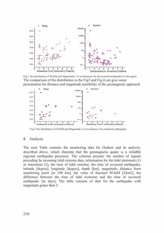
210

Fig.3. the distribution of SChtM and Magnitude (>3) on distances for all occurred earthquakes in the region The comparison of the distribution in the Fig3 and Fig.4 can give some presentation for distance and magnitude sensibility of the geomagnetic approach.

Fig.4. the distribution of SChtM and Magnitude (>3) on distances for predicted earthquakes

5. Analysis

The next Table contains the monitoring data for Dusheti and its analysis, described above, which illustrate that the geomagnetic quake is a reliable regional earthquake precursor. The columns present: the number of signals preceding he incoming tidal extreme data, information for the tidal minimum (1) or maximum (2), the time of tidal extreme, the time of occurred earthquake, latitude [degree], longitude [degree], depth [km], magnitude, distance from monitoring point [in 100 km], the value of function SChtM [J/km2], the difference between the time of tidal exstreme and the time of occurred earthquake [in days]. The table consists of data for the earthquake with magnitude grater then 3.

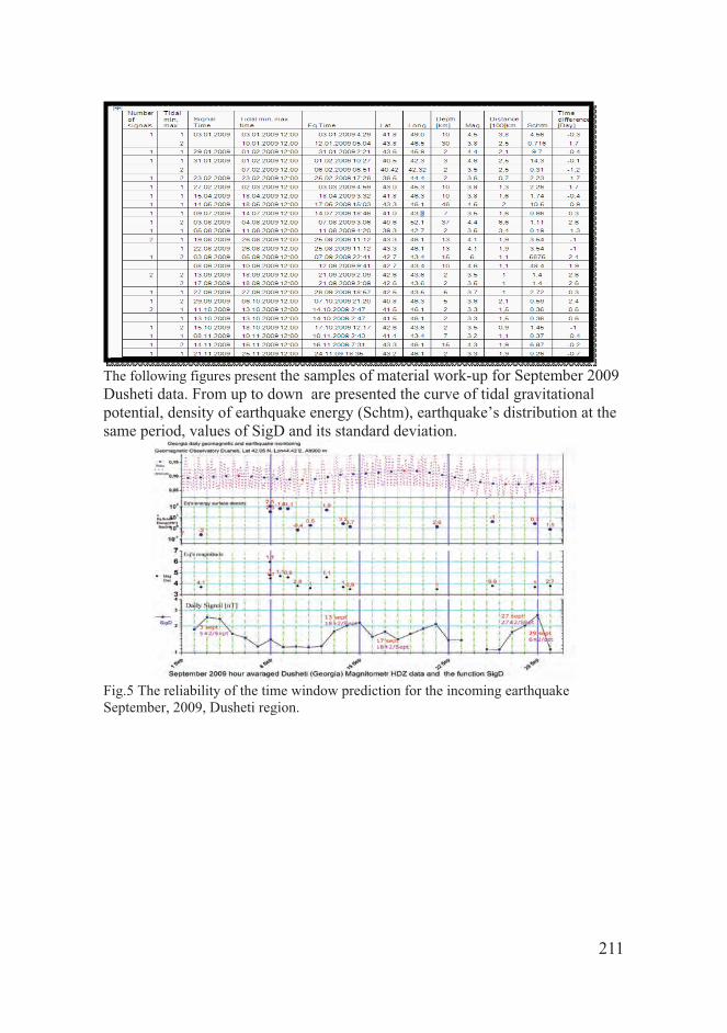
211

The following figures present the samples of material work-up for September 2009 Dusheti data. From up to down are presented the curve of tidal gravitational potential, density of earthquake energy (Schtm), earthquake’s distribution at the same period, values of SigD and its standard deviation.

Fig.5 The reliability of the time window prediction for the incoming earthquake September, 2009, Dusheti region.

212

Fig.6 The ,,monthly monitoring” figure for September, 2009, Dusheti region. Fig.7. Presents the comparison of the number of All occurred and predicted earthquake For Dusheti. Fig7. presents the map graphic for earthquakes with magnitude grater then 4 predicted simultaneously by Dusheti measurement.

Fig.7 Map graphic for earthquakes with magnitude grater then 4 predicted simultaneously by Dusheti measurement. It is clear from the picture that among 12 earthquakes for Mag>4, 8 of them were fixed by us. For the rest 4 earthquakes periods we do not have geomagnetic field data.

It is obvious that the occurred in the predicted time period earthquake with maximum value of function SChtM (proportional to the Richter energy density in the monitoring point) is the predicted earthquake. But sometimes there are more than one geomagnetic signals in one day or some in different days. It is not possible to perform unique interpretation and to choose the predicted earthquakes between some of them with less values of energy density. The solution of this problem can be given by the analysis of the vector geomagnetic monitoring data in at least 3 points, which will permit to start solving the inverse

213

problem for estimation the coordinates of geomagnetic quake source as function of geomagnetic quake. The numbering of powers of freedom for estimation of the epicenter, depth, magnitude and intensity (maximum values of accelerator vector and its dangerous frequencies) and the number of possible earthquake precursors show that the nonlinear system of inverse problem will be over determinate.

5. Conclusion The correlations between the local geomagnetic quake and incoming

earthquakes, which occur in the time window defined from tidal minimum (± 1 day) or maximum (± 2 days) of the Earth tidal gravitational potential are tested statistically. The distribution of the time difference between predicted and occurred events is going to be Gaussian with the increasing of the statistics.

The presented results can be interpreted as a first reliable approach for solving the “when” earthquakes prediction problem by using geomagnetic data. 6. References 1)Aki K., Earthquake prediction, societal implications, U.S. National Report to IUGG, 1991-1994, Rev. Geo-phys. Vol. 33 Suppl., © 1995 American Geophysical Union, http://www.agu.org/revgeophys/aki00/aki00.html , 1995. 2)Freund F.T., A.Takeuchi, B. W.S. Lau, Electric Currents Streaming out of Stressed Igneous Rocks – A Step Towards Understanding Pre-Earthquake Low Frequency EM Emissions, Special Issue “Recent Progress in Seismo Electromagnetics”, Guest Editors M. Hayakawa, S. Pulinets, M. Parrot, and O. A. Molchanov, Phys. Chem. Earth, 2006 3)Duma G., Modeling the impact of telluric currents on earthquake activity, EGU06-A-01730; NH4.01-1TH5P-0571, Vienna, 2006 4) Eftaxias K., P.Kapiris, J.Polygiannakis, N.Bogris, J.Kopanas, G.Antonopoulos, A.Peratzakis and V.Had-jicontis, Signature of pending earthquake from electro-magnetic anomalies, Geophysical Research Letters, Vol.28, No.17, pp.3321-3324, September 2001. 5)Eftaxias K., P.Kapiris, E.Dologlou, J.Kopanas, N.Bogris, G.Antonopoulos, A.Peratzakis and V.Hadjicontis, EM anomalies before the Kozani earthquake: A study of their behaviour through laboratory experiments, Geophysical Research Letters, Vol. 29, No.8 10.1029/ 2001 GL013786, 2002. 6)Ludwin, R.S., 2001, Earthquake Prediction, Washing-ton Geology, Vol. 28, No. 3, May 2001, p. 27, 2001. 7)Mavrodiev S.Cht., Thanassoulas C., Possible correlation between electromagnetic earth fields and future earthquakes, INRNE-BAS, Seminar proceedings, 23- 27 July 2001, Sofia, Bulgaria, ISBN 954-9820-05-X, 2001, http://arXiv.org/abs/physics/0110012, 2001. 8)Mavrodiev S.Cht., On the Reliability of the Geomagnetic Quake Approach as Short Time Earthquake’s Precursor for Sofia Region, Natural Hazards and Earth System Science, Vol. 4, pp 433-447, 21-6-2004 9) Mavrodiev S.Cht., Pekevski, L., and Jimsheladze T., 2008, Geomagnetic-Quake as Iminent Reliable Earthquake’s Preqursor: Starting point Future

214

Complex Regional Network, Electromagnetic Phenomena related to earthquake s and volcanoes. Editor: Birbal Singh. Publ., Narosa Pub.House, new Delhi, pp. 116-134. 10)Pakiser L, Shedlock K.M., Predicting earthquakes, USGS, http://earthquake.usgs.gov/hazards/prediction.html, 1995. 11)St-Laurent F., J. S. Derr, Freund F. T. , Earthquake Lights and the Stress-Activation of Positive Hole Charge Carriers in Rocks, Special Issue “Recent Progress in Seismo Electromagnetics”, Guest Editors M. Hayakawa, S. Pulinets, M. Parrot, and O. A. Molchanov, Phys. Chem. Earth, 2006 12)Thanassoulas, C., Determination of the epicentral area of three earthquakes (Ms>6R) in Greece, based on electrotelluric currents recorded by the VAN network., Acta Geophysica Polonica, Vol. XXXIX, no. 4, 373-387, 1991.