complex numbers and ordinary differential equations

Complex Numbers

and

Ordinary Differential Equations

F Hautmann

Oxford UniversityMichaelmas Term 2011

Books: The material of this course is covered well in many texts on mathematicalmethods for science students, for example Mathematical Methods for Physics and Engi-

neering, Riley, Hobson, Bence (Cambridge University Press) or Mathematical Methods

in the Physical Sciences, Boas (Wiley), both of which provide many examples. A moreelementary book is Stephenson, Mathematical Methods for Science Students (Long-mans). The book by Louis Lyons, All you ever wanted to know about Mathematics

but were afraid to ask (Vol I, CUP, 1995) also provides an excellent treatment of thesubject. I am grateful to James Binney and Graham Ross for providing past courses’material on which these lecture notes are based.

1 Complex Numbers I : Friendly ComplexNumbers

Complex numbers are widely used in physics. The solution of physical equations is oftenmade simpler through the use of complex numbers and we will study examples of thiswhen solving differential equations later in this course. Another particularly importantapplication of complex numbers is in quantum mechanics where they play a centralrole representing the state, or wave function, of a quantum system. In this courseI will give a straightforward introduction to complex numbers and to simple functionsof a complex variable. The first Section “Friendly Complex Numbers” is intended toprovide a presentation of basic definitions and properties of complex numbers suitablefor those who have not studied the subject.

1.1 Why complex numbers?

The obvious first question is “Why introduce complex numbers?”. The logical progres-sion follows simply from the need to solve equations of increasing complexity. Thus westart with natural numbers N (positive integers) 1, 2, 3, . . .

But 20 + y = 12 ⇒ y = −8 → integers Z . . . ,−3,−2,−1, 0, 1, 2, . . .

But 4x = 6 ⇒ x = 32 → rationals Q

But x2 = 2 ⇒ x =√2 → irrationals → reals R (rationals and

irrationals)

But x2 = −1 ⇒ x = i → complex numbers CMultiples of i are called pure imaginary numbers. A general complex number

is the sum of a multiple of 1 and a multiple of i such as z = 2 + 3i. We often use thenotation z = a + ib, where a and b are real. (Sometimes the symbol j instead if i isused - for example in circuit theory where i is reserved for a current.)

We define operators for extracting a, b from z: a ≡ ℜe(z), b ≡ ℑm(z). We call athe real part and b the imaginary part of z.

1.2 Argand diagram (complex plane)

Complex numbers can be represented in the (x,y) plane. Thus the complex numberz = a+ ib → point (a, b) in the ”complex” plane (or ”Argand diagram”):

2 Chapter 1: Complex Numbers I : Friendly Complex Numbers

Using polar co-ordinates the point (a, b) can equivalently be represented by its(r, θ) values. Thus with arg(z) ≡ θ = arctan(b/a) we have

z = |z|(cos θ + i sin θ) ≡ r(cos θ + i sin θ) (1.1).

Note that the length or modulus of the vector from the origin to the point (a, b) isgiven by

|z| ≡ r =√a2 + b2 (1.2).

As we will show in the next section, cos θ + i sin θ = eiθ, the exponential of acomplex argument. So an equivalent way of writing the polar form is

z = reiθ. (1.3)

It is important to get used to this form as it proves to be very useful in many applica-tions. Note that there are an infinite number of values of θ which give the same valuesof cos θ and sin θ because adding an integer multiple of 2π to θ does not change them.Often one gives only one value of θ when specifying the complex number in polar formbut, as we shall see, it is important to include this ambiguity when for instance takingroots or logarithms of a complex number.

It also proves useful to define the complex conjugate z∗ of z by reversing thesign of i, i.e.

z∗ ≡ a− ib (1.4).

The complex numbers z∗ and −z are also shown in the figure. We see that taking thecomplex conjugate z∗ of z can be represented by reflection with respect to the realaxis.

Example 1.1Express z ≡ a + ib = −1 − i in polar form. Here r =

√2 and arctan(b/a) =

arctan 1 = π/4. However it is necessary to identify the correct quadrant for θ.

1.4 Multiplication and division 3

Since a and b are both negative so too are cos θ and sin θ. Thus θ lies in the thirdquadrant θ = 5π

4 + 2nπ where n is any positive or negative integer. Thus finally

we have z =√2ei

5π4+2nπ, n = 0,±1,±2, · · ·, where we have made the ambiguity in

the phase explicit.

In the next two subsections we describe the basic operations of addition andmultiplication with complex numbers.

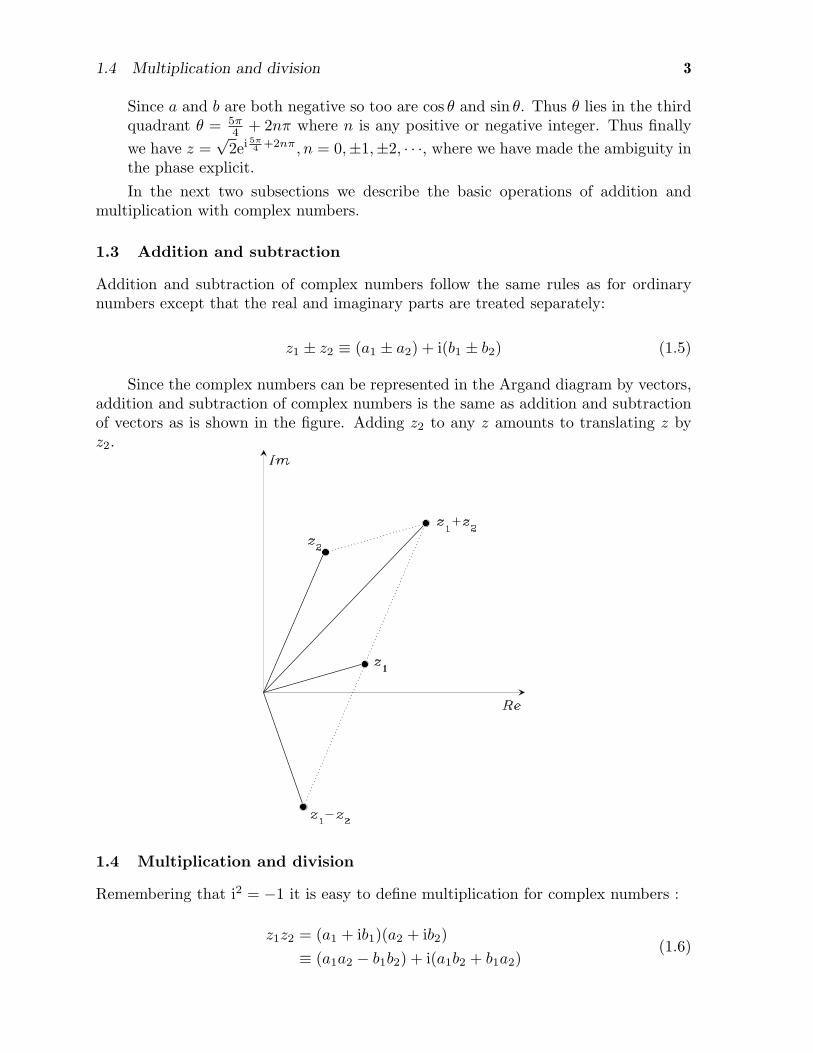
1.3 Addition and subtraction

Addition and subtraction of complex numbers follow the same rules as for ordinarynumbers except that the real and imaginary parts are treated separately:

z1 ± z2 ≡ (a1 ± a2) + i(b1 ± b2) (1.5)

Since the complex numbers can be represented in the Argand diagram by vectors,addition and subtraction of complex numbers is the same as addition and subtractionof vectors as is shown in the figure. Adding z2 to any z amounts to translating z byz2.

1.4 Multiplication and division

Remembering that i2 = −1 it is easy to define multiplication for complex numbers :

z1z2 = (a1 + ib1)(a2 + ib2)

≡ (a1a2 − b1b2) + i(a1b2 + b1a2)(1.6)


Note that the product of a complex number and its complex conjugate, |z|2 ≡zz∗ = (a2+ b2), is real (and ≥ 0) and, c.f. eq (1.2), is given by the square of the lengthof the vector representing the complex number zz∗ ≡ |z|2 = (a2 + b2).

It is necessary to define division also. This is done by multiplying the numeratorand denominator of the fraction by the complex conjugate of the denominator :

z1z2

=z1z

∗2

z2z∗2=z1z

∗2

|z2|2(1.7)

One may see that division by a complex number has been changed into multipli-cation by a complex number. The denominator in the right hand side of eq (1.7) hasbecome a real number and all we now need to define complex division is the rule formultiplication of complex numbers.

Multiplication and division are particularly simple when the polar form of thecomplex number is used. If z1 = |z1|eiθ1 and z2 = |z2|eiθ2 , then their product is givenby

z1 ∗ z2 = |z1| ∗ |z2|ei(θ1+θ2). (1.8)

To multiply any z by z2 = |z2|eiθ2 means to rotate z by angle θ2 and to dilate its lengthby |z2|.

To determine z1z2

note that

z = |z|(cos θ + i sin θ) = |z|eiθ

z∗ = |z|(cos θ − i sin θ) = |z|e−iθ

1

z=

z∗

zz∗=

e−iθ

|z| .(1.9)

Thus

z1z2

=|z1|eiθ1 ∗ e−iθ2

|z2|

=|z1||z2|

ei(θ1−θ2)(1.10)

1.4.1 Graphical representation of multiplication & division

z1z2 = |z1||z2|ei(θ1+θ2)

1.4 Multiplication and division 5

z1z2

=|z1||z2|

ei(θ1−θ2)

Example 1.2

Find the modulus |z1/z2| when{z1 = 1 + 2iz2 = 1− 3i

Clumsy method:∣∣∣∣z1z2

∣∣∣∣ =∣∣∣∣1 + 2i

1− 3i

∣∣∣∣ =|z1z∗2 ||z2|2

=|(1 + 2i)(1 + 3i)|

1 + 9=

|(1− 6) + i(2 + 3)|10

=

√25 + 25

10=

√2

2=

1√2

Elegant method: ∣∣∣∣z1z2

∣∣∣∣ =|z1||z2|

=

√1 + 4√1 + 9

=1√2


Methods based on complex addition and multiplication can be useful to analyzeplane geometry problems as in the following example.

Example 1.3Consider an arbitrary quadrilateral and construct squares on each side as in thefigure below. Show that segments joining the centres of opposite squares areperpendicular and of equal length.

2a+2b+2c+2d=0

p

r

s

q

2a

2b

2c

0

2d

Consider the complex plane and let the vertices of the quadrilateral be at points 2a,2a+ 2b, 2a+ 2b+ 2c, and 2a+ 2b+ 2c+ 2d = 0. The centre of the square on the firstside is at

p = a+ aeiπ/2 = a(1 + i) .

Likewise, the centres of the other squares are at

q = 2a+ b(1 + i) , r = 2a+ 2b+ c(1 + i) , s = 2a+ 2b+ 2c+ d(1 + i) .

Thus

A ≡ s− q = b(1− i) + 2c+ d(1 + i) , B ≡ r − p = a(1− i) + 2b+ c(1 + i) .

A and B perpendicular and of equal length means B = Aeiπ/2, i.e., B = iA, i.e.,A+ iB = 0. We verify that this is indeed the case:

A+ iB = b(1− i) + 2c+ d(1 + i) + ia(1− i) + 2ib+ ic(1 + i)

= b(1 + i) + c(1 + i) + d(1 + i) + a(1 + i) = (1 + i)(a+ b+ c+ d) = 0 .

2.1 Elementary functions of complex variable 7

2 Complex Numbers II

This section is devoted to basic functions of complex variable and simple applications.We give de Moivre’s theorem and show examples of its uses. We introduce the notionof curves in the complex plane. We end by discussing applications of complex variableto finding roots of polynomials.

2.1 Elementary functions of complex variable

We may define polynomials and rational functions of complex variable z based on thealgebraic operations of multiplication and addition of complex numbers introduced inthe previous section. For example, separating real and imaginary parts, z = x+ iy, wehave

f(z) = z2 = (x+ iy)(x+ iy) = x2 − y2 + 2ixy .

Similarly,

f(z) =1

z=

z∗

|z|2 =x

x2 + y2− i

y

x2 + y2.

To define the complex exponential and related functions such as trigonometric andhyperbolic functions, we use power series expansion.

2.1.1 The complex exponential function

The definition of the exponential, cosine and sine functions of a real variable canbe done by writing their series expansions :

ex = 1 + x+x2

2!+ · · ·+ xn

n!+ · · ·

cosx = 1− x2

2!+x4

4!− · · ·+ (−1)n

x2n

(2n)!+ · · ·

sinx = x− x3

3!+x5

5!− · · ·+ (−1)n

x2n+1

(2n+ 1)!+ · · ·

(2.1)

For small x a few of terms may be sufficient to provide a good approximation. Thusfor very small x, sinx ≈ x.

In a similar manner we may define functions of the complex variable z. Thecomplex exponential is defined by

ez = 1 + z +z2

2!+ · · · (2.2)

A special case is if z is purely imaginary z = iθ. Using the fact that i2n = 1 or −1 forn even or odd and i2n+1 = i or −i for n even or odd we may write

eiθ =(1− θ2

2!+θ4

4!+ · · ·

)+ i(θ − θ3

3!+ · · ·

)

= cos θ + i sin θ

(2.3)

8 Chapter 2: Complex Numbers II

This is the relation that we used in writing a complex number in polar form, c.f. eq(1.3). Thus

z = |z|(cos θ + i sin θ) = |z|eiθ

z∗ = |z|(cos θ − i sin θ) = |z|e−iθ

1

z=

z∗

zz∗=

e−iθ

|z| .(2.4)

We may find a useful relation between sines and cosines and complex exponentials.Adding and then subtracting the first two of equations (2.4) we find that

cos θ = 12 (e

iθ + e−iθ)

sin θ = 12i (e

iθ − e−iθ)(2.5)

2.1.2 The complex sine and cosine functions

In a similar manner we can define cos z and sin z by replacing the argument x in(2.1) by the complex variable z. The analogue of de Moivre’s theorem is

eiz =(1− z2

2!+z4

4!+ · · ·

)+ i(z − z3

3!+ · · ·

)

= cos z + i sin z

(2.6)

Similarly one hascos z = 1

2 (eiz + e−iz)

sin z = 12i (e

iz − e−iz)(2.7)

From this we learn that the cosine and the sine of an imaginary angle are

cos(ib) = 12 (e

−b + eb) = cosh b

sin(ib) = 12i (e

−b − eb) = i sinh b,(2.8)

where we have used the definitions of the hyperbolic functions

cosh b ≡ 12 (e

b + e−b)

sinh b ≡ 12 (e

b − e−b).(2.9)

Note:

Hyperbolic functions get their name from the identity cosh2 θ− sinh2 θ = 1, whichis readily proved from (2.9) and is reminiscent of the equation of a hyperbola,x2 − y2 = 1.

2.1.3 Complex hyperbolic sine and cosine functions

We define complex hyperbolic functions in a similar manner as done above forcomplex trigonometric functions, by replacing the real argument in the power seriesexpansion by complex variable z. Then we have

cosh z = 12 (e

z + e−z)

sinh z = 12 (e

z − e−z).(2.10)

2.3 Uses of de Moivre’s theorem 9

2.2 de Moivre’s theorem and trigonometric identities

Using the rules for multiplication of complex numbers gives the general form of deMoivre’s theorem :

zn = (reiθ)n = rneinθ = rn(cosnθ + i sinnθ) (2.11)

for any integer n. That is,

(eiθ)n = (cos θ + i sin θ)n = cosnθ + i sinnθ. (2.12)

2.2.1 Trigonometric identities

Eq (2.12) generates simple identities for cosnθ and sinnθ. For example, for n = 2we have, equating the real and imaginary parts of the equation

cos 2θ = cos2 θ − sin2 θ

sin 2θ = 2 cos θ sin θ(2.13)

The complex exponential is very useful in establishing trigonometric identities.We have

cos(a+ b) + i sin(a+ b) = ei(a+b) = eiaeib

= (cos a+ i sin a)(cos b+ i sin b)

= (cos a cos b− sin a sin b) + i(cos a sin b+ sin a cos b)

(2.14)

where we have used the property of exponentials that ei(a+b) = eiaeib. This is anexample of a complex equation relating a complex number on the left hand size (LHS)to a complex number on the right hand side (RHS). To solve it we must equate thereal parts of the LHS and the RHS and separately the imaginary parts of the LHS andRHS. Thus a complex equation is equivalent to two real equations. Comparing realand imaginary parts on the two sides of (2.14), we deduce that

cos(a+ b) = cos a cos b− sin a sin b

sin(a+ b) = sin a cos b+ cos a sin b

2.2.2 Identities for complex sines and cosines

We may use the result of (2.7) to evaluate the cosine of a complex number:

cos z = cos(a+ ib)

= 12 (e

(ia−b) + e(−ia+b))

= 12 (e

−b(cos a+ isina) + eb(cos a− i sin a))

= cos a cosh b− i sin a sinh b.

(2.15)

Analogouslysin z = sin a cosh b+ i cos a sinh b. (2.16)


2.3 Uses of de Moivre’s theorem

It is often much easier and more compact to work with the complex exponential ratherthan with sines and cosines. Here I give just three examples; you will encounter morein the discussion of differential equations and in the problem sets.

Example 2.1Find (1 + i)8. Taking powers is much simpler in polar form so we write (1 + i) =√(2)eiπ/4. Hence (1 + i)8 = (

√(2)eiπ/4)8 = 16e2πi = 16.

Example 2.2Solving differential equations is often much simpler using complex exponentials aswe shall discuss in detail in later lectures. As an introductory example I consider

here the solution of simple harmonic motion, d2ydθ2 + y = 0. The general solution is

well known y = A cos θ + B sin θ where A and B are real constants. To solve itusing the complex exponential we first write y = ℜez so that the equation becomesd2ℜezdθ2 +ℜez = ℜe(d

2zdθ2 + z) = 0 The solution to the equation d2z

dθ2 + z = 0 is simplyz = Ceiθ where C is a (complex) constant. (You may check that this is the casesimply by substituting the answer in the original equation). Writing C = A− iBone finds, using de Moivre,

y = ℜez = ℜe((A− iB)(cos θ + i sin θ))

= A cos θ +B sin θ(2.17)

Thus we have derived the general solution in one step - there is no need to lookfor the sine and cosine solutions separately. Although the saving in effort throughusing complex exponentials is modest in this simple example, it becomes significantin the solution of more general differential equations.

Example 2.3Series involving sines and cosines may often be summed using de Moivre. As anexample we will prove that for 0 < r < 1

∞∑

n=0

rn sin(2n+ 1)θ =(1 + r) sin θ

1− 2r cos 2θ + r2

Proof:∞∑

n=0

rn sin(2n+ 1)θ =∑

n

rnℑm(ei(2n+1)θ) = ℑm

(eiθ∑

n

(re2iθ)n)

= ℑm

(eiθ

1

1− re2iθ

)

= ℑm

(eiθ(1− re−2iθ)

(1− re2iθ)(1− re−2iθ)

)

=sin θ + r sin θ

1− 2r cos 2θ + r2

2.4 Complex logarithm 11

2.4 Complex logarithm

The logarithmic function f(z) = ln z is the inverse of the exponential function meaningthat if one acts on z by the logarithmic function and then by the exponential functionone gets just z, eln z = z. We may use this property to define the logarithm of acomplex variable :

eln z = z = |z|eiθ = eln |z|eiθ = eln |z|+iθ

⇒ ln z = ln |z|+ i arg(z)

(a) (b)

(2.18)

Part (a) is just the normal logarithm of a real variable and gives the real part of thelogarithmic fiunction while part (b) gives its imaginary part. Note that the infiniteambiguity in the phase of z is no longer present in ln z because the addition of an integermultiple of 2π to the argument of z changes the imaginary part of the logarithm bythe same amount. Thus it is essential, when defining the logarithm, to know preciselythe argument of z. We can rewrite Eq (2.18) explicitly as

ln z = ln |z|+ i(θ + 2πn) , n integer . (2.19)

For different n we get different values of the complex logarithm. So we need to assignn to fully specify the logarithm.

The different values corresponding to different n are called “branches” of thelogarithm. n = 0 is called the principal branch.

A function of z which may take not one but multiple values for a given value of zis called multi-valued. The logarithm is our first example of a multi-valued function.

Example 2.4Find all values of ln(−1).

ln(−1) = ln eiπ = ln 1 + i(π + 2πn) = iπ + 2πin , n integer .

For the principal branch n = 0

ln(−1) = iπ (n = 0) .

Note:

eln z always equals z, while ln ez does not always equal z.

Let z = a+ ib = reiθ. Then ln z = ln r + i(θ + 2πn) , n integer. So

eln z = eln r+i(θ+2πn) = reiθ e2πni︸︷︷︸1

= reiθ = z .

On the other hand ez = ea+ib = eaeib. Therefore

ln ez = ln ea + i(b+ 2πn) = a+ ib︸︷︷︸z

+2πin = z + 2πin which may be 6= z .


2.4.1 Complex powers

Once we have the complex logarithm, we can define complex powers f(z) = zα,where both z and α are complex:

f(z) = zα = eα ln z . (2.20)

Since the logarithm is multi-valued, complex powers also are multi-valued func-tions.

Example 2.5Show that ii is real and the principal-branch value is ii = 1/

√eπ.

ii = ei ln i = ei[ln 1+i(π/2+2πn)] = e−π/2−2πn.

These values are all real. For n = 0 we have ii = e−π/2 = 1/√eπ.

2.5 Curves in the complex plane

The locus of points satisfying some constraint on a complex parameter traces out acurve in the complex plane. For example the constraint |z| = 1 requires that the lengthof the vector from the origin to the point z is constant and equal to 1. This clearlycorresponds to the set of points lying on a circle of unit radius.

Instead of determining the geometric structure of the constraint one may insteadsolve the constraint equation algebraically and look for the equation of the curve.This has the advantage that the method is in principle straightforward although thedetails may be algebraically involved whereas the geometrical construction may not beobvious. In Cartesian coordinates the algebraic constraint corresponding to |z| = 1 is|z|2 = a2 + b2 = 1 which is the equation of a circle as expected. In polar coordinatesthe calculation is even simpler |z| = r = 1.

As a second example consider the constraint |z − z0| = 1. This is the equation ofa unit circle centre z0 as may be immediately seen by changing the coordinate systemto z′ = (z − z0).

Alternatively one may solve the constraint algebraically to find |z − z0|2 = (a −a0)

2+(b−b0)2 = 1 which is the equation of the unit circle centred at the point (a0, b0).The solution in polar coordinates is not so straightforward in this case, showing thatit is important to try the alternate forms when looking for the algebraic solution. Toillustrate the techniques for finding curves in the complex plane in more complicatedcases I present some further examples:

Example 2.6

What is the locus in the Argand diagram that is defined by

∣∣∣∣z − i

z + i

∣∣∣∣ = 1?

Equivalently we have |z − i| = |z + i|, so the distance to z from (0, 1) is the sameas the distance from (0,−1). Hence the solution is the “real axis”.

2.5 Curves in the complex plane 13

Alternatively we may solve the equation

a2 + (b− 1)2 = a2 + (b+ 1)2

which gives b = 0, a arbitrary, corresponding to the real axis.

Example 2.7

What is the locus in the Argand diagram that is defined by arg( z

z + 1

)=π

4?

Equivalently arg(z)− arg(z + 1) =π

4

Solution: “portion of circle through (0, 0) and (−1, 0)”

The x-coordinate of the centre is − 12 by symmetry. The angle subtended by a

chord at the centre is twice that subtended at the circumference, so here it is π/2.With this fact it follows that the y-coordinate of the centre is 1

2 .

Try solving this example algebraically.

The lower portion of circle is arg( z

z + 1

)= −3π

4


Another way to specify a curve in the complex plane is to give its parametric form,namely, a function z = γ(t) that maps points on a real axis interval [a, b] on to pointsin the complex plane C:

γ : t 7→ z = γ(t) = x(t) + iy(t) , a ≤ t ≤ b .

Examples are given in the figure below.

Im z

Im z

Re z

R

Re z

Im z

Re z

x(t) = x

y(t) = y

0 < t < 2

0 + R cos t

0 + R sin t

π

x(t) = x 0 + R1 cos t

y(t) = y0 + R 2 sin t

y(t) = t sin t

x(t) = t cos t

i ti.e., z = t e

The top example is a representation of the circle centred in z0 = x0+ iy0 of radiusR, since it gives

(x− x0)2 + (y − y0)

2 = R2 .

The next example is the ellipse

(x− x0)2

R21

+(y − y0)

2

R22

= 1 .

The third example is a spiral obtained by letting the radius vary with t.

2.5.1 Complex functions as mappings

As discussed earlier on, the topic of this section highlights the intersection ofalgebraic and geometric viewpoints on complex variable. In this perspective it is worthobserving that functions of complex variable

f : z 7→ w = f(z)

can be usefully viewed as mapping sets of points in the complex plane C (e.g. curves,or regions delimited by curves) into other sets of points in C.

For example, take the exponential function

w = f(z) = ez

and ask on to which curves in the complex w plane this function maps straight linesparallel to the real and to the imaginary axes in the complex z plane. To see this, set

z = x+ iy ; w = ρeiφ .

2.6 Roots of polynomials 15

Thenρ = ex ;φ = y .

Thus the exponential maps horizontal lines x = a in the z plane on to circles ρ = ea

in the w plane, and vertical lines y = b in the z plane on to rays φ = b in the w plane.The mapping is illustrated in the figure below.

1

��

��

Im z

Re w

f

Im w

b

b

b2

b1

1

2

Re za a 2

Given a function of complex variable f , for any subset A of C we call the “imageof A through f” the set of points w such that w = f(z) for some z belonging to A,and we denote this by f(A). We say that f maps A on to f(A).

Example 2.8Let f(z) = 1/z. Where does f map the interior and exterior of the unit circle|z| = 1? What does f do to points on the unit circle?

Let w = f(z) =1

z; z = reiθ ⇒ w =

1

re−iθ

1

Im z

Re z

f

Im w

Re w1

f maps the interior of the unit circle on to the exterior, and viceversa. The unitcircle is mapped on to itself.

2.6 Roots of polynomials

Complex numbers enable us to find roots for any polynomial

P (z) ≡ anzn + an−1z

n−1 + · · ·+ a0. (2.21)

That is, there is at least one, and possibly as many as n complex numbers zi such thatP (zi) = 0. Many physical problems involve such roots.

In the case n = 2 you already know a general formula for the roots. There is asimilar formula for the case n = 3 and historically this is important because it leadto the invention of complex numbers. However, it can be shown that such generalformulae do not exist for equations of higher order. We can, however, find the roots ofspecially simple polynomials.

In this section we start by defining and evaluating roots of complex numbers. Thenwe discuss how to characterize polynomials by their roots. Finally we give examples ofhow to use complex variable techniques to solve polynomial equations in special cases.


2.6.1 Roots of complex numbers

A number u is defined to be an n-th root of complex number z if un = z. Thenwe write u = z1/n. The following result obtains.

Every complex number has exactly n distinct n-th roots.

Proof. Let z = r(cos θ + i sin θ); u = ρ(cosα + i sinα). Then, using de Moivre’stheorem,

r(cos θ + i sin θ) = ρn(cosα+ i sinα)n = ρn(cosnα+ i sinnα)

⇒ ρn = r , nα = θ + 2πk (k integer)

Therefore ρ = r1/n , α = θ/n+ 2πk/n .

We thus see that we get n distinct values for k, from 0 to n − 1, corresponding to ndistinct values of u for z 6= 0. So

u = z1/n = r1/n[cos

(θ

n+

2πk

n

)+ i sin

(θ

n+

2πk

n

)], k = 0, 1, . . . , n− 1 . (2.22)

We note that the function f(z) = z1/n is a multi-valued function.

Example 2.9Find all cubic roots of z = −1 + i.

Applying Eq (2.22) we have

u = (−1 + i)1/3

= (√2)1/3

[cos

(3π

4

1

3+

2πk

3

)+ i sin

(3π

4

1

3+

2πk

3

)], k = 0, 1, 2 .

That is, the three cubic roots of −1 + i are

21/6(cos

π

4+ i sin

π

4

)(k = 0) ,

21/6(cos

11π

12+ i sin

11π

12

)(k = 1) ,

21/6(cos

19π

12+ i sin

19π

12

)(k = 2) .

k=2

k=0

k=1


Equivalently, using Eq (2.20),

u = (−1 + i)1/3 = e(1/3) ln(−1+i) = e(1/3)[ln√2+i(3π/4+2kπ)]

= (√2)1/3ei(π/4+2kπ/3) .

2.6.2 Characterizing a polynomial by its roots

Consider a polynomial of degree n in the complex variable z

P (z) ≡ anzn + an−1z

n−1 + · · ·+ a0,

where ak are complex coefficients. z = zi is root of P (z) if P (zi) = 0.

For n = 2 we have the quadratic formula for roots

z1,2 = − a12a2

± 1

2a2

√a21 − 4a0a2 .

The sum and product of the roots are given respectively by

sum of roots = −a1a2

, product of roots =a0a2

. (2.23)

For n = 3 there exists a formula for roots as well. For n > 3 no explicit formulaexists, but there exists a general theorem, the fundamental theorem of algebra (dis-cussed in the course on “Functions of a complex variable”), which states that everynonzero single-variable polynomial P (z) with complex coefficients has exactly as manycomplex roots as its degree (counting repeated roots with their multiplicity). Here weuse this result to notice that we can characterize P (z) equivalently by its coefficientsor by its roots.

More precisely, knowledge of a polynomial’s roots enables us to express the poly-nomial as a product of linear terms

anzn + an−1z

n−1 + · · ·+ a0 = an(z − r1)(z − r2) · · · (z − rn)

= an

(zn − zn−1

n∑

j=1

rj + · · ·+ (−1)nn∏

j=1

rj

).

(2.24)

Comparing the coefficients of zn−1 and z0 on the two sides, we deduce that

an−1

an= −

∑

j

rj ;a0an

= (−1)n∏

j

rj (2.25)

i.e. the two ratios on the left hand sides in Eq (2.25) are related to the sum andthe product of the roots respectively, of which Eq (2.23) is a special case for n = 2.

In what follows we use complex variable techniques to find roots of polynomialsin special cases.


2.6.3 Special polynomials

Let us start with a simple case. Consider

xn = 1 ⇒ x = 11/n

The solution is given by the nth roots of unity. In taking roots it is crucial toallow for the ambiguity in the phase of a (complex) number

1 = e2mπi ⇒ 11/n = e2mπi/n

= cos(2mπ

n

)+ i sin

(2mπn

) (2.26)

E.g. for n = 5

11/5 = cos(2mπ

5

)+ i sin

(2mπ5

)(m = 0, 1, 2, 3, 4).

The roots may be drawn in the Argand plane and correspond to five equally spacedpoints in the plane :

Example 2.10Consider the equation

z5 + 32 = 0 .

This is similar to the previous case. The solutions are the fifth roots of −32:

(−32)1/5 = 321/5[cos

(π

5+

2πk

5

)+ i sin

(π

5+

2πk

5

)], k = 0, 1, 2, 3, 4

that is,

k = 0 : 2(cos π5 + i sin π

5

)

k = 1 : 2(cos 3π

5 + i sin 3π5

)


k = 2 : −2

k = 3 : 2(cos 7π

5 + i sin 7π5

)

k = 4 : 2(cos 9π

5 + i sin 9π5

)

Re z

k=0

k=1

k=2

k=3

k=4

Im z

In what follows I will illustrate the techniques of taking roots in more complicatedcases by a series of examples. In this we shall often need the coefficients of xryn−r in(x+ y)n. These are given by the binomial coefficients

(nr

)=

n!

r!(n− r)!.

Useful mnemonics for these coefficients is represented by the Pascal’s triangle

(x+ y)0

(x+ y)1

(x+ y)2

(x+ y)3

(x+ y)4

(x+ y)5

11 1

1 2 11 3 3 1

1 4 6 4 11 5 10 10 5 1

in which each row is obtained from the one above by adding the numbers to right andleft of the position to be filled in. That is, the r-th element of n-th row is given by thesum of the two elements above it in the (n− 1)-th row:

(nr

)=

(n− 1r − 1

)+

(n− 1r

). (2.27)

Example 2.11Consider the equation

(z + i)7 + (z − i)7 = 0.


This may be solved by the techniques just discussed as follows:

(z + i

z − i

)7

= −1 = e(2m+1)πi

⇒ z + i

z − i= e(2m+1)πi/7 ⇒ z

(1− e(2m+1)πi/7

)= −i

(1 + e(2m+1)πi/7

)

⇒ z = ie(2m+1)πi/7 + 1

e(2m+1)πi/7 − 1= i

e(2m+1)πi/14 + e−(2m+1)πi/14

e(2m+1)πi/14 − e−(2m+1)πi/14= i

2 cos(

2m+114 π

)

2i sin(

2m+114 π

) .

Thus

z = cot(2m+ 1

14π), m = 0, 1, 2, 3, 4, 5, 6 .

The original equation can be written in another form

⇒ z7 − 21z5 + 35z3 − 7z = 0

⇒ z6 − 21z4 + 35z2 − 7 = 0 or z = 0

⇒ w3 − 21w2 + 35w − 7 = 0 (w ≡ z2)

Thus, using our solution for the roots of the original equation, we see the roots of

w3 − 21w2 + 35w − 7 = 0 are w = cot2(2m+114 π

)(m = 0, 1, 2).

Example 2.12Sometimes the underlying equation which can be solved by these techniques is notobvious. For example - find the roots of

z3 + 7z2 + 7z + 1 = 0.

If one writes three more rows in the Pascal’s triangle given in the previous pageusing the rule in Eq. (2.27), one finds that the ninth row is

1 8 28 56 70 56 28 8 1,

so12 [(z + 1)8 − (z − 1)8] = 8z7 + 56z5 + 56z3 + 8z

= 8z[w3 + 7w2 + 7w + 1] (w ≡ z2).

Now (z + 1)8 − (z − 1)8 = 0 whenz + 1

z − 1= e2mπi/8, i.e. when

z =emπi/4 + 1

emπi/4 − 1= −i cot(mπ/8) (m = 1, 2, . . . , 7),

so the roots of the given equation are z = − cot2(mπ/8), m = 1, 2, 3.


Example 2.13Show that

∑2m=0 cot

2(2m+114 π

)= 21

Solution: From Example 2.11 we have that the left hand side is the sum of theroots of w3 − 21w2 +35w− 7 = 0. Then the result follows from the first equationin (2.25).

Example 2.14Note that based on eq (2.24) a polynomial may be characterized by (i) its rootsand (ii) any an. To illustrate the use of this representation show that

z2m − a2m

z2 − a2=(z2−2az cos

π

m+a2

)(z2−2az cos

2π

m+a2

)· · ·(z2−2az cos

(m− 1)π

m+a2

).

Solution: Consider P (z) ≡ z2m−a2m, a polynomial of order 2m with leading terma2m = 1 and roots zr = aerπi/m. Define

Q(z) ≡ (z2−a2)(z2−2az cos

π

m+a2

)(z2−2az cos

2π

m+a2

)· · ·(z2−2az cos

(m− 1)π

m+a2

).

This polynomial is of order 2m with leading coeff. a2m = 1 and with roots thatare the numbers

zr = a cosrπ

m±√a2 cos2

rπ

m− a2

= a(cos

rπ

m± i

√1− cos2

rπ

m

)= ae±irπ/m (r = 0, 1, . . . ,m).

Thus P and Q are identical.

22 Chapter 3: Differential Equations I

3 Differential Equations I

A differential equation is an equation in which an expression involving deriva-tives of an unknown function is set equal to a known function. For example

df

dx+ xf = sinx (3.1)

is a differential equation for f(x). To determine a unique solution of a differentialequation we require some initial data; in the case of (3.1), the value of f at some pointx. These data are often called initial conditions. Below we’ll discuss how manyinitial conditions one needs.

Differential equations enable us to encapsulate physical laws: the equation governsevents everywhere and at all times; the rich variety of experience arises because atdifferent places and times different initial conditions select different solutions. Sincedifferential equations are of such transcending importance for physics, let’s talk aboutthem in some generality. In this course we will talk of ordinary differential equations(ODE): namely, equations involving derivatives with respect to one single variable (asopposed to partial differential equations, involving derivatives with respect to morethan one variable).

3.1 Differential operators

Every differential equation involves a differential operator.

functions: numbers → numbers (e.g. x → ex)

operators: functions → functions (e.g. f → αf ; f → 1/f ; f → f + α; . . .)

A differential operator does this mapping by differentiating the function one ormore times (and perhaps adding in a function, or multiplying by one, etc).

(e.g. f → df

dx; f → d2f

dx2; f → 2

d2f

dx2+ f

df

dx; . . .

)

It is useful to name the operators. For example we could denote by L(f) the

operation f → df

dx.

3.1.1 Order of a differential operator

The order of a differential operator is the order of the highest derivative containedin it. So

L1(f) ≡df

dx+ 3f is first order,

L2(f) ≡d2f

dx2+ 3f is second order,

L3(f) ≡d2f

dx2+ 4

df

dxis second order.

3.3 Inhomogeneous terms 23

3.1.2 Linear operators

L is a linear operator if

L(αf + βg) = αL(f) + βL(g), (3.2)

where α and β are (possibly complex) numbers.(e.g. f → df

dxand f → αf are linear, but f → 1

fand f → f + α are not.

)

3.2 Linearity

An expression of the type αf + βg that is a sum of multiples of two or morefunctions is called a linear combination of the functions.

To a good approximation, many physical systems are described by linear differ-ential equations L(f) = 0. Classical electrodynamics provides a notable example: theequations (Maxwell’s) governing electric and magnetic fields in a vacuum are linear.The related equation governing the generation of a Newtonian gravitational field isalso linear. Similarly in quantum mechanics the differential equations governing theevolution of the system, such as the Schrodinger equation, are linear.

Suppose f and g are two solutions of the linear equation L(y) = 0 for differentinitial conditions. For example, if L symbolizes Maxwell’s equations, f and g mightdescribe the electric fields generated by different distributions of charges. Then since Lis linear, L(f + g) = 0, so (f + g) describes the electric field generated by both chargedistributions taken together. This idea, that if the governing equations are linear,then the response to two stimuli taken together is just the sum of the responses to thestimuli taken separately, is known as the principle of superposition. This principleis widely used to find the required solution to linear differential equations: we start byfinding some very simple solutions that individually don’t satisfy our initial conditionsand then we look for linear combinations of them that do.

Linearity is almost always an approximation that breaks down if the stimuli arevery large. For example, in consequence of the linearity of Maxwell’s equations, thebeam from one torch will pass right through the beam of another torch without beingaffected by it. But the beam from an extremely strong source of light would scatter atorch beam because the vacuum contains ‘virtual’ electron-positron pairs which respondnon-negligibly to the field of a powerful beam, and the excited electron-positron pairscan then scatter the torch beam. In a similar way, light propagating through a crystal(which is full of positive and negative charges) can rather easily modify the electricalproperties of a crystal in a way that affects a second light beam – this is the ideabehind non-linear optics, now an enormously important area technologically. Gravitytoo is non-linear for very strong fields.

While non-linearity is the generic case, the regime of weak stimuli in which physicsis to a good approximation linear is often a large and practically important one. More-over, when we do understand non-linear processes quantitatively, this is often doneusing concepts that arise in the linear regime. For example, any elementary particle,such as an electron or a quark, is a weak-field, linear-response construct of quantumfield theory.


3.3 Inhomogeneous terms

We’ve so far imagined the stimuli to be encoded in the initial conditions. It is sometimesconvenient to formulate a physical problem so that at least some of the stimuli areencoded by a function that we set our differential operator equal to. Thus we write

Lgiven

(f) =sought

homogeneous

h(x)given

inhomogeneous(3.3)

If h(x) = 0, Eq. (3.3) is homogeneous. If h(x) 6= 0, it is nonhomogeneous.

Suppose f1 is the general solution of Lf = 0 and f0 is any solution of Lf = h. Wecall f1 the complementary function and f0 the particular integral and then thegeneral solution of Lf = h is

f1 + f0.Complementary fn Particular integral

(3.4)

How many initial conditions do we need to specify to pick out a unique solution ofL(f) = 0? It is easy to determine this in a hand-waving way because the solutionto a differential equation requires integration. With a single derivative one needs toperform one integration which introduces one integration constant which in turn mustbe fixed by one initial condition. Thus the number of integration constants needed,or equivalently the number of initial conditions, is just the order of the differentialequation. A more rigorous justification of this may be found in Sec. 3.5.

3.4 First-order linear equations

Any first-order linear equation can be written in the form

df

dx+ q(x)f = h(x). (3.5)

Since the solution to this equation implies an integration to remove the derivative thegeneral solution will have one arbitrary constant. The solution can be found by seekinga function I(x) such that

Idf

dx+ Iqf =

dIf

dx= Ih ⇒ f(x) =

1

I(x)

[∫I(x)h(x)dx+ C

]. (3.6)

C is the required arbitrary constant in the solution, and I is called the integratingfactor. We need Iq = dI/dx, so

ln I =

∫q dx ⇒ I = e

∫q dx. (3.7)

Example 3.1Solve

2xdf

dx− f = x2.

3.5 Arbitrary constants & general solutions 25

In standard form the equation reads

df

dx− f

2x= 1

2x

so q = − 1

2xand by (3.7) I = e−

12ln x =

1√x.

Plugging this into (3.6) we have f =√x[

∫12

√x dx+ C] = 1

3x2 + Cx1/2.

Example 3.2Solve the equation

df

dx+ 2f = x2

with the initial conditionf(3) = 0 .

Solution. The integrating factor is given by

I(x) = e∫

2 dx = e2x .

Thus the general solution is

f(x) = e−2x[

∫dx x2e2x + const.]

= e−2x [e2xx2 − x+ 1/2

2+ const.] .

The initial condition f(3) = 0 requires

e−6 [e613

4+ const.] = 0 ,

that is, const. = −e6 13/4. Therefore

f(x) =x2 − x+ 1/2

2− 13

4e6−2x .

3.5 Arbitrary constants & general solutions

We have seen that the general solution of a first-order linear ODE depends onone arbitrary constant, and one initial condition is needed to determine the solutionuniquely. How many initial conditions do we need to specify to pick out a uniquesolution of an nth-order linear ODE L(f) = 0? Arrange Lf ≡ anf

(n) + an−1f(n−1) +

· · ·+ a0f = 0 as

f (n)(x) = −(an−1

anf (n−1)(x) + · · ·+ a0

anf

). (3.8)


If we differentiate both sides of this equation with respect to x, we obtain an expressionfor f (n+1)(x) in terms of f (n)(x) and lower derivatives. With the help of (3.8) we caneliminate f (n)(x) from this new equation, and thus obtain an expression for f (n+1)(x)in terms of f(x) and derivatives up to f (n−1)(x). By differentiating both sides of ournew equation and again using (3.8) to eliminate f (n) from the resulting equation, wecan obtain an expression for f (n+2)(x) in terms of f(x) and derivatives up to f (n−1)(x).Repeating this procedure a sufficient number of times we can obtain an expression forany derivative of f in terms of f(x) and derivatives up to f (n−1). Consequently, if thevalues of these n functions are given at any point x0 we can evaluate the Taylor series

f(x) = f(x0) + (x− x0)f′(x0) +

12 (x− x0)

2f ′′(x0) + · · · (3.9)

for any value of x that lies near enough to x0 for the series to converge. Consequently,the functional form of f(x) is determined by the original nth order differential equationand the n initial conditions f(x0), . . . , f

(n−1)(x0). Said another way, to pick out aunique solution to an nth order equation, we need n initial conditions.

The general solution of a differential equation is one that contains a sufficientsupply of arbitrary constants to allow it to become any solution of the equation ifthese constants are assigned appropriate values. We have seen that once the n numbersf (r)(x0) for r = 0, . . . , n − 1 have been specified, the solution to the linear nth-orderequation Lf = 0 is uniquely determined. This fact suggests that the general solutionof Lf = 0 should include n arbitrary constants, one for each derivative. This is true,although the constants don’t have to be the values of individual derivatives; all thatis required is that appropriate choices of the constants will cause the rth derivative ofthe general solution to adopt any specified value.

Given the general solution we can construct n particular solutions f1, . . . , fn asfollows: let f1 be the solution in which the first arbitrary constant, k1, is unity andthe others zero, f2 be the solution in which the second constant, k2, is unity and theother zero, etc. It is easy to see that the general solution is

f(x) =

n∑

r=1

krfr(x). (3.10)

That is, the general solution is a linear combination of n particular solutions, thatis, solutions with no arbitrary constant.

3.6 First-order non-linear equations

The general form of a first-order differential equation for a function y = f(x) canbe written as a relationship between x, y, and the first derivative y′ = dy/dx,

G(x, y, y′) = 0 .

If this can solved for y′, we may write the first-order differential equation in the normal

formy′ = F (x, y) .

3.6 First-order non-linear equations 27

Writing F as the quotient of two functions F (x, y) = −M(x, y)/N(x, y), this can beput in the differential form

M(x, y)dx+N(x, y)dy = 0 .

In this section we discuss first-order differential equations of non-linear kind. Non-linear equations are generally not solvable analytically – in large measure because theirsolutions display richer structure than analytic functions can describe. There are someinteresting special cases, however, in which analytic solutions of nonlinear equationscan be derived.†

3.6.1 Separable equations

The general form of a separable differential equation is

dy

dx=f(x)

g(y)

which is readily solved by∫g(y)dy =

∫f(x)dx.

Example 3.3

dy

dx= y2ex

Separating variables gives∫

dy/y2 =

∫exdx

with solution

−1

y= ex + c

or

y =−1

(ex + c)

where c is a constant.

† These techniques may also provide simple ways of solving particular linearequations.


3.6.2 Almost separable equations

The general formdy

dx= f(ax+ by),

where f is an arbitrary function and a and b are constants, can be solved by the changeof variables z = ax+ by. Using dz

dx = a+ bdydx , one finds

dz

dx= a+ bf(z),

which is trivially separable and can be solved to give

x =

∫1

(a+ bf(z))dz.

Example 3.4

dy

dx= (−4x+ y)2

In this case the right hand side is a function of −4x+y only, so we change variableto z = y − 4x, giving

dz

dx= −4 +

dy

dx= z2 − 4

with solution

x =

∫1

((z − 2)(z + 2))dz.

So x = 14 ln(

(z−2)(z+2) + C, where C is a constant. Solving for y we find y = 4x +

2 (1+ke4x)(1−ke4x) , where k is a constant.

Example 3.5Another example is given by

dy

dx=

x− y

x− y + 1.

We define

u ≡ x− y + 1 and havedu

dx= 1− u− 1

u⇒ u

du

dx= 1,

which is trivially solvable.


3.6.3 Homogeneous equations

Consider equations of the form

dy

dx= f(y/x). (3.11)

Such equations are called homogeneous because they are invariant under a rescalingof both variables: that is, if X = sx, Y = sy are rescaled variables, the equationfor Y (X) is identical to that for y(x).† These equations are readily solved by thesubstitution

y = vx ⇒ y′ = v′x+ v. (3.12)

We find ∫dv

f(v)− v=

∫dx

x= lnx+ constant. (3.13)

Example 3.6Solve

xydy

dx− y2 = (x+ y)2e−y/x.

Solution: Dividing through by xy and setting y = vx we have

(v′x+ v)− v =(1 + v)2

ve−v ⇒ lnx =

∫evvdv

(1 + v)2.

The substitution u ≡ 1 + v transforms the integral to

e−1

∫ ( 1u− 1

u2

)eudu = e−1

[euu

].

3.6.4 Homogeneous but for constants

These are equations which are not homogeneous but can be brought to homoge-neous form by shifting variables by constants. Consider

dy

dx=x+ 2y + 1

x+ y + 2.

Changing variables to x′ = x− a, y′ = y − b yields

dy′

dx′=x′ + 2y′ + 1 + a+ 2b

x′ + y′ + 2 + a+ b.

Setting a = −3, b = 1 givesdy′

dx′=x′ + 2y′

x′ + y′

which is homogeneous and can be solved by the technique of the previous subsection.

† Note that the word “homogeneous” is used with two different, unrelated meaningsin the context of differential equations: one usage is that defined here; the other is thatdefined after Eq. (3.3).


3.6.5 The Bernoulli equation

Bernoulli’s equation has the form

dy

dx+ P (x)y = Q(x)yn. (3.14)

This is nonlinear but can readily be reduced to a linear equation by the change ofvariable

z = y1−n. (3.15)

Thendz

dx= (1− n)y−n

dy

dx.

Hencedz

dx+ (1− n)P (x)z = (1− n)Q(x).

Having converted the equation to a linear equation, this can be solved by the methodsof Sec. 3.4. After this, the answer for y is obtained by y = z1/(1−n).

Example 3.7Solve the differential equation

y′ + y = y2/3.

Changing variable to z = y1/3 leads to the equation z′+z/3 = 1/3. The integratingfactor is ex/3 and so the solution is zex/3 =

∫ex/3dx/3. This implies z = y1/3 =

1/3 + ce−x/3 where c is a constant.

3.6.6 Exact equations

Suppose x, y are related by φ(x, y) = constant. Then 0 = dφ = φxdx + φydy,where φx ≡ ∂φ/∂x, φy ≡ ∂φ/∂y. Hence

dy

dx= −φx

φy.

Conversely, given a first-order differential equation y′ = F (x, y), we can ask if there ex-ists a function φ(x, y) such that F = −φx/φy. If such a function exists, the differentialequation is called exact, and the solution to the differential equation is determined byφ(x, y) = constant. That is, if we write the equation in the differential form

M(x, y)dx+N(x, y)dy = 0 ,

as at the beginning of this section, the equation is exact if there exists φ such that

∂φ

∂x=M ,

∂φ

∂y= N . (3.16)


A test for exactness that is useful in practice arises from taking derivatives of thefirst equation in Eq. (3.16) with respect to y and of the second equation in Eq. (3.16)with respect to x. Since the order of partial derivatives can be interchanged for smoothφ, we get

∂M

∂y=∂N

∂x.

This gives a necessary condition for exactness. (It is also a sufficient condition if thedomain on which the functions are defined has no holes.)

Note that a differential equation may not be exact as it stands, but it can becomeso once we multiply it through by a certain factor, namely, once we multiply both Mand N by the same function. It may not be easy to discover what the required factoris though.

Example 3.8Solve

dy

dx=

(3x2 + 2xy + y2) tanx− (6x+ 2y)

(2x+ 2y).

Solution: Notice that

top× cosx = − ∂

∂x

[(3x2 + 2xy + y2) cosx

]

and

bottom× cosx =∂

∂y

[(3x2 + 2xy + y2) cosx

]

so the solution is (3x2 + 2xy + y2) cosx = constant.

3.6.7 Equations solved by interchange of variables

Consider

y2dy

dx+ x

dy

dx− 2y = 0.

As it stands the equation is non-linear and may appear insoluble. But when we in-terchange the roles of the dependent and independent variables, it becomes linear: onmultiplication by (dx/dy) we get

y2 + x− 2ydx

dy= 0,

which can be solved by the techniques we have developed for linear equations.

3.6.8 Equations solved by linear transformation

Considerdy

dx= (x− y)2.

In terms of u ≡ y − x the equation reads du/dx = u2 − 1, which is trivially soluble.


Similarly, given the equation of Example 3.5

dy

dx=

x− y

x− y + 1,

we define

u ≡ x− y + 1 and have 1− du

dx=u− 1

u⇒ u

du

dx= 1,

which is trivially soluble.

3.7 Geometric meaning of first-order ODEs

In this section we illustrate the geometrical interpretation of the solutions of dif-ferential equations in terms of families of curves.

3.7.1 Differential equations and families of curves

We have noted that the general solution of a first-order differential equation

y′ = f(x, y) (3.17)

contains one arbitrary constant:

y = y(x, c) . (3.18)

For each value of the constant c Eq. (3.18) specifies a curve in the (x, y) plane. Thegeneral solution (3.18) can be thought of as a family of curves, obtained by varyingthe parameter c. We can write this one-parameter family of curves in the general form

F (x, y, c) = 0 . (3.19)

We next illustrate this by examples.

Example 3.9

Consider for example

y′ = −xy.

This is a separable equation, whose general solution is given by

∫y dy = −

∫x dx ,

that is,y2

2= −x

2

2+ c ,

3.7 Geometric meaning of first-order ODEs 33

orx2 + y2 = constant , (3.20)

which is the equation of the family of all circles centered at the origin (Fig. 1).

Fig.1

x

y

Example 3.10

The equation

y′ =y2 − x2

2xy

is a homogeneous equation,

y′ = f(y/x) with f(y/x) = (y/x− x/y)/2 .

This can be solved as in Subsec. 3.6.3 by the change of variable y → v = y/x (y′ =xv′ + v), which yields

xv′ + v = (v − 1/v)/2 .

Then by separation of variables

∫dv

2v

1 + v2= −

∫dx

1

x= − lnx+ constant .

That is,

ln(1 + v2) = lnc

x,

i.e.,

1 +y2

x2=c

x,

orx2 + y2 = cx . (3.21)

This is the equation of the family of all circles tangent to the y-axis at the origin(solid-line circles in Fig. 2).


y

x

Fig.2

3.7.2 Orthogonal trajectories

Given a family of curves, represented by solutions of the differential equation

y′ = f(x, y) ,

the orthogonal trajectories are given by a second family of curves such that eachcurve in either family is perpendicular to every curve in the other family. Since theslope y′ of any curve in the first family is given by f(x, y) at every point in the(x, y) plane, orthogonality requires that orthogonal trajectories are solutions of thedifferential equation

y′ = −1/f(x, y) . (3.22)

Example 3.11

Find the orthogonal trajectories of the family of circles centered at the origin inExample 3.9.

Solution. We need to solve the equation

y′ =y

x.

By separation of variables ∫dy

y=

∫dx

x,

so ln y = lnx+ constant,

i.e.,y = cx , (3.23)

which is the family of all straight lines through the origin (dashed lines in Fig. 1).These are the orthogonal trajectories of the family of circles in Eq. (3.20).

3.8 Applications of solution methods for first-order ODEs to higher order equations35

Example 3.12

Find the orthogonal trajectories of the family of circles tangent to the y-axis atthe origin in Example 3.10.

Solution. We need to solve the equation

y′ = − 2xy

y2 − x2.

Proceeding as in Example 3.10 with the change of variable y → v = y/x we get

xv′ + v = 2/(1/v − v) .

By separation of variables

∫dv

1− v2

v(1 + v2)=

∫dx

1

x= lnx+ constant .

That is,

lnv

1 + v2= lnx+ constant ,

i.e.,y/x

1 + y2/x2= const. x,

orx2 + y2 = ky. (3.24)

This is the equation of the family of all circles tangent to the x-axis at the origin(dashed circles in Fig. 2), which are the orthogonal trajectories of the family of circlesin Eq. (3.21).

3.8 Applications of solution methods for first-order ODEsto higher order equations

In some special cases, the methods of solution that we have seen for first-orderdifferential equations can be usefully exploited to treat equations of higher order. Ifin a second-order equation F (x, y, y′, y′′) = 0 the variable y is not explicitly present,setting y′ = q, and so y′′ = q′, turns the original equation into a first-order equationfor q, G(x, q, q′) = 0. If this can be solved, then the solution for y may be obtained byinserting the solution for q into y′ = q and solving this.

Another case is when in a second-order equation F (x, y, y′, y′′) = 0 the variable xis not explicitly present. In this case, setting y′ = q and expressing y′′ in terms of thederivative of q with respect to y as

y′′ =dq

dx=dq

dy

dy

dx=dq

dyq (3.25)


turns the original equation into a first-order equation for q of the form

G(y, q, dq/dy) = 0 , (3.26)

in which y plays the role of the independent variable. If we can find the solution toEq. (3.26), then we can insert this solution for q into y′ = q and what is left to do isto solve the resulting first-order equation.

In both the cases above, one is able to reduce the problem of solving one second-order equation to that of solving two first-order equations in succession.

We will learn later that this type of correspondence can actually be considered ina more systematic manner. Differential equations of order n can be related to systems

of n first-order differential equations. See e.g. Sec. 5 on systems of linear equations.This goes to emphasize how central first-order solution methods are in the theory ofordinary differential equations.

The following is a mechanical example of a second-order equation F (x, y, y′, y′′) =0 in which the variable y is not explicitly present, and we can thus solve by first-ordermethods as described at the beginning of this section.

Example

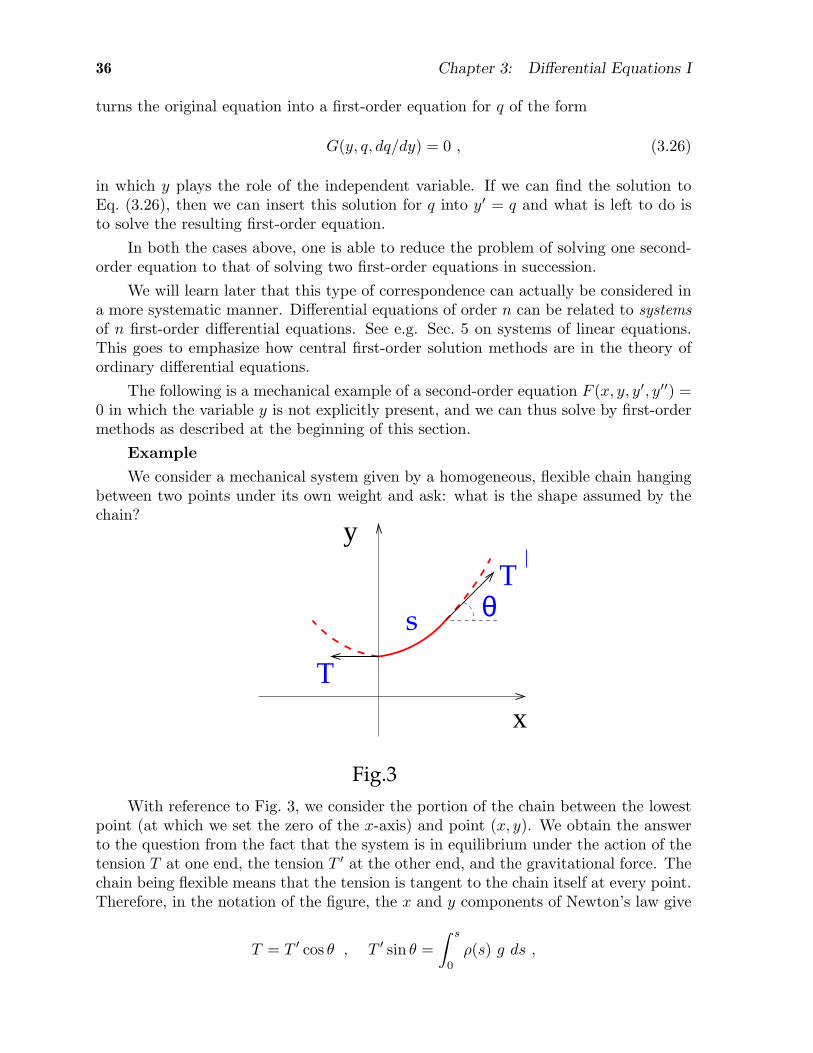
We consider a mechanical system given by a homogeneous, flexible chain hangingbetween two points under its own weight and ask: what is the shape assumed by thechain?

Fig.3

x

y

T

θT

s

With reference to Fig. 3, we consider the portion of the chain between the lowestpoint (at which we set the zero of the x-axis) and point (x, y). We obtain the answerto the question from the fact that the system is in equilibrium under the action of thetension T at one end, the tension T ′ at the other end, and the gravitational force. Thechain being flexible means that the tension is tangent to the chain itself at every point.Therefore, in the notation of the figure, the x and y components of Newton’s law give

T = T ′ cos θ , T ′ sin θ =

∫ s

0

ρ(s) g ds ,

3.8 Applications of solution methods for first-order ODEs to higher order equations37

where g is the gravitational acceleration, s is the arc length and ρ(s) is the linear massdensity of the chain. We thus have

∫ s

0

ρ(s) g ds =T

cos θsin θ = T tan θ = T

dy

dx= Ty′ .

Differentiating both sides with respect to x gives

Ty′′ =d

dx

∫ s

0

ρ(s) g ds = (d

ds

∫ s

0

ρ(s) g ds)ds

dx= ρ g

√1 + (y′)2 ,

where in the last step we have used that the chain is homogeneous, i.e., ρ(s) = ρ

is constant, and ds =√dx2 + dy2 = dx

√1 + (dy/dx)2. The differential equation

describing the shape y(x) of the chain is thus

y′′ = a√

1 + (y′)2 , (3.27)

wherea ≡ ρg/T .

Eq. (3.27) is a second-order equation in which the variable y does not appear explicitly.We proceed as described at the beginning of this section. On setting y′ = q, and theny′′ = dq/dx = q′, Eq. (3.27) reduces to the first-order nonlinear equation

q′ = a√1 + q2 ,

which can be solved by separation of variables,

∫dq

1√1 + q2

=

∫a dx .

Using that q = dy/dx = 0 at x = 0, we get

ln(q +√1 + q2) = ax ,

and, solving for q,

q =dy

dx=eax − e−ax

2.

Thus

y(x) =1

a

eax + e−ax

2+ constant =

1

acosh ax+ constant . (3.28)

The solution (3.28) gives the shape assumed by the homogeneous flexible chain. Thiscurve is called a catenary. Catenaries arise in several problems in mechanics andgeometry.

38 Chapter 4: Differential Equations II: Second-order linear ODEs

4 Differential Equations II: Second-order linearODEs

The general second-order linear equation can be written in the form

d2f

dx2+ p(x)

df

dx+ q(x)f = h(x). (4.1)

We can start by asking: Is there an integrating factor? Suppose ∃ I(x) s.t.d2If

dx2= Ih. Then

2dI

dx= Ip and

d2I

dx2= Iq. (4.2)

These equations are unfortunately incompatible in most cases. Thus, unlike the caseof first-order linear ODEs, we cannot count on there being an integrating factor.

Sec. 4.1 is devoted to discussing the general structure of solutions in the secondorder case. We give the general solution in Subsec. 4.1.1 in terms of a sum of twocontributions, the complementary function and the particular integral, and focus onthe notion of linearly independent solutions in Subsec. 4.1.2. In Subsec. 4.1.3 we observethat, although we cannot count on an integrating factor to find the general solutionfor second-order equations, we can nevertheless use the integrating factor technique ifone particular solution of the homogeneous equation is known.

In the special case in which the coefficients p(x) and q(x) in Eq. (4.1) are constants,there exist general methods to solve the equation. Second-order linear ODEs withconstant coefficients arise in many physical situations and so their solution is of greatpractical importance. We focus on such class of equations in Sec. 4.2 and Sec. 4.3,where we address respectively the question of finding the complementary function andthe question of finding the particular integral. In Sec. 4.4 we give a physical applicationof these results by considering a forced, damped oscillator.

4.1 Generalities on second-order linear equations

4.1.1 Structure of the general solution

According to the discussion of Sec. 3.3, the general solution f of Eq. (4.1) is thesum of a particular solution f0 (the “particular integral”, PI) and the general solutionf1 of the associated homogeneous equation (the “complementary function”, CF):

f = f0 + f1 , (4.3)

i.e., general solution = PI + CF . (4.4)

The associated homogeneous equation is defined by setting h(x) to zero in Eq. (4.1),

d2f

dx2+ p(x)

df

dx+ q(x)f = 0. (4.5)

4.1 Generalities on second-order linear equations 39

We have also seen in Sec. 3.2 that linearity implies the principle of superposition,namely, if u1 and u2 are two solutions of the linear homogeneous equation (4.5) thenany linear combination of them αu1 + βu2 is also solution. A converse of this alsoapplies (see Subsec. 4.1.2 for proof of this statement), in the sense that any solution ofEq. (4.5) can be expressed as a linear combination of two fundamental solutions, where“fundamental” means two linearly independent solutions according to the followingdefinition.

Two functions u1(x) and u2(x) are linearly independent if

the relation αu1(x) + βu2(x) = 0 implies α = β = 0.

This means that, if u1 and u2 are two linearly independent solutions of Eq. (4.5),the complementary function CF in Eq. (4.4) can be written in general as

CF = c1u1(x) + c2u2(x) , (4.6)

where c1 and c2 are arbitrary constants. That is, as c1 and c2 vary, all solutionsof Eq. (4.5) precisely span the whole set of linear combinations of two independentfunctions u1 and u2. We see the proof of Eq. (4.6) in the next Subsec. 4.1.2.

Example 4.1

Verify the following statement: The functions u1(x) = sinx and u2(x) = cosx arelinearly independent on the interval [0, 2π].

Answer. According to the definition given above, let us write

α sinx+ β cosx = 0 . (4.7)

One can verify the statement above by noting that there are no two constants α andβ, other than α = β = 0, such that the expression α sinx+ β cosx vanishes identicallyat every point in [0, 2π].

Alternatively, one can show this as follows. Suppose α and β exist such thatEq. (4.7) is verified. Differentiating Eq. (4.7) gives

α cosx− β sinx = 0 .

Therefore

α = βsinx

cosx⇒ β

(sin2 x

cosx+ cosx

)= 0 ⇒ β

1

cosx= 0 ⇒ β = 0 .

Thus α = β = 0.

4.1.2 Linearly independent solutions

In this section we show how the result in Eq. (4.6) arises. To this end, it is con-venient to characterize in general linearly independent functions as follows. Considertwo functions u1(x) and u2(x), and let

αu1(x) + βu2(x) = 0 . (4.8)


By differentiation Eq. (4.8) implies

αu′1(x) + βu′2(x) = 0 . (4.9)

If the determinant of the system of equations (4.8), (4.9) in α and β is nonzero, i.e.,

W (u1, u2) =

∣∣∣∣u1 u2u′1 u′2

∣∣∣∣ = u1u′2 − u2u

′1 6= 0 , (4.10)

then α = β = 0, and the functions u1 and u2 are linearly independent.

If on the other hand the determinant W (u1, u2) in Eq. (4.10) vanishes, then

u1u′2 − u2u

′1 = 0 ,

which can be integrated to give

u2 = constant × u1 .

This implies that Eq. (4.8) can be satisfied with α and β not all zero, and therefore u1and u2 are not linearly independent.

The determinant W (u1, u2) is called wronskian determinant of functions u1 and u2.

Example 4.2

The wronskian determinant of the functions u1(x) = sinx and u2(x) = cosx isgiven by

W (u1, u2) = u1u′2 − u2u

′1 = − sin2 x− cos2 x = −1 ,

which says that sinx and cosx are linearly independent (as we know from directcalculation in Example 4.1).

We are now in a position to see that the general solution of Eq. (4.5) can be writtenin the form of Eq. (4.6). Let us suppose that we have a solution u of Eq. (4.5), andlet us verify that it can be expressed as a linear combination of linearly independentsolutions u1 and u2. Since u, u1 and u2 all solve Eq. (4.5), with nonzero coefficients ofthe second-derivative, first-derivative and no-derivative terms, we must have vanishingdeterminant ∣∣∣∣∣∣

u u1 u2u′ u′1 u′2u′′ u′′1 u′′2

∣∣∣∣∣∣= 0 . (4.11)

Analogously to Eq. (4.10) for the case of two functions, Eq. (4.11) gives the wronskiandeterminant for three functions, and its vanishing for the three solutions u, u1 and u2implies that

αu+ βu1 + γu2 = 0 (4.12)

is satisfied with α, β and γ not all zero. If α was zero, β and γ nonzero wouldcontradict the linear independence of u1 and u2, so α 6= 0. Then if u is nontrivial βand γ cannot both be zero. Thus, solving Eq. (4.12) for u expresses the solution u asa linear combination of u1 and u2.

4.2 2nd-order linear ODE’s with constant coefficients: The Complementary Function 41

Example 4.3

The general solution of the 2nd-order linear ODE

y′′ + y = 0 (4.13)

is

A sinx+B cosx . (4.14)

To show this, it is sufficient to show that i) sinx and cosx solve the equation (forinstance, by direct computation) and ii) sinx and cosx are linearly independent (asdone by two methods in Example 4.1 and in Example 4.2). Then the result in Eq. (4.6)guarantees that the general solution has the form (4.14).

4.1.3 An application of the integrating factor technique: finding the

general solution once one solution of the homogeneous equation is known

This subsection illustrates that, if one particular solution of the homogeneousequation is known, then one can find the general solution by applying the integratingfactor technique.

Suppose we have a solution u of the homogeneous equation:

d2u

dx2+ p(x)

du

dx+ q(x)u = 0, (4.15)

Then write f = uv and u′ ≡ du

dxetc. so that

f ′ = u′v + uv′ ; f ′′ = u′′v + 2u′v′ + uv′′. (4.16)

Substituting these results into (4.1) we obtain

h = f ′′ + pf ′ + qf

= u′′v + 2u′v′ + uv′′ + pu′v + puv′ + quv

= v(u′′ + pu′ + qu) + uv′′ + 2u′v′ + puv′

= 0 + uv′′ + 2u′v′ + puv′.

(4.17)

Now define w ≡ v′ and find

uw′ + (2u′ + pu)w = h ⇒

IF = exp

[ ∫ (2u′

u+ p)dx

]

= u2e∫p dx.

(4.18)

Finally can integrate

v′(x) = w(x) = u−2(x)e−∫

x

p dx∫ x

x0

e∫

x′

p dxhu dx′. (4.19)

Thus if we can find one solution, u, of any second-order linear equation, we can findthe general solution f(x) = αu(x) + u(x)v(x, x0).


4.2 2nd-order linear ODE’s with constant coefficients: TheComplementary Function

Suppose the coefficients of the unknown function f and its derivatives are mereconstants:

Lf = a2d2f

dx2+ a1

df

dx+ a0f = h(x). (4.20)

In this case there exist general methods of solution. The solution proceeds through acombination of the complementary function and the particular integral. In this sectionwe deal with the complementary function. In Sec. 4.3 we deal with the particularintegral.

4.2.1 Auxiliary equation

We look for a complementary function y(x) that satisfies Ly = 0. We try y = eαx.Substituting this into a2y

′′ + a1y′ + a0y = 0 we find that the equation is satisfied ∀x

provideda2α

2 + a1α+ a0 = 0. (4.21)

This condition for the exponent α is called the auxiliary equation. It has two roots

α± ≡ −a1 ±√a21 − 4a2a02a2

, (4.22)

so the CF isy = A+e

α+x +A−eα−x. (4.23)

Example 4.4Solve

d2y

dx2+ 4

dy

dx+ 3y = 0.

The auxiliary equation is (α+ 3)(α+ 1) = 0, so the CF is y = Ae−3x +Be−x.

Example 4.5Solve

Ly =d2y

dx2− 2

dy

dx+ 5y = 0.

The auxiliary equation is α = 12 (2±

√4− 20) = 1±2i, so y = Ae(1+2i)x+Be(1−2i)x.

But this is complex!

However, L is real operator. So 0 = ℜe(Ly) = L[ℜe(y)] and ℜe(y) is also a solution.Ditto ℑm(y). Consequently the solution can be written

y = ex[A′ cos(2x) +B′ sin(2x)

].

Example 4.6Find the solutions to the equation of Example 4.5 for which y(0) = 1 and(dy/dx)0 = 0.

4.3 2nd-order linear ODE’s with constant coefficients: The Particular Integral 43

Solution: We obtain simultaneous equations for A′ and B′ by evaluating thegeneral solution and its derivative at x = 0:

1 = A′

0 = A′ + 2B′ ⇒ B′ = − 12 ⇒ y = ex

[cos(2x)− 1

2 sin(2x)].

4.2.2 Factorization of operators & repeated roots

The auxiliary equation (4.21) is just the differential equation Lf = 0 with d/dxreplaced by α. So just as the roots of a polynomial enables us to express the polynomialas a product of terms linear in the variable, so the knowledge of the roots of the auxiliaryequation allows us to express L as a product of two first-order differential operators:

( d

dx− α−

)( d

dx− α+

)f =

d2f

dx2− (α− + α+)

df

dx+ α−α+f

=d2f

dx2+a1a2

df

dx+a0a2

≡ Lf

a2,

(4.24)

where we have used our formulae (2.25) for the sum and product of the roots of apolynomial. The CF is made up of exponentials because

( d

dx− α−

)eα−x = 0 ;

( d

dx− α+

)eα+x = 0.

What happens if a21 − 4a2a0 = 0? Then α− = α+ = α and

Lf =( d

dx− α

)( d

dx− α

)f. (4.25)

It follows that

L(xeαx

)=( d

dx− α

)( d

dx− α

)xeαx

=( d

dx− α

)eαx = 0,

and the CF is y = Aeαx +Bxeαx.

Example 4.7Solve

d2y

dx2− 2

dy

dx+ y = 0.

The auxiliary equation is (α− 1)2 = 0, so y = Aex +Bxex.

4.2.3 Extension to higher orders

These results we have just derived generalize easily to linear equations with con-stant coeffs of any order.

Example 4.8Solve

d4y

dx4− 2

d3y

dx3+ 2

d2y

dx2− 2

dy

dx+ y = 0.

The auxiliary equation is (α− 1)2(α− i)(α+ i) = 0, so

y = ex(A+Bx) + C cosx+D sinx.


4.3 2nd-order linear ODE’s with constant coefficients: TheParticular Integral

Recall that the general solution of Lf = h is CF+f0 where the particular integralf0 is any function for which Lf0 = h. There is a general technique for finding PIs. Thistechnique, which centres on Green’s functions, lies beyond the syllabus although itis outlined in Chapter 6. For simple inhomogeneous part h we can get by with the useof trial functions. The type of function to be tried depends on the nature of h.

4.3.1 Polynomial h Suppose h is a sum of some powers of x,

h(x) = b0 + b1x+ b2x2 + · · · (4.26)

Then we tryf(x) = c0 + c1x+ c2x

2 + · · ·⇒ f ′ = c1 + 2c2x+ · · ·

f ′′ = 2c2 + · · ·(4.27)

soh(x) = a2f

′′ + a1f′ + a0f =(a0c0 + a1c1 + a22c2 + · · ·)

+ (a0c1 + a12c2 + · · ·)x+ (a0c2 + · · ·)x2+ · · ·

(4.28)

Comparing powers of x0, x1, . . . on the two sides of this equation, we obtained coupledlinear equations for the cr in terms of the br. We solve these equations from the bottomup; e.g. for quadratic h

c2 =b2a0,

c1 =b1 − 2a1c2

a0,

c0 =b0 − a1c1 − 2a2c2

a0.

(4.29)

Notice that the procedure doesn’t work if a0 = 0; the orders of the polynomials on leftand right then inevitably disagree. This difficulty may be resolved by recognizing thatthe equation is then a first-order one for g ≡ f ′ and using a trial solution for g thatcontains a term in x2.

Example 4.9Find the PI for

f ′′ + 2f ′ + f = 1 + 2x+ 3x2.

Try f = c0 + c1x+ c2x2; have

x2 :

x1 :

x0 :

c2 = 3

4c2 + c1 = 2

2c2 + 2c1 + c0 = 1

⇒ c1 = 2(1− 2c2) = −10

c0 = 1− 2(c2 + c1) = 1− 2(3− 10) = 15


Checkf = 15− 10x+ 3x2,

2f ′ = (−10 + 6x)× 2,

f ′′ = 6,

L(f) = 1 + 2x+ 3x2.

4.3.2 Exponential f When h = Heγx, we try f = P eγx. Substituting this into thegeneral second-order equation with constant coefficients we obtain

P (a2γ2 + a1γ + a0)e

γx = Heγx. (4.30)

Cancelling the exponentials, solving for P , and substituting the result into f = P eγx,we have finally

f =Heγx

a2γ2 + a1γ + a0

=Heγx

a2(γ − α−)(γ − α+)where CF = A±e

α±x.

(4.31)


f ′′ + 3f ′ + 2f = e2x.

So the PI is f =e2x

4 + 6 + 2= 1

12e2x.

If h contains two or more exponentials, we find separate PIs for each of them, andthen add our results to get the overall PI.


f ′′ + 3f ′ + 2f = e2x + 2ex.

Reasoning as above we conclude that f1 ≡ 112e

2x satisfies f ′′1 + 3f ′1 + 2f1 = e2x.

and f2 ≡ 2ex

1 + 3 + 2= 1

3ex satisfies f ′′2 + 3f ′2 + 2f2 = ex,

so 112e

2x + 13ex satisfies the given equation.

From equation (4.31) it is clear that we have problem when part of h is in theCF because then one of the denominators of our PI vanishes. The problem we have toaddress is the solution of

Lf = a2

( d

dx− α1

)( d

dx− α2

)f = Heα2x. (4.32)

P eα2x is not a useful trial function for the PI because Leα2x = 0. Instead we tryPxeα2x. We have ( d

dx− α2

)Pxeα2x = P eα2x, (4.33)


and

L(Pxeα2x

)= a2

( d

dx− α1

)P eα2x = a2P (α2 − α1)e

α2x. (4.34)

Hence, we can solve for P so long as α2 6= α1: P =H

a2(α2 − α1).


f ′′ + 3f ′ + 2f = e−x.

The CF is Ae−2x +Be−x, so we try f = Pxe−x. We require

e−x =( d

dx+ 2)( d

dx+ 1)Pxe−x =

( d

dx+ 2)P e−x

= P e−x.

Thus P = 1 and f = xe−x.

What if α1 = α2 = α and h = Heαx? Then we try f = Px2eαx:

Heαx = a2

( d

dx− α

)2Px2eαx = a2

( d

dx− α

)2Pxeαx

= 2a2P eαx ⇒ P =

H

2a2

4.3.3 Sinusoidal h

Suppose h = H cosx, so Lf ≡ a2f′′ + a1f

′ + a0f = H cosx.

Clumsy method:f = A cosx+B sinx

. . . . . .

Elegant method: Find solutions z(x) of the complex equation

Lz = Heix. (4.35)

Since L is real

ℜe(Lz) = L[ℜe(z)] = ℜe(Heix) = Hℜe(eix) = H cosx, (4.36)

so the real part of our solution z will answer the given problem.

Set z = P eix (P complex)

Lz = (−a2 + ia1 + a0)P eix ⇒ P =

H

−a2 + ia1 + a0. (4.37)

Finally,

f = Hℜe

( eix

(a0 − a2) + ia1

)

= H(a0 − a2) cosx+ a1 sinx

(a0 − a2)2 + a21.

(4.38)


Note:

We shall see below that in many physical problems explicit extraction of the realpart is unhelpful; more physical insight can be obtained from the first than thesecond of equations (4.38). But don’t forget that ℜe operator! It’s especiallyimportant to include it when evaluating the arbitrary constants in the CF byimposing initial conditions.


f ′′ + 3f ′ + 2f = cosx.

We actually solve

z′′ + 3z′ + 2z = eix.

Hence

z = P eix where P =1

−1 + 3i + 2.

Extracting the real part we have finally

f = ℜe

( eix

1 + 3i

)= 1

10 (cosx+ 3 sinx).

What do we do if h = H sinx? We solve Lz = Heix and take imaginary parts ofboth sides.


f ′′ + 3f ′ + 2f = sinx.

Solving z′′ + 3z′ + 2z = eix with z = P eix we have

P =1

1 + 3i⇒ f = ℑm

( eix

1 + 3i

)= 1

10 (sinx− 3 cosx).

Note:

It is often useful to express A cos θ+B sin θ as A cos(θ+φ). We do this by notingthat cos(θ + φ) = cosφ cos θ − sinφ sin θ, so

A cos θ +B sin θ =√A2 +B2

( A√A2 +B2

cos θ +B√

A2 +B2sin θ

)

=√A2 +B2 cos(θ + φ),

where cosφ = A/√A2 +B2 and sinφ = −B/

√A2 +B2.



f ′′ + 3f ′ + 2f = 3 cosx+ 4 sinx.

The right-hand side can be rewritten 5 cos(x + φ) = 5ℜe(ei(x+φ)), where φ =arctan(−4/3). So our trial solution of the underlying complex equation is z =P ei(x+φ). Plugging this into the equation, we find

P =5

−1 + 3i + 2=

5

1 + 3i,

so the required PI is

f0 = 5ℜe

(ei(x+φ)1 + 3i

)= 1

2

[cos(x+ φ) + 3 sin(x+ φ)

].

The last three examples are rather easy because eix does not occur in the CF(which is Ae−x +Be−2x). What if eix is in the CF? Then we try z = Pxeix.


f ′′ + f = cosx ⇒ z′′ + z = eix

From the auxiliary equation we find that the equation can be written( d

dx+ i)( d

dx− i)z = eix.

For the PI Pxeix we require

eix =( d

dx+ i)( d

dx− i)Pxeix =

( d

dx+ i)P eix = 2iP eix

⇒ P =1

2i⇒ f = ℜe

(xeix2i

)= 1

2x sinx

4.3.4 Exponentially decaying sinusoidal h Since we are handling sinusoids by express-ing them in terms of exponentials, essentially nothing changes if we are confronted bya combination of an exponential and sinusoids:


f ′′ + f = e−x(3 cosx+ 4 sinx

).

The right-hand side can be rewritten 5e−x cos(x + φ) = 5ℜe(e(i−1)x+iφ), whereφ = arctan(−4/3). So our trial solution of the underlying complex equation isz = P e(i−1)x+iφ. Plugging this into the equation, we find

P =5

(i− 1)2 + 1=

5

1− 2i.

Finally the required PI is

f0 = 5ℜe

(e(i−1)x+iφ

1− 2i

)= e−x

[cos(x+ φ)− 2 sin(x+ φ)

].

4.4 Application to Oscillators 49

4.4 Application to Oscillators

Second-order differential equations with constant coefficients arise from all sorts ofphysical systems in which something undergoes small oscillations about a point ofequilibrium. It is hard to exaggerate the importance for physics of such systems.Obvious examples include the escapement spring of a watch, the horn of a loudspeakerand an irritating bit of trim that makes a noise at certain speeds in the car. Lessfamiliar examples include the various fields that the vacuum sports, which include theelectromagnetic field and the fields whose excitations we call electrons and quarks.

The equation of motion of a mass that oscillates in response to a periodic drivingforce mF cosωt is

mx = − mω20x − mγx + mF cosωt.

spring friction forcing(4.39)

Gathering the homogeneous and inhomogeneous terms onto the left- and right-handsides, respectively, we see that the associated complex equation is

z + γz + ω20z = F eiωt. (4.40)

4.4.1 Transients The auxiliary equation of (4.40) is

α2 + γα+ ω20 = 0 ⇒ α = − 1

2γ ± i√ω20 − 1

4γ2

= − 12γ ± iωγ where ωγ ≡ ω0

√1− 1

4γ2/ω2

0 .

Here we concentrate on the case that ω20− 1

4γ2 > 0 which corresponds to the case there

are oscillating solutions. Using the solutions for α we may determine the CF

x = e−γt/2[A cos(ωγt) +B sin(ωγt)

]= e−γt/2A cos(ωγt+ ψ), (4.41)

where ψ, the phase angle, is an arbitrary constant. Since γ > 0, we have that theCF → 0 as t → ∞. Consequently, the part of motion that is described by the CF iscalled the transient response.

4.4.2 Steady-state solutions The PI of equation (4.40) is

x = ℜe

( F eiωt

ω20 − ω2 + iωγ

). (4.42)

The PI describes the steady-state response that remains after the transient has diedaway.

In (4.42) the bottom =√(ω2

0 − ω2)2 + ω2γ2 eiφ, where φ ≡ arctan( ωγ

ω20 − ω2

), so

the PI may also be written

x =Fℜe

(ei(ωt−φ)

)√

(ω20 − ω2)2 + ω2γ2

=F cos(ωt− φ)√

(ω20 − ω2)2 + ω2γ2

. (4.43)


Amplitude and phase of adriven oscillator. Full lines arefor γ = 0.1ω0, dashed lines forγ = 0.5ω0.

For φ > 0, x achieves the same phase as F at t greater by φ/ω, so φ is called the phaselag of the response.

The amplitude of the response is

A =F√

(ω20 − ω2)2 + ω2γ2

, (4.44)

which peaks when

0 =dA−2

dω∝ −4(ω2

0 − ω2)ω + 2ωγ2 ⇒ ω2 = ω20 − 1

2γ2. (4.45)

ωR ≡√ω20 − γ2/2 is called the resonant frequency. Note that the frictional coefficient

γ causes ωR to be smaller than the natural frequency ω0 of the undamped oscillator.

The figure shows that the amplitude of the steady-state response becomes verylarge at ω = ωR if γ/ω0 is small. The figure also shows that the phase lag of theresponse increases from small values at ω < ωR to π at high frequencies. Manyimportant physical processes, including dispersion of light in glass, depend on thisoften rapid change in phase with frequency.

4.4 Application to Oscillators 51

4.4.3 Power input Power in is W = F x, where F = mF cosωt. Since ℜe(z1) ×ℜe(z2) 6= ℜe(z1z2), we have to extract real bits before multiplying them together

W = F x = ℜe(mF eiωt)× ℜe(iωF ei(ωt−φ)

)√

(ω20 − ω2)2 + ω2γ2

=ωmF 2

√(ω2

0 − ω2)2 + ω2γ2[− cos(ωt) sin(ωt− φ)]

= −12ωmF

2

√(ω2

0 − ω2)2 + ω2γ2[sin(2ωt− φ) + sin(−φ)].

(4.46)

Averaging over an integral number of periods, the mean power is

W =12ωmF

2 sinφ√(ω2

0 − ω2)2 + ω2γ2. (4.47)

4.4.4 Energy dissipated Let’s check that the mean power input is equal to the rate ofdissipation of energy by friction. The dissipation rate is

D = mγxx =mγω2F 2 1

2

(ω20 − ω2)2 + ω2γ2

. (4.48)

It is equal to work done because sinφ = γω/√(ω2

0 − ω2)2 + ω2γ2.

4.4.5 Quality factor Now consider the energy content of the transient motion thatthe CF describes. By (4.41) its energy is

E = 12 (mx

2 +mω20x

2)

= 12mA

2e−γt[14γ

2 cos2 η + ωγγ cos η sin η + ω2γ sin

2 η + ω20 cos

2 η]

(η ≡ ωγt+ ψ)(4.49)

For small γ/ω0 this becomes

E ≃ 12m(ω0A)

2e−γt. (4.50)

We define the quality factor Q to be

Q ≡ E(t)

E(t− π/ω0)− E(t+ π/ω0)≃ 1

eπγ/ω0 − e−πγ/ω0= 1

2 csch(πγ/ω0)

≃ ω0

2πγ(for small γ/ω0).

(4.51)

Q is the inverse of the fraction of the oscillator’s energy that is dissipated in one period.It is approximately equal to the number of oscillations conducted before the energydecays by a factor of e.

52 Chapter 5: Systems of linear differential equations

5 Systems of linear differential equations

Many physical systems require more than one variable to quantify their configuration:for instance an electric circuit might have two connected current loops, so one needsto know what current is flowing in each loop at each moment. A set of differentialequations – one for each variable – will determine the dynamics of such a system.

For example, a system of first-order differential equations in the n variables

y1(x), y2(x), . . . , yn(x) (5.1)

will have the general form

y′1 = F1(x, y1, y2, . . . , yn)

y′2 = F2(x, y1, y2, . . . , yn)

· · ·

y′n = Fn(x, y1, y2, . . . , yn) (5.2)

for given functions F1, . . ., Fn.

Observe also that in general an nth-order differential equation

y(n) = G(x, y, y′, y′′, . . . , y(n−1)) (5.3)

can be thought of as a system of n first-order equations. To see this, set new variablesy1 = y; y2 = y′; . . . ; yn = y(n−1). Then the system of first-order equations

y′1 = y2

· · ·

y′n−1 = yn

y′n = G(x, y1, y2, . . . , yn) (5.4)

is equivalent to the starting nth-order equation.

If we have a system of differential equations which are linear and have constantcoefficients, the procedure for solving them is an extension of the procedure for solvinga single linear differential equation with constant coefficients. In Subsec. 5.1 we discussthis case and illustrate the solution methods. In Subsec. 5.2 we consider applicationsto linear electrical circuits.

5.1 Systems of linear ODE’s with constant coefficients 53

5.1 Systems of linear ODE’s with constant coefficients

Systems of linear ODEs with constant coefficients can be solved by a generalizationof the method seen for single ODE by writing the general solution as

General solution = PI + CF ,

where the complementary function CF will be obtained by solving a system of auxiliary

equations, and the particular integral PI will be obtained from a set of trial functions

with functional form as the inhomogeneous terms.

The steps for treating a system of linear differential equations with constant coef-ficients are:

1. Arrange the equations so that terms on the left are all proportional to an unknownvariable, and already known terms are on the right.

2. Find the general solution of the equations that are obtained by setting the rightsides to zero. The result of this operation is the CF. It is usually found by replacingthe unknown variables by multiples of eαt (if t is the independent variable) andsolving the resulting algebraic equations.

3. Find a particular integral by putting in a trial solution for each term – polynomial,exponential, etc. – on the right hand side.

This is best illustrated by some examples.

Example 5.1Solve

dx

dt+

dy

dt+ y = t,

−dy

dt+ 3x+ 7y = e2t − 1.

It is helpful to introduce the shorthand

L

(xy

)=

dx

dt+dy

dt+ y

3x −dy

dt+ 7y

.

To find CF

Set

(xy

)=

(Xeαt

Y eαt

)α,X, Y complex nos to be determined

Plug into L

(xy

)= 0 and cancel the factor eαt

αX + (α+ 1)Y = 0,

3X + (7− α)Y = 0.(5.5)


The theory of equations, to be discussed early next term, shows that these equa-tions allow X,Y to be non-zero only if the determinant

∣∣∣∣α α+ 13 7− α

∣∣∣∣ = 0,

which in turn implies that α(7 − α) − 3(α + 1) = 0 ⇒ α = 3, α = 1. Wecan arrive at the same conclusion less quickly by using the second equation toeliminate Y from the first equation. So the bottom line is that α = 3, 1 are theonly two viable values of α. For each value of α either of equations (5.5) imposesa ratio∗ X/Y

α = 3 ⇒ 3X + 4Y = 0 ⇒ Y = − 34X,

α = 1 ⇒ X + 2Y = 0 ⇒ Y = − 12X.

Hence the CF made up of

(xy

)= Xa

(1− 3

4

)e3t and

(xy

)= Xb

(1− 1

2

)et.

The two arbitrary constants in this CF reflect the fact that the original equationswere first-order in two variables.

To find PI

(i) Polynomial part

Try

(xy

)=

(X0 +X1tY0 + Y1t

)

Plug into L

(xy

)=

(t−1

)

X1 + Y1 + Y1t+ Y0 = t 3(X0 +X1t)− Y1 + 7(Y0 + Y1t) = −1⇓ ⇓

Y1 = 1; X1 + Y1 + Y0 = 0 3X0 + 7Y0 = 0; 3X1 + 7Y1 = 0⇓ ⇓

X1 + Y0 = −1 X1 = − 73

Consequently, Y0 = −1 + 73 = 4

3 and X0 = − 73Y0 = − 28

9

Thus (xy

)=

(− 28

9 − 73 t

43 + t

)

(ii) Exponential part

Try

(xy

)=

(XY

)e2t

∗ The allowed values of α are precisely those for which you get the same value of X/Y from

both of equations (5.5).

5.1 Systems of linear ODE’s with constant coefficients 55

Plug into L

(xy

)=

(0e2t

)and find

2X + (2 + 1)Y = 0 ⇒ X = − 32Y

3X + (−2 + 7)Y = 1 ⇒ (− 92 + 5)Y = 1

Hence Y = 2, X = −3.

Putting everything together the general solution is(xy

)= Xa

(1− 3

4

)e3t +Xb

(1− 1

2

)et +

(−32

)e2t +

(− 28

9 − 73 t

43 + t

)(5.6)

We can use the arbitrary constants in the above solution to obtain a solution inwhich x and y or x and y take on any prescribed values at t = 0:

Example 5.2For the differential equations of Example 5.1, find the solution in which

x(0) = − 193

y(0) = 3

Solution: Evaluate the time derivative of the GS at t = 0 and set the result equalto the given data:

(− 19

33

)= 3Xa

(1− 3

4

)+Xb

(1− 1

2

)+ 2

(−32

)+

(− 7

31

)

Hence

3Xa +Xb = 2

− 94Xa − 1

2Xb = −2⇒

Xa =−2

−3/2= 4

3

Xb = 2− 3Xa = −2

Here’s another, more complicated example.

Example 5.3Solve

d2x

dt2+

dy

dt+ 2x = 2 sin t+ 3 cos t+ 5e−t

dx

dt+

d2y

dt2− y = 3 cos t− 5 sin t− e−t

givenx(0) = 2; y(0) = −3

x(0) = 0; y(0) = 4

To find CF

Set x = Xeαt, y = Y eαt

⇒ (α2 + 2)X + αYαX + (α2 − 1)Y

= 0 ⇒ α4 = 2

⇒ α2 = ±√2 ⇒ α = ±β, ±iβ (β ≡ 21/4)


and Y/X = −(α2 + 2)/α so the CF is

(xy

)= Xa

(β

2 +√2

)e−βt +Xb

(−β

2 +√2

)eβt

+Xc

(iβ

2−√2

)e−iβt +Xd

(−iβ

2−√2

)eiβt

Notice that the functions multiplying Xc and Xd are complex conjugates of oneanother. So if the solution is to be real Xd has to be the complex conjugate ofXc and these two complex coefficients contain only two real arbitrary constantsbetween them. There are four arbitrary constants in the CF because we are solvingsecond-order equations in two dependent variables.

To Find PI

Set (x, y) = (X,Y )e−t ⇒

X − Y + 2X = 5

−X + Y − Y =− 1⇒ X = 1

Y = −2⇒

(xy

)=

(1−2

)e−t

Have 2 sin t+ 3 cos t = ℜe(√13ei(t+φ)), where cosφ = 3/

√13, sinφ = −2/

√13.

Similarly 3 cos t− 5 sin t = ℜe(√34ei(t+ψ)), where cosψ = 3/

√34, sinψ = 5/

√34

Set (x, y) = ℜe[(X,Y )eit] and require

−X + iY + 2X = X + iY =√13eiφ

iX − Y − Y = iX − 2Y =√34eiψ

⇒−iY =

√13eiφ + i

√34eiψ

iX = 2i√13eiφ −

√34eiψ

sox = ℜe(2

√13ei(t+φ) + i

√34ei(t+ψ))

= 2√13(cosφ cos t− sinφ sin t)−

√34(sinψ cos t+ cosψ sin t)

= 2[3 cos t+ 2 sin t]− 5 cos t− 3 sin t

= cos t+ sin t

Similarly

y = ℜe(√13iei(t+φ) −

√34ei(t+ψ))

=√13(− sinφ cos t− cosφ sin t)−

√34(cosψ cos t− sinψ sin t)

= 2 cos t− 3 sin t− 3 cos t+ 5 sin t

= − cos t+ 2 sin t.

Thus the complete PI is

(xy

)=

(cos t+ sin t

− cos t+ 2 sin t

)+

(1−2

)e−t.

5.2 LCR circuits 57

For the initial-value problem

PI(0) =

(1−2

)+

(1−1

)=

(2−3

); PI(0) =

(−12

)+

(12

)=

(04

)

CF(0) =

(2−3

)−(

2−3

)=

(00

); CF(0) =

(04

)−(04

)=

(00

)

So the PI satisfies the initial data and Xa = Xb = Xc = Xd = 0.

In general the number of arbitrary constants in the general solution should bethe sum of the orders of the highest derivative in each variable. There are exceptionsto this rule, however, as the following example shows. This example also illustratesanother general point: that before solving the given equations, one should always tryto simplify them by adding a multiple of one equation or its derivative to the other.

Example 5.4Solve

dx

dt+

dy

dt+ y = t,

d2x

dt2+

d2y

dt2+ 3x+ 7y = e2t.

(5.7)

We differentiate the first equation and substract the result from the second. Thenthe system becomes first-order – in fact the system solved in Example 5.1. From(5.6) we see that the general solution contains only two arbitrary constants ratherthan the four we might have expected from a cursory glance at (5.7). To under-stand this phenomenon better, rewrite the equations in terms of z ≡ x + y asz + z − x = t and z + 7z − 4x = e2t. The first equation can be used to make x afunction x(z, z, t). Using this to eliminate x from the second equation we obtainan expression for z(z, z, t). From this expression and its derivatives w.r.t. t we canconstruct a Taylor series for z once we are told z(t0) and z(t0). Hence the generalsolution should have just two arbitrary constants.

5.2 LCR circuits

The dynamics of a linear electrical circuit is governed by a system of linear equa-tions with constant coefficients. These may be solved by the general technique de-scribed in the previous section. In many cases they may be more easily solved byjudicious addition and subtraction along the lines illustrated in Example 5.4.

Example 5.5Consider the electrical circuit pictured in the figure.


Using Kirchhoff’s laws

RI1 +Q

C+ L

dI1dt

= E1

LdI2dt

+RI2 −Q

C= 0.

(5.8)

We first differentiate to eliminate Q

d2I1dt2

+R

L

dI1dt

+1

LC(I1 − I2) = 0

d2I2dt2

+R

L

dI2dt

− 1

LC(I1 − I2) = 0.

(5.9)

We now add the equations to obtain

d2S

dt2+R

L

dS

dt= 0 where S ≡ I1 + I2. (5.10)

Subtracting the equations we find

d2D

dt2+R

L

dD

dt+

2

LCD = 0 where D ≡ I1 − I2. (5.11)

We now have two uncoupled second-order equations, one for S and one for D. We cansolve each in the standard way (Section 4.2).

Example 5.6Determine the time evolution of the LCR circuit in Example 5.5.

Solution.

The auxiliary equation for (5.10) is α2 +Rα/L = 0, and its roots are

α = 0 ⇒ S = constant and α = −R/L ⇒ S ∝ e−Rt/L. (5.12)

Since the right side of (5.10) is zero, no PI is required.

5.2 LCR circuits 59

The auxiliary equation for (5.11) is

α2 +R

Lα+

2

LC= 0 ⇒ α = − 1

2

R

L± i√

LC

√2− 1

4CR2/L = − 1

2

R

L± iωR. (5.13)

Again no PI is required.

Adding the results of (5.12) and (5.13), the general solutions to (5.10) and (5.11)are

I1 + I2 = S = S0 + S1e−Rt/L ; I1 − I2 = D = D0e

−Rt/2L sin(ωRt+ φ).

From the original equations (5.9) it is easy to see that the steady-state currents areI1 = I2 = 1

2S0 = 12E1/R. Hence, the final general solution is

I1 + I2 = S(t) = Ke−Rt/L +E1

R

I1 − I2 = D(t) = D0e−Rt/2L sin(ωRt+ φ).

(5.14)

Example 5.7Suppose that the battery in the LCR circuit above is first connected up at t = 0.Determine I1, I2 for t > 0.

Solution: We have I1(0) = I2(0) = 0 and from the diagram we see that I1(0) =E1/L and I2 = 0. Looking at equations (5.14) we set K = −E1/R to ensurethat I1(0) + I2(0) = 0, and φ = 0 to ensure that I1(0) = I2(0). Finally we set

D0 =E1

LωRto ensure that D(0) =

E1

L.

60 Chapter 6: Green Functions

6 Green Functions∗

In this section we describe a powerful technique for generating particular integrals.We illustrate it by considering the general second-order linear equation

Lx(y) ≡ a2(x)d2y

dx2+ a1(x)

dy

dx+ a0(x)y = h(x). (6.1)

On dividing through by a2 one sees that without loss of generality we can set a2 = 1.

6.1 The Dirac δ-function

Consider series of ever bumpier functions such that∫∞−∞ f(x) dx = 1, e.g.

Define δ(x) as limit of such functions. (δ(x) itself isn’t a function really.) Then

δ(x) = 0 for x 6= 0 and

∫ ∞

−∞δ(x) dx = 1

δ’s really important property is that

∫ b

a

f(x)δ(x− x0) dx = f(x0) ∀{a < x0 < bf(x)

Exercises (1):

(i) Prove that δ(ax) = δ(x)/|a|. If x has units of length, what dimensions has δ?

(ii) Prove that δ(f(x)) =∑xkδ(x−xk)/|f ′(xk)|, where the xk are all points satisfying

f(xk) = 0.

∗ Lies beyond the syllabus

6.3 Finding Gx061

6.2 Defining the Green’s function

Now suppose for each fixed x0 we had the function Gx0(x) such that

LxGx0= δ(x− x0). (6.2)

Then we could easily obtain the desired PI:

y(x) ≡∫ ∞

−∞Gx0

(x)h(x0) dx0. (6.3)

y is the PI because

Lx(y) =

∫ ∞

−∞LxGx0

(x)h(x0) dx0

=

∫δ(x− x0)h(x0) dx0

= h(x).

Hence, once you have the Green’s function Gx0you can easily find solutions for

various h.

6.3 Finding Gx0

Let y = v1(x) and y = v2(x) be two linearly independent solutions of Lxy = 0 –i.e. let the CF of our equation be y = Av1(x) + Bv2(x). At x 6= x0, LxGx0

= 0, soGx0

= A(x0)v1(x) + B(x0)v2(x). But in general we will have different expressions forGx0

in terms of the vi for x < x0 and x > x0:

Gx0=

{A−(x0)v1(x) +B−(x0)v2(x) x < x0A+(x0)v1(x) +B+(x0)v2(x) x > x0.

(6.4)

We need to choose the four functions A±(x0) and B±(x0). We do this by:

(i) obliging Gx0to satisfy boundary conditions at x = xmin < x0 and x = xmax > x0

(e.g. limx→±∞

Gx0= 0);

(ii) ensuring LxGx0= δ(x− x0).

We deal with (i) by defining u± ≡ P±v1 + Q±v2 with P±, Q± chosen s.t. u− satisfiesgiven boundary condition at x = xmin and u+ satisfies condition at xmax. Then

Gx0(x) =

{C−(x0)u−(x) x < x0,C+(x0)u+(x) x > x0.

(6.5)

We get C± by integrating the differential equation from x0 − ǫ to x0 + ǫ:

1 =

∫ x0+ǫ

x0−ǫδ(x− x0) dx =

∫ x0+ǫ

x0−ǫLxGx0

dx

=

∫ x0+ǫ

x0−ǫ

(d2Gx0

dx2+ a1(x)

dGx0

dx+ a0(x)Gx0

(x)

)dx

=

[dGx0

dx+ a1(x0)Gx0

(x)

]x0+ǫ

x0−ǫ+

∫ x0+ǫ

x0−ǫ

(a0 −

da1dx

)Gx0

(x) dx.

(6.6)

62 Chapter 6: Green Functions

We assume that Gx0(x) is finite and continuous at x0, so the second term in [. . .]

vanishes and the remaining integral vanishes as ǫ → 0. Then we have two equationsfor C±:

1 = C+(x0)du+dx

∣∣∣∣x0

− C−(x0)du−dx

∣∣∣∣x0

0 = C+(x0)u+(x0)− C−(x0)u−(x0).

(6.7)

Solving for C± we obtain

C±(x0) =u∓∆

∣∣∣∣x0

where ∆(x0) ≡(du+dx

u− − u+du−dx

)

x0

. (6.8)

Substing these solutions back into (6.5) we have finally

Gx0(x) =

u+(x0)u−(x)

∆(x0)x < x0

u−(x0)u+(x)

∆(x0)x > x0.

(6.9)

Example 6.1Solve

Lx =d2y

dx2− k2y = h(x) subject to lim

x→±∞y = 0.

The required complementary functions are u− = ekx, u+ = e−kx, so

∆(x0) = −ke−kxekx − e−kxkekx = −2k.

Hence

Gx0(x) = − 1

2k

{e−k(x0−x) x < x0ek(x0−x) x > x0

= − 1

2ke−k|x0−x|

and

y(x) = − 1

2k

[e−kx

∫ x

−∞ekx0h(x0) dx0 + ekx

∫ ∞

x

e−kx0h(x0)

]dx0.

Suppose h(x) = cosx = ℜe(eix). Then

−2ky(x) = ℜe

(e−kx

[ex0(i+k)

i+ k

]x

−∞+ ekx

[ex0(i−k)

i− k

]∞

x

)

Soy = − cosx

1 + k2

as expected.

complex numbers and ordinary differential equations

Documents