complex algebraic geometry (notes of jean gallier from ...cis610/calg1.pdf · complex algebraic...
TRANSCRIPT

Complex Algebraic Geometry
(Notes of Jean Gallier From Math 622/623,Fall 2003– Spring 2004,Lectures by S.S. Shatz)
Jean GallierDepartment of Computer and Information Science
University of PennsylvaniaPhiladelphia, PA 19104, USA
e-mail: [email protected]
March 16, 2007

ii
iii
Acknowledgement. My friend Jean Gallier had the idea of attending my lectures in the graduate coursein Complex Algebraic Geometry during the academic year 2003-04. Based on his notes of the lectures, heis producing these LATEX notes. I have reviewed a first version of each LATEX script and corrected only themost obvious errors which were either in my original lectures or might have crept in otherwise. Matters ofstyle and presentation have been left to Jean Gallier. I owe him my thanks for all the work these LATEXednotes represent.
SSS, September 2003

iv

Contents
1 Complex Algebraic Varieties; Elementary Theory 11.1 What is Geometry & What is Complex Algebraic Geometry? . . . . . . . . . . . . . . . . . . 11.2 Local Structure of Complex Varieties . . . . . . . . . . . . . . . . . . . . . . . . . . . . . . . . 81.3 Local Structure of Complex Varieties, II . . . . . . . . . . . . . . . . . . . . . . . . . . . . . . 221.4 Elementary Global Theory of Varieties . . . . . . . . . . . . . . . . . . . . . . . . . . . . . . . 36
2 Cohomology of (Mostly) Constant Sheaves and Hodge Theory 672.1 Real and Complex . . . . . . . . . . . . . . . . . . . . . . . . . . . . . . . . . . . . . . . . . . 672.2 Cohomology, de Rham, Dolbeault . . . . . . . . . . . . . . . . . . . . . . . . . . . . . . . . . . 722.3 Hodge I, Analytic Preliminaries . . . . . . . . . . . . . . . . . . . . . . . . . . . . . . . . . . . 832.4 Hodge II, Globalization & Proof of Hodge’s Theorem . . . . . . . . . . . . . . . . . . . . . . . 1012.5 Hodge III, The Kahler Case . . . . . . . . . . . . . . . . . . . . . . . . . . . . . . . . . . . . . 1252.6 Hodge IV: Lefschetz Decomposition & the Hard Lefschetz Theorem . . . . . . . . . . . . . . . 1412.7 Extensions of Results to Vector Bundles . . . . . . . . . . . . . . . . . . . . . . . . . . . . . . 156
3 The Hirzebruch-Riemann-Roch Theorem 1593.1 Line Bundles, Vector Bundles, Divisors . . . . . . . . . . . . . . . . . . . . . . . . . . . . . . . 1593.2 Chern Classes and Segre Classes . . . . . . . . . . . . . . . . . . . . . . . . . . . . . . . . . . 1733.3 The L-Genus and the Todd Genus . . . . . . . . . . . . . . . . . . . . . . . . . . . . . . . . . 2093.4 Cobordism and the Signature Theorem . . . . . . . . . . . . . . . . . . . . . . . . . . . . . . . 2213.5 The Hirzebruch–Riemann–Roch Theorem (HRR) . . . . . . . . . . . . . . . . . . . . . . . . . 226
v
vi CONTENTS

Chapter 1
Complex Algebraic Varieties;Elementary Local And Global Theory
1.1 What is Geometry & What is Complex Algebraic Geometry?
The presumption is that we study systems of polynomial equationsf1(X1, . . . , Xq) = 0
......
...fp(X1, . . . , Xq) = 0
(†)
where the fj are polynomials in C[X1, . . . , Xq].
Fact: Solving a system of equations of arbitrary degrees reduces to solving a system of quadratic equations(no restriction on the number of variables) (DX).
What is geometry?
Experience shows that we need
(1) A topological space, X.
(2) There exist (at least locally defined) functions on X.
(3) More experience shows that the “correct bookkeeping scheme” for encompassing (2) is a “sheaf” offunctions on X; notation OX .
Aside on Presheaves and Sheaves.
(1) A presheaf , P, on X is determined by the following data:
(i) For every open U ⊆ X, a set (or group, or ring, or space), P(U), is given.
(ii) If V ⊆ U (where U, V are open in X) then there is a map ρVU : P(U) → P(V ) (restriction) such thatρUU = idU and
ρWU = ρWV ◦ ρVU , for all open subsets U, V,W with W ⊆ V ⊆ U.
(2) A sheaf , F , on X is just a presheaf satisfying the following (patching) conditions:
1
2 CHAPTER 1. COMPLEX ALGEBRAIC VARIETIES; ELEMENTARY THEORY
(i) For every open U ⊆ X and for every open cover {Uα}α of U (which means that U =⋃α Uα, notation
{Uα → U}), if f, g ∈ F(U) so that f � Uα = g � Uα, for all α, then f = g.
(ii) For all α, if we are given fα ∈ F(Uα) and if for all α, β we have
ρUα∩Uβ
Uα(fα) = ρ
Uα∩Uβ
Uβ(fβ),
(the fα agree on overlaps), then there exists f ∈ F(U) so that ρUα
U (f) = fα, all α.
Our OX is a sheaf of rings, i.e, OX(U) is a commutative ring, for all U . We have (X,OX), a topologicalspace and a sheaf of rings.
Moreover, our functions are always (at least) continuous. Pick some x ∈ X and look at all opens, U ⊆ X,where x ∈ U . If a small U � x is given and f, g ∈ OX(U), we say that f and g are equivalent, denotedf ∼ g, iff there is some open V ⊆ U with x ∈ V so that f � V = g � V . This is an equivalence relation and[f ] = the equivalence class of f is the germ of f at x.
Check (DX) thatlim−→U�xOX(U) = collection of germs at x.
The left hand side is called the stalk of OX at x, denoted OX,x. By continuity, OX,x is a local ring withmaximal ideal mx = germs vanishing at x. In this case, OX is called a sheaf of local rings.
In summary, a geometric object yields a pair (X,OX), where OX is a sheaf of local rings. Such a pair,(X,OX), is called a local ringed space (LRS).
LRS’s would be useless without a notion of morphism from one LRS to another, Φ: (X,OX)→ (Y,OY ).
(A) We need a continuous map ϕ : X → Y and whatever a morphism does on OX ,OY , taking a cluefrom the case where OX and OY are sets of functions, we need something “OY −→ OX .”
Given a map ϕ : X → Y with OX on X, we can make ϕ∗OX(= direct image of OX), a sheaf on Y , asfollows: For any open U ⊆ Y , consider the open ϕ−1(U) ⊆ X, and set
(ϕ∗OX)(U) = OX(ϕ−1(U)).
This is a sheaf on Y (DX).
Alternatively, we have OY on Y (and the map ϕ : X → Y ) and we can try making a sheaf on X: Pickx ∈ X and make the stalk of “something” at x. Given x, we make ϕ(x) ∈ Y , we make OY,ϕ(x) and defineϕ∗OY so that
(ϕ∗(OY ))x = OY,ϕ(x).
More precisely, we define the presheaf ϕPOY on X by
ϕPOY (U) = lim−→V⊇ϕ(U)
OY (V ),
where V ranges over open subsets of Y containing ϕ(U). Unfortunately, this is not always a sheaf and weneed to “sheafify” it to get ϕ∗OY , the inverse image of OY . For details, consult the Appendix on sheavesand ringed spaces. We now have everything we need to define morphisms of LRS’s.
(B) A map of sheaves, ϕ : OY → ϕ∗OX , on Y , is also given.
It turns out that this is equivalent to giving a map of sheaves, ˜ϕ : ϕ∗OY → OX , on X (This is becauseϕ∗ and ϕ∗ are adjoint functors, again, see the Appendix on sheaves.)

1.1. WHAT IS GEOMETRY & WHAT IS COMPLEX ALGEBRAIC GEOMETRY? 3
In conclusion, a morphism (X,OX) −→ (Y,OY ) is a pair (ϕ, ϕ) (or a pair (ϕ, ˜ϕ)), as above.
When we look at the “trivial case”’ (of functions) we see that we want ϕ to satisfy
ϕ(mϕ(x)) ⊆ mx, for all x ∈ X.
This condition says that ϕ is a local morphism. We get a category LRS.
After all these generalities, we show how most geometric objects of interest arise are special kinds ofLRS’s. The key idea is to introduce “standard” models and to define a corresponding geometric objects,X, to be an LRS that is “locally isomorphic” to a standard model. First, observe that given any opensubset U ⊆ X, we can form the restriction of the sheaf OX to U , denoted OX � U or (OU ) and we get anLRS (U,OX � U). Now, if we also have a collection of LRS’s (the standard models), we consider LRS’s,(X,OX), such that (X,OX) is locally isomorphic to a standard model. This means that we can cover X byopens and that for every open U ⊆ X in this cover, there is a standard model (W,OW ) and an isomorphism(U,OX � U) ∼= (W,OW ), as LRS’s.
Some Standard Models.
(1) Let U be an open ball in Rn or C
n, and let OU be the sheaf of germs of continuous functions on U(this means, the sheaf such that for every open V ⊆ U , OU (V ) = the restrictions to V of the continuousfunctions on U). If (X,O) is locally isomorphic to a standard, we get a topological manifold.
(2) Let U be an open as in (1) and let OU be the sheaf of germs of Ck-functions on U , with 1 ≤ k ≤ ∞. If(X,O) is locally isomorphic to a standard, we get a Ck-manifold (when k =∞, call these smooth manifolds).
(3) Let U be an open ball in Rn and let OU be the sheaf of germs of real-valued Cω-functions on U (i.e.,
real analytic functions). If (X,O) is locally isomorphic to a standard, we get a real analytic manifold.
(4) Let U be an open ball in Cn and let OU be the sheaf of germs of complex-valued Cω-functions on U
(i.e., complex analytic functions). If (X,O) is locally isomorphic to a standard, we get a complex analyticmanifold.
(5) Consider an LRS as in (2), with k ≥ 2. For every x ∈ X, we have the tangent space, TX,x, at x.Say we also have Qx, a positive definite quadratic form on TX,x, varying Ck as x varies. If (X,O) is locallyisomorphic to a standard, we get a Riemannian manifold .
(6) Suppose W is open in Cn. Look at some subset V ⊆W and assume that V is defined as follows: For
any v ∈ V , there is an open ball B(v, ε) = Bε and there are some functions f1, . . . , fp holomorphic on Bε, sothat
V ∩B(v, ε) = {(z1, . . . , zq) ∈ Bε | f1(z1, . . . , zq) = · · · = fp(z1, . . . , zq) = 0}.The question is, what should be OV ?
We need only find out that what is OV ∩Bε(DX). We set OV ∩Bε
= the sheaf of germs of holomorphicfunctions on Bε modulo the ideal (f1, . . . , fp), and then restrict to V . Such a pair (V,OV ) is a complexanalytic space chunk . An algebraic function on V is a ratio P/Q of polynomials with Q �= 0 everywhereon V . If we replace the term “holomorphic” everywhere in the above, we obtain a complex algebraic spacechunk .
Actually, the definition of a manifold requires that the underlying space is Hausdorff. The spaces thatwe have defined in (1)–(6) above are only locally Hausdorff and are “generalized manifolds”.
Examples.
(1) Take W = Cq, pick some polynomials f1, . . . , fp in C[Z1, . . . , Zq] and let V be cut out by
f1 = · · · = fp = 0; so, we can pick B(v, ε) = Cq. This shows that the example (†) is a complex algebraic
variety (in fact, a chunk). This is what we call an affine variety .

4 CHAPTER 1. COMPLEX ALGEBRAIC VARIETIES; ELEMENTARY THEORY
Remark: (to be proved later) If V is a complex algebraic variety and V ⊆ Cn, then V is affine.
This remark implies that a complex algebraic variety is locally just given by equations of type (†).
(2) The manifolds of type (4) are among the complex analytic spaces (of (6)). Take W = B(v, ε) and noequations for V , so that V ∩B(v, ε) = B(v, ε).
Say (X,OX) is a complex algebraic variety. On a chunk, V ⊆ W and a ball B(v, ε), we can replacethe algebraic functions heretofore defining OX by holomorphic functions. We get a complex analytic chunkand thus, X gives us a special kind of complex analytic variety, denoted Xan, which is locally cut out bypolynomials but with holomorphic functions. We get a functor
X � Xan
from complex algebraic varieties to complex analytic spaces. A complex space of the form Xan for somecomplex algebraic variety, X, is called an algebraizable complex analytic space.
Take n+ 1 copies of Cn (Cn with either its sheaf of algebraic functions or holomorphic functions). Call
the j-copy Uj , where j = 0, . . . , n. In Uj , we have coordinates
〈Z(0)j , Z
(1)j , . . . , Z
(j)j , . . . , Z
(n)j 〉
(Here, as usual, the hat over an expression means that the corresponding item is omitted.) For all i �= j, wehave the open, U (i)
j ⊆ Uj , namely the set {ξ ∈ Uj | (ith coord.) ξ(i)j �= 0}. We are going to glue U (i)j to U (j)
i
as follows: Define the map from U(i)j to U (j)
i by
Z(0)i =
Z(0)j
Z(i)j
, . . . , Z(i−1)i =
Z(i−1)j
Z(i)j
, . . . , Z(i+1)i =
Z(i+1)j
Z(i)j
, . . . , Z(j)i =
1
Z(i)j
, . . . , Z(n)i =
Z(n)j
Z(i)j
,
with the corresponding map on functions. Observe that the inverse of the above map is obtained by replacingZ
(i)j with Z
(j)i . However, to continue glueing, we need a consistency requirement. Here is the abstract
requirement.
Proposition 1.1 (Glueing Lemma) Given a collection (Uα,OUα) of LRS’, suppose for all α, β, there exists
an open Uβα ⊆ Uα, with Uαα = Uα, and say there exist isomorphisms of RLS’s,ϕβα : (Uβα ,OUα
� Uβα )→ (Uαβ ,OUβ� Uαβ ), satisfying
(0) ϕαα = id, for all α,
(1) ϕβα = (ϕαβ )−1, for all α, β and
(2) For all α, β, γ, we have ϕβα(Uβα ∩ Uγα) = Uαβ ∩ Uγβ and
ϕγα = ϕγβ ◦ ϕβα (glueing condition or cocycle condition).
Then, there exists an LRS (X,OX) so that X is covered by opens, Xα, and there are isomomorphisms ofLRS’s, ϕα : (Uα,OUα
)→ (Xα,OX � Xα), in such a way that
(a) ϕα(Uβα ) = Xα ∩Xβ (⊆ Xα) and
(b) ϕα � Uβα “is” the isomorphism ϕβα, i.e., ϕα � Uβα = ϕβ � Uαβ ◦ ϕβα.

1.1. WHAT IS GEOMETRY & WHAT IS COMPLEX ALGEBRAIC GEOMETRY? 5
Proof . (DX)
In Example (3), the consitency conditions hold (DX). Therefore, we get an algebraic (or analytic) variety.In fact, it turns our that in the analytic case, it is a manifold—this is CP
n, also denoted PnC
in algebraicgeometry (complex projective space of dimension n).
It should be noted that “bad glueing” can produce non-Hausdorff spaces, as the following simple exampleshows. Take two copies of C
1, consider the two open U = C1 − {0} in the first copy and V = C
1 − {0} inthe second and use the coordinate z in the first copy and w in the second. Now, glue U and V by w = z.The result is a space consisting of a punctured line plus two points “above and below” the punctured line(as shown in Figure 1.1) and these points cannot be separated by any open.
Figure 1.1: A non-Hausdorff space obtained by “bad gluing”.
Miracle: Say X is a closed analytic subvariety of PnC
(analytic or algebraic). Then, X is algebraizable(Chow’s theorem).
What are some of the topics that we would like to study in algebraic geometry?
(1) Algebraic varieties
(2) Maps between them.
(3) Structures to be superimposed on (1).
(4) Local and global invariants of (1).
(5) Classifications of (1).
(6) Constructions of (1).
But then, one might ask, why consider such general objects as algebraic varieties and why not just studyaffine varieties defined by equations of type (†)?
The reason is that affine varieties are just not enough. For example, classification problems generallycannot be tackled using only affine varieties; more general varieties come up naturally. The following examplewill illustrate this point.
Look at (5) and takeX = Cn. The general problem of classifying all subvarieties of C
n (in some geometricfashion) is very difficult, so we consider the easier problem of classifying all linear subvarieties through theorigin of C
n. In this case, there is a discrete invariant, namely, the dimension of the linear subspace, say d.Thus, we let
G(n, d) = {all d-dimensional linear subspaces of Cn}.
By duality, there is a bijection between G(n, d) and G(n, n − d). Also, G(n, 0) = G(n, n) = one point. Wehave the classification
⋃nd=0G(n, d). Let’s examine G(n, 1) more closely.
Let Σ be the unit sphere in Cn,
Σ ={
(z1, . . . , zn) |n∑i=1
|zi|2 = 1}
={
(x1, . . . , xn, y1, . . . , yn) | xi, yi ∈ R,n∑i=1
(x2i + y2
i ) = 1}.
6 CHAPTER 1. COMPLEX ALGEBRAIC VARIETIES; ELEMENTARY THEORY
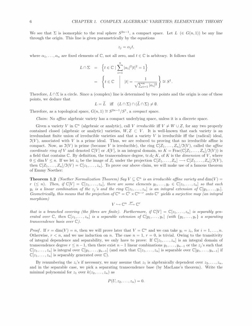
We see that Σ is isomorphic to the real sphere S2n−1, a compact space. Let L (∈ G(n, 1)) be any linethrough the origin. This line is given parametrically by the equations
zj = αjt,
where α1, . . . , αn are fixed elements of C, not all zero, and t ∈ C is arbitrary. It follows that
L ∩ Σ ={t ∈ C |
n∑i=1
|αi|2|t|2 = 1}
=
{t ∈ C
∣∣∣∣∣ |t| = 1√∑ni=1 |αi|2
}∼= S1.
Therefore, L∩Σ is a circle. Since a (complex) line is determined by two points and the origin is one of thesepoints, we deduce that
L = L iff (L ∩ Σ) ∩ (L ∩ Σ) �= ∅.Therefore, as a topological space, G(n, 1) ∼= S2n−1/S1, a compact space.
Claim: No affine algebraic variety has a compact underlying space, unless it is a discrete space.
Given a variety V in Cn (algebraic or analytic), call V irreducible iff V �= W ∪ Z, for any two properly
contained closed (algebraic or analytic) varieties, W,Z ⊂ V . It is well-known that each variety is anirredundant finite union of irreducible varieties and that a variety V is irreducible iff the (radical) ideal,I(V ), associated with V is a prime ideal. Thus, we are reduced to proving that no irreducible affine iscompact. Now, as I(V ) is prime (because V is irreducible), the ring C[Z1, . . . , Zn]/I(V ), called the affinecoordinate ring of V and denoted C[V ] or A[V ], is an integral domain, so K = Frac(C[Z1, . . . , Zn]/I(V )) isa field that contains C. By definition, the transcendence degree, tr.dC K, of K is the dimension of V , where0 ≤ dimV ≤ n. If we let zi be the image of Zi under the projection C[Z1, . . . , Zn] −→ C[Z1, . . . , Zn]/I(V ),then C[Z1, . . . , Zn]/I(V ) = C[z1, . . . , zn]. To prove our above claim, we will make use of a famous theoremof Emmy Noether:
Theorem 1.2 (Noether Normalization Theorem) Say V ⊆ Cn is an irreducible affine variety and dim(V ) =
r (≤ n). Then, if C[V ] = C[z1, . . . , zn], there are some elements y1, . . . , yr ∈ C[z1, . . . , zn] so that eachyi is a linear combination of the zj’s and the ring C[z1, . . . , zn] is an integral extension of C[y1, . . . , yr].Geometrically, this means that the projection of C
n = Cr×C
n−r onto Cr yields a surjective map (an integral
morphism)V ↪→ C
n pr−→ Cr
that is a branched covering (the fibres are finite). Furthermore, if C[V ] = C[z1, . . . , zn] is separably gen-erated over C, then C[z1, . . . , zn] is a separable extension of C[y1, . . . , yr] (with {y1, . . . , yr} a separatingtranscendence basis over C).
Proof . If r = dim(V ) = n, then we will prove later that V = Cn and we can take yi = zi, for i = 1, . . . , n.
Otherwise, r < n, and we use induction on n. The case n = 1, r = 0, is trivial. Owing to the transitivityof integral dependence and separability, we only have to prove: If C[z1, . . . , zn] is an integral domain oftranscendence degree r ≤ n− 1, then there exist n− 1 linear combinations y1, . . . , yn−1 or the zj ’s such thatC[z1, . . . , zn] is integral over C[y1, . . . , yn−1] (and such that C[z1, . . . , zn] is separable over C[y1, . . . , yn−1] ifC[z1, . . . , zn] is separably generated over C).
By renumbering the zi’s if necessary, we may assume that z1 is algebraically dependent over z2, . . . , zn,and in the separable case, we pick a separating transcendence base (by MacLane’s theorem). Write theminimal polynomial for z1 over k(z2, . . . , zn) as
P (U, z2, . . . , zn) = 0.

1.1. WHAT IS GEOMETRY & WHAT IS COMPLEX ALGEBRAIC GEOMETRY? 7
We can assume that the coefficients of P (U, z2, . . . , zn) are in C[z2, . . . , zn], so that the polynomialP (U, z2, . . . , zn) is the result of substituting U, z2, . . . , zn for X1,X2, . . . , Xn in some non-zero polynomialP (X1, . . . , Xn) with coefficients in C. Perform the linear change of variables
yj = zj − ajz1, for j = 2, . . . , n, (†)
and where a2, . . . , an ∈ C will be determined later. Since zj = yj + ajz1, it is sufficient to prove that z1is integral (and separable in the separable case) over C[y2, . . . , yn]. The minimal equation P (z1, z) = 0(abbreviating P (z1, z2, . . . , zn) by P (z1, z)) becomes
P (z1, y2 + a2z1, . . . , yn + anz1) = 0,
which can be written as
P (z1, y) = zq1f(1, a2, . . . , an) +Q(z1, y2, . . . , yn) = 0, (∗∗)
where f(X1,X2, . . . , Xn) is the highest degree form of P (X1, . . . , Xn) and q its degree, and Q contains termsof degree lower than q in z1. If we can find some aj ’s such that f(1, a2, . . . , an) �= 0, then we have anintegral dependence of z1 on y2, . . . , yn; thus, the zj ’s are integrally dependent on y2, . . . , yn, and we finishby induction. In the separable case, we need the minimal polynomial for z1 to have a simple root, i.e.,
dP
dz1(z1, y) �= 0.
We havedP
dz1(z1, y) =
∂P
∂z1(z1, z) + a2
∂P
∂z2(z1, z) + · · ·+ an
∂P
∂zn(z1, z).
But this is a linear form in the aj ’s which is not identically zero, since it takes for a2 = · · · = an = 0 thevalue
∂P
∂z1(z1, z) �= 0,
z1 being separable over C(z2, . . . , zn). Thus, the equation
∂P
∂x1(z1, z) + a2
∂P
∂z2(z1, z) + · · ·+ an
∂P
∂zn(z1, z) = 0
defines an affine hyperplane, i.e., the translate of a (linear) hyperplane. But then,
dP
dz1(z1, z) �= 0
on the complement of a hyperplane, that is, an infinite open subset of Cn−1, since C is infinite. On this
infinite set where dPdz1
(z1, z) �= 0, we can find a2, . . . , an so that f(1, a2, . . . , an) �= 0, which concludes theproof.
Now, we know that our G(n, 1) cannot be affine (i.e., of the form (†)) as it is compact(G(n, 1) ∼= S2n−1/S1). However, were G(n, 1) affine, Noether’s theorem would imply that C
r is compact, acontradiction. Therefore, G(n, 1) is not an affine variety.
However, observe that G(n, 1) is locally affine, i.e., it is an algebraic variety. Indeed a line, L, correspondsto a tuple (α1, . . . , αn) ∈ C
n with not all αj = 0. So, we can multiply by any λ ∈ C∗ and not change the
line. Look atUj = {(α1, . . . , αn) ∈ C
n | αj �= 0}.We have G(n, 1) =
⋃nn=1 Uj . On Uj , if we use λ = 1/αj as a multiplier, we get(
α1
αj, . . . ,
αj−1
αj, 1,
αj+1
αj, . . . ,
αnαj
),

8 CHAPTER 1. COMPLEX ALGEBRAIC VARIETIES; ELEMENTARY THEORY
so we see that Uj is canonically Cn−1. The patching on the overlaps is the previous glueing which gave P
n−1C
(with its functions). Therefore, we haveG(n, 1) = P
n−1C
.
1.2 Local Structure of Complex Varieties; Implicit Function The-orems and Tangent Spaces
We have the three ringsC[Z1, . . . , Zn] ⊆ C{Z1, . . . , Zn} ⊆ C[[Z1, . . . , Zn]],
where C{Z1, . . . , Zn} is the ring of convergent powers series, which means that for every power series inC{Z1, . . . , Zn} there is some open ball Bε containing the origin so that f � Bε converges, and C[[Z1, . . . , Zn]]is the ring of all power series, i.e., the ring of formal power series.
Remarks: (on (formal) power series).
Say A is a commutative ring (say, one of C{Z1, . . . , Zn} or C[[Z1, . . . , Zn]]) and look at A[[X1, . . . , Xn]] =B.
(1) f ∈ B is a unit (in B) iff f(0, . . . , 0) is a unit of A.
(2) B is a local ring iff A is a local ring, in which case the unique maximal ideal of B ismB = {f ∈ B | f(0, . . . , 0) ∈ mA}.
(3) B is noetherian iff A is noetherian (OK for us).
(4) If A is a domain then B is a domain.
(5) If B is a local ring, write B = lim←−n
B/mnB, the completion of B. We know that B has the m-adic
topology, where a basis of opens at 0 is given by the miB , with i ≥ 0. The topology in B is given by
the mnBB and the topology in B and B is Hausdorff iff
⋂∞n=0 mn
B = (0), which holds in the noetheriancase, by Krull’s theorem.
The fundamental results in this case are all essentially easy corollaries of the following lemma:
Lemma 1.3 Let O be a complete Hausdorff local domain with respect to the m-adic topology, and letf ∈ O[[X]]. Assume that
(a) f(0) ∈ m.
(b)(dfdX
)(0) is a unit of O.
Then, there exist unique elements α ∈ m and u(X) ∈ O[[X]], so that
(1) u(X) is a unit of O[[X]].
(2) f(X) = u(X)(X − α).
Proof . We get u(X) and α by successive approximations as follows. Refer to equation (2) by (†) in whatfollows. We compute the unknown coefficients of u(X) and the element α by successive approximations.Write u(X) =
∑∞j=0 ujX
j and f(X) =∑∞j=0 ajX
j ; reduce the coefficients modulo m in (†); then, sinceα ∈ m, (†) becomes
f(X) = Xu(X),
1.2. LOCAL STRUCTURE OF COMPLEX VARIETIES 9
which implies that∞∑j=0
ajXj =
∞∑j=0
ujXj+1.
Since a0 = 0, we have a0 ∈ m and uj = aj+1. Thus,
uj = aj+1 (mod m).
Note that
u0 = a1 =∂f
∂X(0) �= 0
in κ = O/m, which implies that if u(X) exists at all, then it is a unit. Write
uj = aj+1 + ξ(1)j ,
where ξ(1)j ∈ m, j ≥ 0. Remember that α ∈ m; so, upon reducing (†) modulo m2, we get
f(X) = u(X)(X − α).
This implies that
∞∑j=0
ajXj =
∞∑j=0
ujXj(X − α)
=∞∑j=0
ujXj+1 −
∞∑j=0
uj αXj
=∞∑j=0
(aj+1 + ξ
(1)j
)Xj+1 −
∞∑j=0
(aj+1 + ξ
(1)j
)αXj
=∞∑j=0
aj+1Xj+1 +
∞∑j=0
ξ(1)j Xj+1 −
∞∑j=0
aj+1 αXj .
Equating the constant coefficients, we geta0 = −a1 α.
Since a1 is a unit, α exists. Now, looking at the coefficient of Xj+1, we get
aj+1 = aj+1 + ξ(1)j − aj+2α,
which implies that
ξ(1)j = aj+2α,
and ξ(1)j exists.
We now proceed by induction. Assume that we know the coefficients u(t)j ∈ O of the t-th approximation
to u(X) and that u(X) using these coefficients (mod mt+1) works in (†), and further that the u(t)l ’s are
consistent for l ≤ t. Also, assume α(t) ∈ m, that α(t) (mod mt+1) works in (†), and that the α(l) areconsistent for l ≤ t. Look at u(t)
j + ξ(t+1)j , α(t) + η(t+1), where ξ(t+1)
j , η(t+1) ∈ mt+1. We want to determine

10 CHAPTER 1. COMPLEX ALGEBRAIC VARIETIES; ELEMENTARY THEORY
ξ(t+1)j and η(t+1), so that (†) will work for these modulo mt+2. For simplicity, write bar as a superscript to
denote reduction modulo mt+2. Then, reducing (†) modulo mt+2, we get∞∑j=0
ajXj =
∞∑j=0
ujXj(X − α)
=∞∑j=0
ujXj+1 −
∞∑j=0
uj αXj
=∞∑j=0
(u
(t)j + ξ
(t+1)j
)Xj+1 −
∞∑j=0
(u
(t)j + ξ
(t+1)j
)(α(t) + η(t+1)
)Xj
=∞∑j=0
u(t)j Xj+1 +
∞∑j=0
ξ(t+1)j Xj+1 −
∞∑j=0
u(t)j α(t)Xj −
∞∑j=0
u(t)j η(t+1)Xj .
Equating the constant coefficients, we get
a0 = −u(t)0 α(t) − u(t)
0 η(t+1).
But u(t)0 is a unit, and so, η(t+1) exists. Now, look at the coefficient of Xj+1, we have
aj+1 = u(t)j + ξ
(t+1)j − u(t)
j+1 α(t) − u(t)
j+1 η(t+1).
But u(t)j+1 α
(t) and u(t)j+1 η
(t+1) are now known and in mt+1 modulo mt+2, and thus,
ξ(t+1)j = aj+1 − u(t)
j + u(t)j+1 α
(t) + u(t)j+1 η
(t+1)
exists and the induction step goes through. As a consequence
u(X) ∈ lim←−t
(O/mt)[[X]]
andα ∈ lim←−
t
(m/mt)[[X]]
exist; and so, u(X) ∈ O[[X]] = O[[X]], and α ∈ m = m.
We still have to prove the uniqueness of u(X) and α. Assume that
f = u(X − α) = u(X − α).
Since u is a unit,u−1u(X − α) = X − α.
Thus, we may assume that u = 1. Since α ∈ m, we can plug α into the power series which defines u, andget convergence in the m-adic topology of O. We get
u(α)(α− α) = α− α,
so that α = α. Then,u(X − α) = X − α,
and since we assumed that O is a domain, so is O[[X]], and thus, u = 1.
Suppose that instead of dfdX (0) being a unit, we have f(0), . . . , d
r−1fdXr−1 (0) ∈ m, but drf
dXr (0) is a unit. We
can apply the fundamental lemma to f = dr−1fdXr−1 and then, we can apply (a rather obvious) induction and
get the general form of the fundamental lemma:

1.2. LOCAL STRUCTURE OF COMPLEX VARIETIES 11
Lemma 1.4 Let O be a complete Hausdorff local domain with respect to the m-adic topology, and letf ∈ O[[X]]. Assume that
(a) f(0), . . . , dr−1f
dXr−1 (0) ∈ m and
(b) drfdrX (0) is a unit of O (r ≥ 1).
Then, there exist unique elements α1, . . . , αr ∈ m and a unique power series u(X) ∈ O[[X]], so that
f(X) = u(X)(Xr + α1Xr−1 + · · ·+ αr−1X + αr)
and u(X) is a unit of O[[X]].
From the above, we get
Theorem 1.5 (Formal Weierstrass Preparation Theorem) Given f ∈ C[[Z1, . . . , Zn]], suppose
f(0, . . . , 0) =∂f
∂Z1(0) = · · · = ∂r−1f
∂Zr−11
(0) = 0, yet∂rf
∂Zr1(0) �= 0.
Then, there exist unique power series, u(Z1, . . . , Zn), gj(Z2, . . . , Zn), with 1 ≤ j ≤ r, so that
(1) u(Z1, . . . , Zn) is a unit
(2) gj(0, . . . , 0) = 0, where 1 ≤ j ≤ r and
(3) f(Z1, . . . , Zn) = u(Z1, . . . , Zn)(Zr1 + g1(Z2, . . . , Zn)Zr−11 + · · ·+ gr(Z2, . . . , Zn)).
Proof . Let O = C[[Z2, . . . , Zn]], then O[[Z1]] = C[[Z1, . . . , Zn]] and we have
df
dZ1=
∂f
∂Z1.
Thus, djf
dZj1(0) = 0 for j = 0, . . . , r − 1, so djf
dZj1(0) is a non-unit in O[[Z1]] for j = 0, . . . , r − 1, yet drf
dZr1(0) is a
unit. If we let αj of the fundamental lemma be gj(Z2, . . . , Zn), then each gj(Z2, . . . , Zn) vanishes at 0 (elseαj /∈ m) and the rest is obvious.
Theorem 1.6 (First form of the implicit function theorem) Given f ∈ C[[Z1, . . . , Zn]], if
f(0, . . . , 0) = 0 and∂f
∂Z1(0) �= 0,
then there exist unique power series u(Z1, . . . , Zn) and g(Z2, . . . , Zn) so that u(Z1, . . . , Zn) is a unit,g(0, . . . , 0) = 0, and f(Z1, . . . , Zn) factors as
f(Z1, . . . , Zn) = u(Z1, . . . , Zn)(Z1 − g(Z2, . . . , Zn)). (∗)
Moreover, every power series h(Z1, . . . , Zn) factors uniquely as
h(Z1, . . . , Zn) = f(Z1, . . . , Zn)q(Z1, . . . , Zn) + r(Z2, . . . , Zn).
Hence, there is a canonical isomorphism
C[[Z1, . . . , Zn]]/(f) ∼= C[[Z2, . . . , Zn]],
so that the following diagram commutes
C[[Z1, . . . , Zn] �� C[[Z1, . . . , Zn]]/(f)
C[[Z2, . . . , Zn]
��������������
����������������

12 CHAPTER 1. COMPLEX ALGEBRAIC VARIETIES; ELEMENTARY THEORY
Proof . Observe that equation (∗) (the Weierstrass preparation theorem) implies the second statement. For,assume (∗); then, u is a unit, so there is v such that vu = 1. Consequently,
vf = Z1 − g(Z2, . . . , Zn),
and the ideal (f) equals the ideal (vf), because v is a unit. So,
C[[Z1, . . . , Zn]]/(f) = C[[Z1, . . . , Zn]]/(vf),
and we get the residue ring by setting Z1 equal to g(Z2, . . . , Zn). It follows that the canonical isomorphism
C[[Z1, . . . , Zn]]/(f) ∼= C[[Z2, . . . , Zn]]
is given as follows: In h(Z1, . . . , Zn), replace every occurrence of Z1 by g(Z2, . . . , Zn); we obtain
h(Z2, . . . , Zn) = h(g(Z2, . . . , Zn), Z2, . . . , Zn),
and the diagram obviously commutes. Write r(Z2, . . . , Zn) instead of h(Z2, . . . , Zn). Then,
h(Z1, . . . , Zn)− r(Z2, . . . , Zn) = fq
for some q(Z1, . . . , Zn). We still have to show uniqueness. Assume that
h(Z1, . . . , Zn) = fq + r = f q + r.
Since g(0, . . . , 0) = 0, we have g ∈ m; thus, we can plug in Z1 = g(Z2, . . . , Zn) and get m-adic convergence.By (∗), f goes to 0, and the commutative diagram shows r (mod f) = r and r (mod f) = r. Hence, we get
r = r,
so thatfq − f q = 0.
Now, C[[Z1, . . . , Zn]] is a domain, so q = q.
We can now apply induction to get the second version of the formal implicit function theorem, or FIFT .
Theorem 1.7 (Second form of the formal implicit function theorem)Given f1, . . . , fr ∈ C[[Z1, . . . , Zn]], if fj(0, . . . , 0) = 0 for j = 1, . . . , r and
rk(∂fi∂Zj
(0))
= r
(so that n ≥ r), then we can reorder the variables so that
rk(∂fi∂Zj
(0))
= r, where 1 ≤ i, j ≤ r,
and there is a canonical isomorphism
C[[Z1, . . . , Zn]]/(f1, . . . , fr) ∼= C[[Zr+1, . . . , Zn]],
which makes the following diagram commute
C[[Z1, . . . , Zn]] �� C[[Z1, . . . , Zn]]/(f1, . . . , fr)
C[[Zr+1, . . . , Zn]]
���������������
������������������

1.2. LOCAL STRUCTURE OF COMPLEX VARIETIES 13
Proof . The proof of this statement is quite simple (using induction) from the previous theorem (DX).
What becomes of these results for the convergent case? They hold because we can make estimatesshowing all processes converge for C. However, these arguments are tricky and messy (they can be foundin Zariski and Samuel, Volume II [15]). In our case, we can use complex analysis. For any ξ ∈ C
n and anyε > 0, we define the polydisc of radius ε about ξ, PD(ξ, ε), by
PD(ξ, ε) = {(z1, . . . , zn) ∈ Cn | |zi − ξi| < ε, for every i, 1 ≤ i ≤ n}.
Say f(Z1, . . . , Zn) is holomorphic near the origin and suppose f(0, . . . , 0) = ∂f∂Z1
(0) = · · · = ∂r−1f
∂Zr−11
(0) = 0
and ∂rf∂Zr
1(0) �= 0, Consider f as a function of Z1, with ‖(Z2, . . . , Zn)‖ < ε, for some ε > 0. Then, f will have
r zeros, each as a function of Z2, . . . , Zn in the ε-disc. Now, we know (by one-dimensional Cauchy theory)that
ηq1 + · · ·+ ηqr =1
2πi
∫|ξ|=R
ξq ∂f∂Z1
(ξ, Z2, . . . , Zn)f(ξ, Z2, . . . , Zn)
dξ,
where η1, . . . , ηr are the roots (as functions of Z2, . . . , Zn) and q is any integer ≥ 0. Therefore, the powersums of the roots are holomorphic functions of Z2, . . . , Zn. By Newton’s identities, the elementary symmetricfunctions σj(η1, . . . , ηr), for j = 1, . . . , r, are polynomials in the power sums, call these elementary symmetricfunctions g1(Z2, . . . , Zn), . . . , gr(Z2, . . . , Zn). Then, the polynomial
w(Z1, . . . , Zn) = Zr1 − g1(Z2, . . . , Zn)Zr−11 + · · ·+ (−1)rgr(Z2, . . . , Zn)
vanishes exactly where f vanishes. Look at f(Z1, . . . , Zn)/w(Z1, . . . , Zn) off the zeros. Then, the latter asa function of Z1 has only removable singularities. Thus, by Riemann’s theorem, this function extends to aholomorphic function in Z1 on the whole disc. As f/w is holomorphic in Z1, by the Cauchy integral formula,we get
u(Z1, . . . , Zn) =f(Z1, . . . , Zn)w(Z1, . . . , Zn)
=1
2πi
∫|ξ|=R
u(ξ, Z2, . . . , Zn)ξ − Z1
dξ.
Yet, the right hand side is holomorphic in Z2, . . . , Zn, which means that u(Z1, . . . , Zn) is holomorphic ina polydisc and as we let the Zj go to 0, the function u(Z1, . . . , Zn) does not vanish as the zeros cancel.Consequently, we have
f(Z1, . . . , Zn) = u(Z1, . . . , Zn)(Zr1 + g1(Z2, . . . , Zn)Zr−11 + · · ·+ gr(Z2, . . . , Zn)).
Theorem 1.8 (Weierstrass Preparation Theorem (Convergent Case)) Given f ∈ C{Z1, . . . , Zn}, suppose
f(0, . . . , 0) =∂f
∂Z1(0) = · · · = ∂r−1f
∂Zr−11
(0) = 0, yet∂rf
∂Zr1(0) �= 0.
Then, there exist unique power series, u(Z1, . . . , Zn), gj(Z2, . . . , Zn) in C{Z1, . . . , Zn}, with 1 ≤ j ≤ r, andsome ε > 0, so that
(1) u(Z1, . . . , Zn) is a unit
(2) gj(0, . . . , 0) = 0, where 1 ≤ j ≤ r and
(3) f(Z1, . . . , Zn) = u(Z1, . . . , Zn)(Zr1 + g1(Z2, . . . , Zn)Zr−11 + · · ·+ gr(Z2, . . . , Zn)), in some polydisc
PD(0, ε).
Proof . Existence has already been proved. If more than one solution exists, read in C[[Z1, . . . , Zn]] andapply uniqueness there.
As a consequence, we obtain the implicit function theorem and the inverse function theorem in theconvergent case.

14 CHAPTER 1. COMPLEX ALGEBRAIC VARIETIES; ELEMENTARY THEORY
Theorem 1.9 (Implicit Function Theorem (First Form–Convergent Case)) Let f ∈ C{Z1, . . . , Zn} andsuppose that f(0, . . . , 0) = 0, but
∂f
∂Z1(0, . . . , 0) �= 0.
Then, there exists a unique power series g(Z2, . . . , Zn) ∈ C{Z2 . . . , Zn} and there is some ε > 0, so that inthe polydisc PD(0, ε), we have f(Z1, . . . , Zn) = 0 if and only if Z1 = g(Z2, . . . , Zn). Furthermore, the maph �→ h = h(g(Z2, . . . , Zn), Z2, . . . , Zn) gives rise to the commutative diagram
C{Z1, . . . , Zn} �� C{Z1, . . . , Zn}/(f)
C{Z2, . . . , Zn}
���������������
����������������
Proof . (DX).
An easy induction yields
Theorem 1.10 (Convergent implicit function theorem) Let f1, . . . , fr ∈ C{Z1, . . . , Zn}. If fj(0, . . . , 0) = 0for j = 1, . . . , r and
rk(∂fi∂Zj
(0))
= r
(so that n ≥ r), then there is a permutation of the variables so that
rk(∂fi∂Zj
(0))
= r, where 1 ≤ i, j ≤ r
and there exist r unique power series gj(Zr+1, . . . , Zn) ∈ C{Zr+1 . . . , Zn} (1 ≤ j ≤ r) and an ε > 0, so thatin the polydisc PD(0, ε), we have
f1(ξ) = · · · = fr(ξ) = 0 iff ξj = gj(ξr+1, . . . , ξn), for j = 1, . . . , r.
MoreoverC{Z1, . . . , Zn}/(f1, . . . , fr) ∼= C{Zr+1, . . . , Zn}
and the following diagram commutes:
C{Z1, . . . , Zn} �� C{Z1, . . . , Zn}/(f1, . . . , fr)
C{Zr+1, . . . , Zn}
���������������
������������������
When r = n, we have another form of the convergent implicit function theorem also called the inversefunction theorem.
Theorem 1.11 (Inverse function theorem) Let f1, . . . , fn ∈ C{Z1, . . . , Zn} and suppose that fj(0, . . . , 0) = 0for j = 1, . . . , n, but
rk(∂fi∂Zj
(0, . . . , 0))
= n.
Then, there exist n unique power series gj(W1, . . . ,Wn) ∈ C{W1 . . . ,Wn} (1 ≤ j ≤ n) and there are someopen neighborhoods of (0, . . . , 0) (in the Z’s and in the W ’s), call them U and V , so that the holomorphicmaps
(Z1, . . . , Zn) �→ (W1 = f1(Z1, . . . , Zn), . . . ,Wn = fn(Z1, . . . , Zn)) : U → V
(W1, . . . ,Wn) �→ (Z1 = g1(W1, . . . ,Wn), . . . , Zn = gn(W1, . . . ,Wn)) : V → U
are inverse isomorphisms.

1.2. LOCAL STRUCTURE OF COMPLEX VARIETIES 15
In order to use these theorems, we need a linear analysis via some kind of “tangent space.” Recall thata variety, V , is a union of affine opens
V =⋃α
Vα.
Take ξ ∈ V , then there is some α (perhaps many) so that ξ ∈ Vα. Therefore, assume at first that V is affineand say V ⊆ C
n and is cut out by the radical ideal A = I(V ) = (f1, . . . , fp). Pick any f ∈ A and write theTaylor expansion for f at ξ ∈ C
n:
f(Z1, . . . , Zn) = f(ξ) +n∑j=1
(∂f
∂Zj
)ξ
(Zj − ξj) +O(quadratic).
Since ξ ∈ V , we have f(ξ) = 0. This suggests looking at the linear form
lf,ξ(λ1, . . . , λn) =n∑j=1
(∂f
∂Zj
)ξ
λj , where λj = Zj − ξj .
Examine the linear subspace
⋂f∈A
Ker lf,ξ =
(λ1, . . . , λn) ∈ Cn
∣∣∣∣∣∣ (∀f ∈ A)
n∑j=1
(∂f
∂Zj
)ξ
λj = 0
. (∗)
Note that as f =∑ti=1 hifi, where hi ∈ C[Z1, . . . , Zn], we get
∂f
∂Zj=
t∑i=1
(hi∂fi∂Zj
+ fi∂hi∂Zj
),
and, since fi(ξ) = 0, (∂f
∂Zj
)ξ
=t∑i=1
hi(ξ)(∂fi∂Zj
)ξ
.
The equation in (∗) becomesn∑j=1
t∑i=1
(hi(ξ)
(∂fi∂Zj
)ξ
)(Zj − ξj) = 0,
which yieldst∑i=1
hi(ξ)
n∑j=1
(∂fi∂Zj
)ξ
(Zj − ξj)
= 0.
Hence, the vector space defined by (∗) is also defined by
n∑j=1
(∂fi∂Zj
)ξ
(Zj − ξj) = 0, for i = 1, . . . , t. (∗∗)
Definition 1.1 The linear space at ξ ∈ V defined by (∗∗) is called the Zariski tangent space at ξ of V . Itis denoted by TV,ξ.
Note that Definition 1.1 is an extrinsic definition. It depends on the embedding of V in Cn, but assume
for the moment that it is independent of the embedding. We have the following proposition:

16 CHAPTER 1. COMPLEX ALGEBRAIC VARIETIES; ELEMENTARY THEORY
Proposition 1.12 Let V be an irreducible complex variety. The function
ξ �→ dimCTV,ξ
is upper-semicontinuous on V , i.e.,
Sl = {ξ ∈ V | dimCTV,ξ ≥ l}
is Z-closed in V , and furthermore, Sl+1 ⊆ Sl and it is Z-closed in Sl.
Proof . Since we are assuming that TV,ξ is independent of the particular affine patch where ξ finds itself, wemay assume that V is affine. So, TV,ξ is the vector space given by the set of (λ1, . . . , λn) ∈ C
n such that
n∑j=1
(∂fi∂Zj
)ξ
λj = 0, for i = 1, . . . ,m,
where f1, . . . , fm generate the ideal A = I(V ). Hence, TV,ξ is the kernel of the linear map from Cn to C
m
given by the m× n matrix ((∂fi∂Zj
)ξ
).
It follows that
dimCTV,ξ = n− rk
((∂fi∂Zj
)ξ
).
Consequently, dimCTV,ξ ≥ l iff
rk
((∂fi∂Zj
)ξ
)≤ n− l;
and this holds iff the (n− l + 1)× (n− l + 1) minors are all singular at ξ. But the latter is true when andonly when the corresponding determinants vanish at ξ. These give additional equations on V at ξ in orderthat ξ ∈ Sl and this implies that Sl is Z-closed in V . That Sl+1 ⊆ Sl is obvious and since Sl+1 is given bymore equations, Sl+1 is Z-closed in Sl.
We now go back to the question: Is the definition of the tangent space intrinsic?
It is possible to give an intrinsic definition. For this, we review the notion of C-derivation. Let M be aC-module and recall that A[V ] = C[Z1, . . . , Zn]/I(V ), the affine coordinate ring of V .
Definition 1.2 A C-derivation of A[V ] with values in M centered at ξ consists of the following data:
(1) A C-linear map D : A[V ]→M . (values in M)
(2) D(fg) = f(ξ)Dg + g(ξ)Df (Leibnitz rule) (centered at ξ)
(3) D(λ) = 0 for all λ ∈ C. (C-derivation)
The set of such derivations is denoted by DerC(A[V ],M ; ξ).
The compositionC[Z1, . . . , Zn] −→ A[V ] D−→M
is again a C-derivation (on the polynomial ring) centered at ξ with values in M . Note that a C-derivationon the polynomial ring (call it D again) factors as above iff D � I(V ) = 0. This shows that
DerC(A[V ],M ; ξ) = {D ∈ DerC(C[Z1, . . . , Zn],M ; ξ) | D � I(V ) = 0}.
1.2. LOCAL STRUCTURE OF COMPLEX VARIETIES 17
However, a C-derivation D ∈ DerC(C[Z1, . . . , Zn],M ; ξ) is determined by its values D(Zj) = λj at thevariables Zj . Clearly (DX),
D(f(Z1, . . . , Zn)) =n∑j=1
(∂f
∂Zj
)ξ
D(Zj).
But, observe that for any (λ1, . . . , λn), the restriction of D to I(V ) vanishes iff
n∑j=1
(∂f
∂Zj
)ξ
λj = 0, for every f ∈ I(V ),
that is, iffn∑j=1
(∂fi∂Zj
)ξ
λj = 0, for every i = 1, . . . ,m,
where f1, . . . , fm generate the ideal I(V ). Letting ηj = λj + ξj ∈ M (with ξi ∈ M), we have a bijectionbetweenDerC(A[V ],M ; ξ) and (η1, . . . , ηn) ∈Mn
∣∣∣∣∣∣n∑j=1
(∂fi∂Zj
)ξ
λj = 0, 1 ≤ i ≤ m
.
It is given by the mapD �→ (η1, . . . , ηn),
with ηj = D(Zj) + ξj . This gives the isomorphism
TV,ξ ∼= DerC(A[V ],C; ξ).
We conclude that TV,ξ is independent of the embedding of V into Cn, up to isomorphism.
Take V to be irreducible to avoid complications. Then, A[V ] is an integral domain (as I(V ) is a primeideal) and so, OV,ξ = A[V ]I(ξ), the localization of A[V ] at the prime ideal I(ξ) consisting of all g ∈ A[V ]where g(ξ) = 0. This is because elements of the local ring OV,ξ are equivalence classes of ratios f/g, wheref, g ∈ A[V ] with g(ξ) �= 0 (where g is zero is Z-closed and so, the latter is Z-open), with f/g ∼ f/g iff f/g
and f/g agree on a small neighborhood of ξ. On the Z-open where gg �= 0, we get fg−gf = 0 iff f/g ∼ f/g.By analytic continuation, we get fg − gf = 0 in A[V ]. Therefore, OV,ξ = A[V ]I(ξ).
It follows that
OV,ξ ={[
f
g
] ∣∣∣∣ f, g ∈ A[V ], g /∈ I(ξ)}
={[
f
g
] ∣∣∣∣ f, g ∈ A[V ], g(ξ) �= 0}.
Any C-derivation D ∈ DerC(A[V ],M ; ξ) is uniquely extendable to OV,ξ via
D
(f
g
)=g(ξ)Df − f(ξ)Dg
g(ξ)2.
Therefore,DerC(A[V ],C; ξ) = DerC(OV,ξ,C; ξ).
There are some difficulties when V is reducible. As an example in C3, consider the union of a plane and
an algebraic curve piercing that plane, with ξ any point of intersection.
18 CHAPTER 1. COMPLEX ALGEBRAIC VARIETIES; ELEMENTARY THEORY
Remark: Since the Sl manifestly form a nonincreasing chain as l increases, there is a largest l for whichSl = V . The set Sl+1 is closed in V , and its complement {ξ | dimCTV,ξ = l} is Z-open. This gives us thetangent space stratification (a disjoint union) by locally closed sets (a locally closed set is the intersection ofan open set with a closed set)
V = U0 ∪· U1 ∪· · · · ∪· Ut,where U0 = {ξ | dimC TV,ξ = l} is open, and Ui = {ξ | dimC TV,ξ = l + i}. We have U1 open inV − U0 = Sl+1, etc.
Now, we have the first main result.
Theorem 1.13 Say V is a complex variety and suppose dimCV = supα dimCVα <∞, where Vα is an affineopen in V ), e.g., V is quasi-compact (which means that V is a finite union of open affines). Then, there isa nonempty open (in fact, Z-open), U , in V so that for all ξ ∈ U ,
dimC TV,ξ = dimC V.
Moreover, for all ξ ∈ V , if V is irreducible, then dimC TV,ξ ≥ dimC V .
Proof . We have V =⋃α Vα, where each Vα is affine open and dimC V = supα dimC Vα ≤ ∞ so that
dimC V = dimC Vα, for some α and if the first statement of the theorem is true for Vα, then there is someopen, U ⊆ Vα, and as Vα is open itself, U is an open in V with the desired property. So, we may assumethat V is affine. Let
V = V1 ∪ · · · ∪ Vtbe an irredundant decomposition into irreducible components. At least one of the Vj ’s has dimension dim(V ).Say it is j = 1. Look at V1 ∩ Vj , j = 2, . . . , t. Each V1 ∩ Vj is a closed set, and so
W = V −t⋃
j=2
V1 ∩ Vj
is Z-open. Also, W ∩V1 is Z-open in V1 because it is the complement of all the closed sets V1∩Vj with j ≥ 2.Take any open subset, U , of V −
⋃tj=2 Vj for which U is a good open in V1, that is, where dimCTV,ξ = dimCV1
whenever ξ ∈ U . Then, U ∩W also has the right property. Hence, we may assume that V is affine andirreducible.
Write A[V ] for the coordinate ring C[Z1, . . . , Zn]/I(V ), where I(V ) is a prime ideal. Then, A[V ] is adomain and write K = Frac(A[V ]). I claim that
dimK DerC(K,K) = dimC V. (∗)
We know dim V = tr.dC K = tr.dC A[V ]. Pick a transcendence basis ζ1, . . . , ζr for A[V ], then A[V ] isalgebraic over C[ζ1, . . . , ζr]; therefore, A[V ] is separable over C[ζ1, . . . , ζr] (C has characteristic zero). Wehave the isomorphism
DerC(C[ζ1, . . . , ζr],K) −→ Kr,
and if α ∈ A[V ], then α satisfies an irreducible polynomial
ξ0αm + ξ1α
m−1 + · · ·+ ξm = 0,
where ξj ∈ C[ζ1, . . . , ζr] and α is a simple root. Let f(T ) =∑mi=0 ξiT
m−i, where T is some indeterminate.We have f(α) = 0 and f ′(α) �= 0. For any D ∈ DerC(C[ζ1, . . . , ζr],K), we have
0 = D(f(α)) = f ′(α)D(α) +m∑i=0
αm−iDξi,
1.2. LOCAL STRUCTURE OF COMPLEX VARIETIES 19
and as f ′(α) �= 0, we see that D(α) exists and is uniquely determined. Therefore,
DerC(C[ζ1, . . . , ζr],K) ∼= DerC(A[V ],K)
which proves (∗).Now, we have I(V ) = (f1, . . . , fp) and as we observed earlier
DerC(A[V ],K) ∼=
(λ1, . . . , λn) ∈ Kn
∣∣∣∣∣∣n∑j=1
(∂fi∂Zj
)λj = 0, 1 ≤ i ≤ p
.
Therefore,
dimC V = dimK Der(A[V ],K) = n− rk((
∂fi∂xj
)).
Let
s = rk((
∂fi∂xj
))where the above matrix has entries in K. By linear algebra, there are matrices A,B (with entries in K) sothat
A
(∂fi∂xj
)B =
(Ir 00 0
).
Let α(X1, . . . , Xn) and β(X1, . . . , Xn) be the common denominators of entries in A and B, respectively. So,A = (1/α)A and B = (1/β)B, and the entries in A and B are in A[V ]. Let U be the open set where thepolynomial αβ det(A) det(B) is nonzero. Then, as
1αβ
A
(∂fi∂xj
)B =
(Is 00 0
)in K,
for any ξ ∈ U , we have1
α(ξ)β(ξ)A(ξ)
((∂fi∂xj
)ξ
)B(ξ) =
(Ir 00 0
),
and ((∂fi∂xj
)ξ
)has rank s, a constant.
Now, if V is irreducible, we must have a big open subset U0 of V where dimTV,ξ is equal to the minimumit takes on V . Also, we have an open, U0, where dim TV,ξ = dim(V ). Since these opens are dense, we find
U0 ∩ U0 �= ∅.
Therefore, we must haveU0 = U0,
and the minimum value taken by the dimension of the Zariski tangent space is just dim(V ). In summary,the set
U0 = {ξ ∈ V | dim TV,ξ = dim(V )} = minξ∈V
dim TV,ξ
is a Z-open dense subset of V .
Remark: Say Vi and Vj are irreducible in some irredundant decomposition of V . If ξ ∈ Vi ∩ Vj (i �= j),check (DX) that dim TV,ξ ≥ dim TVi,ξ + dim TVj ,ξ.

20 CHAPTER 1. COMPLEX ALGEBRAIC VARIETIES; ELEMENTARY THEORY
V
Figure 1.2: Example of A Surface with Singularites
Definition 1.3 If V is an irreducible variety, a point ξ ∈ V is nonsingular if
dimC TV,ξ = dimC(V ).
Otherwise, we say that ξ is singular . If V is quasi-compact but not irreducible and ξ ∈ Vi ∩ Vj for twodistinct irreducible (irredundant) components of V , we also say that ξ is singular . The singular locus of Vis denoted by Sing(V ).
Remark: In the interest of brevity, from now on, we will assume that a complex variety is a quasi-compact(in the Z-topology) complex algebraic variety. A generalized complex variety is a complex variety that isHausdorff but not necessarily quasi-compact.
From previous observations, the singular locus, Sing(V ), of V is a Z-closed set, so it is a complex variety.This leads to the Zariski stratification. Let U0 be the set of nonsingular points in V , write V1 = Sing(V ) =V − U0, and let U1 be the set of nonsingular points in V1. We can set V2 = V1 − U1, and so on. Then, weobtain the Zariski-stratification of V into disjoint locally closed strata
V = U0 ∪· U1 ∪· · · · ∪· Ut,
where each Ui is a nonsingular variety and U0 is the open subset of nonsingular points in V .
Example 1.1 In this example (see Figure 1.2), Sing(V ) consists of a line with a bad point on it (the origin).V1 is that line, and V2 = Sing(V1) is the bad point.
1.2. LOCAL STRUCTURE OF COMPLEX VARIETIES 21
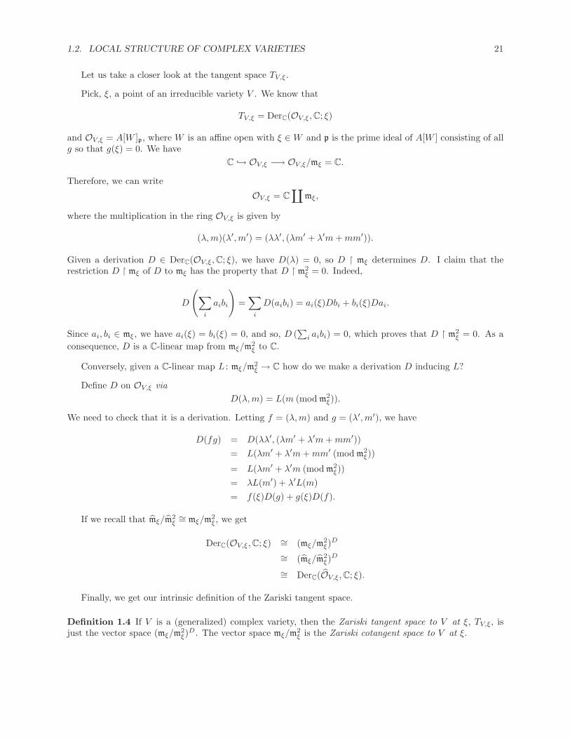
Let us take a closer look at the tangent space TV,ξ.
Pick, ξ, a point of an irreducible variety V . We know that
TV,ξ = DerC(OV,ξ,C; ξ)
and OV,ξ = A[W ]p, where W is an affine open with ξ ∈W and p is the prime ideal of A[W ] consisting of allg so that g(ξ) = 0. We have
C ↪→ OV,ξ −→ OV,ξ/mξ = C.
Therefore, we can write
OV,ξ = C
∐mξ,
where the multiplication in the ring OV,ξ is given by
(λ,m)(λ′,m′) = (λλ′, (λm′ + λ′m+mm′)).
Given a derivation D ∈ DerC(OV,ξ,C; ξ), we have D(λ) = 0, so D � mξ determines D. I claim that therestriction D � mξ of D to mξ has the property that D � m2
ξ = 0. Indeed,
D
(∑i
aibi
)=∑i
D(aibi) = ai(ξ)Dbi + bi(ξ)Dai.
Since ai, bi ∈ mξ, we have ai(ξ) = bi(ξ) = 0, and so, D (∑i aibi) = 0, which proves that D � m2
ξ = 0. As aconsequence, D is a C-linear map from mξ/m
2ξ to C.
Conversely, given a C-linear map L : mξ/m2ξ → C how do we make a derivation D inducing L?
Define D on OV,ξ viaD(λ,m) = L(m (mod m2
ξ)).
We need to check that it is a derivation. Letting f = (λ,m) and g = (λ′,m′), we have
D(fg) = D(λλ′, (λm′ + λ′m+mm′))= L(λm′ + λ′m+mm′ (mod m2
ξ))
= L(λm′ + λ′m (mod m2ξ))
= λL(m′) + λ′L(m)= f(ξ)D(g) + g(ξ)D(f).
If we recall that mξ/m2ξ∼= mξ/m
2ξ , we get
DerC(OV,ξ,C; ξ) ∼= (mξ/m2ξ)D
∼= (mξ/m2ξ)D
∼= DerC(OV,ξ,C; ξ).
Finally, we get our intrinsic definition of the Zariski tangent space.
Definition 1.4 If V is a (generalized) complex variety, then the Zariski tangent space to V at ξ, TV,ξ, isjust the vector space (mξ/m
2ξ)D. The vector space mξ/m
2ξ is the Zariski cotangent space to V at ξ.

22 CHAPTER 1. COMPLEX ALGEBRAIC VARIETIES; ELEMENTARY THEORY
1.3 Local Structure of Complex Varieties, II; Dimension and Useof the Implicit Function Theorem
Let V be an irreducible variety. For any ξ ∈ V , we have mξ, the maximal ideal of the local ring OV,ξ.Examine maximal chains of prime ideals of OV,ξ
mξ > p1 > · · · > pd = (0). (†)
Such chains exist and end with (0) since OV,ξ is a noetherian local domain. The length, d, of this chain isthe height of mξ. The Krull dimension of OV,ξ is the height of mξ (denoted dim OV,ξ). Since V is locallyaffine, every ξ ∈ V belongs to some affine open, so we may assume that V is affine, V ⊆ C
n and V is givenby a prime ideal I(V ). Thus, A[V ] = C[Z1, . . . , Zn]/I(V ) and OV,ξ = A[V ]P, where
P = {g ∈ A[V ] | g(ξ) = 0}.
Our chain (†) corresponds to a maximal chain of prime ideals
P > P1 > · · · > Pd = (0)
of A[V ] and the latter chain corresponds to a chain of irreducible subvarieties
{ξ} < V1 < · · · < Vd = V.
Therefore, the length d of our chains is on one hand the Krull dimension of OV,ξ and on the other hand itis the combinatorial dimension of V at ξ. Therefore,
ht mξ = dimOX,ξ = combinatorial dim. of V at ξ.
Nomenclature. Say V and W are affine and we have a morphism ϕ : V → W . This gives a map of
C-algebras, A[W ]Γ(ϕ)−→ A[V ]. Now, we say that
(1) ϕ is an integral morphism if Γ(ϕ) makes A[V ] a ring integral over A[W ].
(2) ϕ is a finite morphism if A[V ] a finitely generated A[W ]-module.
(3) If V and W are not necessarily affine and ϕ : V →W is a morphism, then ϕ is an affine morphism iffthere is an open cover of W by affines, Wα, so that ϕ−1(Wα) is again affine as a variety. Then, we cancarry over (1) and (2) to the general case via: A morphism ϕ is integral (resp. finite) iff
(a) ϕ is affine
(b) For every α, the morphism ϕ � ϕ−1(Wα) −→Wα is integral (resp. finite).
An irreducible variety, V , is a normal variety iff it has an open covering, V =⋃α Vα, so that A[Vα] is
integrally closed in its fraction field.
Proposition 1.14 Let V,W be irreducible complex varieties, with W normal. If dim(W ) = d and ϕ : V →W is a finite surjective morphism, then dim(V ) = d and ϕ establishes a surjective map from the collectionof closed Z-irreducible subvarieties of V to those of W , so that
(1) maximal irreducible subvarieties of V map to maximal irreducible subvarieties of W
(2) inclusion relations are preserved
(3) dimensions are preserved

1.3. LOCAL STRUCTURE OF COMPLEX VARIETIES, II 23
(4) no irreducible subvariety of V , except V itself, maps onto W .
Proof . Let Wα be an affine open in W , then so is Vα = ϕ−1(Wα) in V , because ϕ is affine, since it is a finitemorphism. If Z is an irreducible closed variety in V , then Zα = Z ∩Vα is irreducible in Vα since Zα is densein Z. Thus, we may assume that V and W are affine. Let A = A[W ] and B = A[V ]. Since ϕ is finite andsurjective, we see that Γ(ϕ) is an injection, so B is a finite A-module. Both A,B are integral domains, bothare Noetherian, A is integrally closed, and no nonzero element of A is a zero divisor in B. These are theconditions for applying the Cohen-Seidenberg theorems I, II, and III. As A[V ] is integral, therefore algebraicover A[W ], we have
d = dimW = tr.dC A[W ] = tr.dC A[V ] = dim V,
which shows that dimW = dim V .
By Cohen-Seidenberg I (Zariski and Samuel [14], Theorem 3, Chapter V, Section 2, or Atiyah andMacdonald [1], Chapter 5), there is a surjective correspondence
P �→ P ∩A
between prime ideals of B and prime ideals of A, and thus, there is a surjective correspondence betweenirreducible subvarieties of V and their images in W .
Consider a maximal irreducible variety Z in V . Then, its corresponding ideal is a minimal prime idealP. Let p = P∩A, the ideal corresponding to ϕ(Z). If ϕ(Z) is not a maximal irreducible variety in W , thenp is not a minimal prime, and thus, there is some prime ideal q of A such that
q ⊂ p,
where the inclusion is strict. By Cohen-Seidenberg III (Zariski and Samuel [14], Theorem 6, Chapter V,Section 3, or Atiyah and Macdonald [1], Chapter 5), there is some prime ideal Q in B such that
Q ⊂ P
and q = Q ∩ A, contradicting the fact that P is minimal. Thus, ϕ takes maximal irreducible varieties tomaximal irreducible varieties.
Finally, by Cohen-Seidenberg II (Zariski and Samuel [14], Corollary to Theorem 3, Chapter V, Section2, or Atiyah and Macdonald [1], Chapter 5), inclusions are preserved, and since ϕ is finite, dimension ispreserved. The rest is clear.
We can finally prove the fundamental fact on dimension.
Proposition 1.15 Let V and W be irreducible complex varieties with W a maximal subvariety of V . Then,
dim(W ) = dim(V )− 1.
Proof . We may assume that V and W are affine (using open covers, as usual). By Noether’s normalizationtheorem (Theorem 1.2), there is a finite surjective morphism ϕ : V → C
r, where r = dimC(V ). However, Cr
is normal, and by Proposition 1.14, we may assume that V = Cr. Let W be a maximal irreducible variety
in Cr. It corresponds to a minimal prime ideal P of A[T1, . . . , Tr], which is a UFD. As a consequence, since
P is a minimal prime, it is equal to some principal ideal, i.e., P = (g), where g is not a unit. Without lossof generality, we may assume that g involves Tr.
Now, the images t1, . . . , tr−1 of T1, . . . , Tr−1 in A[T1, . . . , Tr]/P are algebraically independent over C.Otherwise, there would be some polynomial f ∈ A[T1, . . . , Tr−1] such that
f(t1, . . . , tr−1) = 0.

24 CHAPTER 1. COMPLEX ALGEBRAIC VARIETIES; ELEMENTARY THEORY
But then, f(T1, . . . , Tr−1) ∈ P = (g). Thus,
f(T1, . . . , Tr−1) = α(T1, . . . , Tr)g(T1, . . . , Tr),
contradicting the algebraic independence of T1, . . . , Tr. Therefore, dimC(W ) ≥ r− 1, but since we also knowthat dimC(W ) ≤ r − 1, we get dimC(W ) = r − 1.
Corollary 1.16 The combinatorial dimension of V over {ξ} is just dimC V ; consequently, it is independentof ξ ∈ V (where V is affine irreducible).
Corollary 1.17 If V is affine and irreducible, then dimC mξ/m2ξ ≥ dimC V = comb. dim. V = dimC OV,ξ
(= Krull dimension) and we have equality iff ξ is a nonsingular point. Therefore, OV,ξ is a regular local ring(i.e., dimC mξ/m
2ξ = dimC OV,ξ) iff ξ is a nonsingular point.
We now use these facts and the implicit function theorem for local analysis near a nonsingular point.
Definition 1.5 Say V ⊆ Cn is an affine variety and write d = dim V . Then, V is called a complete
intersection iff I(V ) has n−d generators. If V is not necessarily affine and ξ ∈ V , then V is a local completeintersection at ξ iff there is some affine open, V (ξ), of V such that
(a) ξ ∈ V (ξ) ⊆ V
(b) V (ξ) ⊆ Cn, for some n, as a subvariety
(c) V (ξ) is a complete intersection in Cn.
Theorem 1.18 (Local Complete Intersection Theorem) Let V be an irreducible complex variety, ξ ∈ V bea nonsingular point and write dim(V ) = d. Then, V is a local complete intersection at ξ. That is, there issome affine open, U ⊆ V , with ξ ∈ U , such that U can be embedded into C
n as a Z-closed subset (we mayassume that n is minimal) and U is cut out by r = n−d polynomials. This means that there exists a possiblysmaller Z-open W ⊆ U ⊆ V with ξ ∈W and some polynomials f1, . . . , fr, so that
η ∈W if and only if f1(η) = · · · = fr(η) = 0.
The local complete intersection theorem will be obtained from the following affine form of the theorem.
Theorem 1.19 (Affine local complete intersection theorem) Let V ⊆ Cn be an affine irreducible complex
variety of dimension dim(V ) = d, and assume that V = V (p). If ξ ∈ V is nonsingular point, then there existf1, . . . , fr ∈ p, with r = n− d, so that
p =
{g ∈ C[Z1, . . . , Zn]
∣∣∣∣∣ g =r∑i=1
hi(Z1, . . . , Zn)l(Z1, . . . , Zn)
fi(Z1, . . . , Zn) , and l(ξ) �= 0
}, (†)
where hi and l ∈ C[Z1, . . . , Zn]. The fi’s having the above property are exactly those fi ∈ p whose differentialsdfi cut out the tangent space TV,ξ (i.e., these differentials are linearly independent).
Proof of the local complete intersection theorem (Theorem 1.18). We show that the affine local completeintersection theorem (Theorem 1.19) implies the general one (Theorem 1.18). There is some open affine set,say U , with ξ ∈ U . By working with U instead of V , we may assume that V is affine. Let V = V (p), andlet A = (f1, . . . , fr), in C[Z1, . . . , Zn]. Suppose that g1, . . ., gt are some generators for p. By the affine localcomplete intersection theorem (Theorem 1.19), there are some l1, . . . , lt with lj(ξ) �= 0, so that
gj =r∑i=1
hijljfi, for j = 1, . . . , t.

1.3. LOCAL STRUCTURE OF COMPLEX VARIETIES, II 25
Let l =∏tj=1 lj and let W be the Z-open of C
n where l does not vanish. We have ξ ∈W , and we also have
A[V ∩W ] = A[V ]l ={ αlk
∣∣∣ α ∈ A[V ], k ≥ 0}.
But,
ljgj =r∑i=1
hijfi,
and on V ∩W , the lj ’s are units. Therefore,
pA[V ∩W ] = AA[V ∩W ].
Thus, on V ∩W , we have p = A in the above sense, and so, V ∩W is the variety given by the fj ’s. Theaffine version of the theorem implies that r = n− d.
We now turn to the proof of the affine theorem.
Proof of the affine local complete intersection theorem (Theorem 1.19). Let the righthand side of (†) be P.Given any g ∈ P, there is some l so that
lg =r∑i=1
hifi.
Since fi ∈ p, we have lg ∈ p. But l(ξ) �= 0, so l /∈ p; and since p is prime, we must have g ∈ p. Thus, we have
P ⊆ p.
By translation, we can move p to the origin, and we may assume that ξ = 0. Now, the proof of our theoremrests on the following proposition:
Proposition 1.20 (Zariski) Let f1, . . . , fr ∈ C[Z1, . . . , Zn] be polynomials withf1(0, . . . , 0) = · · · = fr(0, . . . , 0) = 0, and linearly independent linear terms at (0, . . . , 0). Then, the ideal
P =
{g ∈ C[Z1, . . . , Zn]
∣∣∣∣∣ g =r∑i=1
hi(Z1, . . . , Zn)l(Z1, . . . , Zn)
fi(Z1, . . . , Zn) , and l(0, . . . , 0) �= 0
}
is a prime ideal and V (P) has dimension n − r. Moreover, (0, . . . , 0) ∈ V (P) is a nonsingular point andV (f1, . . . , fr) = V (P) ∪ Y , where Y is Z-closed and (0, . . . , 0) /∈ Y .
If we assume Zariski’s Proposition 1.20, we can finish the proof of the affine local complete intersectiontheorem (Theorem 1.19): Since ξ = (0, . . . , 0) is nonsingular, we find dim TV,0 = d, the differentials off1, . . . , fr are linearly independent if and only if they cut out TV,0. Then, V (P) has dimension n − r = d.By Proposition 1.20, P is prime, and we have already proved P ⊆ p. However,
dim V (P) = dim V (p);
so, we get V (P) = V (p), and thus, P = p. This proves the affine local complete intersection theorem.
It remains to prove Zariski’s proposition.
Proof of Proposition 1.20. We have the three rings
R = C[Z1, . . . , Zn],R′ = C[Z1, . . . , Zn](Z1,...,Zn) = OCn,0, andR′′ = C[[Z1, . . . , Zn]].

26 CHAPTER 1. COMPLEX ALGEBRAIC VARIETIES; ELEMENTARY THEORY
0
V (P)
V (f ′s)
Figure 1.3: Illustration of Proposition 1.20
If l ∈ OCn,0 ∩ C[Z1, . . . , Zn] and l(0) �= 0, then
l(Z1, . . . , Zn) = l(0)
1 +n∑j=1
aj(Z1, . . . , Zn)Zj
,
where aj(Z1, . . . , Zn) ∈ C[Z1, . . . , Zn]. But then,
11 +
∑nj=1 aj(Z1, . . . , Zn)Zj
=∞∑r=0
(−1)r
n∑j=1
aj(Z1, . . . , Zn)Zj
r
,
which belongs to C[[Z1, . . . , Zn]]. Hence, we have inclusions
R ↪→ R′ ↪→ R′′.
Let P′ = (f1, . . . , fr)R′ and write P′′ = (f1, . . . , fr)R′′. By definition, P = P′ ∩R. If we can show that P′
is a prime ideal, then P will be prime, too.
Claim: P′ = P′′ ∩R′.
Let g ∈ P′′ ∩R′. Then,
g =r∑i=1
hifi,
with g ∈ R′, by assumption, and with hi ∈ R′′. We can define the notion of “vanishing to order t of a powerseries,” and with “obvious notation,” we can write
hi = hi +O(Xt),
where deg hi < t. Because fi(0, . . . , 0) = 0 for each i, we find that
g =r∑i=1
hifi +O(Xt+1),

1.3. LOCAL STRUCTURE OF COMPLEX VARIETIES, II 27
and thus,g ∈ P′ + (Z1, . . . , Zn)t+1R′, for all t.
As a consequence,
g ∈∞⋂t=1
(P′ + (Z1, . . . , Zn)t+1R′) ;
so,
P′′ ∩R′ ⊆∞⋂t=1
(P′ + (Z1, . . . , Zn)t+1R′) .
But R′ is a Noetherian local ring, and by Krull’s intersection theorem (Zariski and Samuel [14], Theorem12′, Chapter IV, Section 7), P′ is closed in the M-adic topology of R′ (where, M = (Z1, . . . , Zn)R′).Consequently,
P′ =∞⋂t=1
(P′ + Mt+1
),
and we have provedP′′ ∩R′ ⊆ P′.
Since we already know that P′ ⊆ P′′∩R′, we get our claim. Thus, if we knew P′′ were prime, then so wouldbe P′. Now, the linear terms of f1, . . . , fr at (0, . . . , 0) are linearly independent, thus,
rk(∂fi∂Zj
(0))
= r,
and we can apply the formal implicit function theorem (Theorem 1.7). As a result, we get the isomorphism
R′′/P′′ ∼= C[[Zr+1, . . . , Zn]].
However, since C[[Zr+1, . . . , Zn]] is an integral domain, P′′ must be a prime ideal. Hence, our chain ofarguments proved that P is a prime ideal. To calculate the dimension of V (P), observe that
P′′ ∩R = P′′ ∩R′ ∩R = P′ ∩R = P,
and we also haveC[Z1, . . . , Zn]/P ↪→ C[[Z1, . . . , Zn]]/P′′ ∼= C[[Zr+1, . . . , Zn]].
Therefore, Zr+1, . . . , Zn (modP) are algebraically independent over k, which implies that dimV (P) ≥ n−r.Now, the linear terms of f1, . . . , fr cut out the linear space TV,0, and by linear independence, this space hasdimension n− r. Then,
n− r = dim TV,0 ≥ dim V (P) ≥ n− r,so that dim V (P) = n− r, and 0 is nonsingular.
If g ∈ P, there exists some l with l(0) �= 0 such that
g =r∑i=1
hilfi,
which implies that lg ∈ (f1, . . . , fr). Applying this fact to each of the generators of P, say, g1, . . . , gt, andletting l =
∏ti=1 li, we have
lP ⊆ (f1, . . . , fr) ⊆ P.
As a consequence,V (P) ⊆ V (f1, . . . , fr) ⊆ V (lP) = V (l) ∪ V (P).
28 CHAPTER 1. COMPLEX ALGEBRAIC VARIETIES; ELEMENTARY THEORY
If we let Y = V (l) ∩ V (f1, . . . , fr), we have
V (f1, . . . , fr) = V (P) ∪ Y.
Since l(0) �= 0, we have 0 /∈ Y .
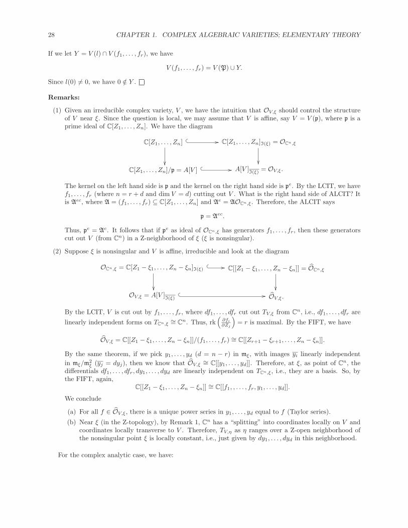
Remarks:
(1) Given an irreducible complex variety, V , we have the intuition that OV,ξ should control the structureof V near ξ. Since the question is local, we may assume that V is affine, say V = V (p), where p is aprime ideal of C[Z1, . . . , Zn]. We have the diagram
C[Z1, . . . , Zn]� � ��
��
C[Z1, . . . , Zn]I(ξ) = OCn,ξ
��C[Z1, . . . , Zn]/p = A[V ] � � �� A[V ]
I(ξ)= OV,ξ.
The kernel on the left hand side is p and the kernel on the right hand side is pe. By the LCIT, we havef1, . . . , fr (where n = r + d and dim V = d) cutting out V . What is the right hand side of ALCIT? Itis Aec, where A = (f1, . . . , fr) ⊆ C[Z1, . . . , Zn] and Ae = AOCn,ξ. Therefore, the ALCIT says
p = Aec.
Thus, pe = Ae. It follows that if pe as ideal of OCn,ξ has generators f1, . . . , fr, then these generatorscut out V (from C
n) in a Z-neighborhood of ξ (ξ is nonsingular).
(2) Suppose ξ is nonsingular and V is affine, irreducible and look at the diagram
OCn,ξ = C[Z1 − ξ1, . . . , Zn − ξn]I(ξ)� � ��
��
C[[Z1 − ξ1, . . . , Zn − ξn]] = OCn,ξ
��OV,ξ = A[V ]
I(ξ)� � �� OV,ξ.
By the LCIT, V is cut out by f1, . . . , fr, where df1, . . . , dfr cut out TV,ξ from Cn, i.e., df1, . . . , dfr are
linearly independent forms on TCn,ξ∼= C
n. Thus, rk(∂fi
∂Zj
)= r is maximal. By the FIFT, we have
OV,ξ = C[[Z1 − ξ1, . . . , Zn − ξn]]/(f1, . . . , fr) ∼= C[[Zr+1 − ξr+1, . . . , Zn − ξn]].
By the same theorem, if we pick y1, . . . , yd (d = n − r) in mξ, with images yi linearly independentin mξ/m
2ξ (yj = dyj), then we know that OV,ξ ∼= C[[y1, . . . , yd]]. Therefore, at ξ, as point of C
n, thedifferentials df1, . . . , dfr, dy1, . . . , dyd are linearly independent on TCn,ξ, i.e., they are a basis. So, bythe FIFT, again,
C[[Z1 − ξ1, . . . , Zn − ξn]] ∼= C[[f1, , . . . , fr, y1, . . . , yd]].
We conclude
(a) For all f ∈ OV,ξ, there is a unique power series in y1, . . . , yd equal to f (Taylor series).
(b) Near ξ (in the Z-topology), by Remark 1, Cn has a “splitting” into coordinates locally on V and
coordinates locally transverse to V . Therefore, TV,η as η ranges over a Z-open neighborhood ofthe nonsingular point ξ is locally constant, i.e., just given by dy1, . . . , dyd in this neighborhood.
For the complex analytic case, we have:
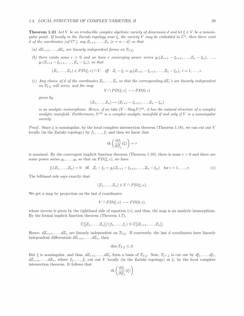
1.3. LOCAL STRUCTURE OF COMPLEX VARIETIES, II 29
Theorem 1.21 Let V be an irreducible complex algebraic variety of dimension d and let ξ ∈ V be a nonsin-gular point. If locally in the Zariski topology near ξ, the variety V may be embedded in C
n, then there existd of the coordinates (of C
n), say Zr+1, . . . , Zn (r = n− d) so that
(a) dZr+1, . . . , dZn are linearly independent forms on TV,ξ,
(b) there exists some ε > 0 and we have r converging power series g1(Zr+1 − ξr+1, . . . , Zn − ξn), . . .,gr(Zr+1 − ξr+1, . . . , Zn − ξn), so that
(Z1, . . . , Zn) ∈ PD(ξ, ε) ∩ V iff Zi − ξi = gi(Zr+1 − ξr+1, . . . , Zn − ξn), i = 1, . . . , r.
(c) Any choice of d of the coordinates Z1, . . . , Zn so that the corresponding dZi’s are linearly independenton TV,ξ will serve, and the map
V ∩ PD(ξ, ε) −→ PD(0, ε)
given by(Z1, . . . , Zn) �→ (Zr+1 − ξr+1, . . . , Zn − ξn)
is an analytic isomorphism. Hence, if we take (V −SingV )an, it has the natural structure of a complexanalytic manifold. Furthermore, V an is a complex analytic manifold if and only if V is a nonsingularvariety.
Proof . Since ξ is nonsingular, by the local complete intersection theorem (Theorem 1.18), we can cut out Vlocally (in the Zariski topology) by f1, . . . , fr and then we know that
rk(∂fi∂Zj
(ξ))
= r
is maximal. By the convergent implicit function theorem (Theorem 1.10), there is some ε > 0 and there aresome power series g1, . . . , gr so that on PD(ξ, ε), we have
fi(Z1, . . . , Zn) = 0 iff Zi − ξi = gi(Zr+1 − ξr+1, . . . , Zn − ξn) for i = 1, . . . , r. (∗)
The lefthand side says exactly that
(Z1, . . . , Zn) ∈ V ∩ PD(ξ, ε).
We get a map by projection on the last d coordinates
V ∩ PD(ξ, ε) −→ PD(0, ε),
whose inverse is given by the righthand side of equation (∗); and thus, the map is an analytic isomorphism.By the formal implicit function theorem (Theorem 1.7),
C[[Z1, . . . , Zn]]/(f1, . . . , fr) ∼= C[[Zr+1, . . . , Zn]].
Hence, dZr+1, . . . , dZn are linearly independent on TV,ξ. If conversely, the last d coordinates have linearlyindependent differentials dZr+1, . . . , dZn, then
dim TV,ξ ≤ d.
But ξ is nonsingular, and thus, dZr+1, . . . , dZn form a basis of TV,ξ. Now, TCn,ξ is cut out by df1, . . . , dfr,dZr+1, . . . , dZn, where f1, . . . , fr cut out V locally (in the Zariski topology) at ξ, by the local completeintersection theorem. It follows that
rk(∂fi∂Zj
(ξ))
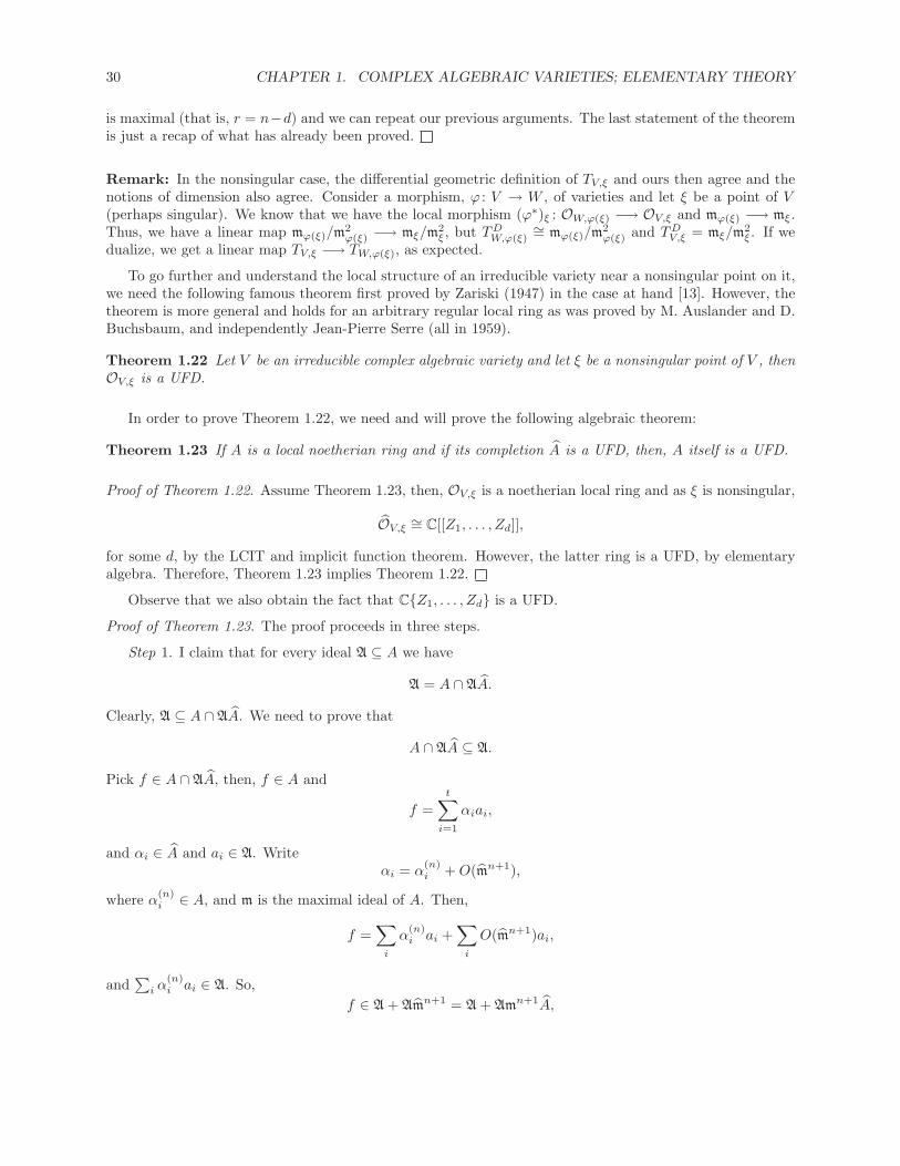
30 CHAPTER 1. COMPLEX ALGEBRAIC VARIETIES; ELEMENTARY THEORY
is maximal (that is, r = n−d) and we can repeat our previous arguments. The last statement of the theoremis just a recap of what has already been proved.
Remark: In the nonsingular case, the differential geometric definition of TV,ξ and ours then agree and thenotions of dimension also agree. Consider a morphism, ϕ : V → W , of varieties and let ξ be a point of V(perhaps singular). We know that we have the local morphism (ϕ∗)ξ : OW,ϕ(ξ) −→ OV,ξ and mϕ(ξ) −→ mξ.Thus, we have a linear map mϕ(ξ)/m
2ϕ(ξ) −→ mξ/m
2ξ , but TDW,ϕ(ξ)
∼= mϕ(ξ)/m2ϕ(ξ) and TDV,ξ = mξ/m
2ξ . If we
dualize, we get a linear map TV,ξ −→ TW,ϕ(ξ), as expected.
To go further and understand the local structure of an irreducible variety near a nonsingular point on it,we need the following famous theorem first proved by Zariski (1947) in the case at hand [13]. However, thetheorem is more general and holds for an arbitrary regular local ring as was proved by M. Auslander and D.Buchsbaum, and independently Jean-Pierre Serre (all in 1959).
Theorem 1.22 Let V be an irreducible complex algebraic variety and let ξ be a nonsingular point of V , thenOV,ξ is a UFD.
In order to prove Theorem 1.22, we need and will prove the following algebraic theorem:
Theorem 1.23 If A is a local noetherian ring and if its completion A is a UFD, then, A itself is a UFD.
Proof of Theorem 1.22. Assume Theorem 1.23, then, OV,ξ is a noetherian local ring and as ξ is nonsingular,
OV,ξ ∼= C[[Z1, . . . , Zd]],
for some d, by the LCIT and implicit function theorem. However, the latter ring is a UFD, by elementaryalgebra. Therefore, Theorem 1.23 implies Theorem 1.22.
Observe that we also obtain the fact that C{Z1, . . . , Zd} is a UFD.
Proof of Theorem 1.23. The proof proceeds in three steps.
Step 1. I claim that for every ideal A ⊆ A we have
A = A ∩ AA.
Clearly, A ⊆ A ∩ AA. We need to prove that
A ∩ AA ⊆ A.
Pick f ∈ A ∩ AA, then, f ∈ A and
f =t∑i=1
αiai,
and αi ∈ A and ai ∈ A. Writeαi = α
(n)i +O(mn+1),
where α(n)i ∈ A, and m is the maximal ideal of A. Then,
f =∑i
α(n)i ai +
∑i
O(mn+1)ai,
and∑i α
(n)i ai ∈ A. So,
f ∈ A + Amn+1 = A + Amn+1A,

1.3. LOCAL STRUCTURE OF COMPLEX VARIETIES, II 31
and this is true for all n. The piece of f in Amn+1A lies in A, and thus, in mn+1. We find that f ∈ A+mn+1
for all n, and we havef ∈
⋂n≥0
(A + mn+1) = A,
by Krull’s intersection theorem.
Step 2. I claim thatFrac(A) ∩ A = A.
This means that given f/g ∈ Frac(A) and f/g ∈ A, then f/g ∈ A. Equivalently, this means that if g dividesf in A, then g divides f in A. Look at
A = gA.
If f/g ∈ A, then f ∈ gA, and since f ∈ A, we have
f ∈ A ∩ gA.
But gA = AA, and by Step 1, we find that
gA = A = A ∩ AA,
so, f ∈ gA, as claimed.
We now come to the heart of the proof.
Step 3. Let f, g ∈ A with f irreducible. I claim that either f divides g in A or (f, g) = 1 in A (where(f, g) denotes the gcd of f and g).
Assuming this has been established, here is how we prove Theorem 1.23: Firstly, since A is noetherian,factorization into irreducible factors exists (but not necessarily uniquely). By elementary algebra, one knowsthat to prove uniqueness, it suffices to prove that if f is irreducible then f is prime. That is, if f is irreducibleand f divides gh, then we must prove either f divides g or f divides h.
If f divides g, then we are done. Otherwise, (f, g) = 1 in A, by Step 3. Now, f divides gh in A and A isa UFD, so that as (f, g) = 1 in A we find that f divides h in A. By Step 1 2, we get that f divides h in A,as desired.
Proof of Step 3. Let f, g ∈ A and let d be the gcd of f and g in A. Thus,
f = dF, and g = dG,
where d, F,G ∈ A, and(F,G) = 1 in A.
Let ordbm F = n0 (that is, n0 is characterized by the fact that F ∈ mn0 but F /∈ mn0+1). Either F is a unitor a nonunit in A. If F is a unit in A, then n0 = 0, and f = dF implies that F−1f = d; then,
F−1fG = g,
which implies that f divides g in A. By Step 2, we get that f divides g in A.
We now have to deal with the case where ord(F ) = n0 > 0. We have
F = limn→∞Fn and G = lim
n→∞Gn,
in the m-adic topology, with Fn and Gn ∈ A, and F − Fn and G−Gn ∈ mn+1. Look at
g
f− GnFn
=gFn − fGn
fFn.

32 CHAPTER 1. COMPLEX ALGEBRAIC VARIETIES; ELEMENTARY THEORY
Now,
gFn − fGn = g(Fn − F ) + gF − fGn= g(Fn − F ) + dGF − fGn= g(Fn − F ) + fG− fGn= g(Fn − F ) + f(G−Gn).
The righthand side belongs to (f, g)mn+1, which means that it belongs to (f, g)mn+1A. However, the lefthandside is in A, and thus, the righthand side belongs to
A ∩ (f, g)mn+1A.
Letting A = (f, g)mn+1, we can apply Step 1, and thus, the lefthand side belongs to (f, g)mn+1. This meansthat there are some σn, τn ∈ mn+1 ⊆ A so that
gFn − fGn = fσn + gτn;
It follows thatg(Fn − τn) = f(Gn + σn);
so, if we letαn = Gn + σn and βn = Fn − τn,
we have the following properties:
(1) gβn = fαn, with αn, βn ∈ A,
(2) αn ≡ Gn (mod mn+1) and βn ≡ Fn (mod mn+1),
(3) Gn ≡ G (mod mn+1A) and Fn ≡ F (mod mn+1A).
Choose n = n0. Since ord(F ) = n0 > 0, we have ord(Fn0) = n0, and thus, ord(βn0) = n0. Look at (1):
gβn0 = fαn0 ,
sodGβn0 = dFαn0 ,
and, because A is an integral domain,Gβn0 = Fαn0 .
However, (F,G) = 1 in A and F divides Gβn0 . Hence, F divides βn0 , so that there is some H ∈ A withβn0 = FH and
ord(βn0) = ord(F ) + ord(H).
But ord(F ) = n0, and consequently, ord(H) = 0, and H is a unit. Since βn0 = FH, we see that βn0 dividesF , and thus,
F = βn0δ
for some δ ∈ A. Again, ord(δ) = 0, and we conclude that δ is a unit. Then,
βn0δd = dF = f,
so that βn0 divides f in A. By step 2, βn0 divides f in A. But f is irreducible and βn0 is not a unit, and soβn0u = f where u is a unit. Thus, δd = u is a unit, and since δ is a unit, so is d, as desired.
The unique factorization theorem just proved has important consequences for the local structure of avariety near a nonsingular point:

1.3. LOCAL STRUCTURE OF COMPLEX VARIETIES, II 33
Theorem 1.24 Say V is an irreducible complex variety and let ξ be a point in V . Let f ∈ OV,ξ be a locallydefined holomorphic function at ξ and assume that f �≡ 0 on V and f(ξ) = 0. Then, the locally definedsubvariety, W = {x ∈ V | f(x) = 0}, given by f is a subvariety of codimension 1 in V . If ξ is nonsingularand f is irreducible, then W is irreducible. More generally, if ξ is nonsingular then the irreducible componentsof W through ξ correspond bijectively to the irreducible factors of f in OV,ξ. Conversely, suppose ξ isnonsingular and W is a locally defined pure codimension 1 subvariety of V through ξ, then, there is someirreducible f ∈ OV,ξ so that near enough ξ, we have
W = {x ∈ V | f(x) = 0} and I(W )OV,ξ = fOV,ξ.
Proof . Let ξ be a point in V and let f be in OV,ξ, with f irreducible. As the question is local on V we mayassume that V is affine. Also,
OV,ξ = lim−→g /∈I(ξ)
Ag,
with A = A[V ]. Thus, we may assume that f = F/G, with G(ξ) �= 0 and with F,G ∈ A. Upon replacing Vby VG (where VG is an open such that ξ ∈ VG), we may assume that f is the image of some F ∈ A = A[V ].The variety V is irreducible and V = V (p), where p is some prime ideal. Near ξ (i.e., on some open affinesubset U0 with ξ ∈ U0), let
A = {g ∈ C[Z1, . . . , Zn] | lg ∈ p + (f), where l(ξ) �= 0}, (∗)
and let m be the ideal of ξ on V . This means that m = {g ∈ A[V ] | g(ξ) = 0}. We have
p ⊆ A ⊆ m.
Reading the above in A, we get A ⊆ m, and in OV,ξ, we find from (∗) that Ae = fOV,ξ. Thus, Ae is aprime ideal, because f is irreducible and OV,ξ is a UFD. Then, A is prime and W = V (A) is a variety locallydefined by f = 0, and is irreducible. We have W �⊆ V , since f = 0 on W but not on V , and we find that
dim(W ) ≤ dim(V )− 1.
We will prove equality by a tangent space argument.
Claim. There is some affine open U ⊆ Wα with ξ ∈ U so that for all u ∈ U : TWα,u is cut out from TV,uby the equation df = 0, where Wα is some irreducible component of W through ξ.
Let g1, . . . , gt be generators for A. Thus, dg1 = · · · = dgt = 0 cut out TW,u near ξ, i.e., in some suitableopen set U0 with ξ ∈ U0. By (∗), on U0, there exist l1, . . . , lt so that
ligi = pi + λif,
where pi ∈ p, and the λi’s are polynomials. Let l =∏li, and take
U = U0 ∩ {η | l(η) �= 0}.
The set U is open and affine. By differentiating, we get
lidgi + (dli)gi = dpi + (dλi)f + λidf. (†)
On U ⊆W ⊆ V , we have
(1) f = 0 (in W ).
(2) pi = 0 (in V ).
(3) gi = 0 (in W ).
34 CHAPTER 1. COMPLEX ALGEBRAIC VARIETIES; ELEMENTARY THEORY
(4) li �= 0.
(5) dpi = 0, as we are in TV,u, with u ∈ U .
In view of (†), we getli(u)dgi(u) = λi(u)df(u).
Assume that df(u) = 0. Since li(u) �= 0, we get dgi(u) = 0, which implies that the equation df(u) = 0 cutsout a subspace of TW,u. Then, TW,u contains the hyperplane df = 0 of TV,u, which implies that
dim(TW,u) ≥ dim(TV,u)− 1.
Now, Z-open are dense in irreducible; consequently on some irreducible component Wα of W , U ∩Wα isopen, dense and some u in U ∩Wα is nonsingular, so
dimW ≥ dimWα = dim(TW,u) ≥ dim(TV,u)− 1 ≥ dim V − 1.
Thus, (by previous work),dim(W ) = dim(V )− 1.
Conversely, assume that W is locally defined near ξ, and is of codimension 1. Replacing V by this affineneighborhood, we may assume that W ⊆ V , is globally defined, and of codimension 1. Also recall that ξ isassumed to be nonsingular. We have the ideal I(W )OV,ξ in OV,ξ, and we can write
I(W )OV,ξ = p1 ∩ · · · ∩ pt,
where the pj ’s are minimal primes of OV,ξ, each of height 1. Since OV,ξ is a UFD, every pi is principal, i.e.,pi = fiOV,ξ, where fi is irreducible. As
p1 ∩ · · · ∩ pt = p1 · · · pt,
we getI(W )OV,ξ = fOV,ξ,
where f = f1 · · · ft. The above argument implies that I(W ) = (F ) in some AG, where A = A[V ]; G(ξ) �= 0;G ∈ A. Thus, I(W ) is locally principal. Observe also that if W is irreducible, then I(W ) is prime; so, f = fjfor some j, i.e., f is irreducible.
Now, consider f ∈ OV,ξ, where ξ is not necessarily nonsingular, and look at the local variety through ξdefined by f = 0 (remember, f(ξ) = 0). The radical ideal A = I(W ) (in A = C[Z1, . . . , Zn]/p) defining Whas a decomposition
A = p1 ∩ · · · ∩ pt,
and since A =√
A, the pj ’s are the minimal primes containing A (the isolated primes of A). Let g1, . . . , gt begenerators of A. The image of gj in OV,ξ has the form λjf (remember, W is locally principal by hypothesis).Since
OV,ξ = lim−→G/∈I(ξ)
AG,
take G enough for g1, . . . , gt, and then the open VG so that gj = λjF , where I(W ) in AG is just (F ), andF/G = f in OV,ξ. Thus,
A = I(W ) =s⋂j=1
pj ,
where in the above intersection, we find only the primes surviving in OV,ξ, i.e., those with pj ⊆ m, wherem = I(ξ). By Krull’s principal ideal theorem (Zariski and Samuel [14], Theorem 29, Chapter IV, Section14), these pj ’s are minimal ideals, and thus, the components of W have codimension 1.

1.3. LOCAL STRUCTURE OF COMPLEX VARIETIES, II 35
If ξ is actually nonsingular, then these surviving pj ’s are minimal in the UFD OV,ξ. Hence, locallyenough, each pj is principal; say pj = (fj). Then,
(f) = A = (f1) ∩ · · · ∩ (fs) = (f1 · · · fs);
so thatf = uf1 · · · fs
where u is a unit. The irreducible branches of W through ξ are the irreducible factors of the local equationf = 0 defining W locally.
Nomenclature: If V is a complex variety, then a Cartier divisor on V is a subvariety, W ⊆ V , so that forall ξ ∈W , there is Uξ open in V , with ξ ∈ Uξ and there is some function fξ locally defined on Uξ so that
W ∩ Uξ = {η | fξ(η) = 0}.
Then, the translation of Theorem 1.24 is:
Corollary 1.25 If V is a complex variety, then every Cartier divisor is a pure codimension one subvarietyof V . If ξ is nonsingular, then a pure codimension one subvariety of V through ξ is a Cartier divisor near ξ.
Corollary 1.26 (Hypersurface Intersection Theorem) Say V is a complex variety and f is a global function(f �≡ 0) on V . Let W = {v ∈ V | f(v) = 0} (e.g., V ⊆ C
N is affine, H = a hyperplane in CN given by
H = {x ∈ CN | F (x) = 0} and W = V ∩H, with V �⊆ H and V ∩H �= ∅.) If f �≡ 0 and f is not a unit,
then each irreducible component of W has codimension 1.
Corollary 1.27 (Intersection Dimension Theorem) Say V,W,Z are irreducible complex varieties andV,W ⊆ Z. Pick ξ ∈ V ∩W and assume ξ is a nonsingular point of Z. Then, V ∩W = (
⋃α Tα) ∪Q, where
(1) The Tα are irreducible components of V ∩W through ξ.
(2) Q = the rest of V ∩W .
(3) dim Tα ≥ dim V + dimW − dim Z, for all α.
Proof . (1) and (2) simply set up the notation and we just have to prove (3). We may assume that V,W,Z areaffine (by density of a Z-open in an irreducible), say Z ⊆ C
N . As ξ is nonsingular, if dim Z = n, there existfunctions g1, . . . , gn on Z with dg1, . . . , dgn a basis for TDZ,ξ (by the Local Complete Intersection Theorem).Observe that
V ∩W = (V∏
W ) ∩∆Z ,
where ∆Z ⊆ Z∏Z is the diagonal. Consider the functions f1, . . . , fn on Z
∏Z given (near ξ) by
fi(z1, . . . , zn;w1, . . . , wn) = gi(z1, . . . , zn)− gi(w1, . . . , wn), i = 1, . . . , n.
Clearly, fi � ∆Z ≡ 0 (near (ξ, ξ)) and df1, . . . , dfn are l.i. at (ξ, ξ) on the tangent space. By the LCIT, wemust have
C(f1, . . . , fn) = ∆Z ∪R,where R = the union of the irreducible components of V (f1, . . . , fn) through (ξ, ξ). Therefore, near ξ, wehave
V ∩W = (V ∩W ) ∩ V (f1) ∩ · · · ∩ V (fn).
By Corollary 1.26, dim Tα ≥ dim(V∏W )− n. However, dim(V
∏W ) = dim V + dimW , so
dim Tα ≥ dim V + dimW − dim Z.

36 CHAPTER 1. COMPLEX ALGEBRAIC VARIETIES; ELEMENTARY THEORY
� If V and W are contained in some affine variety Z not Cq, the intersection dimension theorem may be
false at a singular point. Indeed, consider the following example.
Example 1.2 Let Z be the quadric cone in C4 given by
x1x2 − x3x4 = 0.
The cone Z has dimension 3 (it is a hypersurface). Let V be the plane
x1 = x3 = 0,
and W the planex2 = x4 = 0.
Observe that V,W ⊆ Z. Since V and W have dimension 2 and V ∩W �= ∅, the intersection dimensiontheorem would yield dim(V ∩ W ) ≥ 2 + 2 − 3 = 1. However V ∩ W = {(0, 0, 0, 0)}, the origin, whosedimension is zero!
What is the problem? The answer is that near 0, ∆ ∩ Z is not the locus of three equations, but ratherof four equations.
Corollary 1.28 (Intersection Dimension Theorem in CN and P
N )
(1) Say V,W are complex affine varieties V,W ⊆ CN . Then, every irreducible component of V ∩W has
dimension at least dim V + dimW −N .
(2) Say V,W are complex varieties V,W ⊆ PN , with dim V + dimW ≥ N . Then, V ∩W �= ∅ and every
irreducible component of V ∩W has dimension at least dim V + dimW −N .
Proof . (1) As each point of CN is nonsingular, we can apply Corollary 1.28.
(2) Write C(V ), C(W ) for the cones over V and W in CN+1, i.e., the affine varieties given by the same
homogeneous equations regarded in affine space CN+1. We have dim C(V ) = dim V + 1 and
dim C(W ) = dimW + 1. As 0 ∈ C(V ) ∩ C(W ), by part (1), every irreducible component of C(V ) ∩ C(W )through 0 has dimension at least dim V + 1 + dimW + 1 − (N + 1), i.e., (dim V + dimW −N) + 1. But,each such irreducible component is the cone over the corresponding irreducible component of V ∩W and,as dim V + dimW ≥ N , we deduce that these irreducible affine cones have dimension at least 1, so that thecorresponding irreducible components in P
N are nonempty. The rest is clear.
1.4 Elementary Global Theory of Varieties
We begin by observing that the category of complex varieties has fibred products. The set-up is the following:V and W are two given varieties and we have two morphisms p : V → Z and q : W → Z, where W is anothercomplex variety. We seek a variety, P , together with two morphisms, pr1 : P → V and pr2 : P →W , so thatthe diagram below commutes
Ppr2 ��
pr1
��
W
q
��V p
�� Z
and so that for every test variety, T , and morphisms, ϕ : T → V and ψ : T →W , so that the diagram
Tψ ��
ϕ
��
W
q
��V p
�� Z

1.4. ELEMENTARY GLOBAL THEORY OF VARIETIES 37
commutes, there is a unique morphism, (ϕ,ψ) : T → P , with
ϕ = pr1 ◦ (ϕ,ψ) and ψ = pr2 ◦ (ϕ,ψ).
Such a variety, P , always exists and is unique up to (unique) isomorphism (use glueing, DX). This varietyis called the fibred product of V and W over Z and is denoted V
∏Z
W .
Say we have a morphism p : V → Z, and let z ∈ Z be any point in Z. Then {z} ⊆ Z is Z-closed, i.e.,the inclusion map, q : {z} → Z is a morphism. Consequently, we can make the fibred product V
∏Z
{z}, a
variety. Set theoretically, it is the fibre p−1(z).
Theorem 1.29 (Fibre Dimension Theorem) If ϕ : V → Z is a surjective morphism of complex, irreduciblevarieties, then
(1) For every z ∈ Z,dim ϕ−1(z) ≥ dim V − dim Z.
(2) There is a Z-open, U ⊆ Z, so that, for every u ∈ U ,
dim ϕ−1(u) = dim V − dim Z.
Proof . You check (DX), we may assume Z is affine, say Z ⊆ CN .
(1) Pick ξ ∈ Z, ξ �= z. There is a hyperplane H ⊆ CN such that z ∈ H and ξ /∈ H. Thus, Z is not
contained in H. [In fact, if L = 0 is a linear form defining H, Ld (d ≥ 1) is a form of degree d defining ahypersurface of degree d, call it H ′; Z is not contained in H ′, but z ∈ H ′.] By the hypersurface intersectiontheorem (Corollary 1.26), the dimension of any irreducible component of Z∩H is dim(Z)−1. Pick, ξ1, . . . ξsin each of the components of Z ∩H. Then, there is a hyperplane H so that ξj /∈ H for all j, 1 ≤ j ≤ s, butz ∈ H. Then, by Corollary 1.26 again, the dimension of any component of Z ∩H ∩ H is dim(Z)− 2. Usingthis process, we get some hyperplanes H = H1,H2, . . . , Hm such that
z ∈m⋂j=1
Hj ,
and if we writeZj = Zj−1 ∩Hj ,
with Z1 = Z ∩H1, we get a chain
Z ⊃ Z1 ⊃ Z2 ⊃ · · · ⊃ Zm with m = dim Z.
Here, z ∈ Zm, anddim(Zj) = dim(Z)− j.
Thus, the linear forms L1, . . . , Lm associated with the Hj ’s define Zm in Z and
dim(Zm) = 0.
Consequently, Zm is a finite set of points:
Zm = {z = z1, z2, . . . , zt}.
LetU0 = Z − {z2, . . . , zt},
38 CHAPTER 1. COMPLEX ALGEBRAIC VARIETIES; ELEMENTARY THEORY
it is a Z-open dense subset of Z. We can replace Z by U0, and thus, we may assume that Zm = {z}. Wehave the morphism ϕ : V → Z, and so, each ϕ∗(Lj) is a global function on V (where ϕ∗ : ϕ∗OZ → OV ). Butthen, ϕ−1(z) is the locus in V cut out by ϕ∗(L1), . . . , ϕ∗(Lm); so, by the intersection dimension theorem,we get
dim ϕ−1(z) ≥ dim(V )−m = dim(V )− dim Z.
(2) We need to prove that there is a Z-open, U ⊆ Z, so that dimϕ−1(u) = dim V − dimZ, for all u ∈ U .As this statement is local on the base, we may assume that Z is affine. Assume at first that V is affine as well.By hypothesis, ϕ : V → Z is onto (ϕ(V ) Z-dense in Z is enough), so the corresponding map A[Z] −→ A[V ]is an injection (DX). If we let m = dim Z and n = dim V , as tr.dC A[Z] = m and tr.dC A[V ] = n, we have
tr.dA[Z]A[V ] = n−m.
Now, we have V ↪→ CN , with A[V ] = C[v1, . . . , vN ] and Z ↪→ C
M , with A[Z] = C[z1, . . . , zM ], for someM,N . We can choose and reorder the vj ’s so that v1, . . . , vn−m form a transcendence basis of A[V ] overA[Z]. Then, each vj (j = n−m+ 1, . . . , N) is algebraic over A[Z][v1, . . . , vn−m], and there are polynomialsGj(T1, . . . , Tn−m, T ) (coefficients in A[Z]) so that
Gj(v1, . . . , vn−m, vj) = 0.
Pick gj(T1, . . . , Tn−m) as the coefficient of highest degree of Gj in T . The set
{z ∈ Z | gj(z) = 0} = Zj
is a Z-closed subset of Z. Let
U = Z −N⋃
j=n−m+1
Zj .
The Z-open U is nonempty, since Z is irreducible. On U , the polynomial Gj is not identically zero as apolynomial in T1, . . . , Tn−m, T , yet
Gj(v1, . . . , vn−m, vj) = 0.
Thus, vj is algebraically dependent on v1, . . . , vn−m over A[U ]. Letting vj denote the restriction of vj toϕ−1(z) (i.e., the image of vj in A[V ] ⊗A[Z] C), where z ∈ U , we see that vj is also algebraically dependenton v1, . . ., vn−m. Now,
A[ϕ−1(z)] = C[v1, . . . , vn−m] = A[V ]⊗A[Z] C,
which implies thatdim(ϕ−1(z)) = tr.dC C[v1, . . . , vn−m] ≤ n−m.
However, by (1),dim(ϕ−1(z)) ≥ n−m,
and so, dim(ϕ−1(z)) = n−m on U .
If V is not affine, cover V by affine opens, Vα; each Vα is Z-dense in V (since V is irred.) Then, for everyz ∈ Z, we have ϕ−1(z) =
⋃α(Vα∩ϕ−1(z)) =
⋃α ϕ
−1α (z). Here, ϕα : Vα ↪→ V
ϕ−→ Z. Now, ϕα(Vα) is Z-densein Z, so the above implies that there exist some opens Uα in Z so that dim ϕ−1
α (z) = n−m if z ∈ Uα. Wecan take U =
⋂α Uα (a finite intersection since Z is a variety, and thus, is quasi-compact).
Corollary 1.30 Assume that we are in the same situation as in the fibre dimension theorem. Let
Zl = {w ∈ Z | dim(ϕ−1(w)) ≥ l}.
Then, Zl is Z-closed in Z, i.e., the function
w �→ dim(ϕ−1(w))

1.4. ELEMENTARY GLOBAL THEORY OF VARIETIES 39
is upper semi-continuous on Z. Hence, Z possesses a stratification
Z = U0 ∪ U1 ∪ · · · ∪ Un,
where Uj = Zj − Zj+1 = {z ∈ Z | dim ϕ−1(z) = l} is locally closed and dim(ϕ−1(w)) = j for all w ∈ Uj.
Proof . The proof is by induction on dim(Z). The case where dim(Z) = 0 is easy. Given Z, Theorem 1.29part (2) implies that there is some open set U ⊆ Z and some Zl (l ≥ 1 and l minimum) so that
Zl ⊆ Z = Z − U.
Also, Z is closed and we have some irredundant decomposition
Z =t⋃
j=1
Zj ,
where Zj is irreducible and strictly contained in Z. Then, dim(Zj) < dim(Z), and we can apply the inductionhypothesis to the maps ϕj : ϕ−1(Zj)→ Zj , the details are left as an exercise (DX).
Observe that given a morphism ϕ : V → Z, we can write
V =⋃z∈Z
ϕ−1(z).
Each ϕ−1(z) is a complex algebraic variety and these are indexed by an algebraic variety. Therefore, V isan algebraic family of varieties.
� Note that the dimension of the fibres may jump, as shown by the following example (which is nothingbut the “blowing-up” at a point in C
2).
Example 1.3 Let Z = C2, and consider C
2∏
P1. We use z1, z2 as cooordinates on Z, and ξ1, ξ2 as
homogeneous coordinates on P1. Write B0(C2) for the subvariety of C
2∏
P1 given by the equation
z1ξ2 = z2ξ1.
This equation is homogeneous in ξ1, ξ2, and it defines a closed subvariety of C2∏
P1. We get a morphism
ϕ : B0(C2)→ Z viaϕ : B0(C2) ↪→ C
2∏
P1 pr1−→ Z = C
2.
If z = (z1, z2) �= (0, 0), then the fibre over z is {(ξ1 : ξ2) | z1ξ2 = z2ξ1}.
1. If z1 �= 0, then ξ2 = (z2/z1)ξ1.
2. If z2 �= 0, then ξ1 = (z1/z2)ξ2.
In both cases, we get a single point (z1, z2; (1 : z2/z1)) in case (1) and (z1, z2; (z1/z2 : 1)) in case (2)) andthe dimension of the fibre ϕ−1(z) is zero for z ∈ C− {(0, 0)}. In fact, observe that
B0(C2)− pr−11 ((0, 0))
pr1
−→ C2 − {(0, 0)}.
Therefore, pr1 is a birational morphism between B0(C2) and C2. Observe that pr2 : B0(C2) → P
1 is alsosurjective and the fibre over every point of P
1 is a line. It turns out that B0(C2) is a line bundle over P1.
When z = (0, 0), the fibre is the whole P1. Thus, the dimension of the fibre at the origin jumps from 0
to 1.
40 CHAPTER 1. COMPLEX ALGEBRAIC VARIETIES; ELEMENTARY THEORY
In algebraic geometry, we have the analog of the notions of being Hausdorff or compact, but here workingfor the Zariski topology.
Definition 1.6 A morphism ϕ : V → W is separated iff ∆WV = the diagonal in V∏W
V is Z-closed in
V∏W
V . A variety, V , is separated when the morphism V −→ ∗ is separated, where ∗ is any one-point
variety.
Examples of separated varieties.
(1) Any affine variety and any projective variety is separated.
(2) Any closed or open subvariety of a separated variety is separated (DX).
(3) We say that V is quasi-affine (resp. quasi-projective) iff it is open in an affine (resp. open in aprojective) variety. These are separated.
(4) The product of separated varieties is separated.
(5) The variety we get from two copies of P1 by glueing the opens C
1 − {0} by the identity map is notseparated.
Definition 1.7 A morphism, ϕ : V →W , is proper iff
(a) It is separated and
(b) For every variety, T , the second projection map, pr2 : V∏W
T → T , is a Z-closed morphism.
We say that a variety, V , is proper iff it is separated and if property (b) holds (W = {∗}).
As we said, the notion of properness of a variety is the algebraic substitute for compactness. An olderterminology is the term complete variety . As an illustration of the similarity of properness and compactness,we have the following property (well known for continuous maps on compact spaces):
Proposition 1.31 If V is proper and W is separated, then any morphism ϕ : V →W is Z-closed.
Proof . Consider the graph morphismΓϕ : V → V
∏W,
given byΓϕ(v) = (v, ϕ(v)).
Note that the image of Γϕ is closed in V∏W because W is separated. Indeed, consider the morphism
(ϕ, id) : V∏
W →W∏
W
given by(ϕ, id)(v, w) = (ϕ(v), w).
It is obvious that Im Γϕ = (ϕ, id)−1(∆W ), where ∆W is the diagonal in W∏W . But, W is separated, so
∆W is Z-closed in W∏W and consequently, (ϕ, id)−1(∆W ) is Z-closed in V
∏W . Since V is proper, by
setting T = W in condition (b), we see that pr2 : V∏W → W is Z-closed and so, pr2(Im Γϕ) is Z-closed
in W . However, pr2(Im Γϕ) = Im ϕ, therefore, Im ϕ is closed. If C is closed in V , then the compositionC ↪→ V −→ ∗ is proper (DX). Replace V by C and apply the above argument to get Im C is closed.
1.4. ELEMENTARY GLOBAL THEORY OF VARIETIES 41
Theorem 1.32 (Properness of projective varieties) A projective variety, V , is a proper variety. This meansthat for every variety W ,
pr2 : V∏
W −→W
is a Z-closed map.
Proof . (1) We reduce the proof to the case where W is affine. Assume that the theorem holds when W isaffine. Cover W with affine opens Wα, so that W =
⋃αWα. Check that
V∏
W ∼=⋃α
(V∏
Wα
).
Let C ⊆ V∏W be a closed subvariety. If Cα denotes C ∩ (V
∏Wα), then,
pr2(C) ∩Wα = pr2(Cα).
But, pr2(Cα) is closed in Wα, which implies that pr2(C) is closed in W .
(2) We reduce the proof to the case where V = Pn. Assume that the theorem holds for P
n. We have aclosed immersion, V ↪→ P
n, soV∏
W ↪→ Pn∏
W
is also a closed immersion (= embedding) (DX). Hence, we have the commutative diagram
C� � �� V
∏W
pr2 �����
����
��
� � �� Pn∏nW
pr2�������
����
W
,
and this shows that we may assume that V = Pn.
(3) Lastly, we reduce the proof to the case: W = Cm. Assume that the theorem holds for W = C
m. By(1), we may assume that W is closed in C
m, then we have the following commutative diagram:
C� � �� P
n∏W
(pr2)W
��
� � �� Pn∏
Cm
(pr2)Cm
��W
� � �� Cm
where the arrows in the top line are closed immersions (for the second arrow, this is because W ↪→ Cm, as
in (2)). So,(pr2)W (C) = (pr2)Cm(C) ∩W,
and, since by hypothesis, (pr2)Cm(C) is closed, and W is closed, we find (pr2)W (C) is also closed.
We are now reduced to the essential case: Which is to prove that pr2 : Pn∏
Cm → C
m is a closed map.
Let C be a closed subvariety of Pn∏
Cm. Then, C is the common solution set of a system of equations of
form
fj(X0, . . . , Xn;Y1, . . . , Ym) = 0, for j = 1, . . . , p, (†)
42 CHAPTER 1. COMPLEX ALGEBRAIC VARIETIES; ELEMENTARY THEORY
where fj is homogeneous in the Xj ’s and we restrict to solutions for which Xj �= 0 for some j, with 0 ≤ j ≤ n.Pick y ∈ C
m, and write y = (y1, . . . , ym); also write (†)(y) for the system (†) in which we have set Yj = yjfor j = 1, . . . ,m.
Plan of the proof : We will prove that (pr2(C))c (the complement of pr2(C)) is open. Observe that
y ∈ pr2(C) iff (∃x)((x, y) ∈ C)iff (∃x)(xj �= 0 for some j, and (†)(y) holds).
Thus,y ∈ (pr2(C))c iff (∀x)(if (†)(y) holds, then xj = 0, for 0 ≤ j ≤ n).
Let A(y) be the ideal generated by the polynomials, fj(X0, . . . , Xn, y1, . . . , ym), occurring in (†)(y). Hence,
y ∈ (pr2(C))c iff (∃d ≥ 0)((X0, . . . , Xn)d ⊆ A(y)).
LetNd = {y ∈ C
m | (X0, . . . , Xn)d ⊆ A(y)}.Then,
(pr2(C))c =∞⋃d=1
Nd.
Now,Nd ⊆ Nd+1,
and so,
(pr2(C))c =∞⋃
d>>0
Nd,
where d >> 0 means that d is sufficiently large.
Claim. If d > max{d1, . . . , dp}, where dj is the homogeneous degree of fj(X0, . . . , Xn, Y1, . . . , Ym) in theXi’s, then Nd is open in C
m. This will finish the proof.
Write Sd(y) for the vector space (over C) of polynomials in k[y1, . . . , ym][X0, . . . , Xn] of exact degree d.We have a map of vector spaces
ψd(y) : Sd−d1(y)⊕ · · · ⊕ Sd−dp(y) −→ Sd(y)
given by
ψd(y)(g1, . . . , gp) =p∑j=1
fj(X0, . . . , Xn, y1, . . . , ym)gj .
If we assume that ψd(y) is surjective, then all monomials of degree d are in the range of ψd(y). Thus, A(y)will contain all the generators of (X0, . . . , Xn)d, i.e.,
(X0, . . . , Xn)d ⊆ A(y),
and this meansy ∈ Nd.
Conversely, if y ∈ Nd, then (X0, . . . , Xn)d ⊆ A(y), and thus, A(y) contains every monomial of degree d. Butthen, each monomial of degree d is in the range of ψd(y), and since these monomials form a basis of Sd(y),the map ψd(y) is surjective.
Therefore, y ∈ Nd iff ψd(y) is surjective.

1.4. ELEMENTARY GLOBAL THEORY OF VARIETIES 43
Pick bases for all of the Sd−dj’s and for Sd. Then, ψd(Y ) is given by a matrix whose entries are polynomials
in the Yj ’s. We know that ψd(y) is surjective iff rkψd(y) = nd, where nd = dim(Sd)(y). Therefore, ψd(y) willbe surjective iff some nd × nd minor of our matrix is nonsingular. This holds if and only if the determinantof this minor is nonzero. However, these determinants for ψd(y) are polynomials q(Y1, . . . , Ym). Therefore,ψd(y) will be surjective iff y belongs to the Z-open such that some q(y) �= 0. This proves that Nd is open,and finishes the proof.
Remark: Homogeneity in the Xi’s allowed us to control degrees.
Corollary 1.33 Let V be a proper variety (e.g., by Theorem 1.32, any projective variety). If W is anyquasi-affine variety (i.e., an open in an affine) or any affine variety, then for any morphism ϕ : V → W ,the image, Im ϕ, of ϕ is a finite set of points. If V is Z-connected (e.g, norm connected or Z-connected),then ϕ is constant. In particular, every holomorphic function on V has finitely many values and if V isZ-connected, ϕ is constant.
Proof . Since Cn is separated, W is separated. We have
V −→W ↪→ Cn,
and thus, we may assume that W = Cn. Pick j, with 1 ≤ j ≤ n, and look at
V −→ Cn prj−→ C
1.
If we knew the result for C1, by a simple combinatorial argument, we would have the result for C
n. Thus,we are reduced to the case W = C
1. In this case, either Im ϕ = C1, or a finite set of points, since C
1 isirreducible. Furthermore, in the latter case, if V is Z-connected, then Im ϕ consists of a single point. Weneed to prove that ϕ : V → C
1 is never surjective. Assume it is. Consider the diagram
V∏
C1 ϕ
Qid ��
pr2����������
C1∏
C1
π2
��C
1
and letH = {(x, y) ∈ C
1 × C1 | xy = 1}.
The map ϕ∏
id is onto. Therefore, (ϕ∏
id)−1(H) is closed and
ϕ∏
id : (ϕ∏
id)−1(H)→ H
is surjective. Let C = (ϕ∏
id)−1(H). By the definition of proper, pr2(C) is closed. However, by commuta-tivity of the diagram,
pr2(C) = π2(H),
and yet, π2(H) = C1 − {0} is Z-open, a contradiction on the properness of C
1.
Corollary 1.34 (Kronecker’s main theorem of elimination) Consider p polynomialsf1(X0, . . . , Xn; Y1, . . . , Ym), . . ., fp(X0, . . . , Xn;Y1, . . . , Ym), with coefficients in C and homogeneous in theXi’s (of varying degrees). Consider further the simultaneous system
fj(X0, . . . , Xn;Y1, . . . , Ym) = 0, for j = 1, . . . , p. (†)
Then, there exist polynomials g1(Y1, . . . , Ym), . . ., gt(Y1, . . . , Ym) with coefficients in C involving only the Yj’sso that (†) has a solution in which not all Xi’s are 0 iff the system
gj(Y1, . . . , Yn) = 0, for j = 1, . . . , t, (††)
has a solution. (The Xi’s have been eliminated).

44 CHAPTER 1. COMPLEX ALGEBRAIC VARIETIES; ELEMENTARY THEORY
Proof . The system (†) defines a closed subvariety C of Pn∏
Cm.
Claim. The set pr2(C), which, by Theorem 1.32, is closed in Cm, gives us the system (††) by taking the
gj ’s as a set of polynomials defining pr2(C). To see this, note that C = ∅ iff pr2(C) = ∅; note further that(x, y) ∈ C iff (†) has a solution with not all Xi’s all zero. Consequently, (†) has a solution with not all Xi
zero iff (††) has a solution in the Yj ’s.
Theorem 1.35 (Irreducibility criterion) Say ϕ : V → W a surjective morphism with W separated andassume that
(1) V is proper
(2) W is irreducible.
(3) ϕ−1(w) is irreducible for every w ∈W .
(4) dim(ϕ−1(w)) = d, a constant for all w ∈W .
Then, V is irreducible.
Proof . Let V =⋃qj=1 Vj be an irredundant decomposition of V into irreducible components. Consider Vj .
It is closed in V , and thus, ϕ(Vj) is closed in W , because V is proper and W is separated. Since ϕ : V →Wis surjective,
W =q⋃j=1
ϕ(Vj).
But W is irreducible; so, it follows (after renumbering, if needed) that ϕ(Vj) = W for j = 1, . . . , s, and ϕ(Vj)is strictly contained in W for j = s+ 1, . . . , q. Thus,
q⋃j=s+1
ϕ(Vj)
is a Z-closed subset of W strictly contained in W , and
W = W −q⋃
j=s+1
ϕ(Vj)
is a Z-open dense subset of W , as W is irreducible. Let V = ϕ−1(W ), write Vj = V ∩ Vj , and let ϕj be therestriction of ϕ to Vj . Note,
ϕj(Vj) = ϕ(Vj) = W (1 ≤ j ≤ s),
because, given any w ∈ W , there exists v ∈ Vj with ϕ(v) = w. Since ϕ(v) ∈ W , the element v is in V .Therefore, v ∈ V ∩ Vj ; hence, v ∈ Vj , as required. Write
µj = min{dim(ϕ−1j (w)) | w ∈ W}.
By the fibre dimension theorem (Theorem 1.29), there is some nonempty open subset Uj ⊆ W so that ifw ∈ Uj , then dim(ϕ−1
j (w)) = µj . Thus, as U =⋂sj=1 Uj is a dense Z-open subset of W , we have a nontrivial
Z-dense open, U , so that if w ∈ U , then dim(ϕ−1j (w)) = µj , for j = 1, . . . , s. Pick w0 ∈ U . Then
ϕ−1(w0) =s⋃j=1
ϕ−1j (w0).

1.4. ELEMENTARY GLOBAL THEORY OF VARIETIES 45
However, ϕ−1(w0) is irreducible, and thus, there is some j such that
ϕ−1(w0) = ϕ−1j (w0).
We may assume that j = 1. Since the dimension of the fibres is constant, we get
µ1 = d.
By the fibre dimension theorem, dim ϕ−11 (w) ≥ dim ϕ−1
1 (w0) = d, for all w ∈W . Now,
ϕ−1(w) =s⋃j=1
ϕ−1j (w), (∗)
and since dim ϕ−11 (w) ≤ dim ϕ−1(w) = d, we must have dim ϕ−1
1 (w) = d for all w ∈ W and (∗) togetherwith the irreducibility of ϕ−1(w) imply that ϕ−1(w) = ϕ−1
1 (w), for all w ∈W . It follows that
V =⋃w∈W
ϕ−1(w) =⋃w∈W
ϕ−11 (w) = V1
and since V1 is irreducible, so is V .
� The conditions of the irreducibilty criterion though sufficient are not necessary. For example, takeπ : B0(Cn) → C
n. Outside 0 and π−1(0) we have an isomorphism and so, B0(Cn) is irreducible (itcontains a dense open which is irreducible), yet the fibres don’t have constant dimension.
Generally, given a morphism, ϕ : V →W , of algebraic varieties, the image, ϕ(Z), of a closed subset of Uis not closed. Nevertheless, it is natural to ask what kind of set ϕ(Z) is. The answer is given by a theoremof Chevalley and involves sets called constructible.
Definition 1.8 Given a topological space (for example, an affine variety) V , we say that a set Z is locallyclosed in V if
Z = U ∩W
where U is open and W is closed.
Observe that open and closed sets in a variety are locally closed. Let Zi = Ui ∩Wi, i = 1, 2. Then,
Z1 ∩ Z2 = U1 ∩ U2 ∩W1 ∩W2,
so that Z1 ∩ Z2 is locally closed. Thus, any finite intersection of locally closed sets is locally closed.
If Z = U ∩W , then Zc = U c ∪W c, where U c is closed and W c is open. It follows that the Booleanalgebra generated by the open and closed sets is just the set of finite unions of locally closed sets, denotedConstr(V ). Finite unions of locally closed sets are called constructible sets. We have the following importanttheorem.
Theorem 1.36 (Chevalley) If ϕ : V → W is a morphism of complex varieties and Z is a constructible setin V , then ϕ(Z) is constructible in W . If ϕ is dominant (i.e, ϕ(V ) = W ), then there is a nonempty open,U ⊆W , so that U ⊆ ϕ(V ) ⊆W .
Proof . Consider the statements
(1) The image of a constructible set in V is a constructible set in W .

46 CHAPTER 1. COMPLEX ALGEBRAIC VARIETIES; ELEMENTARY THEORY
(2) If ϕ(V ) is dense in W , there is some nonempty Z-open set U in W so that
U ⊆ ϕ(V ) ⊆W.
We first prove (2). I claim that (2) follows from the case where both V and W are irreducible. Let V ′ beany irreducible component of V . Then, ϕ(V ′) is irreducible in W , and thus, W = ϕ(V ′) is again irreducibleand closed in W . Let
W =t⋃
j=1
Wj ,
where the Wj are the irredundant components of W . Then
W =t⋃
j=1
W ∩Wj ,
and since W is irreducible, there is some j, 1 ≤ j ≤ t, such that W = W ∩Wj , i.e.,
W ⊆Wj .
But, if
V =s⋃i=1
Vi
is an irredundant decomposition of V , we showed that for every i, 1 ≤ i ≤ s, there is some j = j(i) so that
ϕ(Vi) ⊆Wj(i).
However,
ϕ(V ) = ϕ
(s⋃i=1
Vi
)=
s⋃i=1
ϕ(Vi).
Therefore,
W = ϕ(V ) =s⋃i=1
ϕ(Vi) =s⋃i=1
ϕ(Vi) ⊆s⋃i=1
Wj(i) =s⋃i=1
Wj(i) ⊆t⋃
j=1
Wj = W,
and the inclusions are all equalities. Since the decompositions are irredundant, the Wj(i) run over all theWj ’s and, by denseness, ϕ(Vi) is dense in Wj(i).
Assume that the theorem (2) holds when V is irreducible (so is W , since W = ϕ(V )). Then, for every i,there is some Z-open subset Ui ⊆Wj(i) so that
Ui ⊆ ϕ(Vi) ⊆Wj(i).
If Ci = Wj(i) − Ui, then Ci is closed in Wj(i), which implies that Ci is closed in W . The image ϕ(V ) missesat most
C =s⋃i=1
Ci,
which is closed. Therefore, U = Cc is a nonempty Z-open contained in ϕ(V ). Therefore, we may assumethat V and W are irreducible.
I now claim that we may also assume that V and W are affine. Since W is affine, we have W =⋃αWα
for some affine Z-open sets Wα. Let Vα = ϕ−1(Vα). Note that Wα is Z-dense in W and Vα is Z-dense in V .Thus, if V 0
α is open and Z-dense in Vα, then V 0α is also Z-dense in V . Let V 0
α be an affine open in Vα, then
1.4. ELEMENTARY GLOBAL THEORY OF VARIETIES 47
(i) V 0α ,Wα are affine.
(ii) V 0α ,Wα are irreducible.
(iii) ϕ(V 0α ) = Wα.
Then, there is some open subset Uα of Wα so that
Uα ⊆ ϕ(V 0α ) ⊆ ϕ(Vα) ⊆ ϕ(V ) ⊆W,
and Uα is open in W (as an open in an open).
We are finally reduced to the basic case: V and W are irreducible, affine and ϕ is dominant.
As ϕ(V ) is Z-dense in W , we know that A[W ] ↪→ A[V ] is an inclusion. Letting r = tr.dA[W ]A[V ], we picksome transcendence base ξ1, . . . , ξr (ξj ∈ A[V ]) over A[W ], so that A[V ] is algebraic over A[W ][ξ1, . . . , ξr].Since
A[W ][ξ1, . . . , ξr] ∼= A[W ]⊗C C[ξ1, . . . , ξr],
the map
A[W ] ↪→ A[W ][ξ1, . . . , ξr] ↪→ A[V ] (∗)
is just the mapϕ : A[W ] ↪→ A[W ]⊗C A[ξ1, . . . , ξr] ↪→ A[V ].
Reading the above geometrically, we get the map
ϕ : Vϕ1−→W
∏Cr pr1−→W.
Since each η ∈ A[V ] is algebraic over A[W∏
Cr], we have equations
a0(ξ1, . . . , ξr)ηs + a1(ξ1, . . . , ξr)ηs−1 + · · ·+ as(ξ1, . . . , ξr) = 0,
where the coefficients aj(ξ1, . . . , ξr) are functions over W , and thus, depend on w ∈ W , but we omit w forsimplicity of notation. If we multiply by a0(ξ1, . . . , ξr)s−1 and let ζ = a0(ξ1, . . . , ξr)η, we get
ζs + b1(ξ1, . . . , ξr)ζs−1 + · · ·+ bs(ξ1, . . . , ξr) = 0.
Therefore, for every η ∈ A[V ], there is some α ∈ A[W∏
Cr] so that
ζ = αη
is integral over A[W∏
Cr]. Since A[V ] is finitely generated, there exist η1, . . . , ηt so that
A[V ] = A[W∏
Cr][η1, . . . , ηt],
and each ηj comes with its corresponding αj and αjηj is integral over A[W∏
Cr]. Let
b =t∏
j=1
αj(ξ1, . . . , ξs) ∈ A[W∏
Cr].
Let U1 be the Z-open of W∏
Cr where b is invertible; it is that affine variety in W
∏Cr whose coordinate
ring is A[W∏
Cr]b. We have U1 ⊆ W
∏Cr, and on U1, b and all the αj ’s are invertible. Let us look
at b = ϕ1(b) ∈ A[V ], where ϕ1 : A[W∏
Cr] → A[V ] is the algebra homomorphism associated with the
morphism ϕ1 : V →W∏
Cr. Then, we get
Vbbϕ1−→ U1.

48 CHAPTER 1. COMPLEX ALGEBRAIC VARIETIES; ELEMENTARY THEORY
Since each αj is invertible, on Vbb, each ηj is integral over A[U1]. But Vbb is generated by the ηj ’s; so Vbb isintegral over U1. And therefore, the image of the morphism
Vbbϕ1−→ U1 (†)
is closed (DX). Consequently, as Vbb −→ U1 has dense image, (†) is a surjection of varieties, and we find
U1 = ϕ1(Vbb) ⊆ ϕ1(V ) ⊆W∏
Cr.
Even though U1 is a nonempty open, we still need to show that there is some nonempty open U ⊆ W suchthat U ⊆ pr1(U1). For then, we will have U ⊆ ϕ(V ). Now, b ∈ A[W
∏Cr] means that b can be expressed
by a formula of the formb =
∑(β)
b(β)(w)ξ(β),
where (β) denotes the multi-index (β) = (β1, . . . , βr), x(β) = ξβ11 · · · ξβr
r , and b(β) ∈ A[W ]. Let
U = {w ∈W | ∃(β), b(β)(w) �= 0}.
The set U is a Z-open set in W . If w ∈ U , since b is a polynomial in the ξj ’s which is not identically null, thereis some (β) such that b(β)(w) �= 0. Now, C is infinite, so there are some elements t1, . . . , tr ∈ C such thatb(w, t1, . . . , tr) �= 0. However, (w, t1, . . . , tr) ∈ W
∏Cr and b(w, t1, . . . , tr) �= 0, so that (w, t1, . . . , tr) ∈ U1
and pr1(w, t1, . . . , tr) = w. Therefore, U ⊆ pr1(U1), which concludes the proof of (2).
(1) Say Z is constructible in V , then
Z = (U1 ∩ V1) ∪ · · · ∪ (Un ∩ Vn),
where each Ui ⊆ V is open and each Vi ⊆ V is closed. Since ϕ(Z) =⋃nj=1 ϕ(Ui ∩ Uj), we may assume that
Z is locally closed.
Say we know that ϕ(Z) is constructible if Z is a variety and further, U open (in a variety) implies ϕ(U)is constructible. Take Z locally closed in V , then
Z = U1 ∩ V1 ↪→ V1 ↪→ Vϕ−→W,
and if we let ϕ1 be the composition V1 ↪→ Vϕ−→ W , then ϕ1 is a morphism. As Z is open in V1, by
assumption, ϕ1(Z) = ϕ(Z) is constructible in W .
Now, assume that ϕ(V ) is constructible if V is an affine variety. Take U , any open in V . Since V isa variety, we can write V =
⋃α Vα, where each Vα is affine open. Then, U =
⋃α(U ∩ Vα) and ϕ(U) =⋃
α ϕ(U ∩ Vα), where each U ∩ Vα is open in an affine. Consequently, we may assume that U is open in anaffine. In this case,
U = Vf1 ∪ · · · ∪ Vfl,
a union of affine varieties and
ϕ(U) =l⋃
j=1
ϕ(Vfj),
a union of constructible as each Vfjis an affine variety. Therefore, we are reduced to the case where Z is an
affine variety and we have to prove that ϕ(Z) is constructible.
I claim that we can assume that ϕ(V ) is Z-dense in W . For, Let W = Im ϕ. If Im ϕ is constructible inW , then
Im ϕ = U1 ∩ W1 ∪ . . . ∪ Un ∩ Wn,

1.4. ELEMENTARY GLOBAL THEORY OF VARIETIES 49
where Uj is open in W , and Wj is closed in W , which implies that Wj is closed in W . By definition of therelative topology, there are some open sets U ′
j in W so that
W ∩ U ′j = Uj .
Then, we have
Im ϕ = (W ∩ U ′1) ∩ W1 ∪ · · · ∪ (W ∩ U ′
n) ∩ Wn
= W ∩ (U ′1 ∩ W1 ∪ · · · ∪ U ′
n ∩ Wn)
= U ′1 ∩ W1 ∪ · · · ∪ U ′
n ∩ Wn,
a constructible set in W . As a consequence, we may assume that W = W , i.e., that Im ϕ is dense in W .Now, as ϕ(V ) is dense in W and V is irreducible, it follows that W is also irreducible and we can finish theproof by induction on dim V .
If dim V = 0, then both V and ϕ(V ) consist of a single point and (1) holds trivially.
Assume the induction hypothesis holds if dim V = r − 1 and let dim V = r. By (2), there is somenonempty open subset U of W such that U ⊆ ϕ(V ). Let T = ϕ−1(U). This is a Z-open subset of V andmoreover, ϕ(T ) = U . Let Z = V − T . The set Z is Z-closed in V , and thus
dim Z < dim V,
and by induction, Chevalley’s result holds for Z. But then,
ϕ(V ) = ϕ(Z) ∪ ϕ(T ) = ϕ(Z) ∪ U,
and since ϕ(Z) is constructible and U is open, ϕ(Z) ∪ U is also constructible.
Corollary 1.37 (of the proof) Say ϕ : V → W is a surjective quasi-finite morphism of complex varieties(i.e., all the fibres are finite). Then, there exist a nonempty Z-open, U ⊆W , so that ϕ � ϕ−1(U) : ϕ−1(U)→W is an integral morphism.
In order to prove the topological comparison theorem, we need some material on projections.
Let p ∈ Pn, and let H be a hyperplane such that p /∈ H. Consider the collection of lines through p, and
take any q ∈ Pn such that q �= p. Then, p and q define a unique line lpq not contained in H, since otherwise,
we would have p ∈ H. The line lpq intersects H in a single point, πp(q). This defines a map
πp : Pn − {p} −→ H,
called the projection onto H from p. We claim that this map is a morphism. For this, let
n∑j=0
ajXj = 0
be an equation defining the hyperplane H; let p = (p0 : · · · : pn) and q = (q0 : · · · : qn). The line lpq has theparametric equation
(s : t) �→ (sp0 + tq0 : · · · : spn + tqn),
where (s : t) ∈ P1. The line lpq intersects H in the point whose coordinates satisfy the equation
n∑j=0
aj(spj + tqj) = 0,

50 CHAPTER 1. COMPLEX ALGEBRAIC VARIETIES; ELEMENTARY THEORY
and we get
s
n∑j=0
ajpj + t
n∑j=0
ajqj = 0.
However,∑nj=0 ajpj �= 0, since p /∈ H, and thus, we can solve for s in terms of t. We find that lpq ∩H is the
point with homogeneous coordinates
t
(−(∑n
j=0 ajqj∑nj=0 ajpj
)p0 + q0 : · · · : −
(∑nj=0 ajqj∑nj=0 ajpj
)pn + qn
),
and this is, (−(∑n
j=0 ajqj∑nj=0 ajpj
)p0 + q0 : · · · : −
(∑nj=0 ajqj∑nj=0 ajpj
)pn + qn
),
since t �= 0, because p /∈ H. These coordinates are linear in the qj ’s, and thus, the projection map is amorphism.
We may perform a linear change of coordinates so that the equation of the hyperplane H becomes
Xn = 0.
We getπp(q0 : · · · : qn) = (l1(q0, . . . , qn) : · · · : ln(q0, . . . , qn) : 0),
where li(q0, . . . , qn) = −(pi−1/pn)qn + qi−1 is a linear form, for i = 1, . . . , n. Furthermore, these n linearforms do not vanish simultaneously for any q = (q0 : · · · : qn), unless q = p, which implies that they arelinearly independent.
Conversely, let us take any n linearly independent linear forms l1(X0, . . . , Xn), . . ., ln(X0, . . . , Xn). Theselinear forms define some hyperplanes H1, . . . , Hn in P
n whose intersection is a point p ∈ Pn. Then, we have
the map πp : (Pn − {p})→ Pn−1, defined by
πp(X0 : · · · : Xn) = (l1(X0, . . . , Xn) : · · · : ln(X0, . . . , Xn)).
Geometrically, πp is the projection from p onto the hyperplane Xn = 0. We have the following corollary ofTheorem 1.32:
Corollary 1.38 Let X ⊆ Pn be a projective variety of dimension r < n and let p ∈ P
n−X. Then, projectionfrom p, when restricted to X, is a morphism from X to P
n−1. Further, we have the following properties:
(a) If X ′ = πp(X), then πp � X : X → X ′ is a morphism.
(b) X ′ is closed in Pn−1 and r-dimensional.
(c) The fibres of πp � X are finite and there is an open U ⊆ πp(X) so that πp � π−1p (U) : π−1
p (U) → U isan integral morphism.
Proof . The map πp is a morphism outside p, and since p /∈ X, it is a morphism on X. Since X is closed inPn, by Theorem 1.32, X ′ is closed in P
n−1. For (c), pick q ∈ X ′. Note that π−1p (q) corresponds to the line
lpq intersected with X. However, lpq �⊆ X, since p /∈ X, and thus, lpq ∩X �= lpq. Then, lpq ∩X is closed inlpq, and since lpq has dimension 1, it follows that lpq ∩X is finite.
Let L be a linear subspace of Pn, which means that C(L), the cone over L, is a linear subspace of A
n+1.Assume that dim(L) = δ, and let r = n−δ−1. Then, we can define a morphism πL : (Pn−L)→ P
r. Indeed,if L is cut out by n− δ = r + 1 hyperplanes defined by linear forms l0, . . . lr, we let
πL(q0 : · · · : qn) = (l0(q0, . . . , qn) : · · · : lr(q0, . . . , qn)).

1.4. ELEMENTARY GLOBAL THEORY OF VARIETIES 51
Geometrically, πL can described as follows: Let H be a linear subspace of Pn of dimension n − δ − 1 = r,
disjoint from L. Consider any linear subspace F of dimension δ + 1 = n− r through L. Then,
dim(F ) + dim(H)− n = δ + 1 + r − n = 0.
By the projective version of the intersection dimension theorem, F ∩H is nonempty, and F ∩H consists ofa single point, πL(F ). Thus, we get a map as follows: For every q /∈ L, if Fq is the span of q and L, thendim(Fq) = δ + 1, and we let
πL(q) = Fq ∩H.
If we take points p1, . . . , pδ+1 spanning L, then we can successively project from the pj ’s and we get
πL : Pn − L πp1−→ P
n−1 − 〈p2, . . . , pδ+1〉πp2−→ · · ·
πpδ−→ Pn−δ − pδ+1
πpδ+1−→ Pr.
Therefore, πL is the composition of πpj’s.
We can iterate Proposition 1.38 to prove Noether’s normalization lemma in the projective case.
Theorem 1.39 (Noether’s normalization lemma–projective case) Let X ⊆ Pn be an irreducible projective
variety, and assume that dim(X) = r < n. Then, there is a linear subspace, L ⊆ Pn, so that πL : X → P
r
is surjective and has finite fibres. Moreover, we can choose L and the embedding Pr −→ P
n by a linearchange of coordinates so that πL � X : X → P
r is a finite morphism, i.e., for the projective coordinate ringsC[T0, . . . , Tr] ↪→ C[Z0, . . . , Zn]/I(X), the right hand side is a finitely generated module over the former.
Proof . If L has dimension n− r+1, then we can choose L so that L∩X = ∅. From the previous discussion,πL is the composition of πpj
’s. Project from p1. Corollary 1.38 says that πp1(X) = X1 ⊆ Pn−1, and that
the fibres are finite. Then, dim(X1) = dim(X) = r, by the fibre dimension theorem. If r �= n− 1, repeat theprocess. We get a sequence of projections
Xπp1−→ X1 −→ · · · −→ X ′ ⊆ P
r.
Since X is irreducible, X ′ is also irreducible, and dim(X ′) = r = dim(Pr). Hence, X ′ = Pr, since P
r isirreducible. The fibres of π are finite.
In order to prove the second statement of the theorem, we only need to consider a single step, since beinga finite module is a transitive property, and we can finish by induction. Pick p ∈ P
n−X. Using a preliminarylinear transformation, we may assume that p = (0: · · · : 0 : 1) and that the linear forms lj defining p arelj(Z0, . . . , Zn) = Zj , for j = 0, . . . , n− 1. Then,
πp(q) = (q0 : · · · : qn−1).
Our result is a question about the affine cones C(X) and C(X ′), whose rings areA[C(X)] = C[Z0, . . . , Zn]/I(X) and A[C(X ′)] = C[Z0, . . . , Zn−1]/I(X ′), where the map of affine rings
A[C(X ′)] −→ A[C(X)]
is given by Zj �→ Zj , j = 0, . . . , n − 1. There is some f ∈ I(X) such that f(p) �= 0, since p /∈ X. Letdeg(f) = δ.
Claim. The monomial Zδn appears in f .
If not, all of the monomials appearing in f are of the form
ZεnZα00 · · ·Z
αn−1n−1
52 CHAPTER 1. COMPLEX ALGEBRAIC VARIETIES; ELEMENTARY THEORY
where ε + α1 + · · · + αn−1 = δ and ε < δ. But then, some αi > 0, and these monomials all vanish at p, acontradiction. Thus,
f(Z0, . . . , Zn) = Zδn + f1(Z0, . . . , Zn−1)Zδ−1n + · · ·+ fδ(Z0, . . . , Zn).
We know that the mapC[Z0, . . . , Zn−1] −→ C[Z0, . . . , Zn]/I(X)
factors through A[C(X ′)]. We only need to prove that C[Z0, . . . , Zn]/I(X) is a finiteC[Z0, . . ., Zn−1]-module. This will be the case if C[Z0, . . . , Zn]/(f) is a finite C[Z0, . . . , Zn−1]-module. ButC[Z0, . . . , Zn]/(f) is a free C[Z0, . . . , Zn−1]-module on the basis 1, Zn, . . . , Zδ−1
n , and this proves the secondstatement of the theorem.
Remark: We can use Proposition 1.38 to show that the degree of a curve is well-defined. Let C ⊆ Pn be
a complex projective curve. We wish to prove that there is an integer, d ≥ 1, so that for every hyperplane,H, of P
n the number of intersection points #(C ∩H) is at most d. The idea is to pick a “good” point, p,outside C, and to project C from p onto P
n−1 in such a way that the hyperplanes through p that cut C in atmost d points are in one-to-one correspondence with the hyperplanes in P
n−1 that cut the projection, C ′, ofC in at most d points. Repeating this procedure, we will ultimately be reduced to the case n = 3. A “good”point is a point not on the secant variety of C, i.e., a point so that no line through it meets the curve in atleast two distinct points or is tangent to the curve. Since the secant variety has dimension 3, a good pointcan always be found provided n ≥ 4. When n = 3, a good point may not exist. However, C only has a finitenumber of singular points and the projection C ′ of C in P
2 only has finitely more singular points than C.Then, in the case n = 2, as C is irreducible, C ′ is also irreducible and it is given by a single homogeneousequation of degree d which is the desired number.
In order to prove the projective comparison theorem, we will need a refined version of Noether’s normal-ization.
Theorem 1.40 Let X ⊆ Pn be an irreducible projective complex variety of dimension r, let L be a linear
subspace of dimension n − r − 1 so that L ∩ X = ∅, and let pL be the projection with center L. For anyξ ∈ X, there is some linear subspace M of L of dimension n− r − 2, so that the following properties hold:
(1) If π = pM � X, then(π)−1(π(ξ)) = {ξ}.
(2) pL factors aspL = px ◦ π
according to the following commutative diagram, for any x /∈ pM (X):
Pr+1 − {x} px �� P
r
X π�� pM (X)
px
������������
Proof . We havepL(ξ) = L(ξ) ∩ P
r,
where L(ξ) is the join of L and ξ. Given y, we have
pL(y) = pL(ξ) iff y ∈ L(ξ).

1.4. ELEMENTARY GLOBAL THEORY OF VARIETIES 53
Thus, y ∈ p−1L (pL(ξ)) iff y ∈ L(ξ). By the standard version of Noether’s normalization, L(ξ) ∩X is a finite
set containing ξ, i.e.,L(ξ) ∩X = {ξ, η1, . . . , ηt}.
Let L0(ξ) be a hyperplane in L(ξ) so that ξ ∈ L0(ξ) but ηj /∈ L0(ξ) for j = 1, . . . , t. Write M = L0(ξ) ∩ L.Then, M is a hyperplane in L, since ξ /∈ L (recall that L ∩X = ∅ and ξ ∈ X). Observe that
M(ξ) = L0(ξ).
For any y ∈ X, we have
π(y) = π(ξ) iff y ∈M(ξ) ∩X iff y ∈ L0(ξ) ∩X.
But L0(ξ) ∩X = {ξ}, by construction of L0(ξ). Thus, y ∈ (π)−1(π(ξ)) iff y = ξ, proving (1).
To prove (2) is now very easy. Take x so that x /∈ pM (X) and M(x) = L. The rest is clear.
Theorem 1.41 (Comparison theorem) Suppose X is a complex variety and Y is a Z-constructible subset ofX. If Y is Z-dense in X then Y is norm-dense in X.
Proof . (Mumford and Stolzenberg) Note if U = the Z-closure of U and U = the norm-closure of U (clearly,U ⊆ U), then the assertion of the theorem is that U = U if U is constructible.
First, assume Y is Z-open in X. Write X =⋃αXα, where Xα is affine, open (and there are only finitely
many α, since X is a variety). Assume the theorem holds for affines. Then, Y = X ∩ Y =⋃α Yα, where
Yα = Y ∩Xα ⊆ Xα. We get
Y =⋃α
Yα =⋃α
Yα,
and as Yα is open in the affine Xα, by hypothesis, we have Yα = Yα. Thus,
Y =⋃α
Yα =⋃α
Yα = Y .
Therefore, we may assume that X is affine. Then, X ↪→ Cn is Z-closed and C
n ↪→ Pn is Z-dense. Let X
be the Z-closure of X in Pn. Then, X is Z-dense in X and Y is Z-dense in X, so Y is Z-open in X. If we
assume that the theorem holds for projective varieties, we get Y = X = Y and Y ∩ Cn = X ∩ C
n = X.Then, Y is norm-dense in X (as X is norm-closed in C
n). So, we may assume that X is actually projective.Finally, assume that the theorem holds for irreducible projective varieties. Write X =
⋃nj=1Xj , where each
Xj is irreducible. Then, Y = Y ∩X =⋃nj=1 Y ∩Xj , so
Y =n⋃j=1
Y ∩Xj =n⋃j=1
Y ∩Xj =n⋃j=1
Y ∩Xj =n⋃j=1
Y ∩Xj = Y .
Therefore, we are reduced to the
Minimal Case: X ⊆ Pn is projective irreducible and Y is Z-open in X. If so, Y is automatically Z-dense.
Pick ξ ∈ X − Y . We’ll show that ξ is the limit in the norm topology of a sequence of points in Y . Now,dim(X) = r, and we can pick M and L as in the refined version of Noether’s normalization theorem withrespect to ξ (Theorem 1.40). We also choose x /∈ pM (X). We may choose coordinates so that
(1) M is cut out by Y = · · · = Xr+1 = 0.
(2) ξ = (1: 0 : · · · : 0).

54 CHAPTER 1. COMPLEX ALGEBRAIC VARIETIES; ELEMENTARY THEORY
(3) L is cut out by Y = · · · = Xr, andx = (0: · · · : 0︸ ︷︷ ︸
r+1
: 1).
Look at pL(X −Y ) ⊆ Pr. The image is closed, and thus, contained in some hypersurface f = 0, for some
homogeneous polynomial, f(Y, . . . ,Xr). Therefore,
{x ∈ X | f(pL(x)) �= 0} ⊆ Y,
and we may replace Y by the above open set. By (2) of Theorem 1.40, pM (X) has dimension r, andpM (X) ⊆ P
r+1, which implies that pM (X) is a hypersurface. Thus,
pM (X) = {y = (y0 : · · · : yr+1) | F (y) = 0},
for some homogeneous form, F (Y0, . . . , Yr+1) (of degree d). The rest of the argument has three stages:
Stage 1: Approximating in Pr. Since f �= 0, there is some nontrivial (α0, . . . , αr) ∈ C
r+1 such thatf(α0, . . . , αr) = 0 (because C is algebraically closed). Let
ξ0 = pL(ξ) ∈ Pr.
By choice, ξ0 = (1: 0 : · · · : 0) ∈ Pr. Look at points
ξ0 + tα = (1 + tα0, tα1, . . . , tαr).
Then, f(ξ0 + tα) = f(1 + tα0, tα1, . . . , tαr) is a polynomial in t. However, a polynomial in one variable hasfinitely many zeros. Thus, there exists a sequence (ti)∞i=1 so that
(1) f(ξ0 + tiα) �= 0.
(2) ti → 0 as i→∞.
(3) ξ0 + tiα→ ξ0 as i→∞.
Stage 2: Approximating in Pr+1. We know that pM (X) is the hypersurface given by F (Y, . . . ,Xr+1) = 0,
and x = (0: · · · : 0 : 1). Write F as
F (Y, . . . ,Xr+1) = γXdr+1 + a1(Y, . . . ,Xr)Xd−1
r+1 + · · ·+ ad(Y, . . . ,Xr). (∗)
Claim. There exists a sequence (bi) so that
(1) bi ∈ pM (X).
(2) bi → ξ0 + tiα (under px).
(3) limi→∞ bi = (1: 0 : · · · : 0) = pM (ξ).
In order to satisfy (2), the bi must be of the form
bi = (1 + tiα0 : tiα1 : · · · : tiαr : β(i)),
for some β(i) yet to be determined. We also need to satisfy (1); that is, we must have
F (1 + tiα0 : tiα1 : · · · : tiαr : β(i)) = 0.

1.4. ELEMENTARY GLOBAL THEORY OF VARIETIES 55
We know that x /∈ pM (X), which implies that F (x) �= 0, and since x = (0: · · · : 0 : 1), by (∗), we must haveγ �= 0. The fact that pM (ξ) ∈ pM (X) implies that F (pM (ξ)) = 0. Since pM (ξ) = (1: 0 : · · · : 0), from (∗),we get ad(ξ0) = F (pM (ξ)) = 0. Also, by (∗), β(i) must be a root of
γY d + a1(ξ0 + tiα)Y d−1 + · · ·+ ad(ξ0 + tiα) = 0. (∗∗)
Thus, we get (2). To get (3), we need β(i) → 0 when i → ∞. Now, as i → ∞, ti → 0; but the product ofthe roots in (∗∗) is
±ad(ξ0 + tiα)γ
,
and this term tends to 0 as i tends to infinity. Then, some root must tend to 0, and we can pick β(i) in sucha manner, so that limi→∞ β(i) = 0. Thus, we get our claim.
Stage 3: Lifting back to Pn. Lift each bi in any arbitary manner to some ηi ∈ X ⊆ P
n. We know that Pn
is compact, since C is locally compact. Thus, the sequence (ηi) has a convergent subsequence. By restrictionto this subsequence, we may assume that (ηi) converges, and we let η be the limit. Now, ηi ∈ X and X isclosed, so that η ∈ X. We have
pM (η) = limi→∞
pM (ηi) = limi→∞
bi = pM (ξ),
since pM is continuous. Therefore,η ∈ p−1
M (pM (ξ)) = {ξ},and thus, η = ξ. Now,
f(pL(ηi)) = f(px(pM (ηi))) = f(px(bi)) = f(ξ0 + tiα) �= 0,
and thus, ηi ∈ Y . This proves that Y is norm-dense.
Having shown that the theorem holds when Y is Z-open, let Y be Z-constructible. Then, we can writeY =
⋃nj=1 Yj ∩Xj , where Yj is open in X and Xj is closed in X. We have
Y =n⋃j=1
Yj ∩Xj =n⋃j=1
Yj ∩Xj .
But, Yj ∩Xj is Z-open in Xj , where Xj is some variety. By the open case, Yj ∩Xj = Yj ∩Xj in Xj ; sinceXj is closed in X, we see that Yj ∩Xj is the closure of Yj ∩Xj in X. Therefore, Yj ∩Xj = Yj ∩Xj in X
and Y = Y , as required.
Now, we can get results comparing the Z-topology and the norm topology.
Theorem 1.42 (Theorem A) Say X is a complex variety (not necessarily separated). Then, X is separated(in the Z-topology) iff X is Hausdorff (in the norm topology).
Proof . (⇐). By hypothesis, X is Hausdorff in the norm topology. We know ∆ is closed in X∏X in the
norm topology (U ∩ V = ∆−1(∆ ∩ (U∏V ))). But, ∆ = ∆(X) is the image of a morphism; it follows that
∆ is constructible, by Chevalley’s Theorem. Then, by the comparison theorem (Theorem 1.41), ∆ = ∆ andsince ∆ is norm closed, ∆ = ∆, which yields ∆ = ∆, i.e., ∆ is Z-closed. By definition, this means that X isseparated.
(⇒). Suppose X separated, so ∆ is Z-closed in X∏X. It follows that ∆ is norm closed in X
∏X, which
implies X is Hausdorff.
To deal with compacteness and properness, we need a comparison theorem between projective varietiesand proper varieties. This is Chow’s lemma:

56 CHAPTER 1. COMPLEX ALGEBRAIC VARIETIES; ELEMENTARY THEORY
Theorem 1.43 (Chow’s Lemma) Say π : X → Y is a proper morphism. Then, there exists a Y -projectivevariety, P , i.e., P ↪→ P
M∏Y as a closed subvariety, and a surjective birational morphism, f : P → X, so
that the diagram
P ��
f
��
PM∏Y
pr2
��X π
�� Y
commutes. In particular, when Y is a point, then for every X, proper over C, there exists a projective,complex, variety, P , and a surjective birational morphism, f : P → X. If X is irreducible, we may chooseP irreducible.
Theorem 1.44 (Theorem B) Assume π : X → Y is a morphism of complex (separated) varieties. Then,π : X → Y is a norm-proper morphism (i.e., for every compact, C ⊆ Y , the set π−1(C) is compact in X) iffπ : X → Y is a Z-proper morphism. In particular, when Y is a point, X is compact (in the norm topology)iff X is proper (in the Z-topology).
Proof . (⇒). By hypothesis, π : X → Y is proper (in the norm topology).
Claim. For every T , a complex variety over Y , the morphism X∏Y
Tpr2−→ T is a norm-closed map.
Pick T , pick Q norm-closed in X∏Y
T and let C = pr2(Q). Further, pick a sequence, {ξj}j≥1 ⊆ C,
and assume that {ξj} converges to ξ0 ∈ T . If D = {ξj}j≥1 ∪ {ξ0}, we know that D is compact. If weknow that pr−1
2 (D) is compact, then lift ξj (j �= 0) to some ηj ∈ Q. Since {ηj} is contained in pr−12 (D),
which is compact, the sequence {ηj} has a converging subsequence; so, we may assume that the sequence{ηj} converges and let its limit be η0 ∈ X
∏Y
T . Now, η0 ∈ Q, as Q is norm-closed. It follows that
ξ0 = pr2(η0) ∈ pr2(Q) = C and C is norm-closed. Therefore, we just have to prove that if D is compact,then X
∏Y
D is compact.
Pick a sequence, {ηj} ∈ X∏Y
D, and write ξj = pr2(ηj). We have ηj = (xj , ξj) ∈ X∏Y
D, so
π(xj) = ν(ξj), where ν : D → Y . As D is compact, we may assume that that {ξj} converges to some ξ0.Then, the ν(ξj)’s converge to ν(ξ0). As ηj = (xj , ξj), we deduce that xj ∈ π−1(
⋃j≥1 ν(ξj)∪ ν(ξ0)). Now, as⋃
j≥1 ν(ξj) ∪ ν(ξ0) is compact in Y , by hypothesis, π−1(⋃j≥1 ν(ξj) ∪ ν(ξ0)) is compact, so the xj ’s have a
converging subsequence. We deduce that {ηj} also has a converging subsequence and X∏Y
D is compact,
as required.
Now, we can show that π is Z-proper. Pick T , pick Q Z-closed in X∏Y
T and let C = pr2(Q). We
know pr2 is a morphism, so C is constructible (by Chevalley). But, C is norm-closed, by the above agument.Consequenly, by the comparison theorem, C = C = C, which shows that C is Z-closed.
(⇐). By hypothesis, π : X → Y is a proper morphism (in the Z-topology). We need to show that π−1(C)is norm-compact whenever C is norm-compact. By Chow’s Lemma, there is P projective over Y and asurjective morphism f : P → X so that the diagram
Pi ��
f
��
PM∏Y
pr2
��X π
�� Y
1.4. ELEMENTARY GLOBAL THEORY OF VARIETIES 57
commutes. Pick a compact, C, in Y . We have pr−12 (C) = P
M∏C, which is compact (both P
M and C arecompact); we also have i−1(pr−1
2 (C)) = pr−12 (C) ∩ P . But, P is closed, so i−1(pr−1
2 (C)) is compact. Yet,f−1(π−1(C)) = i−1(pr−1
2 (C)) and as f is surjective and continuous, f(f−1(π(C))) = π−1(C) and π−1(C) iscompact.
Proof of Chow’s Lemma (Theorem 1.43). Say the theorem holds when X is irreducible. Then, for anycomplex variety, X, we have X =
⋃ti=1Xj , where the Xj ’s are irreducible. By Chow’s lemma in the
irreducible case, for each Xj , there is a variety, Pj , Y -projective, irreducible and a birational surjectivemorphism, Pj −→ Xj . Let P =
∐tj=1 Pj ; I claim P is projective over Y . Since Pj is Y -projective if we cover
Y by affines, Yα (coordinate rings Aα), then Pj is covered by varieties whose homogeneous coordinate ringsare
Aα[Z(j)0 , . . . , Z
(j)Nj
]/Iα
and the glueing is by glueing the Aα’s. Fix α and look at
Aα[T (1)0 , . . . , T
(1)N1, . . . , T
(t)0 , . . . , T
(t)Nt
] = Bα,
let M = N1 + · · ·+Nt− 1 and send T (j)l to Z(j)
l (of Pj) for each j, monomials in a fixed number of variablesto similar monomials and all “mized” products Z(i)
l Z(j)m to 0. This gives a homogeneous ideal, Jα of Bα
and we can glue Proj(Bα/Jα) and Proj(Bβ/Jβ) via glueing on Aα and Aβ . We get a projective variety inPM∏Y . Check (DX), this is P ; so, P is projective over Y . As Pj −→ Xj is surjective,
∐j Pj −→
⋃· j Xj is
surjective.
Let Uj be a Z-open of Xj isomorphic to a Z-open of Pj via our birational morphism Pj −→ Xj . Write
Uj = Uj ∩(⋂
i�=j Xci
); by irreducibility, Uj is Z-open and Z-dense in Xj and isomorphic to a Z-open of
Pj . The Uj are disjoint and so,⋃tj=1 Uj is a Z-open of X isomorphic to the corresponding Z-open of P .
Therefore, we may assume that X is irreducible.
Cover Y by open affines, Yα, then the Xα = π−1(Yα) cover X. Each Xα has an open affine covering(finite), say Xβ
α and for all α, β, there is a closed immersion Xβα ↪→ C
Nβα∏Y . Consequently, there is a locally
closed immersion Xβα ↪→ P
Nβα∏Y . All the Xβ
α are Z-open, Z-dense in X as X is irreducible, so,
U =⋂α,β
Xβα
is Z-open and Z-dense in X and we get a locally closed immersion U ↪→ PNβ
α∏Y , for all α, β. By the Segre
morphism, there is some M > 0 so thatU ↪→ P
M∏
Y,
a locally closed embedding. We also have locally closed embeddings Xβα ↪→ P
M∏Y . If P βα is the Z-closure
of Xβα in P
Nβα∏Y , then P =
∏α,β P
βα is Z-closed in P
M∏Y , so P is Y -projective, as are the P βα . We have
the diagram
Uj ��
��
∏α,β P
βα = P
prβα
��Xβα
�� P βα
(†)
and we get the morphisms
(a) U ↪→ Xβα ↪→ X
(b) j : U ↪→ P (locally closed)
58 CHAPTER 1. COMPLEX ALGEBRAIC VARIETIES; ELEMENTARY THEORY
(c) jβα : Xβα ↪→ P βα (Y -projective)
(d) P =∏α,β P
βα is Y -projective.
The maps (a) and (b) give us a morphism
ψ : U → X∏Y
P ,
a locally closed immersion (via ψ(ξ) = (ξ, (jβα(ξ))). Let P = ψ(U) be the Z-closure of ψ(U) in X∏Y
P .
Note, P is closed in X∏Y
P and X is proper over Y , so pr2(P ) is closed in P , thus it is Y -projective. Now,
we have two maps on P :
f : Pg↪→ X
∏Y
Ppr1−→ X and θ : P
g↪→ X
∏Y
Ppr2−→ P ,
and we conclude that θ(P ) is Y -projective.
(A) The map f is the morphism we seek.
(A1) I claim f is surjective. As P is projective, it is proper over Y , so f(P ) is closed in X. But, thediagram
Uψ ��
��
f
��
P
pr2
��Xβα
� � �� X
commutes, so U ⊆ f(P ); but, U is Z-dense and f(P ) is closed in X, which implies X = f(P ). Therefore, fis surjective.
(A2) As the fibred product U∏Y
P is Z-open inX∏Y
P , consider the Z-open g−1(U∏Y
P ) = (U∏Y
P )∩P .
We have f−1(U) = g−1(pr−11 (U)) = g−1(U
∏Y
P ).
Claim: f : f−1(U) −→ U .
We have the factorizationψ : U Γ−→ U
∏Y
P −→ X∏Y
P
and (U∏Y
P ) ∩ P is the Z-closure of Γ(U) in U∏Y
P . Yet, P is separated (Hausdorff), so Γ(U) is Z-closed
in U∏Y
P ; this shows that f−1(U) is the Z-closure of Γ(U), i.e., f−1(U) = Γ(U). But, pr1 : Γ(U) −→ U is
an isomorphism and it follows that f : f−1(U)→ U is an isomorphism and f is thereby birational.
(B) The map θ is an immersion. The question is local on P .
(B1) As the Xβα cover X, if we set Xβ′
α = f−1(Xβα), we see that the Xβ′
α cover P .
(B2) As jβα(Xβα) is open in P βα , the set W β
α = pr−1α,β(j
βα(Xβ
α)) is Z-open in P . Let Xβ′′α = θ−1(W β
α ), Z-openin P .
Set-theoretically, we have

1.4. ELEMENTARY GLOBAL THEORY OF VARIETIES 59
(a) As P = X∏Y
P , any η ∈ P is of the form η = (y, (ηδγ)), where ηδγ ∈ P βα and y ∈ X. As, f(y, (ηδγ)) = y,
we see thatXβ′α = {(y, (ηδγ)) ∈ P | y ∈ Xβ
α}.
(b) Since θ(y, (ηδγ)) = (ηδγ), we have
Xβ′′α = {(y, (ηδγ)) ∈ P | (ηδγ) ∈W β
α }= {(y, (ηδγ)) ∈ P | ηβα = jβα(q), q ∈ Xβ
α}.
Consider f−1(U) and the incomplete diagram
f−1(U)
ϕW βα
Γβα
��X∏Y
W βα .
(††)
We have f−1(U) = Γ(U) = {(ξ, (jδγ(ξ)) | ξ ∈ U} and
ϕ(ξ, (jδγ(ξ)) = (ξ, (jδγ(ξ)) ∈ X∏Y
W βα ,
since W βα = {(ηδγ) | ηβα = jβα(x), x ∈ Xβ
α}. We have the map wβα : W βα → X defined as follows: (ηδγ) �→ x,
where ηβα = jβα(x). Also, let Γβα be the graph of the morphism wβα given by (ηδγ) �→ (x, (ηδγ)), where x ∈ Xβα
and ηβα = jβα(x). Therefore, there is a morphism, zβα : f−1(U) → W βα rendering (††) commutative. As
f−1(U) ⊆ ImΓβα and X is Hausdorff, we deduce that Im Γβα is Z-closed, so the Z-closure of f−1(U) inX∏Y
W βα is contained in Im Γβα. Now, Im Γβα ∼= W β
α , and so, the Z-closure of f−1(U) is contained in a Z-
closed set isomorphic to W βα , which means that the Z-closure of f−1(U) in X
∏Y
W βα is P ∩Xβ′′
α . Therefore,
θ(P ∩Xβ′′α ) is isomorphic to a Z-closed subset of W β
α . Now, if the Xβ′′α were to cover P , we would find that
θ is an immersion P ↪→ P . However, I claim:
(B3) For all α, β, we have Xβ′α ⊆ Xβ′′
α .
As f is surjective, the Xβ′α cover P , so the claim will show that the Xβ′′
α also cover P ; this will implythat P ↪→ P is a closed immersion and we will be done.
Look at f−1(U) = {(ξ, jδγ(ξ)) | ξ ∈ U}. The diagram
f−1(U)pr2 ��
f
��
P
prα,β
��U
jβα
�� P βα
commutes, for(ξ, jδγ(ξ))
pr2−→ (jδγ(ξ))prα,β−→ jβα(ξ)
and(ξ, jδγ(ξ))
f−→ ξ −→ jβα(ξ).

60 CHAPTER 1. COMPLEX ALGEBRAIC VARIETIES; ELEMENTARY THEORY
Take the closure of f−1(U) in Xβ′α . Now, f−1(U) is Z-dense in Xβ′
α as U is Z-dense in Xβα , so by taking
closures, we get the commutative diagram
Xβ′α
pr2 ��
f
��
P
prα,β
��Xβα
jβα
�� P βα .
Take (x, (ηδγ)) ∈ Xβ′α where x ∈ Xβ
α , we have
(x, (ηδγ))pr2−→ (ηδγ) −→ ηβα
and(x, (ηδγ))
f−→ x −→ jβα(x),
and the commutativity of the above diagram implies ηβα = jβα(x). Therefore, the tuple (x, (ηδγ)) we startedfrom belongs to Xβ′′
α , which proves that Xβ′α ⊆ Xβ′′
α , as contended.
Now, we need to prove the connectedness theorem. We need two remarks.
(1) Say U �= ∅ is Z-open in X, where X is a complex irreducible variety and suppose U is norm-connected,then X is norm-connected.
Proof . The set U is Z-open, Z-dense in X and by the comparison theorem, U is norm-dense in X. Yet thenorm-closure of a norm-connected is norm-connected, so we conclude that X is norm-connected.
(2) Say U �= ∅ is Z-open in Cn. Then, U is norm-connected.
Proof . Take ξ, η ∈ U and let l be the line (ξ, η) ⊆ Cn. Since l �⊆ U c, we deduce that U c∩l is a Z-closed subset
of l distinct from l. As dim l = 1, we deduce that U c ∩ l consists of a finite set of points. As l is a complexline, l ∼= C, and so, U ∩ l = C − F , where F is a finite set of points. But, C − F is arc-connected, whichimplies that ξ and η are arc-connected. Since ξ and η are arbitrary, we conclude that U is norm-connected.
Theorem 1.45 (Theorem C) A complex algebraic variety, X, is Z-connected iff it is norm-connected.
Proof . (⇐). This is trivial as the Z-topology is coarser than the norm-topology.
(⇒). We may assume that X is Z-irreducible. For, suppose we know the theorem when X is irreducible.Then, for any variety, we can write X =
⋃ti=1Xi, an irredundant decomposition into irreducible components
and let U, V be a disconnection of X, which means that X = U ∪· V , where U and V are norm-open andnorm-dense nonempty disjoint subsets of X. Let Ui = Xi ∩ U and Vi = Xi ∩ V , then Ui, Vi form a normdisconnection of Xi. As Xi is norm-connected either Ui = Xi and Vi = ∅ or Ui = ∅ and Vi = Xi. Writei ∈ V iff Vi = Xi (iff Xi ⊆ Vi) and i ∈ U iff Ui = Xi iff (Xi ⊆ Ui), then
X =
(⋃i∈U
Xi
)∪(⋃i∈V
Xi
)
and the first part of the union is a subset of U whereas the second is a subset of V . Therefore, the above isa disjoint union, contradicting the hypothesis that X is Z-connected. Therefore, we may assume that X isirreducible.
Now, assume that the theorem holds if X is affine irreducible. Take a Z-open affine, U , in X (Xirreducible). As the Z-open U is Z-dense and X is irreducible, U is Z-irreducible. Then, Theorem C applies

1.4. ELEMENTARY GLOBAL THEORY OF VARIETIES 61
to U and U is norm-connected. But, U is norm-dense by the comparison theorem; we conclude that X = Uand X is norm connected.
We are reduced to the case where X is affine and irreducible. If dimX = n, then by Noether’s normal-ization theorem there exists a quasi-finite morphism, X −→ C
n. We proved that there is an affine Z-open,X ′ ⊆ X, so that the morphism π : X ′ → C
n is a finite morphism. Therefore, A[X ′] is a finitely generatedC[Z1, . . . , Zn]-module. Let ξ1, . . . , ξt be module generators. We know Mer(X ′) is a finite-degree field overC(Z1, . . . , Zn), so by Kronecker’s theorem of the primitive element, there is some θ (a primitive element) sothat
Mer(X ′) = C(Z1, . . . , Zn)[θ],
and we may assume θ ∈ A[X ′] (clear denominators). Thus,
C[Z1, . . . , Zn][θ] ⊆ A[X ′] ⊆ C(Z1, . . . , Zn)[θ]
and, as usual, for every ξ ∈ A[X ′], there is some aξ ∈ C[Z1, . . . , Zn] so that aξξ ∈ C[Z1, . . . , Zn][θ]. If weapply the latter to ξ1, . . . , ξt, we get aξ1 , . . . , aξt
; if α = aξ1 · · · aξt, then
αA[X ′] ⊆ C[Z1, . . . , Zn][θ].
We know θ is the root of an irreducible polynomial, F (T ) ∈ C[Z1, . . . , Zn][T ], of degree m = deg(F ). Let δbe the discrimiant of F ; we have δ ∈ C[Z1, . . . , Zn] and the locus where δ = 0 (in C
n) is called the branchlocus of the morphism π : X ′ → C
n. Off the branch locus, all roots of F are disjoint. Let γ = αδ and setV = C
n − V (γ). We know V is norm-connected , by Remark (2). Consider U = X − V (π∗(γ)), a Z-open inX ′. We have a map π : U → V , it is onto (by choices) because the coordinate ring of U is
A[U ] = A[X ′]π∗(γ) = A[Cn]γ [θ],
and so U ⊆ X ′ is affine, integral over V , which implies that π is onto and every fibre of π � U is a set of exactlym points. The Jacobian of π has full rank everywhere on U as δ �= 0 on V . So, by the convergent implicitfunction theorem, for every ξ ∈ U , there is an open, Uξ � ξ, so that π � Uξ is a complex analytic isomorphismto a small open containing π(ξ). Therefore, by choosing η1, . . . , ηm in the fibre over v = π(ηi) and making theneighborhood small enough, the Uξ don’t intersect else we have a contradiction on the number of elements,m, in every fibre. It follows that U is an m-fold cover of V (in the sense of C∞-topology). Now U ⊆ X ′ ⊆ Xand U is affine open in X. Consequently, if we prove U is norm-connected, by Remark (1), the variety Xwill be norm-connected.
Say U is norm-disconnected and U = X1 ∪· X2 is a norm disconnection. The morphism, π, is both anopen and a closed morphism, so π(Xi) is nonempty, open and closed in V . Thus, each Xi is a complexanalytic covering of V and if the degree is mi, then we have m1 + m2 = m, with mj < m, for j = 1, 2.Recall that U is integral over V . Take ϕ ∈ A[U ] and pick a point, v ∈ V , then in a small neighborhood ofV , say V , we have π−1
j (V ) = U(j)1 ∪· · · · ∪· U (j)
mj (where πj = π � Xj), disjoint open sets about each point in
π−1j (v). The function ϕ � U (j)
i is a holomorphic function on U(j)i , call it ϕ(j)
i . We know that U (j)i −→ V
by a complex analytic isomorphism. (The map V −→ U(j)i is holomorphic not algebraic.) Thus, each ϕ
(j)i
is a holomorphic function on V , not necessarily algebraic; namely, V −→ U(j)i
ϕ(j)i−→ C. Let σ(j)
l be the l-thsymmetric function of ϕ(j)
1 , . . . , ϕ(j)mj ; this is a function on V . Thus, σ(j)
l is a root of
Tmj − π∗jσ
(j)1 Tmj−1 + · · ·+ (−1)mjπ∗
jσ(j)mj
= 0, j = 1, 2.
I claim there exist polynomials, P (j)r ∈ C[Z1, . . . , Zn], for j = 1, 2; 1 ≤ r ≤ mj ; so that P (j)
r � V = σ(j)r , for
all r’s and j’s. Then, we get
ϕmj − π∗jP
(j)1 ϕmj−1 + · · ·+ (−1)mjπ∗
jP(j)mj
= 0, (∗)

62 CHAPTER 1. COMPLEX ALGEBRAIC VARIETIES; ELEMENTARY THEORY
Now, Pj [T ] = Tmj − π∗jP
(j)1 Tmj−1 + · · ·+ (−1)mjπ∗
jP(j)mj belongs to A[U ][T ] and Pj(ϕ) = 0. If we apply this
to our primitive element, we get P1(θ) = P2(θ) = 0 (the first on X1 and the second on X2). Consequently,(P1P2)(θ) ≡ 0 on U . Yet, P1P2 ∈ A[U ][T ] and U is Z-connected, so A[U ][T ] is domain and it follows thateither P1 = 0 or P2 = 0. In either case, θ satisfies a polynomial of degree m1 or m2 and both m1,m2 < m,a contradiction.
So, it remains to prove our claim and, in fact, it is enough to prove it for θ. If we cover V by the V ’s wefind that the σ(j)
r patch, which implies that they are global holomorphic functions on V . If ξ ∈ Cn (not on
V ), take a “compact open” neighborhood (i.e, an open whose closure is compact) of ξ. Now, θ is integralover C[Z1, . . . , Zn], so we have an equation
θm + π∗a1ϕm−1 + · · ·+ π∗am = 0, where al ∈ C[Z1, . . . , Zn]. (∗∗)
The functions al are bounded on this compact neighborhhod and so are therefore the roots of (∗∗). It followsthat the σ(j)
r are also bounded on this neighborhood. So, by Riemann’s classic argument (using the Cauchyintegral form on polydiscs and boundedness) we get an extension of σ(j)
r to all of C (as an entire function);j = 1, 2; 1 ≤ r ≤ m. Now, we show that the σ(j)
r , so extended, are really polynomials—this is a matter ofhow they grow. Write ‖z‖ = ‖(z1, . . . , zn)‖ = max1≤i≤n |zi|. Then, from (∗∗), if ξ ∈ U , then (DX)
|θ(ξ)| ≤ 1 + max{|aj(π(ξ))|}.
If d is the maximum degree of the aj ’s, then
|aj(π(ξ))| ≤ C ‖π(ξ)‖d (all l).
Consequently, we can choose C so that|θ(ξ)| ≤ C ‖π(ξ)‖d .
This works for all the roots θ1, . . . , θm and since σ(j)r is a polynomial of degree r in these roots, we deduce
that|σ(j)r π(ξ)| ≤ D ‖π(ξ)‖rd .
Lemma 1.46 Say f(z1, . . . , zn) is entire on Cn and |f(z1, . . . , zn)| ≤ D ‖z‖q. Then, f(z1, . . . , zn) is a
polynomial of degree at most q.
The proof of the lemma will finish the proof of Theorem C.
Proof . Write the MacLaurin series for f :
f(z1, . . . , zn) = F0 + F1(z1, . . . , zn) + · · ·+ Fl(z1, . . . , zn) + · · · ,
where Fl(z1, . . . , zn) is a homogeneous polynomial of degree l in z1, . . . , zn. We must show Fl ≡ 0 if t > q.Say not, pick the minimal t with t > q where Ft �≡ 0. As Ft �≡ 0, there exist α1, . . . , αn ∈ C so thatFt(α1, . . . , αn) �= 0. Let ζ be a complex variable and write zj = αjζ. Then,
g(ζ) = f(α1ζ, . . . , αnζ)− F0 − F1(α1ζ, . . . , αnζ)− · · · − Fq(α1ζ, . . . , αnζ)= Ft(α1ζ, . . . , αnζ) +O(|ζ|t+1)= ζtFt(α1, . . . , αn) +O(|ζ|t+1).
If we divide by ζq, we getg(ζ)ζq
= ζt−qFt(α1, . . . , αn) +O(|ζ|t−q+1),

1.4. ELEMENTARY GLOBAL THEORY OF VARIETIES 63
where the right hand side is an entire function of ζ. But, by the growth hypothesis on f , the left hand sideis bounded on C. By Liouville’s theorem, this function is constant. Yet, the right hand side is not constant,since Ft(α1, . . . , αn) �= 0 and t > q, a contradiction.
Now that the lemma is proved, so is our theorem.
We now come back to some unfinished business regarding complex algebraic varieties in Cn. We begin
by proving a fact that was claimed without proof in the remark before Proposition 1.1.
Theorem 1.47 Suppose V and W are affine varieties, with W ⊆ Cn, and ϕ : V →W is a morphism. Then,
there exist F1, . . . , Fn ∈ A[V ] so that
ϕ(v) = (F1(v), . . . , Fn(v)), for all v ∈ V .
Proof . Since V is a variety it is quasi-compact, so V is covered by some affine opens, Vg1 , . . . , Vgt. For any
v ∈ Vgj, we have
ϕ(v) =
(f
(j)1 (v)gν1j (v)
, . . . ,f
(j)n (v)gνnj (v)
),
for some f (j)1 , . . . , f
(j)n , gj ∈ A[V ], with gj �= 0 on Vgj
. If ν is the maximum of the νi’s, since Vgν = Vg, wemay assume that ν = 1. Thus, on each Vgj
, we have
ϕ(v) =
(f
(j)1 (v)gj(v)
, . . . ,f
(j)n (v)gj(v)
). (∗)
Since ϕ is well-defined, the local definitions of ϕ must agree on Vgi∩ Vgj
= Vgigj, and we have
f(j)l (v)gj(v)
=f
(i)l (v)gi(v)
for all v ∈ Vgigjand all l, 1 ≤ l ≤ n. As a consequence,
f(j)l gi − f (i)
l gj = 0 on Vgigj,
which implies thatf
(j)l gi − f (i)
l gj = 0 in A[V ]gigj.
Therefore, there are some integers nijl so that
(gigj)nijl(f (j)l gi − f (i)
l gj) = 0 in A[V ].
Let N = max{nijl}, where 1 ≤ i, j,≤ t, 1 ≤ l ≤ n. We have
(gigj)Nf(j)l gi = (gigj)Nf
(i)l gj , (∗∗)
for all i, j, l, with 1 ≤ i, j,≤ t, 1 ≤ l ≤ n. Now, the Vgicover V . Hence, the gi have no common zero, and
neither do the gN+1i (since VgN = Vg). By the Nullstellensatz,
(gN+11 , . . . , gN+1
t ) = (1),
the unit ideal in A[V ], and thus, there are some hi ∈ A[V ] so that
1 =t∑i=1
higN+1i .

64 CHAPTER 1. COMPLEX ALGEBRAIC VARIETIES; ELEMENTARY THEORY
But, we have
gNi f(i)l = gNi f
(i)l
(t∑
r=1
hrgN+1r
)
=t∑
r=1
hrgN+1r gNi f
(i)l
=t∑
r=1
hrgN+1i gNr f
(r)l by (∗∗)
= gN+1i
(t∑
r=1
hrgNr f
(r)l
).
Letting
Fl =t∑
r=1
hrgNr f
(r)l ,
we have Fl ∈ A[V ], andgNi f
(i)l = gN+1
i Fl in A[V ], for all i with 1 ≤ i ≤ t.For any v ∈ Vgi
, we getf
(i)l (v)gi(v)
= Fl(v),
and by (∗),
ϕ(v) = (F1(v), . . . , Fn(v)).
Corollary 1.48 Say X is a complex affine variety, then the ring of global holomorphic functions on X, i.e.,the ring Γ(X,OX), is exactly the coordinate ring, A[X], of X.
Proof . The ring Γ(X,OX) is just HomC−vars(X,C1), essentially by definition. By Theorem 1.47, there issome F ∈ A[X] so that if ϕ ∈ Γ(X,OX), we have ϕ(x) = F (x), for all x ∈ X. Therefore, Γ(X,OX) = A[X].
Corollary 1.49 The category of affine complex varieties is naturally anti-equivalent to the category of re-duced (i.e., no nilpotent elements) finitely generated C-algebras.
Proof . Say A is a reduced f.g. C-algebra, we can make a variety—it is denoted SpecA—as follows: Theunderlying topological space (in the norm topology), X = SpecA, is
HomC−alg(A,C) = HomC−alg(C[Z1, . . . , Zn]/A,C)= {(z1, . . . , zn) | f1(z1, . . . , zn) = · · · = fp(z1, . . . , zn) = 0},
where A = (f1, . . . , fp) is a radical ideal. The sheaf is as before, use the opens, Xg, where g �= 0 (with g ∈ A)and on those, use as functions, h/g, with g, h ∈ A. This gives Γ(Xg,OX).
Conversely, given an affine variety, X, make the f.g. reduced C-algebra, A = A[X].
We also need to show how maps of rings transform to morphisms and the other way around. Say Aand B are reduced C-algebras. Then, if θ : A → B, set θ : SpecB → SpecA via: Pick x ∈ SpecB, i.e.,x ∈ HomC−alg(B,C), then θ(x) = x ◦ θ. Localize θ at the g’s so that the Yg’s cover Y = SpecB, thenBg −→ Aeθ(g) is just the locally defined map of sheaves. If X = SpecA and we have a morphism Y −→ X,then we get a map Γ(X,OX) −→ Γ(Y,OY ); but, Corollary 1.48 says this is a ring map from A to B. Therest of the checking is (DX).

1.4. ELEMENTARY GLOBAL THEORY OF VARIETIES 65
Corollary 1.50 A n.a.s.c. that (V,OV ) be a complex affine variety is that the canonical map
HomC−vars(T, V ) −→ HomC−alg(Γ(V,OV ),Γ(T,OT ))
is a bijection for every complex variety, T .
Proof . An affine variety, V , does have the above property. For, say V is affine and pick any T . What isHomC−vars(T, V )? We can cover T by affines, Tα, and get morphisms Tα −→ V , for all α; clearly, they agreeon the overlaps Tα ∩ Tβ . The Tα ∩ Tβ are affine (because V is separated), in fact, their coordinate rings are
Γ(Tα,OT � Tα)⊗Γ(T,OT ) Γ(Tβ ,OT � Tβ).
We get the commutative diagrams
Tα
���
����
�
Tα ∩ Tβ
�����������
�����
����
��V
Tβ
��
. (†)
Apply Corollary 1.49, this gives ring morphisms
Γ(Tα,OTα)
��������������
Γ(V,OV )
�������������
�������������Tα ∩ Tβ ,OT )
Γ(Tβ ,OTβ)
��������������
. (∗)
By definition of sheaves, we get a map of sheaves,
Γ(V,OV ) −→ Γ(T,OT ).
Conversely, a map Γ(V,OV ) −→ Γ(T,OT ) gives by restriction to Γ(Tα,OT ) (resp. Γ(Tβ ,OT )) our commu-tative diagram (∗), and by Corollary 1.49, it gives (†) and this is a morphism T −→ V .
Now, given V with the property of the corollary, make V = Spec(Γ(V,OV )); then V is affine. By hypoth-esis, V has the property, V has it by the previous part of the proof, so the functors T � HomC−vars(T, V )and T � HomC−vars(T, V ) are canonically isomorphic. Yoneda’s Lemma implies V ∼= V .
Corollary 1.51 Say ϕ : X → Y is a morphism of complex affine varieties and ϕ : A[Y ] → A[X] is thecorresponding algebra map. Then,
(1) The morphism ϕ is a closed immersion iff ϕ is surjective (Ker ϕ defines the image).
(2) The algebra map ϕ is injective iff Im ϕ is Z-dense in Y .
Proof . (DX).

66 CHAPTER 1. COMPLEX ALGEBRAIC VARIETIES; ELEMENTARY THEORY
Chapter 2
Cohomology of (Mostly) ConstantSheaves and Hodge Theory
2.1 Real and Complex
Let X be a complex analytic manifold of (complex) dimension n. Viewed as a real manifold, X is a C∞-manifold of dimension 2n. For every x ∈ X, we know TX,x is a C-vector space of complex dimension n, so,TX,x is a real vector space of dimension 2n. Take local (complex) coordinates z1, . . . , zn at x ∈ X, then weget real local coordinates x1, y1, . . . , xn, yn on X (as an R-manifold), where zj = xj + iyj . (Recall, TX is acomplex holomorphic vector bundle). If we view TX,x as a real vector space of dimension 2n, then we cancomplexify TX,x, i.e., form
TX,xC= TX,x ⊗R C,
a complex vector space of dimension 2n. A basis of TX,x at x (as R-space) is just
∂
∂x1,∂
∂y1, . . . ,
∂
∂xn,∂
∂yn.
These are a C-basis for TX,xC, too. We can make the change of coordinates to the coordinates zj and zj ,
namely,zj = xj + iyj , zj = xj − iyj ,
and of course,
xj =12(zj + zj), yj =
12i
(zj − zj).
So, TX,xChas a basis consisting of the ∂/∂zj , ∂/∂zj ; in fact, for f ∈ C∞(open), we have
∂f
∂zj=
∂f
∂xj− i ∂f
∂yjand
∂f
∂zj=
∂f
∂xj+ i
∂f
∂yj.
More abstractly, let V be a C-vector space of dimension n and view V as a real vector space of dimension2n. If e1, . . . , en is a C-basis for V , then ie1, . . . , ien make sense. Say ej = fj+igj (from C-space to R-space),then, iej = ifj − gj = −gj + ifj . Consequently, the map (e1, . . . , en) �→ (ie1, . . . , ien) corresponds to themap
((f1, g1), . . . , (fn, gn))J−→ ((−g1, f1), . . . , (−gn, fn))
where V is viewed as R-space of dimension 2n. The map J an endomorphism of V viewed as R-space andobviously, it satisfies
J2 = −id.
67
68 CHAPTER 2. COHOMOLOGY OF (MOSTLY) CONSTANT SHEAVES AND HODGE THEORY
If, conversely, we have an R-space, V , of even dimension, 2n and if an endomorphism J ∈ EndR(V ) withJ2 = −id is given, then we can give V a complex structure as follows:
(a+ ib)v = av + bJ(v).
In fact, the different complex structures on the real vector space, V , of dimension 2n are in one-to-onecorrespondence with the homogeneous space GL(2n,R)/GL(n,C), via
classA �→ AJA−1.
Definition 2.1 An almost complex manifold is a real C∞-manifold together with a bundle endomorphism,J : TX → TX , so that J2 = −id.
Proposition 2.1 If (X,OX) is a complex analytic manifold, then it is almost complex.
Proof . We must construct J on TX . It suffices to do this locally and check that it is independent of thecoordinate patch. Pick some open, U , where TX � U is trivial. By definition of a patch, we have anisomorphism (U,OX � U) −→ (BC(0, ε),OB) and we have local coordinates denoted z1, . . . , zn in both cases.On TX � U , we have ∂/∂z1, . . . , ∂/∂zn and ∂/∂x1, . . . , ∂/∂xn, ∂/∂y1, . . . , ∂/∂yn, as before. The map J isgiven by (
∂
∂x1, . . . ,
∂
∂xn,∂
∂y1, . . . ,
∂
∂yn
)J−→(− ∂
∂y1, . . . ,− ∂
∂yn,∂
∂x1, . . . ,
∂
∂xn
).
We need to show that this does not depend on the local trivialization. Go back for a moment to two complexmanifolds, (X,OX) and (Y,OY ), of dimension 2n and consider a smooth map f : (X,OX) → (Y,OY ). Forevery x ∈ X, we have an induced map on tangent spaces, df : TX,x → TY,y, where y = f(x) and if, asR-spaces, we use local coordinates x1, . . . , xn, y1, . . . , yn on TX,x and local coordinates u1, . . . , un, v1, . . . , vnon TY,y, then df is given by the Jacobian
JR(f) =
(∂uα∂xj
) (∂uα∂yj
)(∂vα∂xj
) (∂vα∂yj
) .
If f is holomorphic, the Cauchy-Riemann equations imply
∂uα∂xj
=∂vα∂yj
and∂vα∂xj
= −∂uα∂yj
.
Now, this gives
JR(f) =
(∂vα∂yj
) (∂uα∂yj
)(−∂uα∂yj
) (∂vα∂yj
) =
(A B−B A
).
Going back to our problem, if we have different trivializations, on the overlap, the transition functionsare holomorphic, so JR(f) is as above. Now J in our coordinates is of the form
J =(
0n In−In 0
)and we have JJR(f) = JR(f)J when f is holomorphic (DX).
So, an almost complex structure is a bundle invariant.
Question: Does S6 possess a complex structure?

2.1. REAL AND COMPLEX 69
The usual almost complex structure from S7 (= unit Cayley numbers = unit octonions) is not a complexstructure. Borel and Serre proved that the only spheres with an almost complex structure are: S0, S2 andS6.
Say we really have complex coordinates, z1, . . . , zn down in X. Then, on TX ⊗R C, we have the basis
∂
∂z1, . . . ,
∂
∂zn,∂
∂z1, . . . ,
∂
∂zn,
and so, in this basis, if we write f = (w1, . . . , wn), where wα = uα + ivα, we get
JR(f) =
(∂wα∂zj
) (∂wα∂zj
)(∂wα∂zj
) (∂wα∂zj
) ,
and, again, if f is holomorphic, we get∂wα∂zj
=∂wα∂zj
= 0,
which yields
JR(f) =
(∂wα∂zj
)0
0(∂wα∂zj
) =
(A 00 A
).
Write
J(f) =(∂wα∂zj
)and call it the holomorphic Jacobian. We get
(1) JR(f) =(J(f) 0
0 J(f)
), so, R-rankJR(f) = 2C-rankJ(f).
(2) We have det(JR(f)) = |det(J(f))|2 ≥ 0, and det(JR(f)) > 0 if f is a holomorphic isomorphism (inthis case, m = n = the common dimension of X,Y ).
Hence, we get the first statement of
Proposition 2.2 Holomorphic maps preserve the orientation of a complex manifold and each complex man-ifold possesses an orientation.
Proof . We just proved the first statement. To prove the second statement, as orientations are preservedby holomorphic maps we need only give an orientation locally. But, locally, a patch is biholomorphic to aball in C
n. Therefore, it is enough to give Cn an orientation, i.e., to give C an orientation. However, C is
oriented as (x, ix) gives the orientation.
Say we have a real vector space, V , of dimension 2n and look at V ⊗R C. Say V also has a complexstructure, J . Then, the extension of J to V ⊗R C has two eigenvalues, ±i. On V ⊗R C, we have the twoeigenspaces, (V ⊗R C)1,0 = the i-eigenspace and (V ⊗R C)0,1 = the −i-eigenspace. Of course,
(V ⊗R C)0,1 = (V ⊗R C)1,0.
Now, look at∧l(V ⊗R C). We can examine
p,0∧(V ⊗R C) def=
p∧[(V ⊗R C)1,0] and
0,q∧(V ⊗R C) def=
q∧[(V ⊗R C)0,1],

70 CHAPTER 2. COHOMOLOGY OF (MOSTLY) CONSTANT SHEAVES AND HODGE THEORY
and alsop,q∧
(V ⊗R C) def=p,0∧
(V ⊗R C)⊗0,q∧
(V ⊗R C).
Note that we havel∧
(V ⊗R C) =∐p+q=l
p,q∧(V ⊗R C).
Now, say X is an almost complex manifold and apply the above to V = TX , TDX ; we get bundle decom-
positions for TX ⊗R C and TDX ⊗R C. Thus,
•∧(TDX ⊗R C) =
2n∐l=1
∐p+q=l
p,q∧(TDX ⊗R C).
Note that J on∧p,q is multiplication by (−1)qip+q. Therefore, J does not act by scalar multiplication in
general on∧l(V ⊗R C).
Say X is now a complex manifold and f : X → Y is a C∞-map to another complex manifold, Y . Then,for every x ∈ X, we have the linear map
Df : TX,x ⊗R C −→ TY,f(x) ⊗R C.
� The map f won’t in general preserve the decomposition TX,x ⊗R C = T 1,0X,x
∐T 0,1X,x.
However, f is holomorphic iff for every x ∈ X, we have Df : T 1,0X,x → T 1,0
Y,f(x).
Let us now go back to a real manifold, X. We have the usual exterior derivative
d :l∧TDX,x ⊗R C −→
l+1∧TDX,x ⊗R C,
namely, if ξ1, . . . , ξ2n are real coordinates at x, we have∑|I|=l
aIdξI �→∑|I|=l
daI ∧ dξI .
here, the aI are C-valued function on X near x and dξI = dξi1 ∧ · · · ∧ dξil , with I = {i1 < i2 < · · · < il}.
In the almost complex case, we have the p, q-decomposition of TDX ⊗R C and consequently
p,q∧(TDX ⊗R C)
ip,q
↪→l∧
(TDX ⊗R C) d−→l+1∧
(TDX ⊗R C) =∐
r+s=l+1
r,s∧(TDX ⊗R C).
We let
∂ = {∂p,q = prp+1,q ◦ d ◦ ip,q :p,q∧
(TDX ⊗R C) −→p+1,q∧
(TDX ⊗R C)}p,q
and
∂ = {∂p,q = prp,q+1 ◦ d ◦ ip,q :p,q∧
(TDX ⊗R C) −→p,q+1∧
(TDX ⊗R C)}p,q.
2.1. REAL AND COMPLEX 71
Note that d = ∂ + ∂ + other stuff. Let us take a closer look in local coordinates. We can pick ξ1, . . . , ξn,some coordinates for T 1,0
X , then ξ1, . . . , ξn are coordinates for T 0,1X (say x1, . . . , x2n are local coordinates in
the base). Then, any ω ∈∧p,q(TDX ⊗R C) has the form
ω =∑|I|=p|eI|=q
aI,eI dξI ∧ dξeI ,
and sodω =
∑|I|=p|eI|=q
daI,eI ∧ dξI ∧ dξeI +∑|I|=p|eI|=q
aI,eI d(dξI ∧ dξeI) = ∂ω + ∂ω + stuff.
If we are on a complex manifold, then we can choose the ξj so that ξj = ∂/∂zj and ξj = ∂/∂zj , constantover our neigborhood and then,
dω =∑|I|=p|eI|=q
daI,eI dξI ∧ dξeI
=∑|I|=p|eI|=q
n∑j=1
(∂aI,eI∂zj
dzj ∧ dzI ∧ dzeI +∂aI,eI∂zj
dzj ∧ dzI ∧ dzeI
)
= ∂ω + ∂ω = (∂ + ∂)ω.
Consequently, on a complex manifold, d = ∂ + ∂.
� On an almost complex manifold, d2 = 0, yet, ∂2 �= 0 and ∂2 �= 0 in general.
However, suppose we are lucky and d = ∂ + ∂. Then,
0 = d2 = ∂2 + ∂∂ + ∂∂ + ∂2,
and we deduce that ∂2 = ∂2
= ∂∂ + ∂∂ = 0, in this case.
Definition 2.2 The almost complex structure on X is integrable iff near every x ∈ X, there exist realcoordinates, ξ, . . . , ξn in T 1,0
X and ξ1, . . . , ξn in T 0,1X , so that d = ∂ + ∂.
By what we just did, a complex structure is integrable. A famous theorem of Newlander-Nirenberg (1957)shows that if X is an almost complex C∞-manifold whose almost complex structure is integrable, then thereexists a unique complex structure (i.e., complex coordinates everywhere) inducing the almost complex one.
Remark: Say V has a complex structure given by J . We have
V = V ⊗R R ↪→ V ⊗R Cpr1,0−→ V 1,0.
The vector space V 1,0 also has a complex structure, namely, multiplication by i. So, we have an isomorphismV ∼= V 1,0, as R-spaces, but also an isomorphism V ∼= V 1,0, as C-spaces, where the complex structure onV is J and the complex structure on V 0,1 is multiplication by i. Therefore, we also have an isomorphismV ∼= V 1,0, where the complex structure on V is −J and the complex structure on V 0,1 is multiplication by−i.
For tangent spaces, T 1,0X is spanned by ∂/∂z1, . . . , ∂/∂zn, the space T 0,1
X is spanned by ∂/∂z1, . . . , ∂/∂zn;also, TD 1,0
X is spanned by dz1, . . . , dzn and TD 0,1X is spanned by dz1, . . . , dzn.
72 CHAPTER 2. COHOMOLOGY OF (MOSTLY) CONSTANT SHEAVES AND HODGE THEORY
2.2 Cohomology, de Rham, Dolbeault
Let X be a real 2n-dimensional C∞-manifold and let d be the exterior derivative, then we get the complex
TDXd−→
2∧TDX
d−→ · · · d−→2n∧TDX ,
(d2 = 0). The same is true for complex-valued forms, we have the complex
TDX ⊗R Cd−→
2∧TDX ⊗R C
d−→ · · · d−→2n∧TDX ⊗R C,
(d2 = 0). Here, there is an abuse of notation: TDX denotes a sheaf, so we should really use a notation such asT DX . To alleviate the notation, we stick to TDX , as the context makes it clear that it is a sheaf. These mapsinduce maps on global C∞-sections, so we get the complexes
Γ(X,TDX ) d−→2∧
Γ(X,TDX ) d−→ · · · d−→2n∧
Γ(X,TDX )
and
Γ(X,TDX ⊗R C) d−→2∧
Γ(X,TDX ⊗R C) d−→ · · · d−→2n∧
Γ(X,TDX ⊗R C).
Define
ZlDR(X) = Ker d, where d :l∧
Γ(X,TDX ) −→l+1∧
Γ(X,TDX )
ZlDR(X)C = Ker d, where d :l∧
Γ(X,TDX ⊗R C) −→l+1∧
Γ(X,TDX ⊗R C)
BlDR(X) = Im d, where d :l−1∧
Γ(X,TDX ) −→l∧
Γ(X,TDX )
BlDR(X)C = Ker d, where d :l−1∧
Γ(X,TDX ⊗R C) −→l∧
Γ(X,TDX ⊗R C)
H lDR(X) = ZlDR(X)/BlDR(X)
H lDR(X)C = ZlDR(X)C/B
lDR(X)C.
Note: H lDR(X)C = H l
DR(X) ⊗R C. These are the de Rham cohomology groups. For Dolbeault cohomology,take X, a complex manifold of dimension n, view it as a real manifold of dimension 2n, consider thecomplexified cotangent bundle, TDX ⊗R C, and decompose its wedge powers as
l∧(TDX ⊗R C) =
∐p+q=l
p,q∧(TDX ⊗R C).
Since X is a complex manifold, d = ∂+∂ and so, ∂2 = ∂2
= 0. Therefore, we get complexes by fixing p or q:
(a) Fix q:∧0,q(TDX ⊗R C) ∂−→
∧1,q(TDX ⊗R C) ∂−→ · · · ∂−→∧n,q(TDX ⊗R C).
(b) Fix p:∧p,0(TDX ⊗R C) ∂−→
∧p,1(TDX ⊗R C) ∂−→ · · · ∂−→∧p,n(TDX ⊗R C).
The above are the Dolbeault complexes and we have the corresponding cohomology groups Hp,q
∂(X) and
Hp,q∂ (X). Actually, the Hp,q
∂(X) are usually called the Dolbeault cohomology groups. The reason for that is
if f : X → Y is holomorphic, then df and (df)D respect the p, q-decomposition. Consequently,
(df)D :p,q∧
(TDY,f(x) ⊗R C) −→p,q∧
(TDX,x ⊗R C)