complete dynamic modeling and approximate state … · complete dynamic modeling and approximate...
TRANSCRIPT
Journal of Mechanical Science and Technology 26 (9) (2012) 2845~2856
www.springerlink.com/content/1738-494x
DOI 10.1007/s12206-012-0731-x
Complete dynamic modeling and approximate state space
equations of the flexible link manipulator†
Habib Esfandiar1,* and Saeed Daneshmand2 1Department of Mechanical Engineering, Firuzkooh Branch, Islamic Azad University, Firuzkooh, Iran
2Department of Mechanical Engineering, Majlesi Branch, Islamic Azad University, Isfahan, Iran
(Manuscript Received November 4, 2011; Revised March 17, 2012; Accepted May 3, 2012)
----------------------------------------------------------------------------------------------------------------------------------------------------------------------------------------------------------------------------------------------------------------------------------------------
Abstract
This work treats the problem of dynamic modeling and state space approximation for robotic manipulators with flexibility. Case stud-
ies are planar manipulators with a single flexible link together with clamped-free ends and tip mass conditions. In this paper, complete
dynamic modeling of the flexible beam without premature linearization in the formulation of the dynamics equations is developed,
whereby this model is capable of reproducing nonlinear dynamic effects, such as the beam stiffening due to the centrifugal and the Corio-
lis forces induced by rotation of the joints, giving it the capability to predict reliable dynamic behavior. On the other hand, in order to
show the joint flexibility effects on the model dynamic behaviors, manipulator with structural and joint flexibility is considered. Thus, a
reliable model for flexible beam is then presented. The model is founded on two basic assumptions: inextensibility of the neutral fiber
and moderate rotations of the cross sections in order to account for the foreshortening of the beam due to bending. To achieve flexible
manipulator control, the standard form of state space equations for a flexible manipulator system (flexible link and actuator) is very im-
portant. In this study, finite difference method for discretization of the dynamic equations is used and the state space equations of the
flexible link with tip mass considering complete dynamic of the system are obtained. Simulation results indicated substantial improve-
ments on dynamic behavior and it is shown that the joint flexibility has a considerable effect on the dynamic behavior of rotating flexible
arm that should not be simply neglected. The effects of tip mass is proved to be increasing the elastic deformations' amplitudes and in-
creasing stability.
Keywords: Flexible link; Manipulator; Inextensibility; Tip mass; State space; Finite difference
----------------------------------------------------------------------------------------------------------------------------------------------------------------------------------------------------------------------------------------------------------------------------------------------
1. Introduction
The robots used in industry are built mechanically rigid.
This feature simplifies their kinematics and dynamics. It also
simplifies their sensor and control systems because accurate
estimations of the tip position are obtained simply by measur-
ing the angles of motors. Unfortunately, this rigidity require-
ment which facilitates the control strongly determines the
mechanical design leading to robots whose links are unneces-
sarily heavy (considering the load to be carried) and thick
Furthermore, the number of robotic applications where the
arms have to be lightweight (relative to their size) is growing:
aerospace applications, robots mounted on vehicles, large
manipulators for construction, etc. These arms must have links
of small cross-section (compared to their length), but then they
exhibit an undesirable flexibility, leading to mechanical vibra-
tions, that make the control of their tip position extremely
difficult. Therefore, there has been a major research effort
over the last few years to model and control flexible structures
and, in particular, flexible arms. In spite of the flexibility of
robot arm, many modeling methodologies have been proposed
for the flexible link manipulators as analytical (exact), lumped
mass and spring, eigenfunctions expansion, assumed mode,
finite element and finite difference methods. Book initiated
research on the dynamic modeling and control of the flexible-
link manipulators in the 1970s [1]. Since then, many works on
the subject have been published. Finding the exact solution of
partial differential equations, as equations of motion of the
flexible link is very difficult. Widely used methods, to model
the flexible manipulators are based on the assumed mode of
the method used [2, 3], the finite element method [4] or the
Ritz-expansion method [5], making use of either the Lagran-
gian formulation or the Newton–Euler recursive formulation.
The Hamilton principle [6, 7] has also been frequently used to
derive the dynamics of flexible manipulators. Theodore et al.
[8], Kopacek et al. [9] and Ge et al. [10] made some compari-
sons between the assumed mode method and the finite ele-
ment method for modeling the flexible multi-link manipula-
tors. In order to solve a large set of differential equations de-
*Corresponding author. Tel.: +98 9124207065, Fax.: +98 53115223229
E-mail address: [email protected], [email protected] † Recommended by Associate Editor Eung-Soo Shin
© KSME & Springer 2012

2846 H. Esfandiar and S. Daneshmand / Journal of Mechanical Science and Technology 26 (9) (2012) 2845~2856
rived by the finite element method, a lot of boundary condi-
tions should be considered, which are, in most situations, un-
certain for the flexible manipulator. Using the assumed mode
method to derive the motion equations of the flexible manipu-
lators, only the first several vibration modes are usually re-
tained by truncation and the higher modes are neglected. Re-
ducing the system state variables in the assumed mode method
makes it easier to utilize real-time control. In general, the first
several vibration modes play the dominant role in the dynamic
characteristics of the flexible manipulator. Each modeling
approach has its own characteristics from the complexity,
adaptability and accuracy point of view. Tso et al. [11] used a
measurement based method incorporating the assumed mode
in conjunction with Lagrangian formulation to derive the mo-
tion equations for the flexible-link manipulator. A comparison
between different modeling techniques like the simple con-
centrated (lumped mass and spring) model and the finite ele-
ment method was reported in Ref. [12]. Zhou et al. [13] em-
ployed finite difference method in descretizing the partial
differential equations of a single flexible link. If accurate
modeling of the dynamics of the flexible beam is not required
one may model it as a rigid beam with a mass-spring combi-
nation at the free end [14]. Somaraju [15] extracted equations
of motion for a single flexible beam with the Hamilton princi-
ple and used eigenfunction expansion method for descretizing.
Yokohama [16] investigated the effect of shear deformations
on the free vibrations characteristics of rotating beams.
Velthius et al. [17] reported a dynamic model for a rotating
flexible arm impacted on its tip. They utilized the finite ele-
ment method in descretizing the beam bending deformations
and their model resulted in a coupled dynamic model for the
beam reference motion and the beam elastic deformations.
The effect of payload on the vibrations of a rotating beam was
reported by Low [18]. Al-Bedoor and Almusallam [19] pre-
sented a dynamic model of a rotating flexible arm driven
through a joint which is flexible in torsion. The small defor-
mation theory is adopted for both the joint torsional deforma-
tions and the arm bending deformations. The finite element
method related to the Euler-Bernoulli beam theory is adopted
to discretize the arm bending deformations. The Lagrangian
dynamics is utilized in developing a completely coupled and
nonlinear dynamic model. Featherstone and Orin examined
some of the accomplishments in the field of robot dynamics
research, from the development of the recursive Newton-Euler
algorithm to the present day. Equations and algorithms are
given for the most important dynamics computations, ex-
pressed in a common notation to facilitate their presentation
and comparison [20]. The design, dynamic modeling and ex-
perimental validation of a new three degree of freedom flexi-
ble arm were described by Somolinos et al. The arm was de-
signed on the assumption that all its mass was concentrated at
the tip [21]. Moberg [22] treated three different aspects of
modeling and control of flexible, i.e. elastic, manipulators. An
improved model where the elasticity is described by a number
of localized multidimensional spring-damper pairs is therefore
proposed. This model is called "the extended flexible joint
model". The main contribution of this work aims at the devel-
opment of efficient models and state space representation for a
single flexible link robot. A payload is considered to be car-
ried at the tip of the link and this subject is motivated by mod-
eling of flexible link together with tip mass. Therefore, in this
work, dynamic model of a flexible beam in two cases as,
clamped-free ends beam considering transverse and longitudi-
nal vibrations and flexible beam with tip mass are extracted.
In spite of the advantages of finite element method for model-
ing of the flexible link, among the several approximate meth-
ods, the finite difference method is employed in descretizing
the flexibility of link and the Hamilton principle is utilized in
deriving the equations of motion. Because, this method has
simple programming, compatible to solution domain, it can be
used in forward and backward form of derivatives for bounda-
ries and central form of derivatives for other places and the
algebraic equations that result from approximating differential
equations almost always have simple structure (e.g. they may
be tridiagonal), so computing a solution is relatively inexpen-
sive. The paper is organized in the following sections: in Sec-
tion 2 a model for the deformation of beams and necessary
kinematic assumptions is presented, in Section 3 dynamic
models are presented for an Euler–Bernoulli link, in Section 4
the discretization procedure for the previous models is de-
scribed, in Section 5 simulation results are presented, in Sec-
tion 6, the overall system’s dynamics is presented, in section 7
state space equations for the overall system (flexible arm and
actuator) are derived and the general control problem is dis-
cussed and in the last section the final conclusions are per-
ceived.
2. Mechanical issues
2.1 Kinematic assumptions
The most basic assumption that is usually considered for the
analysis of slender beams is that plane beam cross sections
remain plane during deformation. This assumption is moti-
vated by the Euler–Bernoulli hypothesis, which states that
during bending, plane cross sections which are normal to the
beam axis before deformation remain plane after deformation
and normal to the deformed axis. Our kinematic assumptions,
which consists in relaxing the Euler–Bernoulli hypothesis, can
be synthesized as follows:
(1) Plane beam cross sections before deformation, remain
plane after deformation.
(2) The deformation due to shear is considered.
(3) Beam neutral fiber does not suffer extension, and fore-
shortening is considered.
(4) The beam axis before deformation is a straight line.
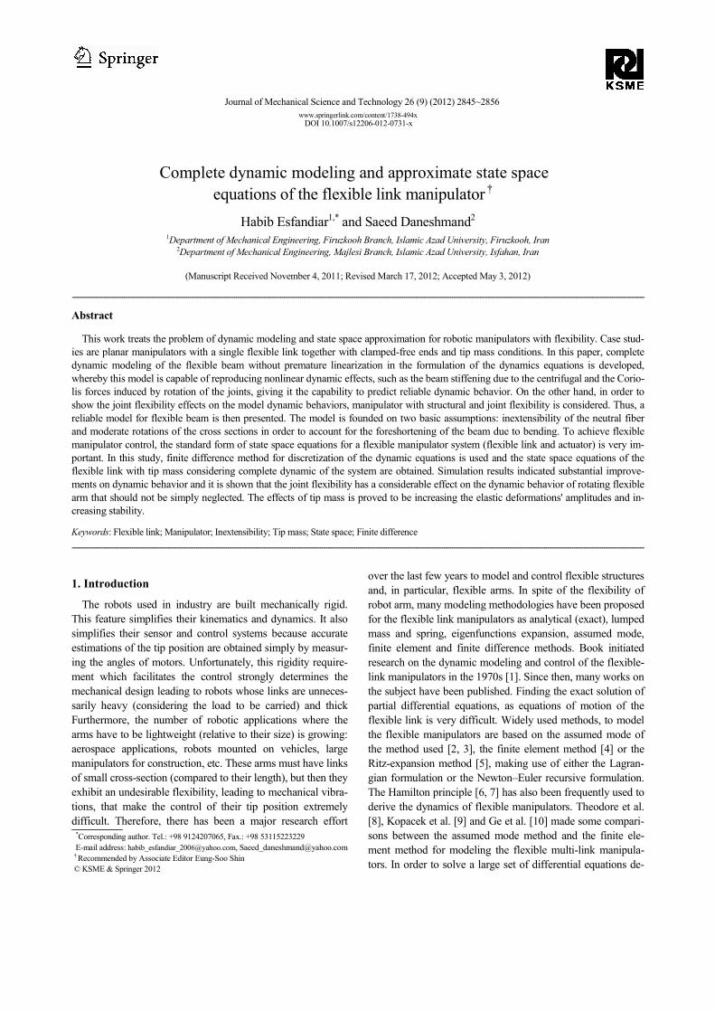
The coordinate systems used in developing the model are
shown in Fig. 1. Wherein, 0 0 0 0,O X Y Z is the inertial refer-
ence frame, 1 1 1 1,O X Y Z is a body coordinate system at-
tached to the motor shaft and 2 2 2 2,O X Y Z is another body
coordinate system attached to the hub such that its 2X axis is
H. Esfandiar and S. Daneshmand / Journal of Mechanical Science and Technology 26 (9) (2012) 2845~2856 2847
directed along the initial situation of the arm. The rotation of
frame 1 1 1 1,O X Y Z relative to frame 0 0 0 0,O X Y Z is de-
scribed by the angle ( )tθ and α denotes rotation of frame
2 2 2 2,O X Y Z relative to frame 1 1 1 1,O X Y Z . Consider a
flexible beam with length l fixed on the hub in the horizon-
tal plane. The joint is taken to have small torsional deforma-
tions. The hub is assumed to be rigid and the flexible link is
radially attached to the hub. The motion of the manipulator
system is described by the rigid body rotation ( )θ , the tor-
sional deformation angle ( )α which is measured relative to
the motor coordinate system and flexible displacement
( , )y x t of the beam. The rotatory inertia is also considered.
The beam is divided into n elements with the i th element
having two nodes i and 1i + and the transverse component
of the displacement vector of an infinitesimal link element is
described by ( , )y x t .
Having introduced the kinematics assumptions for the beam
deformation, the floating frame approach is now adopted in
order to develop the model equations. A coordinate system
2 2 2 2,O X Y Z is oriented such that the 2 2O X axis is coinci-
dent with the beam neutral axis, while axes 2 2O Y and
2 2O Z
are in the directions of the principal moments of the cross
section (Fig. 2).
3. Dynamic modeling of a flexible beam as the robot’s
arm
In this section we will consider flexible beam without joint
flexibility modeling in two different cases as follows:
(1) Flexible beam with both transverse and longitudinal vi-
brations and clamped (fixed)-free ends condition.
(2) Flexible beam with transverse vibration and tip mass.
3.1 Flexible beam with both transverse and longitudinal
vibrations and clamped-free ends conditions
In this section, we will consider dynamic modeling of a sin-
gle flexible link without joint flexibility with clamped-free
condition together with both transverse and longitudinal vibra-
tions. The position of an infinitesimal element of the link lo-
cated at a distance x from the frame origin in the 2 2O X di-
rection, relative to the 0 0 0 0,O X Y Z reference frame is given
by
( )( )
1
2
( , ) ( , ) cos ( , )sin
( , ) sin ( , )cos
d x t x u x t y x t e
x u x t y x t e
θ θ
θ θ
= + − +
+ +
(1)
where 1 2,e e ,3e are the unit vectors along the
0 0,X Y and
0Z axis, respectively.
According to this expression, the kinetic energy is involved
kinetic energy of the hub and kinetic energy of flexible link as:
( )
( ) ( ) ( ) ( )
1 12
2 2
1 2
2
1 22 2 2 2 22 22
r lKE I d d dx
H r
KE IH
r lx u x u y y x u y x u dx
r
θ ρ
θ
ρ θ θ θ θ
+= + ⋅∫
= +
++ + + + + + + − +∫
ɺ ɺɺ
ɺ
ɺ ɺ ɺ ɺɺ ɺ ɺ ɺ ɺ ɺ
(2)
where
⋅− denotes time derivative of ( )− and ( ) ( )− ⋅ −
denotes the dot product of vectors ( )− . The potential energy is
composed of the internal energy due to the elastic deformation
of the link due to bending and tension.
( ) ( )2 2
2
2
, ,1 1
2 2
r l r l
r r
y x t u x tPE EI dx EA dx
x x
+ +
∂ ∂= +∫ ∫
∂ ∂
(3)
where
( )2
,1
2
r l
r
u x tEA dx
x
+ ∂ ∂
∫
is the potential energy due to longitudinal vibration and the
potential energy due to gravity is not accounted for since only
the motion in the plane perpendicular to the gravitational field
is considered. For extracting equations of equations of motion,
the extended Hamilton principle is used as following:
( )2
1
0t
t
KE PE W dtδ δ δ− + =∫ (4)
Fig. 1. Rotary arm system.
Fig. 2. Mechanical model of a single flexible link.

2848 H. Esfandiar and S. Daneshmand / Journal of Mechanical Science and Technology 26 (9) (2012) 2845~2856
where
( )LW T tδ δθ= (5)
is the virtual work done by the torque applied at the hub,
( )T tL
. After a long process of computations, the following
dynamic equations can be obtained in terms of the two flexi-
ble displacements and rotation of the hub,
( ) ( )2 22 2 2
2 2 2 2
,y x td y dy EI x u
dt x x t dt
θ θρ ρ ρ
∂∂ ∂− + + + + +
∂ ∂ ∂
( , )2 0
u x t dfor r x r l
t dt
θρ
∂= ≤ ≤ +
∂ (6)
( )2 2
2
2
2
( , )
( , )2 0
d u u x tx u EA
dt x x t
d y x t dy
dt t dt
θρ ρ
θ θρ ρ
∂ ∂ ∂+ + − +
∂ ∂ ∂
∂+ =
∂
(7)
( ) ( ) ( ) ( )22
2
2 2
2 22
2 2
,2
( , ) ( , )2
r l
r
y x tu d dx u x u x u
t dt dt t dxy x t d d u x t
y y yt dt dt t
θ θρ ρ ρ
θ θρ ρ ρ
+
∂∂+ + + + + +
∂ ∂ +∫∂ ∂
+ −∂ ∂
( )2
2H L
dI T t
dt
θ= (8)
( )
( , ) 0
, 0
( , ) 0
y x t
yx r x t
x
u x t
=
∂= =∂
=
(9)
2
2
3
3
0
0
0
yEI
x
yx r l EIx
uEA
x
∂=
∂∂= + =∂∂
=∂
(10)
where Eqs. (6) and (7) are the system equations of motion, Eq.
(8) is the constraint equation expressing the total balance of
angular momentum of the system, Eq. (9) expresses the three
geometric boundary conditions at the clamped end of link and
Eq. (10) are the natural boundary conditions at the free end of
link. Moreover, initial conditions for ( ) ( ), ,t y x tθ and
( ),u x t require for solution set of the above equations such that
( ) ( )0 00 ,
d tin t t
dt
θθ θ θ= = = ɺ (11)
( ) ( )0 0
,, ,
dy x ty x t y y for r x r l
dt= = ≤ ≤ +ɺ
( ) ( )0 0
,, ,
du x tu x t u u
dt= = ɺ
where ( )0
− denotes value of ( )− , when 0t = . Thus, a
fourth order partial differential equation respected to ( , )y x t
and second order partial differential equation relative to
( , )u x t , six boundary conditions, six initial conditions and a
constraint equation expressing the overall balance of angular
momentum are obtained. In the set of mentioned equations,
terms are defined as Table 1.
3.2 Flexible beam with transverse vibration and tip mass
A payload is considered to be carried at the tip of the link
and this subject is motivated by modeling the flexible link
carrying a tip mass. In this section we consider a single flexi-
ble robot link without flexibility joint fixed in the hub along
with a lumped mass on the other end, therefore, the total ki-
netic energy of the flexible beam with a tip mass is the sum-
mation of translational and rotational kinetic energy of the
flexible beam, kinetic energy of the hub, translational and
rotational kinetic energy of the point mass, whose kinetic en-
ergy is as follows:
b b Tip Tip
t rot hub t rKE KE KE KE KE KE= + + + + (12)
( )( ) ( ) ( )( )2 2 2 2 21 1. , 2 ,
2 2
r l
Hr
KE I x y x t y x t x y x t dxθ ρ θ θ+
= + + + + +∫ɺ ɺ ɺɺ ɺ
( ) ( ) ( )( )2 21, 2 ,
2
r l
r
x y x t y x t dxφ θ θ+
′ ′+ + +∫ ɺ ɺɺ ɺ
( ) ( )( ) ( ) ( ) ( )2 2 2 21. , 2 ,
2t
M r l y r l t y r l t r l y r l tθ θ
+ + + + + + + + +ɺ ɺɺ ɺ
( ) ( )2 2 .1
, 2 ,2
J y r l t y r l tt θ θ
′ ′+ + + +ɺ ɺɺ ɺ (13)
To simplify
( )
( ) ( )( )
2 2 2
2 2
,
1.
2
r l r l
br r
t t
x y dx x dx I
M r l y r l t I
ρ ρ+ +
+ ≈ =∫ ∫
+ + + ≈ (14)
that tI is the inertia moment of the tip mass around the hub
and bI is the beam rotation inertia about the origin
0O , as if
it would be rigid. Using the same potential energy and virtual
work in the extended Hamilton principle, the following equa-
Table 1. Interpretation of the mathematical expression of Eqs. (6)-(8).
Description Transverse component Longitudinal
component
Centrifugal force
2d
ydt
θρ
( )2
dx u
dt
θρ
+
Force due to tan-
gential accelera-
tion
( )2
2
dx u
dt
θρ +
2
2
dy
dt
θρ
Coriolis force ( , )
2u x t d
t dt
θρ
∂
∂
( , )2
y x t d
t dt
θρ
∂
∂
Torque due to the
Coriolis force ( ) ( , )
2u x t d
x ut dt
θρ
∂+
∂
( , )2
y x t dy
t dt
θρ
∂
∂
Torque due to the
force due to tan-
gential accelera-
tion
( )2
2
2
dx u
dt
θρ +
22
2
dy
dt
θρ

H. Esfandiar and S. Daneshmand / Journal of Mechanical Science and Technology 26 (9) (2012) 2845~2856 2849
tions are derived,
( ) ( )
2 2 2 2
2 2 2 2
2
2
( , )0
y y dEI x
t x x dt
y x t dx x for r x r l
x t x t dt
θρ ρ
θφ φ
∂ ∂ ∂+ + −
∂ ∂ ∂
∂ ∂ ∂ ∂+ = ≤ ≤ +
∂ ∂ ∂ ∂
(15)
( )
( ) ( )
( ) ( ) ( )
2 2
2 2
2
2
2
2
( , )
,
r l
H b tr
r l
r
t L
d yI I I x dx
dt t
y x t dx x dx
t x t dt
d y r l tM r l T t
dt
θρ
θφ φ
+
+
∂+ + + +∫
∂
∂ ∂ ∂+ +∫
∂ ∂ ∂
++ =
(16)
( )
( , ) 0
, 0
y x t
for x r yx t
x
== ∂
=∂
(17)
( )
2 2 2
2 2 2
2 2 3
2 2 3
( , )0
0 .
d y x t yJ J EIt tdt t x x
for x r ly d y
M M r l EIt tt dt x
θ
θ
∂ ∂ ∂+ + =
∂ ∂ ∂= +
∂ ∂+ + − =
∂ ∂
(18)
As mentioned before, the initial conditions for ( )tθ and
( ),y x t are necessary for solving the set of above equations
illustrated in Eq. (11).
4. Finite dimensional equations (discretization)
The continuous models consist of partial differential equa-
tions difficult to deal with both analytically and computation-
ally. In order to obtain a set of ordinary differential equations,
a discretization of the equations developed previously must be
performed. The finite difference method is used to approxi-
mate partial differential equations described in the previous
sections with a set of ordinary differential equations. In this
method, the interval r x r l≤ ≤ + is divided into n uniform
segments with
lx h
n∆ = =
and , 0,1, ,ix r ih i n= + = … . Space derivatives are substituted
by finite differences such that the second and fourth spatial de-
rivatives are approximated with the second-order central differ-
ence approximation and the first spatial derivative is approxi-
mated with the first-order backward difference formula.
4
1 1 2 2
4
2
1 1
2 2
0 0 1
( ) 4 6 41,2, ,
4
( ) 2
( )
i i i i i i
n n n n
d y t y y y y yi n
dx h
d y t y y y
dx h
dy t y y
dx h
− + − +
− +
−
− + − + += =
− +=
−=
…
(19)
And third spatial derivative is approximated by
3
1 1 2
3 3
( ) 3 3n n n n nd y t y y y y
dx h− + +− + − +
= (20)
where the abbreviated notation ( )iy t and 0 ( )y t are used for
( , )iy x t and ( , )y r t , respectively. The point requiring atten-
tion is, that fourth order derivative in every point depends on
the information of five points, thus, meshing must have at
least four elements or five nodes. The elements consisting the
integral are discretized; the integral is replaced with summa-
tion ( )∑ and the beam is meshed from 0 to n intervals
such that first node in the mesh is on the hub and equals 0
and the final node is in x r l= + and equals n .
In this section, equations of the tip mass are considered and
terms relevant to rotational kinetic energy of the flexible beam
is neglected and the set of ordinary differential equations are
presented. Using finite difference, ordinary differential equa-
tions are,
1 1 2 2
4
4 6 40 1,2, ,
i i
i i i i i
y x
y y y y yEI for i n
h
ρ ρ θ
− + − +
+ +
− + − + += =
ɺɺɺɺ
…
(21)
( ) ( ) ( )2
20
ni
H b t i t n Li
yI I I x M r l y T t
tθ ρ
=
∂+ + + + + =∑
∂ɺɺ ɺɺ (22)
( )0
0 1
0
00
y
for x r i y y
h−
== = −
= (23)
( )
( )
1 1 1
2
1 1 2
20
3 30 .
3
n n n n nt t
n n n nt n t
or x r l i n
y y y y yJ J EI
h h
y y y yM y M r l EI
h
θ
θ
− + −
− + +
= + =
− − ++ + =
− + − ++ + − =
ɺɺ ɺɺɺɺ
ɺɺɺɺ
(24)
Since the boundary value of the solution is given for
0i = therefore, this approximation is applied for 1,2, ,i n= … ,
where:
For 1i =
1 2 31 1 4
6 40
y y yx y EI
hρ θ ρ
− ++ + =ɺɺ ɺɺ (25)
For 2,3, , 2i n= −…
1 1 2 2
4
4 6 40
i i
i i i i i
x y
y y y y yEI
h
ρ θ ρ
− + − +
+ +
− + − + +=
ɺɺ ɺɺ
(26)
For 1i n= −
2850 H. Esfandiar and S. Daneshmand / Journal of Mechanical Science and Technology 26 (9) (2012) 2845~2856
1 12 2 3
2 1 3
4
4 5 20
t t tn n n
n n n n
J J Jx y y
h h h
y y y yEI
h
θ ρ ρ− −
− − −
+ + + + − +
− + − +=
ɺɺ ɺɺ ɺɺ
(27)
For i n=
( )2 3
1 21 3 4
20 .
t t t tn n
t n n nn
M r l J M Jx y
h h h h
J y y yy EI
h h
θ ρ ρ
− −−
++ + + + +
− + ++ − + =
ɺɺ ɺɺ
ɺɺ
(28)
Discretization of the partial differential equation with re-
spect to the spatial variable replaces it by a set of ordinary
differential equations that can be written in matrix form as
1 1MZ KZ τ+ =ɺɺ (29)
where
0 0 0 0 0 0 0 0 0 0
0 6 4 1 0 0 0 0 0 0
0 4 6 4 1 0 0 0 0 0
0 1 4 6 4 1 0 0 0 0
4
0 0 0 0 0 0 4 6 4 1
0 0 0 0 0 0 1 4 5 2
0 0 0 0 0 0 0 1 2 1 1 1
EIK
h
n n
−
− −
− −=
− −
− −
− + × +
…
…
…
…
⋮ ⋮ ⋮ ⋮ ⋮ ⋮ ⋮ ⋮ ⋮ ⋮ ⋮
…
…
…
( )
( )
51 2 3 4 3 2 1
0 0 0 0 0 0 0 01
0 0 0 0 0 0 0 02
0 0 0 0 0 0 0 03
0 0 0 0 0 0 0 02
0 0 0 0 0 0 01 2 2 3
0 0 0 0 0 0 02 3 3
I I I x x x x x x x x x M r lnt tH n n nb
x
x
x
M
xn
J J Jt t txn h h h
M r l J J M Jt t t t txn h hh h h
ρ ρ ρ ρ ρ ρ ρ ρ ρ
ρ ρ
ρ ρ
ρ ρ
ρ ρ
ρ ρ
ρ ρ
+ + + +− − −
=
−
+ + −−
++ + − + +
…
…
…
…
⋮ ⋮ ⋮ ⋮ ⋮ ⋮ ⋮ ⋮ ⋮ ⋮ ⋮
…
…
…
( ) ( )1 1n n
+ × +
(30)
where 1Z is variables vector with 1n + elements defined
as:
1 1 2 ., , , , nZ y y yθ = … (31)
5. Simulation results
In order to illustrate the behavior of the previous models
under excitation pulse, the following section is presented.
5.1 Single flexible link under excitation pulse
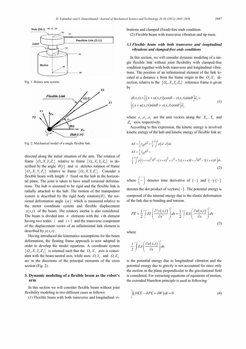
Time and amplitude of the pulse are 2 seconds and
0.55 .N m , respectively.
As Fig. 3 depicts, it is predicted that hub angle graph must
be composed of two parts such that, at time interval 1 sect = ,
the graph has its global maximum value and the angle value
doesn’t vary from 2 sect = to the end of the time interval,
where this situation consistent on physic of problem. Angular
velocity of the hub is also composed of two sections. Velocity
of rigid motion of the link and velocity relevant to elastic mo-
tion of the link around the situation. The produced graph must
explain the physic of the problem such that, until 1sect =
velocity increases, from 1 sect = to 2 sect = velocity de-
creases, and after 2 sect = , velocity is constant.
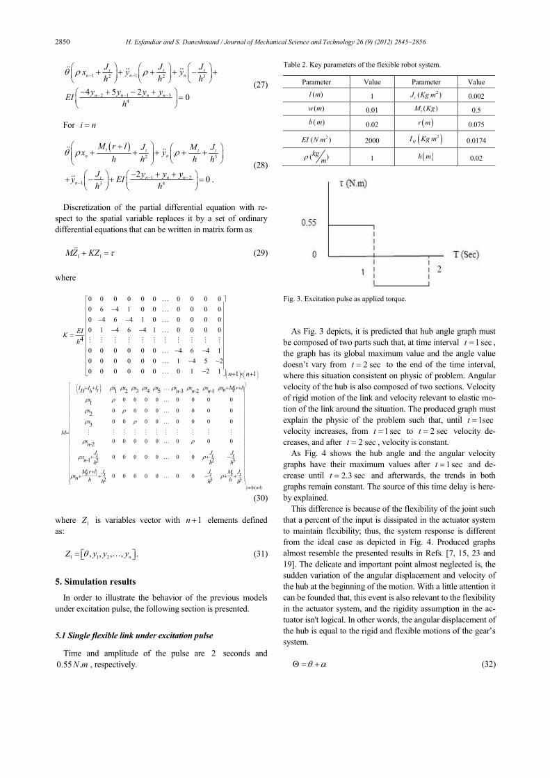
As Fig. 4 shows the hub angle and the angular velocity
graphs have their maximum values after 1 sect = and de-
crease until 2.3 sect = and afterwards, the trends in both
graphs remain constant. The source of this time delay is here-
by explained.
This difference is because of the flexibility of the joint such
that a percent of the input is dissipated in the actuator system
to maintain flexibility; thus, the system response is different
from the ideal case as depicted in Fig. 4. Produced graphs
almost resemble the presented results in Refs. [7, 15, 23 and
19]. The delicate and important point almost neglected is, the
sudden variation of the angular displacement and velocity of
the hub at the beginning of the motion. With a little attention it
can be founded that, this event is also relevant to the flexibility
in the actuator system, and the rigidity assumption in the ac-
tuator isn't logical. In other words, the angular displacement of
the hub is equal to the rigid and flexible motions of the gear’s
system.
θ αΘ = + (32)
Table 2. Key parameters of the flexible robot system.
Parameter Value Parameter Value
( )l m 1 2( )
tJ Kg m 0.002
( )w m 0.01 ( )tM Kg 0.5
( )b m 0.02 ( )r m 0.075
2( )EI N m 2000 ( )2
HI Kg m 0.0174
( )kg
mρ 1 ( )h m 0.02
Fig. 3. Excitation pulse as applied torque.
H. Esfandiar and S. Daneshmand / Journal of Mechanical Science and Technology 26 (9) (2012) 2845~2856 2851
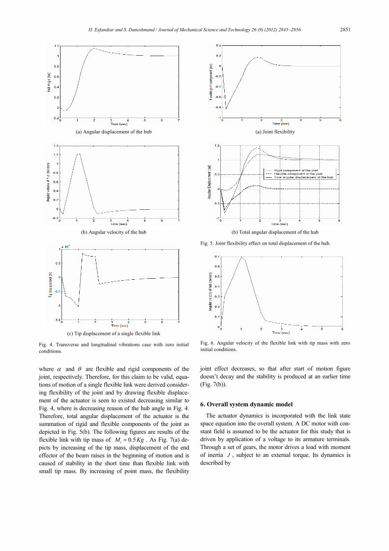
where α and θ are flexible and rigid components of the
joint, respectively. Therefore, for this claim to be valid, equa-
tions of motion of a single flexible link were derived consider-
ing flexibility of the joint and by drawing flexible displace-
ment of the actuator is seen to existed decreasing similar to
Fig. 4, where is decreasing reason of the hub angle in Fig. 4.
Therefore, total angular displacement of the actuator is the
summation of rigid and flexible components of the joint as
depicted in Fig. 5(b). The following figures are results of the
flexible link with tip mass of 0.5tM Kg= . As Fig. 7(a) de-
picts by increasing of the tip mass, displacement of the end
effector of the beam raises in the beginning of motion and is
caused of stability in the short time than flexible link with
small tip mass. By increasing of point mass, the flexibility
joint effect decreases, so that after start of motion figure
doesn’t decay and the stability is produced at an earlier time
(Fig. 7(b)).
6. Overall system dynamic model
The actuator dynamics is incorporated with the link state
space equation into the overall system. A DC motor with con-
stant field is assumed to be the actuator for this study that is
driven by application of a voltage to its armature terminals.
Through a set of gears, the motor drives a load with moment
of inertia J , subject to an external torque. Its dynamics is
described by
(a) Joint flexibility
(b) Total angular displacement of the hub
Fig. 5. Joint flexibility effect on total displacement of the hub.
Fig. 6. Angular velocity of the flexible link with tip mass with zero
initial conditions.
(a) Angular displacement of the hub
(b) Angular velocity of the hub
(c) Tip displacement of a single flexible link
Fig. 4. Transverse and longitudinal vibrations case with zero initial
conditions.

2852 H. Esfandiar and S. Daneshmand / Journal of Mechanical Science and Technology 26 (9) (2012) 2845~2856
m m m eJ T Tω = −ɺ (33)
where Te is the torque exerted on the motor shaft by the load,
transmitted through the gears. Thus,
e m m mT T J ω= − ɺ (34)
So the torque at the motor shaft is seen to be the torque gen-
erated by the motor, minus the torque required to accelerate
the rotor. The torque exerted by the motor on the load shaft,
transmitted through the gears, is eNT . Newton's second law
applied to the load is
.e L m L m m
J NT T NT T NJω ω= − = − −ɺ ɺ (35)
Since ,m Nω ω= this becomes
( )2
m m LJ N J NT Tω+ = −ɺ (36)
or
e m LJ NT Tω = −ɺ (37)
where 2
e mJ J N J= + is effective inertia seen at the load
shaft. We need the current i by Kirchhoff voltage law
m m
diL Ri V K
dtω+ = − (38)
where mK ω is the back emf and equations in matrix form is:
.
0 1 0 0 0
10 0 0
100
m
e L
m
Vd NK
dt J J Tei i
NK R
LL L
θ θω ω
= + −
− −
(39)
By selection of θ and ω as the outputs, the output equa-
tion is:
.1 0 0
0 1 0i
θθ
ωω
= (40)
The simulation conditions are as follows: with zero
conditions for the state variables and ( ) 0,LT t =
( ) 3 0 2V t volt t= ≤ ≤ and ( ) 3 2 4V t volt t= − < ≤ , and
0.05 / , 1.2 , 0.05mK Nm A R L H= = Ω = 4 2 28 10 . , 0.02 .
mJ kg m J kg m−= × = and 12N = . Time
response of DC motor has been shown in Fig. 8.
7. Approximate state space equations
For the purpose of the flexible manipulator control (future
work), we need a standard form of the state space equations
for a flexible manipulator system (flexible link and actuator).
The finite difference method is used to approximate partial
differential equations with a set of ordinary differential equa-
tions as,
1 1.MZ KZ τ+ =ɺɺ (41)
And from latter section, we derived the state space equation of
actuator. In this section, we want to derive state space equa-
tions of total system. Therefore, for writing the closed form of
Fig. 8. Time response for the DC motor.
(a) Tip displacement
(b) Angular displacement of the hub
Fig. 7. The effect of increasing tip mass on tip displacement and angu-
lar velocity of the hub.
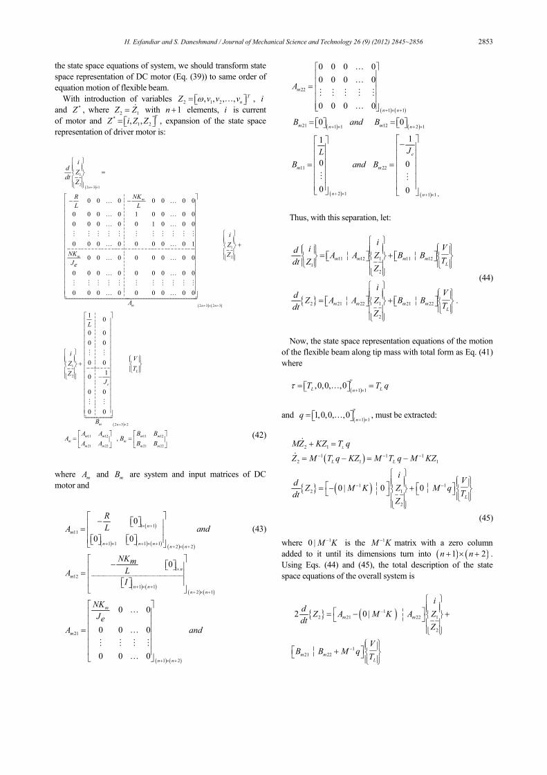
H. Esfandiar and S. Daneshmand / Journal of Mechanical Science and Technology 26 (9) (2012) 2845~2856 2853
the state space equations of system, we should transform state
space representation of DC motor (Eq. (39)) to same order of
equation motion of flexible beam.
With introduction of variables 2 1 2, , , , T
nZ v v vω = … , i
and *Z , where 2 1
Z Z= ɺ with 1n + elements, i is current
of motor and *
1 2, ,T
Z i Z Z = , expansion of the state space
representation of driver motor is:
( )
1
22 3 1n
id
Zdt
Z+ ×
=
2
0 0 0 0 0 0 0
0 0 0 0 1 0 0 0 0
0 0 0 0 0 1 0 0 0
0 0 0 0 0 0 0 0 1
0 0 0 0 0 0 0 0
0 0 0 0 0 0 0 0 0
0 0 0 0 0 0 0 0 0
m
m
m n
R NK
L L
NK
Je
A
− −
… …
… …
… …
⋮ ⋮ ⋮ ⋮ ⋮ ⋮ ⋮ ⋮ ⋮ ⋮ ⋮
… …
… …
… …
⋮ ⋮ ⋮ ⋮ ⋮ ⋮ ⋮ ⋮ ⋮ ⋮ ⋮
… …
( ) ( )
1
2
3 2 3n
i
Z
Z
+ × +
+
( )
1
2
2 3 2
10
0 0
0 0
0 0
10
0 0
0 0
L
e
m n
L
iV
ZT
Z
J
B + ×
+
−
⋮ ⋮
⋮ ⋮
11 12 11 12
21 22 21 22
,m m m m
m m
m m m m
A A B BA B
A A B B
= = (42)
where mA and
mB are system and input matrices of DC
motor and
( )
( ) ( ) ( ) ( ) ( )
1 1
11
1 1 1 12 2
0
0 0
n
m
n n nn n
R
LA and× +
+ × + × ++ × +
−= (43)
( ) ( )( ) ( )
1
12
1 12 1
0n
m
n nn n
NKmLAI
×
+ × ++ × +
−=
( ) ( )
21
1 2
0 0
0 0 0
0 0 0
m
m
n n
NK
Je
A and
+ × +
=
…
…
⋮ ⋮ ⋮ ⋮
…
( ) ( )
22
1 1
0 0 0 0
0 0 0 0
0 0 0 0
m
n n
A
+ × +
=
…
…
⋮ ⋮ ⋮ ⋮ ⋮
…
( ) ( )21 121 1 2 10 0
m mn nB and B
+ × + × = =
( ) ( )
11 22
2 1 1 1 .
11
0 0
0 0
e
m m
n n
JL
B and B
+ × + ×
−
= =⋮ ⋮
Thus, with this separation, let:
11 12 1 11 12
1
2
2 21 22 1 21 22
2
.
m m m mL
m m m m
L
iVid
A A Z B BTdt Z
Z
iVd
Z A A Z B BTdt
Z
= +
= +
(44)
Now, the state space representation equations of the motion
of the flexible beam along tip mass with total form as Eq. (41)
where
( )1 1,0,0, ,0
T
L LnT T qτ
+ × = =…
and ( )1 1
1,0,0, ,0T
nq
+ × = … , must be extracted:
( )
( )
2 1
1 1 1
2 1 1
1 1
2 1
2
0 | 0 0
L
L L
L
MZ KZ T q
Z M T q KZ M T q M KZ
iVd
Z M K Z M qTdt
Z
− − −
− −
+ =
= − = −
= − +
ɺ
ɺ
(45)
where 10 | M K− is the 1M K− matrix with a zero column
added to it until its dimensions turn into ( ) ( )1 2n n+ × + .
Using Eqs. (44) and (45), the total description of the state
space equations of the overall system is
( )1
2 21 22 1
2
1
21 22
2 0 |m m
m m
L
id
Z A M K A Zdt
Z
VB B M q
T
−
−
= − +
+

2854 H. Esfandiar and S. Daneshmand / Journal of Mechanical Science and Technology 26 (9) (2012) 2845~2856
( )1
21 22 1
22
1
21 22
0 |1
2
m m
m mL
i
A M K A Zd ZZdt
VB B M q
T
−
−
− +
=
+
(46)
and the closed form is
( )( ) ( )
11 12
11 1
21 22
2 2
1 10 |
2 2
m m
m m
i iA Ad
Z ZA M K Adt
Z Z
A
−
= +−
( ) ( )11 12
1
21 22
1 1
2 2
m m
Lm m
B BV
TB B M q
B
−
+
.X AX BU= +ɺ (47)
Selecting angular position of the flexible beam and tip de-
flection of the beam as output variables, as the output equation,
let
( ),Y
y r l t
θ
=+
( )
1
2
2 2 3
0 1 0 0 0 0 0 0 0
0 0 0 0 1 0 0 0 0
n
i
Y Z
ZC × +
= +
… …
… …
( )2 2
0 0
0 0 L
V
T
D
Y CX DU
×
= +
(48)
where only ( ) ( )1,2 2, 2 1Y Y n= + = .
7.1 General control problem
In this section, we consider a general control problem. Fig.
9 shows the general control configuration, where ( )G s is the
generalized plant model and it will include the interconnection
structure between the plant and the controller. ( )G s is the
generalized controller.
For control purposes, Eqs. (47) and (48) can be rewritten to
the augmented state space model as,
1 2
1 11 12
2 21 22
( )
A B B
G s C D D
C D D
= (49)
where
( )( ) ( )( ) ( )
11 12
1
21 22
2 3 2 3
1 10 |
2 2
m m
m m
n n
A A
AA M K A−
+ × +
=−
(50)
( )( )
( )( )
11 12
1 2 1
21 22
2 3 1 2 3 1
,1 1
2 2
m m
m m
n n
B B
B BB B M q−
+ × + ×
= =+
( )1 1 2 30 1 0 0 0 0 0 0 0
nC × + = … …
( )2 1 2 30 0 0 0 1 0 0 0 0
nC × + = … …
11 12 21 22 0 .D D D D= = = =
Therefore, the augmented state space model has been ob-
tained and it is ready for implementing control methods.
Clearly, state equation (Eq. (47)) has incorporated manipulator
motion (hub rotation and link deflection), actuator dynamics,
as well as sensor specification. The system matrix A is a
function of link construction (mass and stiffness distributions)
and actuator design (motor parameters), while the output ma-
trix C is a function of beam position and tip deflection.
8. Conclusions
This paper treated the problem of dynamic modeling and
state space representation for robotic manipulators with flexi-
bility. A systematic top-down approach to the modeling of
flexible robotic links was undertaken. In this paper, complete
dynamic modeling of a flexible beam without the premature
linearization in the formulation of the dynamics’ equations
was developed, whereby the model is capable of reproducing
nonlinear dynamic effects, such as the beam stiffening due to
the centrifugal and the Coriolis forces induced by rotation of
the joints. On the other hand, joint flexibility effects on the
model dynamic behaviors were shown. The model is founded
on two basic assumptions: inextensibility of the neutral fiber
and moderate rotations of the cross sections in order to ac-
count for the foreshortening of the beam due to bending. It is
essential to notice that the sudden variation of the angular
displacement and velocity of the hub in the beginning of the
motion, is an event relevant to the flexibility in the actuator
system. In other words, angular displacement of the hub is
equal to rigid and flexible motions of the actuator system. For
Fig. 9. Most general control system.
H. Esfandiar and S. Daneshmand / Journal of Mechanical Science and Technology 26 (9) (2012) 2845~2856 2855
the flexible arm with tip mass, when the value of the lumped
mass increases thus the end- effector displacement of the arm
also increases in the beginning of motion and is caused of the
stability in the short time than flexible link with small tip mass
and the flexibility joint effect decreases, so that after start of
the motion, angular displacement and velocity don’t decay
and the stability is produced at an earlier time. Simulation
results and resulting model have indicated considerable im-
provements on dynamic behavior and have shown that the
joint flexibility has a substantial effect on the dynamic behav-
ior of rotating flexible arm that should not be simply neglected.
To achieve enhanced control, the state space equations were
obtained and work is ready for implementing control methods.
Nomenclature------------------------------------------------------------------------
l : Length of link
w : Width of link
E : Height of link
I : Cross section moment of inertia
A : Cross section of link
E : Young Modulus
EI : Stiffness of the link
ρ : Specific mass per unit of length of beam
x : The position of an infinitesimal element of the link
from the absolute frame origin
HI : Moment of inertia of the hub
r : Radius of the hub
( )tθ : Reference angular motion
α : Torsional deformation angle
LT : Torque applied at the hub
( , )y x t : Transverse vibration component of an infinitesimal
element of beam
( , )u x t : Longitudinal vibration component of an infinitesimal
element of beam
ψ : Rotation of the flexible beam
tM : Tip mass
tJ : Moment of inertia of tip mass
( )xφ : Moment of inertia per unit length of beam b
tKE : Translational kinetic energy of flexible link
b
rotKE : Rotational kinetic energy of flexible link
hubKE : Rotational kinetic energy of rigid hub Tip
tKE : Translational kinetic energy of tip mass
Tip
rKE : Rotational kinetic energy of tip mass
KEδ : Virtual differential of kinetic energy
PEδ : Virtual differential of potential energy
Wδ : Virtual work
M : System mass matrix
K : System stiffness matrix
τ : Force column vector
eJ : Effective inertia of load shaft of a DC motor
N : Gear ratio of motor
V : Armature voltage
i : Armature current
R : Resistance of armature circuit
L : Inductance of armature circuit
mT : Produced torque by a DC motor
J : Moment of inertia of load
n : Number of elements
h : Step size
References
[1] W. J. Book, Modeling design and control of flexible manipu-
lator arms, Ph.D. Dissertation, MIT University, USA, April
(1974).
[2] D. L. Wang, Y. F. Lu, Y. Liu and X. G. Li, Dynamic model
and tip trajectory tracking control for a two-link flexible ro-
botic manipulator, Proceedings of the IEEE Conference on
System, Man and Cybernetics, Beijing, China (1996) 1020-
1024.
[3] GB. Yang and M. Donath, Dynamic model of a one-link
manipulator with both structural and joint flexibility, Pro-
ceedings of the IEEE Conference on Robotics and Automa-
tion, Philadelphia (1988) 476-481.
[4] S. S. Ge, T. H. Lee and G. Zhu, Nonlinear feedback control-
ler for a single-link flexible manipulator based on finite ele-
ment model, Journal Robotic Systems, 14 (3) (1997) 165-
178.
[5] S. Nicosia, P. Valigi and L. Zaccarian, Dynamic modeling of
a two link flexible robot and experimental validation, Pro-
ceedings of the IEEE Conference on Robotics and Automa-
tion, Minnesota, USA (1996) 1953-1957.
[6] K. L. Low and M. Vidyasagar, A Lagrangian formulation of
the dynamic model for flexible manipulator systems, Journal
of Dynamic Systems Measurement and Control, 110 (2)
(1988) 175-181.
[7] J. Martins, M. A. Botto and J. S. Costa, Modeling of flexible
beams for robotic manipulators, Multi body System Dynam-
ics, 7 (1) (2002) 79-100.
[8] R. J. Theodore and A. Ghosal, Comparison of the assumed
modes method and finite element models for flexible multi
link manipulators, Journal of Robotic Research, 14 (2)
(1995) 91-111.
[9] P. Kopacek, K. Desoyer and P. Lugner, Modeling of flexible
robots-an introduction, in Proc, IFAC Robot Contr, 10 (1)
(1989) 21-27.
[10] S. S. Ge, T. H. Lee and G. Zhu, Comparison studies be-
tween assumed modes method and finite element method in
modeling a single-link flexible manipulator, Proceedings of
the IEEE International Conference on Intelligent Control
and Instrumentation, Singapore (1995) 376-381.
[11] S. K. Tso, T. W. Yang, W. L. Xuc and Z. Q. Sun, Vibration
control for a flexible-link robot arm with detection feedback,
Journal of Non-Linear Mechanics, 38 (1) (2003) 51-62.
[12] P. W. Likins, Mathematical modeling of spinning elastic
bodies, AIAA Journal, 38 (1) (1973) 51-62.
[13] P. Zhou, F. Y. Wang, W. Chen and P. Lever, Optimal con-
struction and control of flexible manipulators: a case study
based on LQR output feedback, journal of Mechatronics, 11

2856 H. Esfandiar and S. Daneshmand / Journal of Mechanical Science and Technology 26 (9) (2012) 2845~2856
(1) (2001) 59-77.
[14] B. Chapnik, G. Heppler and J. Aplevich, Modeling impact
on a one link flexible robot arm, IEEE Transactions on Ro-
botics and Automation, 7 (4) (1991) 479-488.
[15] R. Somaraju, Modelling and control of a single flexible
beam, Ph.D. Dissertation, University of Auckland, New
Zealand, September 14 (2005).
[16] T. Yokohama, Free vibration characteristics of rotating
Timeshenko beams, Journal of Mechanical Science, 30 (10)
(1988) 743-755.
[17] J. R. Velthius, T. J. AdeVries and J. van Amerongen,
Learning feed forward a flexible beam, Proceedings of the
1996 IEEE International, Symposium on Intelligent Control,
Dearborn, September (1996) 103-108.
[18] K. H. Low, Vibration analysis of a top-loaded beam at-
tached to a rotating joint, Computers and Structures, 52 (5)
(1994) 955-968.
[19] B. O. Al-Bedoor and A. A. Almusallam, Dynamics of
flexible-link and flexible-joint manipulator carrying a pay-
load with rotary inertia, Mechanism and Machine Theory, 35
(1) (2000) 785-820.
[20] R. Featherstone and D. Orin, Robot dynamics-equations
and algorithms, IEEE International Conference Robotics &
Automation, San Francisco, USA (2000) 826-834.
[21] J. A. Somolinos, V. Feliu and L. Sanchez, Design, dynamic
modeling and experimental validation of a new three-degree-
of-freedom flexible arm, Mechatronics, 5212 (1) (2002)
919-948.
[22] S. Moberg, On modeling and control of flexible manipula-
tors, PhD Thesis, No. 1336, Linköping University, Sweden
(2007).
[23] M. Gu and J. C. Piedb, A flexible arm as manipulator posi-
tion and force detection unit, Control Engineering Practice,
11 (12) (2003) 1433-1448.
H. Esfandiyar is a PhD student of Me-
chanical Engineering at Department of
Mechanical and Aerospace Engineering,
Science and Research Branch, IAU,
Tehran, Iran. His current research inter-
ests include robotic, composite and vi-
bration.
S. Daneshmand is a PhD student of
Mechanical Engineering at Department
of Mechanical and Aerospace Engineer-
ing, Science and Research Branch, IAU,
Tehran, Iran. His current research inter-
ests include robotic, rapid prototyping
and rapid tooling.