competitive efiects of vertical integration with downstream ... · competitive efiects of...
TRANSCRIPT

Competitive Effects of Vertical Integration with Downstream
Oligopsony and Oligopoly
Simon Loertscher and Markus Reisinger∗
March 26, 2008
Abstract
This paper analyzes the competitive effects of backward vertical integration by a par-tially vertically integrated firm that competes a la Cournot with non-integrated firms bothon the upstream and on the downstream market. We find under general conditions thatvertical integration is only anticompetitive if the ex ante degree of integration is high andthe number of competitors is large. That is, for most cases vertical integration has a pro-competitive effect and leads to a price decrease of the final output. This result contrastswith previous findings of slightly different market structures, e.g. a dominant firm model.Therefore, the present model’s implications for the regulation of vertical mergers differ fromthe previous literature by suggesting a more permissive approach.
Keywords: Vertical Integration, Downstream Oligopsony, Downstream Oligopoly, Capacity
Choice
JEL-Classification: D41.
∗Emails: [email protected] and [email protected] Financial support through aResearch Grant by the Faculty of Economics and Commerce at the University of Melbourne is gratefully ac-knowledged.
1
1 Introduction
Over the last two decades substantial progress has been made on identifying procompetitive
and anticompetitive effects of vertical mergers. After the Chicago School critique on the relative
aggressive enforcement policy on vertical mergers in the 1960’s, several theories have emerged
that base the potential competitive effects of vertical integration on more solid ground. Yet,
there is no general consensus under which conditions a merger is likely to benefit or harm
consumers and decrease (or increase) final good prices. The elimination of double marginal-
ization has been identified as a major efficiency gain from vertical integration. On the other
hand, the merging parties may be inclined to raise the input prices to their rivals and thereby
induce market foreclosure. As a consequence of this trade-off, vertical mergers are often judged
by antitrust authorities and courts on a case-by-case basis. General conclusions under which
conditions either effect dominates are not easily gained.1
Moreover, many models that identify different aspects of vertical mergers are not readily
applicable for policy implications because they are unsatisfactory in two important aspects.
First, merging parties often claim to merge because of efficiency gains in production that lead
to cost reductions. This means that they not only avoid double marginalization but are also
able to produce the output good in a different and more efficient way than without integration.
This effect is not captured in several well-known models (e.g. Ordover, Saloner, and Salop,
1990; Hart and Tirole, 1990; Choi and Yi, 2000). Second, firms that have oligopolistic market
power in the downstream market often also exert oligopsonistic market power when buying the
intermediate goods. Yet, many important models do not take this into account explicitly (e.g.
Salinger, 1988; Chen, 2001).
A notable exception is Riordan (1998) who considers a model with a dominant firm and a
competitive fringe in the downstream market. To produce the final good, firms need a fixed
input, termed capacity, that is competitively offered on an upward sloping supply curve. The
dominant firm exerts market power both downstream and on the input market. The more
capacity a firms owns the lower are its production costs of the final good. Therefore, the model
is not open to the two criticisms above. If the dominant firm integrates backwards, it acquires
more capacity and so produces more output. On the other hand, since demand of capacity
increases, the price of capacity increases as well and so fringe firms are foreclosed. Riordan
(1998) shows that the second effect always dominates and vertical integration is anticompetitive1For recent surveys on the effects of vertical mergers, see Riordan (2008) and Rey and Tirole (2007).
2
in that it leads to a decrease in output and to an increase in the final good price. A drawback of
the model by Riordan (1998) is that it can only be applied under the rather rare circumstances
where the final good market is comprised of a dominant firm facing a competitive fringe.
The present paper provides an analysis of an oligopolistic downstream market in which
the structure of the model is close the one of Riordan (1998). We show that the conclusions
about the competitive effects of vertical integration differ substantially from the dominant firm
model. In an oligopolistic market structure vertical integration is only anticompetitive if the ex
ante degree of integration is high and the number of downstream competitors is large. Thus,
for many circumstances vertical integration is procompetitive. As a consequence, our policy
implications differ substantially from those in the dominant firm model. They are also clear
cut and can be easily checked in most cases of vertical integration. Especially, in industries
that exhibit almost no integration in the first place vertical integration is likely to be beneficial
to consumers. Competition authorities need only be wary if an already largely integrated firm
plans to integrate further.
The intuition behind our result is the following. If a firm integrates backwards it increases
its capacity and produces a higher amount of output due its lower production costs. Thus, there
is a positive direct effect of integration. As a consequence of that, the input price increases
and so its rivals lower their capacity and produce less. We show that in an oligopolistic market
the direct effect is larger than the indirect effects and, as a result, more capacity is used. The
countervailing effect is that the firm with a larger capacity uses this capacity less efficiently
than its rivals. The reason is that it has the ability to produce more and so can gain more
from a higher price. Thus, it is less inclined to expand its quantity and utilizes its capacity to
a smaller extent than smaller rival firms. This second effect is the driving force in the model
of Riordan (1998) and is the decisive effect why vertical integration is anticompetitive. This
contrasts with an oligopolistic market structure, where this effect is dominated by the direct
capacity expansion effect as long as the ex ante degree of vertical integration is not excessively
high. This can even go so far that monopolizing the downstream market is welfare enhancing
as long as the number of possible producers is not too large. For example, in a model with
linear demand and quadratic costs we show that a firm that is vertically integrated to such an
extent that all rivals are foreclosed and that thereby monopolizes the market produces a larger
quantity than an oligopoly that consists of no more than three firms downstream.
As mentioned, most of the literature on vertical integration is mainly concerned with the
3

trade-off between avoidance of double marginalization and foreclosure. Hart and Tirole (1990)
or Ordover, Saloner, and Salop (1990), where no efficiency gains from vertical integration are
present, are only concerned with the foreclosure motives. In Salinger (1988), Choi and Yi (2000)
and Chen (2001) both effects are present but although the downstream market is comprised of
an oligopoly or a duopoly, downstream firms have no market power in the intermediate good
market. A recent model that incorporates both effects and additionally allows downstream firms
to exert market power in the intermediate good market is Hendricks and McAfee (2007). In their
model upstream firms can overstate their cost function while downstream firms can understate
their revenue function in the output market. The intermediate good market clears by bringing
the reports of both sides together, and the solution technique is similar to the supply function
approach of Klemperer and Meyer (1989). Hendricks and McAfee’s model is more general than
ours with respect to the upstream market because they allow for a general number of firms
while we impose this market to be perfectly competitive. On the other hand, when analyzing
vertical mergers they keep the downstream price fixed and suppose that the market structure
consists of no vertical integration at the outset. They show that under these assumptions
output always increases with vertical mergers. In contrast, in our model the downstream price
is flexible and we show that a crucial variable to determine the competitive effects of vertical
integration is the degree to which the industry is already integrated: Vertical integration is
procompetitive as in Hendricks and McAfee (2007) if there is no ex ante integration but it may
become anticompetitive if the existing degree of vertical integration is already high.
Our result that vertical integration is procompetitive if the industry is not yet characterized
by a high degree of vertical integration seems also consistent with recent empirical evidence and
with court decisions. For example, Hortacsu and Syverson (2007) study vertical integration
in the cement and ready-mixed concrete industries during 1963 to 1997. During this time the
extent of vertical integration increased heavily in both industries. Yet, in each market there
is still a large number of firms present and no firm had a dominant position. Hortacsu and
Syverson (2007) find that in both industries quantities increased and prices decreased steadily
during this time which is consistent with our findings.
A different example in which vertical integration is considered to be procompetitive is given
by a recent decision of the Competition Commission (CC) in the UK. In October 2006 the CC
cleared a merger between English Welsh & Scottish Railway Holdings (EWS) and Marcroft
Engeneering. EWS is the largest operator of rail freight haulage services in Great Britain,
4
while Marcroft is the largest supplier of rail freight wagon maintenance. Both companies have
a market share in their respective markets of more than 50 percent and so the potential for
foreclosure is relatively high. Yet, the CC cleared the merger with the lowest remedy that was
proposed by the Office of Fair Trading, namely the divestiture of only some parts of Marcroft’s
outstation business. Previous models would conclude that such a merger is very likely to be
welfare reducing because it almost monopolizes the industry. In light of the the predictions of
our model, such a merger would be welfare reducing only if there is large number of downstream
competitors and the market would shift from being relatively competitive to being dominated
by one firm. But in the haulage market there are only two competitors present (Freightliner
and Direct Rail Services). As a consequence, the CC decision is consistent with the predictions
of our model that, although the market is dominated by the integrated firm after the merger,
the efficiency gains may well dominate foreclosure motives in this case.
The remainder of the paper is organized as follows. Section 2 lays out the model. Section
3 presents the solution to the model and gives conditions under which vertical integration
is procompetitive or anticompetitive. In Section 4 we derive some explicit solutions for the
linear-quadratic case. Section 5 concludes. Longer proofs and derivations are in the Appendix.
2 Model
The following model is adapted from Riordan (1998) with some minor differences with respect
to timing. We also assume that the vertically integrated firm has no inherent cost advantage
in production (i.e. γ = 0 in his notation). The main difference is, of course, that we assume
a downstream oligopoly in contrast to his assumption of a dominant firm and a competitive
fringe.
We study a dynamic game with complete information. There are two types of firms, one
vertically integrated firm, which we index by I and N ≥ 1 non-integrated firms. A typical
non-integrated firm is indexed by j.2
All firms produce a homogenous good sold a la Cournot on the downstream market, where
the inverse demand function is P (Q) with P ′ < 0, where P is the market clearing price for
aggregate quantity Q ≡ qI +∑N
j=1 qj . To ensure existence and uniqueness of equilibrium in
the quantity stage, we also impose the sufficient condition P ′′ ≤ 0.2We use lower case index letters mainly, though not exclusively to denote non-integrated firms. The index j
is exclusively used for non-integrated firms.
5
Total costs of producing qi units are
ci(qi, ki) = kiC
(qi
ki
)(1)
for all firms j ∈ I, 1, ..., N , where ki is firm i’s production cost reducing capacity chosen in
stage 1 and ci(.) exhibits constant returns to scale in qi and ki and increasing marginal costs
in qi, with i = I, 1, .., N . That is, doubling ki and qi will double ci while C ′ ≥ 0 and C ′′ > 0.3
Firm I’s initial capacity endowment, i.e. its ex ante (or exogenous) degree of vertical
integration, is k > 0. The competitive inverse supply function of capacity is R(K) with R′ > 0
and K ≡ kI +∑N
j=1 kj .
The timing is as follows.
• Stage 1: The Capacity Stage. The ex ante degree of vertical integration k is ex-
ogenously given and common knowledge. All firms i simultaneously choose their level of
capacity ki. Firm I buys kI −k at the market price R(kI +∑N
j=1 kj). Observe that I has
the opportunity to sell undesired capacity, which occurs if kI < k.
• Stage 2: The Quantity Stage. Having observed all the capacity levels k = (kI , k1, .., kN )
all firms choose simultaneously their quantities qI , q1, .., qN . A Cournot-Walras auctioneer
announces the market clearing price P (Q) and the game ends, where Q ≡ ∑Nj=1 qj + qI .
We focus on subgame perfect equilibria that are symmetric, i.e. on equilibria where the
non-integrated firms play the same strategies. The quantity subgame following the choice of
capacity k is called the k-subgame.
3 General Equilibrium Properties
The following results obtain under general assumptions.
3.1 The Quantity Stage (Stage 2)
We begin with a simple result that has several important implications.
Lemma 1 Every k-subgame has a unique equilibrium.
Proof : The first order condition for a profit maximum in the k-subgame for firm i is4
P (Q) + P ′(Q)qi = C ′i
(qi
ki
). (2)
3This type of cost function was introduced by Perry (1978); see also Hendricks and McAfee (2007).4To save on notation, here and in the following we abbreviate C
(qiki
)by Ci.
6

Note that at this stage there is no intrinsic difference between an integrated and a non-integrated
firm. It is also readily checked that the second order condition is satisfied. Moreover, if the
quantities of all firms other than i are zero, then i optimally sets a positive quantity, while
its optimal quantity is zero if the aggregate quantity of all other firms is sufficiently large.
Finally, the slope of the reaction function of firm i is negative but larger than −1. Therefore,
an equilibrium (in pure strategies) is guaranteed to exist and to be unique. ¥ We denote
by Q(k) the aggregate equilibrium quantity given any vector of capacities k and by qi(k) the
corresponding equilibrium quantity of firm i with i = I, 1, .., N .
Corollary 1
qh(k) > ql(k) ⇔ kh > kl. (3)
Proof : Suppose to the contrary that kh > kl but qh ≤ ql. But then the right hand side of (2)
is strictly smaller for h than for l because Ci is convex in qi and decreasing in ki while the left
hand side is is (weakly) larger for h than for l, which is a contradiction. Conversely, if qh > ql,
the left hand side of (2) is smaller than the right hand side. Since Ci is convex, kh must be
bigger than kl. ¥
Corollary 2
ki = 0 ⇒ qi(k) = 0 and limki→0
qi(k)ki
> 0.
Proof : Because Ci is strictly convex, C ′i is invertible and equation (2) can be written as
qi
ki= C
′−1i
(P (Q) + P ′(Q)qi
)(4)
or equivalently as
qi = kiC′−1i
(P (Q) + P ′(Q)qi
). (5)
Now ki = 0 ⇒ qi = 0 follows directly from (5). Observe that the inverse C′−1i (.) is strictly
increasing and zero if and only if its argument is zero. Since all firms that produce a positive
quantity face positive marginal costs, P (Q) > 0 holds in equilibrium. Moreover, since as ki
approaches zero qi approaches zero,
limki→0
qi
ki= lim
qi→0C′−1i
(P (Q) + P ′(Q)qi
)= C
′−1i (P (Q)) > 0. (6)
¥
Corollary 3 qh(k)kh
decreases in kh.
7

Proof : If kh > kl then we know from the last Corollary that qh > ql. But this implies that
the left hand side of (2) is smaller for h than for l. As a consequence, the right hand side must
be smaller as well. Since Ci is convex it follows that qhkh
< qlkl
. The only if part can be proved
by following the steps in the opposite direction. ¥
Corollary 4qi(k)ki
>dqi(k)dki
∀i ∈ {I, 1, ..., N} (7)
Proof : Due to Corollary 3, d(qi/ki)dki
< 0 holds. That is, d(qi/ki)dki
= (dqi/dki)ki−qi
k2i
< 0, which in
turn implies dqidki
− qiki
< 0. ¥
The following Lemma states that all own effects of capacity on quantity are positive and
all cross effects are negative, which is very intuitive.
Lemma 2dqi(k)dki
> 0 for all i anddqm(k)
dki< 0 for i 6= m. (8)
The proof of the second part is rather long and therefore relegated to the Appendix. The first
part is already implied by Corollary 1.
3.2 The Capacity Stage (Stage 1)
We now move on to the first stage of the game, the capacity choice game. We now assume
that P ′′ and C ′′′ are small compared to P ′, C ′′, R′ and R′′, so that we can safely ignore them.5
Throughout the paper, we focus on stable equilibria.6 Next we establish the very intuitive
result that the integrated firm is the largest firm (where size is measured in units of capacity)
and that its capacity increases in k.
Proposition 1dkI
dk> 0 and
dkj
dk< 0 ∀j ∈ {1, ..., N}.
The proof is in the appendix. Proposition 1 has the following corollary:
Corollary 5 k∗I (k) > k∗j (k) ⇔ k > 0.
Corollary 3, Lemma 2 and Proposition 1 immediately imply the following result:5Notice that the model is still slightly more general than a linear quadratic model because we still allow that
P ′ and C′′ differ if the arguments of these functions differ. We only require the difference to be small.6A model that has a unique stable equilibrium is the model with linear demand and quadratic cost functions
analyzed in Section 4 below.
8

Proposition 2 qIkI
<qj
kjand qI > qj.
Proposition 2 implies that the integrated firm uses capacity less efficiently than a non-integrated
firm, which replicates the finding of Riordan (1998), which is an empirical prediction that may
be tested independently.7
The following proposition states a necessary and sufficient condition for vertical integration
to be procompetitive. Some additional notation is useful. Denote by k∗(k) = (k∗I (k), k∗1(k), .., k∗N (k))
the vector of capacity choices in a stable equilibrium and define
B(k) ≡ −C ′′
IqIkI
(C ′′j − kjP
′)
NC ′′j
qj
kj(C ′′
I − kIP ′)|k∗(k) . (9)
Accordingly, we denote by dkj
dkI|k∗(k) the change in j’s equilibrium level of capacity after an
(exogenous) change in k, which induces I to adjust its level of capacity to the new equilibrium
level and all non-integrated firms other than j to adjust their capacities as well.8
Proposition 3dQ(k∗(k))
dk> 0 ⇔ dkj
dkI|k∗(k)> B.
The proof is in the Appendix.
This proposition is important in several respects. The expression for B gives us a mea-
sure against which we can compare the equilibrium adjustment dkj
dkI|eq. to find out if vertical
integration is procompetitive. The next Lemma describes some aspects of B.
Lemma 3
B > − 1N
anddB
dk> 0.
The proof can be found in the Appendix.
The first part of Lemma 3 implies that vertical integration is anticompetitive if each of
the non-integrated firm reduces its capacity by 1/N as an effect of further integration by the7Hortacsu and Syverson (2007) also find that integrated firms operate more efficiently which, at first glance,
contradicts with our results. Yet, for simplicity in our model we do not consider efficiency differences betweendownstream firms that do not stem from different degrees of integration. Our model can be easily extended toallow for those differences and one can show that a firm with a cost advantage has to gain most from integration.This is then consistent with the findings of Hortacsu and Syverson (2007) who show that more productive firmsare more likely to vertically integrate and that productive differences do not stem from the integrated structure.
8Notice thatdkj
dkI|k∗(k) is not the slope of a reaction function. The slope of a reaction function, which we
denote asdkj
dkI, gives the change in the optimal capacity level of firm j, dkj , after a change of dkI in firm I’s
capacity, keeping the capacity levels of other firms other than j (and I) fixed. To stress the difference even more,dkj
dkI|k∗(k) is also not the slope of the reaction function at equilibrium levels of capacity.
9

integrated firm. The intuition behind this result is the following. If the capacity reduction of
each non-integrated firm would indeed by 1/N , the capacity expansion of the integrated firm
would be fully offset and so the overall amount of capacity stays the same. Capacity is only
shifted from the non-integrated firms to the integrated one. But since we know that firm I uses
its capacity less efficiently than the other firms, vertical integration must be capacity reducing.
The second result implies that with a growing ex ante degree of vertical integration (in-
creasing k), the absolute value of the reaction of the non-integrated firms must smaller and
smaller for further vertical integration to be procompetitive. The reason is that the larger the
integrated firm, the less efficient is its use of capacity. So if it integrates further, the increase
in capacity has a less and less positive impact on final output. As a consequence, the reduc-
tion in capacity of the non-integrated firms must be smaller for vertical integration to be still
procompetitive.
3.3 Two Extreme Cases as Benchmarks
So far we determined the threshold for dkj
dkIsuch that vertical integration is procompetitive
if dkj
dkI> B. But we have not yet determined the expression for dkj
dkIin equilibrium. In the
following we make some progress on this part.
The profit function of a non-integrated firm j ∈ {1, ..., N} is given by
Πj(k) = P (Q(k))qj(k)− kjCj
(qI(k)kI
)− kjR
(kI +
N∑
h=1
kh
). (10)
The first order condition after maximizing with respect to kj can be written as
∂Πj
∂kj= P ′qj
(dqI
dkj+ (N − 1)
dqi
dkj
)− Cj + C ′
j
qj
kj−R− kjR
′ = 0, (11)
with i 6= j, I. To determine dkj
dkI|eq. we may invoke the Implicit Function Theorem to get
∂2Πj
∂k2j
dkj = −(
∂2Πj
∂kj∂kI+ (N − 1)
∂2Πj
∂kj∂ki
dki
dkI
)dkI .
Since in equilibrium k?i = k?
j the last equation can be written as
dkj
dkI|eq.= −
∂2Πj
∂kj∂kI
∂2Πj
∂k2j
+ (N − 1) ∂2Πj
∂kj∂ki
. (12)
We can now state the result on the extreme case where the ex ante degree of vertical integration
is zero.
10
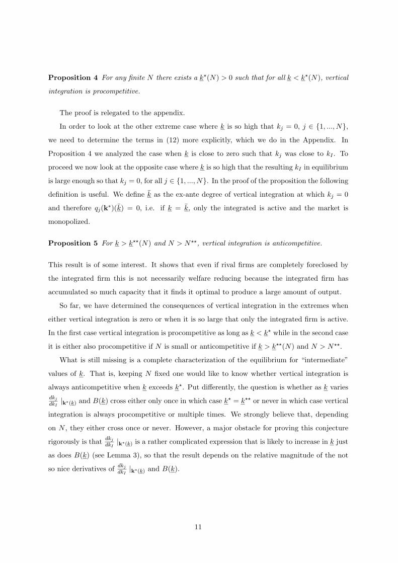
Proposition 4 For any finite N there exists a k?(N) > 0 such that for all k < k?(N), vertical
integration is procompetitive.
The proof is relegated to the appendix.
In order to look at the other extreme case where k is so high that kj = 0, j ∈ {1, ..., N},we need to determine the terms in (12) more explicitly, which we do in the Appendix. In
Proposition 4 we analyzed the case when k is close to zero such that kj was close to kI . To
proceed we now look at the opposite case where k is so high that the resulting kI in equilibrium
is large enough so that kj = 0, for all j ∈ {1, ..., N}. In the proof of the proposition the following
definition is useful. We define k as the ex-ante degree of vertical integration at which kj = 0
and therefore qj(k∗)(k) = 0, i.e. if k = k, only the integrated is active and the market is
monopolized.
Proposition 5 For k > k??(N) and N > N??, vertical integration is anticompetitive.
This result is of some interest. It shows that even if rival firms are completely foreclosed by
the integrated firm this is not necessarily welfare reducing because the integrated firm has
accumulated so much capacity that it finds it optimal to produce a large amount of output.
So far, we have determined the consequences of vertical integration in the extremes when
either vertical integration is zero or when it is so large that only the integrated firm is active.
In the first case vertical integration is procompetitive as long as k < k? while in the second case
it is either also procompetitive if N is small or anticompetitive if k > k??(N) and N > N??.
What is still missing is a complete characterization of the equilibrium for “intermediate”
values of k. That is, keeping N fixed one would like to know whether vertical integration is
always anticompetitive when k exceeds k?. Put differently, the question is whether as k variesdkj
dkI|k∗(k) and B(k) cross either only once in which case k? = k?? or never in which case vertical
integration is always procompetitive or multiple times. We strongly believe that, depending
on N , they either cross once or never. However, a major obstacle for proving this conjecture
rigorously is that dkj
dkI|k∗(k) is a rather complicated expression that is likely to increase in k just
as does B(k) (see Lemma 3), so that the result depends on the relative magnitude of the not
so nice derivatives of dkj
dkI|k∗(k) and B(k).
11
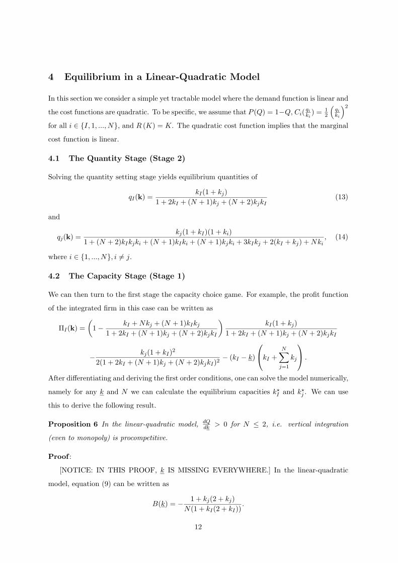
4 Equilibrium in a Linear-Quadratic Model
In this section we consider a simple yet tractable model where the demand function is linear and
the cost functions are quadratic. To be specific, we assume that P (Q) = 1−Q, Ci( qiki
) = 12
(qiki
)2
for all i ∈ {I, 1, ..., N}, and R (K) = K. The quadratic cost function implies that the marginal
cost function is linear.
4.1 The Quantity Stage (Stage 2)
Solving the quantity setting stage yields equilibrium quantities of
qI(k) =kI(1 + kj)
1 + 2kI + (N + 1)kj + (N + 2)kjkI(13)
and
qj(k) =kj(1 + kI)(1 + ki)
1 + (N + 2)kIkjki + (N + 1)kIki + (N + 1)kjki + 3kIkj + 2(kI + kj) + Nki, (14)
where i ∈ {1, ..., N}, i 6= j.
4.2 The Capacity Stage (Stage 1)
We can then turn to the first stage the capacity choice game. For example, the profit function
of the integrated firm in this case can be written as
ΠI(k) =(
1− kI + Nkj + (N + 1)kIkj
1 + 2kI + (N + 1)kj + (N + 2)kjkI
)kI(1 + kj)
1 + 2kI + (N + 1)kj + (N + 2)kjkI
− kj(1 + kI)2
2(1 + 2kI + (N + 1)kj + (N + 2)kjkI)2− (kI − k)
kI +
N∑
j=1
kj
.
After differentiating and deriving the first order conditions, one can solve the model numerically,
namely for any k and N we can calculate the equilibrium capacities k?I and k?
j . We can use
this to derive the following result.
Proposition 6 In the linear-quadratic model, dQdk > 0 for N ≤ 2, i.e. vertical integration
(even to monopoly) is procompetitive.
Proof :
[NOTICE: IN THIS PROOF, k IS MISSING EVERYWHERE.] In the linear-quadratic
model, equation (9) can be written as
B(k) = − 1 + kj(2 + kj)N(1 + kI(2 + kI))
.
12

Thus, if vertical integration yields a monopoly and kj = 0 we have
B(k) = − 1N(1 + kI(2 + kI))
. (15)
Calculating dkj
dkIfor the case kj = 0 gives
dkj
dkI|kj=0= − 2 + kI(7 + 12kI + 8k2
I )(1 + N)(2 + 3kI)(1 + 3kI(1 + kI))
. (16)
Subtracting (15) from (16) gives
−NkI(2 + 13kI + 28k2I + 30k3
I + 8k4I )− 2− kI(9 + 15kI + 9k2
I )(1 + N)(2 + 3kI)(1 + 3kI(1 + kI))N(1 + kI)2
.
We can use this expression and check if it is greater than zero at the equilibrium value of kI
at which kj = 0. For the case of N = 2 we get that k = 0.41655 induces kI = 0.32305 which
yields kj = 0. With N = 3 and kI = 0.32305 the expression is 0.00115 > 0 and so vertical
integration to monopoly is procompetitive. On the other hand, for N ≥ 3, vertical integration
yields a negative expression. ¥
The above result might look surprising at first glance because it implies that one large
firm is better for consumers than an oligopoly consisting of three firms. Yet, the result can
be explained by the fact that our model does explicitly take into account efficiency gains in
production that go beyond pure avoidance of double marginalization. To push its competitors
out of the market, a firm must acquire a large amount of capacity with which it will produce a
quantity that is larger than the oligopoly quantity. Thus, our model implies a more permissive
handle of vertical integration than previous ones.
5 Conclusions
In this paper we show that vertical integration with a downstream oligopoly and an increasing
upstream supply curve is procompetitive under a fairly wide circumstances. Whether it is
procompetitive or anticompetitive depends on the degree of ex ante vertical integration. Only
if this degree is high and the number of downstream competitors relatively large will vertical
integration reduce final goods output and increase consumer prices. Otherwise, vertical inte-
gration lowers prices and thus benefits consumers. These predictions differ starkly from the
dominant firm model. Consequently, it would be misleading to extrapolate these results to
models with a different, and in some sense more general, downstream market structure.
An interesting extension of the model, suggested by Rey and Tirole (2007), is to endogenize
k. Our model makes clear predictions under which vertical integration is procompetitive, yet
13
it does not determine the optimal, or equilibrium, degree of vertical integration, assuming that
the vertically integrated firm has to pay to acquire capacity. Such an analysis is not possible
in the dominant firm model because there the dominant firm is the only one who can acquire
capacity at the upstream market. The present model with downstream oligopoly provides a
framework that permits an analysis of the question whether the amount of capacity acquired
in equilibrium is indeed small enough for vertical integration to be procompetitive. This is
something we plan to analyze in the near future.
A Appendix
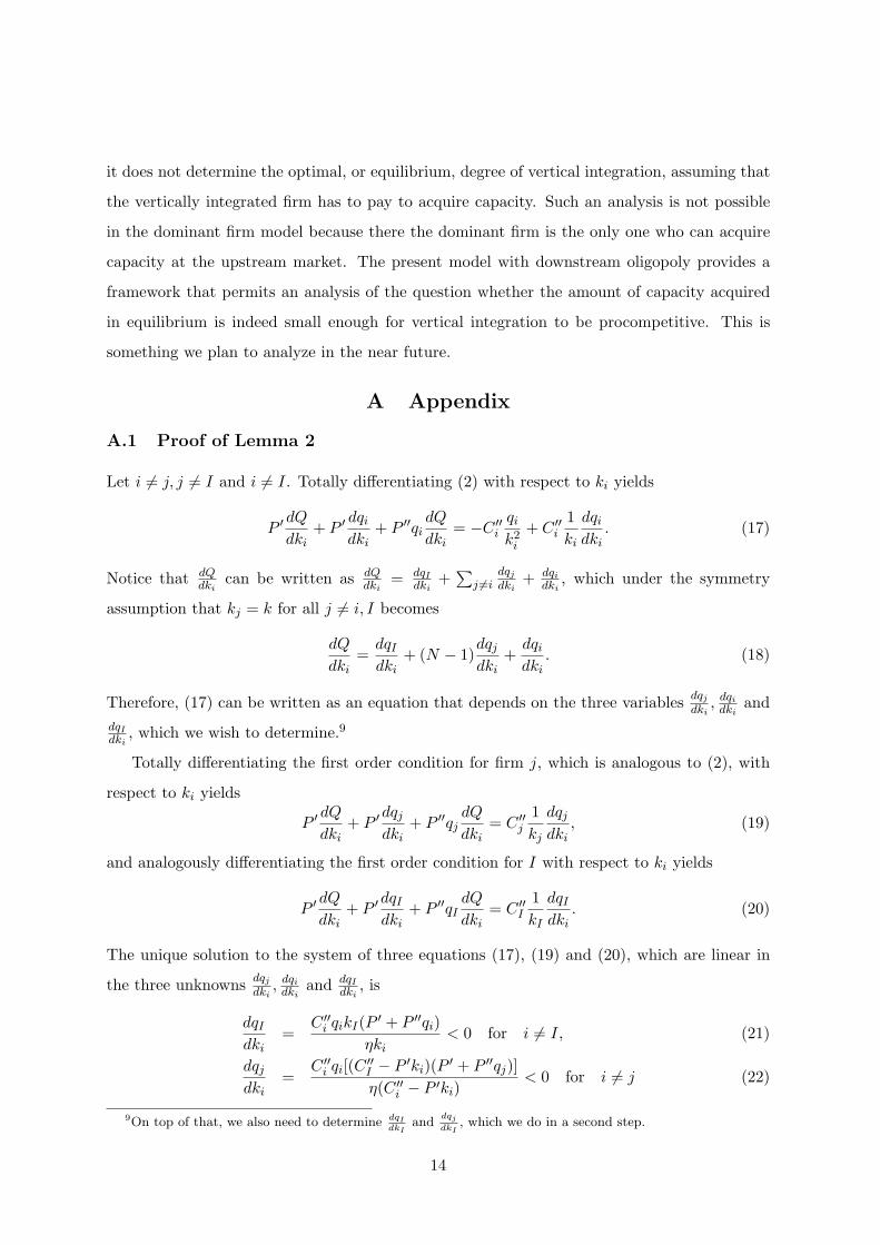
A.1 Proof of Lemma 2
Let i 6= j, j 6= I and i 6= I. Totally differentiating (2) with respect to ki yields
P ′ dQ
dki+ P ′ dqi
dki+ P ′′qi
dQ
dki= −C ′′
i
qi
k2i
+ C ′′i
1ki
dqi
dki. (17)
Notice that dQdki
can be written as dQdki
= dqIdki
+∑
j 6=idqj
dki+ dqi
dki, which under the symmetry
assumption that kj = k for all j 6= i, I becomes
dQ
dki=
dqI
dki+ (N − 1)
dqj
dki+
dqi
dki. (18)
Therefore, (17) can be written as an equation that depends on the three variables dqj
dki, dqi
dkiand
dqIdki
, which we wish to determine.9
Totally differentiating the first order condition for firm j, which is analogous to (2), with
respect to ki yields
P ′ dQ
dki+ P ′dqj
dki+ P ′′qj
dQ
dki= C ′′
j
1kj
dqj
dki, (19)
and analogously differentiating the first order condition for I with respect to ki yields
P ′ dQ
dki+ P ′dqI
dki+ P ′′qI
dQ
dki= C ′′
I
1kI
dqI
dki. (20)
The unique solution to the system of three equations (17), (19) and (20), which are linear in
the three unknowns dqj
dki, dqi
dkiand dqI
dki, is
dqI
dki=
C ′′i qikI(P ′ + P ′′qi)
ηki< 0 for i 6= I, (21)
dqj
dki=
C ′′i qi[(C ′′
I − P ′ki)(P ′ + P ′′qj)]η(C ′′
i − P ′ki)< 0 for i 6= j (22)
9On top of that, we also need to determine dqIdkI
anddqj
dkI, which we do in a second step.
14
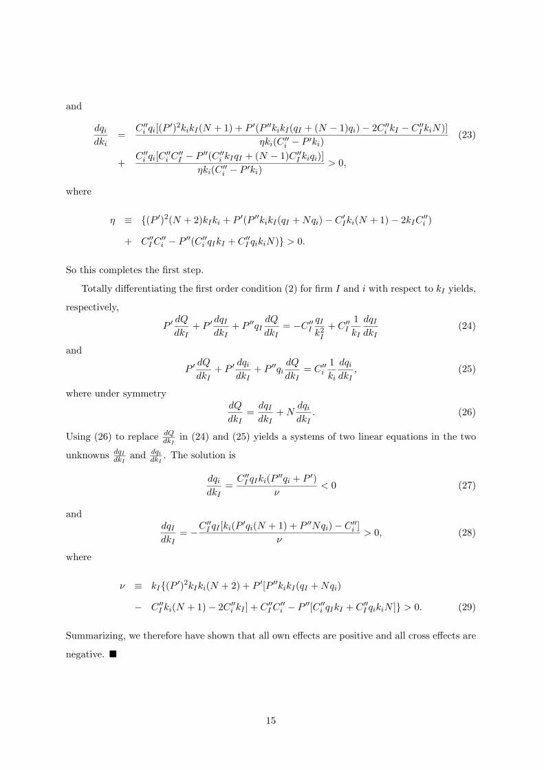
and
dqi
dki=
C ′′i qi[(P ′)2kikI(N + 1) + P ′(P ′′kikI(qI + (N − 1)qi)− 2C ′′
i kI − C ′′I kiN)]
ηki(C ′′i − P ′ki)
(23)
+C ′′
i qi[C ′′i C ′′
I − P ′′(C ′′i kIqI + (N − 1)C ′′
I kiqi)]ηki(C ′′
i − P ′ki)> 0,
where
η ≡ {(P ′)2(N + 2)kIki + P ′(P ′′kikI(qI + Nqi)− C ′Iki(N + 1)− 2kIC
′′i )
+ C ′′I C ′′
i − P ′′(C ′′i qIkI + C ′′
I qikiN)} > 0.
So this completes the first step.
Totally differentiating the first order condition (2) for firm I and i with respect to kI yields,
respectively,
P ′ dQ
dkI+ P ′ dqI
dkI+ P ′′qI
dQ
dkI= −C ′′
I
qI
k2I
+ C ′′I
1kI
dqI
dkI(24)
and
P ′ dQ
dkI+ P ′ dqi
dkI+ P ′′qi
dQ
dkI= C ′′
i
1ki
dqi
dkI, (25)
where under symmetrydQ
dkI=
dqI
dkI+ N
dqi
dkI. (26)
Using (26) to replace dQdkI
in (24) and (25) yields a systems of two linear equations in the two
unknowns dqIdkI
and dqi
dkI. The solution is
dqi
dkI=
C ′′I qIki(P ′′qi + P ′)
ν< 0 (27)
anddqI
dkI= −C ′′
I qI [ki(P ′qi(N + 1) + P ′′Nqi)− C ′′i ]
ν> 0, (28)
where
ν ≡ kI{(P ′)2kIki(N + 2) + P ′[P ′′kikI(qI + Nqi)
− C ′′I ki(N + 1)− 2C ′′
i kI ] + C ′′I C ′′
i − P ′′[C ′′i qIkI + C ′′
I qikiN ]} > 0. (29)
Summarizing, we therefore have shown that all own effects are positive and all cross effects are
negative. ¥
15

A.2 Proof of Proposition 1
The profit function at the capacity stage for the integrated firm is
ΠI(k) = P (Q(k))qI(k)− kIC
(qI(k)kI
)− (kI − k)R
kI +
N∑
j=1
kj
. (30)
Using the envelope theorem and dropping arguments, the capacity first order condition for the
integrated firm is
P ′dQ−I
dkIqI − CI + C ′
I
qI
kI−R− (kI − k)R′ = 0, (31)
where Q−I is the aggregate equilibrium quantity of all firms other than I, i.e. Q−I ≡∑N
j=1 qj .
The profit function by a representative non-integrated firm j is given by
Πj(k) = P (Q(k))qj(k)− kjC
(qj(k)kj
)− kjR
kI +
N∑
j=i
ki
(32)
and the first order condition is
P ′dQ−j
dkjqj − Cj + C ′
j
qj
kj−R− kjR
′ = 0. (33)
Differentiating (31) and (33) with respect to k yields
∂2ΠI
∂k2I
dkI
dk+ N
∂2ΠI
∂kI∂kj
dkj
dk+
∂2ΠI
∂kI∂k= 0
and∂2Πj
∂k2j
dkj
dk+ (N − 1)
∂2Πj
∂kj∂ki
dki
dk+
∂2Πj
∂kj∂kI
dkI
dk= 0.
Using the fact that in equilibrium dkIdk = dkj
dk we get
dkj
dk=
∂2Πj
∂kj∂kI
∂2ΠI∂kI∂k
∂2Πj
∂k2j
∂2ΠI
∂k2I
+ (N − 1) ∂2Πj
∂kj∂ki
∂2ΠI
∂k2I−N
∂2Πj
∂kj∂kI
∂2ΠI∂kI∂kj
(34)
and
dkj
dk= −
∂2ΠI∂kI∂k
(∂2Πj
∂k2j
+ (N − 1) ∂2Πj
∂kj∂ki
)
∂2Πj
∂k2j
∂2ΠI
∂k2I
+ (N − 1) ∂2Πj
∂kj∂ki
∂2ΠI
∂k2I−N
∂2Πj
∂kj∂kI
∂2ΠI∂kI∂kj
. (35)
Since we can ignore terms with P ′′, the six terms that determine the fractions of the last
16

equations can be written as
∂2Πj
∂k2j
= P ′ dqj
dkj
[dqI
dkj+ (N − 1)
dqi
dkj
]+ P ′qj
[d2qI
dk2j
+ (N − 1)d2qi
dk2j
]
+ C ′′j
qj
k2j
(dqj
dkj− qj
kj
)− 2R′ − kjR
′′, (36)
∂2Πj
∂kj∂kI= P ′ dqj
dkI
[dqI
dkj+ (N − 1)
dqi
dkj
]+ P ′qj
[d2qI
dkjdkI+ (N − 1)
d2qi
dkjdkI
]
+ C ′′j
qj
k2j
dqj
dkI−R′ − kjR
′′, (37)
∂2Πj
∂kj∂ki= P ′dqj
dki
[dqI
dkj+ (N − 1)
dqi
dkj
]+ P ′qj
[d2qI
dkjdki+ (N − 2)
d2qk
dkjdki+
d2qi
dkjdki
]
+ C ′′j
qj
k2j
dqj
dki−R′ − kjR
′′, (38)
∂2ΠI
∂k2I
= P ′ dqI
dkIN
dqj
dkI+ P ′qIN
d2qj
dk2I
+ C ′′I
qI
k2I
(dqI
dkI− qI
kI
)− 2R′ − (kI − k)R′′, (39)
∂2ΠI
∂kI∂kj= P ′ dqI
dkjN
dqj
dkI+ P ′qI
[d2qj
dkjdkI+ (N − 1)
d2qi
dkjdkI
]
+ C ′′I
qI
k2I
dqI
dkI−R′ − (kI − k)R′′, (40)
∂2ΠI
∂kI∂k= +R′. (41)
From the proof of Lemma 2 we know all the expressions containing first derivatives. From these
expressions we can determine the expression for the ten second derivatives that are present in
the last equations. These expressions are the following:
d2qI
dk2j
= 2kI(P ′)2C ′′
j qj
[−kIkj (2 + N) (P ′)2 +
(3kIC
′′j + C ′′
I kj (1 + N))
P ′ − 2C ′′j C ′′
I
]
kj
[−kIkj (2 + N) (P ′)2 +
(C ′′
I kj (1 + N) + 2kIC ′′j
)P ′ − C ′′
j C ′′I
]2 (−C ′′
j + kjP ′) > 0,
d2qj
dk2j
= −2qjC
′′j (C ′′
I − kIP′)(P ′)2
[−kIkj (2 + N) (P ′)2 +
(3kIC
′′j + C ′′
I kj (1 + N))
P ′ − 2C ′′j C ′′
I
]
[−kIkj (2 + N) (P ′)2 +
(C ′′
I kj (1 + N) + 2kIC ′′j
)P ′ − C ′′
j C ′′I
]2 (−C ′′
j + kjP ′)2 > 0,
d2qI
dkjdkI=
P ′C ′′j C ′′
I
(qjC
′′j − P ′kj(−qI + qj(N + 1))
)
kj
((P ′)2kjkI(2 + N)− (2kIC ′′
j + kj(1 + N)C ′′I )P ′ + C ′′
j C ′′I
)2 ,
d2qi
dkjdkI=
(P ′)2C ′′j C ′′
I (−kIkj(qI + qj)P ′ + C ′′j qjkI + C ′′
I qIkj)
kI(C ′′j − kjP ′)
(kIkj(N + 2)(P ′)2 − ((1 + N)kjC ′′
I + 2kjC ′′j )P ′ + C ′′
j C ′′I
)2 > 0,
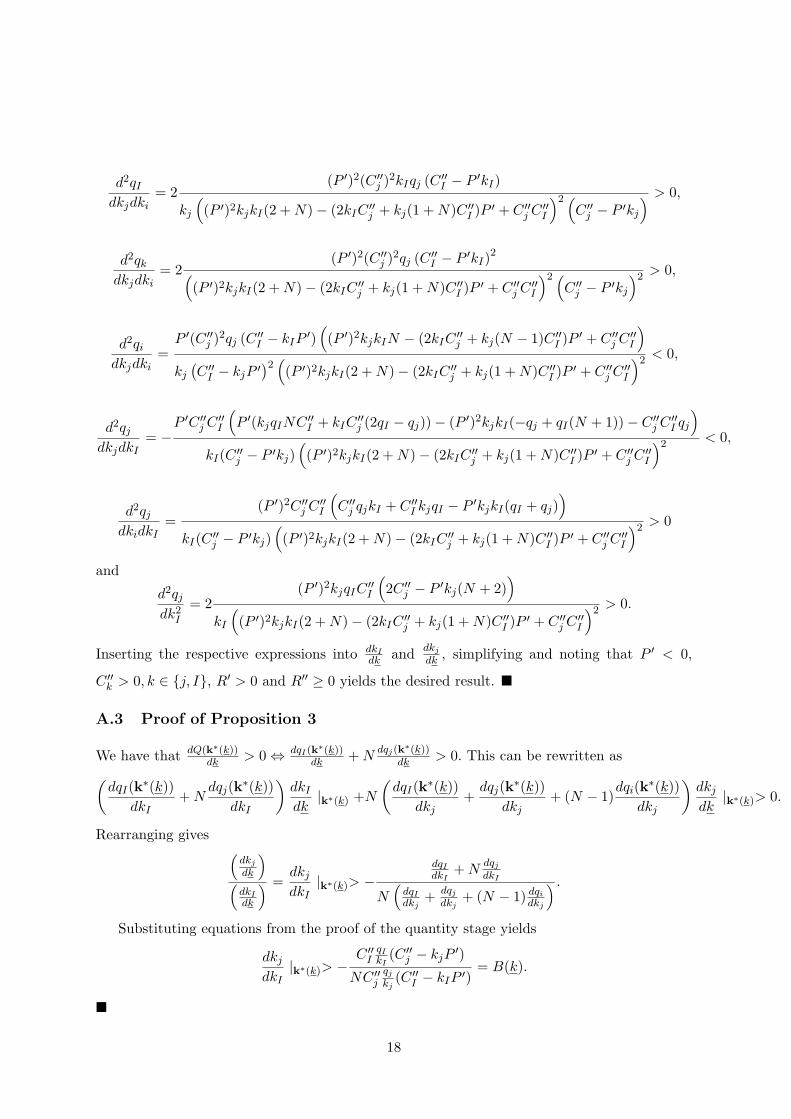
17
d2qI
dkjdki= 2
(P ′)2(C ′′j )2kIqj (C ′′
I − P ′kI)
kj
((P ′)2kjkI(2 + N)− (2kIC ′′
j + kj(1 + N)C ′′I )P ′ + C ′′
j C ′′I
)2 (C ′′
j − P ′kj
) > 0,
d2qk
dkjdki= 2
(P ′)2(C ′′j )2qj (C ′′
I − P ′kI)2
((P ′)2kjkI(2 + N)− (2kIC ′′
j + kj(1 + N)C ′′I )P ′ + C ′′
j C ′′I
)2 (C ′′
j − P ′kj
)2 > 0,
d2qi
dkjdki=
P ′(C ′′j )2qj (C ′′
I − kIP′)
((P ′)2kjkIN − (2kIC
′′j + kj(N − 1)C ′′
I )P ′ + C ′′j C ′′
I
)
kj
(C ′′
I − kjP ′)2((P ′)2kjkI(2 + N)− (2kIC ′′
j + kj(1 + N)C ′′I )P ′ + C ′′
j C ′′I
)2 < 0,
d2qj
dkjdkI= −
P ′C ′′j C ′′
I
(P ′(kjqINC ′′
I + kIC′′j (2qI − qj))− (P ′)2kjkI(−qj + qI(N + 1))− C ′′
j C ′′I qj
)
kI(C ′′j − P ′kj)
((P ′)2kjkI(2 + N)− (2kIC ′′
j + kj(1 + N)C ′′I )P ′ + C ′′
j C ′′I
)2 < 0,
d2qj
dkidkI=
(P ′)2C ′′j C ′′
I
(C ′′
j qjkI + C ′′I kjqI − P ′kjkI(qI + qj)
)
kI(C ′′j − P ′kj)
((P ′)2kjkI(2 + N)− (2kIC ′′
j + kj(1 + N)C ′′I )P ′ + C ′′
j C ′′I
)2 > 0
and
d2qj
dk2I
= 2(P ′)2kjqIC
′′I
(2C ′′
j − P ′kj(N + 2))
kI
((P ′)2kjkI(2 + N)− (2kIC ′′
j + kj(1 + N)C ′′I )P ′ + C ′′
j C ′′I
)2 > 0.
Inserting the respective expressions into dkIdk and dkj
dk , simplifying and noting that P ′ < 0,
C ′′k > 0, k ∈ {j, I}, R′ > 0 and R′′ ≥ 0 yields the desired result. ¥
A.3 Proof of Proposition 3
We have that dQ(k∗(k))dk > 0 ⇔ dqI(k∗(k))
dk + Ndqj(k
∗(k))dk > 0. This can be rewritten as
(dqI(k∗(k))
dkI+ N
dqj(k∗(k))dkI
)dkI
dk|k∗(k) +N
(dqI(k∗(k))
dkj+
dqj(k∗(k))dkj
+ (N − 1)dqi(k∗(k))
dkj
)dkj
dk|k∗(k)> 0.
Rearranging gives(
dkj
dk
)(
dkIdk
) =dkj
dkI|k∗(k)> −
dqIdkI
+ Ndqj
dkI
N(
dqIdkj
+ dqj
dkj+ (N − 1) dqi
dkj
) .
Substituting equations from the proof of the quantity stage yields
dkj
dkI|k∗(k)> −
C ′′I
qIkI
(C ′′j − kjP
′)
NC ′′j
qj
kj(C ′′
I − kIP ′)= B(k).
¥
18

A.4 Proof of Lemma 3
From Corollary 3 we know that qhkh
decreases in kh and Proposition 1 says that kI > kj anddkIdk > 0. Therefore, we can write kj = a(k)kI , with 0 ≤ a(k) ≤ 1, qj/kj = b(k)(qI/kI) with
b(k) > 1 and C ′′j = d(k)C ′′
I with d(k) > 1. Since dkj/dkI < 0 (because of the assumption that
a unique pure strategy equilibrium exists), it follows that a′ < 0, b′ > 0 and d′ > 0.
Substituting these into (9) yields
B = −C ′′
IqIkI
(C ′′j − kjP
′)
NC ′′j
qj
kj(C ′′
I − kIP ′)= − 1
N
d(k)C ′′I − a(k)kIP
′
b(k)d(k)(C ′′I − kIP ′)
> − 1N
, (42)
where the inequality follows because b(k)d(k) > 1 > a(k) ≥ 0 holds, so that the second fraction
is positive but less than 1. Dropping all arguments, one gets
dB
dk= − 1
N
−a′bdkIP′ + abd′kIP
′ + ab′dkIP′ − d2b′C ′′
I
(bd)2(C ′′
I − kIP ′) > 0. (43)
¥
A.5 Proof of Proposition 4
Preliminaries. Dividing dkIdk |k∗(k) by dkj
dk |k∗(k) from Proposition 1 yields
dkj
dk |k∗(k)
dkIdk |k∗(k)
=dkj
dkI|k∗(k)= − ξ − φ(R′ + kjR
′′)ψ − φ((N + 1)R′ + NkjR′′)
,
with
ξ = kjqjqIC′′j C ′′
I×[(P ′)5k3
j kI
(3N + 2− 2
qj
qI
)− (P ′)4k2
j
(C ′′
j kI
(4N + 8− 5
qj
qI
)+ C ′′
I kj(3N − 1))−
+(P ′)3kjC′′j
(C ′′
j kI
(N + 8− 4
qj
qI
)+ C ′′
I kj(4N + 1))− (44)
−(P ′)2(C ′′j )2
(C ′′
j kI
(2− qj
qI
)+ C ′′
I kj(N + 3))
+ P ′(C ′′j )3C ′′
I
]< 0,
ψ = kIq2j C
′′j
[−(P ′)6k3
j k2I (N+2)(3N+2)+(P ′)5k2
j kI
(C ′′
j kI(18 + 13N + 3N2) + 2C ′′I Nkj(5 + 3N)
)−
−(P ′)4kj
((C ′′
j )2k2I (16 + 6N + N2) + C ′′
j C ′′I kjkI(15 + 17N + 6N2) + 2(C ′′
I )2(N + 1)k2j (3N − 1)
)+
+(P ′)3C ′′j
(2(C ′′
j )2k2I (N + 1) + C ′′
j C ′′I kjkI(9 + 4N + N2) + 2(C ′′
I )2k2j (3 + 4N + N2)
)−
19

−(P ′)2(C ′′
j )2C ′′I (3C ′′
j kI(N + 1) + 2(C ′′I )2k2
j (5 + 2N + N2))+P ′(C ′′
j )3(C ′′I )2(N +1)
]< 0, (45)
and
φ = kIk2j (C
′′j − kjP
′)2((P ′)2kjkI(N + 2)− P ′(2C ′′
j kI + C ′′I kj(N + 1)) + C ′′
j C ′′I
)2> 0.
Assume now that ex ante there is no vertical integration (k = 0), so that k∗I = k∗j ,
qI(k∗(k)) = qj(k∗(k)), and C ′′I = C ′′
j . In this case
B(0) = − 1N
.
On the other hand, in the expression for dkj
dkI|k∗(k), we get
ξ = −q2j P
′(C ′′j )2(C ′′
j − kjP′)2(3(P ′)2k2
j N − P ′kjC′′j N + (C ′′
j )2),
ψ = −q2j P
′C ′′j (C ′′
j − kjP′)2
((P ′)3k3
j (N + 2)(3N + 2)− (P ′)2k2j C
′′j (10 + 3N2 + 7N)+
+P ′kj(C ′′j )2(6 + N2 + 3N)− (N + 1)(C ′′
j )3)
and
φ = kIk2j (C
′′j − kjP
′)4(C ′′j − (N + 2)kjP
′)2.
Subtracting B from dkj
dkI|k∗(k) at k = 0 yields that
dkj
dkI|k∗(k) −B > 0,
if and only if
R′k2j (C
′′j − kjP
′)4(C ′′j − (N + 2)kjP
′)2−
−q2j C
′′j P ′(C ′′
j − kjP′)2(C ′′
j − (N + 2)kjP′)((P ′)2k2
j (3N + 1)− 4P ′kjC′′j + (C ′′
j )2) > 0.
But obviously the last inequality is always satisfied since P ′ < 0 and C ′′j > 0. Thus, at k = 0
vertical integration is consumer welfare increasing. ¥
20
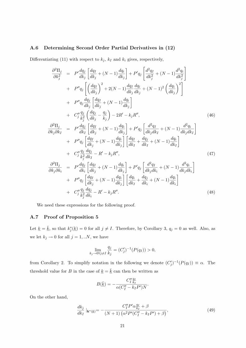
A.6 Determining Second Order Partial Derivatives in (12)
Differentiating (11) with respect to kj , kI and ki gives, respectively,
∂2Πj
∂k2j
= P ′ dqj
dkj
[dqI
dkj+ (N − 1)
dqi
dkj
]+ P ′qj
[d2qI
dk2j
+ (N − 1)d2qi
dk2j
]
+ P ′′qj
[(dqI
dkj
)2
+ 2(N − 1)dqI
dkj
dqi
dkj+ (N − 1)2
(dqi
dkj
)2]
+ P ′′qjdqj
dkj
[dqI
dkj+ (N − 1)
dqi
dkj
]
+ C ′′j
qj
k2j
(dqj
dkj− qj
kj
)− 2R′ − kjR
′′, (46)
∂2Πj
∂kj∂kI= P ′ dqj
dkI
[dqI
dkj+ (N − 1)
dqi
dkj
]+ P ′qj
[d2qI
dkjdkI+ (N − 1)
d2qi
dkjdkI
]
+ P ′′qj
[dqI
dkj+ (N − 1)
dqi
dkj
] [dqI
dkI+
dqj
dkI+ (N − 1)
dqi
dkI
]
+ C ′′j
qj
k2j
dqj
dkI−R′ − kjR
′′, (47)
∂2Πj
∂kj∂ki= P ′dqj
dki
[dqI
dkj+ (N − 1)
dqi
dkj
]+ P ′qj
[d2qI
dkjdki+ (N − 1)
d2qi
dkjdki
]
+ P ′′qj
[dqI
dkj+ (N − 1)
dqi
dkj
] [dqi
dkI+
dqj
dki+ (N − 1)
dqi
dki
]
+ C ′′j
qj
k2j
dqj
dki−R′ − kjR
′′. (48)
We need these expressions for the following proof.
A.7 Proof of Proposition 5
Let k = k, so that k∗j (k) = 0 for all j 6= I. Therefore, by Corollary 3, qj = 0 as well. Also, as
we let kj → 0 for all j = 1, ..N , we have
limkj→0∀j 6=I
qj
kj= (C ′
j)−1(P (qI)) > 0,
from Corollary 2. To simplify notation in the following we denote (C ′j)−1(P (qI)) ≡ α. The
threshold value for B in the case of k = k can then be written as
B(k) = −C ′′
IqIkI
α(C ′′I − kIP ′)N
.
On the other hand,
dkj
dkI|k∗(k)= −
C ′′I P ′α qI
kI+ β
(N + 1)(α2P ′(C ′′
I − kIP ′) + β) , (49)
21

with β ≡ R′kI (2P ′kI − C ′′I ) < 0. It follows that
dkj
dkI|k∗(k)< B(k)
if and only if
−(
N
1 + N
)C ′′
I P ′α qIkI
+ β
α2P ′(C ′′I − kIP ′) + β
< −C ′′
IqIkI
α(C ′′I − kIP ′)
. (50)
If N → ∞, N/(1 + N) → 1. In this case the left hand side of (50) is smaller than the right
hand side. To see this, notice that − C′′I P ′α qIkI
+β
α2P ′(C′′I −kIP ′)+β= − C′′I
qIkI
α(C′′I −kIP ′) if and only if β = 0. But
since β < 0, the left hand side is smaller than the right hand side. Conversely, if N is small
the right hand side can either be larger or smaller than the left hand side dependent on the
exact functional forms. As a result we have that if k = k an increase in k can either be pro -
or anticompetitive. ¥
References
Chen, Y.-M. (2001): “On Vertical Mergers and their Competitive Effects,” RAND Journal
of Economics, 32, 667–685.
Choi, J.-P., and S.-S. Yi (2000): “Vertical Foreclosure with the Choice of Input Specifica-
tions,” RAND Journal of Economics, 31, 717–743.
Hart, O., and J. Tirole (1990): “Vertical Integration and Market Foreclosure,” Brookings
Papers on Economic Activity: Microeconomics, pp. 205–276.
Hendricks, K., and R. McAfee (2007): “Theory of Bilateral Oligopoly,” Working Paper,
California Institute of Technology.
Hortacsu, A., and C. Syverson (2007): “Cementing Relationships: Vertical Integration,
Foreclosure, Productivity, and Prices,” Journal of Political Economy, 115, 250–301.
Klemperer, P., and M. Meyer (1989): “Supply Function Equilibria in Oligopoly under
Uncertainty,” Econometrica, 57, 1243–1277.
Ordover, J. A., G. Saloner, and S. C. Salop (1990): “Equilibrium Vertical Foreclosure,”
American Economic Review, 71, 127–42.
Perry, M. K. (1978): “Vertical Integration: The Monopsony Case,” American Economic
Review, 68(4), 561–70.
22
Rey, P., and J. Tirole (2007): “A Primer on Foreclosure,” in: Handbook of Industrial
Organization, Vol. 3, eds.: M. Armstrong and R.H. Porter, Elsevier B.V., North Holland,
Amsterdam, pp. 2145–2220.
Riordan, M. H. (1998): “Anticompetitive Vertical Integration by a Dominant Firm,” Amer-
ican Economic Review, 88, 1232–48.
(2008): “Competitive Effects of Vertical Integration,” Handbook of Antitrust Eco-
nomics.
Salinger, M. A. (1988): “Vertical Mergers and Market Foreclosure,” Quarterly Journal of
Eonomics, 103, 345–56.
23