Competition, Productivity, and Trade, Reconsidered— JSIE Annual Meetings —

Tomohiro Ara

Fukushima Univ

October 18, 2020

Motivation

■ Country size has a critical impact on domestic/export shares:

◦ A large (small) country tends to have a large (small) domestic share of

expenditure

◦ Most firms provide their products for the domestic market in a large country,

while a large fraction of firms export in a small country

⇒ Country size seems to have selection effects that are opposite to trade

liberalization in a country of origin

Motivation (cont.)

Putting Ricardo to Work 81

Table 2 reports the home share in 2006 for the 25 countries with data on Table 2 reports the home share in 2006 for the 25 countries with data on gross manufacturing production. The mean value of the home share is just under gross manufacturing production. The mean value of the home share is just under 50 percent. In a world of frictionless trade (all 50 percent. In a world of frictionless trade (all dnini == 1), there is no reason for a 1), there is no reason for a country to spend a larger share of its income on its own goods than any other country to spend a larger share of its income on its own goods than any other country. A country’s home share, in that case, would correspond to its share in country. A country’s home share, in that case, would correspond to its share in world output. As Table 2 makes clear, for each of these countries the home share world output. As Table 2 makes clear, for each of these countries the home share is many times larger than the country’s share in world GDP: three times higher for is many times larger than the country’s share in world GDP: three times higher for the United States, ten times for Germany, 50 times for Denmark, and 100 times for the United States, ten times for Germany, 50 times for Denmark, and 100 times for Greece. Such multiples illustrate the extent to which trade barriers continue to chop Greece. Such multiples illustrate the extent to which trade barriers continue to chop up world markets. Even though countries buy much more of their manufactures up world markets. Even though countries buy much more of their manufactures

Table 2The Home Share of Spending on Manufactures and Gains from Trade

World GDPshare (%) in

2006

Home share of spending Implied gains from trade

CountryLevel in

2006 (%)Change since 1996 (percentage points)

Level in 2006 (%)

Change since 1996 (percentage points)

Austria 0.66 31.4 –16.2 21.3 8.1Canada 2.60 49.1 –1.5 12.6 0.6Czech Republic 0.29 42.6 –14.7 15.3 5.5Denmark 0.56 25.6 –18.1 25.5 10.7Estonia 0.03 2.5 –19.6 85.4 56.7Finland 0.42 58.2 –7.3 9.4 2.1France 4.60 56.9 –10.3 9.9 3.0Germany 5.94 53.7 –16.4 10.9 4.8Greece 0.54 52.7 –11.6 11.3 3.6Hungary 0.23 26.0 –34.5 25.1 16.4Iceland 0.03 27.9 –10.0 23.7 6.2Ireland 0.46 39.6 9.9 16.7 –5.7Italy 3.80 68.9 –7.1 6.4 1.7Japan 8.88 84.9 –5.6 2.8 1.1Korea 1.94 77.2 –0.7 4.4 0.1Mexico 1.94 58.3 –7.9 9.4 2.3New Zealand 0.22 53.6 –8.2 11.0 2.6Norway 0.68 51.9 –2.5 11.6 0.9Poland 0.69 53.4 –15.8 11.0 4.7Portugal 0.41 50.8 –10.2 12.0 3.4Slovenia 0.08 27.2 –15.5 24.3 9.0Spain 2.51 62.8 –10.2 8.1 2.7Sweden 0.81 49.2 –10.0 12.5 3.4Switzerland 0.80 35.3 –20.0 18.9 8.6United States 27.26 73.5 –8.3 5.3 1.9All others 33.62

Source: Authors’ calculations from the OECD STAN (STructural ANalysis) Database, the Economist Intelligence Unit, and a model described in the text.Notes: The home share is the share a country spends on domestic manufactures out of total country spending on manufactures. The last two columns calculate the implications of the level of the home share, and its changes over time, for countries’ gains from trade and how those gains have evolved. We look at the gains from trade only in manufactures.

Source: Eaton and Kortum (2011)

Motivation (cont.)

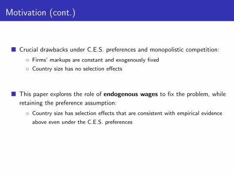
■ Crucial drawbacks under C.E.S. preferences and monopolistic competition:

◦ Firms’ markups are constant and exogenously fixed

◦ Country size has no selection effects

■ This paper explores the role of endogenous wages to fix the problem, while

retaining the preference assumption:

◦ Country size has selection effects that are consistent with empirical evidence

above even under the C.E.S. preferences

Motivation (cont.)

■ Why does country size matter in endogenous wages?:

◦ p(φ)c(φ)

= σσ−1

(markups)

◦ p(φ)− c(φ) = 1σ−1

wφ

(price-cost margins)

◦ L ↑ ⇒ w ↑ ⇒ p(φ)− c(φ) ↑ ⇒ φ∗d ↓, φ∗

x ↑

■ Caveats:

◦ Channel is not operative if wages are exogenously fixed by a freely tradable

“outside” good

◦ The result does not depend on the above two specifications, but depends on

endogenous wages

Motivation (cont.)

■ Why should we care about the country size effect?:

◦ The model predicts a large country accommodates relatively inefficient firms in

the domestic market

◦ While a larger country can enjoy terms-of-trade gains by setting higher tariffs,

this also accelerates welfare losses from protecting inefficient firms

⇒ A larger country does not always benefit from higher tariffs

Related literature

■ Demidova and Rodrıguez-Clare (2013):

◦ Endogenous wages can reverse the impact of trade liberalization on welfare in

a unilaterally liberalizing country

◦ Country size is used to obtain the equilibrium outcome for a small economy

■ Melitz and Ottaviano (2008):

◦ A country with larger size entails higher productivity and welfare, reducing

firms’ average markups

◦ Due to an outside good, trade liberalization can result in a welfare loss

Roadmap

■ Model setup

■ Impact of trade liberalization:

◦ Welfare gains in a unilaterally liberalizing country

■ Impact of country size:

◦ Higher price-cost margins in a larger country

◦ Entry that is not proportional to country size

■ Summary

Model

■ Melitz (2003) model with N countries and S + 1 sectors:

Ui =S∑

s=0

µs lnQis , 0 < µs < 1

■ Equilibrium conditions in levels:

Bjs(τijswi )1−σs (φ∗

ijs)σs−1 = wi fijs (ZCP)

N∑n=1

finsJis(φ∗ins) = f eis (FE)

wi Li =N∑

n=1

S∑s=1

λinsµswnLn (TB)

Model (cont.)

■ Welfare per worker:

Wi =

∏S

s=1

(wi

Pis

)µs

if µ0 = 0∏Ss=0

(1Pis

)µs

if µ0 = 0

where

wi

Pis=

σs − 1

σs

(µs Liσs fiis

) 1σs−1

φ∗iis

■ Welfare effects:

◦ Trade liberalization (τijs) ⇒ φ∗iis

◦ Country size (Li ) ⇒ φ∗iis and Li

Trade liberalization

■ Suppose that country j unilaterally reduces variable trade costs on importing

τijs from country i in sector s

■ Equilibrium conditions in changes:

Bjs + (σs − 1)φ∗ijs = σs wi + (σs − 1)τijs (ZCP)

N∑n=1

finsJ′is(φ

∗ins)φ

∗ins φ

∗ins = 0 (FE)

wi =N∑

n=1

S∑s=1

δins(λins + wn) (TB)

where x = dx/x

Trade liberalization (cont.)

■ Special case by Demidova and Rodrıguez-Clare (2013):

◦ Two countries (N = 2) and one differentiated-good sector (S = 1)

◦ Country 1 reduces variable trade costs on importing τ21 from country 2

■ If µ0 = 0, wages are exogenously fixed by an outside good:

φ∗11 = − σ(1 + α2)

(σ − 1)(α1α2 − 1)w1 +

1

α1α2 − 1τ21

φ∗22 =

σ(1 + α1)

(σ − 1)(α1α2 − 1)w1 −

α2

α1α2 − 1τ21

where α1α2 − 1 > 0

Trade liberalization (cont.)

■ If µ0 = 0, wages are endogenously determined by the TB condition:

φ∗11 = − (σ − 1)[(σ − 1) + σβ2]

Ξτ21

φ∗22 = − (σ − 1)[σβ1 − (σ − 1)α1]

Ξτ21

w1 =(σ − 1)2(β1 + α1β2)

Ξτ21

where Ξ > 0 and σβ1 − (σ − 1)α1 > 0

Trade liberalization (cont.)

■ Exogenous wages:

◦ Reductions affect only foreign market accessibility in a non-liberalizing country

◦ Change in trade patterns results in welfare loss in a liberalizing country

(Venables, 1987)

■ Endogenous wages:

◦ Reductions also affect competitiveness in a liberalizing country

◦ Firms find it more difficult to earn domestic/export revenue there

p(φ)− c(φ) =1

σ − 1

w

φ

Country size

■ Suppose that country i unilaterally increases country size Li

■ Equilibrium conditions in changes:

Bjs + (σs − 1)φ∗ijs = σs wi (ZCP)

N∑n=1

finsJ′is(φ

∗ins)φ

∗ins φ

∗ins = 0 (FE)

wi +ˆLi =

N∑n=1

S∑s=1

δins(λins + wn) +S∑

s=1

δiisˆLi (TB)

Country size (cont.)

■ Reconsider a special case of DRC (2013), but country 1 increases its size L1

where changes in the real wage in this case are

wi − Pi = φ∗ii +

ˆLiσ − 1

■ If µ0 = 0, wages are exogenously fixed by an outside good:

φ∗11 = − σ(1 + α2)

(σ − 1)(α1α2 − 1)w1

φ∗22 =

σ(1 + α1)

(σ − 1)(α1α2 − 1)w1

Country size (cont.)

■ If µ0 = 0, wages are endogenously determined by the TB condition:

φ∗11 = −σ(σ − 1)(1 + α2)

ΞˆL1

φ∗22 =

σ(σ − 1)(1 + α1)

ΞˆL1

w1 =(σ − 1)2(α1α2 − 1)

ΞˆL1

■ Notes:

◦ Negative impact on φ∗11 comes from the home market effect on w1

◦ A large country has opposing welfare effects (i.e., fall in φ∗11/rise in L1)

Country size (cont.)

■ Exogenous wages:

◦ Mass of firms increases proportionately to mass of entrants (e.g.,

Mii = [1− Gi (φ∗ii )]M

ei )

◦ Population growth has no impact on firm entry

Me1

Me2

=M11

M22=

M12

M21

■ Endogenous wages:

◦ Mass of domestic (exporting) firms increases more (less) than proportionately

to mass of entrants

◦ A larger country has relatively more (less) domestic (exporting) firms

M12

M21<

Me1

Me2

<M11

M22

Country size (cont.)

■ Changes in the real wage:

wi − Pi = φ∗ii +

ˆLiσ − 1

◦ The variety effect (ˆLi

σ−1) always dominates the selection effect (φ∗

ii )

◦ Even though productivity is negatively affected by increased wages, our model

features the welfare gains highlighted by Krugman (1980)

Summary

■ Main findings:

◦ Endogenous wages can fix the problem under C.E.S. preferences, helping to

account for empirical facts on the domestic/export shares

◦ While trade liberalization and country size are always welfare enhancing, they

have an opposite impact on productivity in a country of origin

■ Important applications:

◦ Impact of country size on optimal tariffs

◦ A larger country can set lower optimal tariffs (Naito, 2019)